recursive (mccarthy) programs - uclaynm/rc/chap2.pdfchapter 2 recursive (mccarthy) programs...

CHAPTER 2

RECURSIVE (McCARTHY) PROGRAMS

Recursive programs are deterministic versions of the classical Herbrand-

Godel-Kleene systems of recursive equations, and they can be used to de-velop the classical theory of recursive (computable) functions on the nat-ural numbers very effectively. Here we will study them on (arbitrary, par-tial) algebras, and we will use them mostly to introduce some natural androbust notions of algorithm complexity.

We will also cover very briefly (finitely) nondeterministic recursive pro-grams in Section 2C.

2A. Basic definitions

2A.1. Syntax. A (formal) recursive program on the signature Φ is asystem of recursive equations

E :

fE(~x) = f0(~x0) = E0(~x0, f1, . . . , fK),f1(~x1) = E1(~x1, f1, . . . , fK),

...fK(~xK) = EK(~xK , f1, . . . , fK),

(17)

where f0 ≡ fE , f1, . . . , fK are distinct function symbols, the recursion vari-

ables of E; each Ei(~xi, f1, . . . , fK) is a pure term in the (extended) program

signature

sig(E) = Φ ∪ {f0, f1, . . . , fK}in which only the indicated individual and function variables may occur;and the arities of the function variables fi are such that these equationsmake sense. The term E0 is the head of E, and it may be its only part, sincewe allow K = 0. If K > 0, then the remaining parts E1, . . . , EK comprisethe body of E. The arity of E is the number of variables in the head symbolf0. The total arity of E is the largest arity of all function constants in Φand function variables of E. If A is a Φ-algebra, then Φ-programs are alsocalled A-programs.

17

18 2. Recursive (McCarthy) programs

If K = 0 in this definition, then the program is just a Φ-term (with norecursion variables). On the other hand, algorithms are often expressed bya single recursive equation, e.g.,

gcd(x, y) = if (x%y = 0) then y else gcd(y, x%y)

for the Euclidean, and in this case we need to add a trivial head equation

f0(x, y) = gcd(x, y)

to accord with the “official” definition. We will assume this is done whenneeded.

The recursive equations and systems in the problems of Section 1A arereally recursive programs, just not sufficiently formalized. Problem x1A.11,for example, determines two programs in the algebra (Z, 0, 1,+,−, ·,%, iq),one for each of the needed coefficients in Bezout’s Lemma. The first ofthese is

fα(x, y) = α(x, y)

α(x, y) = if (x%y = 0) then 0 else β(y, x%y),

β(x, y) = if (x%y = 0) then 1

else α(y, x%y) − iq(x, y) · β(y, x%y).

and the second is obtained from this by changing the head to

fβ(x, y) = β(x, y).

Both programs have the binary function variables α and β, and the additionsymbol is not used by either.

Sometimes it is convenient to think of programs as (extended) program

terms and rewrite (17) in the form

E ≡ E0 where {f1 = λ(~x1)E1, . . . , fK = λ(~xK)EK},(18)

in an expanded language with a symbol for the (abstraction) λ-operator andmutual recursion. This makes it clear that the function variables f1, . . . , fKand the occurrences of the individual variables ~xi in Ei (i > 0) are bound inthe program E, and that the putative “head variable” fE does not actuallyoccur in E. An individual variable z is free in E if it occurs in E0.

6

6The notation (18) does not specify a function variable fE ≡ f0, but it is convenientto assume that each recursive program E has such an associated head symbol, with aritythe arity of E.

R&C, Version 1.1, first draft, full of errors, October 26, 2010 18

2A. Basic definitions 19

2A.2. Semantics. Fix a recursive program E on the signature Φ, anda Φ-algebra A. For any sig(E)-term N(~x, f0, . . . , fK), let

FN (~x, f0, . . . , fK) = den(A, N(~x, f0, . . . , fK)),(19)

where the replacement of the symbols f0, . . . , fK by the partial functionsf0, . . . , fK signifies that we are computing the denotation in the sig(E)-algebra

(A, f0, . . . , fK) = (A, 0, 1, {φA}φ∈Φ, f0, . . . , fK).

Lemma x2A.1. Fix an algebra A and a program E. For each term

N(~x, f0, . . . , fK), the functional FN defined by (19) is monotone and con-

tinuous.

Proof is very easy, by induction on the term N . For example, if N ≡ x,then FN (x, f0, . . . , fK) = x is independent of its partial function argu-ments, and so trivially monotone and continuous. If N ≡ φ(N1, . . . , Nn)with φ ∈ Φ, then

FN (~x, f0, . . . , fK) = φA(FN1(~x, f0, . . . , fK), . . . , FNn

(~x, f0, . . . , fK)),

and the monotonicity and continuity of the FNiimply the same properties

for FN . The argument for the conditional is similar. Finally, if N ≡fi(N1, . . . , Nn), then to compute

FN (~x, f0, . . . , fK) = fi(FN1(~x, f0, . . . , fK), . . . , FNn

(~x, f0, . . . , fK))

we need just one value of fi in addition to those needed for the computationof the parts FNi

(~x, f0, . . . , fK). ⊣It now follows by the Fixed Point Lemma x1A.1 that the system of

recursive equations

fE(~x) = f0(~x0) = den(E0(~x0, f1, . . . , fK)),f1(~x1) = den(E1(~x1, f1, . . . , fK)),

...fK(~xK) = den(EK(~xK , f1, . . . , fK))

(20)

defined by E has a canonical, least solution tuple

f0, . . . , fK .

The partial function computed by E in A is the one associated with thehead part,

fA

E = fE = f0.(21)

Notice that if E ≡ E0(~x) is a Φ-term, then this definition yields

fE(~x) = denA(E0(~x)),

in agreement with the usual semantics of explicit terms on the algebra A.



Some additional notation which we will find very useful: if

M ≡M(~x, f0, . . . , fK),

is a closed sig(E)[A]-term, we set

M = MA

E = den(M(~x, f0, . . . , fK)) = den((A, f0, . . . , fK),M).(22)

This is the value of M when the recursive variables are interpreted by thecanonical fixed points of the program, and we also set

(23) A, E |= M = w ⇐⇒ M = den((A, f0, . . . , fK),M) = w

(M closed, convergent in (A, f0, . . . , fK)).

2A.3. A-recursive functions. Suppose A = (A, 0, 1,Φ) is an algebra.A partial function f : An ⇀ A is A-recursive or recursive in (or from) theprimitives Φ = {φA | φ ∈ Φ} of A if f is computed by some recursiveprogram in A. We let

rec(A) = the set of A-recursive partial functions.

The classical example is the (total) algebra Nu = (N, 0, 1, S,Pd) of unaryarithmetic whose recursive partial functions are exactly the Turing com-putable partial functions. This elegant characterization of Turing com-putability is due to McCarthy [1963], and so recursive programs are alsocalled McCarthy programs. (The Nb-recursive and (N, 0, 1,+, ·)-recursivepartial functions are also the Turing computable partial functions, cf. Prob-lem x2A.4.)

The study of rec(A) for various algebras is generally known as (elemen-tary or first-order) abstract recursion theory in logic, and by various othernames in theoretical computer science, where many questions about it arisenaturally. It is an interesting subject, but not centrally related to our con-cerns here, and so we will confine ourselves to the next two remarks and afew results in the problems.7

2A.4. Tail recursion. A partial function g : Ak ⇀ A is defined by tail

recursion from output, test : Ak → A and σ : Ak → Ak if it is the leastpartial function which satisfies the equation

g(~u) = if (test(~u) = 0) then output(~u) else g(σ(~u)).(24)

For example, the characteristic equation (6) for gcd(x, y) defines it by tailrecursion from the functions

test(x, y) = x%y, output(x, y) = y, σ(x, y) = (y, x%y).

7At least in this Version of the Notes.



A tail recursive program on the signature Φ is a recursive program of thefollowing form:

E :

fE(~x) = g(H1(~x), . . . , Hk(~x))g(~u) = if (test(~u) = 0) then output(~u)

else g(σ1(~u), . . . , σk(~u)).(25)

We call call partial functions computed by such programs tail recursive in

A (or from the primitives of A), and we set

tail(A) = the set of partial functions which are tail recursive in A.

One can show that for every expansion (Nu,Φ) of the unary numbersby total functions,

rec(Nu,Φ) = tail(Nu,Φ);

this is the central content of the Kleene Normal Form Theorem. Moreover,one can easily produce the relevant precise definitions and check that thepartial function computed by the program (25) is also computed by thefollowing while program which “models the tail recursion faithfully”:

~u := (H1(~x), . . . , Hk(~x));while (test(~u)↓ & 6= 0) ~u := (σ1(~u), . . . , σk(~u));

return output(~u).(26)

At the same time, there are interesting examples of algebras in which tailrecursion does not exhaust all recursive functions, cf. Stolboushkin andTaitslin [1983], Tiuryn [1989].

2A.5. Simple fixed points. One interesting aspect of the definitionis the use of systems rather than single recursive equations. A partialfunction f : An ⇀ A is a simple fixed point of A if it is the least solutionof an equation

f(~x) = den(A, E(~x, f))(27)

for some (Φ, f)-term E. Addition, for example, is a simple fixed point ofNu because it is the least (unique) solution of the recursive equation

f(x, y) = if (y = 0) then x else S(f(x,Pd(y))).

One might think that every A-recursive function f is a simple fixed point,but this is not true:

Proposition x2A.2 (Moschovakis [1984]). Let

A = (N, 0, 1, S,Pd, φ1, . . . , φk),

where φ1, . . . , φk is any sequence of total, Turing-computable functions on

N (of any arities). There exists a total function f : N → N which is Turing

computable (and hence A-recursive, by McCarthy’s characterization), but

is not a simple fixed point of A.



A proof of this is outlined in problems x2A.11 - x2A.13.

McColm [1989] has also shown that multiplication is not a simple fixed

point of (N, 0, 1, S,Pd), along with several other results in this classicalcase. The general problem of characterizing the simple fixed points of apartial algebra A is largely open, and it is one of many open problems inFirst Order Abstract Recursion, the study of the class of recursive partialfunctions on an arbitrary partial algebra A.

Problems for Section 2A

x2A.3 (Transitivity). Show that if f is A-recursive and g is (A, f)-recursive,then g is A-recursive. It follows that if (A,Ψ) is an expansion of A bypartial functions which are A-recursive, then

rec(A,Ψ) = rec(A).

x2A.4. Show that rec(Nu) = rec(Nb) = rec(N, 0, 1,+, ·).x2A.5 (Composition). Prove that if h, g1, . . . , gn are A-recursive (of the

appropriate arities) and

f(~x) = h(g1(~x), . . . , gn(~x)),

then f is also A-recursive.

x2A.6 (Primitive recursion). Suppose A = (Nu,Ψ) is an expansion ofNu, g : Nn ⇀ N and h : Nn+2 ⇀ N are A-recursive, and f : Nn ⇀ N

satisfies the following two equations:

f(0, ~x) = g(~x),

f(y + 1, ~x) = h(f(y, ~x), y, ~x).

Prove that f is A-recursive. Verify also that f(y, ~x)↓ =⇒ (∀i < y)[f(i, ~x)↓ ].

x2A.7 (Minimalization). Prove that if g : Nn+1 ⇀ N is recursive in someexpansion A = (Nu,Ψ) of Nu, then so is the partial function

f(~x) = µy[g(y, ~x) = 0]

= the least y such that (∀i < y)(∃w)[g(i, ~x) = w + 1 & g(y, ~x) = 0].

x2A.8 (McCarthy [1963]). Prove that rec(Nu) comprises the class ofTuring computable partial functions on N.

Hint: This (obviously) requires some knowledge of Turing computabil-ity. In one direction, use the characterization of Turing computable par-tial functions as the least class which contains S, the constants and theprojections and is closed under composition, primitive recursion and mini-malization. For the other direction, appeal to the proof of the Fixed Point



Lemma x1A.1: show that for every system of recursive equations as in (20),there is a total recursive function u(m, k) such that

fk

m = ϕu(m,k),

where ϕe is the recursive partial function with code (Godel number) e,and then take (recursively) the union of these partial functions to get therequired least fixed points.

x2A.9. Prove that if f : An ⇀ A is A-recursive, then

f(~x) = w=⇒w ∈ G∞(~x).

Infer that S /∈ rec(N, 0, 1,Pd).

It is also true that Pd /∈ rec(N, 0, 1, S), but (perhaps) this is not soimmediate at this point. See Problem x2B.10.

x2A.10. Let A = (A, 0, 1, ·) be an algebra with just one, binary operationand define xn for x ∈ A as usual,

x0 = 1, xn+1 = x · xn.

Define f : A2 ⇀ A by

f(x, y) = xk where k = the least n such that yn = 0,

and prove f is A-recursive.

The remaining problems in this section lead to a proof of Proposition x2A.2,and they are not needed for the sequel.

x2A.11. Suppose F (x, f) is a monotone, continuous functional whosefixed point f is a total function, and let

stage(x) = stageF (x) = the least k such that fk(x)↓ −1(28)

in the notation of Lemma x1A.1. Show that for infinitely many x,

stage(x) ≤ x.

x2A.12. Suppose ψ : N → N is strictly increasing, i.e.,

x < y=⇒ψ(x) < ψ(y),

and let by recursion,

ψ(0)(x) = x,

ψ(n+1)(x) = ψ(ψ(n)(x)).

A unary partial function f is n-bounded (relative to ψ, for n > 0) if

f(x)↓ =⇒ f(x) ≤ ψ(n)(x);



X

S

- -x

sT

s0 f(x)

�

?input

· · · � z output Y

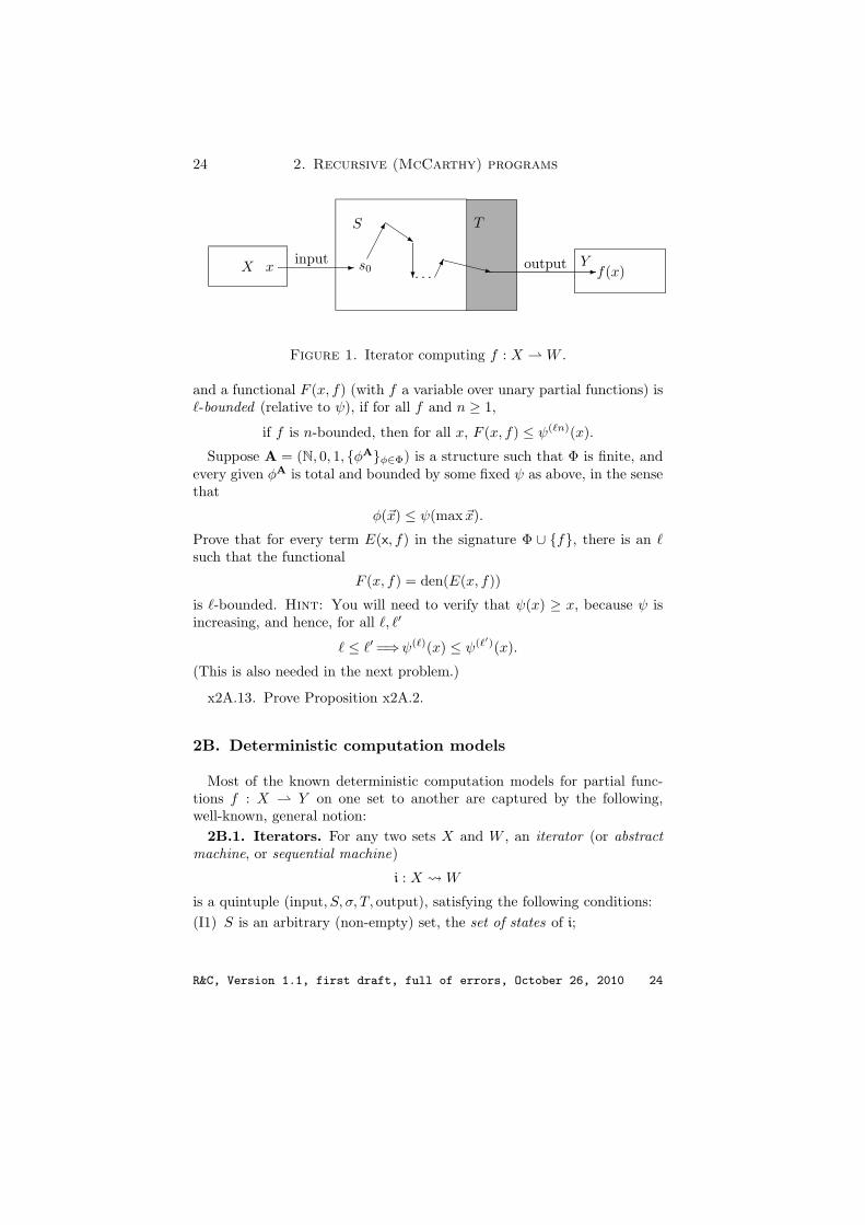
Figure 1. Iterator computing f : X ⇀ W .

and a functional F (x, f) (with f a variable over unary partial functions) isℓ-bounded (relative to ψ), if for all f and n ≥ 1,

if f is n-bounded, then for all x, F (x, f) ≤ ψ(ℓn)(x).

Suppose A = (N, 0, 1, {φA}φ∈Φ) is a structure such that Φ is finite, andevery given φA is total and bounded by some fixed ψ as above, in the sensethat

φ(~x) ≤ ψ(max ~x).

Prove that for every term E(x, f) in the signature Φ ∪ {f}, there is an ℓsuch that the functional

F (x, f) = den(E(x, f))

is ℓ-bounded. Hint: You will need to verify that ψ(x) ≥ x, because ψ isincreasing, and hence, for all ℓ, ℓ′

ℓ ≤ ℓ′ =⇒ψ(ℓ)(x) ≤ ψ(ℓ′)(x).

(This is also needed in the next problem.)

x2A.13. Prove Proposition x2A.2.

2B. Deterministic computation models

Most of the known deterministic computation models for partial func-tions f : X ⇀ Y on one set to another are captured by the following,well-known, general notion:

2B.1. Iterators. For any two sets X and W , an iterator (or abstract

machine, or sequential machine)

i : X W

is a quintuple (input, S, σ, T, output), satisfying the following conditions:

(I1) S is an arbitrary (non-empty) set, the set of states of i;


2B. Deterministic computation models 25

(I2) input : X → S is the input function of i;(I3) σ : S → S is the transition function of i;(I4) T ⊆ S is the set of terminal states of i, and s ∈ T =⇒ σ(s) = s;(I5) output : T →W is the output function of i.

An example of an iterator that we have already seen is the while pro-gram (26) associated with an arbitrary tail recursive program (25), providedthe algebra A is total: the states are all k-tuples ~u ∈ Ak, test(~u) defineswhich of them are terminal, and the input, output and transition functionsare explicit in A.

A partial computation of i is any finite sequence (s0, . . . , sn) such thatfor all i < n, si is not terminal and σ(si) = si+1, and it is convergent if,in addition, sn ∈ T . Note that (with n = 0), this includes every one-termsequence (s), and (s) is convergent if s ∈ T . We write

s→∗is′ there is a convergent computation with s0 = s, sn = s′,(29)

and we say that i computes a partial function f : X ⇀W if

f(x) = w ⇐⇒ (∃s ∈ T )[input(x) →∗is & output(s) = w].(30)

It is clear that there is at most one convergent computation starting fromany state s0, and so exactly one partial function i : X ⇀ W computed byi. The computation of i on x is the finite sequence

Compi(x) = (input(x), s1, . . . , sn, output(sn)) (x ∈ X, i(x)↓),(31)

such that (input(x), s1, . . . , sn) is a convergent computation, and its length

Timei(x) = n+ 2(32)

is the natural time complexity of i.

There is little structure to this definition of course, and the importantproperties of specific computation models derive from the judicious choiceof the set of states and the transition function, but also the input andoutput functions. The first two depend on what operations (on various datastructures) are assumed as given (primitive) and regulate how the iteratorcalls them, while the input and output functions often involve representing

the members of X and W in some specific way, taking for example numbersin unary or binary notation if X = W = N. We will not study computationmodels in these Notes, beyond the few simple facts in the remainder of thissection which relate them to recursive programs.

Fix an iterator i, let

Ai = {0, 1, } ⊎X ⊎W ⊎ Sbe the disjoint union of the indicated sets, and extend the iterator functionsinput, σ, output to all of Ai by setting their value = 0 on inappropriate



arguments. We “identify” T ⊆ Ai with its dual characteristic function

χT (s) =

{0, if s ∈ T,

1, otherwise,

and we set

Ai = ({0, 1, } ⊎X ⊎W ⊎ S, input, σ, T, output).

This is the algebra associated with i. The recursive program associated with

i has just two equations:

Ei :

{f(x) = g(input(x)),g(s) = if (s ∈ T ) then output(s) else g(σ(s)).

(33)

Lemma x2B.1. For each iterator i and the associated recursive program

E ≡ Ei on Ai and for all x ∈ X,

i(x) = fAi

(x).

In particular, the partial function computed by an iterator i : X W is

tail recursive in the associated algebra Ai.

Proof. Let f, g be the partial functions computed by the program Ei,and define g : S ⇀ W by

g(s) = w ⇐⇒ (∃s′ ∈ T )[s→∗is′ & output(s′) = w].

It is clear that g satisfies the recursive equation for g in Ei, and so

g⊑ g.

For the converse inclusion, we show by induction on n that

if [s→ s1 → · · · → sn ∈ T ], then output(sn) = g(s).

This is trivial at the base n = 0. At the induction step, the hypothesis

s→ s1 → · · · → sn+1 ∈ T

gives output(sn+1) = g(s1), by the induction hypothesis; but s1 = σ(s),and so

g(s) = g(σs) = g(s1) = output(sn+1)

as required. This establishes that g = g, and so

i(x) = g(input(x)) = g(input(x)) = f(x)

as required. ⊣



2B.2. Recursive machines. For each recursive program E of signa-ture Φ as in (17) and each Φ-algebra A, we define the recursive machine

i = i(A, E) which computes the partial function fA

E as follows.

The states of i are all finite sequences s of the form

a0 . . . am−1 : b0 . . . bn−1

where the elements a0, . . . , am1, b0, . . . , bn−1 of s satisfy the following con-

ditions:

• Each ai is a function symbol in Φ, or one of f1, . . . , fK , or a closedΦ[A]-term, or the special symbol ?, and

• each bj is an individual constant, i.e., bi ∈ A.

The special symbol ‘:’ has exactly one occurrence in each state, and the

sequences ~a,~b are allowed to be empty, so that the following sequences arestates (with x ∈M):

x : : x :

The terminal states of i are the sequences of the form

: w

i.e., those with no elements on the left of ‘:’ and just one constant on theright; and the output function of i simply reads this constant w, i.e.,

output( : w) = w.

The states, the terminal states and the output function of i depend onlyon Φ, A and the function variables which occur in E. The input functionof i depends also on the head term E0(~x) of E,

input(~x) ≡ E0(~x) :

The transition function of i is defined by the seven cases in the TransitionTable 1, i.e.,

σ(s) =

{s′, if s→ s′ is a special case of some line in Table 1,

s, otherwise,

and it is a function, because for a given s (clearly) at most one transitions→ s′ is activated by s. Notice that only the external calls depend on thealgebra A, and only the internal calls depend on the program E—and so,in particular, all programs with the same body share the same transitionfunction.

An illustration of how these machines compute is given in Figure 2.



(pass) ~a x : ~b → ~a : x ~b (x ∈ A)

(e-call) ~a φi : ~x ~b → ~a : φA

i (~x) ~b

(i-call) ~a fi : ~x ~b → ~a Ei(~x) : ~b

(comp) ~a h(F1, . . . , Fn) : ~b → ~a h F1 · · · Fn : ~b

(br) ~a if (F = 0) then G else H : ~b → ~a G H ? F : ~b

(br0) ~a G H ? : 0 ~b → ~a G : ~b

(br1) ~a G H ? : y( 6= 0) ~b → ~a H : ~b

• The underlined words are those which trigger a transition and change.• ~x = x1, . . . , xn is an n-tuple of individual constants (from A).• In the external call (e-call), φi ∈ Φ and arity(φi) = ni = n.• In the internal call (i-call), pi is an n-ary function variable of A defined

by the equation pi(~x) = Ai.• In the composition transition (comp), h is a (constant or variable)

function symbol with arity(h) = n.

Table 1. Transition Table for the recursive machine i(A, E).

Theorem x2B.2. Suppose A is a Φ-algebra, E is a Φ-program with func-

tion variables f1, . . . , fK , f1, . . . , fK are the mutual fixed points of E in A,

and M(f1, . . . , fK) is a closed sig(E)[A]-term. Then for every w ∈ A,

den(M(f1, . . . , fK) = w ⇐⇒ M(f1, . . . , fK) : →∗i(A,E) : w.(34)

In particular, with M ≡ E0(~x)

denA(E,~x) = w ⇐⇒ E0(~x) →∗i(A,E) : w,

and so the iterator i(A, E) computes den(M).

Outline of proof. First we define the partial functions computed byi(A, E) in the indicated way,

fi(~xi) = w ⇐⇒ fi(~xi) : →∗ : w,



f(2, 3) : (comp)

f 2 3 : (pass, pass)

f : 2 3 (i-call)

if (2 = 0) then 3 else S(f(Pd(2), 3)) : (br)

3 S(f(Pd(2), 3)) ? 2 : (pass)

3 S(f(Pd(2), 3)) ? : 2 (br2)

S(f(Pd(2), 3)) : (comp)

S f(Pd(2), 3) : (comp)

S f Pd(2) 3 : (pass)

S f Pd(2) : 3 (comp)

S f Pd 2 : 3 (pass)

S f Pd : 2 3 (e-call)

S f : 1 3 (i-call)

S if (1 = 0) then 3 else S(f(Pd(1), 3)) : (br), (comp many times)

S S f Pd(1) 3 : (pass)

S S f Pd(1) : 3 (comp)

S S f Pd 1 : 3 (pass)

S S f Pd : 1 3 (e-call)

S S f : 0 3 (i-call)

S S if (0 = 0) then 3 else S(f(Pd(0), 3)) : (br), (comp many times), (pass)

S S 3 S f(Pd(0), 3) ? : 0 (br0)

S S 3 : (pass)

S S : 3 (e-call)

S : 4 (e-call)

: 5

Figure 2. The computation of 2 + 3 by the programf(i, x) = if (i = 0) then x else S(f(Pd(i), x)).

and show by an easy induction on the term F the version of (34) for these,

denA(F (f1, . . . , fK)) = w ⇐⇒ F : →∗i(A,E) : w.(35)

When we apply this to the terms Ei{~xi :≡ ~xi} and use the form of theinternal call transition rule, we get

denA(Ei(~xi, f1, . . . , fK)) = w ⇐⇒ fi(~xi) = w,



which means that the partial functions f0, . . . , fK satisfy the system (20),

and so f0 ≤ f0, . . . , fK ≤ fK .Next we show that for any closed term F as above and any system

f0, . . . , fK of solutions of (20),

F : →∗ w=⇒ denA(F (f1, . . . , fK)) = w.

This is done by induction of the length of the computation which establishesthe hypothesis, and setting F ≡ E0{~xi :≡ ~xi}, it implies that

f0 ≤ f0, . . . , fK ≤ fK .

It follows that f0, . . . , fK are the least solutions of (20), i.e., fi = f i, whichtogether with (35) completes the proof.

Both arguments appeal repeatedly to Problem x2B.5, which is simplebut basic. ⊣

There are two obvious complexity measures of the recursive machinei(A, E) associated with A and E,

Timei(~x) = the length of the computation starting with E0(~x) :(36)

Timeei(~x) = the number of external calls in this computation.(37)

We will compare them in the next chapter with the natural, “structural”complexity measures which can be defined directly for each recursive pro-gram E, without reference to its implementations.

2B.3. Simulating Turing machines with Nb-programs. To con-nect these complexity measures with classical, Turing-machine time com-plexity, we show here (in outline) one typical result:8

Proposition x2B.3. If a function f : N → N is computable by a Turing

machine M in time T (log n) for n > 0, then there is a natural number kand an Nb-program E which computes f with Timei(n) ≤ kT (log n) for

n > 0, where i = i(Nb, E) is the recursive machine associated with E.

We are assuming here that the input n is entered on a tape of M inbinary notation (which is why we express the complexity as a function oflog n), but other than that, the result holds in full generality: the machineM may or may not have separate input and output tapes, it may have oneor many, semi-infinite or infinite work tapes, etc. An analogous result holdsalso for functions of several variables.

Outline of proof. Consider the simplest case, where M has a two-way infinite tape and only one symbol in its alphabet, 1. We use 0 todenote the blank symbol, so that the “full configuration” of a machine at astage in a computation is a triple (q, τ, i), where q is a state, τ : Z → {0, 1},

8This is not needed for the sequel, and its proof assumes some familiarity with Turingmachines.



τ (j) = 0 for all but finitely many j’s, and i ∈ Z is the location of thescanned cell. If we write τ as a pair of sequences emanating from thescanned cell y0

· · ·x3x2x1x0y0↑

y1y2y3 · · ·

one “growing” to the left and the other to the right, we can then code (τ, i)by the pair of numbers

(x, y) = (∑

j xj2j ,

∑j yj2

j).

Notice that y0 = parity(y) and x0 = parity(x), so that the scanned symboland the symbol immediately to its left are computed from x and y by Nb-operations. The input configuration for the number z is coded by the triple(q0, 0, z), with q0 the starting state, and all machine operations correspondto simple Nb-functions on these codes. For example:

move to the right : x 7→ 2x+ parity(y), y 7→ iq2(y),

move to the left : x 7→ iq2(x), y 7→ 2y + parity(x),

where (in the notation of (10)),

2x+ parity(y) = if (parity(y) = 0) then em2(x) else om2(x).

It is not difficult to write a Nb-program using these functions which simu-lates M .

We leave for the problems the details and the proof of the general result.⊣

Problems for Section 2B

x2B.4. For the following three recursive programs in Nu:

f(x) = S(f(x))(E1)

f(x) = f(g(x))(E2)

g(x) = x,

f(x, y) = f1(f(x, y), y).(E3)

f1(x, y) = x,

(1) Which partial functions satisfy them?(2) Which partial functions do they compute, and in what way do their

computations differ?



x2B.5 (Transition locality). Prove that if s0, s1, . . . , sn is a partial com-

putation of i(A, E) and ~a∗,~b∗ are such that the sequence ~a∗s0~b∗ is a state,

then the sequence

~a∗s0~b∗,~a∗s1~b

∗, . . . ,~a∗sn~b∗

is also a partial computation of i(A, E).

x2B.6. Fill in the details in the proof of Theorem x2B.2.

x2B.7 (Stack discipline). (1) Show that for every program E in a total

algebra A, and every closed sig(E)[A]-term M , there is no computation ofi(A, E) of the form

M : → s1 → · · · → sm(38)

which is stuck, i.e., the state sm is not terminal and there is no s′ such thats→ s′.

(2) Show that if A is a partial algebra, M is a closed sig(E)[A]-term andthe finite computation (38) is stuck, then its last state sm is of the form

~a φj : y1, . . . , ynj~b

where φj is a primitive function of A of arity nj and φj(y1, . . . , ynj) ↑.

x2B.8. Give a detailed proof of Proposition x2B.3 for a Turing machineM which has two, two-way tapes, K symbols in its alphabet and computesa partial function f : N2 ⇀ N of two arguments. Hint: If there are twosymbols a and b, represent the blank by 00, a by 01 and b by 10.

Symbolic computation. The symbolic recursive machine i = is(Φ, E)associated with a signature Φ and a Φ-program E is defined as follows.

The states of i are all finite sequences s of the form

a0 . . . am−1 : b0 . . . bn−1

where the elements a0, . . . , am1, b0, . . . , bn−1 of s satisfy the following con-

ditions:

• Each ai is a function symbol in Φ or or one of f1, . . . , fK , or a pure,algebraic sig(E)-term, or the special symbol ?, and

• each bj is a pure, algebraic Φ-term.

The transitions of i are those listed for a recursive machine in Table 1,except for the following three which are modified as follows:

(e-call) ~a φi : ~x ~b → ~a : φi(~x) ~b

(br0) ~a G H ? : b0 ~b → ~a G : ~b (if b0 = 0)

(br1) ~a G H ? : b0 ~b → ~a H : ~b (if b0 6= 0)



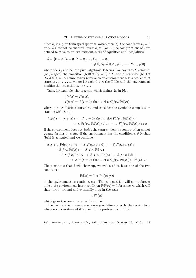
Since b0 is a pure term (perhaps with variables in it), the conditions b0 = 0or b0 6= 0 cannot be checked, unless b0 is 0 or 1. The computations of i aredefined relative to an environment, a set of equalities and inequalities

E = {0 = 0, P0 = 0, P1 = 0, . . . , Pm−1 = 0,

1 6= 0, N0 6= 0, N1 6= 0, . . . , Nn−1 6= 0},where the Pi and Nj are pure, algebraic Φ-terms. We say that E activates

(or justifies) the transition (br0) if (b0 = 0) ∈ E , and E activates (br1) if(b0 6= 0) ∈ E . A computation relative to an environment E is a sequence ofstates s0, s1, . . . , sn where for each i < n the Table and the environmentjustifies the transition si → si+1.

Take, for example, the program which defines 2x in Nu,

fE(u) = f(u, u),

f(u, v) = if (v = 0) then u else S(f(u,Pd(v))

where u, v are distinct variables, and consider the symbolic computationstarting with fE(u) :

fE(u) : → f(u, u) : → if (u = 0) then u else S(f(u,Pd(u))) :

→ u S(f(u,Pd(u))) ? u : → u S(f(u,Pd(u))) ? : u

If the environment does not decide the term u, then the computation cannotgo any further, it stalls. If the environment has the condition u 6= 0, then(br1) is activated and we continue:

u S(f(u,Pd(u)) ? : u → S(f(u,Pd(u))) : → S f(u,Pd(u)) :

→ S f u,Pd(u) : → S f u,Pd u :

→ S f u,Pd : u → S f u : Pd(u) → S f : u Pd(u)

→ S if (u = 0) then u else S(f(u,Pd(u))) : Pd(u) . . .

The next time that ? will show up, we will need to have one of the twoconditions

Pd(u) = 0 or Pd(u) 6= 0

in the environment to continue, etc. The computation will go on foreverunless the environment has a condition Pdn(u) = 0 for some n, which willthen turn it around and eventually stop in the state

: Sn(u)

which gives the correct answer for u = n.The next problem is very easy, once you define correctly the terminology

which occurs in it—and it is part of the problem to do this.



x2B.9. Fix a Φ-algebra and a Φ-program E, and suppose that

M(x1, . . . , xn) : → s1 → · · · → : M

is a computation of the recursive machine of E which computes the valueof the closed sig(E)[A] term M(x1, . . . , xn) with the indicated parameters.Prove that there is an environment E in the distinct variables v1, . . . , vn

which is sound for x1, . . . , xn in A, such that the given computation canbe obtained from the symbolic computation relative to E and starting withM(v1, . . . , vn) by replacing each vi in it by xi.

x2B.10. Prove that Pd(x) is not (N, 0, 1, S)-recursive.

There are many other applications of symbolic computation, but we willnot cover the topic. (And it is rather surprising that the simple and basicProblem x2B.10 seems to need it. Perhaps there is a simpler proof.)

2C. Finite non-determinism

Much of the material in Section 2B can be extended easily to non-de-

terministic computation models, in which the transition function σ : S → Sis replaced by a relation σ ⊆ S × S, usually assumed total, i.e., such that(∀s)(∃s′)σ(s, s′). We do not have much use for these here, and the modeltheory of the algebras associated with them is a bit messy. We will coveronly the most useful, special case of finite non-determinism.

For any two sets X,Y , a finitely non-deterministic iterator i : X Y isa tuple

i = (input, S, σ1, . . . , σK , T, output)

which satisfies (I1) – (I5) in Section 2B.1 except that (I3) is replaced bythe obvious

(I3′) for every i = 1, . . . ,K, σi : S → S.

So i has K transition functions. Computations are defined as before, exceptthat we allow transitions si+1 = σj(si) by any one of the transition func-tions, so that, for example, s, σ1(s), σ3(σ(s)), . . . is a partial computation.This presents the possibility that the machine may produce more than onevalue on some input, and we must be careful in defining what if means fori to compute some f : X ⇀ Y .

A non-deterministic iterator i computes f : X ⇀ Y on S ⊆ X if

f(x) = y ⇐⇒ (∃s ∈ T )[input(x) →∗is & output(s) = w] (x ∈ S).(39)

In other words, i : X Y computes f on S ⊆ X if and only if when-

ever f(x)↓ with x ∈ X, then at least one convergent computation starting


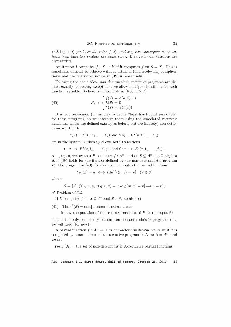
2C. Finite non-determinism 35

with input(x) produces the value f(x), and any two convergent computa-

tions from input(x) produce the same value. Divergent computations aredisregarded.

An iterator i computes f : X ⇀ Y if it computes f on S = X. This issometimes difficult to achieve without artificial (and irrelevant) complica-tions, and the relativized notion in (39) is more useful.

Following the same idea, non-deterministic recursive programs are de-fined exactly as before, except that we allow multiple definitions for eachfunction variable. So here is an example in (N, 0, 1, S, φ):

E∗ :

f(~x) = φ(h(~x), ~x)h(~x) = 0h(~x) = S(h(~x)).

(40)

It is not convenient (or simple) to define “least-fixed-point semantics”for these programs, so we interpret them using the associated recursivemachines. These are defined exactly as before, but are (finitely) non-deter-ministic: if both

f(~u) = E1(~u, f1, . . . , fn) and f(~u) = E2(~u, f1, . . . , fn)

are in the system E, then iE allows both transitions

f : ~x → E1(~x, f1, . . . , fn) : and f : ~x → E2(~x, f1, . . . , fn) :

And, again, we say that E computes f : An ⇀ A on S ⊆ An in a Φ-algebraA if (39) holds for the iterator defined by the non-deterministic programE. The program in (40), for example, computes the partial function

fE∗(~x) = w ⇐⇒ (∃n)[g(n, ~x) = w] (~x ∈ S)

where

S = {~x | (∀n,m, u, v)[g(n, ~x) = u & g(m,~x) = v] =⇒u = v},cf. Problem x2C.5.

If E computes f on S ⊆ An and ~x ∈ S, we also set

(41) TimeE(~x) = min{number of external calls

in any computation of the recursive machine of E on the input ~x}This is the only complexity measure on non-deterministic programs thatwe will need (for now).

A partial function f : An ⇀ A is non-deterministically recursive if it iscomputed by a non-deterministic recursive program in A for S = An, andwe set

recnd(A) = the set of non-deterministic A-recursive partial functions.



The distinction between deterministic and non-deterministic algorithmsunderlies some of the most interesting and deep problems of computationtheory, including the central P=NP? problem. Closer to the questionswe have been considering, the results of Stolboushkin and Taitslin [1983]and Tiuryn [1989] that we mentioned above were established to distinguishdeterministic from non-deterministic tail-recursion (in the terminology wehave been using) as well as (deterministic) tail recursion from full recur-sion. We will not go into the topic in this Version, except for the followingdiscussion of a non-deterministic algorithm for the gcd (and coprimeness)which is relevant to the proof of Theorem A in the Introduction that wewill give in Chapter 6.9

Theorem x2C.1 (Pratt’s nuclid algorithm). Consider the following non-

deterministic recursive program EP in the algebra Nε = (N, 0, 1,%) of the

Euclidean:

fP (a, b) = nuclid(a, b, a, b)

nuclid(a, b,m, n) = if (n 6= 0) then nuclid(a, b, n, choose(a, b,m)%n)

else if (a%m 6= 0) then nuclid(a, b,m, a%m)

else if (b%m 6= 0) then nuclid(a, b,m, b%m)

else m

choose(a, b,m) = a, choose(a, b,m) = b, choose(a, b,m) = m.

If a ≥ b ≥ 1, then fP (a, b) = gcd(a, b).

Proof. Fix a ≥ b ≥ 1, and let

(m,n) → (m′, n′) ⇐⇒(n 6= 0 & m′ = n

& [n′ = m%n ∨ n′ = a%n ∨ n′ = b%n])

∨(n = 0 & a%m 6= 0 & m′ = m & n′ = a%m

)

∨(n = 0 & b%m 6= 0 & m′ = m & n′ = b%m

).

This is the non-deterministic transition function of the main loop of theprogram (with a, b omitted), and it has the obvious property that it respectsthe property m > 0. The terminal states are

T (a, b,m, n) ⇐⇒ n = 0 & m | a & m | b,and the output on a terminal (a, b,m, 0) is m.

It is obvious that there is at least one computation which outputs gcd(a, b),because one of the choices at each step is the one that the Euclidean would

9This theorem and Problems x2C.6 – x2C.9 are unpublished results of Vaughan Prattand are presented here with his permission.


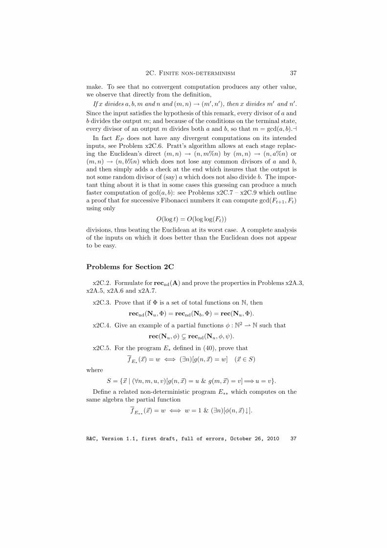
2C. Finite non-determinism 37

make. To see that no convergent computation produces any other value,we observe that directly from the definition,

If x divides a, b,m and n and (m,n) → (m′, n′), then x divides m′ and n′.

Since the input satisfies the hypothesis of this remark, every divisor of a andb divides the output m; and because of the conditions on the terminal state,every divisor of an output m divides both a and b, so that m = gcd(a, b).⊣

In fact EP does not have any divergent computations on its intendedinputs, see Problem x2C.6. Pratt’s algorithm allows at each stage replac-ing the Euclidean’s direct (m,n) → (n,m%n) by (m,n) → (n, a%n) or(m,n) → (n, b%n) which does not lose any common divisors of a and b,and then simply adds a check at the end which insures that the output isnot some random divisor of (say) a which does not also divide b. The impor-tant thing about it is that in some cases this guessing can produce a muchfaster computation of gcd(a, b): see Problems x2C.7 – x2C.9 which outlinea proof that for successive Fibonacci numbers it can compute gcd(Ft+1, Ft)using only

O(log t) = O(log log(Ft))

divisions, thus beating the Euclidean at its worst case. A complete analysisof the inputs on which it does better than the Euclidean does not appearto be easy.

Problems for Section 2C

x2C.2. Formulate for recnd(A) and prove the properties in Problems x2A.3,x2A.5, x2A.6 and x2A.7.

x2C.3. Prove that if Φ is a set of total functions on N, then

recnd(Nu,Φ) = recnd(Nb,Φ) = rec(Nu,Φ).

x2C.4. Give an example of a partial functions φ : N2 ⇀ N such that

rec(Nu, φ) ( recnd(Nu, φ, ψ).

x2C.5. For the program E∗ defined in (40), prove that

fE∗(~x) = w ⇐⇒ (∃n)[g(n, ~x) = w] (~x ∈ S)

where

S = {~x | (∀n,m, u, v)[g(n, ~x) = u & g(m,~x) = v] =⇒u = v}.Define a related non-deterministic program E∗∗ which computes on the

same algebra the partial function

fE∗∗(~x) = w ⇐⇒ w = 1 & (∃n)[φ(n, ~x)↓ ].



The remaining problems in this section are due to Vaughan Pratt.

x2C.6. Prove that the program EP has no divergent (infinite) computa-tions on inputs (a, b, a, b) with a ≥ b ≥ 1. Hint: Show convergence of themain loop under the hypothesis by induction on max(m,n) and within thisby induction on n.

The complexity estimate for Pratt’s algorithm depends on some classicalidentities that relate the Fibonacci numbers.

x2C.7. Prove that for all t ≥ 1 and m ≥ t,

Fm(Ft+1 + Ft−1) = Fm+t + (−1)tFm−t.(42)

Hint: Show in sequence, by direct computation, that

ϕϕ = −1; ϕ+1

ϕ=

√5; ϕ+

1

ϕ= −

√5; Ft+1 + Ft−1 = ϕt + ϕt.

x2C.8. (1) Prove that for all odd t ≥ 2 and m ≥ t,

Fm+t%Fm = Fm−t (t odd).(43)

(2) Prove that for all even t ≥ 2 and m ≥ t,

Fm+t%Fm = Fm − Fm−t,(44)

Fm%(Fm+t%Fm) = Fm−t,(45)

Hint: For (2), check that for t ≥ 2, 2Fm−t < Fm.

x2C.9. Fix t ≥ 2. Prove that for every s ≥ 1 and every u such thatu ≤ 2s and t − u ≥ 2, there is a computation of Pratt’s algorithm whichstarts from (Ft+1, Ft, Ft+1, Ft) and reaches a state (Ft+1, Ft, ?, Ft−u) doingno more than 2s divisions.

Infer that for all t ≥ 3,

TimeEP (Ft+1, Ft) ≤ 2⌈log(t− 2)⌉ + 1 = O(log(t− 1)).(46)


recursive (mccarthy) programs - uclaynm/rc/chap2.pdfchapter 2 recursive (mccarthy) programs...

Documents