Recursive Thick Modeling and the Choice of Monetary Policy in Mexico

(Preliminary and Incomplete: May 2006)

Arnulfo Rodriguez*

Pedro N. Rodriguez∗∗

* Dirección General de Investigación Económica, Banco de México. I thank Alberto Torres, Jéssica Roldán and Julio Pierre-Audain for familiarizing me with analytical and computational tools of key importance to this research work. I also thank Pedro León de la Barra and Mario Oliva for excellent research assistance. The opinions in this paper correspond to the authors and do not necessarily reflect the point of view of Banco de México. ∗∗ Departamento de Estadística e Investigación Operativa II, Universidad Complutense de Madrid.

2

Recursive Thick Modeling and the Choice of Monetary Policy in Mexico

(Preliminary and Incomplete: May 2006)

Arnulfo Rodriguez

Pedro N. Rodriguez

Abstract. By following the spirit in Favero and Milani (2005), we use recursive thick modeling to take into account model uncertainty for the choice of optimal monetary policy. We consider an open economy model and generate multiple models for only the aggregate demand and aggregate supply. We use a rolling window of fixed size for the estimations. The Schwarz´s Bayesian Information Criterion (BIC) and the adjusted R2 are the two statistical criteria selection methods used to rank all of the generated output gap and core inflation models. Models are constructed by matching the rankings of aggregate demand and aggregate supply and adding other specifications for the rest of the variables. The weights are based on BIC and 2R in sample criteria. The main results show that recursive thick modeling with equal weights approximates the recent historical behavior of nominal interest rates in Mexico better than a weighted average based on any criterion. Furthermore, recursive thick modeling with simple and weighted averages works better than recursive thin modeling.

JEL Classification: C61, E61 Keywords: macroeconomic policy, model uncertainty, optimal control, monetary policy, inflation targeting.

3

INTRODUCTION

An approach for dealing with parameter instability and non-linearity is proposed by Pesaran

and Timmermann (1995) in the context of small models. They address those potential

problems by using recursive modeling. Favero and Milani (2005) not only do they use the

same approach in the analysis of optimal monetary policy for the US economy, but they

also complement it with the thick modeling approach proposed by Granger and Jeon (2004).

Favero and Milani (2005) generate 2k models in every period by making all of the possible

combinations from a set of k regressors. This way of combining regressors allows them to

take into account the uncertainty in the number of lags with which the relevant variables

enter into both the aggregate demand and aggregate supply specifications. Here we also do

the same to the analysis of optimal monetary policy in Mexico in order to assess the

relevance of model uncertainty.

Unlike Favero and Milani (2005), we consider an open economy model. The 2k

models are only generated for the output gap and core inflation. We use a rolling window

of fixed size for the estimations. The Schwarz´s Bayesian Information Criterion (BIC) and

the adjusted R2 are the two statistical criteria selection methods used to rank all of the

generated output gap and core inflation models. However, the results show that the

rankings given by one criterion do not necessarily correspond to the rankings obtained from

the other. The output gap and core inflation models are grouped together according to their

ranking – i.e. the best output gap model with the best core inflation model, the second best

output gap model with the second best core inflation model, etc. We obtain the optimal

policies derived from all of the relevant models.1

The lack of correspondence between the rankings given by the statistical criteria

makes the decision to exclusively rely on the best model in every period somewhat

difficult. By considering the rest of the models we take into account model uncertainty for

1 Models in which monetary policy does not play a role in controlling core inflation through the demand channel are not considered.

4

determining optimal monetary policy. It is worth mentioning that the resulting thick line

reflects the degree of model uncertainty derived only from the dynamic structure of the

economy – i.e. which relevant lags to consider for some variables. Other types of

uncertainty as defined by Jenkins and Longworth (2002) and related to additive shocks,

duration of shocks and data are not addressed in this paper. Neither do we directly

incorporate parameter uncertainty à la Brainard (1967) to determine its effect on optimal

policy. Söderström (2002) studies the effect of uncertainty in the inflation persistence

parameter on optimal policy. The other approach to deal with model uncertainty is robust

control as in Hansen and Sargent (2003) and Onatski and Stock (2002).

The implied optimal nominal interest rates for any given period substantially vary

across specifications. Moreover, we are able to do a better tracking job of the actual

nominal interest rates when we obtain the simple and weighted averages for the optimal

nominal interest rates. These results argue in favor of making it necessary to take model

uncertainty into account when setting monetary policy.

By statistically comparing the MSEs obtained from the average optimal policies

given by different preference parameters, we are able to reveal only a range in which the

revealed preference parameters could be.2 We do the same statistical comparison between

simple and weighted averages only for the preference parameters 3.0,5.0 == φα . We find

that simple averages work better than weighted averages. The results also show both

reductions in bias and standard deviation in tracking the actual nominal interest rates when

using either simple or weighted averages of optimal nominal interest rates.

The results also indicate that the set of variables belonging to the best specification

for both the output gap and core inflation is changing through time.

In this paper we take the uncertainty analysis done by Favero and Milani (2005).

Our basic model is a modified version of the dynamic aggregate supply-aggregate demand

2 We cannot exactly reveal the true preference parameters since our analysis only considers six cases. A finer grid search would get us very close to the true preference parameters. See Roldán-Peña (2005) for revealing preference parameters with finer grids.

5

framework used by Rudebusch and Svensson (1999). The original framework was modified

to include open economy variables. The dynamic homogeneity condition is imposed on the

Phillips curve for core inflation, which is similar to the one used by Contreras and García

(2002).3 The IS curve is similar to the one used by Ball (1999). The equations used are:

πεββπβπ ttt

ct

ct eudex +−++= −− inf)1( 12211 (1)

xttt

usttt rltcrxxx εγγγγγ +++++= −−− 14312110 (2)

Equation (1) is an open economy Phillips curve where core inflation c

tπ is affected by its

own lag ct 1−π , the output gap second lag 2−tx , and the sum of the contemporaneous nominal

exchange rate percentage depreciation and the external inflation teude inf . We impose the

dynamic homogeneity condition in equation (1) to guarantee long run inflation neutrality on

output.4

Equation (2) is an open economy IS equation where the output gap tx is affected by

its own lag 1−tx , the lag of the US output gap ustx 1− , the lag of the ex-post real interest rate

1−tr and the contemporaneous value of the natural log of the real exchange rate tltcr . πε t

and xtε are the respective white noise shocks. We use monthly data for core inflation,

output gap, the real exchange rate and the ex-post real interest rate.

Under the restrictions given by equations 1-2 along with other specifications for

exogenous variables, the central bank minimizes an intertemporal loss function by

optimally setting the nominal interest rate. Initially, it is assumed that this single model

3 As opposed to the Phillips curve used by those authors, ours does not have a forward-looking inflation component. The reasons for not having included forward-looking variables will be given in the next sections. 4 Data was obtained from Banco de México. The output gaps are percentage deviations of the seasonal adjusted Index of General Economic Activity (IGAE) and the seasonal adjusted US Industrial Production Index from their respective output potential. The output potentials represent an average of a linear trend and a Hodrick-Prescott filter. The log of the real exchange rate is the natural logarithm of the US-Mexico real exchange rate index (1997 = 1.0). The monthly nominal interest rate was obtained from the 28-day Mexican government T-bill (CETES).

6

contains the correct representation of the economy and that the model parameters are

constant over time.

PARAMETER INSTABILITY

Using monthly data over the period 1996:09-2004:06, the estimated equations are as

follows5:

πεππ ttt

ct

ct eudex ++−= −− inf019446.0001480.0980553.0 21 (3)

(0.0000) (0.8593)

Xttt

usttt rltcrxxx ε+−+++= −−− 111 036376.0042619.0336692.0528036.0221060.0 (4)

(0.1773) (0.0000) (0.0000) (0.9552) (0.0385) To evaluate the potential parameter instability we re-estimate each equation by considering

two different sub-samples. For the core inflation equation, the sub-samples estimation

yields:

1996:10 – 1999:05 πεππ ttt

ct

ct eudex ++−= −− inf049148.0002188.0950851.0 21 (5)

(0.0000) (0.9394) 1999:06 – 2004:06 πεππ ttt

ct

ct eudex +−−= −− inf008710.0006685.0008711.1 21 (6)

(0.0000) (0.2092) For the output gap equation, the sub-samples estimation yields: 1996:09 – 1999:12 X

tttusttt rltcrxxx ε+−−++= −−− 111 030888.0893024.2069202.0588008.0301036.0 (7)

(0.1675) (0.0001) (0.5394) (0.1731) (0.2263) 2000:01 – 2004:06 X

tttusttt rltcrxxx ε++−++−= −−− 111 007044.0185126.4620912.0115780.0752512.0 (8)

(0.0355) (0.3548) (0.0000) (0.0150) (0.7830)

5 Values in parenthesis are p-values.

7

We take these results as an indication of parameter instability of economic

relevance. Performing a Chow test of the null of parameter stability on the output gap

equation, we find a potential breakpoint at date 2000:01 and reject the hypothesis of no

breakpoint at the 5% significance level. Doing the same for the core inflation equation we

find a potential breakpoint at date 1999:06. However, since the variances of the residuals

for each of the sub-samples are significantly different, a Chow test is no longer satisfactory,

so we perform a Wald test, as suggested by Watt (1979) and Honda (1982), which provides

conclusive evidence against the stability of core inflation: we reject the hypothesis of equal

parameters at the 5% significance level.

Favero and Milani (2005) explain that recursive modeling consists of updating the

economic model by choosing the best possible representation of the unknown Data

Generating Process over a base set of k regressors. They also take into account the models

not chosen in order to consider specification uncertainty.

Estimations are obtained by using a rolling window of fixed length and take into

account the dynamic homogeneity property as well as some parameters restrictions which

reflect some assumptions about long-term values for the real interest rate and the real

exchange rate. The window size does not come from an optimization procedure and is set

equal to fifty two observations. We use monthly data from September 1996 to May 2004.

The first period estimations are obtained with data from September 1996 to December

2000. When using the rolling window of fixed length, we obtain all the optimal nominal

interest rates implied by each model for the forty two periods starting in January 2001 and

ending in June 2004. These implied optimal nominal interest rates represent one-step ahead

forecasts since we are mimicking a policy maker who optimizes a loss function subject to

specifications estimated with all the available data up to that point.

We assume no uncertainty for the real exchange rate equation and the rest of the

equations for the exogenous variables. The technical complications of allowing a forward-

looking component in the real exchange rate equation makes it very difficult to consider

8

uncertainty on this particular specification.6 In other words, estimating models derived from

all the possible combinations of k regressors could be unwieldy when using GMM for

specifications with forward-looking variables.

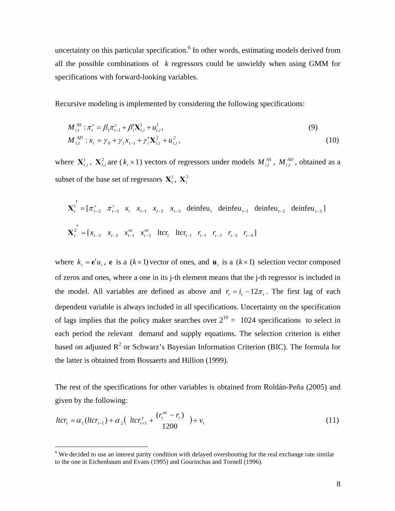
Recursive modeling is implemented by considering the following specifications:

,: 1

,1,11, ititi

ct

ct

ASti uM +′+= − Xβπβπ (9)

,: 2,

2,110, itititt

ADti uxxM +′++= − Xγγγ (10)

where 1

,itX , 2,itX are ( 1×ik ) vectors of regressors under models AS

tiM , , ADtiM , , obtained as a

subset of the base set of regressors 1tX , 2

tX

ctt 2

1 [ −=′

πX ct 3−π tx 1−tx 2−tx 3−tx tdeinfeu 1deinfeu −t 2deinfeu −t 3deinfeu −t ]

22 [ −=′

tt xX 3−tx ustx 1− us

tx 2− tltcr 1ltcr −t 1−tr 2−tr 3−tr 4−tr ]

where ii uk e′= , e is a )1( ×k vector of ones, and iu is a )1( ×k selection vector composed

of zeros and ones, where a one in its j-th element means that the j-th regressor is included in

the model. All variables are defined as above and ttt ir π12−= . The first lag of each

dependent variable is always included in all specifications. Uncertainty on the specification

of lags implies that the policy maker searches over 210 = 1024 specifications to select in

each period the relevant demand and supply equations. The selection criterion is either

based on adjusted R2 or Schwarz’s Bayesian Information Criterion (BIC). The formula for

the latter is obtained from Bossaerts and Hillion (1999).

The rest of the specifications for other variables is obtained from Roldán-Peña (2005) and

given by the following:

( ) tt

uste

ttt vrr

ltcrltcrltcr +−

++= +− 1200)(

)( 1211 αα (11)

6 We decided to use an interest parity condition with delayed overshooting for the real exchange rate similar to the one in Eichenbaum and Evans (1995) and Gourinchas and Tornell (1996).

9

tnct

nct wdd ++= −110 ππ (12)

nct

ctt πλλππ )1( −+= (13)

ust t t tde dtcrπ π+ = +

and the VAR(2) system for the exogenous external variables::

tust

ust

ust

ust

ust

ust

ust iaiaxaxaaaa ϑπππ +++++++= −−−−−− 2615241322110 (14)

tust

ust

ust

ust

ust

ust

ust sibibxbxbbbbx +++++++= −−−−−− 2615241322110 ππ (15)

tust

ust

ust

ust

ust

ust

ust zicicxcxcccci +++++++= −−−−−− 2615241322110 ππ (16)

Equations 11-13 represent the dynamic specifications for the real exchange rate, non-core

monthly inflation, monthly headline inflation as a weighted sum of its core and non-core

components and the purchasing power parity condition, respectively. The VAR(2) system

represents the dynamics for the US monthly headline inflation, US output gap and US

nominal interest rates obtained from the 3 month T-bill. See Roldán-Peña (2005) for

estimation of equations 11-16.

We take into consideration only 960 models from all the possible combinations of 10

regressors for both the aggregate supply and aggregate demand equations. This is the case

since the 26 models resulting from not having the variables rt-1, rt-2, rt-3 and rt-4 are discarded

as possible specifications for the output gap. Similarly, the 26 models resulting from not

having the variables xt, xt-1, xt-2 and xt-3 are eliminated from the set of possible

specifications for core inflation. This is done in order to take into account only models that

make monetary policy relevant to control inflation.

Finally, we combine the output gap and core inflation specifications according to

their rankings given by either BIC or adjusted R2 – i.e. the best output gap specification

with the best core inflation specification, the second best output gap specification with the

second best core inflation specification, etc. Even though the uncertainty considered here

relates only to the dynamic structure of the economy (thus omitting other factors that may

influence uncertainty), the advantage of this approach is that it allows us to account for the

number of lags with which monetary policy affects the economy.

10

Having estimated all possible models, a statistical criterion is used to select a single

model to design optimal policy for each period (recursive thin modeling). Alternatively, the

information from the whole set of models can be used in each period (recursive thick

modeling).

Thin modeling discards all but one model for each dependent variable, leaving out

of the decision-making process the information from (2k -1)*2 models – i.e. since the

uncertainty about the number of lags only applies to the aggregate demand and aggregate

supply specifications. Although the chosen model is the best according to some criterion,

exclusively relying on it means that the policy maker does not consider the uncertainty

stemming from both unstable parameters and model specification.

One problem about thin modeling pointed out by Favero and Milani (2005) has to

do with the lack of match between the ranking of models obtained from different statistical

criteria. Figures 1 and 2 show scatter plots of models ranking according to adjusted R2 and

BIC criteria for all the 960 specifications of aggregate supply and aggregate demand,

respectively.

11

Figure 1. Scatter plot of models ranking under BIC and adjusted R2 for all the 960 possible specifications of

core inflation for the last period.

12

Figure 2. Scatter plot of models ranking under BIC and adjusted R2 for all the 960 possible specifications of

the output gap for the last period.

As it can be seen from those figures, the lack of match between the ranking of

models also arises. For instance, the best output gap model according to adjusted R2 (BIC)

is ranked in the 17th (162th) place by the BIC (adjusted R2) criterion. As for the core

inflation, the best model according to adjusted R2 coincides with the best one ranked by the

BIC criterion. However, any given selection criterion is prone to producing small,

statistically insignificant differences among the best models. Dell’Aquila and Ronchetti

13

(2004) find out that ranking is unreliable in the sense that the set of undistinguishable

models can be large.

Consequently, deciding which model to choose becomes hard. One way to evaluate

the importance of this choice consists of finding how robust the key parameters are across

both time and the 960 specifications. Figures 3,4 and 5 show the variation of the long run

coefficients for the real interest rate, the US output gap and the imported inflation across

both time and specifications.7 The dotted yellow line and the solid blue line placed on the

red area indicate the average of the long-run coefficients across the 960 models and the

long-run coefficient given by the best model, respectively.

0 200 400 600 800 1000-0.08

-0.06

-0.04

-0.02

0

0.02

0.04Real interest rate effect on x in June 2004 (adjusted R-squared)

Models(ranking in descending order)

Coe

ffici

ent

0 200 400 600 800 1000-0.08

-0.06

-0.04

-0.02

0

0.02

0.04Real interest rate effect on x June 2004 (BIC)

Models(ranking in descending order)

Coe

ffici

ent

0 10 20 30 40 50-0.15

-0.1

-0.05

0

0.05Real interest rate effect on x (adjusted R-squared)

January 2001-June 2004

Coe

ffici

ent

0 10 20 30 40 50-0.15

-0.1

-0.05

0

0.05Real interest rate effect on x (BIC)

January 2001-June 2004

Coe

ffici

ent

Figure 3. Variation of the real interest rate coefficient across specifications and time.

7 Long run coefficients are obtained by adding all the coefficients of the corresponding variable for each specification.

14

0 200 400 600 800 10000

0.1

0.2

0.3

0.4

0.5

0.6

0.7US output gap effect on x in June 2004 (adjusted R-squared)

Models(ranking in descending order)

Coe

ffici

ent

0 200 400 600 800 10000

0.1

0.2

0.3

0.4

0.5

0.6

0.7US output gap effect on x in June 2004 (BIC)

Models(ranking in descending order)

Coe

ffici

ent

0 10 20 30 40 500

0.1

0.2

0.3

0.4

0.5

0.6

0.7US output gap effect on x (adjusted R-squared)

January 2001-June 2004

Coe

ffici

ent

0 10 20 30 40 500

0.1

0.2

0.3

0.4

0.5

0.6

0.7US output gap effect on x (BIC)

January 2001-June 2004

Coe

ffici

ent

Figure 4. Variation of the US output gap coefficient across specifications and time.

0 200 400 600 800 1000-0.03

-0.02

-0.01

0

0.01

0.02

0.03Imported inflation effect on core inflation in June 2004 (adjusted R-squared)

Models(ranking in descending order)

Coe

ffici

ent

0 200 400 600 800 1000-0.03

-0.02

-0.01

0

0.01

0.02

0.03Imported inflation effect on core inflation in June 2004 (BIC)

Models(ranking in descending order)

Coe

ffici

ent

0 10 20 30 40 50-0.04

-0.02

0

0.02

0.04

0.06

0.08Imported inflation effect on core inflation (adjusted R-squared)

January 2001-June 2004

Coe

ffici

ent

0 10 20 30 40 50-0.04

-0.02

0

0.02

0.04

0.06

0.08Imported inflation effect on core inflation (BIC)

January 2001-June 2004

Coe

ffici

ent

Figure 5. Variation of the imported inflation coefficient across specifications and time.

15

In the next section we will find out how relevant the range for those coefficients is

to optimal policy.

OPTIMAL MONETARY POLICY To asses the impact of recursive thick modeling, we calculate the optimal nominal interest

rate paths based on the following model choices:

- Recursive thin modeling: the model with the best adjusted R2.

- Recursive thin modeling: the model with the best BIC.

- Recursive thick modeling: the average (simple or weighted) optimal monetary

policy derived from all specifications for each statistical criteria.

The policy maker minimizes an intertemporal loss function of the form:

[ ]⎭⎬⎫

⎩⎨⎧

Μ−+−+−−= ∑∞

=+−+++

0

21

22* .)(])1()(144)[1(i

ititititi

tt iiyEL φαππαφβ (17)

The period loss function is quadratic in the deviations of output and inflation from their

targets, and it includes a penalty for the policy instrument’s variability. The policy maker’s

preference parameter α represents the relative weight of inflation stabilization to output

gap stabilization (which gives a sum of 1). Additionally, the other policy maker’s

preference parameter φ symbolizes the relative weight of interest rate smoothing to

stabilization of inflation and output (again adding up to 1). The policy maker’s

minimization problem is conditional to the set of 2k specifications Μ .

We proceed to solve the optimization problem under different assumptions

regarding the policy maker’s preferences in order to evaluate which weighting scheme

delivers the best performance in replicating the actual nominal interest rate. We calculate

the optimal monetary policy rules implied by recursive thin and recursive thick modeling

under both criteria and averages, under six alternative preferences parametrizations:

16

CASE 1: Flexible inflation targeting with weak interest rate smoothing:

α =0.5, φ =0.05.

CASE 2: Flexible inflation targeting with interest rate smoothing:

α =0.5, φ =0.2.

CASE 3: Flexible inflation targeting with strong interest rate smoothing:

α =0.5, φ =0.3.

CASE 4: Strong inflation targeting with strong interest rate smoothing:

α =0.7, φ =0.3.

CASE 5: Quasi-extreme inflation targeting with interest rate smoothing:

α =0.9, φ =0.1.

CASE 6: Extreme inflation targeting with weak interest rate smoothing:

α =1.0, φ =0.05.

Solving an optimal control with the loss function given by equation (17) requires

expressing equations 9-16 with the corresponding algebraic transformations in state-space

form. By following the Favero and Milani´s (2005) representation, we have

1 1 1 1j j

t t t t t ti+ + + += + +X A X B ε (18)

where the subscript t = 1, 2, 3,…..42 indicates the observations from 2001:01 to 2004:06

while the superscript j = 1, 2, 3,....960 denotes the model used. The state space vector is:

[ ,,,,,,,,,,,,,,,,,,,1´ 11

1211111121111ust

ustttttttt

nct

ct

ct

cttttttt xxultcrltcrltcrxxx ++−−−++−+−−+

∗++ = πππππππππX

]ettttt

ust

ust

ust

ustttttt ltcrvzsiiwuiii 11111111

2121 ,,,,,,,,,,,,, +++++++++−− ϕππ

The solution algorithm to the minimization problem of the loss function represented by

equation (17) and subject to equations 9-16 is taken from Giordani and Söderlind (2004).

The implied optimal policy rule is:

j j

t t ti = f X (19)

where jtf is a 960 x 42 x 33 matrix.

17

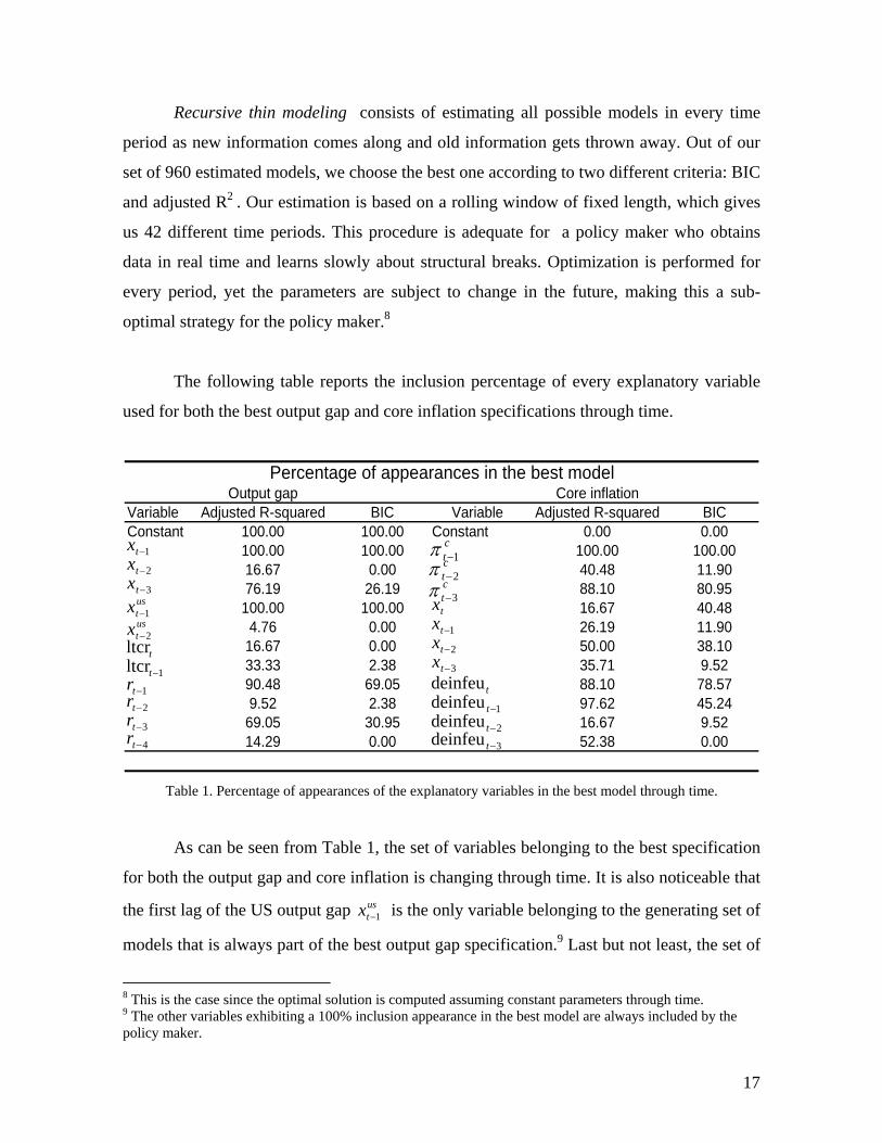
Recursive thin modeling consists of estimating all possible models in every time

period as new information comes along and old information gets thrown away. Out of our

set of 960 estimated models, we choose the best one according to two different criteria: BIC

and adjusted R2 . Our estimation is based on a rolling window of fixed length, which gives

us 42 different time periods. This procedure is adequate for a policy maker who obtains

data in real time and learns slowly about structural breaks. Optimization is performed for

every period, yet the parameters are subject to change in the future, making this a sub-

optimal strategy for the policy maker.8

The following table reports the inclusion percentage of every explanatory variable

used for both the best output gap and core inflation specifications through time.

Output gap Core inflationVariable Adjusted R-squared BIC Variable Adjusted R-squared BICConstant 100.00 100.00 Constant 0.00 0.00

100.00 100.00 100.00 100.0016.67 0.00 40.48 11.9076.19 26.19 88.10 80.95100.00 100.00 16.67 40.48

4.76 0.00 26.19 11.9016.67 0.00 50.00 38.1033.33 2.38 35.71 9.5290.48 69.05 88.10 78.579.52 2.38 97.62 45.24

69.05 30.95 16.67 9.5214.29 0.00 52.38 0.00

Percentage of appearances in the best model

1−tx2−tx3−tx

ustx 1−ustx 2−

tltcr1ltcr −t

1−tr2−tr3−tr4−tr

tx1−tx2−tx3−tx

tdeinfeu1deinfeu −t

2deinfeu −t

3deinfeu −t

ct 1−πct 2−πct 3−π

Table 1. Percentage of appearances of the explanatory variables in the best model through time.

As can be seen from Table 1, the set of variables belonging to the best specification

for both the output gap and core inflation is changing through time. It is also noticeable that

the first lag of the US output gap ustx 1− is the only variable belonging to the generating set of

models that is always part of the best output gap specification.9 Last but not least, the set of

8 This is the case since the optimal solution is computed assuming constant parameters through time. 9 The other variables exhibiting a 100% inclusion appearance in the best model are always included by the policy maker.

18

variables being part of the best specification for both the output gap and core inflation is a

function of the statistical criterion.

The fact that we use a rolling window of fixed length makes it possible to have a

derived optimal policy that responds to either different coefficients when the same

specification arises or different specifications when the set of inclusion variables changes.10

Recursive thick modeling involves estimating all 960 models and taking all of them

into account to deal with the problem of model uncertainty at each point in time. Instead of

choosing just one model, we use two averaging techniques to include the information of all

models. We calculate an average of models with equal weights for each model, and a

weighted average of models, in which weights vary according to the BIC or the 2R

criterion. That is, under this last averaging technique the best models are those with larger

weights.

10 Optimal policies are a function of both the policy maker´s preferences and the dynamic structure of the economy.

19

OPTIMALITY RESULTS VS. ACTUAL NOMINAL RATES The following table shows the results for the six different cases of policy preferences using

the BIC criterion. EW, WA and WM stand for Equal Weights, Weighted Average and

Worst Model, respectively.

As it can be seen from the table above, under thick modeling and the policy maker’s

parameters 3.0,5.0 == φα , the average of all models with equal weights gives us the best

adjustment to the actual data in terms of mean square errors.

Loss Function CETESEW WA WM 28-day rate

Mean Std MSE

Mean Std MSE

Mean Std MSE

Mean Std MSE

Mean Std MSE

6.7357 5.3513

14.1966

8.0175 3.5489

3.0136

7.0634 4.6766

7.6860

10.7419 10.1122

114.6773 7.8888 3.2488

0

6.8192 4.8288

9.4757

7.7772 3.5651

1.8207

7.3234 4.2651

4.734

9.3424 5.4867

29.2125 7.8888 3.2488

0

7.031 4.477

6.4188

7.804 3.515

1.4063

7.5108 4.0264

3.2233

8.9601 4.5682

17.049 7.8888 3.2488

0

6.907 4.6821

8.1879

7.8293 3.5819

1.6208

7.4771 4.1481

3.962

9.2785 5.0435

22.1157 7.8888 3.2488

0

6.7055 5.3144

13.8994

8.1377 3.6837

2.2104

7.3404 4.6996

7.9917

11.3727 9 .0304

93.6 7.8888 3.2488

0

6.7794 5.6046

16.6338

8.6226 3.5705

3.0939

7.4456 4.8436

9.2540

12.0901 12.3514

171.1484 7.8888 3.2488

0

ThickRecursive Thin

Table 2 - Optimal and actual 28-day CETES rate paths: BIC descriptive statistics

21

2 2 * )( ] ) 1 ( ) ( )[ 1 ( −−+ − + − − = tt t ii y L φ α π π α φ

05 . 0 , 5 . 0 = = φ α

2 . 0 , 5 . 0 = = φ α

3 . 0 , 7 . 0 = = φ α

1 . 0 , 9 . 0 = = φ α

05 . 0 , 0 . 1 = = φ α

3 . 0 , 5 . 0 = = φ α

20

The following table statistically compares the difference in mean square errors

among the simple average optimal policies given by some preference parameters. The MSE

obtained with the loss function parameters 3.0,5.0 == φα is statistically different from the

ones obtained with 2.0,5.0 == φα and 3.0,7.0 == φα at the 5% level of significance.

0.0416 0.0359

Table 3:Testing if the difference in mean square errors for simple BIC averages is statistically different from zero

3.0,5.0 == φα2.0,5.0 == φα 3.0,7.0 == φα

The numbers shown are p-values.

We do the same statistical comparison between simple and weighted averages for

the revealed preference parameters. The following table shows that the MSE obtained from

the simple average is statistically lower than the one given by the weighted average.

(Weighted Average)

(Simple Average) 0.0005

Table 4:Testing if the difference in mean square errors between simple and weighted BIC averages is

statistically different from zero

3.0,5.0 == φα

3.0,5.0 == φα

The numbers shown are p-values.

21

The following table shows the results for the six different cases of policy maker’s

preferences using the 2R criterion.

It is important to mention that the simple average of optimal nominal interest rates

here is different from the one obtained for the BIC criterion. This occurs because the

combinations of output gap and core inflation specifications are not the same.11

11 Optimal nominal interest rates are a function of combinations of output gap and core inflation specifications which vary according to the statistical criterion.

Loss Function CETESEW WA WM 28-day rate

Mean Std MSE

Mean Std MSE

Mean StdMSE

Mean Std MSE

Mean Std MSE

6.9038 5.8589

17.1229

7.6350 3.3444

2.4925

7.6198 3.3797

2.4974

7.6654 5.8160

49.9513 7.8888 3.2488

0

7.1764 5.1124

9.9594

7.5869 3.4959

1.7881

7.5787 3.5187

1.8203

7.8268 3.9523

19.9213 7.8888 3.2488

0

7.4377 4.7119

6.5692

7.6659 3.5048

1.4750

7.6619 3.5213

1.4969

7.7712 3.4011

12.6575 7.8888 3.2488

0

7.3566 4.9195

8.3429

7.7071 3.5570

1.5263

7.7015 3.5747

1.5572

7.8307 3.8073

14.7259 7.8888 3.2488

0

7.0699 5.8289

17.6568

7.7812 3.4824

1.9862

7.7699 3.5120

2.0282

7.5360 5 .0275

30.4457 7.8888 3.2488

0

7.1845 6.1656

21.5236

8.1044 3.4507

2.6871

8.0925 3.4844

2.7216

7.8225 6.8220

54.9561 7.8888 3.2488

0

ThickRecursive Thin

Table 5 - Optimal and actual 28-day CETES rate paths: adjusted R-squared descriptive statistics

21

2 2 * )( ] ) 1 ( ) ( )[ 1 ( −−+ − + − − = tt t ii y L φ α π π α φ

05 . 0 , 5 . 0 = = φ α

2 . 0 , 5 . 0 = = φ α

3 . 0 , 7 . 0 = = φ α

1 . 0 , 9 . 0 = = φ α

05 . 0 , 0 . 1 = = φ α

3 . 0 , 5 . 0 = = φ α

22

The following table statistically compares the difference in mean square errors

among the simple average optimal policies given by some preference parameters.

0.0707 0.3996

Table 6:Testing if the difference in mean square errors for simple adj. R2

averages is statistically different from zero

3.0,5.0 == φα2.0,5.0 == φα 3.0,7.0 == φα

The numbers shown are p-values.

Unlike the BIC case, the MSE obtained with the loss function parameters

3.0,5.0 == φα is not statistically different from the one obtained with 3.0,7.0 == φα .

We do the same statistical comparison between simple and weighted averages for the

preference parameters 3.0,5.0 == φα . The following table shows that the MSE obtained

from the simple average is statistically lower than the one given by the weighted average

only at the 10% level of significance.

(Weighted Average)

(Simple Average) 0.0886

Table 7:Testing if the difference in mean square errors between simple and weighted adj. R2 averages

is statistically different from zero

3.0,5.0 == φα

3.0,5.0 == φα

The numbers shown are p-values.

We conclude from the tables above that an equally-weighted average of 960

different models is in any case the best approximation to the interest rate setting behavior of

the policy maker during this period. The results also reveal that the policy maker’s

preferences between stabilizing core inflation around its target and controlling output

variability have been equal. The revealed preferences seem to describe a inflation targeting

regime between flexible and strong with strong interest rate smoothing.

As both Table 2 and Table 5 show, when very little weight is attached to interest

rate smoothing in the loss function of the policy maker (corresponding to cases 1, 5 and 6),

23

the optimal monetary policy derived presents a much larger MSE than in the other cases. In

particular, with preference parameters 3.0,5.0 == φα and 3.0,7.0 == φα the optimal

interest rates obtained under recursive thin modeling and recursive thick modeling have

means and standard deviations closer to those of the actual series.

Last but not least, in following the spirit in Capistrán and Timmermann (2006) to

improve the tracking job of historical nominal rates, we use an affine transformation of the

simple averages. We find no statistical difference between the mean square errors given by

the affine transformation of the simple averages and the simple averages themselves.

CONCLUSIONS

Just like it is done in Favero and Milani (2005), thick modeling is implemented here to deal

with parameter instability and model uncertainty. We find that those problems are relevant

to determining the evolution of the state variables on which monetary policy exerts some

influence. Recursive modeling is complemented with thick modeling in every period in

order to mimic the behavior of an optimal policy maker who takes decisions relying only

on available data up to that point and bearing in mind model uncertainty. The policy maker

takes into account only a very specific type of model uncertainty by making all the possible

combinations from a base set of k regressors. We find the optimal policy rules implied by

each model and take their simple or weighted average according to some statistical

criterion. We find that the implied optimal nominal interest rates for any given period

substantially vary across specifications. Furthermore, we compare the optimal policy

implied by the best model in each period (recursive thin modeling) to simple and weighted

averages of all the optimal nominal rates (recursive thick modeling) in terms of tracking the

historical nominal interest rate in Mexico from January 2001 to June 2004. We are able to

do a better tracking job of the actual nominal interest rates when using averages. These

results argue in favor of making it necessary to take model uncertainty into account when

setting monetary policy.

24

By statistically comparing the MSEs obtained from the average optimal policies

given by different preference parameters, we are able to reveal only a range in which the

revealed preference parameters could be. We do the same statistical comparison between

simple and weighted averages only for the preference parameters 3.0,5.0 == φα . We find

that simple averages work better than weighted averages. The results also show both

reductions in bias and standard deviation in tracking the actual nominal interest rates when

using either simple or weighted averages of optimal nominal interest rates.

The results also indicate that the set of variables belonging to the best specification

for both the output gap and core inflation is changing through time. Last but not least, in

following the spirit in Capistrán and Timmermann (2006) to improve the tracking job of

historical nominal rates, we use an affine transformation of the simple averages obtained

from preference parameters 3.0,5.0 == φα . We find no statistical difference between the

mean square errors given by the affine transformation of the simple averages and the simple

averages themselves.

REFERENCES

Ball, L. (1999). Policy Rules for Open Economies. In J. Taylor (ed.), Monetary

Policy Rules, The University of Chicago Press.

Bossaerts, P. and Hillion, P. (1999). Implementing Statistical Criteria to Select Return

Forecasting Models: What Do We Learn? Review of Financial Studies, 12, 405-428.

Brainard, W. (1967). Uncertainty and the Effectiveness of Policy. American Economic

Review, Papers and Proceedings 57, 411-425.

Capistrán, C. and A. Timmermann. (2006). Affine Transformation of Mean Forecasts: A

Refinement of Equal-Weighted Forecast Combinations, Mimeo, Banco de México

and UCSD.

Contreras M., G. and García S., P. (2002). Estimación de Brecha y Tendencia para la

Economía Chilena. Revista de Economía Chilena, 5(2), 37-55.

Dell´Aquila, R. and Ronchetti, E. (2004). Stock and Bond Return Predictability: The

Discrimination Power of Model Selection Criteria. Université de Genève Working

25

Paper No. 2004.05.

Eichenbaum, M. and Evans, C. (1995). Some Empirical Evidence on the Effects of

Monetary Policy Shocks on Exchange Rates. Quarterly Journal of Economics, 110,

975-1009.

Engert, W. and Selody, J. (1998). Uncertainty and Multiple Paradigms of the Transmission

Mechanism. Bank of Canada Working Paper No. 98-7.

Favero, C. A. and Milani, F. (2005). Parameter Instability, Model Uncertainty and the

Choice of Monetary Policy. B.E. Journals in Macroeconomics: Topics in

Macroeconomics, 5, 1-31.

Giordani, P. and Söderlind, P. (2004). Solution of macro-models with Hansen-Sargent

robust policies: some extensions. Journal of Economic Dynamics and Control, 28,

2367-2397.

Gourinchas, P. and Tornell, A. (1996). Exchange Rate Dynamics and Learning. NBER,

Working Paper No. 5530.

Granger, C.W.J. and Jeon, Y. (2004). Thick modeling. Economic Modelling, 21, 191-385.

Hansen, L. and Sargent, T. (2003). Robust Control and Model Uncertainty in

Macroeconomics. Manuscript, www.stanford.edu/~sargent

Honda, Y. (1982). On Tests of Equality Between Sets of Coefficients in Two Linear

Regressions When Disturbance Variances Are Unequal, The Manchester School, 49,

116- 125.

Jenkins, P. and Longworth, D. (2002). Monetary Policy and Uncertainty. Bank of Canada

Review (Summer): 3-10.

Milani, F. (2003). Monetary Policy with a Wider Information Set: a Bayesian Model

Averaging Approach. Mimeo, Princeton University.

Onatski, A. and Stock, J.H. (2002). Robust monetary policy under model uncertainty in a

small model of the U.S. economy. Macroeconomic Dynamics, 6, 85–110.

Pesaran, M.H. and Timmermann, A. (1995). Predictability of Stock Returns: Robustness

and Economic Significance.

Roldán-Peña, Jéssica (2005). Un Análisis de la Política Monetaria en México bajo el

Esquema de Objetivos de Inflación. Tesis de Licenciatura en Economía, ITAM.

Rudebusch, G.D., and Svensson, L.E.O. (1999). Policy Rules for Inflation Targeting. In J.

26

Taylor (ed.), Monetary Policy Rules, The University of Chicago Press.

Söderström, U. (2002). Monetary Policy with Uncertain Parameters. Scandinavian Journal

of Economics, 104(1), 125-145.

Watt, P. A., (1979). Tests of Equality Between Sets of Coefficients in Two Linear

Regressions When Disturbance Variances Are Unequal: Some Small Sample

Properties, The Manchester School, 47, 391-396.