1

Working Paper Series

Department of Economics

Redistribution and Growth for Poverty Reduction

Hulya Dagdeviran Rolph Van der Hoeven Prof John Weeks Working paper series No. 118 July 2001 ISBN No: 07286 0336 5

2

Word count: approx 9400

Redistribution and

Growth for Poverty Reduction

Hulya Dagdeviren (University of Hertfordshire) Rolph van der Hoeven (ILO)

John Weeks (SOAS) July 2001

Note: Research for this paper was jointly done at ILO and SOAS. Research for this paper was funded by the International Labour Organisation.

3

Redistribution Matters: Growth for Poverty Reduction1 ABSTRACT

In the late 1990s the bilateral and multilateral development agencies placed

increasing emphasis on poverty reduction in developing countries. This emphasis

led to the establishment by the United Nations of the so-called International

Development Targets for poverty reduction. The achievement of a target requires

policies, and policies are most effective within an overall, coherent strategy. A

poverty target might be achieved through faster economic growth alone,

redistribution, or a combination of the two. This paper presents an analytical

framework to assess the effectiveness of growth and redistribution for poverty

reduction. It concludes that redistribution, either of current income or the growth

increment of income, is more effective in reducing poverty for a majority of

countries than growth alone.

1. Introduction

In the late 1990s the bilateral and multilateral development agencies placed

increasing emphasis on poverty reduction in developing countries.2 This emphasis led to

the establishment by the United Nations of the so-called International Development

Targets for poverty reduction. The achievement of a target requires policies, and policies

are most effective within an overall, coherent strategy. By definition a poverty target

might be achieved through economic growth alone, redistribution, or a combination of

the two.

1An earlier version of this paper was presented to the WIDER conference on growth and poverty, May 2001. 2The International Development Targets, set by the Social Summit in 1996, are presented and discussed in Hanmer and Nascold (2000). These were officially adopted by UK Department of International Development (DFID 2000, and Goudie & Ladd 1999). More modest targets were set by USAID (USAID 2001). The new emphasis of the international financial institutions on poverty is reflected in the inclusion of poverty strategies in loan agreements (see IMF & World Bank 1999). For a sceptical view, see Cramer (2000).

4

Setting a specific level of poverty to achieve by a specific date makes comparison

of redistribution and growth analytically interesting. The International Development

Target for ‘head count’ poverty, which we use, was quite specific:

The International Development Target for well-being [of US one dollar per day

per head] is a practical measure of absolute poverty. It is based on an average

of national poverty lines in poor countries, which reflect people’s ability to

afford a diet sufficient to meet minimum nutritional requirements…It thus

represents an internationally agreed operational method of identifying the

number of people who by any standard have unacceptably low incomes.

…

The…target is to reduce by half the proportion of people in developing

countries living in extreme poverty by 2015. The base year is 1990… (DFID

2000, p. 11)

Though the target of fifty percent reduction might be narrowly interpreted as

referring to the developing world as a whole, donor documents treat it as applicable to the

regional and country levels. It may be that for some countries there is no feasible growth

rate, given historical performance, and changes in inequality and resource availabilities

that would achieve it. The World Bank warned that such might be the case:

Progress in reducing extreme poverty during the 1990s was constrained by

increasing inequality in a few countries that accounted for a large share of the

world’s poor. In looking ahead to 2015, continued increases in inequality coupled

with less than robust growth would imply failure to reach the poverty target for

developing countries as a group, and in particular substantial increases in the

number of poor in Sub-Saharan Africa. (World Bank 2001b, p. 7)3

The World Bank went on to conclude that ‘the alternative [growth] scenarios

highlight the importance of achieving fast growth, as well as distributing the benefits of

growth equitably’ (World Bank 2001b, p. 10).4 The same point is made by UK DFID,

3 This document was taken off the internet, without pagination. Page numbers given here are based on numbering form the first pages of text (‘Introduction’). 4 Evidence that the pattern of growth in both developed and developing countries became more unequal is presented in Cornia (1999).

5

‘without growth the poverty reduction large will not be achieved, but it is not enough on

its own’ (DFID 2000, p. 11).5

Despite the wide-spread recognition that GDP growth should be combined with

mechanisms of redistribution to achieve the international poverty target, one finds little

quantitative evaluation of the relative impact of the two poverty determining

mechanisms, either in the abstract or for specific countries; i.e. what would be the

reduction in poverty for a given rate of growth and a given redistribution? Were this

question answered, one could then assess the growth and redistribution mechanisms in

light of the resource cost of their poverty reducing impact.

To calculate the poverty-reducing impact of growth and redistribution, we use a

simple analytical framework that formulates two abstract possibilities: poverty reduction

through distribution-neutral growth (DNG) and poverty reduction through a redistribution

of each period’s growth increment (redistribution with growth, RWG). These are

compared to a conventional one-off redistribution of current income (RCY). Without a

dated poverty target, the question we address, which is more effective for poverty

reduction, growth or redistribution, would be analytically trivial. If a country’s per capita

income lies above the designated poverty line and one ignores the practicalities of

redistribution, poverty can be eliminated by a one-off redistribution in any current time

period, while per capita growth would take several or many periods to achieve the same

result. The imposition of a specific target on the poverty agenda makes our calculations

policy-relevant.

2. Analytical and Policy Framework The evaluation of the effectiveness of growth and distribution for poverty

reduction would be required even were it the case that for the vast majority of countries

historical growth rates would achieve the poverty target (see van der Hoeven 2000). Any

target growth rate, in this case for poverty reduction, has an opportunity cost in foregone

5 For further discussion of the achievability of the targets see Demery & Walton (1998) and Hanmer & Nascold ( 2000).

6

consumption compared to lower rates. This real resource cost can be compared to the

cost of achieving the same poverty reduction at a lower growth rate. Economic growth is

a means, and raising the rate of economic growth without considering the opportunity

cost would be the domestic equivalent of mercantilism.

The relevance of the opportunity cost of raising growth rates passes from

academic to practical interest because, for the vast majority of countries, maintaining

historical growth rates would not be sufficient to meet the international poverty target.6

Table 1, taken from Hanmer and Nascold (2000), demonstrates the inadequacy of past

growth performances for the major developing regions. Only for the East Asia and

Pacific countries was growth above the rate necessary to reach the poverty target. For the

sub-Saharan region, the Middle East and North Africa, and Latin America, both long-run

rates (1965-97) and growth in the 1990s were below what would be required to reach the

poverty target with distribution-neutral growth. In the case of South Asia, a relatively

modest increase on the performance of the 1990s in per capita growth, of about twenty

percent, would be sufficient. Performance for the Central and Eastern European

countries and central Asian countries would be more difficult to assess. The pre-1990

rates were sufficient, but the post-reform performance far below target. It is probably the

case that some of the Central and Eastern European countries would achieve the growth

target, while the central Asian countries could not.

For all the regions the opportunity cost of the target growth rates appears

relevant in light of the substantial degree of income inequality (last column of the table).

To consider this further, an analytical framework is required in which ‘growth’ and

‘redistribution’ are specified rigorously. Using the absolute, internationally comparable

poverty line discussed above, we employ a simple model to generate our empirical

calculations. We define the income distribution of a country over the adult population,

which we divide into percentiles (hi), and the mean income of each percentile is Yi. The

distribution of current income conforms to the following two parameter function:

(1) Yi = Ahiα

6 A discussion of this issue is found in Demery & Walton (1998).

7

Table 1: Growth Rates Required to halve poverty by 2015 and Income Shares

Region Per capita rates:

growth Target

minus*

Item: Region

To meet target

2000-15

Actual

1965-97

Actual

1990-97

Actual 1965-97

Actual

1990-97

Income share, top

20% Sub-Sahara 5.9 -0.2 -0.7 6.1 6.6 52 ME & NA 2.8 0.1 0.7 2.7 2.1 na EAP 3.5 5.4 7.7 -1.9 -2.2 44 South Asia 3.9 2.3 3.3 1.6 0.6 40 LAC 7.0 1.3 2.1 5.7 4.9 53 EE&CA 3.8 3.2 -4.1 0.6 7.9 na Notes: ME&NA – Middle East and North Africa EAP – East and the Pacific LAC – Latin America & the Caribbean EE&CA – Eastern Europe and Central Asia *A negative number indicates that the region grew faster than the rate necessary to meet the poverty target. Sources: Growth rates, Hanmer & Nascold (2000); income share, Deininger & Squire (1996), for the 1990s; and DFID (2000, pp. 16 & 22), where the numbers are reproduced. Similar calculations can be found in World Bank (2000) and World Bank (2001a).

While this function will tend to be inaccurate at the ends of the distribution, its

simplicity allows for a straight-forward demonstration of the interaction between

distribution and growth. Each country’s distribution differs by the degree of inequality

(the parameter α) and the scalar A, which is determined by overall per capita income.

Thus,

(2) A = βYpc

and

(3) Yi = βYpchiα

Total income is, by definition,

(4) Z = mΣβYpchiα for 1 = 1,2...100, and m is the number of people in each

percentile.

8

If the poverty line is Yp = P, we can solve for the percentile in which it falls,

which is also the percentage in poverty (N).7

(5) hp = N = [P/βYpc](1/α)

If we differentiate N with respect to per capita income, we can express the

proportional change in the percentage of the population in poverty in terms of the growth

rate of GDP and the distributional parameters:8

(6) DN/N = n = y[1/α][P/β](1/α)

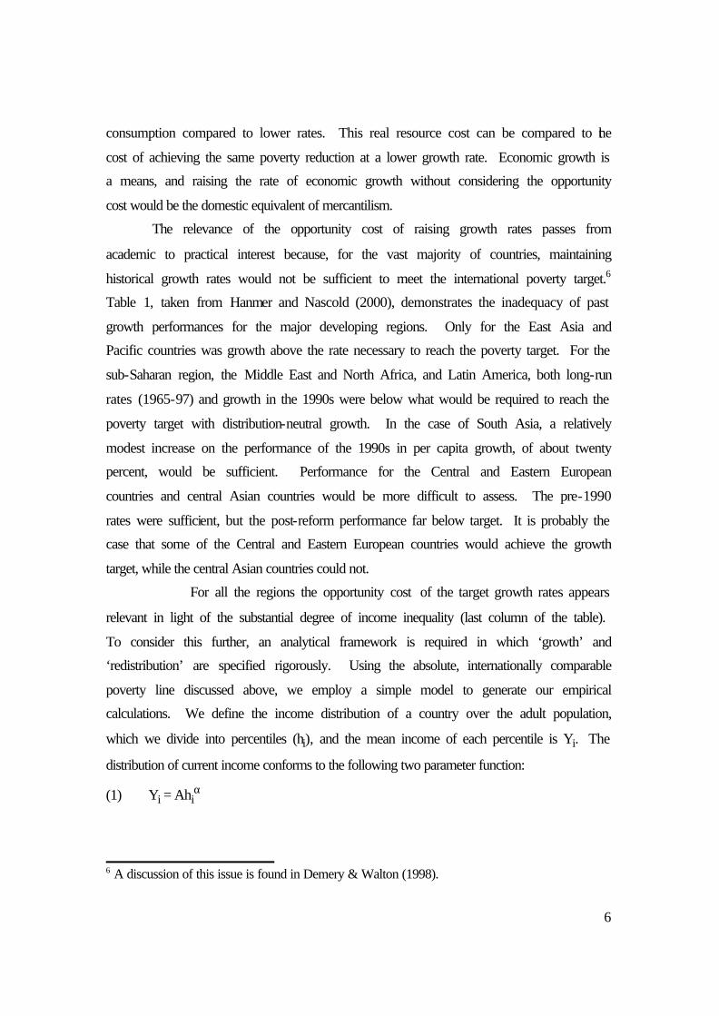
Equation 5 can be used to generate a family of iso-poverty curves, of decreasing

level as they shift to the right, shown in Figure 1, on the assumption that α is constant.

The diagram clarifies the policy alternatives: redistribution of current income involves a

vertical (downward) movement, distribution neutral growth a horizontal (rightward) shift,

and RWG is represented by a vector lying between the two. The diagram implies

generalisations that will be demonstrated by the empirically-based calculations in the

next section. First, because the schedules converge to the left, the impact of

redistribution on poverty declines as per capita income declines. At low incomes, both

redistribution and redistribution with growth are less effective, relatively to distribution

neutral growth. Second, for a given per capita income, the lower the level of inequality,9

the greater is the impact of redistribution on poverty reduction. In other words, when the

poor are clustered close to the poverty line, the income transfer necessary to raise them

out of poverty is less than if the same number of households were unequally distributed.

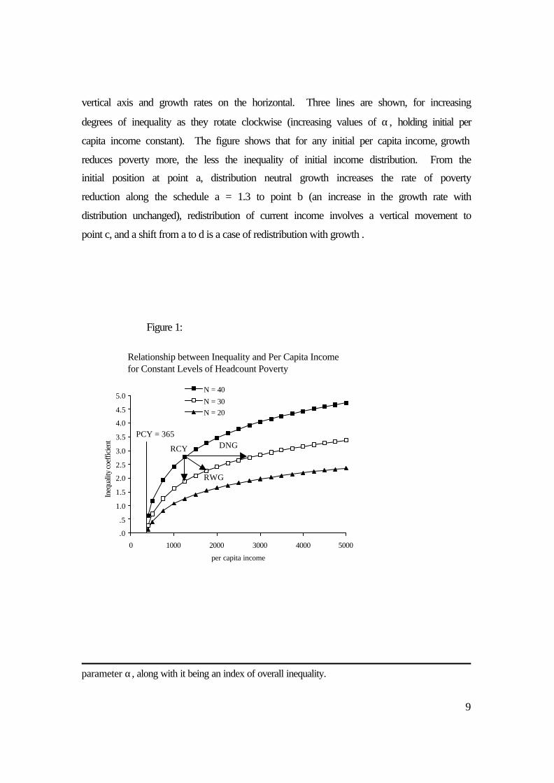
The growth-distribution interaction on poverty reduction can also be shown for

growth rates, using equation 6. In Figure 2, the percentage reduction in poverty is on the

7 A characteristic of this distribution function is that the two parameters, α and β, are not independent of each other. This characteristic does not affect our calculations in the next section, because we use the function only for the initial period’s income. 8 Ravallion (2001, p. 19) proposes that this relationship can be estimated with the simple formula,

n = β(1 – G)y With β an unspecified parameter and G the Gini coefficient of distribution. Using numbers from a number of countries he calculates the value of β, which he calls ‘the elasticity of poverty to growth’. On this basis he obtains a cross-country average for β of –3.74. Since the formula does not specify on what distribution function it is based, it is not clear how one should interpret this so-called elasticity. At most the formula could be considered a rough algorithm for the appropriate relationship among the variables. 9 Our model specifies the slope of the distribution function near the poverty line with the

9

vertical axis and growth rates on the horizontal. Three lines are shown, for increasing

degrees of inequality as they rotate clockwise (increasing values of α, holding initial per

capita income constant). The figure shows that for any initial per capita income, growth

reduces poverty more, the less the inequality of initial income distribution. From the

initial position at point a, distribution neutral growth increases the rate of poverty

reduction along the schedule a = 1.3 to point b (an increase in the growth rate with

distribution unchanged), redistribution of current income involves a vertical movement to

point c, and a shift from a to d is a case of redistribution with growth .

Figure 1:

Relationship between Inequality and Per Capita Income for Constant Levels of Headcount Poverty

.0

.5

1.0

1.5

2.0

2.5

3.0

3.5

4.0

4.5

5.0

0 1000 2000 3000 4000 5000

per capita income

Ineq

ualit

y co

effic

ient

N = 40

N = 30N = 20

DNG

RWG

RCY

PCY = 365

parameter α, along with it being an index of overall inequality.

10

Figure 2:

Poverty Reduction and GDP Growth for Degrees of Inequality

.0

1.0

2.0

3.0

4.0

5.0

6.0

7.0

8.0

9.0

10.0

.0 2.0 4.0 6.0 8.0 10.0

GDP growth rate

% p

over

ty re

duct

ion

α = 1.2

α = 1.3

α = 1.4

DNGRCY

a

bc

RWGd

In anticipation of our empirical calculations, that will show redistribution to be

more effective in reducing poverty than growth for a majority of countries (but not all),

note that using an absolute poverty line has an inherent bias towards the effectiveness of

growth alone (DNG). Assuming all income distributions to be relatively continuous,10

any growth in per capita income, no matter how low, will reduce poverty. However,

redistribution reduces poverty only to the extent that it moves a person above a per capita

income of US$ 365. To put the point another way, redistributions that reduce the degree

of income poverty for those below the absolute poverty standard do not qualify as

poverty reducing.11 Even confronted with this strong condition, we show that simple

10 That is, we assume there are no ‘gaps’ in the distribution below and near the poverty line. 11 A redistribution of one percentage point of GDP from the richest ten percent of the population to the poorest ten percent, equally distributed among the latter, would improve raise the incomes of all those in the lowest decile, but might shift none of them above the poverty line.

11

redistribution rules result in powerful outcomes for poverty reduction. The redistribution

we propose, in the Chenery, et. al. (1974) tradition,12 is equal absolute increments across

all percentiles, top to bottom. This could be viewed as relatively minimalist, with

alternative redistribution rules considerably more progressive.

Assuming that the absence of a distribution policy implies distribution neutral

growth, the proposed equal distribution growth implies income transfers, or an implicit

policy-generated tax. Let aggregate income in the base period be Z0 and in the next

period Z1, and assume the latter is unchanged by how (Z1 – Z0) is distributed across

percentiles.13 With distribution neutral growth the income in each percentile (Yi)

increases by (Y0i[1 + y*]), where y* is the rate of per capita income growth (by

definitional the same across the distirubtion). Under equal distribution growth, each

percentile receives an income increment of (Z1 – Z0)/100. This post-transfer or

secondary distribution of income by percentile is noted as Y1ie, for period 1. Using the

redistribution rule and our symbols,

(7) Z1 = (1 + y*)Z0 = Σ[Y1i], by definition, and

Y1ie = Y0i + {[( y*)Z0]/100} = Y0i + E1

Where Σ[Y1i] = Σ[Y1ie], by definition.

Defining Ti as the implicit redistribution tax for each percentile,

(8) Ti = (Y1i - Y1ie)/(Y1i - Y0i )

The redistribution tax is negative up to the point of mean income (positive income

transfer), then positive above (negative income transfer). If income were normally

distributed, the tax would be negative through the fiftieth percentile. It is obvious that the

more skewed the distribution, the higher is the percentile associated with average per

capita income (the fiftieth percentile being the lower bound). Calculated by percentiles,

12 This volume was path breaking, in that it focused World Bank policy on strategies of poverty reduction. Particularly important were two papers by Ahluwalia (1974a and 1974b), and by Ahluwalia and Chenery (1974a and 1974b). A good review of the distribution literature of the 1960s and 1970s is found in Fields (1980). 13 This assumption is discussed in the section on policy.

12

we find that the redistribution tax is not out of line with rates that have applied in many

developed countries. For example, the extremely unequal Brazilian distribution for the

1990s, with a Gini coefficient of 60,14 implies a marginal tax rate on the hundredth

percentile of slightly more than eighty percent, well below the maximum for such rates in

the United States and Western Europe after World War II, until the early 1960s. Further,

if the redistribution is affected through growth policies rather than direct transfers, the so-

call redistribution tax is implicit rather than levied.

The proposed marginal redistribution has characteristics that derive automatically

from the nature of income distributions. First, and most obvious, the relative benefits of

the equal absolute additions to each income percentile increase as one moves down the

income distribution. Second, and as a result of the first, for any per capita income, the

lower the poverty line, the greater will be the poverty reduction. As a corollary, when a

policy distinction is made between degrees of poverty, with different poverty lines, the

marginal redistribution will reduce ‘severe’ poverty more than it reduces less ‘severe’

poverty. Third, the more unequal the distribution of income below the poverty line, the

less is the reduction in poverty for any increase in per capita income, or redistribution of

that increase.

Before moving to our empirical investigation of alternative growth paths, it is

appropriate briefly to comment on our ‘benchmark’ path, distribution neutral growth.

Dollar and Kray (2000) reach the conclusion, based on cross-country regressions, that the

typical outcome of the growth process in developing countries is to leave the income

share of the lowest quintile unchanged; ie., distribution neutral growth (see also

Ravallion 2001). The authors characterise this with the phrase, ‘growth is good for the

poor’ (italics in the original).15 This statement has limited analytical content, for if the

elasticity of the income share of the poor with respect to growth is positive, ‘growth is

good for the poor’ by definition. Why an elasticity of unity should be the borderline

between growth being ‘good’ or ‘bad’ for the poor is not clear; indeed, it would seem

arbitrary. The policy issue is not whether growth is or is not good for the poor (it is

14 In this paper Gini coefficients will be reported on a scale of zero to one hundred. 15 The same point, that distribution neutral growth appears to be the norm, is demonstrated empirically in a much simpler way and with less fan-fare in Ferreira (1999).

13

except in a few circumstances), but what policy measures can make it better for the poor.

3. Redistribution with Growth: Empirical Calculations

In this section we inspect the impact on poverty in fifty countries of three

calculation exercises, corresponding to different distributional outcomes: 1) a one

percent distribution neutral increase in per capita GDP; 2) a one percent increase in per

capita GDP, distributed equally across income percentiles; and 3) a one percent

redistribution of income from the richest twenty percent to the poorest twenty percent.

The effectiveness of the outcomes in reducing poverty is judged by the time period

required to reduce poverty by a given percentage. This corresponds to the goal of the

International Poverty Targets. In all calculations the US one dollar a day ‘head count’

measure of poverty is used.

The necessary condition for a country to be included in the calculations is that

there were statistics on the income share for quintiles,16 and that the country was included

in the World Bank’s estimates of absolute poverty. The World Bank estimates were

generated by converting each country’s per capita income to constant US dollars for a

base year, then setting a poverty line of US one dollar a day.17 The specified poverty

percentile for one dollar a day is implied by the assumptions made about the distribution

of income within each quintile.

To estimate the impact of a change in income on the percentage of households in

poverty, it is necessary to make explicit the implicit intra-quintile distribution of income.

It was not necessary to know the distribution within all quintiles, but only for the quintile

in which the poverty line fell, before and after the three calculations. Our method implies

the method of estimating the intra-quintile distribution (equation 5). To make the model

more closely conform to each country’s distribution, we let the parameter α vary by

16 The major source was the WIDER income distribution database. See appendix for details by country. 17 The World Bank also provides estimates of the population below two dollars day, but this measure is not used here. The accuracy of these poverty levels is open to criticism (Karshenas 2001). For our purposes this is relatively unimportant, since the conclusions we reach are

14

quintile: α1 applies from the first quintile to the percentile that contains the mean income

of the second quintile, α2 applies from that point to the mean income of the third quintile,

α3 to the mean of the fourth quintile, and α4 for the rest of the distribution. Except for

very low income countries, the poverty line will fall into the first or second quintile, so

only α1 and α2 need be estimated. To estimate those we assume that in the relevant

quintiles mean and median income are equal. Empirical evidence indicates this to be a

close approximation to actual distributions for the bottom two quintiles.18 On this

assumption one can solve for the distribution parameters. If Y(q1m) and Y(q2m) are the

mean incomes of the first and second quintiles (both known), then

(9) Y(q1m) = β1[10.5]α1

Y(q2m) = β2[30.5]α2

One solves for the initial poverty level as above (equation 5).19 After one percent

distribution neutral growth in one time period, the income of that percentile rises by

365x(1.01) = 368.85;

and for equal distribution growth by the increment in aggregate national income equally

distributed across all percentiles (see equation 7). With the income of the initial period’s

poverty line percentile known for the next period, one can calculate the new poverty

percentile (that is, the percentile for which Yi = US$ 365 in the second period).

Having explained the method of calculation, we consider the empirical results.

Table 2 provides the basic statistics for the calculations for the fifty countries: per capita

income, the Gini coefficient, and the percentage of the population with income per head

below one US dollar (the poverty line), as estimated by the World Bank. In Table 3, the

calculations are reported, for the two growth exercises, distribution-neutral growth (DNG

in the table) and equal distribution growth (EDG). Columns one and two give the

relatively insensitive to the exact level of estimated poverty in each country. 18 We are indebted to Malte Lueker for demonstrating this to us, using data from several developing countries. More details can be provided on request. Our calculations are hardly affected by the degree to which the mean and medium incomes differ. 19 The distribution parameters are not sensitive to the difference between mean and median income, unless the difference varies by quintile. The parameter αi is determined by the share of income across quintiles.

15

estimates of the percentile of households lifted out of US one dollar poverty as the result

of one percent growth, distribution-neutral and equal-distribution, respectively. Column

three reports the ‘effectiveness of redistribution’ ratio. This is the ratio of poverty

reduction for equal distribution growth to distribution neutral growth (column 1 divided

by column 2). This ratio is greater than unity for forty-seven of the fifty countries. That

is, for ninety-four percent of the countries, the equal distribution grow strategy reduces

poverty more in a given time period than a distribution-neutral growth strategy. This in

itself is not surprising, for distribution-neutral growth is only more effective in reducing

poverty for countries with fifty percent or more of the population below the poverty line.

It is striking how much more effective equally distributed growth proves to be in

reducing poverty for most countries. For middle income countries the greater

effectiveness of redistribution is quite clear: for a large proportion, the effectiveness ratio

is in excess of three; ie., equal distribution growth raises three times as many households

from poverty than distribution neutral growth over any time period.

The benefits of equal distribution growth are greater the higher is a country’s per

capita income, and the more equal the distribution below the poverty line. The results

imply that growth with redistribution would be particularly appropriate for the Latin

American countries and those of North Africa and the Middle East. Its poverty-reducing

advantage would be less for the sub-Saharan countries (except South Africa), because of

their low per capita incomes. Because the table includes only a few low-income

countries, it overstates the proportion of countries for which redistribution with growth is

more effective than distribution neutral growth. This over-emphasis is discussed below.

As the poverty line rises up a country’s income distribution, the effectiveness of

redistribution ratio becomes less and less sensitive to measures of inequality. However,

it is always the case, no matter what a country’s per capita income or degree of

inequality,20 that redistribution with growth is more effective than distribution neutral

growth in reducing the intensity of poverty (as opposed to the head count). The relative

benefit of equal distribution growth increases as one moves down the income

distribution, independently of a country’s per capita income or degree of inequality.21

20 That is, for any distribution that is not equal. 21 However, in the 1990s inequality increased dramatically in most of these countries (Brundenius

16

The redistribution with growth outcome implies a tax on all households whose

income is above the mean. In which percentile the mean falls depends on the skewedness

of the distribution. The final two columns (4 and 5) of Table 3 report the implied tax rate

for the highest percentile, and the average rate across all percentiles whose income is

redistributed towards the poorer percentiles. This calculation presents the issue of the

effect of the redistribution on incentives of positive and negative transfers.22 If

distribution neutral growth represents the primary (pre-tax) outcome, and equal-

distribution growth the secondary (post-tax) outcome, then there is a straight-forward

disincentive effect for those taxed, to be weighted against the incentive effect for the

beneficiaries. We make the assumption that the incentive effect of taxes is symmetrical:

if positive tax rates create a disincentive to earn further income, then negative rates create

an incentive to earn income and contribute to higher national growth. If the income

distribution is skewed, then the number of households enjoying an incentive to increase

earnings will out-number those suffering a disincentive, and the impact on growth should

be positive. Whether this increases or decreases the growth rate would depend on the

income-weighted average of the incentive effects.

These growth calculations can be compared to the more conventional exercise, a

direct redistribution from the rich to the poor. This is calculated in Table 4, where it is

assumed that one percentage point of total national income is shifted from the top quintile

to the poor, and distributed equally among those households.23 This assumption is

equivalent to assuming that a one percent increase in GDP goes to those below the

poverty line. For each country the reduction in the poverty measure for the one percent

redistribution appears in column two, and can be compared to column three in Table 2,

where poverty prior to redistribution is given. The outcome is summarised in column

three of Table 4, which reports the percentage reduction in poverty as the result of the

redistribution. For example, pre-redistribution poverty in Brazil was measured as 23.2

percent of the population, and is simulated to be 18.4 percent after redistribution, for a

and Weeks 2001), marking them more like the Latin American group for purposes of poverty reduction analysis. 22 The rates are marginal, not average, applying to the increase or growth increment in per capita income. 23 At the poverty boundary, this redistribution shifts some households above the ones with slightly

17

fall of 20.7 percent (4.8 percentage points). The final column of the table gives the

implicit tax rates on the highest quintile resulting from the redistribution. These prove to

be quite low, varying from less than two percent to a high of three percent, inversely

related to inequality (ie., the share of income accruing to the top quintile before

redistribution).

The poverty reductions associated with redistribution of current income vary

dramatically across countries. In general, the lower the per capita income of a country,

the less is the poverty reduction. This is demonstrated most obviously for the twelve

Latin American countries, among which the reduction for the Central American states

and Ecuador is virtually nil. The other obvious influence is inequality. The lower the

inequality just below the poverty line, holding per capita income constant, the greater the

poverty reduction from a redistribution, because those below the poverty line are

‘packed’ close together. Comparing the middle-income Latin American countries to the

former centrally planned countries reveals this.

These results suggest a typology of countries differentiated by the general strategy

that is most conducive to poverty reduction, and this is done in Table 5. Columns two

and three give the number of years required for distribution neutral growth and equal

distribution growth to achieve the same poverty reduction as a transfer of one percent of

national income from the highest to the lowest quintile. To take the first country,

Venezuela, distribution neutral growth would require over thirty-four years to reduce

poverty by the same amount as the one percentage point redistribution, and equal

distribution growth would require six years. On the basis of these calculations, the fifty

countries fall into three categories. In category 1, the ‘income redistribution countries’,

both growth strategies require more than one year to reduce poverty as much as a straight

redistribution. The countries are listed in descending order of the number of years

required for distribution-neutral growth to match the impact of the one percent

redistribution on poverty. For thirty-four of the fifty countries (sixty-eight percent),

straight redistribution is the most effective method of poverty reduction.

In category 2 are thirteen ‘redistribution with growth’ countries, for which

redistribution is not the most effective poverty reduction strategy, and equal distribution

higher pre-redistribution incomes, but this does not affect the conclusions reached in the text.

18

growth is more effective than distribution-neutral growth. This is emphasised by

inclusion of the ‘effectiveness ratio’ in the final column (taken from Table 3). These

countries are characterised either by low per capita income or relatively equal distribution

(or some combination of the two). Finally, there is category 3, three ‘trickle down’

countries, for which growth as such is the most effective vehicle for poverty reduction.

The defining characteristic of the trickle down countries is that they have more than fifty

percent of their population in poverty as a result of their low per capita income.

However, it does not follow that all low income countries would fall into this category. If

low income is combined with a relatively equal distribution, as for Niger, equal

distribution growth may be more effective in reducing poverty, if only marginally so in

that specific case.

The calculations demonstrate that for the majority of middle-income countries,

poverty reduction is most effectively achieved by a redistribution of current income. For

the same countries, redistribution with growth would be the second-best option, and

distribution neutral, or status quo growth, a poor third. Figure 3 demonstrates the

relationship between the three poverty strategies and levels of per capita income, for a

given level of overall inequality. The graph is constructed using a regression algorithm

and the fifty countries in our tables. For each country, the number of years required for

distribution neutral growth or redistribution with growth to achieve the same poverty

reduction as redistribution of current income is estimated as function of per capita income

and the Gini coefficient. The regression equations are only a rough approximation, since

the Gini is a crude proxy for the slope of the distribution function just below the poverty

line (implied by the parameter α in our model).24 Using the regressions, two curves are

shown, for DNG and RWG, respectively, for a Gini of 40 (close to the average value

24 The regression algorithms are as follows, where A(DNG) and A(EDG) are the number of years to achieve the equivalent of a redistribution of current income, PCY is per capita income, and G is the Gini coefficient. The significance of coefficients is given in parenthesis below the coefficients, and relevant other statistics below them. A(DNG) = -79.08 + 10.77ln(PCY) + 3.55ln(G) (.01) (.01) (.10) R2 = .47 F = 19.8 N = 47 A(EDG) = -6.38 + 2.91ln(PCY) – 2.94ln(G) (nsgn) (.01) (.01)

19

across the fifty countries). DNG and RWG are judged as less effective than

redistribution of current income if they require more than one year to achieve the same

percentage point reduction in poverty.

The graph indicates that redistribution with growth becomes more effective when

per capita income falls below about US$ 700, and distribution neutral growth replaces it

as most effective when per capita income drops below about US$ 450. While the curves

are only indicative (inequality varies across countries), they demonstrate the following

general points: 1) for middle-income countries redistribution of current income is the

most effective method of poverty reduction; 2) for very low income countries,

distribution neutral growth is most effective, and 3) the per capita income range for

which redistribution with growth is most effective is quite narrow, though it is more

effective than DNG except at very low per capita incomes.

In principle, the analogue used to generate Figure 3 could be employed to divide

all countries as we have done for the fifty in Table 5. However, this cannot be done with

only precision in practice, due to lack of distributional data and the problem of measuring

consistently per capita income across countries and over time. A very rough estimate of

the number of countries in the three categories is possible. If we assume that the Gini

coefficients for the countries not in Table 5 lie between 40 and 50, the relevant

‘borderline’ countries are Senegal (lowest among the redistribution of current income

countries) and Niger (lowest among the redistribution with growth countries). We order

all developing countries by per capita income using the latest World Bank World

Development Indicators (data for 1999), and treat these two countries as the appropriate

boundaries for the three categories of poverty reduction strategies. Using this rough

method, of 132 developing countries the count is the following: redistribution of current

income would be most effective for sixty-five; redistribution with growth for twenty; and

distribution neutral growth for the remaining forty-seven. If a political judgement

rejected redistribution of current income, then two-thirds of the countries should, on

technical grounds, pursue a poverty reduction strategy that purposefully seeks to alter the

distribution of the increment in growth. These eighty or more countries include all the

middle-income countries, almost all the European and Asian countries in transition, and

R2 = .49 F = 20.1 N = 47

20

many of the low-income countries. On the other hand, for almost all countries in the

United Nations category of Least Developed Countries a distribution neutral growth path

would be the most poverty reducing. With these generalisations in mind, we consider

poverty reduction policies in the following section.

Figure 3

Effectiveness of Poverty Reduction Strategies, NDG & RWG, for Given Levels of Inequality (from cross-country regression)

-5

-3

-1

1

3

5

7

9

11

13

15

0 500 1000 1500 2000

per capita income

year

s to

equ

al R

CY

= 1

%

DNG(g=40)

RWG(g=40)

DNG

RWG

RCY

A B

Years = 1

A = US$ 450B = US$ 700

5. Policy Effectiveness for Redistribution with Growth

The major element required to introduce and effectively implement a re-

distributive strategy in any country is the construction of a broad political coalition for

poverty reduction (see Bell 1974). The task of this coalition would be the formidable one

21

of pressuring governments for redistribution policies, while neutralising opposition to

those policies from groups whose self-interest rests with the status quo. How such a

political coalition might come about is specific to each country and its discussion beyond

the scope of this paper. We focus on a less fundamental, but crucially practical issue: the

policies that could bring about a redistribution strategy. To be policy relevant, our

consideration of redistribution mechanisms must move beyond a listing of possibilities to

an analysis of the likely effectiveness of these.

First, the question of effectiveness should be considered on the macro level, by

returning to the question raised in the first section: what are the opportunity costs of

reducing poverty by increasing the growth rate and implementing redistribution? The

opportunity cost of implementation will be determined by the specifics of the programme

to achieve redistribution, the size of the redistribution, and the administrative capacity of

the public sector. None of these can be determined in the abstract. However, the

opportunity cost of raising the growth rate can be quantified within broad limits. From

equation six, we have:

n = y[1/α][P/β](1/a)

And the consumption foregone to achieve any growth rate y is determined by the

familiar equation, y = sv, where s is the net saving rate and v is the output-capital ratio.

The opportunity cost of lowering poverty through growth alone can be indicated using

the calculations for the Latin American countries. Table 3 shows that a distribution

neutral growth rate of one percent reduces poverty by .32 percentage points, while equal

distribution growth would achieve the same reduction with a growth rate of .26

percentage points. To double the distribution neutral growth reduction of poverty would

require an increase of the saving rate of the amount (1/v). If the capital-output ratio is

approximately four, then increasing the annual rate of poverty reduction by one

percentage point calls for an increase in the saving rate of four percentage points. Equal

distribution growth would achieve the same poverty reduction with one percentage point

increase in the saving rate. The difference in the required changes in the saving rate

implies that equal distribution growth would have a substantially lower opportunity cost

of poverty reduction (three percentage points of GDP).

22

Therefore, equal distribution growth would be a more economically efficient way

to reduce poverty as long as its administrative cost did not exceed three percentage points

of GDP. To continue with the an example for the Latin American region, equal

distribution growth would involve redistributing half of one percent of national income

for period two (after one percent EDG). If this small redistribution could be achieved

with an administrative outlay of less than three percentage points of national income, an

extravagant upper little to the administrative cost ratio of six-to-one, then EDG would be

more effective than DNG.

The opportunity cost of the two growth patterns is demonstrated in Figure 4. The

increase in the saving rate required to raise the growth rate one percentage point is equal

to the capital-output ratio. As an approximation, it is assumed that the capita-output ratio

is an increasing function of per capita income. Specifically, it is assumed that the ratio is

three for the poorest country of the fifty (Zambia with per capita income of US$210 in

1993) and 4.5 for the country with the richest (Thailand at US$2570 in 1992), and

increases linearly with per capita income. This, shown by the straight line DNG, is

compared to increase in the saving ratio for the equal distribution growth rate that

generates the same percentage point poverty reduction (which can be calculated from

Table 3). For all but nine countries (noted in the chart), the ‘savings gap’ between DNG

and EDG increases with per capita income. Seven of the nine were countries in transition

from central planning, with low initial poverty and/or low inequality. We can

summarise: 1) the opportunity cost of lowering poverty through growth alone rises with

per capita income; and 2) the likelihood that the administrative costs of redistribution

would render EDG as or more expensive than DNG also decreases with per capita

income. In conclusion, arguments that assert that redistribution to be ‘too expensive’

appear unfounded when one that considers the opportunity cost of reducing poverty

through growth alone.25

25 For any particular programme, administrative costs would have to be carefully calculated and compared to those of alternative policies. There is relatively little work on this topic. For a case

23

Figure 4

Rise in the Saving Rate for One Percent DNG and for Poverty-reduction Equivalent EDG (by country & per capita income)

0

0.5

1

1.5

2

2.5

3

3.5

4

4.5

5

0 500 1000 1500 2000 2500 3000

per capita income

chan

ge in

S/Y

DNG

EDG

ThailandRussia

KazakhstanCzech Rep

Lithuania

Slovak Rep

Hungary

Lesotho

Belarus

Turning to specific measures for redistribution, perhaps the most important

determinant of the effectiveness of the various measures and specifics of each

redistribution strategy is the structure of an economy. This structure will depend on the

level of development, which will to a great extent condition the country’s production

mix, the endowments of socio-economic groups, the remuneration to factors, direct and

indirect taxes on income and assets, prices paid for goods and services, and transfer

payments. These elements of the distribution system are initial conditions that delineate

the scope for redistributive policies. In this analytical context, the implementation

study, see Grosh (1995).

24

requirements of redistributive policies can be summarised in a simple algebraic

framework (see Hanmer et.al. 1997). Define the following terms:

Y denotes the income of a household, V is transfer payments, T is taxes, k is a

vector of assets (including human capital), w is a vector of rates of return

(including wages), p is the price vector of goods and services, q is the quantity

vector of those goods and services, and S is household saving.

Then, by definition,

Y = (V – T) + wk = pq + S

Transfer payments (unemployment compensation, pensions, child benefits, aid to disabled) & progressive taxes (on income and wealth) Effective in middle-income countries

Minimum wages, low-wage subsidies, other labour market regulations, public employment schemes (w); credit programmes for the poor; land reform, education (k); Effective in middle-income and some low-income countries

Subsidies for basic needs goods, public sector infra-structure invest-ment (p); child nutrition programmes (q) Effective in most countries

Facilitate future asset acquisition: ‘village banks’ & other financial services for the poor Effective in most countries

The effectiveness of tax and expenditure policies (V and T) to generate secondary

and tertiary distributions more equitable than the primary distribution depends upon the

relative importance of the formal sector.26 This is for the obvious reason that

governments can most effectively apply progressive income taxes to wage employees and

corporations. All empirical evidence shows that the formal sector wage bill and profit

shares increase with the level of development. Along with the importance of the formal

sector goes a high degree of urbanisation, and working-poor urban households are more

easily targeted than either the rural poor or urban informal sector households. The

experience of a number of middle-income countries has demonstrated the effectiveness of

basic income payments for poverty reduction, with an example being the basic pension

paid to the elderly in South Africa.27

26 For a review of fiscal policies for redistribution, see Chu, Davoodi & Gupta 1999). 27 While relatively low, the pension in the 1990s was an important income source for the rural

25

As shown in the previous section, the redistribution strategy is most appropriate

for middle-income countries, because their per capita incomes are high relatively to the

absolute poverty line. These are also the countries whose economic structures make

taxation and expenditure instruments effective for redistribution. Thus, the thirty-seven

‘income redistribution’ countries, and others at similar levels of development, qualify for

the redistributive strategy via income and corporate taxes, both in terms of its intrinsic

effectiveness and the institutional capacity to implement it. Such countries would include

the larger ones in Latin America (Argentina, Brazil, Chile, Mexico and Venezuela),

several Asian countries (the Republic of Korea, Thailand, and Malaysia), and virtually all

former socialist countries of Central and Eastern Europe.

To a certain extent, specific economic structures allow for effective use of

taxation for redistribution in a few low-income countries that would typically be relevant

only for middle-income countries. If the economy of a low-income country is dominated

by petroleum or mineral production, then modern sector corporations may generate a

large portion of national income. This allows for effective taxation even though

administrative capacity of the public sector may be limited. The tax revenue can be

redistributed through poverty-reduction programmes, though not through transfer

payments if the labour force is predominantly rural. Examples of mineral-rich low-

income countries with the potential to have done this, albeit unrealised, were Nigeria,

Liberia, and Zambia.

Interventions to change the distribution of earned income (wk in the equation

above), which alter market outcomes, will also tend to be more effective in middle-

income countries (ILO 1992). The most common intervention is a minimum wage,

though there are many other policies to improve earnings from work (see Rogers 1995).

Further mechanisms include public employment schemes and tax subsidies to enterprises

to hire low-wage labour. It is unlikely that any of these would be effective in low-income

countries, because of enforcement problems (minimum wage), targeting difficulties

(employment schemes), and narrowness of impact (wage subsidies).

Land reform might achieve poverty reduction for rural households, but the

relationship between land redistribution and level of development is a complex one. On

poor, especially for female-headed households (see Standing, Sender and Weeks 1996, Chap 6).

26

the one hand, low-income countries are predominantly rural, so if land ownership is

concentrated, its redistribution could have a substantial impact on poverty. Further, the

more underdeveloped a country, the less commercialised tend to be poor rural

households. Therefore, the benefits to the poor from land redistribution in low-income

countries are less likely to be contingent on support services. On the other hand, lack of

administrative capacity and so-called traditional tenure systems represent substantial

constraints to land redistribution in many low-income countries, and especially in the

sub-Saharan countries. The usual approach to land redistribution presupposes private

ownership, such that it is clear from whom the land will be taken and to whom it will be

given. There are few sub-Saharan countries in which private ownership is widespread,

making redistribution difficult or impossible without prior clarification of ownership

claims (Platteau 1992, 1995). While land redistribution is probably not an effective

poverty reducing measure for most low-income countries, a few notable exceptions in

Asia (e.g., India and Vietnam) suggest that it should not be ruled out in all cases.

For middle-income countries, experience in Latin America has shown that

governments can effectively implement land redistribution, though subsequent poverty

reduction is dependent on provision of rural support services (Thiesenhusen 1989).

However, the high degree of commercialisation of agriculture in middle-income countries

requires that redistribution be complemented by a range of rural support services,

including agricultural extension, marketing facilities, and other measures. Perhaps more

serious, the relevance of land reform for poverty reduction tends to decline as countries

develop and the rural population shrinks relatively and absolutely. For example, at the

end of the twentieth century in the five most populous Latin American countries, twenty

percent or less of the labour force was in agriculture. Minimum wages may be more

relevant than land redistribution in reducing poverty among the landless and near-

landless in such countries.28

Interventions that directly affect the prices and access to goods and services (pq)

could potentially be quite powerful instruments for poverty reduction. Subsidies to

selected commodities have the administrative advantage of not requiring targeting, only

28 This is particularly the case if there are no output gains from land redistribution; i.e., if the so-called inverse size rule does not hold (see Dyer 1997).

27

identification of those items that carry a large weight in the expenditure of the poor.

While multilateral adjustment programmes typically require an end to such subsidies on

grounds of allocative efficiency or excessive budgetary cost, the rules of the World Trade

Organisation do not, as long as subsidies do not discriminate between domestic

production and imports (FAO 1998). Whether subsidies would generate excessive fiscal

strain would depend on the products covered and financing. Again, the level of

development of a country is of central importance for the effectiveness of subsidies. In

low-income countries with the majority of the poor in the countryside, consumer

subsidies are unlikely to have a significant impact on the poor outside urban areas. Basic

goods provision in kind can be an effective instrument for poverty reduction even in very

low-income countries, by delivering such items as milk to school children. To do so with

a non-targeted programme would require a progressive tax system, which would be more

likely in a middle-income country.

In all countries the poor suffer from poor health and inadequate education

relatively to the non-poor. Expenditures on education and health have the practical

advantage that programmes that would help the poor are easily identified, though the

specifics would vary by country. However, providing these services to the poor may in

some countries be as politically difficult as more obviously controversial measures such

as asset redistribution. The same point applies to infrastructure programmes directed to

poverty reduction. To the extent that these would reduce public investment in projects

favoured by the non-poor, especially the wealthy, they may be no easier to implement

that measures that appear superficially to be more radical.

Table 6 provides a summary of the discussion, with poverty-reducing measures

listed by rows, and the three categories of countries across columns. The table indicates

that for the ‘redistribution’ countries, a redistribution of current income and assets is the

most effective means of poverty reduction, and the methods to achieve this are feasible.

For the ‘redistribution with growth’ countries, the measures for redistribution of current

income and assets are less feasible, but instruments to achieve the more modest goal of

redistributing the growth increment would be feasible. Finally, most redistribution

instruments would not be feasible, or only to a limited degree, for very low-income

28

countries; but for these countries, a growth strategy with no redistributive mechanisms

may be the most poverty-reducing path.

This discussion indicates that implementing an agenda of redistribution involves

major problems, but these problems should not be exaggerated. In many countries they

might prove no more intractable than the problems associated with implementation of

other economic policies. An effective orthodox monetary policy is difficult to implement

if a country is too small or underdeveloped to have a bond market. The absence of a

bond market leaves the monetary authorities unable to ‘sterilise’ foreign exchange flows.

Similarly, replacing tariffs by a value added tax would be a daunting task in a country

whose commerce was primarily through small traders. Lack of public sector capacity

would limit the ability to execute a range of so-called supply side policies: privatisation,

‘transparency’ mechanisms’, and decentralisation of central government service delivery

(van der Hoeven and van der Geest 1999). The multilateral agencies have recognised

these constraints to adjustment programmes, and typically made the decision that

constrained implemented was preferable to non-implementation. The same argument can

be made for a redistributive growth strategy: to achieve poverty reduction, it might

preferable to implement re-distributive growth imperfectly than to implement the status

quo imperfectly.

Table 6: Summary of Feasibility of Redistribution Instruments by Category of Country

Country Category:

Redistributive Instrument:

Redistribution of current income & assets

(middle-income countries)

Growth with redistribution policies (middle & most low-income countries)

Growth without redistribution policies

(very low-income countries)

Progressive taxation

Yes

Yes for some countries

No

Transfer payments

Yes

Yes for some countries

No

Consumer subsidies

Yes

Yes

Yes for some countries

Land reform

Yes, but not always relevant

Yes

Not for most countries

Education & health

Yes

Yes

Yes

Infrastructure & public works

Yes

Yes

Yes

29

6. Conclusion

Poverty reduction has always been a priority of development policy, albeit

sometimes only at the rhetorical level. The end of the 1990s brought increased emphasis

on bringing the benefits of growth to the poor (Rodrik 1994, Alesina 1998, Bruno,

Ravallion & Squire 1998). However, growth alone is a rather blunt instrument for

poverty reduction, since the consensus of empirical work suggests that it is distribution

neutral. Along with emphasis on poverty reduction, a shift occurred in the policy

literature towards a more favourable view of policies to redistribution income and assets.

An integration of distributional concerns and a priority on poverty reduction could be the

basis for a new policy agenda to foster both growth and equity.

This new agenda would be based on three analytical generalisations: 1) that

greater distributional equality provides a favourable ‘initial condition’ for rapid and

sustainable growth; 2) that redistribution of current income and assets, or redistribution

of an economy’s growth increment is the most effective forms of poverty reduction for

most countries; 3) the mechanisms to achieve the redistributions are feasible for most

countries; and 4) the administrative costs of these mechanisms are highly unlikely to

cancel out the gains in poverty reduction. These generalisations imply that the new

agenda could focus upon specific policies and instruments of redistribution, with the goal

of substantial reductions in urban and rural poverty in the medium term.

30

REFERENCES

Ahluwalia, M. S. 1974a “Income Inequality: Some Dimensions of the Problem” in Redistribution

with Growth by H. Chenery, M. S. Ahluwalia, C. L. G. Bell, J. H. Duloy and R. Jolly, (Oxford: Oxford University Press) pp. 3-37

1974b “The Scope For Policy Intervention”, in Redistribution with Growth by H. Chenery, M. S. Ahluwalia, C. L. G. Bell, J. H. Duloy and R. Jolly, Chapter IV, (Oxford: Oxford University Press) pp. 73-90

Ahluwalia, M. S.; Chenery, H. 1974a “The Economic Framework”, in Redistribution with Growth by H.

Chenery, M. S. Ahluwalia, C. L. G. Bell, J. H. Duloy and R. Jolly, Chapter II, (Oxford: Oxford University Press) pp. 38-51

1974b “A Model of Redistribution and Growth”, in Redistribution with Growth by H. Chenery, M. S. Ahluwalia, C. L. G. Bell, J. H. Duloy and R. Jolly, (Oxford: Oxford University Press) pp. 209-235

Alesina, A. 1998 “The Political Economy of Macroeconomic Stabilizations and Income

Inequality: Myths and Reality” in Income Distribution and High-Quality Growth, V. Tanzi and K. Chu (eds.), (Cambridge, Mass: MIT Press) pp. 299-326.

Rodrik, D. 1994 “Distributive Politics and Economic Growth”, Quarterly Journal of

Economics, Vol. 109, No.2, pp. 465-490 Bell, C. L. G. 1974 “The Political Framework” in Redistribution with Growth by H. Chenery,

M. S. Ahluwalia, C. L. G. Bell, J. H. Duloy and R. Jolly, Chapter V, (Oxford: Oxford University Press)

Brundenius, Claes, and Weeks, John 2001 “Globalization and Third World Socialism,” in Claes Brundenius and John

Weeks (eds.), Globalization and Third World Socialism: Cuba and Vietnam (London: Palgrave)

Chenery, H., M. S. Ahluwalia, C. L. G. Bell, J. H. Duloy and R. Jolly (Chenery, et. al.) 1974 Redistribution with Growth (Oxford: Oxford University Press) Chu, K.; Davoodi, H.; Gupta, S 1999 “Income Distribution and Tax and Government Spending Policies in

Developing Countries”, Draft Paper Prepared for WIDER Project Meeting on Rising Income Inequality and Poverty Reduction, 16-18 July 1999, Helsinki

Cornia, G. A. 1999 “Liberalization, Globalization and Income Distribution”, WIDER Working

Paper Series, No. 157, March 1999 Cornia, G. A.; Reddy, S. 1999 “The Impact of Adjustment Related Social Funds on Distribution and

Poverty”, WIDER Project Meeting on Rising Income Inequality and Poverty Reduction, 16-18 July 1999, Helsinki

31

Cramer, Chris 2000 “Inequality, Development and Economic Correctness,” SOAS Department

of Economics Working Paper no.105, November 2000. Deininger, K., and L. Squire 1996 ‘A New Data Set Measuring Income Inequality,’ World Bank Economic

Review 10, pp. 565-592 Demery, L., and M. Walton 1998 ‘Are Poverty and Social Goals for the 21st Century Attainable?’ IDS

Bulletin, 30 Department for International Development (UK) 1997 Eliminating World Poverty: A challenge for the 21st Century (London:

The Stationery Office) 2000 Halving world poverty by 2015: Economic growth, equity and security

(London: DFID) Dollar, David, and Aart Kray 2000 ‘Growth is Good for the Poor,’ (www.worldbank.org/research: World

Bank) Dyer, Graham 1997 Class, State and Agricultural Productivity in Egypt. A Study of the Inverse

Relationship between Farm Size and Land Productivity, (London: Frank Cass) Fields, Gary 1980 Poverty, Inequality and Development (Cambridge: Cambridge University

Press) Ferreira, Francisco H. G. 1999 “Inequality and Economic Performance,’ (www. worldbank.org/poverty/ inequal/index.htm: World Bank) Food and Agricultural Organisation, Statistics Division 1998 The implications of the Uruguay Round Agreement on Agriculture for

Developing Countries, Training Materials for Agricultural Planning 41 (Rome: FAO)

Goudie, Andrew, and Paul Ladd 1999 ‘Economic Growth, Poverty and Inequality,’ Journal of International

Development 11,2, pp. 177-195 Grosh, M. E. 1995 “Towards Quantifying the Trade-off: Administrative Costs and Incidence in

Targeted Programs in Latin America”, in Public Spending and the Poor, , D. van de Walle and K. Neat (eds.), (Baltimore: John Hopkins University Press for the World Bank) pp. 450-88.

Hanmer, L., and F. Nascold 2000 ‘Attaining the International Development Targets: Will growth be enough?’

Development Policy Review 18, 1, pp. 11-36 International Fund for Agricultural Development (IFAD) 1999 “Rural Poverty: A Regional Assessment”, International Fund for

Agricultural Development, Latin America and Caribbean Division, September

32

International Labour Organisation (ILO) 1992 Incomes Policies in the Wider Context: Wage, Price and Fiscal Initiatives in

Developing Countries, F. Paukert and D. Robinson (eds.), 1992, Geneva: International Labour Office

IMF and The World Bank 1999 Poverty Reduction Strategy Papers: Operational Issues, (Washington:

World Bank) Kanbur, R. 1999 “Income Distribution and Growth”, World Bank Working Papers: 98-13,

Washington, D. C.: The World Bank Kanbur, R.; Squire, L. 1999 “The Evolution of Thinking about Poverty: Exploring the Interactions”

mimeographed document , World Development Report Office , Washington D.C. World Bank

Karshenas, Massoud 2001 “Measurement of Absolute Poverty in Least Developed Countries (LDCs),”

SOAS Department of Economics Working Paper (London: School of African and Asian Studies))

Platteau, Jean-Philippe 1992 “Land Reform and Structural Adjustment in sub-Saharan Africa:

controversies and guidelines,” FAO Economic and Social Development Paper 107 (Rome: FAO)

1995 Reforming Land Rights in Sub-Saharan Africa: Issues of Efficiency and Equity, Research Institute for Social Development, Discussion Paper 60 (Geneva:

Psacharopoulis, George, Samuel Morley, Ariel Fiszbein, and Bill Wood 1996 Poverty and Income Distribution in Latin America: The story of the 1980s,

World Bank Technical Paper No. 351 (Washington: World Bank) Ravallion, M. 2001 ‘Growth, Inequality and Poverty: Looking beyond averages,’

UNU/WIDER Development Conference on Growth and Poverty, Helsinki, 25-26 May

Standing, Guy, Sender, John and Weeks, John 1996 Restructuring the Labour Market: The South African Challenge (Geneva:

ILO) Thiesenhusen, W. H. 1989 Searching for Agrarian Reform in Latin America (Winchester, MA:

Unwin Hyman) van der Hoeven, R. 2000 “Poverty and Structural Adjustment. Some Remarks on the Trade-off

between Equity and Growth,” in New Poverty Strategies, What have they achieved, What have we learned? P. Mosley and A. Booth (eds.) ( London Macmillan).

van der Hoeven, R. and van der Geest, W. 1999 “Africa’s Adjusted Labour Markets. Can Institutions Perform?” In:

Adjustment, Employment and Missing Institutions in Africa W. van der Geest and R. van der Hoeven (London, James Currey)

33

United States Agency for International Development 2001 USAID Strategies for Sustainable Development: Encouraging Broad-based

Economic Growth (www.usaid.gov/economic_growth/strategy.htm) World Bank

1993 The East Asian Miracle (Oxford: Oxford University Press) 2000 Global Economic Prospects and the Developing Countries 2000

(Washington: World Bank) 2001a Global Economic Prospects and the Developing Countries 2001

(Washington: World Bank) 2001b The International Development Goals: Strengthening Commitments and Measuring Progress, background note prepared by the World Bank Group for the Westminster Conference on Child Poverty, London, 26 February

34

Annex: Data Sources

The table below provides the Gini coefficients by country, coverage, and

reference unit. For most empirical work it would not be acceptable to compare Ginis

based on different coverage. For our calculations the implied inaccuracies have little

practical consequence. Useful surveys of data availability are found in Deininger and

Squire (1996) and Psacharopoulis, et. al. (1996).

Country Gini Coverage Reference Unit Latin America (12) 52.2 Brazil 1995 60.1 Income Household per capita Chile 1992 50.7 Income Person Colombia 1991 57.2 Income Person Costa Rica 1989 42.0 Income Person Dom Rep 1989 50.5 Income Person Ecuador 1994 43.0 Expenditure Person Guatemala 1989 59.1 Income Person Honduras 1992 52.6 Income Person Mexico 1992 50.3 Expenditure Household per capita Nicaragua 1993 50.3 Expenditure Household per capita Panama 1989 56.5 Income Person Venezuela 1990 53.8 Income Person N Africa & ME (5) 37.5 Algeria 1995 35.3 Expenditure Household per capita Egypt 1991 32.0 Expenditure Household per capita Jordan 1992 40.7 Expenditure Person Morocco 1991 39.2 Expenditure Household per capita Tunisia 1990 40.2 Expenditure Household per capita Sub-Sahara (13) 48.6 Botswana 1986 54.2 Expenditure Household Guinea 1991 46.8 Expenditure Household per capita Kenya 1992 57.5 Expenditure Household per capita Lesotho 1987 56.0 Expenditure Household per capita Madagascar 1993 46.0 Expenditure Household per capita Mauritania 1988 42.4 Expenditure Household per capita Niger 1992 36.1 Expenditure Household per capita Nigeria 1993 45.0 Expenditure Household per capita Rwanda 1984 28.9 Expenditure Household per capita Senegal 1991 53.8 Expenditure Household per capita South Africa 1993 62.3 Income Person Zambia 1993 46.2 Expenditure Household per capita Zimbabwe 1990 56.8 Expenditure Household per capita

35

Annex Table (con’t) Country by Region

Gini

Definition

Reference Unit

Coverage Asia, not FSU (8) 32.6 China 1995 41.5 Income Household per capita All India 1992 32.0 Expenditure Person All Indonesia 1996 36.5 Income Household per capita All Nepal 1996 36.7 Expenditure Household per capita All Pakistan 1991 31.2 Expenditure Household per capita All Philippines 1994 42.9 Expenditure Household per capita All Sri Lanka 1990 30.1 Expenditure Household per capita All Thailand 1992 51.5 Income Household All Former CP (12) 30.2 Belarus 1993 21.6 Income Household per capita All Bulgaria 1992 30.8 Income Person All Czech Rep 1993 26.6 Income Household per capita All Hungary 1993 27.9 Income Household per capita All Kazakhstan 1993 32.7 Income Household per capita All Kyrgyz Rep 1993 35.3 Income Household per capita All Lithuania 1993 33.6 Income Household per capita All Moldova 1992 34.4 Income Household per capita All Romania 1992 25.5 Income Household per capita All Russian Fed 1993 31.0 Income Household per capita All Slovak Rep 1992 27.7 Income Household All Turkmenistan 1993 35.8 Income Household per capita All

36

Table 2: Distribution and Poverty Statistics for Fifty

Countries, 1980s and 1990s

Poverty: Gini % of Pop: Country by Region PCY Coeff US$ 1 Latin America (12) 1391 53.5 26.0 Brazil 1995 1870 60.1 23.2 Chile 1992 1585 50.7 15.0 Colombia 1991 2400 57.2 7.8 Costa Rica 1989 1350 42.0 19.0 Dom Rep 1989 1390 50.5 19.9 Ecuador 1994 860 43.0 30.6 Guatemala 1989 658 59.1 53.5 Honduras 1992 660 52.6 46.7 Mexico 1992 1620 50.3 14.9 Nicaragua 1993 685 50.3 43.8 Panama 1989 1560 56.5 26.0 Venezuela 1990 2050 53.8 11.9 N Africa & ME (5) 1563 44.0 3.0 Algeria 1995 1757 35.3 0.8 Egypt 1991 905 32.0 7.6 Jordan 1992 1700 40.7 2.4 Morocco 1991 1845 39.2 0.8 Tunisia 1990 1610 40.2 3.6 Sub-Sahara (13) 746 51.1 46.5 Botswana 1986 1062 54.2 33.0 Guinea 1991 1073 46.8 27.0 Kenya 1992 750 57.5 50.5 Lesotho 1987 675 56.0 48.7 Madagascar 1993 300 46.0 73.8 Mauritania 1988 690 42.4 31.7 Niger 1992 390 36.1 61.2 Nigeria 1993 840 45.0 31.1 Rwanda 1984 445 28.9 46.5 Senegal 1991 545 53.8 54.5 South Africa 1993 1740 62.3 23.2 Zambia 1993 210 46.2 82.0 Zimbabwe 1990 977 56.8 41.0 Asia, not FSU (8) 1000 40.3 21.7 China 1995 972 41.5 22.7 India 1992 460 32.0 47.9 Indonesia 1996 890 36.5 7.9 Nepal 1996 437 36.7 50.7

37

Table 2 (continued)

Poverty: Gini % of Pop: Country by Region PCY Coeff US$ 1 Pakistan 1991 850 31.2 11.8 Philippines 1994 862 42.9 26.6 Sri Lanka 1990 962 30.1 4.0 Thailand 1992 2570 51.5 1.8 Former CP (12) 1249 33.1 5.9

Belarus 1993 1415 21.6 0.5 Bulgaria 1992 1050 30.8 2.7 Czech Rep 1993 1780 26.6 3.6 Hungary 1993 1520 27.9 0.6 Kazakhstan 1993 1900 32.7 0.7 Kyrgyz Rep 1993 881 35.3 18.9 Lithuania 1993 1558 33.6 0.7 Moldova 1992 1233 34.4 6.7 Romania 1992 680 25.5 17.8 Russian Fed 1993 1965 31.0 0.7 Slovak Rep 1992 1531 27.7 12.8 Turkmenistan 1993 1480 35.8 4.6 Notes: PCY, per capita income in inidcated year; poverty measured as percent of population.

38

Table 3: Impact of Two Growth Patterns on Poverty, Fifty Countries Effective- Percentile raised ness of Re-distribution from poverty: of RedisY Tax Rates: Country by Region DNG 1% EDG 1% ratio 100th pctl AverageLatin America (12) .32 1.11 3.86 77.7 Brazil 1995 .24 1.28 5.33 82.0 Chile 1992 .28 1.20 4.29 77.6 Colombia 1991 .20 1.36 6.80 76.4 Costa Rica 1989 .27 .98 3.63 71.8 Dom Rep 1989 .35 1.34 3.83 76.7 Ecuador 1994 .51 1.08 2.12 75.2 Guatemala 1989 .46 .83 1.80 81.7 Honduras 1992 .41 .75 1.83 79.3 Mexico 1992 .31 1.41 4.55 76.5 Nicaragua 1993 .38 .70 1.84 77.3 Panama 1989 .17 .77 4.53 79.1 Venezuela 1990 .29 1.67 5.76 78.9 N Africa & ME (5) .23 .82 3.52 67.6 Algeria 1995 .01 .03 3.00 64.7 Egypt 1991 .55 1.37 2.49 63.7 Jordan 1992 .30 1.39 4.63 72.6 Morocco 1991 .01 .03 3.00 69.3 Tunisia 1990 .28 1.26 4.50 67.5 Sub-Sahara (13) .46 .87 2.05 74.3 Botswana 1986 .40 1.13 2.83 79.1 Guinea 1991 .20 .59 2.95 72.9 Kenya 1992 .50 .94 1.88 82.4 Lesotho 1987 .37 .69 1.86 79.2 Madagascar 1993 .24 .20 .83 72.6 Mauritania 1988 .44 .84 1.91 69.1 Niger 1992 .87 .93 1.07 64.9 Nigeria 1993 .40 .95 2.38 71.0 Rwanda 1984 .90 1.10 1.22 59.0 Senegal 1991 .75 1.13 1.51 78.8 South Africa 1993 .30 1.48 4.93 82.1 Zambia 1993 .24 .14 .58 73.0 Zimbabwe 1990 .42 1.13 2.69 81.4 Asia, not FSU (8) .55 1.05 2.16 67.0 China 1995 .37 .99 2.68 69.7 India 1992 .78 .99 1.27 62.3 Indonesia 1996 .52 1.27 2.44 62.3 Nepal 1996 1.00 .94 .94 66.1 Pakistan 1991 .47 1.11 2.36 61.8 Philippines 1994 .40 .96 2.40 73.0 Sri Lanka 1990 .51 1.35 2.65 61.8 Thailand 1992 .31 .79 2.55 79.0

39

Table 3 (continued) Effective- Percentile raised ness of Re-distribution from poverty: of RedisY Tax Rates: Country by Region DNG 1% EDG 1% ratio 100th pctl Average Former CP (12) .29 .67 2.19 57.2 37.1 Belarus 1993 .01 .01 1.00 49.3 28.8 Bulgaria 1992 .30 .86 2.87 48.8 27.2 Czech Rep 1993 .70 1.50 2.14 56.6 30.3 Hungary 1993 .01 .01 1.00 59.6 39.8 Kazakhstan 1993 .01 .02 2.00 61.7 34.0 Kyrgyz Rep 1993 .37 .90 2.43 64.1 45.5 Lithuania 1993 .01 .02 2.00 65.0 43.6 Moldova 1992 .34 1.18 3.47 63.1 44.5 Romania 1992 .45 .84 1.87 56.2 37.5 Russian Fed 1993 .01 .02 2.00 57.5 41.9 Slovak Rep 1992 1.00 1.46 1.46 39.3 27.0 Turkmenistan 1993 .30 1.22 4.07 64.9 45.5 Notes: Effectiveness of RedisY (efficiency of redistributive growth) is the ratio of EDG to NDG. The average redistribution tax rate is the rate across percnetiles with positive tax rates.