reduced basis methods: from low-rank matrices to...

REDUCED BASIS METHODS:

FROM LOW-RANK MATRICES TO LOW-RANK TENSORS

JONAS BALLANI∗ AND DANIEL KRESSNER∗

Abstract. We propose a novel combination of the reduced basis method with low-rank tensortechniques for the efficient solution of parameter-dependent linear systems in the case of severalparameters. This combination, called rbTensor, consists of three ingredients. First, the underlyingparameter-dependent operator is approximated by an explicit affine representation in a low-ranktensor format. Second, a standard greedy strategy is used to construct a problem-dependent reducedbasis. Third, the associated reduced parametric system is solved for all parameter values on a tensorgrid simultaneously via a low-rank approach. This allows us to explicitly represent and store anapproximate solution for all parameter values at a time. Once this approximation is available, thecomputation of output functionals and the evaluation of statistics of the solution becomes a cheaponline task, without requiring the solution of a linear system.

Key words. reduced basis method, parametric partial differential equation, hierarchical tensorformat, low-rank tensor

AMS subject classifications. 15A69, 65F99

1. Introduction. In this paper, we consider linear systems of the form

A(µ)u(µ) = f(µ) (1.1)

which depend on a parameter vector µ ∈ D ⊂ Rp with p not necessarily small. It

is assumed that A(µ) is invertible on D. Systems of the form (1.1) arise, e.g., inuncertainty quantification or optimization. In this context, the solution of (1.1) formany different parameter values µ ∈ D is of interest, which calls for an efficientapproximation of the solution map µ 7→ u(µ).

In the described many-query setting, reduced basis methods provide a commonframework to tackle a wide variety of parametric problems in a unified manner; werefer to the recent monographs [18, 34] for an introduction. Reduced basis methodsrely on two major ingredients: First, the set of all solutions u(µ) : µ ∈ D needs tobe well approximated by a low-dimensional subspace. Given a basis VN = [ξ1, . . . , ξN ]of such a subspace, this allows to approximate each solution u(µ) in terms of the

expansion u(µ) ≈ uN (µ) =∑N

i=1 uN,i(µ)ξi with parameter-dependent coefficientsuN,i. The reduced basis VN is typically constructed from so-called snapshots u(µi),i = 1, . . . , N , of the solution at carefully chosen sample points µi ∈ Dtrain taken froma finite training set Dtrain ⊂ D.

Second, the operator A needs to admit, explicitly or implicitly, a separable rep-resentation of the form

A(µ) =

Q∑

q=1

θq(µ)Aq (1.2)

with parameter-dependent scalar functions θq and parameter-independent operatorsAq. Similarly, the right-hand side f needs to admit a separable representation. Com-bined with the reduced basis, such representations constitute the basis for an efficient

∗MATHICSE-ANCHP, Ecole Polytechnique Federale de Lausanne, Station 8, 1015 Lausanne,Switzerland. Email: jonas.ballani,[email protected]. The first author has been sup-ported by an EPFL fellowship through the European Union’s Seventh Framework Programme undergrant agreement no. 291771.

1

2 J. BALLANI AND D. KRESSNER

offline-online strategy, shifting the main computational cost to an expensive offlinephase that is only carried out once. In this way, the cost in the online phase forsolving one linear system (1.1) is reduced to the assembly and solution of a (muchsmaller) N -dimensional linear system. Note that the separability assumption is es-sential. If this assumption is violated, it is sometimes possible to replace A and f by(good) separable approximations. Such an approximation may, e.g., be obtained bythe empirical interpolation method and its variants [6, 15, 19, 31].

The reduced basis method can be considered as a low-rank method in the sensethat it exploits the separability of the operator A, the right-hand side f , and thesolution u into a spatially-dependent component and a parameter-dependent part.Often, there is additional low-rank structure inside the parameter-dependent part.For example, when considering (1.2), the functions θq(µ) may admit a separable

representation of the form θq(µ) =∑k

j=1 θj,1q (µ1)θ

j,2q (µ2) · · · θ

j,pq (µp). In particular,

this is the case, with k = 1, for an operator given in the affine form

A(µ) = A0 + µ1A1 + . . .+ µpAp. (1.3)

It is our goal to leverage this additional structure for an explicit approximation ofthe solution u on the entire parameter domain D, which does not only allow for anefficient online evaluation phase, like in standard reduced basis methods, but is alsoappropriate for the direct computation of statistics and for optimization tasks.

In our framework, we assume that the parameter domainD ⊂ Rp is a p-dimensional

box, which is discretized by a tensor product grid DI ⊂ D. The set of all so-lutions on DI can thus be arranged as a tensor of order p + 1, which satisfies a(huge) global linear system. This suggests the use of low-rank tensor techniques;see [16, 14] for an overview. Existing techniques for solving the global linear sys-tem arising from (1.1) include standard iterative schemes combined with low-ranktruncation [1, 10, 23, 24, 28, 29, 37], local optimization on low-rank representa-tions [11, 12, 21, 27, 32], and sampling techniques [3, 30]. In contrast to theseapproaches, we solve the global linear system only in the reduced space that is con-structed incrementally in the course of the reduced basis method. In particular, thishas the advantage that the size of the linear system becomes independent of the spatialdiscretization.

The method proposed in this work, rbTensor, contains the following ingredients:(1) an adaptive approximation of the operator-valued function A(µ) on DI by a

low-rank tensor representation;(2) a greedy strategy for constructing a problem-dependent reduced basis with a

training set Dtrain ⊂ DI ;(3) an adaptive solution of the reduced global linear system.

Here, adaptivity refers to the automatic detection of the required low-rank represen-tation to attain a given accuracy. As we only require queries to the operator A, theright-hand side f and the solution u for specific parameter values µ ∈ D, we expectto be able to deal with problems of a rather general nature.

The rest of the paper is organized as follows. In Section 2 we shortly review themain ingredients of the reduced basis method. We then formulate the parametricproblem on a tensor grid in Section 3 and recall the hierarchical tensor format from[17]. Section 4 is dedicated to the low-rank approximation of the operator A by meansof a combination of the matrix discrete empirical interpolation method (MDEIM) from[7, 31] and the cross approximation technique from [4]. Afterwards, we discuss thesolution of the reduced global linear system in Section 5. In the numerical experiments

REDUCED BASIS METHODS: FROM LOW-RANK MATRICES TO TENSORS 3

in Section 6, we illustrate the potential as well as limitations of our approach by threeexamples from the literature.

2. The Reduced Basis Method. In this section, we briefly recall the reducedbasis method for solving parametrized partial differential equations (PDEs), followingthe standard setting described in the literature [18, 34].

Variational formulation and discretization. Let X be a Hilbert space, a( · , · ;µ) :X ×X → R a continuous, symmetric and coercive bilinear form for all µ ∈ D ⊂ R

p

and let f(·;µ) ∈ X ′. We seek u(µ) ∈ X such that for all µ ∈ D

a(u, v;µ) = f(v;µ), ∀v ∈ X. (2.1)

For a truth space XN ⊂ X of dimension N ∈ N, we approximate (2.1) by seeking atruth solution uN (µ) ∈ XN such that for all µ ∈ D

a(uN , v;µ) = f(v;µ), ∀v ∈ XN . (2.2)

Given a particular basis ϕ1, . . . , ϕN of XN , we expand the solution uN (µ) as

uN (µ) =

N∑

i=1

uNi (µ)ϕi.

Problem (2.2) is then equivalent to the linear system

A(µ)uN (µ) = fN (µ) (2.3)

with the matrix A ∈ RN×N defined by Ai,j = a(ϕj , ϕi;µ), the right-hand side

fN ∈ RN given by fN = [f(ϕ1;µ), . . . , f(ϕN ;µ)]⊤, and the solution vector uN =

[uN1 , . . . , uN

N ]⊤. By our assumptions, A(µ) is symmetric and positive definite for allµ ∈ D.

Construction of reduced basis. From the solution uN of (2.3) at N different pa-rameter values µ1, . . . , µN , we construct a subspace XN ⊂ R

N by setting

XN := spanuN (µi) : i = 1, . . . , N.

We assume that XN has dimension N . These spaces are nested in the sense thatX1 ⊂ X2 ⊂ · · · ⊂ XN .

For an arbitrary parameter µ ∈ D, the approximate solution uNN (µ) ∈ XN isdetermined by the Galerkin condition

A(µ)uNN (µ)− fN (µ) ⊥ XN . (2.4)

Given an (orthonormal) basis VN ∈ RN×N of XN , we can write uNN (µ) = VNuN (µ)

for some vector uN (µ) ∈ RN . The condition (2.4) is then equivalent to the linear

system

AN (µ)uN (µ) = fN (µ) (2.5)

with the reduced matrix AN (µ) = V ⊤N A(µ)VN ∈ R

N×N and the reduced right-handside fN (µ) = V ⊤

N fN (µ) ∈ RN .


Affine Parameter Dependence. As a key ingredient, the reduced basis methodrelies on the separability of the parameters from the operator, see (1.2). In particular,we have

A(µ) =

Q∑

q=1

θq(µ)Aq (2.6)

for parameter-independent matrices Aq. As a consequence, the reduced matrix AN

in (2.5) satisfies

AN (µ) =

Q∑

q=1

θq(µ)AN,q, AN,q := V ⊤N AqVN ∈ R

N×N .

The reduced matrices AN,q are independent of µ and thus only need to be assem-bled once. Combined with an analogous reasoning for a right-hand side with affineparameter dependence, this forms the basis for an efficient offline-online strategy.

Greedy selection of snapshots. The parameters µ1, . . . , µN ∈ D for the construc-tion of the reduced basis spaces X1, . . . , XN are typically chosen in a greedy manner.As an essential ingredient, one needs a reasonably tight error bound ∆N : D → R forwhich

‖uN (µ)− uNN (µ)‖ ≤ ∆N (µ), (2.7)

with a suitably chosen norm ‖·‖. For problems arising from elliptic partial differentialequations, such an error bound can be constructed from the residual and a lower boundon the coercivity constant; see [35] for examples.

However, it is usually impossible to control the error (2.7) a priori on the entire(continuous) set D. To deal with this issue, it is common practice to replace D by afinite surrogate training set Dtrain ⊂ D. Algorithm 1 summarizes the resulting greedyapproach, which terminates when (2.7) is below a user-specified tolerance εRB for allµ ∈ Dtrain.

Algorithm 1 Greedy Reduced Basis Construction

1: N := 0, V0 := [ ]2: while maxµ∈Dtrain

∆N (µ) > εRB do

3: N := N + 14: µN := argmaxµ∈Dtrain

∆N−1(µ)5: Solve A(µN )uN (µN ) = fN (µN )6: VN := orth[VN−1, u

N (µN )]7: end while

Online evaluation phase. Algorithm 1, together with the construction of the errorbound ∆N (µ), constitutes the offline phase of a typical reduced basis method. In theonline phase, a new query to the solution vector uN (µ) is processed by assemblingthe N × N linear system (2.5), solving this reduced linear system, and returningthe approximation VNuN (µ). The computational complexity for these three tasks isO(QN2), O(N3), and O(NN), respectively. The bound (2.7) provides an a posterioriestimate of the error.

3. Tensor-structured Formulation. In this section, we show how the reducedbasis method discussed above can benefit from additional structure in the parameterdomain, by means of low-rank tensor approximation.


3.1. Discrete Formulation. In what follows, we assume that the parameterdomain D ⊂ R

p has Cartesian product structure D = D1 × . . . × Dp. We discretizeeach Di ⊂ R with a grid DIi

:= µi,1, . . . , µi,ni ⊂ Di with ni points indexed by

Ii := 1, . . . , ni. This defines a tensor grid

DI := DI1× . . .×DIp

⊂ D ⊂ Rp

with I := I1 × . . . × Ip. After restricting D to DI , our goal becomes the solution ofthe linear system

A(µ)uN (µ) = fN (µ) ∀µ ∈ DI . (3.1)

These nI := #I linear systems can be arranged in one global, block diagonal linearsystem of size nI · N :

Ax = b, (3.2)

where

A :=

A(µ1). . .

A(µnI )

, x :=

uN (µ1)...

uN (µnI )

, b :=

fN (µ1)...

fN (µnI )

.

Note that A inherits the symmetry and positive definiteness from A(µ).Analogously, the corresponding reduced linear systems (2.5),

AN (µ)uN (µ) = fN (µ) ∀µ ∈ DI , (3.3)

can be arranged into a global linear system of size nI ·N :

ANxN = bN , (3.4)

where

AN := (II ⊗ V ⊤N )A(II ⊗ VN ), xN := (u⊤N (µ1), . . . , u⊤N (µnI ))⊤, bN := (II ⊗ V ⊤

N )b,

and II ∈ RnI×nI is the identity matrix.

Because of their size, the formulations (3.2) and (3.4) are of no use unless theinvolved quantities A, x, b, and AN , xN , bN can be represented in an efficient way. Tothis end, we will use tensor approximation techniques.

3.2. Hierarchical Tensor Format. Considering the global linear system (3.2),the tensor structure of I allows us to view the vectors x, b ∈ R

nI ·N as tensors X ,Bof order p+1 and size n1 × n2 × · · · × np ×N . Similarly, the vectors xN , bN ∈ R

nI ·N

in the global reduced linear system (3.4) can be viewed as tensors XN ,BN of sizen1 × n2 × · · · × np × N . In the following, we recall the hierarchical tensor formatintroduced in [17] and analyzed in [13] for approximating these tensors.

Let Y ∈ RJ be a tensor of order d ∈ N with its entries indexed by a finite product

index set J = J1 × . . .× Jd. We start by defining a broad class of matricizations ofY.

Definition 3.1 (matricization). Let D := 1, . . . , d. Given a subset t ⊂ D withcomplement [t] := D \ t, the matricization

Mt : RJ → R

Jt ⊗ RJ[t] , Jt :=×

i∈t

Ji, J[t] :=×i∈[t]

Ji,


of a tensor Y ∈ RJ is defined by its entries

Mt(Y)(ji)i∈t,(ji)i∈[t]:= Y(j1,...,jd), j = (j1, . . . , jd) ∈ J . (3.5)

Note that we always assume that the lexicographical order is used for arranging themulti-indices into the row and columns of the matrix Mt(Y) in (3.5).

In order to allow for an efficient hierarchical representation, the subsets t ⊂ D areorganized in a binary tree TD with root D such that each node t ∈ TD is non-emptyand each t ∈ TD with #t ≥ 2 is the disjoint union of its sons t1, t2 ∈ TD, cf. Figure3.1.

1, 2, 3, 4, 5

1, 2, 3 4, 5

1, 2 3 4 5

1 2

1, 2, 3, 4, 5

2, 3, 4, 5

3, 4, 5

4, 5

5

1

2

3

4

Fig. 3.1. Dimension trees TD for d = 5. Left: Balanced tree. Right: Linear tree.

Based on the concept of the matricization of tensors and the definition of a di-mension tree, the hierarchical tensor format is defined as follows.

Definition 3.2 (hierarchical rank, hierarchical format). Let TD be a dimensiontree. The hierarchical rank k := (kt)t∈TD

of a tensor Y ∈ RJ is defined by

kt := rank(Mt(Y)), t ∈ TD.

For a given hierarchical rank k := (kt)t∈TD, the hierarchical format Hk is defined by

Hk := Y ∈ RJ : rank(Mt(Y)) ≤ kt, t ∈ TD.

Given a tensor Y ∈ Hk, Definition 3.2 implies that there are matrices Ut ∈ RJt×kt ,

with Jt :=×i∈t Ji, such that the column range of Mt(Y) is contained in the columnrange of Ut for every t ∈ TD. One usually chooses UD to represent Y and all otherUt to have orthonormal columns. The following lemma is key to representing suchmatrices Ut and, in turn, the tensor Y compactly. Note that we use (A)·,ℓ to denotethe ℓth column of a matrix A.

Lemma 3.3 (cf. [13]). Let Y ∈ Hk and consider matrices Ut ∈ RJt×kt satisfying

the properties described above. For every (non-leaf) node t ∈ TD with sons t1, t2 ∈ TD,there is a tensor Bt ∈ R

kt×kt1×kt2 such that

(Ut)·,ℓ =

kt1∑

ℓ1=1

kt2∑

ℓ2=1

(Bt)ℓ,ℓ1,ℓ2(Ut1)·,ℓ1 ⊗ (Ut2)·,ℓ2 , ℓ = 1, . . . , kt. (3.6)

Thanks to the recursion (3.6), one only needs to store the so called transfertensors Bt in each inner node t ∈ TD and the matrices Ut for all leaf nodes t ∈ TD.The complexity for the hierarchical representation sums up to O(dk3 + dkn), wherek := kmax = maxt∈TD

kt, n := maxi∈D #Ji. The effective rank keff is the real positivenumber such that (d − 1)k3eff + dkeffn is the actual storage cost for a tensor in Hk.


This quantity is particularly of interest when the ranks kt differ significantly for somenodes t ∈ TD.

Remark 3.4. The hierarchical tensor format has the major advantage that itconveniently allows for (re)compression by the singular value decomposition or crossapproximation techniques. This becomes more subtle for the so called CP format [25]or other formats based on tensor networks that are not trees. There is still a lot offreedom in the choice of the tree for the hierarchical tensor format. For example, whenusing a degenerate tree, we arrive at a variant of the tensor train format [33]. Asexplained in Section 6, we use a nearly balanced tree. There is no particular reason forpreferring one option over the other if no additional information on the interactionbetween the parameters µi is available. One option that could be explored is to choosethe tree automatically using techniques from [2].

4. Low-rank Operator Approximation. In order to use low-rank tensor for-mats for solving linear systems, we also need to (approximately) represent the in-volved linear operator in a way that conforms with the format. In some cases, thiscan be trivially achieved, for example, when the parameter dependence is in the affineform (1.3). To deal with arbitrary nonlinear parameter dependence, we will developa blackbox procedure for achieving such a representation.

Given a general matrix A(µ) ∈ RN×N , which is not necessarily in the form (2.6),

the aim of this section is to construct an explicit separable approximation of the form

A(µi) ≈

Q∑

q=1

Θ(i,q)Aq, µi ∈ DI , (4.1)

with parameter-independent matrices Aq ∈ RN×N and a tensor Θ ∈ R

nI ·Q that canbe represented in the hierarchical tensor format. To this end, we perform the followingtwo steps:Step 1. find an orthogonal matrix W ∈ R

N 2×Q such that spanvec(A(µ)) : µ ∈DI ≈ range(W ),

Step 2. construct Θ ∈ Hk such that Θ(i,·) ≈ W⊤ vec(A(µi)) for all µi ∈ DI .From the columns of W , we obtain the parameter-independent matrices Aq by

reversing the vectorization operation, i.e.

Aq = unvec(W·,q), q = 1, . . . , Q. (4.2)

Note that we do not require the matrices Aq to be realizations of the operator A(µ)for some µ ∈ DI as this does not comply with the orthogonality requirement on W .

4.1. Review of MDEIM. Step 1 of the operator approximation goes alongthe lines of the so-called Matrix Discrete Empirical Interpolation Method (MDEIM);

see [7, 31]. For any µ ∈ DI , we interpret A(µ) ∈ RN×N as a vector vec(A) ∈ R

N 2

.For sparse matrices A(µ), we actually neglect entries that are zero for all µ ∈ DI andonly consider the non-zero entries.

In Step 1, we construct a matrix

W = orth[vec(A(µ1)), . . . , vec(A(µQ))],

where µ1, . . . , µQ are suitably selected parameters from a training set Dop ⊂ DI . Inview of (4.1), we aim at attaining a good approximation

vec(A(µi)) ≈ WW⊤ vec(A(µi)), µi ∈ DI . (4.3)


Algorithm 2 Matrix Discrete Empirical Interpolation Method

1: W := [ ]2: repeat

3: µ∗ := argmaxµ∈Dop

∥

∥(I −WW⊤) vec(A(µ))∥

∥

24: W := orth[W, vec(A(µ∗))]5: until

∥

∥(I −WW⊤) vec(A(µ∗))∥

∥

2≤ εop

Using a greedy strategy for selecting these parameters leads to Algorithm 2.Implementation aspects of Algorithm 2:

• The orthogonalization step in line 4 is performed by standard Gram-Schmidtorthogonalization applied to the new basis vector, possibly followed by re-orthogonalization.

• The training set Dop serves as a surrogate for DI in our aim to determine anaccurate operator approximation for all parameters µ ∈ DI . It is chosen sig-nificantly smaller than DI in order to keep the computational effort spent onAlgorithm 2 under control. In all numerical experiments we use the followingstrategy for constructing Dop inspired by tensor cross approximation [14, Sec.3.5]. First, we randomly determine some pivot index i ∈ I. We then considerthe set

Icross(i) := (i1, . . . , iℓ−1, j, iℓ+1, . . . , ip) : j ∈ Iℓ, ℓ = 1, . . . , p ⊂ I (4.4)

which forms a ’cross’ with center i. Repeating this strategy a few number sof times (say s = 3) for random indices i1, . . . , is ∈ I, we arrive at

Iop := Icross(i1) ∪ . . . ∪ Icross(i

s),

which determines the training set for the first loop of Algorithm 2:

Dop := µi ∈ DI : i ∈ Iop.

In every subsequent loop of Algorithm 2, this set is enriched with s addi-tional (random) crosses. In line 3, we reuse the information computed in theprevious loops of the algorithm as much as possible.

• The parameter εop used in the stopping criterion of line 5 needs to carefullychosen. It directly influences the attainable accuracy for the solution of thelinear system (3.1). Standard perturbation results [20, Thm. 2.7] indicatethat εop may get amplified by the norm of the inverse of the operator; seeSection 6, in particular Figure 6.5.

4.2. Tensor Approximation. Once an orthogonal matrix W ∈ RN 2×Q satis-

fying (4.3) is constructed, we have obtained a separable approximation of the form

A(µi) ≈

Q∑

q=1

Θ(i,q)Aq, Θ(i,·) = W⊤ vec(A(µi)), µi ∈ DI ,

with Aq as in (4.2). In Step 2 of our low-rank operator approximation, we consider Θ ∈R

nI ·Q as a tensor Θ ∈ RJ of order p+1 over the index set J = I1×· · ·×Ip×1, . . . , Q,

and replace it by a low-rank approximation in the hierarchical tensor format Hk. In


[4], a general adaptive strategy for the black box approximation of tensors in Hk hasbeen proposed, which we apply to this particular setting.

Let D = 1, . . . , p+1 and let TD be a dimension tree as introduced in Section 3.2.The main idea of the approach in [4] is to recursively approximate the matricizationsof M = Mt(Θ) at any node t ∈ TD by a so-called cross approximation of the form

M ≈ M := M |Jt×Qt·M |−1

Pt×Qt·M |Pt×J[t]

(4.5)

with rank(M) = kt and pivot sets Pt ⊂ Jt, Qt ⊂ J[t] of size kt. For each nodet ∈ TD, the rank kt can be chosen adaptively in order to reach a given (heuristic)target accuracy εten ≥ 0 s.t. ‖M − M‖2 ≈ εten‖M‖2.

The matrices M |Jt×Qt,M |Pt×J[t]

in (4.5) are never formed explicitly. The essen-tial information for the construction of Θ ∈ Hk with k = (kt)t∈TD

are condensed inthe pivot sets Pt,Qt and the matrices M |Pt×Qt

∈ Rkt×kt from (4.5). This construc-

tion is explicit in the sense that the necessary transfer tensors Bt for all inner nodest ∈ TD and the matrices Ut in the leaf nodes t ∈ TD are directly determined by thevalues of Θ at certain entries defined by the pivots sets. The details of this procedurecan be found in [3, 4, 16].

Since each entry of Θ corresponds to the assembly of A(µ) for some µ ∈ DI anda multiplication with W⊤, we need to keep the number of requested entries smallwhen choosing the pivot sets Pt,Qt in each node t ∈ TD. To this end, we use againtraining sets of the form (4.4). Assuming a balanced tree TD, this strategy requires theevaluation of O(pk3 + p log(p)k2n) entries with n := maxi∈D #Ji, k := maxt∈TD

kt,see [4].

We orthogonalize and perform low-rank truncation, at the level of εop, of thetensor Θ ∈ Hk obtained from the cross approximation procedure described above.This often results in a slight reduction of the hierarchical rank k.

Remark 4.1. Analogous to the low-rank approximation of the operator A(µ), weobtain an approximation of the right-hand side fN (µ) from (3.1) by suitable modifica-tions of Algorithm 2 and the tensor cross approximation technique discussed above.

5. Solution of the Linear System. Given low-rank approximations of theoperator A(µ) and the right-hand side fN (µ), our aim is now to find an approxi-mate solution to (3.1) by means of low-rank tensor techniques. Given a separableapproximation of the form (4.1), we replace the linear operator A in (3.2) by

A =

Q∑

q=1

Dq ⊗Aq (5.1)

with diagonal matrices Dq := diagΘ(·,q) ∈ RnI×nI and Θ ∈ Hk. Equivalently, A

can be viewed as a linear operator on the space of tensors RJ with J = I1 × · · · ×

Ip × 1, . . . ,N. To characterize the low-rank properties of the operator A, we firststate the following general lemma.

Lemma 5.1. Let J = J1 × · · · × Jd and let TD be a dimension tree. Consider alinear operator A : RJ → R

J of the form

A =∑

j1∈K1

· · ·∑

jd∈Kd

C(j1,...,jd)(A(1)j1

⊗ · · · ⊗A(d)jd

), A(i)ji

∈ RJi×Ji ,

with a tensor C ∈ RK with K := K1×· · ·×Kd and let X ∈ R

J . If C ∈ Hk and X ∈ Hr

with respect to the tree TD, then for Y := AX it holds that Y ∈ Hr where rt = kt · rtfor all t ∈ TD.


Proof. For a proof, we refer to [16, Section 13.9].In order to apply Lemma 5.1 to the operator A from (5.1), note that we can

trivially write

Dq =∑

j∈I

Θ(j,q)(E(1)j1

⊗ · · · ⊗ E(p)jp

), E(i)ji

:= e(i)jie(i)⊤

ji,

where e(i)ji

∈ RIi is the ji-th unit vector. With this preparation, the operator A reads

A =∑

j∈I

Q∑

q=1

Θ(j,q)(E(1)j1

⊗ · · · ⊗ E(p)jp

⊗Aq)

which allows us to apply Lemma 5.1 with K = I1 × · · · × Ip × 1, . . . , Q.We conclude that an operator A of the form (5.1) can be represented in a tensor-

structured way, which allows for the use of low-rank tensor methods for solving linearsystems

AX = B, (5.2)

provided that the tensor B is in Hk. As a standard approach from the literature,we first consider a preconditioned iterative method combined with a rank truncationprocedure, see [28] for examples.

5.1. Preconditioned iterative solution with truncation. Originating fromthe discretization of a parameterized PDE, the symmetric positive definite operator Acan be expected to become ill-conditioned and therefore an iterative method appliedto (5.2) needs to be combined with an efficient preconditioner. We consider rank-onepreconditioners of the form

P := II ⊗ P,

with P ∈ RN×N defined by

P :=

Q∑

q=1

λqAq,

with suitably chosen weights λq, for example, λq = θq(µ) for some µ ∈ D. A precon-ditioner of this simple form mainly addresses the dependence of the convergence ofthe iterative method on the dimension N of the truth finite element space.

We apply a truncated CG method, using the preconditioner described above, witha truncation strategy similar to [26]. From each iterate X i in the CG method, weneed to compute the residual Ri = B − AX i and the conjugate directions. To keepthe tensor ranks small, we truncate the iterates and the corresponding residuals ineach step of the CG method. As soon as an iterate X i approaches the solution X ,the residual Ri will become small such that there is no need to use an exaggeratedtolerance close to the solution. We therefore approximate X i by X i such that ‖X i −X i‖2 ≤ ε‖X i‖2 whereas the residual is truncated such that ‖Ri − Ri‖2 ≤ εi‖R

i‖2with εi := Cε‖R0‖2/‖R

i−1‖2 and C := 0.1.To illustrate the performance of the truncated CG method, we consider the linear

system (3.2) arising from the cooky problem in parameter dimension p = 9 described


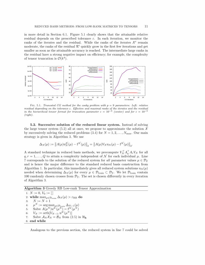
in more detail in Section 6.1. Figure 5.1 clearly shows that the attainable relativeresidual depends on the prescribed tolerance ε. In each iteration, we monitor theranks of the iterates and the residual. While the ranks of the iterates X i remainmoderate, the ranks of the residual Ri quickly grow in the first few iterations and getsmaller as soon as the attainable accuracy is reached. The intermediate large ranks inthe residual have a strong negative impact on efficiency; for example, the complexityof tensor truncation is O(k4).

1e-05

1e-04

1e-03

1e-02

1e-01

1e+00

1e+01

2 4 6 8 10 12 14

rela

tive

resi

dual

CG iterations

tol = 1e-03tol = 1e-04tol = 1e-05

10

20

30

40

50

60

70

80

2 4 6 8 10 12 14

rank

CG iterations

kmax(solution)keff(solution)

kmax(residual)keff(residual)

20

40

60

80

100

120

140

160

180

200

2 4 6 8 10 12 14

rank

CG iterations


kmax(residual)keff(residual)

Fig. 5.1. Truncated CG method for the cooky problem with p = 9 parameters: Left: relativeresidual depending on the tolerance ε. Effective and maximal ranks of the iterates and the residualin the hierarchical tensor format for truncation parameter ε = 10−3 (center) and for ε = 10−5

(right).

5.2. Successive solution of the reduced linear system. Instead of solvingthe large tensor system (5.2) all at once, we propose to approximate the solution Xby successively solving the reduced problems (3.4) for N = 1, 2, . . . , Nmax. Our mainstrategy is given in Algorithm 3. We use

∆N (µ) :=∥

∥A(µ)uNN (µ)− fN (µ)∥

∥

2=

∥

∥A(µ)VNuN (µ)− fN (µ)∥

∥

2.

A standard technique in reduced basis methods, we precompute V ⊤N A⊤

q ArVN for allq, r = 1, . . . , Q to attain a complexity independent of N for each individual µ. Line7 corresponds to the solution of the reduced system for all parameter values µ ∈ DI

and is hence the major difference to the standard reduced basis construction fromAlgorithm 1. In particular, this immediately gives all reduced system solutions uN (µ)needed when determining ∆N (µ) for every µ ∈ Dtrain ⊂ DI . We let Dtrain contain100 randomly chosen crosses from DI . The set is chosen differently in every iterationof Algorithm 3.

Algorithm 3 Greedy RB Low-rank Tensor Approximation

1: N := 0, V0 := [ ]2: while maxµ∈Dtrain

∆N (µ) > εRB do

3: N := N + 14: µN := argmaxµ∈Dtrain

∆N−1(µ)5: Solve A(µN )uN (µN ) = fN (µN )6: VN := orth[VN−1, u

N (µN )]7: Solve ANXN = BN from (2.5) in Hk

8: end while

Analogous to the previous section, the reduced system in line 7 could be solved


iteratively. To accelerate the convergence, we could again use a rank-one precondi-tioner

PN := II ⊗ PN

with PN ∈ RN×N defined by

PN :=

Q∑

q=1

λqAN,q, AN,q = V ⊤N AqVN .

Since N can be expected to remain small, the matrix PN can be explicitly inverted.However, for increasingN we can expect the same problematic rank behavior observedin Figure 5.1, because the reduced spaces XN tend to represent increasingly betterapproximations of the truth finite element space XN . Our numerical experimentsconfirm this expectation.

To circumvent the problems inherent to iterative schemes, we propose to usea completely different approach, which benefits from the reduced tensor size of thesolution. Going back to (3.3), we know that each instance µ ∈ DI of the parameterdefines a reduced solution uN (µ) = AN (µ)−1fN (µ). Since the evaluation of uN forsmall N is cheap, we can find the n1 × n2 × · · · × np × N tensor XN ∈ R

nI ·N fromthis relation directly via the cross approximation technique from [4]. Note that wecan always check the accuracy of the obtained solution a posteriori by computing theresidual RN = BN −ANXN .

6. Numerical Experiments. In this section, numerical experiments illustratethe feasibility and efficiency of the novel rbTensor algorithm summarized in Algorithm4. We study the properties of our methodology for three examples adapted from theliterature: the cooky problem from [37], a non-affine elliptic example from [15], andthe thermal fin problem from [8, 9, 36].

Algorithm 4 rbTensor

1: Obtain low-rank tensor approximations of A(µ) and fN (µ) using Algorithm 2 andtensor cross approximation

2: Approximate uN (µ) using Algorithm 3 combined with cross approximation forsolving linear systems

In all examples, we discretize the parameter domain D ⊂ Rp by a tensor grid

DI ⊂ D of 10 Chebyshev points in each parameter direction. For each dimension p,we choose the tree TD for the hierarchical tensor format Hk in the form depicted inFigure 6.1 where the leaf node p + 1 corresponds to the physical direction. Thesubtree T1,...,p is then constructed in a balanced way as in Figure 3.1 (left).

For each problem, we construct an approximation of the linear operator A byMDEIM and the approximation of Θ inHk as described in Section 4. In particular thismeans that we ignore any a priori knowledge on the affine structure of the associatedbilinear form. In the second step, we greedily construct a reduced basis approximationof the solution u. For each dimension N of the reduced basis space VN , we solve theprojected large tensor system (3.3) by a black box strategy.

To study the behavior of the reduced basis approximation, we randomly choosea test set Dtest ⊂ DI of 100 sample points for which we report the relative errors of


D = 1, 2, 3, 4, 5

1, 2, 3, 4 5

1, 2 3, 4

1 2 3 4 T1,2,3,4

Fig. 6.1. Dimension tree TD for rbTensor for p = 4.

the solution and the residual:

max err sol rel := maxµ∈Dtest

‖uN (µ)− uN (µ)‖2‖uN (µ)‖2

max err res rel := maxµ∈Dtest

‖A(µ)uN (µ)− fN (µ)‖2‖fN (µ)‖2

.

For a given output functional ℓ : X → R, we measure the relative error:

max err out rel := maxµ∈Dtest

|ℓ(uN (µ))− ℓ(uN (µ))|

|ℓ(uN (µ))|.

To analyze the properties of the low-rank tensor approximation, we determinefor each N the maximal ranks and effective ranks in the solution tensor XN and inthe output functional ℓ. For each N , we compute the non-increasing singular values

σ(N)1 , . . . , σ

(N)N of the matricization Mp+1(XN ) and report the relative singular value

σ(N)rel := σ

(N)N /σ

(N)1 (6.1)

to indicate the separation properties of XN in terms of the parameter-dependent fromthe parameter-independent part.

In each example, we measure the time tN for the assembly and solution of the fullFEM problem of size N , the time tN for the online evaluation of the reduced basisapproximation represented in the low-rank tensor format, and the online time tℓ forthe evaluation of the output functional ℓ. The timings for the full FEM solution havebeen obtained by a sparse direct solver from an average over 100 independent runsand for the reduced basis approximation by an average over 10.000 runs.

All numerical experiments have been carried out on a quad-core Intel(R) Xeon(R)CPU E31225 with 3.10GHz. Timings are CPU times for a single core. For the FEMapproximation we have used the software library deal.II [5].

6.1. Cooky Problem. Let Ω = (0, 1)2 and X = H10 (Ω). We consider the cooky

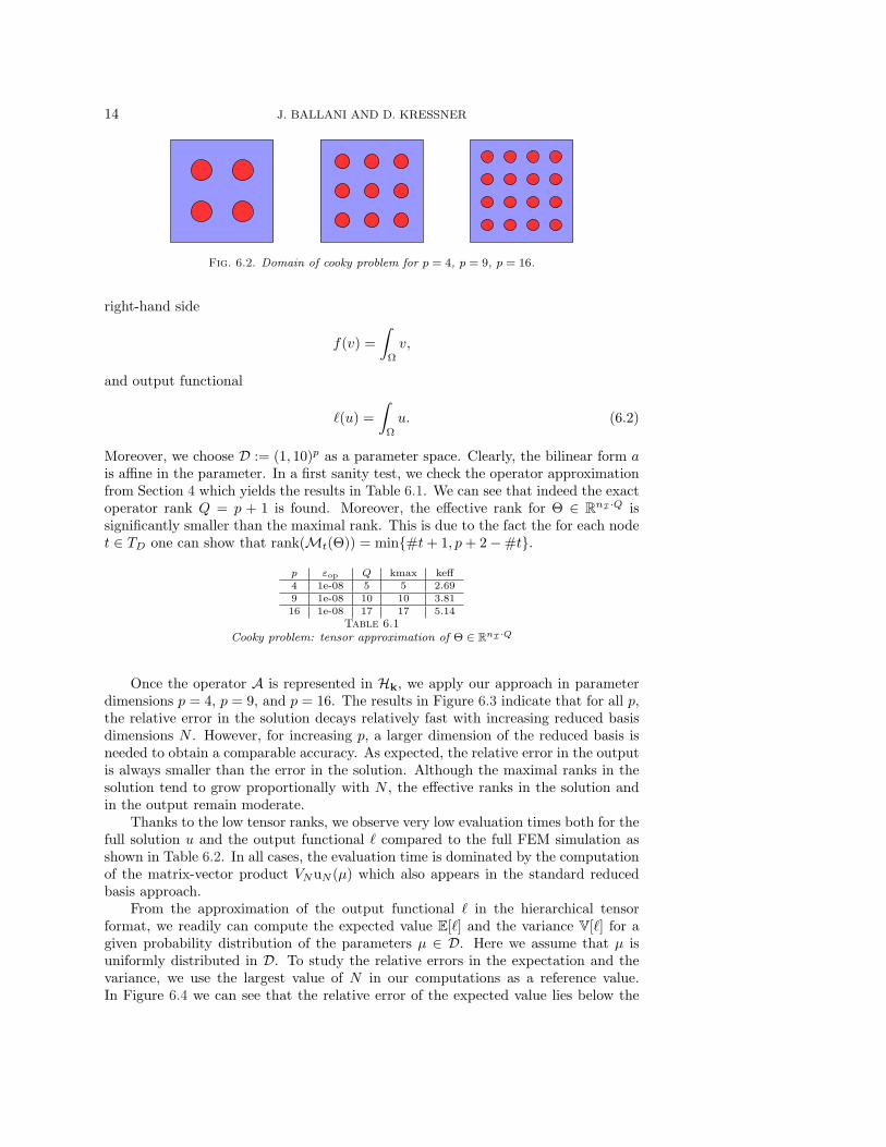
problem adapted from [37]. The domain Ω encloses disks Ω1, . . . ,Ωp of radius r whichare located at a distance of 2r from each other and from the boundary of Ω. Anillustration of this setting is shown in Figure 6.2 for p = 4 with r = 1/10, for p = 9with r = 1/14, and for p = 16 with r = 1/18.

Let now Ω0 := Ω \⋃p

i=1 Ωi. We consider the variational problem (2.1) with

a(u, v;µ) =

∫

Ω0

∇u · ∇v +

p∑

i=1

µi

∫

Ωi

∇u · ∇v,


Fig. 6.2. Domain of cooky problem for p = 4, p = 9, p = 16.

right-hand side

f(v) =

∫

Ω

v,

and output functional

ℓ(u) =

∫

Ω

u. (6.2)

Moreover, we choose D := (1, 10)p as a parameter space. Clearly, the bilinear form ais affine in the parameter. In a first sanity test, we check the operator approximationfrom Section 4 which yields the results in Table 6.1. We can see that indeed the exactoperator rank Q = p + 1 is found. Moreover, the effective rank for Θ ∈ R

nI ·Q issignificantly smaller than the maximal rank. This is due to the fact the for each nodet ∈ TD one can show that rank(Mt(Θ)) = min#t+ 1, p+ 2−#t.

p εop Q kmax keff

4 1e-08 5 5 2.69

9 1e-08 10 10 3.81

16 1e-08 17 17 5.14

Table 6.1Cooky problem: tensor approximation of Θ ∈ R

nI ·Q

Once the operator A is represented in Hk, we apply our approach in parameterdimensions p = 4, p = 9, and p = 16. The results in Figure 6.3 indicate that for all p,the relative error in the solution decays relatively fast with increasing reduced basisdimensions N . However, for increasing p, a larger dimension of the reduced basis isneeded to obtain a comparable accuracy. As expected, the relative error in the outputis always smaller than the error in the solution. Although the maximal ranks in thesolution tend to grow proportionally with N , the effective ranks in the solution andin the output remain moderate.

Thanks to the low tensor ranks, we observe very low evaluation times both for thefull solution u and the output functional ℓ compared to the full FEM simulation asshown in Table 6.2. In all cases, the evaluation time is dominated by the computationof the matrix-vector product VNuN (µ) which also appears in the standard reducedbasis approach.

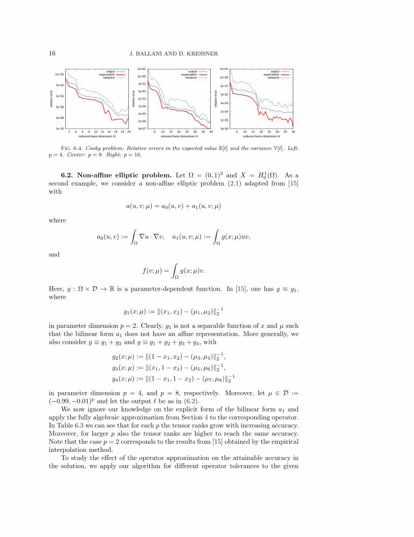
From the approximation of the output functional ℓ in the hierarchical tensorformat, we readily can compute the expected value E[ℓ] and the variance V[ℓ] for agiven probability distribution of the parameters µ ∈ D. Here we assume that µ isuniformly distributed in D. To study the relative errors in the expectation and thevariance, we use the largest value of N in our computations as a reference value.In Figure 6.4 we can see that the relative error of the expected value lies below the


1e-08

1e-07

1e-06

1e-05

1e-04

1e-03

1e-02

1e-01

1e+00

1e+01

5 10 15 20 25 30

rela

tive

erro

r

reduced basis dimension N

solutionresidual

sigma_rel

1e-08

1e-07

1e-06

1e-05

1e-04

1e-03

1e-02

1e-01

1e+00

1e+01

5 10 15 20 25 30

rela

tive

erro

rreduced basis dimension N

solutionoutput

0

5

10

15

20

25

30

5 10 15 20 25 30

rank



keff(output)

1e-06

1e-05

1e-04

1e-03

1e-02

1e-01

1e+00

1e+01

5 10 15 20 25 30 35 40 45 50

rela

tive

erro

r


solutionresidual

sigma_rel

1e-08

1e-07

1e-06

1e-05

1e-04

1e-03

1e-02

1e-01

1e+00

1e+01

5 10 15 20 25 30 35 40 45 50

rela

tive

erro

r


solutionoutput

0

10

20

30

40

50

60

70

80

90

5 10 15 20 25 30 35 40 45 50

rank



keff(output)

1e-05

1e-04

1e-03

1e-02

1e-01

1e+00

1e+01

5 10 15 20 25 30 35 40 45 50

rela

tive

erro

r


solutionresidual

sigma_rel

1e-05

1e-04

1e-03

1e-02

1e-01

1e+00

1e+01

5 10 15 20 25 30 35 40 45 50

rela

tive

erro

r


solutionoutput

0

5

10

15

20

25

30

35

40

45

50

5 10 15 20 25 30 35 40 45 50

rank



keff(output)

Fig. 6.3. Cooky problem: Top: p = 4. Center: p = 9. Bottom: p = 16. Left: error in the

solution and in the residual and σ(N)rel from (6.1). Center: error in the output functional. Right:

tensor ranks for the solution and the output.

p N tN [s] N tN [s] tℓ [s] tN /tN tN /tℓ tmatvec [s]

4 1169 1.0e-02 10 6.8e-06 1.7e-06 1488 5857 6.3e-0620 1.6e-05 7.0e-06 630 1437 9.4e-0630 2.7e-05 1.2e-05 374 824 1.5e-05

9 2796 2.6e-02 10 1.5e-05 2.2e-06 1797 11816 1.4e-0520 4.6e-05 2.4e-05 568 1093 2.3e-0530 9.7e-05 6.3e-05 271 416 3.6e-0540 1.2e-04 7.8e-05 216 336 4.5e-0550 2.5e-04 2.0e-04 104 130 5.8e-05


Table 6.2Cooky problem: evaluation times tN for full FEM solution, tN for online evaluation of uN ,

tℓ for online evaluation of ℓ compared to tmatvec for computing the product VNuN (µ) for a singleparameter tuple µ

relative error of the output ℓ whereas the error variance typically lies one or two ordersabove this error.


1e-10

1e-08

1e-06

1e-04

1e-02

1e+00

2 4 6 8 10 12 14 16 18 20

rela

tive

erro

r


outputexpectation

variance

1e-07

1e-06

1e-05

1e-04

1e-03

1e-02

1e-01

1e+00

1e+01

5 10 15 20 25 30 35 40re

lativ

e er

ror


outputexpectation

variance

1e-06

1e-05

1e-04

1e-03

1e-02

1e-01

1e+00

1e+01

5 10 15 20 25 30 35 40

rela

tive

erro

r


outputexpectation

variance

Fig. 6.4. Cooky problem: Relative errors in the expected value E[ℓ] and the variance V[ℓ]. Left:p = 4. Center: p = 9. Right: p = 16.

6.2. Non-affine elliptic problem. Let Ω = (0, 1)2 and X = H10 (Ω). As a

second example, we consider a non-affine elliptic problem (2.1) adapted from [15]with

a(u, v;µ) = a0(u, v) + a1(u, v;µ)

where

a0(u, v) :=

∫

Ω

∇u · ∇v, a1(u, v;µ) :=

∫

Ω

g(x;µ)uv,

and

f(v;µ) =

∫

Ω

g(x;µ)v.

Here, g : Ω × D → R is a parameter-dependent function. In [15], one has g ≡ g1,where

g1(x;µ) := ‖(x1, x2)− (µ1, µ2)‖−12

in parameter dimension p = 2. Clearly, g1 is not a separable function of x and µ suchthat the bilinear form a1 does not have an affine representation. More generally, wealso consider g ≡ g1 + g2 and g ≡ g1 + g2 + g3 + g4, with

g2(x;µ) := ‖(1− x1, x2)− (µ3, µ4)‖−12 ,

g3(x;µ) := ‖(x1, 1− x2)− (µ5, µ6)‖−12 ,

g4(x;µ) := ‖(1− x1, 1− x2)− (µ7, µ8)‖−12

in parameter dimension p = 4, and p = 8, respectively. Moreover, let µ ∈ D :=(−0.99,−0.01)p and let the output ℓ be as in (6.2).

We now ignore our knowledge on the explicit form of the bilinear form a1 andapply the fully algebraic approximation from Section 4 to the corresponding operator.In Table 6.3 we can see that for each p the tensor ranks grow with increasing accuracy.Moreover, for larger p also the tensor ranks are higher to reach the same accuracy.Note that the case p = 2 corresponds to the results from [15] obtained by the empiricalinterpolation method.

To study the effect of the operator approximation on the attainable accuracy inthe solution, we apply our algorithm for different operator tolerances to the given


p = 2 p = 4 p = 8

εop Q kmax keff Q kmax keff Q kmax keff

1e-03 10 10 5.78 15 15 7.44 21 21 8.761e-04 14 14 7.36 23 23 11.33 35 35 14.451e-05 20 20 9.83 34 34 15.76 49 49 19.841e-06 25 25 10.88 44 44 19.81 66 66 26.50

Table 6.3Non-affine problem: tensor approximation of Θ ∈ R

nI ·Q.

1e-07

1e-06

1e-05

1e-04

1e-03

1e-02

1e-01

1e+00

5 10 15 20 25

rela

tive

solu

tion

erro

r


tol_op = 1e-3tol_op = 1e-4tol_op = 1e-5tol_op = 1e-6

1e-07

1e-06

1e-05

1e-04

1e-03

1e-02

1e-01

1e+00

5 10 15 20 25 30 35 40 45

rela

tive

solu

tion

erro

r



1e-07

1e-06

1e-05

1e-04

1e-03

1e-02

1e-01

1e+00

5 10 15 20 25 30 35 40 45 50

rela

tive

solu

tion

erro

r



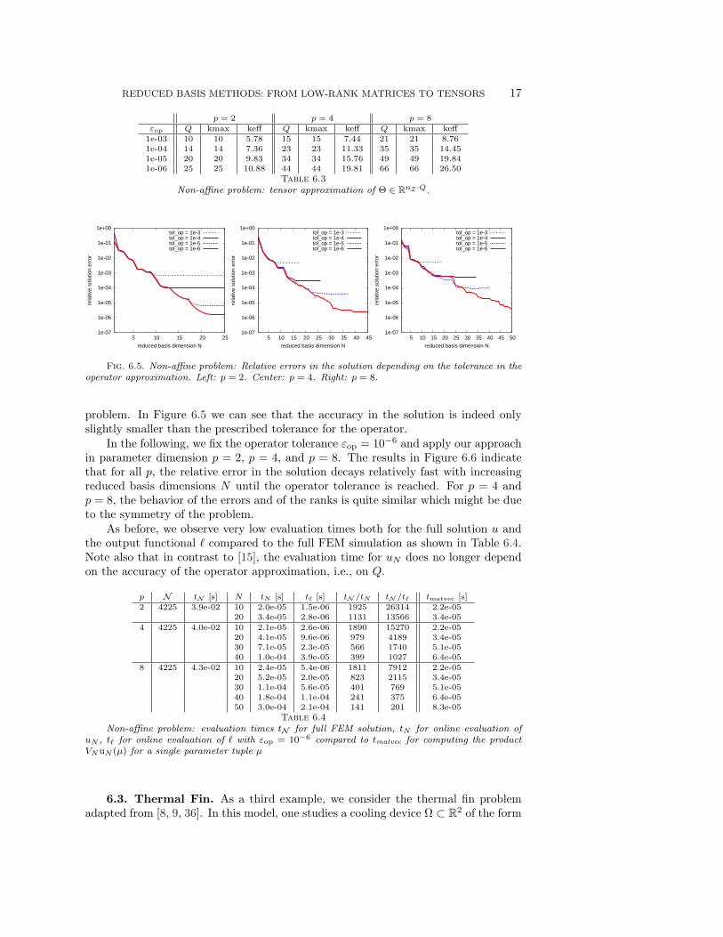
Fig. 6.5. Non-affine problem: Relative errors in the solution depending on the tolerance in theoperator approximation. Left: p = 2. Center: p = 4. Right: p = 8.

problem. In Figure 6.5 we can see that the accuracy in the solution is indeed onlyslightly smaller than the prescribed tolerance for the operator.

In the following, we fix the operator tolerance εop = 10−6 and apply our approachin parameter dimension p = 2, p = 4, and p = 8. The results in Figure 6.6 indicatethat for all p, the relative error in the solution decays relatively fast with increasingreduced basis dimensions N until the operator tolerance is reached. For p = 4 andp = 8, the behavior of the errors and of the ranks is quite similar which might be dueto the symmetry of the problem.

As before, we observe very low evaluation times both for the full solution u andthe output functional ℓ compared to the full FEM simulation as shown in Table 6.4.Note also that in contrast to [15], the evaluation time for uN does no longer dependon the accuracy of the operator approximation, i.e., on Q.


2 4225 3.9e-02 10 2.0e-05 1.5e-06 1925 26314 2.2e-0520 3.4e-05 2.8e-06 1131 13566 3.4e-05

4 4225 4.0e-02 10 2.1e-05 2.6e-06 1890 15270 2.2e-0520 4.1e-05 9.6e-06 979 4189 3.4e-0530 7.1e-05 2.3e-05 566 1740 5.1e-0540 1.0e-04 3.9e-05 399 1027 6.4e-05


Table 6.4Non-affine problem: evaluation times tN for full FEM solution, tN for online evaluation of

uN , tℓ for online evaluation of ℓ with εop = 10−6 compared to tmatvec for computing the productVNuN (µ) for a single parameter tuple µ

6.3. Thermal Fin. As a third example, we consider the thermal fin problemadapted from [8, 9, 36]. In this model, one studies a cooling device Ω ⊂ R

2 of the form


1e-07

1e-06

1e-05

1e-04

1e-03

1e-02

1e-01

1e+00

5 10 15 20 25

rela

tive

erro

r


solutionresidual

sigma_rel

1e-07

1e-06

1e-05

1e-04

1e-03

1e-02

1e-01

1e+00

5 10 15 20 25

rela

tive

erro

rreduced basis dimension N

solutionoutput

0

5

10

15

20

25

5 10 15 20 25

rank



keff(output)

1e-07

1e-06

1e-05

1e-04

1e-03

1e-02

1e-01

1e+00

5 10 15 20 25 30 35 40 45

rela

tive

erro

r


solutionresidual

sigma_rel

1e-07

1e-06

1e-05

1e-04

1e-03

1e-02

1e-01

1e+00

5 10 15 20 25 30 35 40 45 50

rela

tive

erro

r


solutionoutput

0

5

10

15

20

25

30

35

40

45

5 10 15 20 25 30 35 40 45

rank



keff(output)

1e-07

1e-06

1e-05

1e-04

1e-03

1e-02

1e-01

1e+00

5 10 15 20 25 30 35 40 45 50

rela

tive

erro

r


solutionresidual

sigma_rel

1e-07

1e-06

1e-05

1e-04

1e-03

1e-02

1e-01

1e+00

5 10 15 20 25 30 35 40 45 50

rela

tive

erro

r


solutionoutput

0

5

10

15

20

25

30

35

40

45

50

5 10 15 20 25 30 35 40 45 50

rank



keff(output)

Fig. 6.6. Non-affine problem: Top: p = 2. Center: p = 4. Bottom: p = 8. Left: error in the



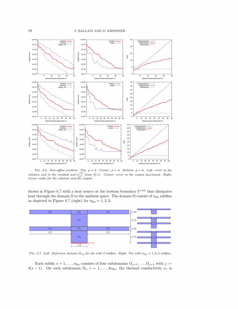
shown in Figure 6.7 with a heat source at the bottom boundary Γroot that dissipatesheat through the domain Ω to the ambient space. The domain Ω consist of nfin subfinsas depicted in Figure 6.7 (right) for nfin = 1, 2, 3.

Ω1Ω2

Ω3

Ω4

Ω5Ω6

Ω7

Ω8

1.0

2.52.5

0.75

0.25

0.75

0.25

Γroot

Fig. 6.7. Left: Reference domain Ωref for fin with 2 subfins. Right: Fin with nfin = 1, 2, 3 subfins

Each subfin s = 1, . . . , nfin consists of four subdomains Ωj+1, . . . ,Ωj+4 with j :=4(s − 1). On each subdomain Ωi, i = 1, . . . , 4nfin, the thermal conductivity κi is


assumed to be constant. The steady-state temperature distribution u is given by

−κi∆u = 0 in Ωi, i = 1, . . . 4nfin.

At the interior boundaries Γinti,j := ∂Ωi∩∂Ωj , i 6= j, we impose the interface conditions

u|Ωi= u|Ωj

on Γinti,j ,

−κi(∂u/∂ni) = −κj(∂u/∂nj) on Γinti,j ,

where ni, nj are the outer normals of Ωi,Ωj , respectively. On the exterior boundariesΓexti := ∂Ωi\

⋃

j Γinti,j , we model the convective heat loss by Robin boundary conditions

of the form

−κi(∂u/∂ni) = Biu on Γexti

where Bi is the Biot number. Finally, we impose a heat source at the bottom boundaryΓroot by the Neumann condition

−κ3(∂u/∂n3) = −1 on Γroot.

The variational formulation of this problem is then given by (2.1) with X = H1(Ω)and

a(u, v) :=

4nfin∑

i=1

κi

∫

Ωi

∇u · ∇v + Bi

4nfin∑

i=1

∫

Γexti

uv

and

f(v) :=

∫

Γroot

v.

We now parametrize this model by a parameter vector µ ∈ D ⊂ Rp with p := 4nfin+3

in the following way:1. For each subfin s = 1, . . . , nfin, we parametrize the heat conductivity of the

domains Ωj+1 and Ωj+2, j := 4(s − 1), by setting κj+1 = κj+2 := µj+1.For the rest of the subdomains, we assume an identical conductivity κj+3 =κj+4 := µ4nfin+1.The range of the parameters is given by µj+1, µ4nfin+1 ∈ [0.5, 2.0].

2. For each subfin s = 1, . . . , nfin, we parametrize the shape of the domains Ωj+1

and Ωj+2, j := 4(s−1), to be rectangles of size 2.5µj+2×0.25µj+3. Moreover,Ωj+3 is assumed to be a rectangle of size µ4nfin+2 × 0.75µj+4 which makesΩj+4 a rectangle of size µ4nfin+2 × 0.25µj+3.The range of the parameters is given by µj+2, µj+3, µ4nfin+2 ∈ [0.8, 1.2].

3. We set the Biot number to Bi := µ4nfin+3.The range of the parameter is given by µ4nfin+3 ∈ [0.5, 2].

Thanks to the Cartesian product structure of the domain, the parametrized problemcan be easily transformed to a variational problem on a reference domain Ωref depictedin Figure 6.7 (left) for the case nfin = 2. For the details we refer to [8]. As an outputfunctional, we again choose ℓ from (6.2).

It can be shown that the linear operator associated to the bilinear form a onthe reference domain again allows for an affine representation. This structure isautomatically found by our algorithm, cf. Table 6.5.


p εop Q kmax keff

7 1e-08 10 10 4.95

11 1e-08 19 19 6.93

15 1e-08 28 28 8.52

Table 6.5Thermal fin: tensor approximation of Θ ∈ R

nI ·Q

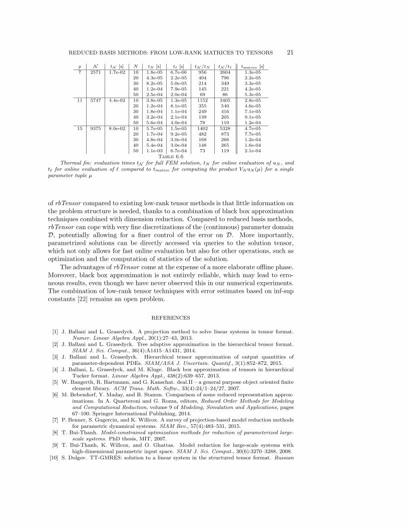
The results in Figure 6.8 illustrate that the dimensionN of the reduced basis needsto be chosen significantly larger to reach the same accuracy when the complexity ofthe problem is increased (larger nfin). For a fixed dimension N , the tensor ranks ofthe solution grow only mildly with increasing nfin. Note however that for a fixedaccuracy, also the required tensor ranks are higher. The computational savings intime shown in Table 6.6 show a similar behavior as in the previous examples.

1e-05

1e-04

1e-03

1e-02

1e-01

1e+00

5 10 15 20 25 30 35 40 45 50

rela

tive

erro

r


solutionresidual

sigma_rel

1e-05

1e-04

1e-03

1e-02

1e-01

1e+00

5 10 15 20 25 30 35 40 45 50

rela

tive

erro

r


solutionoutput

0

10

20

30

40

50

60

70

80

5 10 15 20 25 30 35 40 45 50

rank



keff(output)

1e-05

1e-04

1e-03

1e-02

1e-01

1e+00

5 10 15 20 25 30 35 40 45 50

rela

tive

erro

r


solutionresidual

sigma_rel

1e-05

1e-04

1e-03

1e-02

1e-01

1e+00

5 10 15 20 25 30 35 40 45 50

rela

tive

erro

r


solutionoutput

0

20

40

60

80

100

120

5 10 15 20 25 30 35 40 45 50

rank



keff(output)

1e-05

1e-04

1e-03

1e-02

1e-01

1e+00

5 10 15 20 25 30 35 40 45 50

rela

tive

erro

r


solutionresidual

sigma_rel

1e-05

1e-04

1e-03

1e-02

1e-01

1e+00

5 10 15 20 25 30 35 40 45 50

rela

tive

erro

r


solutionoutput

0

20

40

60

80

100

120

5 10 15 20 25 30 35 40 45 50

rank



keff(output)

Fig. 6.8. Thermal fin: Top: p = 7. Center: p = 11. Bottom: p = 15. Left: error in the



7. Conclusions. We have proposed a new method, called rbTensor, for theefficient solution of parametrized linear systems. Combining techniques from reducedbasis methods and low-rank tensor approximation, our method is particularly suitedin the presence of many parameters and nonlinear dependencies. A major advantage






Table 6.6Thermal fin: evaluation times tN for full FEM solution, tN for online evaluation of uN , and

tℓ for online evaluation of ℓ compared to tmatvec for computing the product VNuN (µ) for a singleparameter tuple µ

of rbTensor compared to existing low-rank tensor methods is that little information onthe problem structure is needed, thanks to a combination of black box approximationtechniques combined with dimension reduction. Compared to reduced basis methods,rbTensor can cope with very fine discretizations of the (continuous) parameter domainD, potentially allowing for a finer control of the error on D. More importantly,parametrized solutions can be directly accessed via queries to the solution tensor,which not only allows for fast online evaluation but also for other operations, such asoptimization and the computation of statistics of the solution.

The advantages of rbTensor come at the expense of a more elaborate offline phase.Moreover, black box approximation is not entirely reliable, which may lead to erro-neous results, even though we have never observed this in our numerical experiments.The combination of low-rank tensor techniques with error estimates based on inf-supconstants [22] remains an open problem.

REFERENCES

[1] J. Ballani and L. Grasedyck. A projection method to solve linear systems in tensor format.Numer. Linear Algebra Appl., 20(1):27–43, 2013.

[2] J. Ballani and L. Grasedyck. Tree adaptive approximation in the hierarchical tensor format.SIAM J. Sci. Comput., 36(4):A1415–A1431, 2014.

[3] J. Ballani and L. Grasedyck. Hierarchical tensor approximation of output quantities ofparameter-dependent PDEs. SIAM/ASA J. Uncertain. Quantif., 3(1):852–872, 2015.

[4] J. Ballani, L. Grasedyck, and M. Kluge. Black box approximation of tensors in hierarchicalTucker format. Linear Algebra Appl., 438(2):639–657, 2013.

[5] W. Bangerth, R. Hartmann, and G. Kanschat. deal.II – a general purpose object oriented finiteelement library. ACM Trans. Math. Softw., 33(4):24/1–24/27, 2007.

[6] M. Bebendorf, Y. Maday, and B. Stamm. Comparison of some reduced representation approx-imations. In A. Quarteroni and G. Rozza, editors, Reduced Order Methods for Modelingand Computational Reduction, volume 9 of Modeling, Simulation and Applications, pages67–100. Springer International Publishing, 2014.

[7] P. Benner, S. Gugercin, and K. Willcox. A survey of projection-based model reduction methodsfor parametric dynamical systems. SIAM Rev., 57(4):483–531, 2015.

[8] T. Bui-Thanh. Model-constrained optimization methods for reduction of parameterized large-scale systems. PhD thesis, MIT, 2007.

[9] T. Bui-Thanh, K. Willcox, and O. Ghattas. Model reduction for large-scale systems withhigh-dimensional parametric input space. SIAM J. Sci. Comput., 30(6):3270–3288, 2008.

[10] S. Dolgov. TT-GMRES: solution to a linear system in the structured tensor format. Russian


J. Numer. Anal. Math. Modelling, 28(2):149–172, 2013.[11] S. Dolgov and I. V. Oseledets. Solution of linear systems and matrix inversion in the TT-format.

SIAM J. Sci. Comput., 34(5):A2718–A2739, 2012.[12] S. Dolgov and D. V. Savostyanov. Alternating minimal energy methods for linear systems in

higher dimensions. SIAM J. Sci. Comput., 36(5):A2248–A2271, 2014.[13] L. Grasedyck. Hierarchical singular value decomposition of tensors. SIAM J. Matrix Anal.

Appl., 31:2029–2054, 2010.[14] L. Grasedyck, D. Kressner, and C. Tobler. A literature survey of low-rank tensor approximation

techniques. GAMM-Mitteilungen, 36(1):53–78, 2013.[15] M. A. Grepl, Y. Maday, N. C. Nguyen, and A. T. Patera. Efficient reduced-basis treatment

of nonaffine and nonlinear partial differential equations. ESAIM, Math. Model. Numer.Anal., 41(3):575–605, 2007.

[16] W. Hackbusch. Tensor Spaces and Numerical Tensor Calculus. Springer, Berlin, 2012.[17] W. Hackbusch and S. Kuhn. A new scheme for the tensor representation. J. Fourier Anal.

Appl., 15(5):706–722, 2009.[18] J. S. Hesthaven, G. Rozza, and B. Stamm. Certified Reduced Basis Methods for Parametrized

Partial Differential Equations. Springer, Berlin, 2016.[19] J. S. Hesthaven, B. Stamm, and S. Zhang. Efficient greedy algorithms for high-dimensional

parameter spaces with applications to empirical interpolation and reduced basis methods.ESAIM: Mathematical Modelling and Numerical Analysis, 48(1):259–283, 2014.

[20] N. J. Higham. Accuracy and Stability of Numerical Algorithms. SIAM, Philadelphia, PA,second edition, 2002.

[21] S. Holtz, T. Rohwedder, and R. Schneider. The alternating linear scheme for tensor optimizationin the tensor train format. SIAM J. Sci. Comput., 34(2):A683–A713, 2012.

[22] D. B. P. Huynh, D. J. Knezevic, Y. Chen, J. S. Hesthaven, and A. T. Patera. A natural-normsuccessive constraint method for inf-sup lower bounds. Comput. Methods Appl. Mech.Engrg., 199(29-32):1963–1975, 2010.

[23] B. N. Khoromskij and I. Oseledets. Quantics-TT collocation approximation of parameter-dependent and stochastic elliptic PDEs. Comp. Meth. in Applied Math., 10(4):376–394,2010.

[24] B. N. Khoromskij and C. Schwab. Tensor-structured Galerkin approximation of parametricand stochastic elliptic PDEs. SIAM J. Sci. Comput., 33(1):364–385, 2011.

[25] T. G. Kolda and B. W. Bader. Tensor decompositions and applications. SIAM Review,51(3):455–500, 2009.

[26] D. Kressner, M. Plesinger, and C. Tobler. A preconditioned low-rank CG method for parameter-dependent Lyapunov matrix equations. Numer. Linear Algebra Appl., 21(5):666–684, 2014.

[27] D. Kressner, M. Steinlechner, and B. Vandereycken. Preconditioned low-rank Riemannianoptimization for linear systems with tensor product structure. Preprint, EPFL-SB-MATHICSE-ANCHP, 2015.

[28] D. Kressner and C. Tobler. Low-rank tensor Krylov subspace methods for parameterized linearsystems. SIAM J. Matrix Anal. Appl., 32(4):1288–1316, 2011.

[29] H. G. Matthies and E. Zander. Solving stochastic systems with low-rank tensor compression.Linear Algebra Appl., 436(10):3819–3838, 2012.

[30] G. Migliorati, F. Nobile, E. von Schwerin, and R. Tempone. Approximation of quantities ofinterest in stochastic PDEs by the random discrete L2 projection on polynomial spaces.SIAM J. Sci. Comput., 35(3):A1440–A1446, 2013.

[31] F. Negri, A. Manzoni, and D. Amsallem. Efficient model reduction of parametrized systems bymatrix discrete empirical interpolation. J. Comput. Phys., 303:431–454, 2015.

[32] I. V. Oseledets. DMRG approach to fast linear algebra in the TT-format. Comput. Meth. Appl.Math, 11(3):382–393, 2011.

[33] I. V. Oseledets. Tensor-train decomposition. SIAM J. Sci. Comput., 33(5):2295–2317, 2011.[34] A. Quarteroni, A. Manzoni, and F. Negri. Reduced Basis Methods for Partial Differential

Equations. Springer, Unitext Series, vol. 92, 2016.[35] G. Rozza, D. B. P. Huynh, and A. T. Patera. Reduced basis approximation and a posteriori

error estimation for affinely parametrized elliptic coercive partial differential equations.Arch. Comput. Methods Eng., 15:229–275, 2008.

[36] Y. O. Solodukhov. Reduced-basis methods applied to locally non-affine and locally non-linearpartial differential equations. PhD thesis, MIT, 2005.

[37] C. Tobler. Low-rank Tensor Methods for Linear Systems and Eigenvalue Problems. PhD thesis,ETH Zurich, 2012.

reduced basis methods: from low-rank matrices to...

Documents