Prepared by:

Adam BoiesDavid KittelsonWinthrop WattsDepartment of Mechanical Engineering

Jan LuckeLaurie McGinnisCenter for Transportation Studies

Julian MarshallTyler PattersonDepartment of Civil Engineering

Peter NussbaumElizabeth WilsonHumphrey Institute of Public Affairs

University of Minnesota

Reducing Greenhouse Gas Emissions From Transportation Sources in Minnesota

Published by:

Center for Transportation StudiesUniversity of Minnesota511 Washington Avenue S.E.Minneapolis, MN 55455

CTS 08-10

June 2008

Technical Report Documentation Page 1. Report No. 2. 3. Recipients Accession No. CTS 08-10 4. Title and Subtitle 5. Report Date

June 2008 6.

Reducing Greenhouse Gas Emissions From Transportation Sources in Minnesota

7. Author(s) 8. Performing Organization Report No. Adam Boies, David Kittelson, Winthrop Watts, Jan Lucke, Laurie McGinnis, Julian Marshall, Tyler Patterson, Peter Nussbaum, Elizabeth Wilson

9. Performing Organization Name and Address 10. Project/Task/Work Unit No. 11. Contract (C) or Grant (G) No.

12. Sponsoring Organization Name and Address 13. Type of Report and Period Covered Final Report 14. Sponsoring Agency Code

Center for Transportation Studies University of Minnesota 200 Transportation and Safety Building 511 Washington Ave. SE Minneapolis, MN 55455

15. Supplementary Notes http://www.cts.umn.edu/Publications/ResearchReports/ 16. Abstract (Limit: 250 words) The 2007 Minnesota Next Generation Energy Act established goals for reducing statewide greenhouse gas (GHG) emissions by 15% by 2015, 30% by 2025, and 80% by 2050, relative to 2005 levels. This report investigates strategies for meeting those reductions in Minnesota’s transportation sector, which produces approximately 24% of total state GHG emissions. The study focuses on three types of emission-reduction strategies: those that improve vehicle fuel economy, those that reduce the number of vehicle-miles traveled, and others that decrease the carbon content of fuel. The researchers used a quantitative model to test the effectiveness of specific strategies for GHG emission reduction from transportation in Minnesota. Modeled scenario outcomes depend strongly on input assumptions, and lead us to the following three main conclusions. 1. Meeting state goals will require all three types of policies. For example, Minnesota could adopt a GHG emissions standard, a low-carbon fuel standard, and comprehensive transit and Smart Growth policies. 2. Technologies are available today to substantially improve fuel economy and vehicle GHG emissions. Requiring these technologies could save Minnesota consumers money and better insulate them from oil price volatility. 3. Changes in vehicle-miles traveled (VMT) have a strong impact on whether the goals can be met, and increases in VMT can offset GHG reductions. Overall, the research indicates that the goals can be met, but achieving them requires consistent and concerted action beginning immediately. 17. Document Analysis/Descriptors 18. Availability Statement Greenhouse gases Air pollution Air quality management

Minnesota Exhaust gases

No restrictions. Document available from: National Technical Information Services, Springfield, Virginia 22161

19. Security Class (this report) 20. Security Class (this page) 21. No. of Pages 22. Price Unclassified Unclassified 60

Reducing Greenhouse Gas Emissions From Transportation Sources in Minnesota

Final Report

Prepared by:

Adam Boies David Kittelson Winthrop Watts

Department of Mechanical Engineering

Jan Lucke Laurie McGinnis

Center for Transportation Studies

Julian Marshall Tyler Patterson

Department of Civil Engineering

Peter Nussbaum Elizabeth Wilson

Hubert H. Humphrey Institute of Public Affairs

University of Minnesota

June 2008

Published by:

Center for Transportation Studies

University of Minnesota 511 Washington Avenue S.E.

Minneapolis, MN 55455

CTS 08-10

This report represents the results of research conducted by the authors and does not necessarily represent the views or policies of the Center for Transportation Studies. This report does not contain a standard or specified technique.

Acknowledgments This study was funded by an appropriation from the Minnesota legislature. We thank

Representatives Melissa Hortman and Frank Hornstein for their support and encouragement, and an expert review panel assembled by the Center for Transportation Studies for their extensive and helpful comments.

For more information Laurie McGinnis Associate Director Center for Transportation Studies University of Minnesota 612-625-3019 mcgin001@cts.umn.edu

TABLE OF CONTENTS

CHAPTER 1: INTRODUCTION.......................................................................................... 1

Federal Regulations and State Policies ................................................................................. 2 Trends Affecting Minnesota’s Transportation GHG Emissions........................................... 2

CHAPTER 2: ANALYTICAL APPROACH ....................................................................... 5 CHAPTER 3: INDIVIDUAL STRATEGIES ...................................................................... 7

Light-Duty Vehicle Strategies .............................................................................................. 7 Emissions and Mileage Standards .................................................................................... 7 Feebates........................................................................................................................... 11

Heavy-Duty Vehicle Strategies........................................................................................... 13 Fuel Strategies..................................................................................................................... 14

Federal Policies............................................................................................................... 15Minnesota Options .......................................................................................................... 16

Land Use and System Shift Strategies ................................................................................ 19 Techniques ...................................................................................................................... 20 Implementation Challenges ............................................................................................ 21 Transit and Smart Growth............................................................................................... 22 Options for the Twin Cities............................................................................................. 24

Other Strategies................................................................................................................... 27 CHAPTER 4: COMBINED STRATEGIES TO MEET THE 2015 AND 2025 GOALS................................................................................................................ 29

Parameters....................................................................................................................... 29 Projections for Minnesota ............................................................................................... 29 Sensitivity/Uncertainty Analysis .................................................................................... 30

CHAPTER 5: PROMISING TECHNOLOGIES AND STRATEGIES FOR ACHIEVING 2050 GOALS............................................................. 33

Hybrid Vehicles .............................................................................................................. 33 Infrastructure................................................................................................................... 34 Fuels................................................................................................................................ 34 Land Use and System Shifts ........................................................................................... 34

CHAPTER 6: CONCLUSIONS .......................................................................................... 37 REFERENCES...................................................................................................................... 39 Visit www.cts.umn.edu/Research/GreenhousGas for an electronic copy of this report and for supplemental material.

LIST OF TABLES

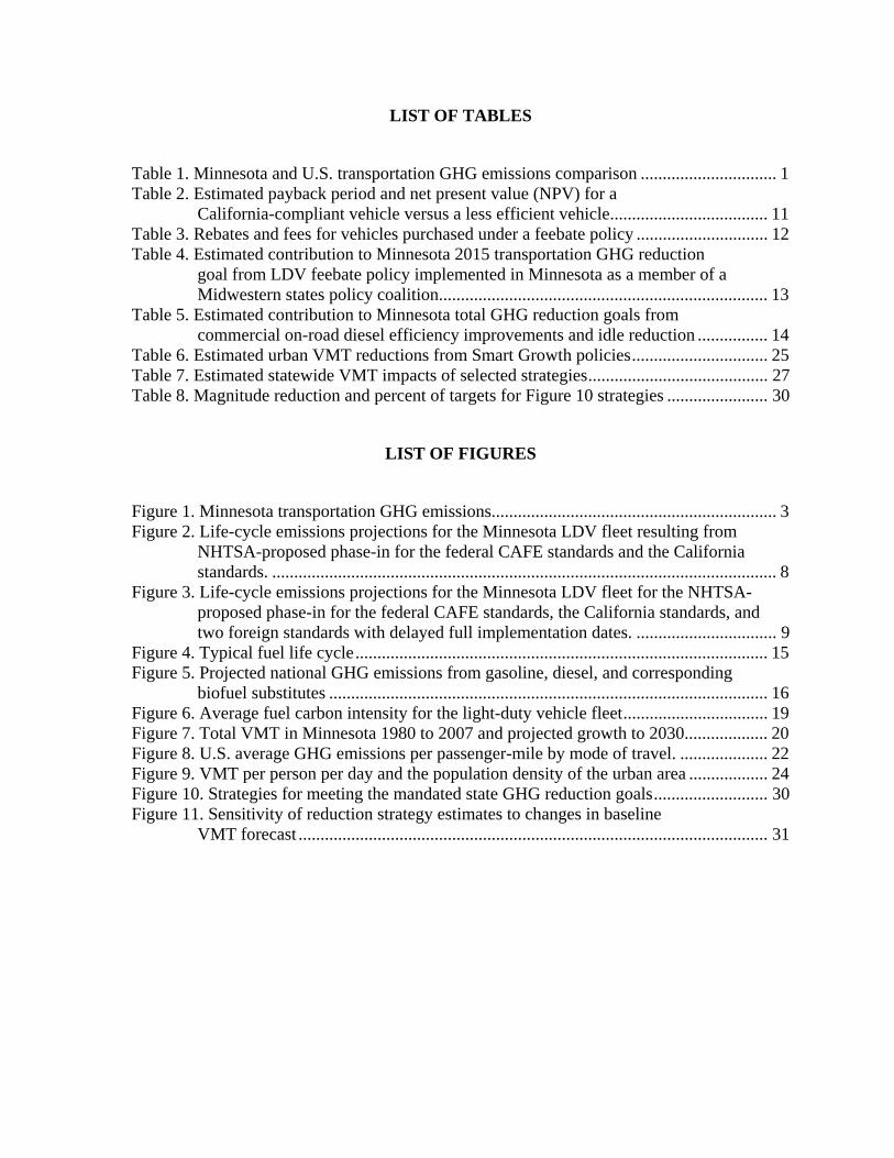
Table 1. Minnesota and U.S. transportation GHG emissions comparison ............................... 1 Table 2. Estimated payback period and net present value (NPV) for a

California-compliant vehicle versus a less efficient vehicle.................................... 11 Table 3. Rebates and fees for vehicles purchased under a feebate policy .............................. 12 Table 4. Estimated contribution to Minnesota 2015 transportation GHG reduction

goal from LDV feebate policy implemented in Minnesota as a member of a Midwestern states policy coalition........................................................................... 13

Table 5. Estimated contribution to Minnesota total GHG reduction goals from commercial on-road diesel efficiency improvements and idle reduction ................ 14

Table 6. Estimated urban VMT reductions from Smart Growth policies............................... 25 Table 7. Estimated statewide VMT impacts of selected strategies......................................... 27Table 8. Magnitude reduction and percent of targets for Figure 10 strategies ....................... 30

LIST OF FIGURES

Figure 1. Minnesota transportation GHG emissions................................................................. 3 Figure 2. Life-cycle emissions projections for the Minnesota LDV fleet resulting from

NHTSA-proposed phase-in for the federal CAFE standards and the California standards. ................................................................................................................... 8

Figure 3. Life-cycle emissions projections for the Minnesota LDV fleet for the NHTSA-proposed phase-in for the federal CAFE standards, the California standards, and two foreign standards with delayed full implementation dates. ................................ 9

Figure 4. Typical fuel life cycle.............................................................................................. 15 Figure 5. Projected national GHG emissions from gasoline, diesel, and corresponding

biofuel substitutes .................................................................................................... 16 Figure 6. Average fuel carbon intensity for the light-duty vehicle fleet................................. 19 Figure 7. Total VMT in Minnesota 1980 to 2007 and projected growth to 2030................... 20 Figure 8. U.S. average GHG emissions per passenger-mile by mode of travel. .................... 22 Figure 9. VMT per person per day and the population density of the urban area .................. 24 Figure 10. Strategies for meeting the mandated state GHG reduction goals.......................... 30 Figure 11. Sensitivity of reduction strategy estimates to changes in baseline

VMT forecast ........................................................................................................... 31

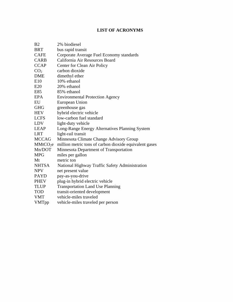
LIST OF ACRONYMS

B2 2% biodiesel BRT bus rapid transit CAFE Corporate Average Fuel Economy standards CARB California Air Resources Board CCAP Center for Clean Air Policy CO2 carbon dioxide DME dimethyl ether E10 10% ethanol E20 20% ethanol E85 85% ethanol EPA Environmental Protection Agency EU European Union GHG greenhouse gas HEV hybrid electric vehicle LCFS low-carbon fuel standard LDV light-duty vehicle LEAP Long-Range Energy Alternatives Planning System LRT light-rail transit MCCAG Minnesota Climate Change Advisory Group MMtCO2e million metric tons of carbon dioxide equivalent gases Mn/DOT Minnesota Department of Transportation MPG miles per gallon Mt metric ton NHTSA National Highway Traffic Safety Administration NPV net present value PAYD pay-as-you-drive PHEV plug-in hybrid electric vehicle TLUP Transportation Land Use Planning TOD transit-oriented development VMT vehicle-miles traveled VMTpp vehicle-miles traveled per person

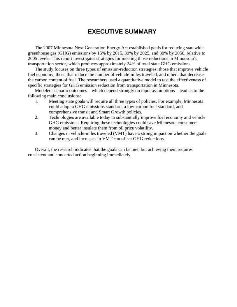
EXECUTIVE SUMMARY The 2007 Minnesota Next Generation Energy Act established goals for reducing statewide

greenhouse gas (GHG) emissions by 15% by 2015, 30% by 2025, and 80% by 2050, relative to 2005 levels. This report investigates strategies for meeting those reductions in Minnesota’s transportation sector, which produces approximately 24% of total state GHG emissions.

The study focuses on three types of emission-reduction strategies: those that improve vehicle fuel economy, those that reduce the number of vehicle-miles traveled, and others that decrease the carbon content of fuel. The researchers used a quantitative model to test the effectiveness of specific strategies for GHG emission reduction from transportation in Minnesota.

Modeled scenario outcomes—which depend strongly on input assumptions—lead us to the following main conclusions:

1. Meeting state goals will require all three types of policies. For example, Minnesota could adopt a GHG emissions standard, a low-carbon fuel standard, and comprehensive transit and Smart Growth policies.

2. Technologies are available today to substantially improve fuel economy and vehicle GHG emissions. Requiring these technologies could save Minnesota consumers money and better insulate them from oil price volatility.

3. Changes in vehicle-miles traveled (VMT) have a strong impact on whether the goals can be met, and increases in VMT can offset GHG reductions.

Overall, the research indicates that the goals can be met, but achieving them requires

consistent and concerted action beginning immediately.

1

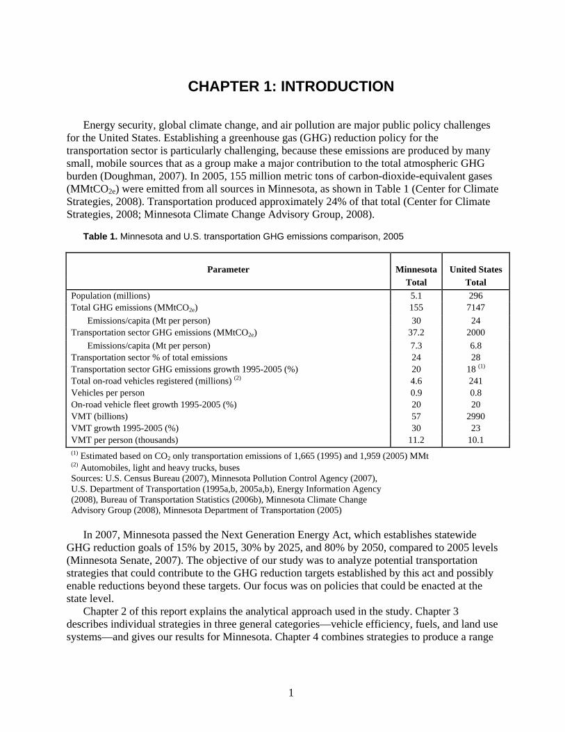
CHAPTER 1: INTRODUCTION Energy security, global climate change, and air pollution are major public policy challenges

for the United States. Establishing a greenhouse gas (GHG) reduction policy for the transportation sector is particularly challenging, because these emissions are produced by many small, mobile sources that as a group make a major contribution to the total atmospheric GHG burden (Doughman, 2007). In 2005, 155 million metric tons of carbon-dioxide-equivalent gases (MMtCO2e) were emitted from all sources in Minnesota, as shown in Table 1 (Center for Climate Strategies, 2008). Transportation produced approximately 24% of that total (Center for Climate Strategies, 2008; Minnesota Climate Change Advisory Group, 2008).

Table 1. Minnesota and U.S. transportation GHG emissions comparison, 2005

Parameter

Minnesota

United States

Total Total Population (millions) 5.1 296 Total GHG emissions (MMtCO2e) 155 7147 Emissions/capita (Mt per person) 30 24 Transportation sector GHG emissions (MMtCO2e) 37.2 2000 Emissions/capita (Mt per person) 7.3 6.8 Transportation sector % of total emissions 24 28 Transportation sector GHG emissions growth 1995-2005 (%) 20 18 (1) Total on-road vehicles registered (millions) (2) 4.6 241 Vehicles per person 0.9 0.8 On-road vehicle fleet growth 1995-2005 (%) 20 20 VMT (billions) 57 2990 VMT growth 1995-2005 (%) 30 23 VMT per person (thousands) 11.2 10.1 (1) Estimated based on CO2 only transportation emissions of 1,665 (1995) and 1,959 (2005) MMt (2) Automobiles, light and heavy trucks, buses Sources: U.S. Census Bureau (2007), Minnesota Pollution Control Agency (2007), U.S. Department of Transportation (1995a,b, 2005a,b), Energy Information Agency (2008), Bureau of Transportation Statistics (2006b), Minnesota Climate Change Advisory Group (2008), Minnesota Department of Transportation (2005)

In 2007, Minnesota passed the Next Generation Energy Act, which establishes statewide

GHG reduction goals of 15% by 2015, 30% by 2025, and 80% by 2050, compared to 2005 levels (Minnesota Senate, 2007). The objective of our study was to analyze potential transportation strategies that could contribute to the GHG reduction targets established by this act and possibly enable reductions beyond these targets. Our focus was on policies that could be enacted at the state level.

Chapter 2 of this report explains the analytical approach used in the study. Chapter 3 describes individual strategies in three general categories—vehicle efficiency, fuels, and land use systems—and gives our results for Minnesota. Chapter 4 combines strategies to produce a range

2

of GHG reductions for 2015 and 2025, while Chapter 5 outlines technologies and strategies that show promise for 2050. Chapter 6 presents our conclusions.

Although the statute did not specify reduction targets for individual sectors, our analysis assumes that reductions for transportation would follow the percent reduction guidelines stated above. A full analysis of all sectors would allow allocation of individual sector goals based on cost-effectiveness; that analysis is outside the scope of our transportation-only study.

Federal Regulations and State Policies At present, conventional pollutants such as particulate matter are regulated via emission and

ambient concentration standards. Most GHGs, however, are not currently regulated. GHG pollutants include carbon dioxide (CO2—the main contributor to anthropogenic climate change), methane, nitrous oxide, sulfur hexafluoride, hydrofluorocarbons, perfluorocarbons, chlorofluorocarbons, ozone, and black carbon.

Previous air pollution regulation in the United States has focused on emission and concentration standards for pollutants with known health effects. Transportation-related pollutants such as carbon monoxide, oxides of nitrogen, hydrocarbons, and particulate matter cause health problems and are regulated by states and by the federal government. In contrast, CO2 does not cause direct health problems at typical outdoor concentrations, and emission controls to directly remove CO2 from vehicle exhaust are not commercially available. The lack of exhaust aftertreatment technology for CO2 reduction means that the CO2 mass emission rate must be lowered by consuming less fuel or by lowering fuel carbon content.

Minnesota has enacted a range of energy policies aimed at reducing GHG emissions and increasing biofuel production. In 1997, the state mandated that gasoline contain 10% ethanol (E10). Recently Minnesota requested an EPA waiver to increase the ethanol percentage to 20% by 2013. The 1997 law also requires that diesel fuel contain 2% biodiesel (B2); recent legislation increases the percentage in gradual increments to 20% by 2015. These actions make Minnesota one of the largest consumers of agricultural fuels (biofuels produced from agricultural products such as corn and soybeans).

Other Minnesota laws enacted in 2007 call for plug-in hybrid technology, multimillion-dollar investment in transportation-related research in biofuels, and funding to double the number of E85 (85% ethanol) fuel stations in the state. Legislation also established the Minnesota Climate Change Advisory Group (MCCAG) to provide broad stakeholder input into recommendations on how the state’s GHG emissions could be reduced in all sectors (Minnesota Climate Change Advisory Group, 2008).

Trends Affecting Minnesota’s Transportation GHG Emissions Minnesota ranks fourth among states in terms of ethanol production—one billion gallons

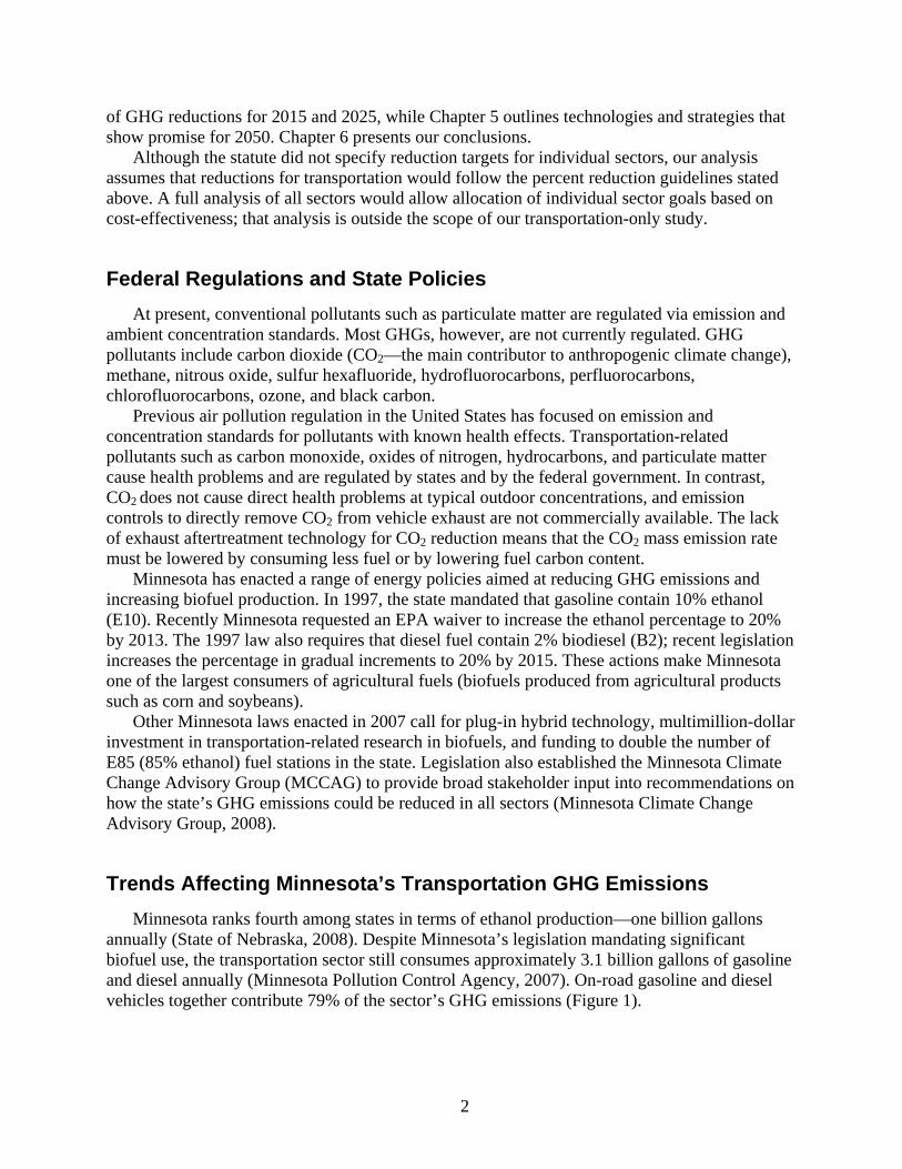
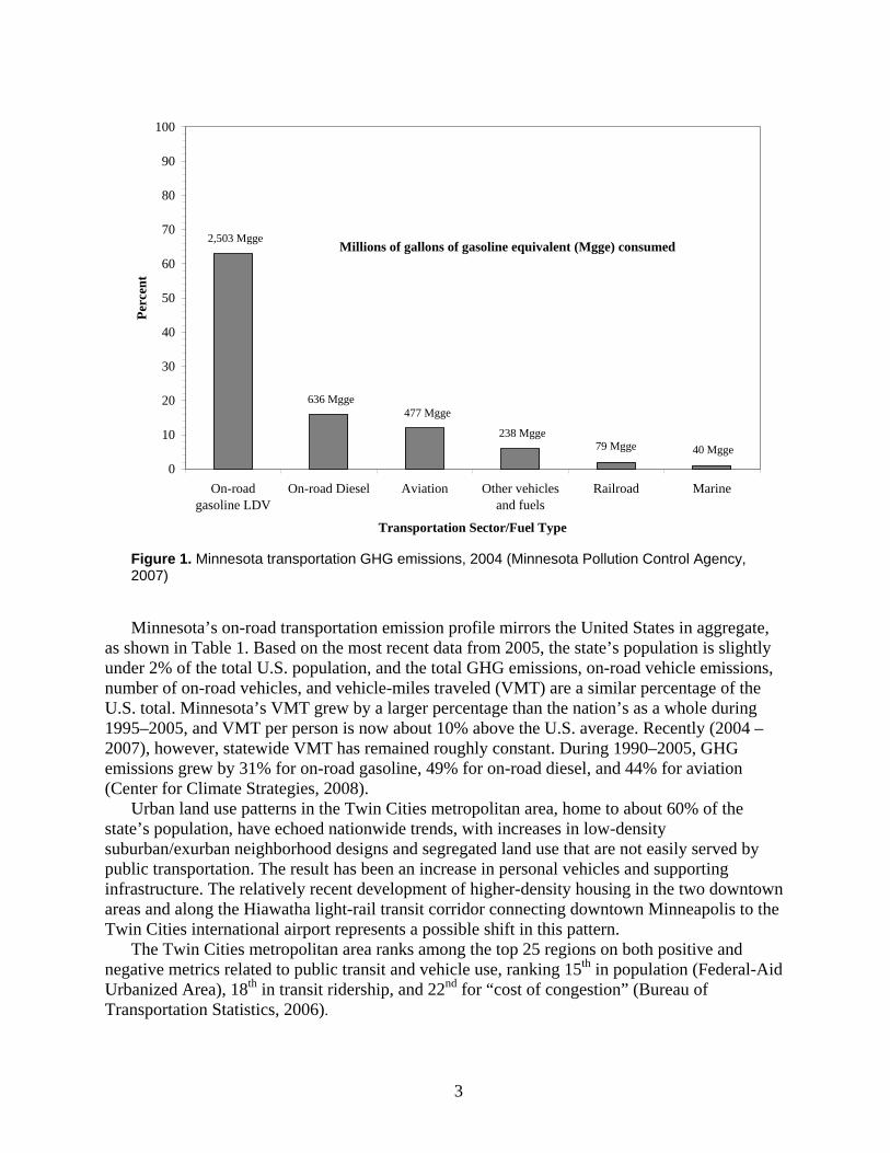
annually (State of Nebraska, 2008). Despite Minnesota’s legislation mandating significant biofuel use, the transportation sector still consumes approximately 3.1 billion gallons of gasoline and diesel annually (Minnesota Pollution Control Agency, 2007). On-road gasoline and diesel vehicles together contribute 79% of the sector’s GHG emissions (Figure 1).

3

0

10

20

30

40

50

60

70

80

90

100

On-roadgasoline LDV

On-road Diesel Aviation Other vehiclesand fuels

Railroad Marine

Transportation Sector/Fuel Type

Perc

ent

2,503 Mgge

636 Mgge 477 Mgge

238 Mgge 79 Mgge 40 Mgge

Millions of gallons of gasoline equivalent (Mgge) consumed

Figure 1. Minnesota transportation GHG emissions, 2004 (Minnesota Pollution Control Agency, 2007) Minnesota’s on-road transportation emission profile mirrors the United States in aggregate,

as shown in Table 1. Based on the most recent data from 2005, the state’s population is slightly under 2% of the total U.S. population, and the total GHG emissions, on-road vehicle emissions, number of on-road vehicles, and vehicle-miles traveled (VMT) are a similar percentage of the U.S. total. Minnesota’s VMT grew by a larger percentage than the nation’s as a whole during 1995–2005, and VMT per person is now about 10% above the U.S. average. Recently (2004 – 2007), however, statewide VMT has remained roughly constant. During 1990–2005, GHG emissions grew by 31% for on-road gasoline, 49% for on-road diesel, and 44% for aviation (Center for Climate Strategies, 2008).

Urban land use patterns in the Twin Cities metropolitan area, home to about 60% of the state’s population, have echoed nationwide trends, with increases in low-density suburban/exurban neighborhood designs and segregated land use that are not easily served by public transportation. The result has been an increase in personal vehicles and supporting infrastructure. The relatively recent development of higher-density housing in the two downtown areas and along the Hiawatha light-rail transit corridor connecting downtown Minneapolis to the Twin Cities international airport represents a possible shift in this pattern.

The Twin Cities metropolitan area ranks among the top 25 regions on both positive and negative metrics related to public transit and vehicle use, ranking 15th in population (Federal-Aid Urbanized Area), 18th in transit ridership, and 22nd for “cost of congestion” (Bureau of Transportation Statistics, 2006).

4

5

CHAPTER 2: ANALYTICAL APPROACH The climate’s response to GHG emissions largely depends on their cumulative concentration

in the atmosphere. While specific-year GHG reduction targets are appropriate for policy implementation, cumulative emissions ultimately determine overall GHG atmospheric concentrations and the resulting impact on climatic conditions.

A common analytic approach is a “wedges” analysis (Socolow and Pacala, 2004), in which two scenarios are generated: the reference case (“business as usual”) and a case that meets a certain objective. The difference between the two scenarios is divided into several “wedges,” each representing a specific mitigation action. The cumulative emission reduction from all “wedges” equals the difference between the desired and the reference scenario.

Our approach is similar to the wedges approach in that we explore sets of solutions that combine to meet a specific objective; an important difference is that we focus on the legislative mandates (reductions of 15% by 2015, 30% by 2025, and 80% by 2050 compared to 2005 levels). Our calculations estimate GHG emissions using the following equation (Mui, et al. 2007):

44 344 214342143421ActivityContentCarbon nConsumptio Fuel

Traveled Miles Vehicle

GallonCarbon

MileGallons=Emissions ⎟⎟

⎠

⎞⎜⎜⎝

⎛×⎟⎠⎞

⎜⎝⎛×⎟

⎠⎞

⎜⎝⎛

A C F =E ××

Each of the three factors in the equation—per-mile fuel consumption (F), fuel carbon content

(C) and VMT (A)—contributes to overall emissions. Thus, reductions in one parameter may be offset by increases in another. Comprehensive GHG policies will consider all three factors.

A further consideration is the time delay between an action and the resulting emissions reduction. Some actions, such as reducing the fuel carbon content, would generate immediate reductions; in contrast, urban densification may take years before measurable GHG reductions are observed. Our analyses quantify reductions that occur in the short term (2015) and medium term (2025); longer-term impacts (past 2030) are addressed qualitatively.

Our vehicle options examine policies that encourage increased fuel efficiencies through a variety of technical and regulatory initiatives. The fuel options focus on lowering the carbon content of fuels through various mandates, technology shifts, and economic incentives. Land use and system shift options focus on reducing VMT via increased use of alternative travel modes and also through mixed-use and high-density urban design.

Impacts of vehicle and fuel strategies on Minnesota’s GHG emissions were modeled using the Long-Range Energy Alternatives Planning (LEAP) system, an integrated energy-environment modeling tool designed by the Stockholm Environment Institute (Heaps, 2008). The land use and system shift analyses employed published data and a spreadsheet developed by the Center for Clean Air Policy (CCAP, 2006). A report from the Urban Land Institute and Smart Growth America (ULI-SGA) (Ewing, et al., 2007) presented a useful synthesis of existing Smart Growth literature. Our calculations, however, do not follow those given in the ULI-SGA because ULI-SGA reported significantly larger emission-reductions than does CCAP. We chose to rely

6

on the more conservative (that is, lower-magnitude) estimates derived from CCAP. Methods employed by the Minnesota Climate Change Advisory Group (MCCAG) were also consulted, but not used explicitly in this report.

7

CHAPTER 3: INDIVIDUAL STRATEGIES

Light-Duty Vehicle Strategies Minnesota’s light-duty vehicle (LDV) fleet produced approximately 63% (26 MMtCO2e) of

the 2004 transportation GHG emissions (Minnesota Pollution Control Agency, 2007). Reducing total LDV fleet emissions is a function of the number of vehicles, miles traveled per vehicle, and the average emissions per vehicle-mile.

The average emissions per mile can be reduced if vehicles are replaced with lower-emitting models. However, reducing only average emissions per mile may not reduce total fleet emissions because an increase in the number of vehicles or in the number of miles traveled per vehicle could offset vehicle efficiency improvements. Policies to reduce GHG emission per vehicle are most effective, therefore, when enacted with those that reduce the other two factors—fuels and VMT—in parallel.

Emissions and Mileage Standards

California Standards and U.S. CAFE Under the federal Clean Air Act, California (with EPA approval) may establish emission

standards, and any state has the option of adopting the EPA-approved California standards (Environmental Protection Agency, 2008). California has proposed standards for the average GHG emissions of manufacturer fleets (also called California Clean Car, “Pavley” Standards, or California Air Resources Board GHG Regulations) for two categories of LDVs as part of its Low Emission Vehicle (LEV) II rules, with a phase-in schedule from 2009 to 2016 and a planned extension from 2017 to 2020 (California Attorney General's Office, 2007).

Recent developments have affected the implementation of the California standards. In late 2007, Congress enacted the Energy Independence and Security Act that requires Corporate Average Fuel Economy standards (CAFE) for each manufacturer’s fleet to reach 35 MPG by 2020. (CAFE standards have not been increased for cars since 1985.) CAFE standards will reduce GHG emissions per mile from the LDV fleet. The standard also includes provisions for flex-fuel credits and credit trading between vehicle categories and between manufacturers. For example, with flex-fuel credits a manufacturer with an average fuel economy below the target for a particular year could still satisfy CAFE standards. Our analyses include the maximum allowable credits for flex-fuel vehicles.

After passage of the act, the EPA declined to grant a waiver for California’s standards. California and 17 states including Minnesota are currently challenging the EPA decision in court (Wald, 2008).

In April 2008, the National Highway Traffic Safety Administration (NHTSA) published a proposed phase-in schedule for the CAFE standards through 2015 (National Highway Traffic Safety Administration, 2008). This new schedule is more aggressive than previously predicted, with significant fuel economy increases required in the early years. The aggressiveness of the NHTSA schedule reduces the difference in projected emissions between the California and the CAFE standards. Figure 2 shows a projection of the impact on Minnesota LDV emissions of the

8

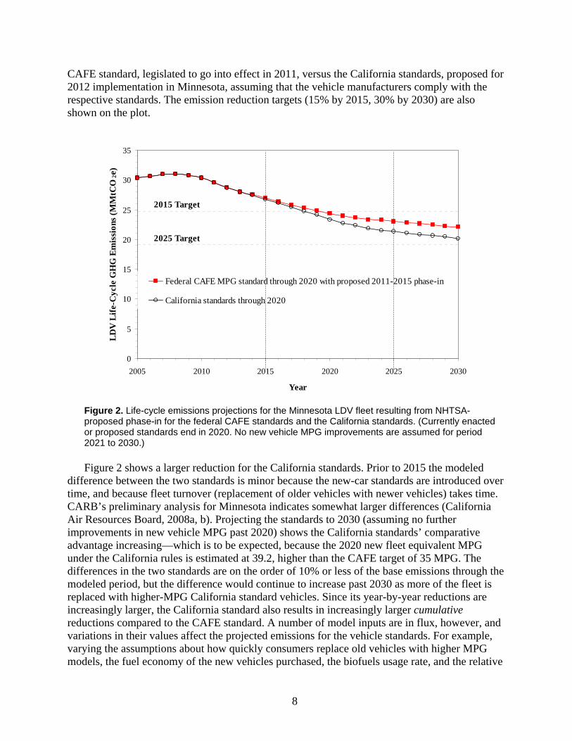
CAFE standard, legislated to go into effect in 2011, versus the California standards, proposed for 2012 implementation in Minnesota, assuming that the vehicle manufacturers comply with the respective standards. The emission reduction targets (15% by 2015, 30% by 2030) are also shown on the plot.

0

5

10

15

20

25

30

35

2005 2010 2015 2020 2025 2030

Year

LDV

Life

-Cyc

le G

HG

Em

issi

ons (

MM

tCO

2e)

Federal CAFE MPG standard through 2020 with proposed 2011-2015 phase-in

California standards through 2020

2015 Target

2025 Target

Figure 2. Life-cycle emissions projections for the Minnesota LDV fleet resulting from NHTSA-proposed phase-in for the federal CAFE standards and the California standards. (Currently enacted or proposed standards end in 2020. No new vehicle MPG improvements are assumed for period 2021 to 2030.) Figure 2 shows a larger reduction for the California standards. Prior to 2015 the modeled

difference between the two standards is minor because the new-car standards are introduced over time, and because fleet turnover (replacement of older vehicles with newer vehicles) takes time. CARB’s preliminary analysis for Minnesota indicates somewhat larger differences (California Air Resources Board, 2008a, b). Projecting the standards to 2030 (assuming no further improvements in new vehicle MPG past 2020) shows the California standards’ comparative advantage increasing—which is to be expected, because the 2020 new fleet equivalent MPG under the California rules is estimated at 39.2, higher than the CAFE target of 35 MPG. The differences in the two standards are on the order of 10% or less of the base emissions through the modeled period, but the difference would continue to increase past 2030 as more of the fleet is replaced with higher-MPG California standard vehicles. Since its year-by-year reductions are increasingly larger, the California standard also results in increasingly larger cumulative reductions compared to the CAFE standard. A number of model inputs are in flux, however, and variations in their values affect the projected emissions for the vehicle standards. For example, varying the assumptions about how quickly consumers replace old vehicles with higher MPG models, the fuel economy of the new vehicles purchased, the biofuels usage rate, and the relative

9

GHG savings of biofuels can increase or decrease the projected emissions under either standard as well as the differences between them (An et al., 2007). Another example is the increased cost of gasoline in the spring of 2008, which has shifted buyers toward more fuel-efficient vehicles (Vasic, 2008); a continuation of that trend would affect how the vehicle fleet is modeled.

U.S. Standards vs. Policies in Other Countries Technologies to achieve the CAFE standard are readily available. Both CAFE and California

standards establish less aggressive mandates than mandates or goals in China, the European Union, and Japan (An, et al., 2004, 2007).

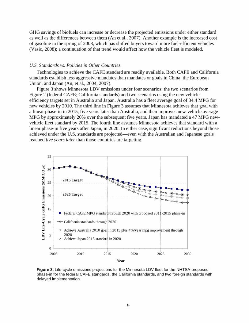
Figure 3 shows Minnesota LDV emissions under four scenarios: the two scenarios from Figure 2 (federal CAFE; California standards) and two scenarios using the new vehicle efficiency targets set in Australia and Japan. Australia has a fleet average goal of 34.4 MPG for new vehicles by 2010. The third line in Figure 3 assumes that Minnesota achieves that goal with a linear phase-in in 2015, five years later than Australia, and then improves new-vehicle average MPG by approximately 20% over the subsequent five years. Japan has mandated a 47 MPG new-vehicle fleet standard by 2015. The fourth line assumes Minnesota achieves that standard with a linear phase-in five years after Japan, in 2020. In either case, significant reductions beyond those achieved under the U.S. standards are projected—even with the Australian and Japanese goals reached five years later than those countries are targeting.

0

5

10

15

20

25

30

35

2005 2010 2015 2020 2025 2030

Year

LDV

Life

-Cyc

le G

HG

Em

issi

ons (

MM

tCO

2e)

Federal CAFE MPG standard through 2020 with proposed 2011-2015 phase-in

California standards through 2020

Achieve Australia 2010 goal in 2015 plus 4%/year mpg improvement through2020Achieve Japan 2015 standard in 2020

2015 Target

2025 Target

Figure 3. Life-cycle emissions projections for the Minnesota LDV fleet for the NHTSA-proposed phase-in for the federal CAFE standards, the California standards, and two foreign standards with delayed implementation

10

Comparisons for China and the EU (not shown) indicate a trend similar to Australia and Japan: Mandated or voluntary standards are more stringent than those proposed for the United States or for the California act. Considered in aggregate, these goals in other major industrialized nations and in China suggest that U.S. standards are weak by international standards. Light-duty vehicle technology development can support larger GHG reductions than are currently being considered in Minnesota and elsewhere in the United States.

Payback Period Estimating the direct cost of implementing standards such as CAFE or California’s requires

assumptions about future fuel costs and the costs of incorporating new technology required to comply with the standards. Forecasting either of those is challenging. Earlier analyses of the impact on California consumers from the adoption of the California standards show a positive benefit, assuming the price of gasoline is $1.74 per gallon (California Air Resources Board, 2005; McManus, 2007). Current gasoline prices would increase the estimated benefit to consumers.

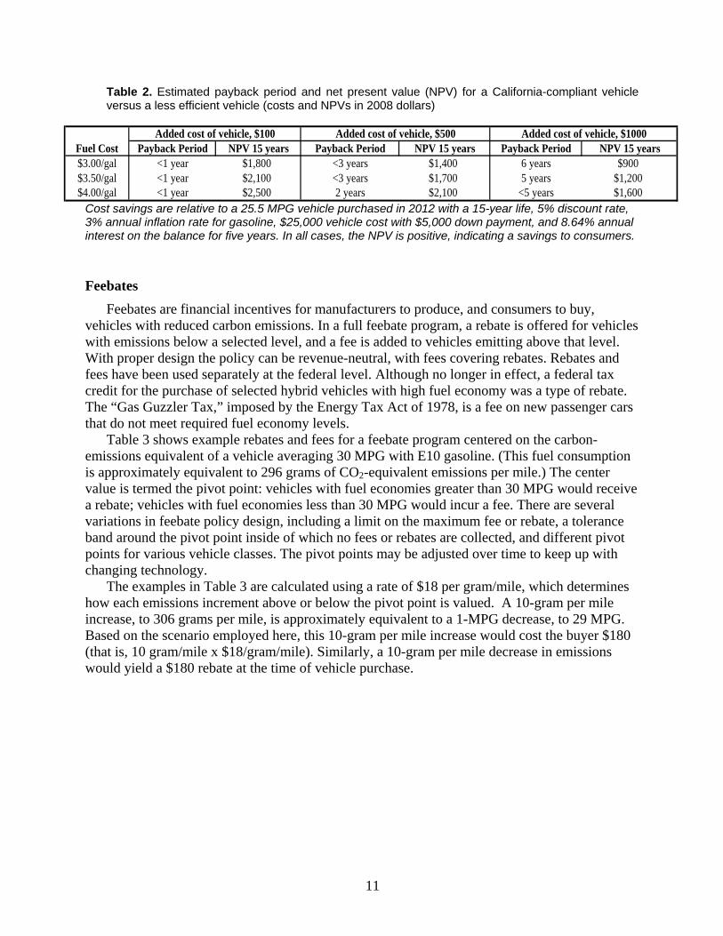
Table 2 shows an estimate of two ways to gauge the financial cost or benefit to a Minnesota consumer in 2012 if a vehicle attaining 29.5 MPG—the equivalent MPG for compliance with the California standards—is purchased instead of a 25.5 MPG vehicle. This analysis used more current gasoline costs of $3.00, $3.50, and $4.00 per gallon (2008 dollars). The additional cost for the higher efficiency vehicle was assumed at $100, $500, and $1,000. This range brackets published estimates for the additional cost of more fuel-efficient new vehicles complying with the California standards in 2012, around which there is uncertainty. CARB and others estimated the costs of meeting the California standard before the enactment of the new CAFE standards. New CAFE will increase the baseline fleet MPG, which should reduce the incremental cost needed to meet the California standards and place those costs toward the lower part of the range. Vehicle manufacturers, however, have argued that the CARB estimates are low, and the upper part of the range reflects that position. Nonetheless, even the upper end of the additional cost range, $1000, results in a net benefit to the consumer (California Air Resources Board, 2005 and Subin, 2007).

Table 2 shows that the payback period for the added cost of the higher efficiency vehicle ranges from less than a year to six years, and the net present values (NPV) of the savings for a 15-year vehicle life range between positive $900 and $2,500. In short, the higher efficiency vehicle not only reduces GHG emissions, it also provides a significant net savings in short to intermediate payback periods. Estimating the impact of purchasing a vehicle later in the phase-in period of the two standards (for example, in 2020) requires better information about the cost differences between vehicles meeting the proposed standards compared to vehicles with lower MPG.

11

Table 2. Estimated payback period and net present value (NPV) for a California-compliant vehicle versus a less efficient vehicle (costs and NPVs in 2008 dollars)

Fuel Cost Payback Period NPV 15 years Payback Period NPV 15 years Payback Period NPV 15 years$3.00/gal <1 year $1,800 <3 years $1,400 6 years $900$3.50/gal <1 year $2,100 <3 years $1,700 5 years $1,200$4.00/gal <1 year $2,500 2 years $2,100 <5 years $1,600

Added cost of vehicle, $500 Added cost of vehicle, $1000Added cost of vehicle, $100

Cost savings are relative to a 25.5 MPG vehicle purchased in 2012 with a 15-year life, 5% discount rate, 3% annual inflation rate for gasoline, $25,000 vehicle cost with $5,000 down payment, and 8.64% annual interest on the balance for five years. In all cases, the NPV is positive, indicating a savings to consumers.

Feebates Feebates are financial incentives for manufacturers to produce, and consumers to buy,

vehicles with reduced carbon emissions. In a full feebate program, a rebate is offered for vehicles with emissions below a selected level, and a fee is added to vehicles emitting above that level. With proper design the policy can be revenue-neutral, with fees covering rebates. Rebates and fees have been used separately at the federal level. Although no longer in effect, a federal tax credit for the purchase of selected hybrid vehicles with high fuel economy was a type of rebate. The “Gas Guzzler Tax,” imposed by the Energy Tax Act of 1978, is a fee on new passenger cars that do not meet required fuel economy levels.

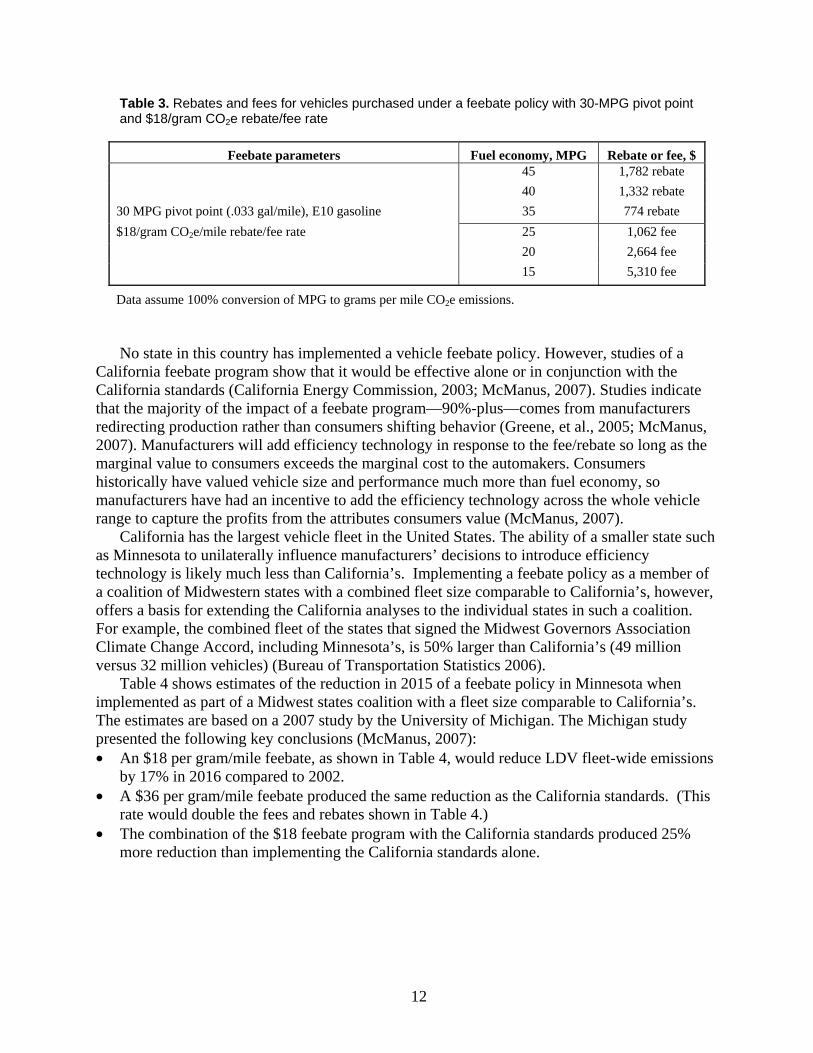
Table 3 shows example rebates and fees for a feebate program centered on the carbon-emissions equivalent of a vehicle averaging 30 MPG with E10 gasoline. (This fuel consumption is approximately equivalent to 296 grams of CO2-equivalent emissions per mile.) The center value is termed the pivot point: vehicles with fuel economies greater than 30 MPG would receive a rebate; vehicles with fuel economies less than 30 MPG would incur a fee. There are several variations in feebate policy design, including a limit on the maximum fee or rebate, a tolerance band around the pivot point inside of which no fees or rebates are collected, and different pivot points for various vehicle classes. The pivot points may be adjusted over time to keep up with changing technology.

The examples in Table 3 are calculated using a rate of $18 per gram/mile, which determines how each emissions increment above or below the pivot point is valued. A 10-gram per mile increase, to 306 grams per mile, is approximately equivalent to a 1-MPG decrease, to 29 MPG. Based on the scenario employed here, this 10-gram per mile increase would cost the buyer $180 (that is, 10 gram/mile x $18/gram/mile). Similarly, a 10-gram per mile decrease in emissions would yield a $180 rebate at the time of vehicle purchase.

12

Table 3. Rebates and fees for vehicles purchased under a feebate policy with 30-MPG pivot point and $18/gram CO2e rebate/fee rate

Feebate parameters Fuel economy, MPG Rebate or fee, $ 45 1,782 rebate 40 1,332 rebate 30 MPG pivot point (.033 gal/mile), E10 gasoline 35 774 rebate $18/gram CO2e/mile rebate/fee rate 25 1,062 fee 20 2,664 fee 15 5,310 fee

Data assume 100% conversion of MPG to grams per mile CO2e emissions. No state in this country has implemented a vehicle feebate policy. However, studies of a

California feebate program show that it would be effective alone or in conjunction with the California standards (California Energy Commission, 2003; McManus, 2007). Studies indicate that the majority of the impact of a feebate program—90%-plus—comes from manufacturers redirecting production rather than consumers shifting behavior (Greene, et al., 2005; McManus, 2007). Manufacturers will add efficiency technology in response to the fee/rebate so long as the marginal value to consumers exceeds the marginal cost to the automakers. Consumers historically have valued vehicle size and performance much more than fuel economy, so manufacturers have had an incentive to add the efficiency technology across the whole vehicle range to capture the profits from the attributes consumers value (McManus, 2007).

California has the largest vehicle fleet in the United States. The ability of a smaller state such as Minnesota to unilaterally influence manufacturers’ decisions to introduce efficiency technology is likely much less than California’s. Implementing a feebate policy as a member of a coalition of Midwestern states with a combined fleet size comparable to California’s, however, offers a basis for extending the California analyses to the individual states in such a coalition. For example, the combined fleet of the states that signed the Midwest Governors Association Climate Change Accord, including Minnesota’s, is 50% larger than California’s (49 million versus 32 million vehicles) (Bureau of Transportation Statistics 2006).

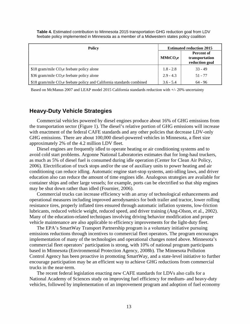
Table 4 shows estimates of the reduction in 2015 of a feebate policy in Minnesota when implemented as part of a Midwest states coalition with a fleet size comparable to California’s. The estimates are based on a 2007 study by the University of Michigan. The Michigan study presented the following key conclusions (McManus, 2007): • An $18 per gram/mile feebate, as shown in Table 4, would reduce LDV fleet-wide emissions

by 17% in 2016 compared to 2002. • A $36 per gram/mile feebate produced the same reduction as the California standards. (This

rate would double the fees and rebates shown in Table 4.) • The combination of the $18 feebate program with the California standards produced 25%

more reduction than implementing the California standards alone.

13

Table 4. Estimated contribution to Minnesota 2015 transportation GHG reduction goal from LDV feebate policy implemented in Minnesota as a member of a Midwestern states policy coalition

Policy Estimated reduction 2015

MMtCO2e

Percent of transportation reduction goal

$18 gram/mile CO2e feebate policy alone 1.8 - 2.8 33 - 49 $36 gram/mile CO2e feebate policy alone 2.9 - 4.3 51 - 77

$18 gram/mile CO2e feebate policy and California standards combined 3.6 - 5.4 64 - 96

Based on McManus 2007 and LEAP model 2015 California standards reduction with +/- 20% uncertainty

Heavy-Duty Vehicle Strategies Commercial vehicles powered by diesel engines produce about 16% of GHG emissions from

the transportation sector (Figure 1). The diesel’s relative portion of GHG emissions will increase with enactment of the federal CAFE standards and any other policies that decrease LDV-only GHG emissions. There are about 100,000 diesel-powered vehicles in Minnesota, a fleet size approximately 2% of the 4.2 million LDV fleet.

Diesel engines are frequently idled to operate heating or air conditioning systems and to avoid cold start problems. Argonne National Laboratories estimates that for long-haul truckers, as much as 5% of diesel fuel is consumed during idle operation (Center for Clean Air Policy, 2006). Electrification of truck stops and/or the use of auxiliary units to power heating and air conditioning can reduce idling. Automatic engine start-stop systems, anti-idling laws, and driver education also can reduce the amount of time engines idle. Analogous strategies are available for container ships and other large vessels; for example, ports can be electrified so that ship engines may be shut down rather than idled (Fournier, 2006).

Commercial trucks can increase efficiency with an array of technological enhancements and operational measures including improved aerodynamics for both trailer and tractor, lower rolling resistance tires, properly inflated tires ensured through automatic inflation systems, low-friction lubricants, reduced vehicle weight, reduced speed, and driver training (Ang-Olson, et al., 2002). Many of the education-related techniques involving driving behavior modification and proper vehicle maintenance are also applicable to efficiency improvements for the light-duty fleet.

The EPA’s SmartWay Transport Partnership program is a voluntary initiative pursuing emissions reductions through incentives to commercial fleet operators. The program encourages implementation of many of the technologies and operational changes noted above. Minnesota’s commercial fleet operators’ participation is strong, with 10% of national program participants based in Minnesota (Environmental Protection Agency, 2008b). The Minnesota Pollution Control Agency has been proactive in promoting SmartWay, and a state-level initiative to further encourage participation may be an efficient way to achieve GHG reductions from commercial trucks in the near-term.

The recent federal legislation enacting new CAFE standards for LDVs also calls for a National Academy of Sciences study on improving fuel efficiency for medium- and heavy-duty vehicles, followed by implementation of an improvement program and adoption of fuel economy

14

standards for these classes. Shifting freight to more efficient modes such as trains is discussed later in this paper.

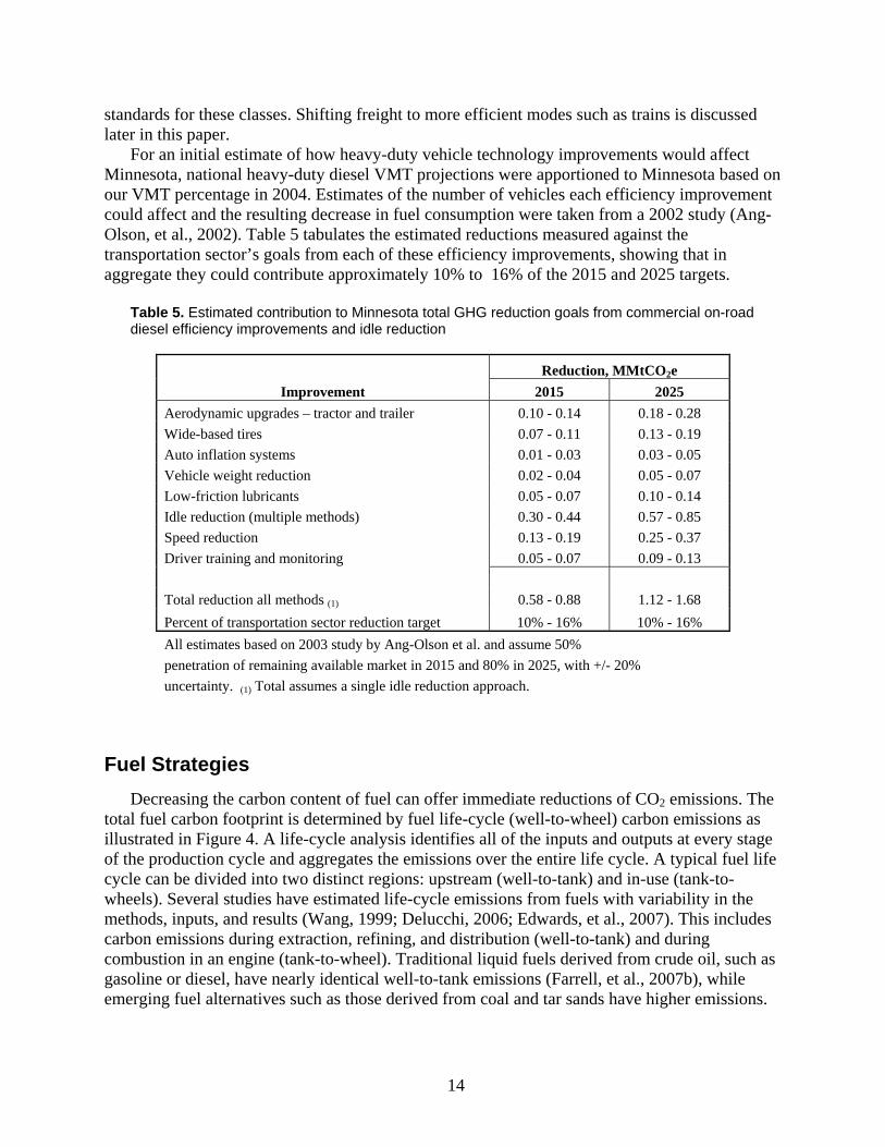
For an initial estimate of how heavy-duty vehicle technology improvements would affect Minnesota, national heavy-duty diesel VMT projections were apportioned to Minnesota based on our VMT percentage in 2004. Estimates of the number of vehicles each efficiency improvement could affect and the resulting decrease in fuel consumption were taken from a 2002 study (Ang-Olson, et al., 2002). Table 5 tabulates the estimated reductions measured against the transportation sector’s goals from each of these efficiency improvements, showing that in aggregate they could contribute approximately 10% to 16% of the 2015 and 2025 targets.

Table 5. Estimated contribution to Minnesota total GHG reduction goals from commercial on-road diesel efficiency improvements and idle reduction

Reduction, MMtCO2e Improvement 2015 2025

Aerodynamic upgrades – tractor and trailer 0.10 - 0.14 0.18 - 0.28 Wide-based tires 0.07 - 0.11 0.13 - 0.19 Auto inflation systems 0.01 - 0.03 0.03 - 0.05 Vehicle weight reduction 0.02 - 0.04 0.05 - 0.07 Low-friction lubricants 0.05 - 0.07 0.10 - 0.14 Idle reduction (multiple methods) 0.30 - 0.44 0.57 - 0.85 Speed reduction 0.13 - 0.19 0.25 - 0.37 Driver training and monitoring 0.05 - 0.07 0.09 - 0.13

Total reduction all methods (1) 0.58 - 0.88 1.12 - 1.68 Percent of transportation sector reduction target 10% - 16% 10% - 16% All estimates based on 2003 study by Ang-Olson et al. and assume 50% penetration of remaining available market in 2015 and 80% in 2025, with +/- 20% uncertainty. (1) Total assumes a single idle reduction approach.

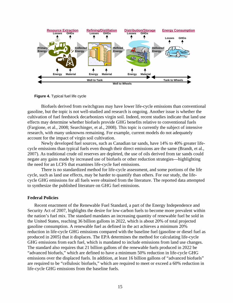
Fuel Strategies Decreasing the carbon content of fuel can offer immediate reductions of CO2 emissions. The

total fuel carbon footprint is determined by fuel life-cycle (well-to-wheel) carbon emissions as illustrated in Figure 4. A life-cycle analysis identifies all of the inputs and outputs at every stage of the production cycle and aggregates the emissions over the entire life cycle. A typical fuel life cycle can be divided into two distinct regions: upstream (well-to-tank) and in-use (tank-to-wheels). Several studies have estimated life-cycle emissions from fuels with variability in the methods, inputs, and results (Wang, 1999; Delucchi, 2006; Edwards, et al., 2007). This includes carbon emissions during extraction, refining, and distribution (well-to-tank) and during combustion in an engine (tank-to-wheel). Traditional liquid fuels derived from crude oil, such as gasoline or diesel, have nearly identical well-to-tank emissions (Farrell, et al., 2007b), while emerging fuel alternatives such as those derived from coal and tar sands have higher emissions.

15

Figure 4. Typical fuel life cycle

Biofuels derived from switchgrass may have lower life-cycle emissions than conventional gasoline, but the topic is not well-studied and research is ongoing. Another issue is whether the cultivation of fuel feedstock decarbonizes virgin soil. Indeed, recent studies indicate that land use effects may determine whether biofuels provide GHG benefits relative to conventional fuels (Fargione, et al., 2008; Searchinger, et al., 2008). This topic is currently the subject of intensive research, with many unknowns remaining. For example, current models do not adequately account for the impact of virgin soil cultivation.

Newly developed fuel sources, such as Canadian tar sands, have 14% to 40% greater life-cycle emissions than typical fuels even though their direct emissions are the same (Brandt, et al., 2007). As traditional crude oil reserves are depleted, the use of oils derived from tar sands could negate any gains made by increased use of biofuels or other reduction strategies—highlighting the need for an LCFS that examines life-cycle fuel emissions.

There is no standardized method for life-cycle assessment, and some portions of the life cycle, such as land use effects, may be harder to quantify than others. For our study, the life-cycle GHG emissions for all fuels were obtained from the literature. The reported data attempted to synthesize the published literature on GHG fuel emissions.

Federal Policies

Recent enactment of the Renewable Fuel Standard, a part of the Energy Independence and Security Act of 2007, highlights the desire for low-carbon fuels to become more prevalent within the nation’s fuel mix. The standard mandates an increasing quantity of renewable fuel be sold in the United States, reaching 36 billion gallons in 2022, which is about 20% of total projected gasoline consumption. A renewable fuel as defined in the act achieves a minimum 20% reduction in life-cycle GHG emissions compared with the baseline fuel (gasoline or diesel fuel as produced in 2005) that it displaces. The EPA determines the method for calculating life-cycle GHG emissions from each fuel, which is mandated to include emissions from land use changes. The standard also requires that 21 billion gallons of the renewable fuels produced in 2022 be “advanced biofuels,” which are defined to have a minimum 50% reduction in life-cycle GHG emissions over the displaced fuels. In addition, at least 16 billion gallons of “advanced biofuels” are required to be “cellulosic biofuels,” which are required to meet or exceed a 60% reduction in life-cycle GHG emissions from the baseline fuels.

Resource Extraction Refining/Distillation Distribution/Storage Energy Consumption

Well to Tank

Tank to Wheels

Well to Wheels

Energy Material Energy Material Energy Material

Losses GHGs Losses GHGs Losses GHGs

Losses GHGs

Primary Energy

Collected Energy

Refined Energy

Delivered Energy

16

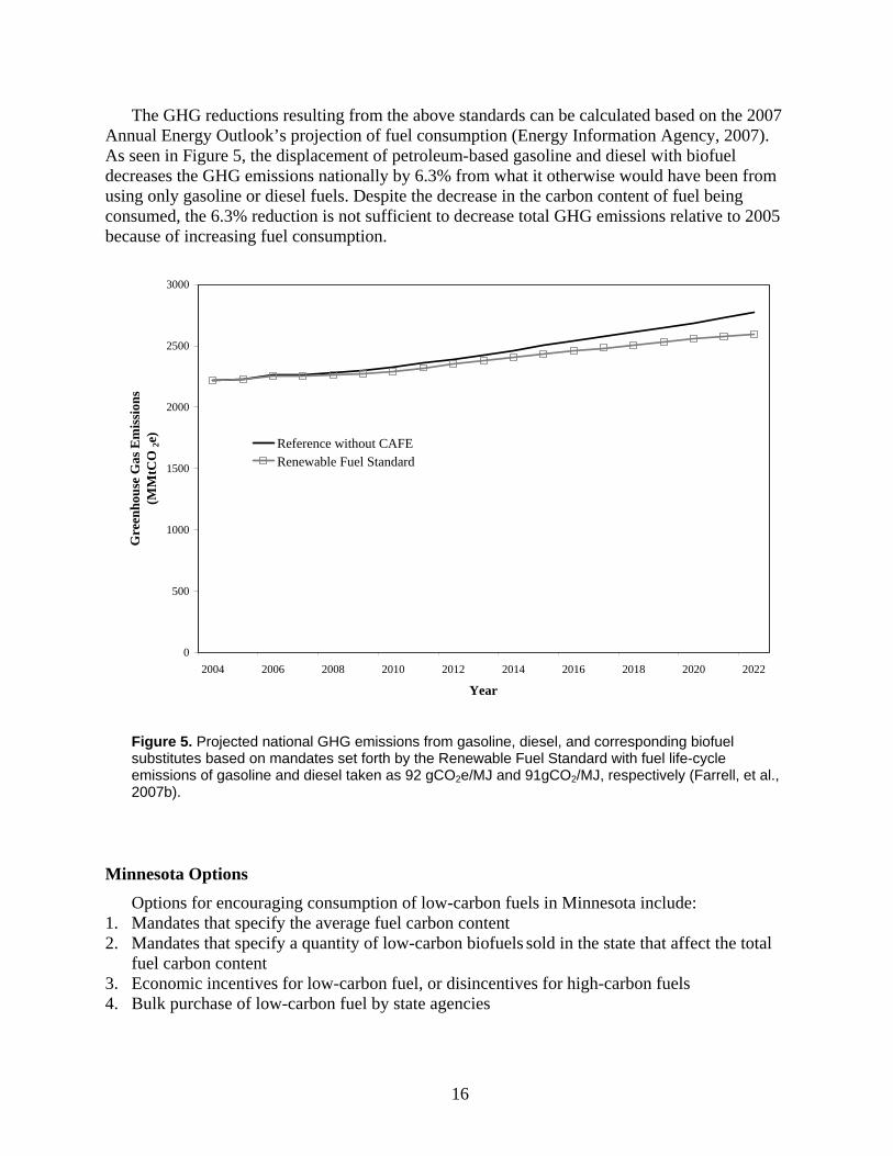
The GHG reductions resulting from the above standards can be calculated based on the 2007 Annual Energy Outlook’s projection of fuel consumption (Energy Information Agency, 2007). As seen in Figure 5, the displacement of petroleum-based gasoline and diesel with biofuel decreases the GHG emissions nationally by 6.3% from what it otherwise would have been from using only gasoline or diesel fuels. Despite the decrease in the carbon content of fuel being consumed, the 6.3% reduction is not sufficient to decrease total GHG emissions relative to 2005 because of increasing fuel consumption.

0

500

1000

1500

2000

2500

3000

2004 2006 2008 2010 2012 2014 2016 2018 2020 2022

Year

Gre

enho

use

Gas

Em

issi

ons

(MM

tCO

2e)

ReferenceRenewable Fuel Standard

without CAFE

Figure 5. Projected national GHG emissions from gasoline, diesel, and corresponding biofuel substitutes based on mandates set forth by the Renewable Fuel Standard with fuel life-cycle emissions of gasoline and diesel taken as 92 gCO2e/MJ and 91gCO2/MJ, respectively (Farrell, et al., 2007b).

Minnesota Options Options for encouraging consumption of low-carbon fuels in Minnesota include:

1. Mandates that specify the average fuel carbon content 2. Mandates that specify a quantity of low-carbon biofuels sold in the state that affect the total

fuel carbon content 3. Economic incentives for low-carbon fuel, or disincentives for high-carbon fuels 4. Bulk purchase of low-carbon fuel by state agencies

17

Options 1 and 2 are discussed next. Options 3 and 4 were not considered owing to time and budget constraints, but they merit further evaluation.

Low-Carbon Fuel Standard A low-carbon fuel standard (LCFS) is a market-based mechanism that requires fuel providers

within the state to reduce fuel carbon content at the pump by a specified percentage over a given period of time. Under an LCFS, fuel providers are required to calculate the carbon intensity of their fuels. Carbon intensity includes total life-cycle emissions, incorporating GHG emissions associated with the production, transportation, and storage of the fuel as well as any land use changes that may have a climate-changing effect. Fuel providers are allowed to reduce the carbon intensity of their fuels by blending them with lower carbon fuels or by purchasing carbon credits from other providers. The result would be a lower statewide average carbon intensity of fuels, which would in turn lower total transportation GHG emissions.

The LCFS approach was endorsed at the Midwestern Governors Association meeting in 2007. California enacted the first LCFS in 2007 (Schwarzenegger, 2007); its mandate requires a 10% reduction in the fuel carbon content by 2020. A detailed analysis of the California LCFS found that a 10% reduction in fuel carbon content was achievable on a state level, and that the LCFS would be best used in conjunction with other policies that seek to increase vehicle efficiency and reduce vehicle-miles traveled (Farrell, et al., 2007a). While our analyses did not seek to repeat the California analysis, we did examine several key issues and determine whether Minnesota could comply with an LCFS, and we give an example of how it could be accomplished.

One of the primary issues in developing an LCFS is defining the average fuel carbon intensity (AFCI) and what the target AFCI should be. Central to the development and implementation of any LCFS is the life-cycle analysis of fuels as discussed above.

A central parameter in our model is GHG emissions per energy content in the fuel, expressed in units of grams of CO2-equivalent per mega joule (g-CO2e/MJ; data for this parameter from Farrell, et al., 2007a). Gasoline, diesel, biofuels, and electricity have emissions greater than zero, indicating net deleterious impact on climate. Some of the biofuels have larger emissions than do gasoline or diesel.

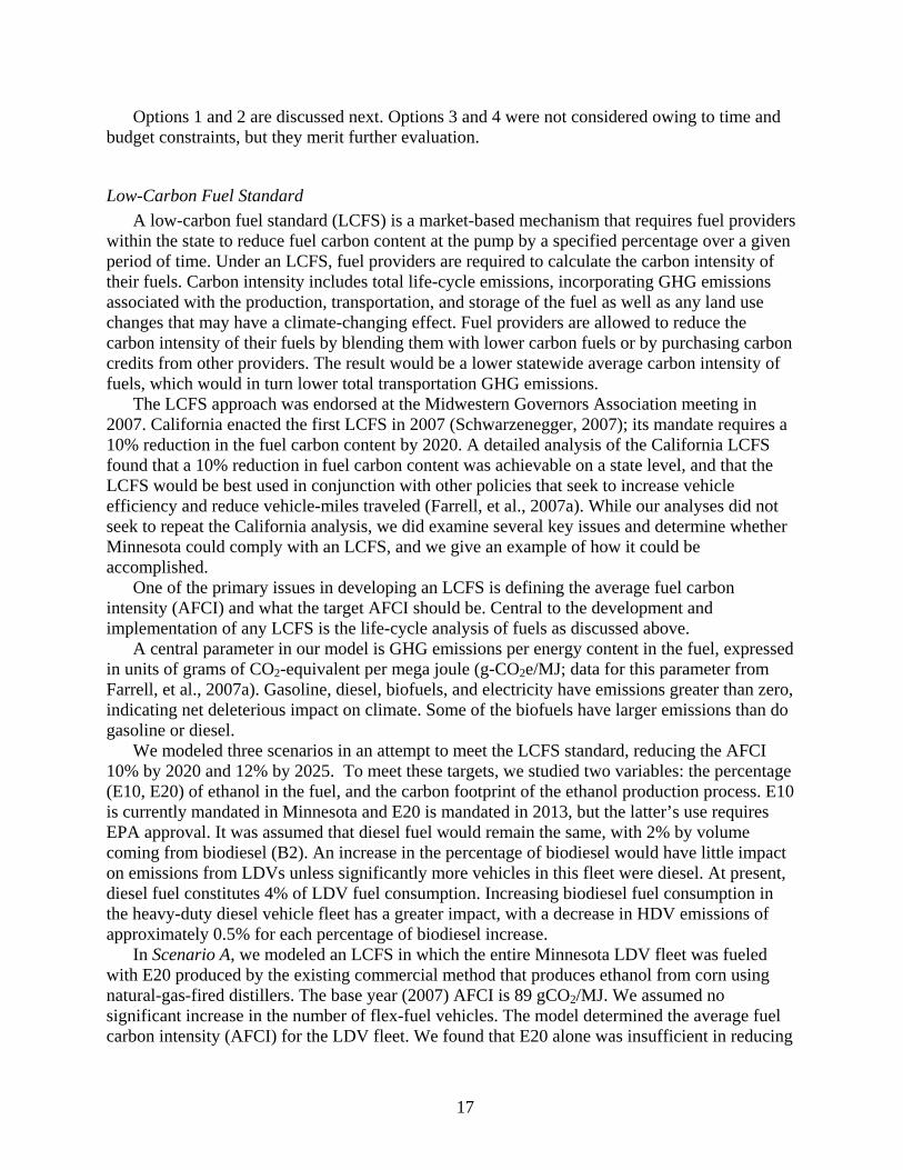
We modeled three scenarios in an attempt to meet the LCFS standard, reducing the AFCI 10% by 2020 and 12% by 2025. To meet these targets, we studied two variables: the percentage (E10, E20) of ethanol in the fuel, and the carbon footprint of the ethanol production process. E10 is currently mandated in Minnesota and E20 is mandated in 2013, but the latter’s use requires EPA approval. It was assumed that diesel fuel would remain the same, with 2% by volume coming from biodiesel (B2). An increase in the percentage of biodiesel would have little impact on emissions from LDVs unless significantly more vehicles in this fleet were diesel. At present, diesel fuel constitutes 4% of LDV fuel consumption. Increasing biodiesel fuel consumption in the heavy-duty diesel vehicle fleet has a greater impact, with a decrease in HDV emissions of approximately 0.5% for each percentage of biodiesel increase.

In Scenario A, we modeled an LCFS in which the entire Minnesota LDV fleet was fueled with E20 produced by the existing commercial method that produces ethanol from corn using natural-gas-fired distillers. The base year (2007) AFCI is 89 gCO2/MJ. We assumed no significant increase in the number of flex-fuel vehicles. The model determined the average fuel carbon intensity (AFCI) for the LDV fleet. We found that E20 alone was insufficient in reducing

18

the carbon content of the fuel because of the lower emissions of average Midwest corn ethanol (76 g CO2e/MJ) with respect to gasoline (92 g CO2e/MJ) (Farrell, et al., 2007a).

Scenario B also assumes E20, but with all ethanol produced from corn using a dry-mill process in a refinery burning stover (leaves and stalks) to make process heat. This process reduces the ethanol portion of carbon emissions from 76 to 47 g CO2e/MJ. Figure 6 shows that a 10% AFCI reduction is achievable by 2020, but the 12% is not because traditional gasoline vehicles will not accept quantities of ethanol in excess of 20%. Minnesota produces enough corn to produce the E20 needed in this scenario (Minnesota Pollution Control Agency, 2008), but using more corn to produce fuel may have adverse consequences, such as conversion of virgin land to cropland both domestically and abroad (Fargione, et al., 2008). In addition, the removal of corn stover from the cropland may contribute to soil degradation (Lal, 2005).

In Scenario C, the ethanol feedstock is switched from corn to cellulosic material, and an E10 blend is assumed. Ethanol produced from cellulosic feedstock was phased in at an assumed rate. By 2020 ethanol produced from cellulosic materials made up over 75% of state ethanol consumption, and 90% by 2025. The benefits from this conversion to cellulosic material from prairie grass, for instance, are derived because there is a greater than 90% reduction in the AFCI from Midwest average corn ethanol (76 gCO2-e/MJ) to cellulosic ethanol derived from Midwest prairie grass (7 gCO2-e/MJ). In this scenario, the 2020 and 2025 targets are met even without changing from E10 to E20, demonstrating the importance of the fuel processing methods and source of biomass. Scenario C shows that the LCFS can be met in Minnesota.

While Scenario C demonstrates that an LCFS can be achieved by increasing the consumption of cellulosic biofuels, many other methods of compliance are possible, including increased dieselization of the LDV fleet, electrification of the fleet with low-carbon electricity, and combinations thereof. Regardless of how the LCFS is met, the net effect on GHG emissions is the same—a 10% reduction in 2020 and 12% reduction in 2025.

19

70

75

80

85

90

2000 2005 2010 2015 2020 2025 2030

Year

AFC

I (gC

O2e

/MJ)

Reference AFCIScenario AScenario BScenario C

10% Reduction - 2020 Target

12% Reduction - 2025 Target

Average fuel carbon intensity (AFCI)

Figure 6. Average fuel carbon intensity (AFCI) for the light-duty vehicle fleet (LDV)

Fuel Mandates Fuel mandates require a specific quantity of fuel or proportion of fuels. Mandates can

increase investment in biofuels and may curb GHG emissions from the transportation sector. However, without any attempt to reduce the carbon footprint of fuels by improving production technology, there is little reduction in GHG emissions. A fuel mandate requiring a switch to E20 and B5 without any carbon reduction standards is equivalent to Scenario A (Figure 6). Results show there is less than a 2% reduction in GHG emissions from corn-based E20 compared to the current E10 despite the fact that twice as much ethanol is consumed. Because the Midwest average corn ethanol has only 17% lower GHG emissions (not accounting for land use changes which could be significant), there is little gained from increasing corn ethanol consumption without a technology mandate to improve the GHG efficiency of ethanol production. Increasing the amount of biodiesel from 2% to 5% has little impact on light-duty fleet CO2 emissions, because few light-duty vehicles use diesel engines.

Land Use and System Shift Strategies Reducing the VMT portion of the E=F×C×A equation is the third broad strategy to reduce

GHG emissions. A well-designed transportation system can reduce vehicle-miles traveled per person (VMTpp) by cutting the distance between travel origins and destinations or by shifting toward more fuel-efficient modes, thus moving people and goods more efficiently.

20

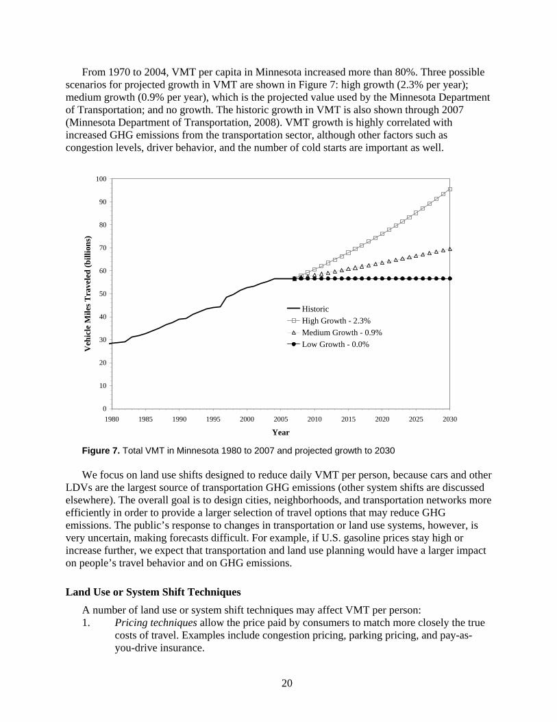
From 1970 to 2004, VMT per capita in Minnesota increased more than 80%. Three possible scenarios for projected growth in VMT are shown in Figure 7: high growth (2.3% per year); medium growth (0.9% per year), which is the projected value used by the Minnesota Department of Transportation; and no growth. The historic growth in VMT is also shown through 2007 (Minnesota Department of Transportation, 2008). VMT growth is highly correlated with increased GHG emissions from the transportation sector, although other factors such as congestion levels, driver behavior, and the number of cold starts are important as well.

0

10

20

30

40

50

60

70

80

90

100

1980 1985 1990 1995 2000 2005 2010 2015 2020 2025 2030

Year

Veh

icle

Mile

s Tra

vele

d (b

illio

ns)

HistoricHigh Growth - 2.3%Medium Growth - 0.9%Low Growth - 0.0%

Figure 7. Total VMT in Minnesota 1980 to 2007 and projected growth to 2030 We focus on land use shifts designed to reduce daily VMT per person, because cars and other

LDVs are the largest source of transportation GHG emissions (other system shifts are discussed elsewhere). The overall goal is to design cities, neighborhoods, and transportation networks more efficiently in order to provide a larger selection of travel options that may reduce GHG emissions. The public’s response to changes in transportation or land use systems, however, is very uncertain, making forecasts difficult. For example, if U.S. gasoline prices stay high or increase further, we expect that transportation and land use planning would have a larger impact on people’s travel behavior and on GHG emissions.

Land Use or System Shift Techniques A number of land use or system shift techniques may affect VMT per person: 1. Pricing techniques allow the price paid by consumers to match more closely the true

costs of travel. Examples include congestion pricing, parking pricing, and pay-as-you-drive insurance.

21

2. Alternative travel modes aim to allow greater choice to consumers to shift to more efficient modes. Examples include carpooling, non-motorized travel (walking/biking), and transit (light-rail transit and bus rapid transit). For shipping freight, GHG emissions per ton-mile are generally lower via boat and rail than via truck and airplane.

3. Supportive land use strategies, network design, and urban form strive to capture benefits associated with linking transportation and land use planning. Strategies include densification, jobs-housing balance, transit-oriented housing, and Smart Growth.

4. Flexible commutes can reduce GHG emissions from commuter-related trips. Examples include telecommuting, flexible or compressed schedules, vanpools and carpools, and guaranteed ride home programs for people who use alternative transportation modes.

5. Process alteration and capacity building aim to increase knowledge about GHG mitigation strategies. Examples include requiring GHG emission estimates in conventional Environmental Impact Statements; creating an Office of Sustainability within the Minnesota Department of Transportation; adjusting funding allocations to account for GHG reduction goals; requiring a “shadow price” for carbon emissions in budgeting for public works projects, thereby allowing decision makers to know whether a hypothetical carbon tax would influence a specific spending decision; and educating the public and private sectors on activities to reduce transportation GHG emissions. A direct carbon tax is discussed below; however, as a process alteration, Minnesota could adopt a trivially small carbon tax (for example, $0.10 per ton), which would be too small to raise significant funds or generate strong direct economic impact, yet would generate new processes and information by requiring emitters to estimate their emissions.

Implementation Challenges Effective implementation of land use and system shift strategies has a number of important challenges: 1. Decentralized decision making. Land use decision making is decentralized, typically

requiring coordination at several levels of government. This can make effective implementation challenging, as competing interests within multiple layers of government strive for different goals. At the same time, decentralized decision making can also present opportunities. For example, well-planned incentives can provide clear market signals for local governments, companies, and individuals.

2. Insufficient funding. Infrastructure development is capital intensive and often requires obtaining federal or state funds through competitive, lengthy, and expensive processes. The uncertainty surrounding future funding at any governmental level creates challenges in project planning and prioritization.

3. Induced demand. Efficiency improvements generally reduce travel times and costs. These improvements often stimulate induced demand: travel increases, thereby reducing the improvement’s effectiveness.

4. Consumer preferences. Minnesotans consider more than just transportation costs when choosing where to live and work and how to travel. Crafting policies that address and recognize these realities is complex. Given the complexity of

22

transportation and land use systems, it is often difficult to measure, estimate, or predict the impact of specific strategies, thereby making choices more difficult.

Transit and Smart Growth Transit is a commonly discussed approach for reducing VMT that illustrates the challenges

that must be overcome for successful implementation. One challenge is development itself: A transit system requires the adoption of a long-term strategy, significant capital, right-of-way procurement, and a commitment by government at all levels.

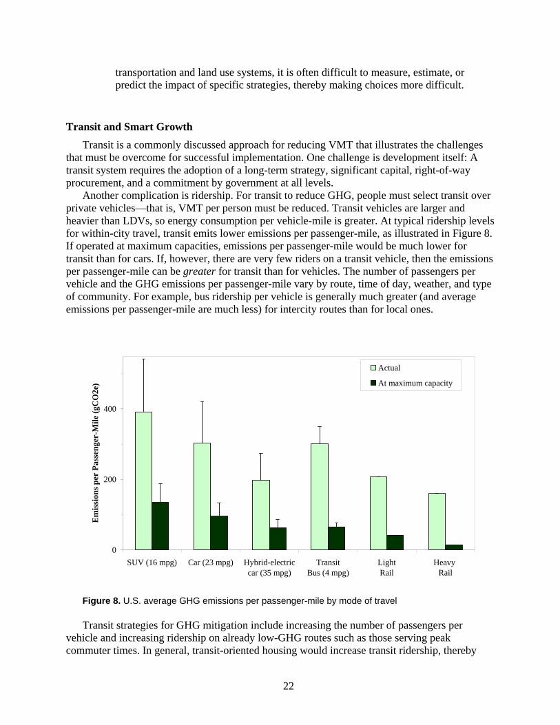
Another complication is ridership. For transit to reduce GHG, people must select transit over private vehicles—that is, VMT per person must be reduced. Transit vehicles are larger and heavier than LDVs, so energy consumption per vehicle-mile is greater. At typical ridership levels for within-city travel, transit emits lower emissions per passenger-mile, as illustrated in Figure 8. If operated at maximum capacities, emissions per passenger-mile would be much lower for transit than for cars. If, however, there are very few riders on a transit vehicle, then the emissions per passenger-mile can be greater for transit than for vehicles. The number of passengers per vehicle and the GHG emissions per passenger-mile vary by route, time of day, weather, and type of community. For example, bus ridership per vehicle is generally much greater (and average emissions per passenger-mile are much less) for intercity routes than for local ones.

0

200

400

SUV (16 mpg) Car (23 mpg) Hybrid-electriccar (35 mpg)

TransitBus (4 mpg)

LightRail

Heavy Rail

Em

issi

ons p

er P

asse

nger

-Mile

(gC

O2e

)

Actual

At maximum capacity

Figure 8. U.S. average GHG emissions per passenger-mile by mode of travel Transit strategies for GHG mitigation include increasing the number of passengers per

vehicle and increasing ridership on already low-GHG routes such as those serving peak commuter times. In general, transit-oriented housing would increase transit ridership, thereby

23

lowering total emissions. In some cases, GHG-mitigation goals will coincide with other transit goals such as increasing ridership. In other cases, the goals may conflict—in which case, transit authorities may need to make trade-offs among competing priorities.

Another strategy for reducing VMT per person is to adopt Smart Growth planning goals. Smart Growth America associates the following goals with the concept “Smart Growth” (Smart Growth America, 2002):

1. Increase the quality, safety, affordability, convenience, and attractiveness of neighborhoods.

2. Improve community access and reduce traffic by mixing land uses that encourage walking, biking and the use of transit.

3. Encourage new development in cities, suburbs, and towns in areas that are already built. 4. Enable equal opportunity and access to benefits that enable residents of all racial and

economic backgrounds to take advantage of the community offerings equally. 5. Promote cost savings through reduced infrastructure requirements and the transportation

choices. 6. Provides public amenities, such as by keeping open space open. Transit-oriented development (TOD) can be an element of Smart Growth. TOD focuses

urban development near light- and heavy-rail stations, with higher population density areas near the station and lower density areas further from the station. Transit stations radiate from downtowns and large employment centers, providing a primary mode of travel in and out of the dense areas. Neighborhoods are built for easy access to stations. Residents in more dense neighborhoods typically drive less each day to reach common destinations (see Figure 9; Marshal et al., 2005; Marshall 2008).

As mentioned elsewhere, densification of urban areas might require less government intervention, not more (Levine, 2006). A commonly held myth in the United States is that neighborhood design and urban development patterns reflect “natural” free markets. In fact, land and transportation markets are highly regulated and experience significant subsidies, fees, and externalities. U.S. developers cite regulation (78%), not insufficient market interest, as the largest barrier to infill development (Levine, 2006).

24

0

10

20

30

40

0 5000 10000 15000 20000

Population Density (people per square mile)

Tra

vel D

ista

nce

(mile

s per

per

son

per

day)

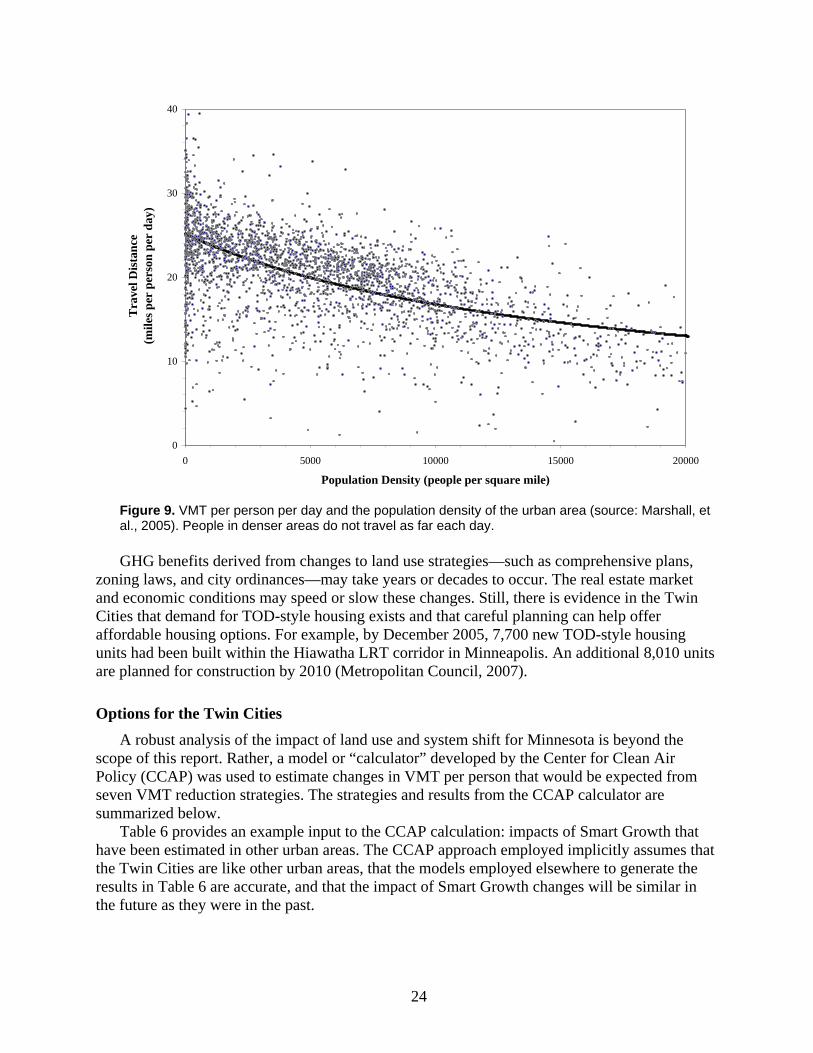
Figure 9. VMT per person per day and the population density of the urban area (source: Marshall, et al., 2005). People in denser areas do not travel as far each day. GHG benefits derived from changes to land use strategies—such as comprehensive plans,

zoning laws, and city ordinances—may take years or decades to occur. The real estate market and economic conditions may speed or slow these changes. Still, there is evidence in the Twin Cities that demand for TOD-style housing exists and that careful planning can help offer affordable housing options. For example, by December 2005, 7,700 new TOD-style housing units had been built within the Hiawatha LRT corridor in Minneapolis. An additional 8,010 units are planned for construction by 2010 (Metropolitan Council, 2007).

Options for the Twin Cities A robust analysis of the impact of land use and system shift for Minnesota is beyond the

scope of this report. Rather, a model or “calculator” developed by the Center for Clean Air Policy (CCAP) was used to estimate changes in VMT per person that would be expected from seven VMT reduction strategies. The strategies and results from the CCAP calculator are summarized below.

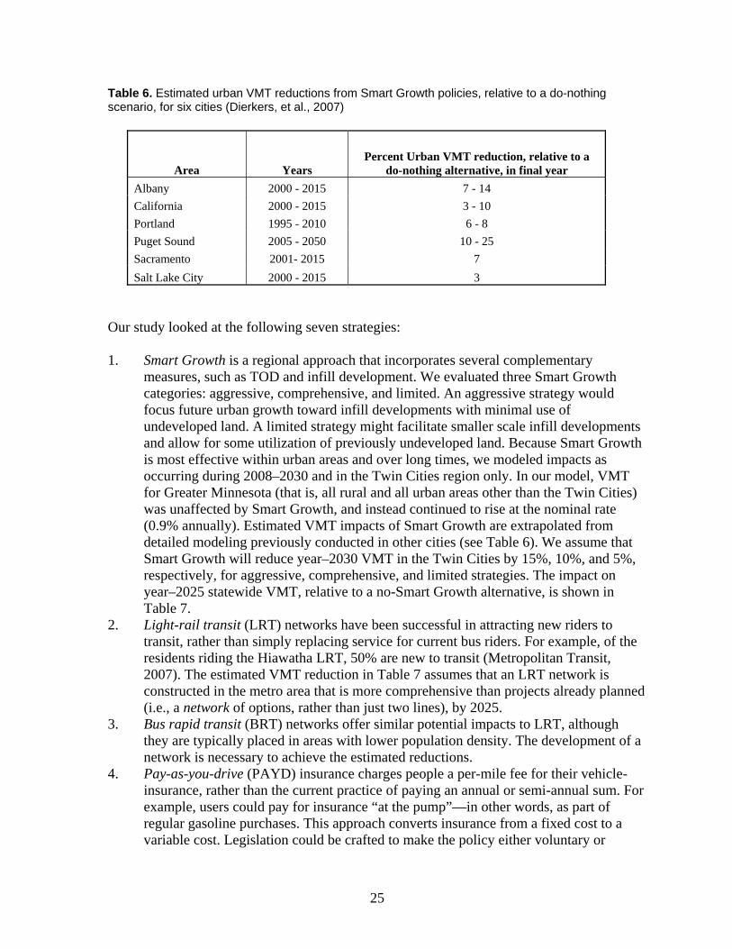
Table 6 provides an example input to the CCAP calculation: impacts of Smart Growth that have been estimated in other urban areas. The CCAP approach employed implicitly assumes that the Twin Cities are like other urban areas, that the models employed elsewhere to generate the results in Table 6 are accurate, and that the impact of Smart Growth changes will be similar in the future as they were in the past.

25

Table 6. Estimated urban VMT reductions from Smart Growth policies, relative to a do-nothing scenario, for six cities (Dierkers, et al., 2007)

Area Years Percent Urban VMT reduction, relative to a

do-nothing alternative, in final year Albany 2000 - 2015 7 - 14 California 2000 - 2015 3 - 10 Portland 1995 - 2010 6 - 8 Puget Sound 2005 - 2050 10 - 25 Sacramento 2001- 2015 7 Salt Lake City 2000 - 2015 3

Our study looked at the following seven strategies: 1. Smart Growth is a regional approach that incorporates several complementary

measures, such as TOD and infill development. We evaluated three Smart Growth categories: aggressive, comprehensive, and limited. An aggressive strategy would focus future urban growth toward infill developments with minimal use of undeveloped land. A limited strategy might facilitate smaller scale infill developments and allow for some utilization of previously undeveloped land. Because Smart Growth is most effective within urban areas and over long times, we modeled impacts as occurring during 2008–2030 and in the Twin Cities region only. In our model, VMT for Greater Minnesota (that is, all rural and all urban areas other than the Twin Cities) was unaffected by Smart Growth, and instead continued to rise at the nominal rate (0.9% annually). Estimated VMT impacts of Smart Growth are extrapolated from detailed modeling previously conducted in other cities (see Table 6). We assume that Smart Growth will reduce year–2030 VMT in the Twin Cities by 15%, 10%, and 5%, respectively, for aggressive, comprehensive, and limited strategies. The impact on year–2025 statewide VMT, relative to a no-Smart Growth alternative, is shown in Table 7.

2. Light-rail transit (LRT) networks have been successful in attracting new riders to transit, rather than simply replacing service for current bus riders. For example, of the residents riding the Hiawatha LRT, 50% are new to transit (Metropolitan Transit, 2007). The estimated VMT reduction in Table 7 assumes that an LRT network is constructed in the metro area that is more comprehensive than projects already planned (i.e., a network of options, rather than just two lines), by 2025.

3. Bus rapid transit (BRT) networks offer similar potential impacts to LRT, although they are typically placed in areas with lower population density. The development of a network is necessary to achieve the estimated reductions.

4. Pay-as-you-drive (PAYD) insurance charges people a per-mile fee for their vehicle-insurance, rather than the current practice of paying an annual or semi-annual sum. For example, users could pay for insurance “at the pump”—in other words, as part of regular gasoline purchases. This approach converts insurance from a fixed cost to a variable cost. Legislation could be crafted to make the policy either voluntary or

26

mandatory. A 10% penetration rate was used to demonstrate potential. Minnesota law does not require PAYD insurance to be offered.

5. Commuter rail lines are constructed on exclusive right-of-ways that have signal priority. They have higher capacity than LRT and BRT but with greater distances between stations, and serve commuters from greater distances. Only the construction of the North Star Commuter Rail from Minneapolis to Big Lake is included in our calculation; additional commuter rail lines would have a larger impact.

6. General transit improvements focus on many small changes to the existing transit system, including construction of additional park-and-ride facilities, provision of transit signal priority, expansion of the guaranteed ride home program, consolidation of transit providers, and a “fix-it first” policy that prioritizes upkeep and maintenance costs relative to costs for new infrastructure.

7. Employer and municipal parking plans pass on to consumers the full cost of parking. There is no such thing as free parking; parking costs are often hidden from consumers, embedded in the cost of other goods and services. Parking plans increase the cost of vehicle commuting by forcing the commuter to pay the full cost of parking. By divorcing the cost of parking from other costs, government officials and private companies are able to charge a market rate for pricing, thereby giving employees more choice in how their transportation funds are used and encouraging other modes of travel. An affected population of 5 percent was used in calculations below.

The estimated VMT reductions from each strategy are not additive reductions, but synergies

and co-benefits may exist. The base case is the medium VMT growth rate (0.9% annually) projected by Minnesota Department of Transportation (see Figure 7). Table 7 summarizes the results in terms of statewide VMT. We assumed that each strategy in Table 7 would be applied to the Twin Cities metropolitan region only, and that there would be no Smart Growth modification in rural areas or in other urban regions of Minnesota. Thus, Table 7 may underestimate the possible statewide impact of each strategy (Dierkers, et al., 2007).

Results in Table 7 are likely to be underestimates. As mentioned above, we assumed Smart Growth changes for the Twin Cities only. Economic factors such as the price of gasoline were not accounted for in our calculations; we expect that Smart Growth strategies will have a larger impact when gasoline prices rise, because consumers have a greater financial incentive to seek alternative modes of travel and to reduce VMT. We also investigated calculations from a report by the Urban Land Institute and Smart Growth America (Ewing, et al., 2007), but chose to employ the more conservative calculations from CCAP rather than those from the ULI-SGA report. The ULI-SGA report suggests a larger impact from Smart Growth than does the CCAP study. This point underscores the challenges and uncertainty behind the quantification of these strategies.

27

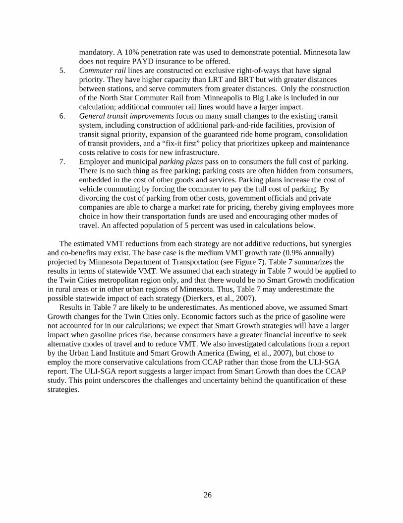
Table 7. Estimated statewide VMT impacts of selected strategies

Strategy Percent Increase in

statewide VMT Percent Statewide year-2025

VMT reduction, 2005 - 2025 relative to a do-nothing scenario

Do-nothing (0.9% annual VMT increase)(1) 19.6 0.0

Smart Growth Aggressive 13.3 5.3 Comprehensive 15.5 3.4 Limited 17.8 1.5 Construction of light-rail transit network 17.0 2.2 Construction of bus rapid transit network 17.0 2.2 Pay-as-you-drive insurance (2) 18.4 1.0 General transit improvements 19.3 0.3 Employer / municipal parking-pricing plans 19.3 0.3

Construction of commuter rail 19.5 0.1 (1) Statewide VMT in 2005 was 57.0 billion. For a do-nothing scenario (0.9% annual VMT increase),

statewide VMT in 2025 is 68.3 billion, a 19.6% increase relative to 2005. For a scenario with aggressive Smart Growth in the Twin Cities, statewide VMT in 2025 is 64.7 billion, a 13.3% increase relative to 2005. Aggressive Smart Growth in the Twin Cities lowers statewide VMT by 5.3% (64.7 billion vs. 68.3 billion).

The aggressive Smart Growth scenario assumed the following. For locations outside the Twin Cites, VMT increased according to a do-nothing scenario (0.9% per year). For the Twin Cities, year-2030 VMT is 15% less than it would be for a do-nothing scenario (based on a linear phase-in from 2007-2030, year-2025 VMT is 11.5% less than with do-nothing). The net effect is that outside the Twin Cities, VMT increases from 30.6 billion in 2005 to 36.6 billion in 2025; in the Twin Cities, VMT increases from 26.5 billion in 2005 to 28.0 billion in 2025 with Smart Growth instead of 31.7 billion in 2025 without Smart Growth.

(2) All options in Table 7 except PAYD were assumed to be implemented in the Twin Cities only. PAYD was assumed to have 10% statewide penetration.

Other Strategies Several strategies for reducing GHG emissions were not analyzed. For example, two that

could apply to transportation and other emission sources are cap-and-trade and a carbon tax. Cap-and-trade policies establish the total allowable quantity of carbon emissions. Companies

may trade carbon credits, and the market—rather than the government—determines prices. A carbon tax policy allows the government to establish the price for carbon emissions while the market determines the quantity of carbon emissions. Cap-and-trade policies have the advantage of greater certainty regarding the quantity of carbon emissions, but emissions from specific sources must be tracked, so implementation is more suited to markets with a small number of large emitters like power plants rather than a large number of small emitters like vehicles.

A carbon tax is conceptually easier to implement because most states already have a sales tax, but it suffers the disadvantage that the emissions and environmental impact are unknown. In general, taxes work well when alternatives are available, as is the case with electricity generation (because many fuel options are readily available). A carbon tax, however, has a more limited

28

application in transportation, because of the limited choice in the selection of fuels and modes of transportation.

Both the cap-and-trade scheme and the carbon tax have appealing qualities but present implementation challenges at a state level. These strategies also entail a number of fundamental policy design considerations with important implications. In the case of a cap-and-trade policy, for example, a basic consideration is where emissions accounting takes place and where the obligation is imposed to supply allowances equal to these emissions. Given the millions of individual emitters in the transportation sector, placing a cap upstream (at the refinery) as opposed to downstream (with the vehicle and fuel consumer) has significant impacts for transaction costs and policy management. Within an upstream system, consumers see the effects of the policy much as they would a tax on fuel. Integration into a transportation cap-and-trade scheme with existing vehicle emissions/MPG standards such as CAFE is another aspect that must be carefully designed to avoid inefficiencies and inequities (Ellerman, et al., 2006).

National and even international leadership for these types of arrangements may yield the largest reductions. These strategies may affect Minnesota in the future and therefore merit mention for that reason.

29

CHAPTER 4: COMBINED STRATEGIES TO MEET THE 2015 AND 2025 GOALS

Combining individual strategies increases the overall reduction in GHG emissions. The

scenarios below evaluate both individual and combined strategies for Minnesota.

Parameters Federal and state agency data for VMT, new vehicle sales, and other factors were used to

project the analysis to 2030. Baseline life-cycle GHG emissions for light-duty vehicles are estimated at 30.4 MMtCO2e for 2005, and transportation’s share of the Minnesota reduction goals is estimated at 5.6 and 11.2 MMtCO2e in 2015 and 2025, respectively. Our reference scenario uses the Minnesota Department of Transportation’s 0.9% per year projected VMT growth for Minnesota.

Figure 10 and Table 8 compare the following individual and combined strategies: 1. New federal CAFE standards with the recently announced phase-in schedule for 2011 to

2015, and assuming continuing increases in new vehicle MPG (2% annual) after the final CAFE year of 2020

2. California standards, also assuming continuing new vehicle MPG improvements (2% annual) after the final year of 2020

3. Low-carbon fuel standard (LCFS) combined with the new federal CAFE standard 4. Comprehensive transportation and land use planning (TLUP) combined with the new

federal CAFE standard 5. California standards, LCFS, and comprehensive transportation and land use planning GHG estimates employ fuel life-cycle GHG emission data. The land use planning estimate is

for the “comprehensive” scenario discussed above. Table 8 provides estimated emission reductions relative to 2005 resulting from each policy or combination and the percentage of the targeted reductions from transportation for 2015 and 2025.

Projections for Minnesota The mandated 2015 and 2025 GHG reduction goals are nearly met in 2015 and are exceeded

in 2025 with the strategy combination of the California standards, the LCFS, and comprehensive transportation and land use planning, assuming the 0.9% VMT growth rate projected by the Minnesota Department of Transportation. However, the scenarios shown in Figure 10 can be significantly altered by the VMT growth assumption, as discussed in the next section. The scenarios are examples of what can be achieved with individual strategies or combinations, focusing primarily on LDV emissions. Further reductions are possible from transportation areas not modeled in the example scenarios, such as from heavy-duty on-road vehicles and aircraft efficiency improvements.

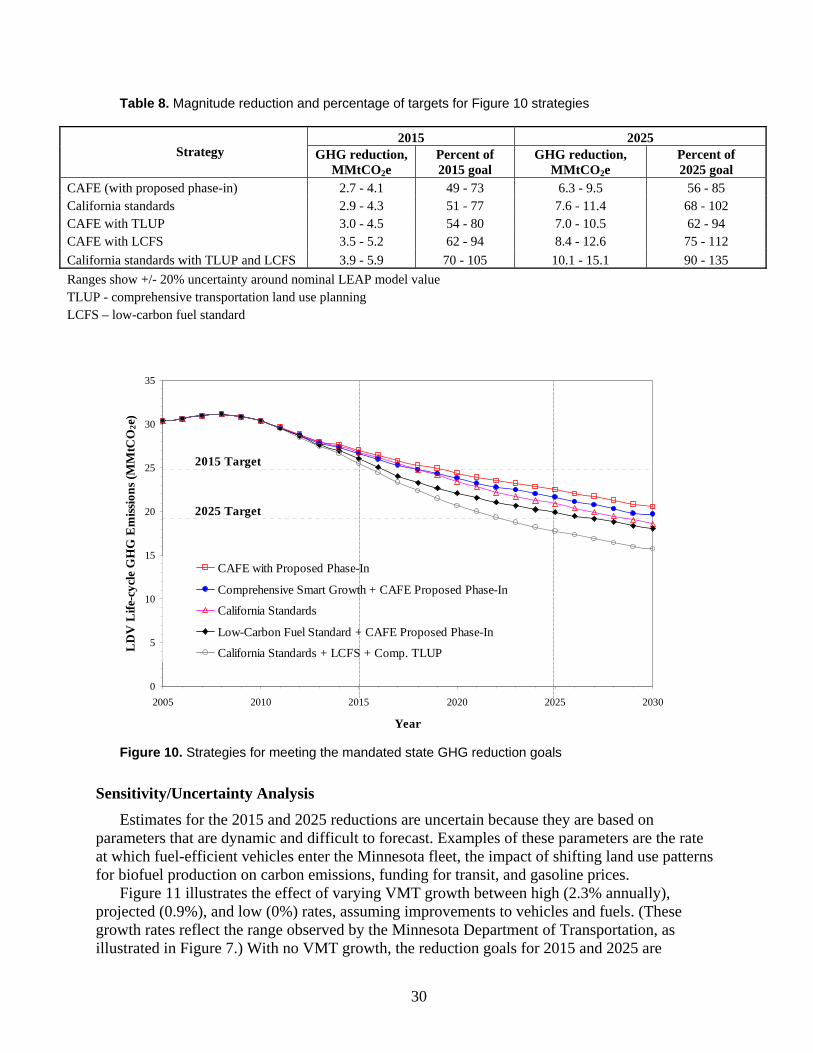
30

Table 8. Magnitude reduction and percentage of targets for Figure 10 strategies

2015 2025 Strategy GHG reduction,

MMtCO2e Percent of 2015 goal

GHG reduction, MMtCO2e

Percent of 2025 goal

CAFE (with proposed phase-in) 2.7 - 4.1 49 - 73 6.3 - 9.5 56 - 85 California standards 2.9 - 4.3 51 - 77 7.6 - 11.4 68 - 102 CAFE with TLUP 3.0 - 4.5 54 - 80 7.0 - 10.5 62 - 94 CAFE with LCFS 3.5 - 5.2 62 - 94 8.4 - 12.6 75 - 112 California standards with TLUP and LCFS 3.9 - 5.9 70 - 105 10.1 - 15.1 90 - 135 Ranges show +/- 20% uncertainty around nominal LEAP model value TLUP - comprehensive transportation land use planning LCFS – low-carbon fuel standard

0

5

10

15

20

25

30

35

2005 2010 2015 2020 2025 2030

Year

LD

V L

ife-c

ycle

GH

G E

miss

ions

(MM

tCO

2e)

CAFE with Proposed Phase-In

Comprehensive Smart Growth + CAFE Proposed Phase-In

California Standards

Low-Carbon Fuel Standard + CAFE Proposed Phase-In

California Standards + LCFS + Comp. TLUP

2015 Target

2025 Target

Figure 10. Strategies for meeting the mandated state GHG reduction goals

Sensitivity/Uncertainty Analysis Estimates for the 2015 and 2025 reductions are uncertain because they are based on

parameters that are dynamic and difficult to forecast. Examples of these parameters are the rate at which fuel-efficient vehicles enter the Minnesota fleet, the impact of shifting land use patterns for biofuel production on carbon emissions, funding for transit, and gasoline prices.

Figure 11 illustrates the effect of varying VMT growth between high (2.3% annually), projected (0.9%), and low (0%) rates, assuming improvements to vehicles and fuels. (These growth rates reflect the range observed by the Minnesota Department of Transportation, as illustrated in Figure 7.) With no VMT growth, the reduction goals for 2015 and 2025 are

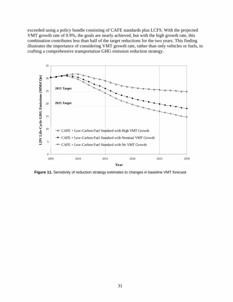
31

exceeded using a policy bundle consisting of CAFE standards plus LCFS. With the projected VMT growth rate of 0.9%, the goals are nearly achieved, but with the high growth rate, this combination contributes less than half of the target reductions for the two years. This finding illustrates the importance of considering VMT growth rate, rather than only vehicles or fuels, in crafting a comprehensive transportation GHG emission reduction strategy.

0

5

10

15

20

25

30

35

2005 2010 2015 2020 2025 2030

Year

LDV

Life

-Cyc

le G

HG

Em

issi

ons (

MM

tCO 2

e)

CAFE + Low-Carbon Fuel Standard with High VMT Growth

CAFE + Low-Carbon Fuel Standard with Nominal VMT Growth

CAFE + Low-Carbon Fuel Standard with No VMT Growth

2015 Target

2025 Target

Figure 11. Sensitivity of reduction strategy estimates to changes in baseline VMT forecast

32

33

CHAPTER 5: PROMISING TECHNOLOGIES AND STRATEGIES FOR ACHIEVING 2050 GOALS

Estimating transportation GHG emissions in 2050 would be highly speculative, as federal

and state agencies do not provide forecasts of parameters needed for modeling GHG emissions that far in the future. Because of this, we discuss the year–2050 GHG reduction goal (80% relative to 2005) qualitatively rather than quantitatively. Specifically, we discuss adoption of technologies and strategies that show promise to ensure the state is in a position to meet the 2050 reduction target. Many of the technologies and strategies below have been initiated, but some issues remain.

Hybrid Vehicles A potentially significant GHG-reducing technology that is already available is the hybrid

electric vehicle (HEV). HEVs combine a conventional gasoline or diesel propulsion system with an on-board, rechargeable energy storage system to achieve better fuel economy without loss of vehicle range. HEVs obtain all of their energy from liquid fuel, and obtain no energy from plug-in electricity; the key difference compared to a conventional vehicle is that the HEV engine is more efficient. Examples of this technology now on the road are the Honda Civic, Toyota Prius, and Ford Escape.

A modification to HEVs—not yet available in widespread production but undergoing research and development—is the plug-in hybrid electric vehicle (PHEV). The PHEV is a hybrid vehicle with batteries that can be recharged by connecting a plug to an electric power source. Compared to a conventional vehicle, the maximum per vehicle fuel reduction expected from an HEV is about 30%, and 45% or more from a PHEV (Simpson, 2006).

Although the PHEV shows great promise, the degree to which PHEV technology can reduce GHG emissions depends on four key factors:

• The distance vehicles can drive between charging. The greater the distance, the less conventional fuel consumed.

• The infrastructure for charging, which determines where and when a vehicle can be charged

• The GHG footprint of the electricity used to recharge the vehicles • The cost of the PHEV

The life-cycle GHG footprint of the electricity source determines the degree of GHG reduction. As the electrical sector continues to reduce GHG emissions, life-cycle emissions associated with driving PHEVs will correspondingly decrease without further vehicle modifications. Low-carbon electricity may come from a variety of sources including wind, solar, biomass, hydro, nuclear, and fossil fuels with carbon capture and storage. Of relevance to Minnesota is a recent study that shows direct usage of cellulosic biomass (i.e., burning it) to produce electricity provides a greater GHG reduction than when the same cellulosic biomass is refined to liquid fuel (Eickhout, et al., 2008). In this instance, no new technology to utilize the biomass is required.

If PHEVs become widespread, life-cycle emissions from electricity will affect the transportation sector’s ability to meet 2050 GHG reduction targets. At present, the high GHG emissions from electricity consumed in Minnesota—attributable mainly to the large proportion

34

of coal-based electricity—significantly reduce the GHG benefits from PHEVs. Charging should be synchronized with low electrical usage and with periods when power is produced from cleaner sources such as nuclear, natural gas, or wind. During the off-peak electrical generation hours, the vast majority of Minnesota’s electricity is produced by coal and nuclear, because these plants are seldom shut down and are therefore constantly producing electricity. Electricity from coal has high GHG emissions—0.95 g/Wh—compared with other sources of energy such as natural gas, at 0.50 g/Wh (Jaramillo, et al. 2007). Charging PHEVs with electricity produced by conventional coal power plants may actually increase GHG emissions compared to the HEV.

Emission reductions could come from steps such as switching away from coal or from carbon capture and storage. Fuel switching is a currently available option; carbon capture and storage is in the early stages of research and development but may become important for meeting targets after 2025.

Infrastructure Another important step toward positioning the state for meeting the 2050 targets is to develop

infrastructure to shift the long-distance transport of freight and passengers to more energy-efficient modes such as rail. This mode shift requires a substantial commitment by policymakers to invest in infrastructure improvements over the long term—but the GHG reduction benefits may be substantial. Trains, for example, move freight at a rate of 202 ton-miles per gallon, compared with trucks at a rate of 59 ton-miles per gallon (Grier, 2002). All other parameters being equal, the GHG gas reduction for each ton-mile of freight shifted from trucks to trains is almost a factor of 4.

Fuels For travel beyond the range of electric vehicles but not within the network of railways, liquid

fuel options must be developed to deliver higher-energy density with lower associated emissions. The creation of cellulosic ethanol from prairie grasses for use in conventional vehicles is a strategy that shows potential in this area and should be explored.

A diesel fuel/engine technology that shows promise is dimethyl ether (DME). The production of DME from biomass promises higher efficiencies and lower associated emissions than direct synthesis of synthetic diesel fuel derived from biomass (Semelsberger, et al. 2006). DME use in diesel engines increases engine efficiency by allowing engines to be tuned to higher efficiencies without the production of black carbon, which is a major cause of global warming (Jacobson, 2007). While prototype DME buses exist in China and Denmark and DME trucks are in development in Sweden and Japan, further study is needed to determine how DME can be integrated into the Minnesota fleet (Hansen, et al., 2001; Williams, et al., 2003).

Land Use and System Shifts Land use and system shifts of passenger and vehicle miles to other modes of transportation

exhibit a promising means for long-term emissions reductions from the transportation sector. The development of public transit and complementary land uses provides short- and mid-term GHG reductions while also providing a framework for future reductions.

Zurich, Switzerland, provides an example of the impact of coordinating the public transportation system and land use planning. More than a third of middle-income families in Zurich

35

do not own cars and rely on a combination of car-sharing and public transportation, even though the city has one of the highest standards of living in the world. In addition to the reduction of GHG emissions, there are a number of co-benefits as well, such as land and resource conservation, air pollution benefits, and equity of access to transportation by young and old citizens (Cervero 1998, 2001).

Reported and projected transit system ridership in Minnesota demonstrates the substantial reductions in GHG emissions that vehicle mode shifts can make. Current Metro Transit buses in the Twin Cities produce 16% less GHG emissions per passenger-mile relative to personal vehicles. Commuter and light rail can yield GHG reductions of 40% and 75%, respectively, while choosing rail rather than air for long-range passenger travel reduces emissions by up to 28%.

Similar results have been found for long-distance freight transport. A 2002 study of freight transport in Australia found that combination rail/truck transport of freight had only 31% to 70% of the emissions associated with transport by truck alone (QR Network Access, 2002). An increased electrification of freight and passenger transport is also likely. As with PHEVs, the benefits associated with electrified freight transport vehicles will depend on the life-cycle greenhouse emissions of the electric power used.

36

37

CHAPTER 6: CONCLUSIONS Our study shows that Minnesota’s 2015 and 2025 reduction goals are technologically

achievable. The goals are nearly met in 2015 and are exceeded in 2025 using a combination of strategies targeted to reduce fuel consumption, vehicle-miles traveled, and fuel carbon content for the light-duty vehicle fleet.

Other conclusions:

• Vehicle technology available now or in the short term supports efficiency standards considerably more aggressive than those being considered for U.S. implementation. These would produce correspondingly greater GHG reductions from the light-duty vehicle fleet.

• Vehicle and fuel policies such as the low-carbon fuel standard and California emissions standards are most effective when implemented across a broad base that includes other states.

• Well-to-wheel (or field-to-wheel) life-cycle analysis is necessary to estimate GHG emissions from the transportation sector. This analysis is affected by cross-cutting issues such as methods used to generate electricity, assumptions used to estimate reductions, and the modeling method.

• Although this report does not comprehensively address the economic impact of GHG reduction strategies, we have shown that requiring higher-efficiency vehicles—for example, ones complying with the California standards—yields a net cost savings to the consumer, because the savings produced by the increased fuel economy more than offset the cost of the technology. California has also shown that there would be a net benefit to the California economy should the standards be adopted.

• GHG-reduction strategies must include attention to VMT. Otherwise, improvements in vehicles and fuels may be largely offset by VMT increases.

38

39

REFERENCES An, F., and A. Sauer. 2004. Comparison of Passenger Vehicle Fuel Economy and

Greenhouse Gas Emission Standards Around the World. Arlington,VA: Pew Center on Global Climate Change. (www.pewclimate.org/docUploads/Fuel%20Economy%20and%20GHG%20Standards_010605_110719.pdf.)

An, F., D. Gordon, H. He, D. Kodjak, and D. Rutherford. 2007. Passenger Vehicle

Greenhouse Gas and Fuel Economy Standards: A Global Update. International Council on Clean Transportation (http://www.theicct.org/documents/ICCT_GlobalStandards_20071.pdf)

Ang-Olson, J., and W. Schroeer. 2002. Energy efficiency strategies for freight trucking:

potential impact on fuel use and greenhouse gas emissions. Transportation Research Record, 1815:11-18. Washington, DC: Transportation Research Board. (http://trb.metapress.com/content/57024v26279332n5/)

Brandt, A.R., and A.E. Farrell. 2007. Scraping the bottom of the barrel: greenhouse gas

emission consequences of a transition to low-quality and synthetic petroleum resources. Climate Change, 84:241-263.

Bureau of Transportation Statistics. 2006a. State Transportation Statistics 2006. U.S.

Department of Transportation, Research and Innovative Technology Administration. (http://www.bts.gov/publications/state_transportation_statistics/state_transportation_statistics_2006/index.html).

Bureau of Transportation Statistics. 2006. Table 1-32: U.S. Vehicle-Miles.

(http://www.bts.gov/publications/national_transportation_statistics/html/table_01_32.html) California Air Resources Board. 2005. Regulations to Control Greenhouse Gas Emissions

from Motor Vehicles: Final Statement of Reasons. California Environmental Protection Agency Air Resources Board, Aug. 4, 2005. (http://www.arb.ca.gov/regact/grnhsgas/grnhsgas.htm)

California Air Resources Board. 2008a. Comparison of Greenhouse Gas Reductions for the

United States and Canada Under U.S. CAFE Standards and California Air Resources Board Greenhouse Gas Regulations (An Enhanced Technical Assessment). California Air Resources Board. (http://www.arb.ca.gov/cc/ccms/ccms.htm)

California Air Resources Board. 2008b. Addendum to February 25 Technical Assessment.

Comparison of Greenhouse Gas Reductions for the United States and Canada Under ARB GHG Regulations and Proposed Federal 2011-2015 Model Year Fuel Economy Standards. (http://www.arb.ca.gov/cc/ccms/reports/final_pavleyaddendum.pdf)

40

California Attorney General's Office. 2007. A Comparison of California GHG Standards and the Senate Cafe Target. (http://ag.ca.gov/cms_attachments/press/pdfs/n1493_energybill_attachment.pdf)

California Energy Commission. 2003. Reducing Petroleum Dependency in California. Staff

Paper on Option 3B Feebates (Appendix C (revised), Attachment B). (http://www.energy.ca.gov/fuels/petroleum_dependence/documents/)

Center for Clean Air Policy (CCAP). 2006. CCAP Transportation Emissions Guidebook -

Part Two: Vehicle Technology and Fuels. (http://www.ccap.org/domestic/smart.htm) Center for Climate Strategies. 2008. Final Minnesota Greenhouse Gas Inventory and

Reference Case Projections, 1990–2025. Prepared for the Minnesota Pollution Control Agency, February 2008. http://www.mnclimatechange.us/ewebeditpro/items/O3F16231.pdf

Cervero, R. 1998. The Transit Metropolis: A Global Inquiry. Washington, DC: Island Press. Cervero, R. 2001. Transport and land use: key issues in metropolitan planning and smart

growth. Australian Planner, Vol. 38, No. 1, 1-23. (http://www.uctc.net/papers/436.pdf) Delucchi, M. A. 2006. Lifecycle Analysis of Biofuels. Draft Report. UC Davis report UCD-

ITS-RR-06-08. (http://www.its.ucdavis.edu/publications/2006/UCD-ITS-RR-06-08.pdf) Dierkers, G., E. E. Silsbe, S. Stott, S. Winkelman, and M. Wubben. 2007. CCAP

Transportation Emissions Guidebook, Part One: Land Use, Transit & Travel Demand Management. Washington DC: Center for Clean Air Policy. (http://www.trb.org/news/blurb_detail.asp?id=5294)

Doughman, P. M. 2007. California's climate change policy. Environment, Vol. 49, No. 7, 10. Edwards, R., J.-F. Larivé, V. Mahieu, and P. Rouveirolles. 2007. Well-to-Wheels Analysis of

Future Automotive Fuels and Powertrains in the European Context: Well-to-Wheels Report, EUCAR, CONCAWE and JRC/IES. 2B. (http://www.eucar.be/start.html)

Eickhout, B., G. J. van den Born, J. Notenboom, M. van Oorschot, J.P.M. Ros, D.P. van

Vuuren, and H.J. Westhoek. 2008. Local and global consequences of the EU renewable directive for biofuels. Amsterdam: Netherlands Environmental Assessment Agency. (http://www.mnp.nl/en/publications/2008/LocalandglobalconsequencesoftheEUrenewabledirectiveforbiofuels.html)

Ellerman, D.A., H.D. Jacoby, and M.B. Zimmerman. 2006. Bringing Transportation Into a

Cap-and-Trade Regime. Cambridge, MA: MIT Joint Program on the Science and Policy of Global Change, Report 136. (http://mit.edu/globalchange/www/MITJPSPGC_Rpt136.pdf)

41

Energy Information Agency. 2007. Supplemental Tables to the Annual Energy Outlook 2007, Table 49 - Light Duty Vehicle MPG by Technology Type. U.S. Department of Energy. (http://www.eia.doe.gov/oiaf/aeo/supplement/)

Energy Information Agency. 2008. Table 18 Carbon Dioxide Emissions by Sector and

Source. U.S. Department of Energy. (http://www.eia.doe.gov/oiaf/aeo/excel/aeotab_18.xls) Environmental Protection Agency. 2008a. Clean Air Act.

(http://www.epa.gov/air/caa/caa209.txt http://www.epa.gov/air/caa/caa177.txt http://www.epa.gov/air/caa/) Environmental Protection Agency. 2008b. Smartway Transport Partnership - Partners -

Minnesota. (http://epa.gov/smartway/partners/minnesota-trucking-association.htm) Ewing, R., K.Bartholomew, S. Winkelman, J.Walters, and D. Chen. 2007. Growing Cooler:

The Evidence on Urban Development and Climate Change. Urban Land Institute and Smart Growth America. (http://www.smartgrowthamerica.org/gcindex.html)

Fargione, J., J. Hill, D. Tilman, S. Polasky, and P. Hawthorne. 2008. Land clearing and the

biofuel carbon debt. Science, Vol. 319, No. 5867, pp. 1235-1238. (http://www.sciencemag.org/cgi/reprint/319/5867/1235.pdf)

Farrell, A., and D. Sperling. 2007a. A Low-Carbon Fuel Standard for California-Part 1:

Technical Analysis. University of California-Berkeley. (http://repositories.cdlib.org/its/tsrc/UCB-ITS-TSRC-RR-2007-2/)

Farrell, A., and D. Sperling. 2007b. A Low-Carbon Fuel Standard for California Part 2:

Policy Analysis. University of California-Berkeley. (http://repositories.cdlib.org/its/tsrc/UCB-ITS-TSRC-RR-2007-3/)

Fournier, A. 2006. Controlling air emissions from marine vessels: problems and

opportunities. Environmental Science and Management. Santa Barbara: University of California at Santa Barbara. (http://www.westcoastcollaborative.org/files/sector-marine/Fournier%20Marine%20Emissions%20Problems%20and%20Opportunities.pdf)

Grier, D. V. 2002. Comparison of inland waterways and surface freight modes. TR News.

Transportation Research Board, No. 221, July-August 2002. (http://onlinepubs.trb.org/onlinepubs/trnews/trnews221.pdf)

Greene, D. L., P. D. Patterson, M. Singh, and J. Li. 2005. Feebates, rebates and gas-guzzler

taxes: a study of incentives for increased fuel economy. Energy Policy, Vol. 33, No. 6, 757-775. Hansen, J. B., and S. E. Mikkelsen. 2001. DME as a Transportation Fuel. Lyngby, Denmark:

The Danish Road Safety and Transportation Agency & The Danish Environmental Protection Agency. (http://www.trm.dk/graphics/synkron-library/faerdselsstyrelsen/dokumenter/publikation/Publikationer/dme_eng.pdf)

42

Heaps, C. 2008. Long Range Energy Alternatives Planning System: An Introduction to

LEAP. (http://www.energycommunity.org/documents/LEAPIntro.pdf) Jacobson, M. Z. 2007. Testimony for the Hearing on Black Carbon and Global Warming,

House Committee on Oversight and Government Reform, United States House of Representatives. Oct 18, 2007. Washington, D.C.: Government Printing Office, 2007. (http://www.stanford.edu/group/efmh/jacobson/0710LetHouseBC1.pdf)

Jaramillo, P., W. M. Griffin, and H.S. Matthews. 2007. Comparative life-cycle air emissions

of coal, domestic natural gas, LNG, and SNG for electricity generation. Environmental Science & Technology, Vol. 41, No. 17, 6290-6296.

Lal, R. 2005. World crop residues production and implications of its use as a biofuel.

Environment International, Vol. 31, No. 4, 575-584. Levine, J. 2006. Zoned out: regulation, markets, and choices. Transportation and

Metropolitan Land Use. Washington, D.C.: RFF Press. Marshall, J., T., E. McKone, E. Deakind, and W. W. Nazaroff. 2005. Inhalation of motor

vehicle emissions: effects of urban population and land area. Atmospheric Environment, 39: 283-295.

Marshall, J.D. 2008. Energy-efficient urban form. Environmental Science & Technology,

42(9), pp. 3133-3137. McManus, W. S. 2007. Economic Analysis of Feebates to Reduce Greenhouse Gas

Emissions from Light Vehicles for California. University of Michigan-Ann Arbor: Transportation Research Institute, 9 pp. (http://www.umtri.umich.edu/content/UMTRI-2007-19-1.pdf)

Metropolitan Council. 2007. Hiawatha Light-Rail Transit Fact Sheet.

(http://www.metrocouncil.org/about/facts/HiawathaLRTFacts.pdf) Metropolitan Council. 2000. 2000 Travel Behavior Inventory: Home Interview Survey Data

and Methodology. (http://www.metrocouncil.org/planning/transportation/TBI_2000.htm) Metropolitan Transit. (2007). Facts About Trains and Construction.

(http://www.metrotransit.org/rail/facts.asp.) Minnesota Climate Change Advisory Group, 2008. Report to the Minnesota Legislature.

April, 2008. http://www.mnclimatechange.us/MCCAG.cfm Minnesota Department of Transportation. 2005. Daily (Average) and Annual (Total) Vehicle

Miles --- 2005 Grouped by Route System for Each County (http://www.dot.state.mn.us/roadway/data/reports/2005/vmt/fzstvmig.pdf)

43

Minnesota Department of Transportation. 2008. Statewide Transportation Plan Update:

Setting the Context - Key Trends and Indicators. Statewide Transportation Steering Committee. (http://www.oim.dot.state.mn.us/STP/pdfs/Legislative%20Staff%20Briefing.pdf)

Minnesota Pollution Control Agency. 2007. UMCTS (Minnesota GHG Emissions and Other

Transportation Indicators 1970-2004). Personnel communication, Aug 3, 2007 to P. S. Nussbaum from P. Ciborowski.

Minnesota Pollution Control Agency. 2008. Ethanol Facilities in Minnesota — Present and

Future. January 25, 2008. (http://www.pca.state.mn.us/publications/ethanol-sitemap.pdf) Minnesota Senate. 2007. Next Generation Energy Act of 2007, S.F. No. 145, 2nd

Engrossment—85th Legislative Session (2007–2008). May 21, 2007. (https://www.revisor.leg.state.mn.us/bin/bldbill.php?bill=S0145.2.html&session=ls85

Mui, S., J. Alson, B. Ellies, and D. Gauss. 2007. A Wedge Analysis of the U.S.

Transportation Sector. Environmental Protection Agency. EPA 420-R-07-007, 23 pp. National Highway Traffic Safety Administration. 2008. Average Fuel Economy Standards

Passenger Cars and Light Trucks Model Years 2011-2015. Department of Transportation. 49 CFR Parts 523, 531, 533, 534, 536 and 537. (http://www.nhtsa.dot.gov/staticfiles/DOT/NHTSA/Rulemaking/Rules/Associated%20Files/CAFE_11-15_NPRM_April_21.pdf)

QR Network Access. 2002. Comparison of Greenhouse Gas Emissions by Australian

Intermodal Rail and Road Transport. Brisbane: Affleck Consulting Pty Ltd. (http://www.networkaccess.qr.com.au/Images/Emissions_tcm10-2847.pdf)

Schwarzenegger, A. 2007. Low Carbon Fuel Standard Program. State of California,

Executive Order S-01-07, Jan 18, 2007. (http://gov.ca.gov/executive-order/5172/) Searchinger, T., R. Heimlich, R. A. Houghton, F. Dong, A. Elobeid, J. Fabiosa, S. Tokgoz,

D. Hayes, and T.-H. Yu. 2008. Use of U.S. croplands for biofuels increases greenhouse gases through emissions from land use changes. Science, Vol. 319, No. 5867, 1238-1240. (http://www.sciencemag.org/cgi/content/abstract/1151861)

Semelsberger, T. A., R. L. Borup, and H.L. Greene. 2006. Dimethyl ether (DME) as an

alternative fuel. Journal of Power Sources, Vol. 156, No. 2, 497-511. Simpson, A. 2006. Cost-Benefit Analysis of Plug-In Hybrid Electric Vehicle Technology.

U.S. Department of Energy. National Renewable Energy Laboratory. (http://www.nrel.gov/vehiclesandfuels/vsa/pdfs/40485.pdf)

44

Smart Growth America. 2002. Measuring Sprawl and Its Impact: The Character and Consequences of Metropolitan Expansion. (http://www.smartgrowthamerica.org/sprawlindex/sprawlindex.html)

Socolow, R., and S. Pacala. 2004. Stabilization wedges: solving the climate problem for the

next 50 years with current technologies. Science, Vol. 305, 968-972. State of Nebraska. 2008. Ethanol Production by State. Retrieved Mar 30, 2008 from

http://www.neo.ne.gov/statshtml/121.htm. Subin, Z. 2007. GHG Abatement Supply Curves for California's Transportation Sector

Working Paper. UC-Berkeley Energy & Resources Group Energy & Environmental Economics, December 21, 2007, 67 pp. (http://captainjack74737.fastmail.fm/CA_Transp_GHG_Opt_WP_12_07.pdf)

U.S. Census Bureau. 2007. (http://www.census.gov/popest/states/tables/NST-EST2007-

01.xls) U.S. Department of Transportation. 1995a. State Motor-Vehicle Registration 2005.

(http://www.fhwa.dot.gov/ohim/1995/mv1.pdf) U.S. Department of Transportation. 1995b. Annual Vehicle-Miles of Travel – 1995 By

Functional System. (http://www.fhwa.dot.gov/ohim/1995/vm2.pdf) U.S. Department of Transportation. 2005a. State Motor-Vehicle Registration 2005.

(http://www.fhwa.dot.gov/policy/ohim/hs05/pdf/mv1.pdf) U.S. Department of Transportation. 2005b. Highway Statistics 2005 Selected Measures for

Identifying Peer States (http://www.fhwa.dot.gov/policy/ohim/hs05/htm/ps1.htm) Vasic, B. 2008. As gas costs soar, buyers are flocking to small cars. New York Times, May 2,

2008, page A1. Wald, M. L. 2008. E.P.A. chief defends his decision on California. New York Times. Jan 25,

2008. (http://www.nytimes.com/2008/01/25/washington/25environ.html) Wang, M., 1999. Transportation Fuel-Cycle Model, Volume 1: Methodology, Development,

Use, and Results. Center for Transportation Research, Energy Systems Division, Argonne National Laboratory. (http://www.osti.gov/bridge/product.biblio.jsp?osti_id=14775)

Williams, R. H., and E. D. Larson 2003. A comparison of direct and indirect liquefaction

technologies for making fluid fuels from coal. Energy and Sustainable Development, Vol. 7, No. 4, 103-129.