Reference Governor for Constrained Piecewise Affine

Systems

Francesco Borrellia,∗, Paolo Falconeb, Jaroslav Pekarc, Greg Stewartd

aDepartment of Mechanical Engineering, University of California, Berkeley, 94720-1740,

USAbDepartment of Signals and Systems, Chalmers University of Technology, Goteborg,

SE-412 96, SwedencHoneywell Prague Laboratory, Honeywell Intl., Pod voda renskou, vezı 4, 182 04 Prague

8, Czech RepublicdHoneywell Automation and Control Solutions, North Vancouver, BC V7J 3S4, Canada

Abstract

We present a methodology for designing reference tracking controllers forconstrained, discrete-time piecewise affine systems. The approach follows theidea of reference governor techniques where the desired set-point is filtered bya system called the “reference governor”. Based on the system current state,set-point, and prescribed constraints, the reference governor computes a newset-point for a low-level controller so that the state and input constraints aresatisfied and convergence to the original set-point is guaranteed.

In this note we show how to design a reference governor for constrainedpiecewise affine systems by using polyhedral invariant sets, reachable sets,multiparametric programming and dynamic programming techniques.

Key words: Model Predictive Control, Process Control

1. Introduction

Different methods for the analysis and design of controllers for hybridsystems have emerged in the past [39, 31, 4]. Among them, the class of

∗Corresponding authorEmail addresses: fborrelli@me.berkeley.edu (Francesco Borrelli),

falcone@chalmers.se (Paolo Falcone), Jaroslav.Pekar@Honeywell.com (JaroslavPekar), greg.stewart@honeywell.com (Greg Stewart)

Preprint submitted to International Journal of Process Control June 15, 2009

optimal controllers is one of the most studied. The existing approaches differgreatly in the hybrid models adopted, in the formulation of the optimalcontrol problem and in the method used to solve it. In this work we willfocus on discrete-time piecewise affine (PWA) models. Discrete-time PWAmodels can describe a large number of processes, such as: discrete-time linearsystems with static piecewise-linearities; discrete-time linear systems withdiscrete states and inputs; switching systems where the dynamic behavior isdescribed by a finite number of discrete-time linear models together with a setof logic rules for switching among these models; approximation of nonlineardiscrete-time dynamics, e.g., via multiple linearizations at different operatingpoints.

This work deals with the design of reference-tracking state-feedback con-trollers for constrained PWA systems. Our interest stems from industrialpractice where, for control synthesis purposes, nonlinear plants are often ap-proximated by partitioning the space spanned by the inputs, state, and ex-ogenous signals into a finite number of regions (also called “modes”). Eachregion is then assigned an affine model and the nonlinear system is thus ap-proximated by a PWA system. A standard gain scheduling strategy consistsof designing a linear controller for each region along with an appropriatestrategy for switching between them. It should be noted that the resultingclosed-loop system contains reference signals for the controller which are ex-ogenous to the closed-loop. In order to satisfy the state and input constraints,the control designer has to explicitly consider the case where a change in thereference signal results in a system transition between two or more regions.

In principle one could solve an optimal tracking problem for the con-strained PWA systems by using the approach presented in [15]. There theauthors have characterized the state-feedback solution to optimal controlproblems for PWA systems with performance criteria based on quadratic andlinear norms. They have shown that the solution is a time-varying piecewiseaffine feedback control law, possibly defined over non-convex regions andproposed an algorithm that solves the Hamilton-Jacobi-Bellman equation byusing a simple multiparametric solver. However, the implementation of theexplicit controller might require significant computation infrastructure whichmight not be available on processes with fast sampling time and limited com-putational resources.

In order to overcome this limitation, one possibility is to design lowcomplexity suboptimal constrained controllers as proposed in [24]. In thispaper we present an approach based on the concept of “reference gover-

2

nor” [6, 7, 8, 3, 2, 40, 29, 21, 22]. The idea underlying reference governor isto add a nonlinear device to a controlled system. Such device is called refer-ence governor (RG) and its operation is based on the current state, set-point,and prescribed constraints. Typically the RG selects at any time a virtualreference sequence among a family of linearly parameterized sequences, bysolving a convex constrained quadratic optimization problem, and feeds thecontrolled system according to a receding horizon control philosophy [6]. Theoverall system is proved to fulfill the constraints, be asymptotically stable,and exhibit an offset-free tracking behavior, provided that an admissibilitycondition on the initial state is satisfied [6].

This work shows how to design a reference governor for constrainedpiecewise-affine systems by using polyhedral invariant sets, reachable sets,multiparametric programming and dynamic programming. Compared to theinfinite time optimal solution [15, 14] the approach presented in this paperwill be less computationally demanding at the price of suboptimality and asmaller region of attraction. In particular our approach can lead to empty orsmall feasibility regions and it will not succeed if the PWA system cannot bestabilized in any mode (e.g. stability can only be obtained by continuouslyswitching between modes).

We remark that there exist other other very efficient approaches appearedin the literature for solving optimal control problems for PWA systems [25,1, 11, 38, 18]. The comparison would be problem dependent and requires thesimultaneous analysis of several issues such as speed of computation, storagedemand and real time code verifiability. This is an involved study and assuch is outside of the scope of this paper.

The paper is organized as follows. We give a short overview on multi-parametric programming and on invariant sets in Section 2. The formulationof reference-tracking state-feedback controllers for constrained PWA systemsis presented in Section 3. In Section 4 we introduce and discuss the referencegovernor algorithm. Finally, in Section 5 an example is given that confirmsthe efficiency of the new method.

2. Definitions and Basic Results

In this section we introduce a few definitions and then recall some basic re-sults on multi-parametric programming and invariant set theory. We willdenote the set of all real numbers and positive integers by R and N

+, respec-tively.

3

Definition 1. A polyhedron is a set that equals the intersection of a finitenumber of closed halfspaces.

Definition 2. A collection of sets R1, . . ., RN is a partition of a set Θ if(i)

⋃N

i=1 Ri = Θ, (ii) Ri ∩ Rj = ∅, ∀i 6= j. Moreover R1, . . ., RN is apolyhedral partition of a polyhedral set Θ if R1, . . ., RN is a partition of Θand the Ri’s are polyhedral sets, where Ri denotes the closure of the set Ri.

Definition 3. A function h : Θ → Rk, where Θ ⊆ R

s, is piecewise affine(PWA) if there exists a partition R1,. . . ,RN of Θ and h(θ) = H iθ + ki,∀θ ∈ Ri, i = 1, . . . , N .

Definition 4. A function h : Θ → Rk, where Θ ⊆ R

s, is PWA on polyhedra(PPWA) if there exists a polyhedral partition R1,. . . ,RN of Θ and h(θ) =H iθ + ki, ∀θ ∈ Ri, i = 1, . . . , N .

Piecewise quadratic functions (PWQ) and piecewise quadratic functions onpolyhedra (PPWQ) are defined analogously.

2.1. Background on Multiparametric programming

Consider the nonlinear mathematical program dependent on a parametervector θ appearing in the cost function and in the constraints

J∗(θ) = infz

J(z, θ)

subj. to g(z, θ) ≤ 0z ∈M,

(1)

where z ∈ Rs is the optimization vector, θ ∈ R

n is the parameter vector,J : R

s × Rn → R is the cost function, g : R

s × Rn → R

ng are the constraintsand M ⊆ R

s. A small perturbation of the parameter θ in (1) can cause avariety of outcomes, i.e., depending on the properties of the functions J andg the solution z∗(θ) may vary smoothly or change abruptly as a function ofθ. We denote by K∗ the set of feasible parameters, i.e.,

K∗ = {θ ∈ Rn | ∃z ∈ M, g(z, θ) ≤ 0}, (2)

by R : Rn → 2R

s

, where 2Rs

denotes the set of all subsets of Rs, the point-

to-set map that assigns the set of feasible z

R(θ) = {z ∈M | g(z, θ) ≤ 0} (3)

4

to a parameter θ, by J∗ : K∗ → R ∪ {−∞} the real-valued function whichexpresses the dependence on θ of the minimum value of the objective functionover K∗, i.e.

J∗(θ) = infz{J(z, θ) | θ ∈ K∗, z ∈ R(θ)}, (4)

and by Z∗ : K∗ → 2Rs

the point-to-set map which expresses the dependenceon θ of the set of optimizers, i.e, Z∗(θ) = {z ∈ R(θ) |J(z, θ) = J∗(θ)} withθ ∈ K∗.

J∗(θ) will be referred to as the optimal value function or simply valuefunction, Z∗(θ) will be referred to as the optimal set. We will denote byz∗ : R

n → Rs one of the possible single valued functions that can be extracted

from Z∗, z∗ will be called the optimizer function. If Z∗(θ) is a singleton forall θ, then z∗(θ) is the only element of Z∗(θ).

Optimal control problems for nonlinear systems can be reformulated asthe mathematical program (1) where z is the input sequence to be optimizedand θ the initial state of the system. Therefore, the study of the propertiesof J∗ and Z∗ is fundamental for the study of properties of state-feedback op-timal controllers. Fiacco ([19, Chapter 2]) provides conditions under whichthe solution of nonlinear multiparametric programs (1) is locally well behavedand establishes properties of the solution as a function of the parameters. Inthis note we restrict our attention to the following special class of multipara-metric programming:

J∗(θ) = 12θ′Y θ + min

z

12z′Hz + z′Fθ

subj. to Cz ≤ c+ Sθ(5)

where z ∈ Rs is the optimization vector, θ ∈ R

n is the vector of parameters,and C ∈ R

nc×s, c ∈ Rnc , S ∈ R

nc×n are constant matrices. We refer tothe problem of computing z∗(θ) and J∗(θ) in (5) as (right-hand-side) multi-parametric quadratic program (mp-QP).

Theorem 1 ([5]). Consider the mp-QP (5). Assume H ≻ 0 and [ Y F ′

F H ] � 0.The set K∗ is a polyhedral set, the value function J∗ : K∗ → R is PPWQ,convex and continuous and the optimizer z∗ : K∗ → R

s is PPWA and con-tinuous.

2.2. Background on Invariant Sets

This section adopts the notation used in [23, 37, 27] and provides thebasic definitions for invariant sets for constrained systems. A comprehensivesurvey of papers on set invariance theory can be found in [13].

5

Denote by fa the state update function of an autonomous system

x(t+ 1) = fa(x(t)) (6)

subject to the constraintsx(t) ∈ X (7)

For the autonomous system (6)-(7), we denote the set of states that evolvesto S in one step as

Prefa(S) , {x ∈ X | fa(x) ∈ S} (8)

Equivalently, for the system with inputs

x(t+ 1) = f(x(t), u(t)), (9)

subject to the constraints

x(t) ∈ X , u(t) ∈ U , (10)

the set of states which can be driven into the target set S in one time stepis defined as

Pref(S) , {x ∈ X | ∃u ∈ U s.t. f(x, u) ∈ S} (11)

Two different types of sets are considered in this note: invariant sets andcontrol invariant sets. We will first discuss invariant sets. The invariant setsare computed for autonomous systems and can be used to “find, for a givenfeedback controller u = k(x), the set of states whose trajectory will neverviolate the system constraints”. The following definitions are derived from[13, 10, 9, 28, 20].

Definition 5 (Positive Invariant Set). A set O is said to be a positiveinvariant set for the autonomous system (6) subject to the constraints in (7),if

x(0) ∈ O ⇒ x(t) ∈ O, ∀t ∈ N+

Control invariant sets are defined for systems subject to external inputs andcan be used to “find the set of states for which there exists a controller suchthat the system constraints are never violated”. The following definitions arederived from [13, 10, 9, 28].

6

Definition 6 (Control Invariant Set). A set C ⊆ X is said to be a con-trol invariant set for the system in (9) subject to the constraints in (10),if

x(t) ∈ C ⇒ ∃u(t) ∈ U such that f(x(t), u(t)) ∈ C, ∀t ∈ N+

For all states contained in the control invariant set there exists a controllaw, such that the system constraints are never violated. This does not implythat there exists a control law which can drive the state into a user-specifiedtarget set. This issue is addressed in the following by introducing the conceptof stabilizable sets.

Definition 7 (N-Step Stabilizable Set KN(f ;O)). For a given invarianttarget set O ⊆ X , the N-step stabilizable set KN(f ;O) of the system (9) sub-ject to the constraints (10) is defined as:

KN(f ;O) , Pref (KN−1(f ;O)), N ∈ N+

K0(f ;O) = O.

From Definition 7, all states x(0) belonging to the N -Step Stabilizable SetKN(f ;O) can be driven, through a time-varying control law, to the targetset O in N steps and stay in O for all t ≥ N while satisfying input and stateconstraints.

An equivalent definition can be given for the autonomous system (6)subject to the constraints in (7); all states x(0) belonging to the N -StepStabilizable Set KN (fa;O) will reach to the target set O in N steps and stayin O for all t ≥ N while satisfying state constraints.

3. Problem Formulation

Consider the PWA system

x(t+ 1) = Aix(t) +Biu(t) + ci

if[

x(t)u(t)

]

∈ P i, i = {1, . . . , s},(12)

where x ∈ Rn, u ∈ R

m, {P i}si=1 is a polyhedral partition of the set of the

state and input space P ⊂ Rn+m. The current index i will be called the

system mode, i.e., the PWA system (12) is in mode i at time t if[

x(t)u(t)

]

∈ P i.

7

System (12) is subject to hard input and state constraints

x(t) ∈ X , u(t) ∈ U (13)

for t ≥ 0, and we denote by Constrained PWA system (CPWA) the restrictionof the PWA system (12) over the set of states and inputs defined by (13),

x(t+ 1) = Aix(t) +Biu(t) + ci if[

x(t)u(t)

]

∈ P i, (14)

where {P i}si=1 is the new polyhedral partition of the sets of state and input

space Rn+m obtained by intersecting the sets P i in (12) with the polyhedron

described by (13). We assume the following.

Assumption 1. For a given reference state xref there is a unique inputuref = uref(xref) such that xref = Aixref +Biuref + ci if

[ xrefuref

]

∈ P i.The function uref(xref) is unique either from the properties of system (14)

(there is one mode and one uref for each xref) or by construction (i.e., forthe given xref the user specifies the desired mode and the corresponding uref).

Remark 1. Assumptions 1 is introduced for the sake of simplicity and itis not restrictive. It could be easily removed at the cost of a more complexnotation. In particular, if multiple equilibria are allowed, the best uref istypically chosen as a result of an optimization problem [35].

Our objective is to design a state feedback control law u(x, xref) suchthat the closed loop system

x(t+ 1) = Aix(t) +Biu(x(t), xref) + ci

if[

x(t)u(x(t),xref )

]

∈ P i,(15)

converges to xref and satisfies state and input constraints.A systematic approach to design constrained reference tracking controllers

is to use a receding horizon control policy. We define the following costfunction

JN(UN , x(0), xref) , ‖xN − xref‖2P

+∑N−1

k=0

[

‖xk − xref‖2Q + ‖uk − uref(xref)‖

2R

] (16)

8

with Q = Q′ � 0, R = R′ ≻ 0, P � 0, ‖x‖2M = x′Mx and consider the

constrained finite-time optimal control (CFTOC) problem

J∗

0 (x(0), xref) , minUNJ(UN , x(0), xref) (17)

subj. to

xk+1 = Aixk +Biuk + ci

if [ xkuk

] ∈ P i, i = 1, . . . , sxref,k+1 = xref,k

k = 0, . . . , N − 1

[xN , xref ] ∈ Xf

x0 = x(0), xref,0 = xref

(18)

where the column vector UN , [u′0, . . . , u′

N−1]′ ∈ R

mN , is the optimization

vector, N is the optimal control horizon. Xf is a polyhedral terminal regionin the [x, xref ]-space. Note that we distinguish between the input u(t) andthe state x(t) of plant (14) at time t and the variables uk and xk of theoptimization problem (18).

We will also denote by Xk ⊆ R2n the set of states xk and references xref

that are feasible for (16)-(18):

Xk =

x ∈ Rn,

xref ∈ Rn

∣

∣

∣

∣

∣

∣

∣

∣

∃u ∈ Rm,

∃i ∈ {1, . . . , s}[ xu ] ∈ P i and

[Aix+Biu+ ci, xref ] ∈ Xk+1

,

k = 0, . . . , N − 1,

XN = Xf .

(19)

Note that the optimizer function U∗

N may not be uniquely defined if theoptimal set of problem (16)-(18) is not a singleton for some x(0). The nexttheorem shows the properties of the optimal control solution.

Theorem 2 ([15]). Consider the optimal control problem (16)-(18). Then,there exists a solution in the form of a PWA state-feedback control law

u∗k(x(k), xref) = F x,ik x(k) + F u,i

k uref + F r,ik xref +Gi

k

if [x(k), xref ] ∈ Rik,

(20)

where Rik, i = 1, . . . , Nk is a partition of the set Xk of feasible states x(k)

and reference xref . The boundaries of the sets Rik are linear and quadratic

inequalities in x(k) and xref .

9

Note that quadratic inequalities in the sets Rik arise from the comparison

of quadratic costs associated to admissible switching sequences [15].An infinite horizon controller can be obtained by implementing in a re-

ceding horizon fashion a finite-time optimal control law. In this case thecontrol law is simply obtained by repeatedly evaluating at each time t thePWA controller (20) for k = 0:

u(t) = u∗0(x(t), xref) for[

x(t)xref

]

∈ X0. (21)

If Xf is a control invariant set and the terminal cost P is a control Lyapunovfunction, then for all [x(0), xref ] ∈ X0 the system state x(k) will convergeto the desired constant reference xref while satisfying input and state con-straints [33]. Note that the sets Xk are defined in the state and referencespace, since the initial state and the reference are both external parametersof the optimal control problem (16)-(18).

The number of regions in the solution to (21) might prohibit the real-time implementation for systems with limited computational and storageresources. In the next section we propose an alternative approach basedon the results presented in [6, 7, 8, 3, 2] and show how to design a low-complexity controller which guarantees constraint satisfaction by using theidea of reference governor.

4. Reference Governor

Consider the constrained PWA system (14). The proposed control designapproach is based on the following three main steps. First, local tracking con-trollers are designed for each mode i of the PWA system and the invariantsets Oi, in the state and reference space, are computed for the correspondingclosed loop systems. Second, for any pair of modes (i, j), transition con-trollers are designed for steering the current state in mode i to the invariantset Oj in mode j. Last, for any pair of modes (i, j), an optimal sequence oftransitions is computed from the mode i to the mode j as the shortest pathon a weighted graph. The graph weights are functions of the “transition cost”between any two modes. The online reference governor algorithm solves asimple constrained Quadratic Programming (QP) problem in order to mod-ify the reference and move to the next mode according to the determinedshortest path. The three steps are detailed next.

10

1. Computation of local tracking controllersFor each mode i design a state-feedback controller ki(x, xref ) for trackingthe reference xref in mode i. Denote by Oi the positive invariant set ofthe corresponding closed loop system. Oi is a polyhedron in the [x, xref ]space such that if at time k [x(k), xref ] ∈ Oi, then state and inputconstraints (13) are satisfied for all t ≥ k and x(t) → xref .

2. Computation of transition controllersFor each pair i, j of modes, design a transition controller ki,j(x, xref ).Then, for the closed loop system f i,j

a , compute the corresponding N i,j-step stabilizable set X i,j = KN i,j(f i,j

a ,Oj), i.e., the set of states andreferences in mode i which are steered by ki,j(x, xref ) to the invariantset Oj in mode j in at most N i,j steps. X i,j is the union of poly-hedra in the (x, xref ) space. If at time k there exists a xref(k) suchthat [x(k), xref (k)] ∈ X i,j, then there exists p ≤ N i,j and a referencetrajectory xref(k), . . . , xref(k+ p) such that [x(k + p), xref(k + p)] ∈ Oj

under the control law ki,j(x(k), xref(k)), . . . , ki,j(x(k + p − 1), xref(k +

p − 1)). Denote by X i,jx the projection of X i,j on the x space, i.e.,

X i,jx = Projx(X

i,j). If x belongs to X i,jx then there exists a (time-

varying) reference which steers the PWA system (12) from mode i tothe invariant in mode j while satisfying state and input constraints.

3. Computation of optimal switching policyFor each pair i, j of modes, compute the best sequence of transitions{i, i1, i2, . . . , ip, j} from mode i to mode j as the shortest path on aweighted graph. The nodes of the graph represent the system modesand the weights on the arcs represent the cost of switching between twoadjacent modes.

The three steps outlined above are discussed in detail in the next Sec-tions 4.1, 4.2, 4.3, respectively. Once the controllers and the invariant setshave been computed, an online reference governor ensures that the systemconverges to the desired reference while satisfying input and state constraints.Next we provide a simplified description of the on-line reference governoralgorithm which will help the reader to understand the main idea. The al-gorithm will be detailed later in Section 4.4.

11

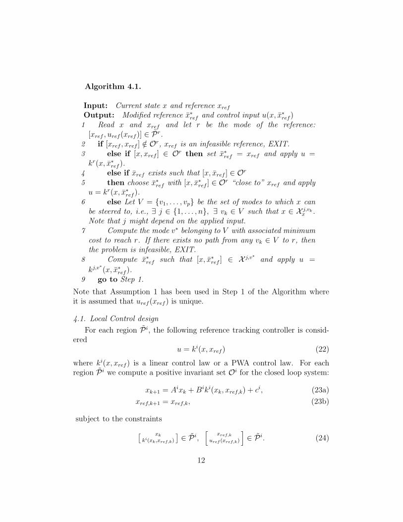
Algorithm 4.1.

Input: Current state x and reference xref

Output: Modified reference x∗ref and control input u(x, x∗ref)1 Read x and xref and let r be the mode of the reference:

[xref , uref(xref)] ∈ Pr.2 if [xref , xref ] /∈ Or, xref is an infeasible reference, EXIT.3 else if [x, xref ] ∈ Or then set x∗ref = xref and apply u =kr(x, x∗ref ).

4 else if xref exists such that [x, xref ] ∈ Or

5 then choose x∗ref with [x, x∗ref ] ∈ Or “close to” xref and applyu = kr(x, x∗ref ).

6 else Let V = {v1, . . . , vp} be the set of modes to which x canbe steered to, i.e., ∃ j ∈ {1, . . . , n}, ∃ vk ∈ V such that x ∈ X j,vk

x .Note that j might depend on the applied input.

7 Compute the mode v∗ belonging to V with associated minimumcost to reach r. If there exists no path from any vk ∈ V to r, thenthe problem is infeasible, EXIT.

8 Compute x∗ref such that [x, x∗ref ] ∈ X j,v∗ and apply u =

kj,v∗(x, x∗ref ).9 go to Step 1.

Note that Assumption 1 has been used in Step 1 of the Algorithm whereit is assumed that uref(xref) is unique.

4.1. Local Control design

For each region P i, the following reference tracking controller is consid-ered

u = ki(x, xref) (22)

where ki(x, xref) is a linear control law or a PWA control law. For eachregion P i we compute a positive invariant set Oi for the closed loop system:

xk+1 = Aixk +Biki(xk, xref,k) + ci, (23a)

xref,k+1 = xref,k, (23b)

subject to the constraints

[ xk

ki(xk ,xref,k)

]

∈ P i,[

xref,k

uref (xref,k)

]

∈ P i. (24)

12

We remark that Oi is a set in the [x, xref ] space. We assume that ki guar-antees the convergence of x(k) to a constant reference xref for system (23).

In addition to standard linear control design techniques, the controllerki(x, xref) can be designed as a receding horizon controller. Consider thefollowing optimal control problem in mode i (denoted as “Problem i”) withhorizon Ni.

J∗,i0 (x(0), xref) , min

UNi

J(UNi, x(0), xref)

subj. to

xk+1 = Aixk +Biuk + ci

[ xkuk

] ∈ P i,[ xref

uref

]

∈ P i

k = 0, . . . , Ni − 1

[xNi, xref ] ∈ X i

f

x0 = x(0).

(25)

Denote by X i0 the feasible set of initial conditions for Problem i (25) and

the associated PWA RHC control law

ki(x, xref) = u∗0(x, xref ) for x ∈ X i0. (26)

If persistent feasibility and convergence are ensured, then X i0 is a positive

invariant set for system (23)-(24) and x(k) → xref and we set Oi = X i0.

We refer the reader to [16] for a discussion on the properties of Problem iguaranteeing that x(k) → xref for k → ∞.

Remark 2. Note that in problem (16)-(18) the terminal set Xf is an invari-ant set for the PWA system (10). In problem (25) X i

f is a “local” invariant

set, i.e., an invariant in mode i. X if is empty if

[

xref

uref (xref )

]

/∈ P i.

Assume[ xref

uref

]

∈ P i. If [ x0xref ] ∈ Oi then the controller ki(x, xref) will

(i) guarantee constraint satisfaction at all time instants, (ii) keep the systemin mode i and (iii) guarantee convergence to

[ xrefuref

]

(step 3 of the OnlineAlgorithm). If [ x0

xref ] /∈ Oi then the local controller ki will not guaranteefeasibility and will not drive x0 towards xref . However, two cases are possible:

1. a xref might exist such that[ x0

xref

]

∈ Oi

2. a u such that [ x0

u ] ∈ P l and a “transition controller” kl,i(x, xref) thatsteers the system from mode l to mode i through a modified xref .

In the both cases feasibility can be guaranteed by computing a new referencexref . The second case requires “transition controllers”. The design of suchcontrollers is described next.

13

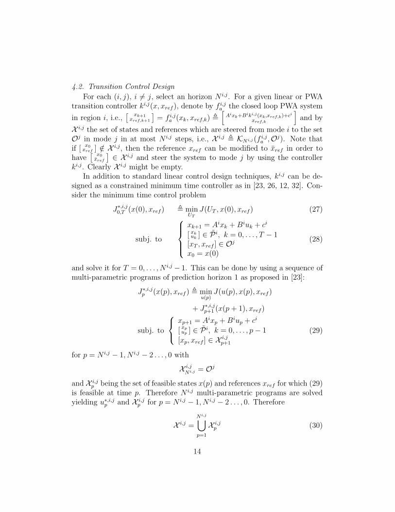
4.2. Transition Control Design

For each (i, j), i 6= j, select an horizon N i,j . For a given linear or PWAtransition controller ki,j(x, xref), denote by f i,j

a the closed loop PWA system

in region i, i.e.,[ xk+1

xref,k+1

]

= f i,ja (xk, xref,k) ,

[

Aixk+Biki,j(xk,xref,k)+ci

xref,k

]

and by

X i,j the set of states and references which are steered from mode i to the setOj in mode j in at most N i,j steps, i.e., X i,j , KN i,j (f i,j

a ,Oj). Note thatif [ x0

xref ] /∈ X i,j, then the reference xref can be modified to xref in order tohave

[ x0

xref

]

∈ X i,j and steer the system to mode j by using the controllerki,j. Clearly X i,j might be empty.

In addition to standard linear control design techniques, ki,j can be de-signed as a constrained minimum time controller as in [23, 26, 12, 32]. Con-sider the minimum time control problem

J∗,i,j0,T (x(0), xref) , min

UT

J(UT , x(0), xref) (27)

subj. to

xk+1 = Aixk +Biuk + ci

[ xkuk

] ∈ P i, k = 0, . . . , T − 1[xT , xref ] ∈ Oj

x0 = x(0)

(28)

and solve it for T = 0, . . . , N i,j − 1. This can be done by using a sequence ofmulti-parametric programs of prediction horizon 1 as proposed in [23]:

J∗,i,jp (x(p), xref ) , min

u(p)J(u(p), x(p), xref)

+ J∗,i,jp+1 (x(p + 1), xref)

subj. to

xp+1 = Aixp +Biup + ci

[xpup ] ∈ P i, k = 0, . . . , p− 1

[xp, xref ] ∈ X i,jp+1

(29)

for p = N i,j − 1, N i,j − 2 . . . , 0 with

X i,j

N i,j = Oj

and X i,jp being the set of feasible states x(p) and references xref for which (29)

is feasible at time p. Therefore N i,j multi-parametric programs are solvedyielding u∗,i,jp and X i,j

p for p = N i,j − 1, N i,j − 2 . . . , 0. Therefore

X i,j =N i,j⋃

p=1

X i,jp (30)

14

Note that since N i,j multi-parametric programs are solved, several controllerregions in X i,j

p may overlap. In order to guarantee minimum-time conver-gence and feasibility, the feedback law u∗,i,jc associated with the region com-puted at the smallest horizon c is selected for any given state x. More detailscan be found in [23].

Recall that X i,jx is the projection of X i,j on the x space. Similarly, X i,j

x,p

is the projection of X i,jp on the x space. If x belongs to X i,j

x,p then there exista reference which will bring the PWA system from mode i to the invariantset Oj in mode j in p steps.

4.3. The Weighted Graph

For each mode we have designed a local controller ki and computed acorresponding invariant Oi. For each pair of modes we have designed atransition controller ki,j and computed a set X i,j of states and references inmode i which reach Oj in mode j in at most N i,j steps.

Clearly, if the current state is in mode i1 and the reference in mode in, thesystem could still be controlled to the reference even if X i1,in is empty. There-fore, the last step is to compute the optimal transition sequence i1, i2, . . . , inbetween any two modes i1 and in. We propose to use the properties of thesets Oi and X i,j in order to avoid the inherent exponential complexity of theproblem at the price of smaller regions of attraction.

In particular we can move from i1 to i2 through the set X i1,i2 by usingki1,i2 . Then, when the system is in mode i2, we can move through the setOi2 by using ki2 and reach X i2,i3 and so on. In this way input and stateconstraints are always satisfied. The feasibility property of this approach isdescribed in following proposition.

Proposition 1. Let Assumption 1 hold, x(k) be the current system stateand xref the current reference. Assume that [xref , uref(xref)] is in mode j.Assume that x(k) ∈ ProjxO

i. Define the set X i,j as

X i,j , ProjxOi⋂

Projx{

[x, xref ] ∈ X i,j| x = xref

}

(31)

If X i,j is not empty, then there exists a time varying reference and a feasiblestate feedback control law such that the system (14) with initial state x(k) inmode i can be steered to the set Oj in mode j.

Proof.

15

We consider two cases: x(k) ∈ Projx(Xi,j) and x(k) /∈ Projx(X

i,j).If x(k) ∈ Projx(X

i,j) then compute xref such that [x(k), xref ] ∈ X i,j

and apply ki,j(x(k), xref ). By construction of X i,j, there exists a sequence ofreferences such that the state will reach Oj in at most N i,j steps.

Assume x(k) /∈ Projx(Xi,j). By assumption x(k) ∈ Projx(O

i), andX i,j is not empty. Therefore the system can say in Oi (and thus satisfyconstraints) and by changing the reference it can reach a new state xref withthe property xref ∈ Projx(X

i,j).

Pick[

xref

xref

]

∈ X i,j with xref ∈ X i,j and solve the following problem

xref , arg minxref(‖xref − xref‖) (32a)

subj. to[

x(k)xref

]

∈ Oi (32b)

Problem (32) is feasible since by assumption x(k) ∈ Projx(Oi). Note

however that [x(k), xref ] might not belong to Oi. Apply ki(x, xref ). Since(x(k), xref) ∈ Oi then limk→+∞ x(k) = xref and since Oi is a connected set,

limk→+∞ xref → xref with[

xref

xref

]

∈ X i,j. 2

Proposition 1 shows that we can transition from mode i to mode jfrom X i,j or from Oi if X i,j is not empty. Therefore one can steer thestate from mode i1 to mode in by applying the sequence of controllerski1,i2 , ki2 ,ki2,i3, ki3 ,. . .,kin.

The concept of weighted graph will be used to compute the “best” tran-sition sequence from Oi to Oj for any two modes i, j. A weighted graph Gis defined as

G = (V,A) (33)

where V is the set of nodes (or vertices) V = {1, . . . , N} and A ⊆ V ×V theset of edges (i, j) with i ∈ V, j ∈ V. Let Ai,j ∈ R be the i, j element of theweighted adjacency matrix A of the graph G. If there is no edge connectingthe vertex i with the vertex j, i.e., (i, j) /∈ A, we set Ai,j = 0.

The elements of A are computed as follows:

ai,j = α1

vol(X i,j)+ βN i,j (34)

where vol(P) is the volume of the polyhedron P. The positive real num-bers α and β are tuning parameters. Given the weighted graph G, u =

16

SPath(G, i1, in) is the vector which describes the shortest path

u = {i1, i2, . . . , in} between node i1 and node in and SPathCost(G, i1, in)is the corresponding optimal cost.

Clearly, several other alternatives to the weight choice in (34) can beproposed depending on the specific application. The weights in (34) captureonly two important elements: the time to reach the target region and thesize of the feasible set which generates a transition. The latter can be seen asa practical measure on how robust to system uncertainties and measurementnoise the transition is.

4.4. On-line Reference Governor Algorithm

Once all the elements have been computed off-line, the following algo-rithm is implemented on-line.

17

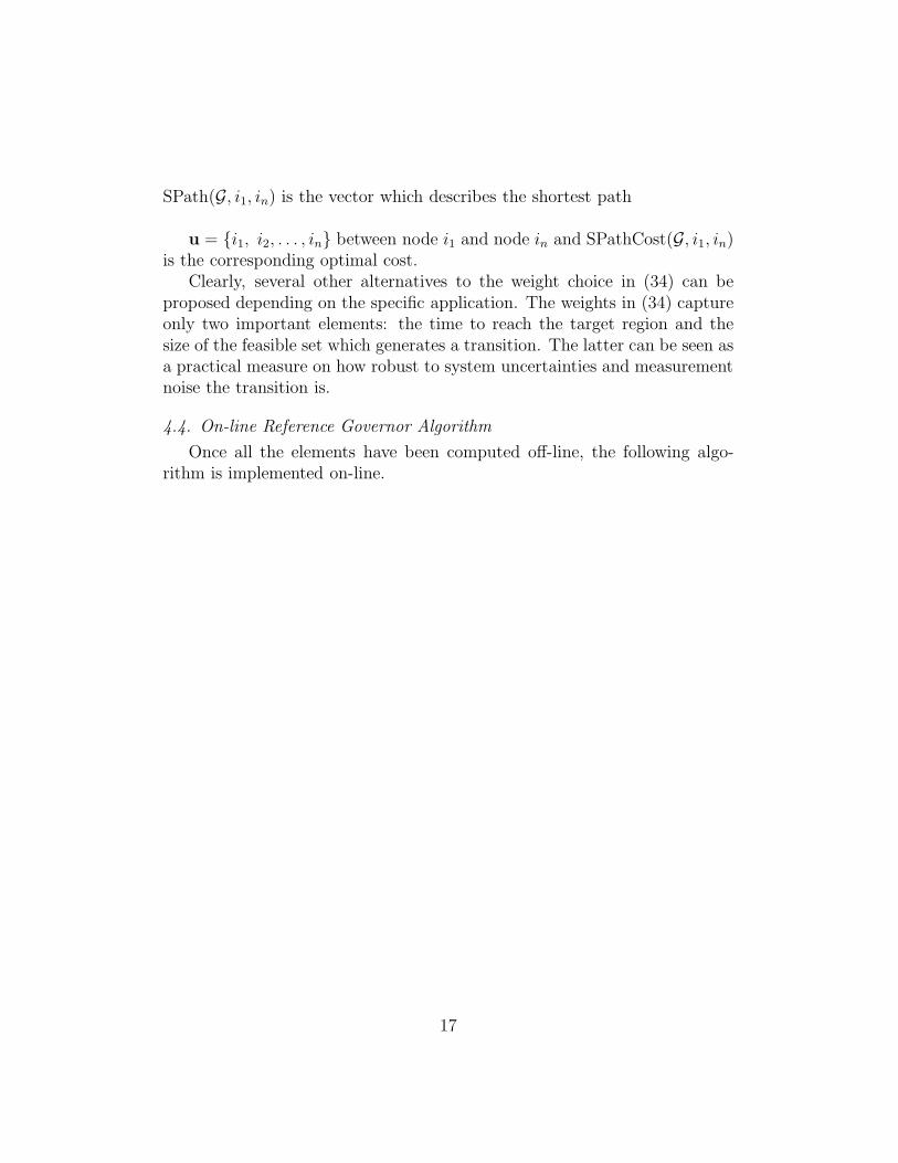
Algorithm 4.2.

Input: Current state x(t) and reference xref = xref(t)Output: Modified reference x∗ref(t) and controller selection

1 let r be such that [xref , xref ] ∈ Or

2 if x(t) ∈ Projx(Or) then select local controller kr and compute

the modified reference as follows

x∗ref = arg minxref‖xref − xref‖ (35a)

subj. to[

x(t)xref

]

∈ Or (35b)

3 else4 let v = {v1, . . . , vn} the set of modes such that x(t) ∈Projx(X

l,vi) and let u = {u1, . . . , um} the set of modes such thatx(t) ∈ Projx(O

ui). (note that x(t) can be in multiple modes becausethe system partition depends on the input as well).

5 Compute v∗ ∈ v ∪ u with the associated shortest path{v∗, i1, . . . , in, r} and cost s∗ = SPathCost(G, v∗, r).

6 if s∗ = ∞ then “Infeasible Reference”, EXIT7 if v∗ ∈ v then select transition controller kl,v∗ and compute

the modified reference as follows

x∗ref = arg minxref‖xref − xref‖ (36)

subj. to[

x(t)xref

]

∈ X l,v∗ (37)

8 else select local controller kv∗ and compute the modified refer-ence as follows

x∗ref , arg minxref ,xref(‖xref − xref‖) (38)

subj. to[

x(t)xref

]

∈ Ov∗ (39)[

xref

xref

]

∈ X v∗,i1 (40)

9 go to Step 1

Remark 3. Note that the sets X i,j might be described as the union of poly-

18

hedra X i,jk , for k = 1, . . . , N i,j where X i,j

k represents the k − steps reachableset. In this case, Step 7 in Algorithm 4.2 can be modified as follows:

x∗ref = arg minxref ,k ‖xref − xref‖ (41a)

subj. to[

x(t)xref

]

∈ X l,v∗

k (41b)

The same modification can be applied to Step 8 in Algorithm 4.2.

Remark 4. Note that the QP problem defined in Step 2 in Algorithm 4.2can be solved explicitly as has been shown in [36, 34].

Remark 5. Consider step 5 of Algorithm 4.2. If there exists multiple v∗

yielding s∗ = SPathCost(G, v∗, r), then a v∗ will be used. In this case cyclingcould occur but it can easily be avoided by storing modes which have beenalready explored.

5. Numerical Example

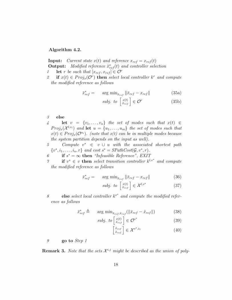
A simple vehicle dynamics example is presented next. We consider abicycle model of a vehicle sketched in Figure 1 and refer the reader to [17]for details on modeling and simplifying assumptions.

The lateral and yaw dynamics are described by the following nonlineardifferential equations:

my = −mxψ + 2[

Fyf+ Fyr

]

(42a)

Iψ = 2[

aFyf− bFyr

]

(42b)

where x is the longitudinal speed, y the lateral speed, ψ the yaw rate, Fyf

and Fyrare front and rear tire lateral forces, respectively.

The front and rear tire slip angles are approximated as:

αf = δf −y + aψ

x(43a)

αr =bψ − y

x(43b)

where δf is the vehicle steering angle and it is the system input.

19

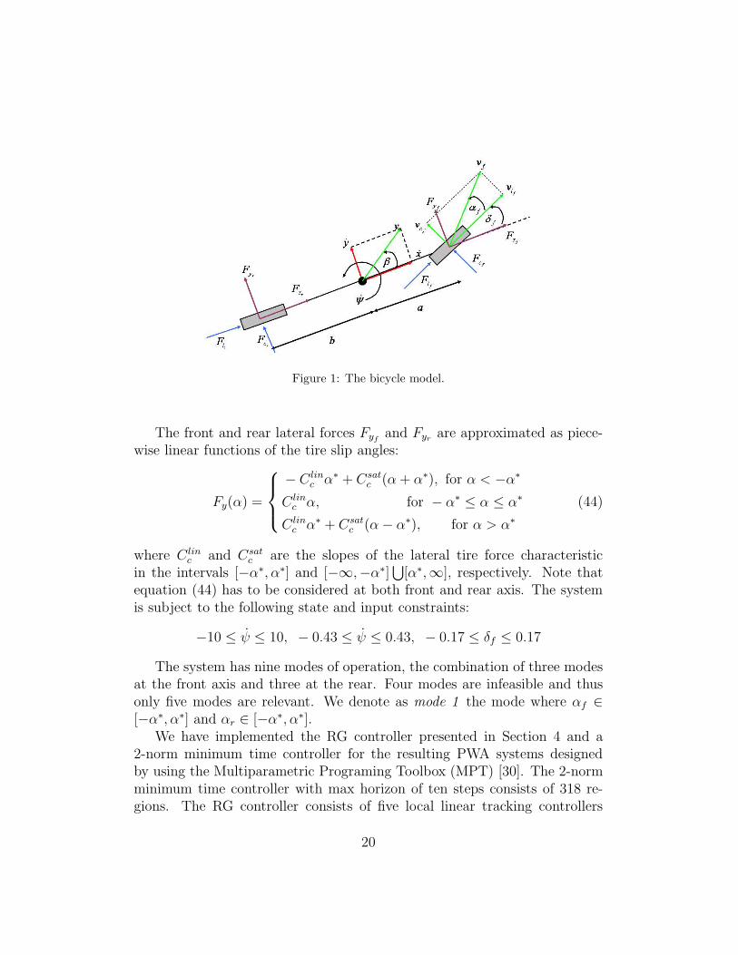
Figure 1: The bicycle model.

The front and rear lateral forces Fyfand Fyr

are approximated as piece-wise linear functions of the tire slip angles:

Fy(α) =

− C linc α∗ + Csat

c (α+ α∗), for α < −α∗

C linc α, for − α∗ ≤ α ≤ α∗

C linc α∗ + Csat

c (α− α∗), for α > α∗

(44)

where C linc and Csat

c are the slopes of the lateral tire force characteristicin the intervals [−α∗, α∗] and [−∞,−α∗]

⋃

[α∗,∞], respectively. Note thatequation (44) has to be considered at both front and rear axis. The systemis subject to the following state and input constraints:

−10 ≤ ψ ≤ 10, − 0.43 ≤ ψ ≤ 0.43, − 0.17 ≤ δf ≤ 0.17

The system has nine modes of operation, the combination of three modesat the front axis and three at the rear. Four modes are infeasible and thusonly five modes are relevant. We denote as mode 1 the mode where αf ∈[−α∗, α∗] and αr ∈ [−α∗, α∗].

We have implemented the RG controller presented in Section 4 and a2-norm minimum time controller for the resulting PWA systems designedby using the Multiparametric Programing Toolbox (MPT) [30]. The 2-normminimum time controller with max horizon of ten steps consists of 318 re-gions. The RG controller consists of five local linear tracking controllers

20

ki(x, xref) designed by using LQR techniques. We used the local controllersas transition controllers, i.e., ki,j(x, xref) = ki(x, xref ) for all j = 1, . . . , 5.With this choice, the only non-empty transition sets reach mode 1. There-fore the RG controller requires five local invariant sets O1

∞, . . . ,O5

∞, and ten

transition sets X 2,11 ,X 2,1

2 , X 2,13 , X 3,1

1 , X 3,12 , X 3,1

3 , X 4,11 , X 4,1

2 , X 5,11 , X 5,1

2 . Weremark that transition sets with longer horizons are empty.

Figure 2 depicts the feasible sets for both controllers. As expected, theprice of complexity reduction is paid with a smaller feasibility region. Weremark that in both cases the feasible area is also the region of attraction forthe closed loop system.

y

ψ

-3.5 -3 -2.5 -2 -1.5 -1 -0.5 0 0.5 1 1.5

-0.4

-0.3

-0.2

-0.1

0

0.1

0.2

0.3

0.4

(a) Feasible set of the RG controller de-scribed in Section 4

y

ψ

-3 -2 -1 0 1

-0.4

-0.2

0

0.2

0.4

(b) Feasible set of a 2-norm minimumtime controller (318 regions)

Figure 2: Comparison of feasible domains for the RG controller and an explicitminimum-time controller

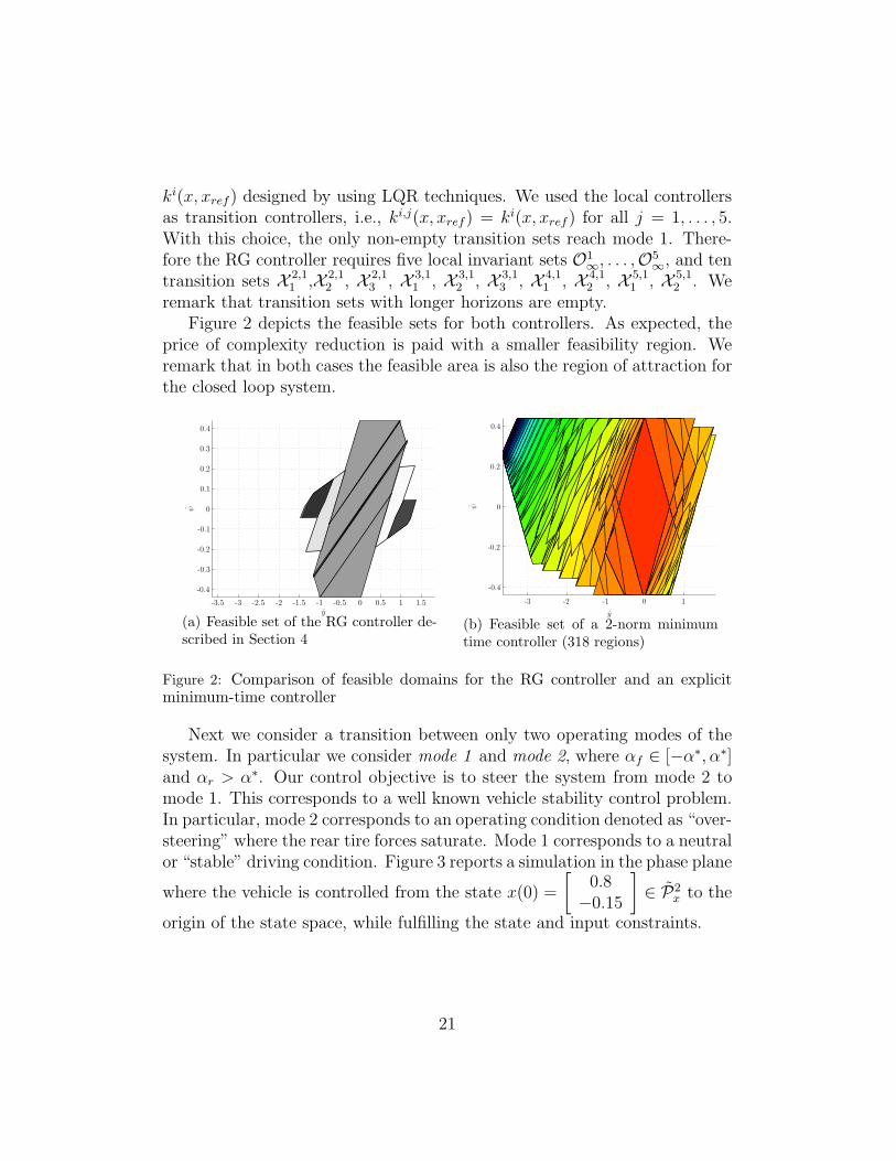
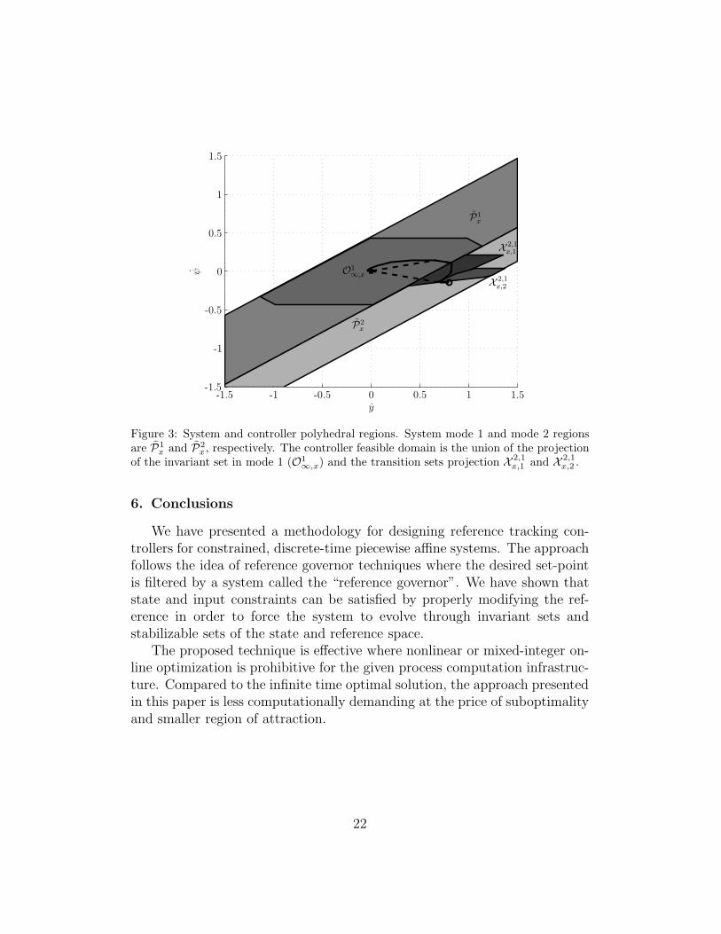
Next we consider a transition between only two operating modes of thesystem. In particular we consider mode 1 and mode 2, where αf ∈ [−α∗, α∗]and αr > α∗. Our control objective is to steer the system from mode 2 tomode 1. This corresponds to a well known vehicle stability control problem.In particular, mode 2 corresponds to an operating condition denoted as “over-steering” where the rear tire forces saturate. Mode 1 corresponds to a neutralor “stable” driving condition. Figure 3 reports a simulation in the phase plane

where the vehicle is controlled from the state x(0) =

[

0.8−0.15

]

∈ P2x to the

origin of the state space, while fulfilling the state and input constraints.

21

y

ψ

P1x

P2x

O1∞,x

X 2,1x,1

X 2,1x,2

-1.5 -1 -0.5 0 0.5 1 1.5-1.5

-1

-0.5

0

0.5

1

1.5

Figure 3: System and controller polyhedral regions. System mode 1 and mode 2 regionsare P1

xand P2

x, respectively. The controller feasible domain is the union of the projection

of the invariant set in mode 1 (O1

∞,x) and the transition sets projection X 2,1

x,1and X 2,1

x,2.

6. Conclusions

We have presented a methodology for designing reference tracking con-trollers for constrained, discrete-time piecewise affine systems. The approachfollows the idea of reference governor techniques where the desired set-pointis filtered by a system called the “reference governor”. We have shown thatstate and input constraints can be satisfied by properly modifying the ref-erence in order to force the system to evolve through invariant sets andstabilizable sets of the state and reference space.

The proposed technique is effective where nonlinear or mixed-integer on-line optimization is prohibitive for the given process computation infrastruc-ture. Compared to the infinite time optimal solution, the approach presentedin this paper is less computationally demanding at the price of suboptimalityand smaller region of attraction.

22

7. Acknowledgements

The authors are grateful to the anonymous reviewers for their helpfulcomments on the original version of this manuscript.

References

[1] M. Baotic, F. Borrelli, A. Bemporad, and M. Morari. Efficient on-linecomputation of constrained optimal control. SIAM Journal on Controland Optimization, 47:2470–2489, 2008.

[2] A. Bemporad. Reference governor for constrained nonlinear systems.Automatic Control, IEEE Transactions on, 43(3):415–419, Mar 1998.

[3] A. Bemporad, A. Casavola, and E. Mosca. Nonlinear control of con-strained linear systems via predictive reference management. AutomaticControl, IEEE Transactions on, 42(3):340–349, Mar 1997.

[4] A. Bemporad and M. Morari. Control of systems integrating logic, dy-namics, and constraints. Automatica, 35(3):407–427, March 1999.

[5] A. Bemporad, M. Morari, V. Dua, and E.N. Pistikopoulos. The explicitlinear quadratic regulator for constrained systems. Automatica, 38(1):3–20, 2002.

[6] A. Bemporad and E. Mosca. Constraint fulfilment in feedback controlvia predictive reference management. Control Applications, 1994., Pro-ceedings of the Third IEEE Conference on, pages 1909–1914 vol.3, Aug1994.

[7] A. Bemporad and E. Mosca. Constraint fulfilment in feedback controlvia predictive reference management. Control Applications, 1994., Pro-ceedings of the Third IEEE Conference on, pages 1909–1914 vol.3, Aug1994.

[8] A. Bemporad and E. Mosca. Nonlinear predictive reference governor forconstrained control systems. Decision and Control, 1995., Proceedingsof the 34th IEEE Conference on, 2:1205–1210 vol.2, Dec 1995.

[9] D. P. Bertsekas. Control of Uncertain Systems with a set–membershipdescription of the uncertainty. PhD thesis, MIT, 1971.

23

[10] D. P. Bertsekas and I. B. Rhodes. On the minimax reachability of targetsets and target tubes. Automatica, 7:233–247, 1971.

[11] L.T. Biegler and V.M. Zavala. Large-scale nonlinear programming usingipopt: An integrating framework for enterprise-wide dynamic optimiza-tion. Computers & Chemical Engineering, 33(3):575 – 582, 2009. Se-lected Papers from the 17th European Symposium on Computer AidedProcess Engineering held in Bucharest, Romania, May 2007.

[12] F. Blanchini. Minimum-time control for uncertain discrete-time linearsystems. In Proc. 31rd IEEE Conf. on Decision and Control, pages2629–2634, Tucson, Arizona, USA, December 1992.

[13] F. Blanchini. Set invariance in control — a survey. Automatica,35(11):1747–1768, November 1999.

[14] F. Borrelli. Constrained Optimal Control of Linear & Hybrid Systems,volume 290. Springer Verlag, 2003.

[15] F. Borrelli, M. Baotic, A. Bemporad, and M. Morari. Dynamic program-ming for constrained optimal control of discrete-time hybrid systems.Automatica, 41:1709–1721, January 2005.

[16] F. Borrelli and M. Morari. Offset free model predictive control. InDecision and Control, 2007 46th IEEE Conference on, pages 1245–1250,Dec. 2007.

[17] P. Falcone, F. Borrelli, J. Asgari, H. E. Tseng, and D. Hrovat. Predictiveactive steering control for autonomous vehicle systems. IEEE Trans. onControl System Technology, 15(3), 2007.

[18] H.J. Ferreau and M. Diehl H.G. Bock. An online active set strategyto overcome the limitations of explicit mpc. International Journal ofRobust and Nonlinear Control, 18:816–830, 2008.

[19] A. V. Fiacco. Introduction to sensitivity and stability analysis in non-linear programming. Academic Press, London, U.K., 1983.

[20] E. G. Gilbert and K. T. Tan. Linear systems with state and controlconstraints: The theory and application of maximal output admissiblesets. IEEE Trans. Automatic Control, 36(9):1008–1020, September 1991.

24

[21] E.G. Gilbert and I. Kolmanovsky. A generalized reference governor fornonlinear systems. Decision and Control, 2001. Proceedings of the 40thIEEE Conference on, 5:4222–4227 vol.5, 2001.

[22] E.G. Gilbert, I. Kolmanovsky, and Kok Tin Tan. Nonlinear controlof discrete-time linear systems with state and control constraints: areference governor with global convergence properties. Decision andControl, 1994., Proceedings of the 33rd IEEE Conference on, 1:144–149vol.1, Dec 1994.

[23] P. Grieder. Efficient Computation of Feedback Controllers for Con-strained Systems. PhD thesis, ETH-Zurich, Automatic Control Lab-oratory, 2004.

[24] P. Grieder and M. Morari. Complexity reduction of receding horizoncontrol. In IEEE Conference on Decision and Control, pages 3179–3184,Maui, Hawaii, December 2003.

[25] C. Jones, P. Grieder, and S. Rakovic. A logarithmic-time solution tothe point location problem for closed-form linear MPC. In IFAC WorldCongress, Prague, Czech Republic, 2009.

[26] S.S. Keerthi and E.G. Gilbert. Computation of minimum-time feedbackcontrol laws for discrete-time systems with state-control constraints.IEEE Trans. Automatic Control, AC-32:432–435, May 1987.

[27] E. C. Kerrigan. Robust Constraints Satisfaction: Invariant Sets andPredictive Control. PhD thesis, Department of Engineering, Universityof Cambridge, Cambridge, England, 2000.

[28] I. Kolmanovsky and E. G. Gilbert. Theory and computation of dis-turbance invariant sets for discrete-time linear systems. MathematicalProblems in Egineering, 4:317–367, 1998.

[29] I. Kolmanovsky and Jing Sun. Approaches to computationally efficientimplementation of gain governors for nonlinear systems with pointwise-in-time constraints. Decision and Control, 2005 and 2005 EuropeanControl Conference. CDC-ECC ’05. 44th IEEE Conference on, pages7564–7569, Dec. 2005.

25

[30] M. Kvasnica, P. Grieder, and M. Baotic. Multi-Parametric Toolbox(MPT). http://control.ee.ethz.ch/mpt/, 2004.

[31] J. Lygeros, C. Tomlin, and S. Sastry. Controllers for reachability speci-fications for hybrid systems. Automatica, 35(3):349–370, 1999.

[32] D. Q. Mayne and W. R. Schroeder. Robust time–optimal control ofconstrained linear systems. Automatica, 33(12):2103–2118, 1997.

[33] D.Q. Mayne, J.B. Rawlings, C.V. Rao, and P.O.M. Scokaert. Con-strained model predictive control: Stability and optimality. Automatica,36(6):789–814, June 2000.

[34] S. Olaru and D. Dumur. Compact explicit MPC with guarantee of fea-sibility for tracking. In Proc. 44th IEEE Conf. on Decision and Control,pages 969–974, 2005.

[35] G. Pannocchia and J. B. Rawlings. Disturbance models for offset-freemodel predictive control. AIChE Journal, 49(2):426–437, 2003.

[36] J. Pekar and V. Havlena. Model predictive control with invariant sets:Set-point tracking. In Proc. of 15th International Conference of ProcessControl 05, 2005.

[37] Sasa V. Rakovic. Robust Control of Constrained Discrete Time Sys-tems: Characterization and Implementation. PhD thesis, Imperial Col-lege London, London, United Kingdom, July 2005.

[38] Lino O. Santos, Paulo A. F. N. A. Afonso, Jos A. A. M. Castro, NunoM. C. Oliveira, and Lorenz T. Biegler. On-line implementation of non-linear mpc: an experimental case study. Control Engineering Practice,9(8):847 – 857, 2001.

[39] E.D. Sontag. Nonlinear regulation: The piecewise linear approach. IEEETrans. Automatic Control, 26(2):346–358, April 1981.

[40] A. Vahidi, I. Kolmanovsky, and A. Stefanopoulou. Constraint handlingin a fuel cell system: A fast reference governor approach. Control Sys-tems Technology, IEEE Transactions on, 15(1):86–98, Jan. 2007.

26