- 1 -

Refined resultant thermomechanics of shells

W. PIETRASZKIEWICZ

Institute of Fluid-Flow Machinery, PASci, ul. Fiszera 14, 80-952 Gdańsk, Poland

Email: pietrasz@imp.gda.pl Phone: (+48) 58 69 95 263 Fax: (+48) 58 341 61 44

Abstract The resultant two-dimensional (2D) balance laws of mass, linear and angular momentum, and energy as well as the entropy inequality for shells are derived by direct through-the-thickness integration of corresponding 3D laws of continuum thermomechanics. It is indicated that the resultant shell stress power cannot be expressed exactly through the 2D shell stress and strain measures alone. Hence, an additional stress power called an interstitial working is added to the resultant 2D balance of energy. The new, refined, resultant balance of energy and entropy inequality derived here are regarded to be exact implications of corresponding global 3D laws of rational thermodynamics. The kinematic structure of our shell theory is that of the Cosserat surface, while our refined resultant laws of thermomechanics contain three additional surface fields somewhat similar to those present in 3D extended thermodynamics. We briefly analyse the restrictions imposed by our refined resultant entropy inequality on the forms of 2D constitutive equations of viscous shells with heat conduction and of thermoelastic shells. It is shown, in particular, that in such shells the refined resultant entropy inequality allows one to account for some longer-range spatial interactions. We also present several novel forms of 2D kinetic constitutive equations compatible with the resultant shell equations.

Keywords Shell thermomechanics, Resultant formulation, Cosserat surface, Extended thermomechanics, Constitutive equations, Viscous shells, Thermoelastic shells, Kinetic constitutive equations

1. Introduction Non-linear, thermomechanic, two-dimensional (2D) models of shells are usually developed using

two main approaches: 1) the so-called direct formulation, and 2) the derived or deductive formulation

from three-dimensional (3D) continuum mechanics. But the basic 2D relations of shell

thermomechanics and physical interpretation of their ingredients vary substantially throughout the

literature. The direct approach, performed along the lines of mechanical model of the surface proposed

by Cosserat (1909), was used for example by Naghdi (1972); Zhilin (1976); Murdoch (1976); Rubin

(1999); Eremeyev and Zubov (2008). In the deductive approach one usually expands all 3D fields into

series of thickness coordinate and then assumes some kinematic, dynamic and/or thermal constraints

- 2 -

to make the 2D complex shell relations more accessible for applications, see for example Green and

Naghdi (1970, 1979); Krätzig (1971); Naghdi (1972); Kleiber and Woźniak (1991). In both

approaches the errors of such 2D thermomechanic shell relations are practically indefinable.

The resultant shell thermomechanics proposed concisely by Simmonds (1984) deserves special

attention, because :

1. The resultant balance laws of mass, linear and angular momentum, and energy as well as the

entropy inequality were formulated on the shell base surface by exact through-the-thickness

integration of appropriate 3D laws of continuum thermomechanics.

2. The shell kinematics was constructed uniquely through the virtual work identity. This resulted

in the translation vector and the rotation tensor fields as the only independent kinematic

variables describing the gross motion of the shell cross section.

3. The only approximations were made in the resultant balance of energy when expressed

through the 2D fields alone. The errors were then transferred onto the resultant entropy

inequality and the 2D constitutive equations, which are experimental laws anyway.

The mechanical part of such resultant shell theory, originally proposed by Reissner (1974), gained

considerable attention in the literature, and many results obtained in the field are now partly

summarised for example in the books by Libai and Simmonds (1998); Chróścielewski et al. (2004);

Eremeyev and Zubov (2008). But the resultant approach to shell thermomechanics of Simmonds

(1984) seems still to be insufficiently publicised and used in thermomechanic shell analyses. Among a

few papers in this field let us mention the report by Makowski and Pietraszkiewicz (2002) on possible

generalizations of the resultant approach and papers by Eremeyev and Pietraszkiewicz (2009, 2010) on

thermomechanics of phase transitions in shells.

In this paper the local, exact, resultant balance laws of mass, linear and angular momentum, and

energy as well as the entropy inequality for shells are derived by direct through-the-thickness

integration of corresponding 3D laws of continuum thermodynamics. Our resultant laws are

formulated in the referential description on the shell base surface which is taken to be the material

surface during shell motion, not a non-material mass-weighted surface as in Simmonds (1984).

In section 3 it is shown that approximations of the resultant balance of energy follow from

impossibility to represent exactly the resultant mechanical power, stress power, and kinetic energy

using the surface fields alone. In particular, Pietraszkiewicz et al. (2005) proved explicitly that, when

reduced to the base surface, the shell stress power S consists of two parts: a) the effective stress

power eS performed by the resultant 2D shell stress measures ,N M on appropriate time rates of the

work-conjugate 2D shell strain measures ,E K , and 2) an additional stress power not expressible

through the surface fields. In order to restore the full amount of stress power of the shell, an additional

mechanical power W such that e= +S S W , called an interstitial working after Dunn and Serrin

(1985), is introduced on the 2D level. With the corresponding interstitial flux vector field w our new,

- 3 -

refined, resultant balance of energy (48) becomes an exact implication of the global 3D balance of

energy. It refines the effective energy balance, which is inaccurate when expressed through the surface

fields alone and then analogous to that formulated by Simmonds (1984).

The exact, resultant 2D entropy inequality (57) is derived in section 4 by integrating through the

thickness the 3D Clausius-Duhem inequality proposed by Truesdell and Toupin (1960). Then our

refined 2D balance of energy (48) is used to transform the inequality (57) into another form more

convenient for discussing the 2D constitutive equations. The transformed resultant entropy inequality

(60) is also new in the literature and refines the analogous one proposed by Simmonds (1984). It can

be regarded as an exact implication of the global 3D Clausius-Duhem inequality as well.

Although on 3D level we begin with the classical Cauchy continuum and the Clausius-Duhem

inequality of rational thermomechanics, our refined resultant relations of shell thermomechanics do

not remind the classical ones. The kinematic structure of the resultant shell theory is that of the

Cosserat (1909) surface, which was noted already by Reissner (1974). Our two novel, refined resultant

laws of shell thermomechanics contain three additional surface fields. The structure of these 2D laws

of shell thermomechanics reminds somewhat that of corresponding 3D laws of extended

thermodynamics, see for example Müller and Ruggeri (1998).

In section 5 the procedure of Coleman and Noll (1963) is used to analyse restrictions imposed by

our refined entropy inequality (60) on the 2D forms of constitutive equations. As examples, we briefly

discuss viscous shells with heat conduction and thermoelastic shells defined here by the extended

constitutive equations, in which also the possibility of longer-range spatial interactions is accounted

for. It is shown, in particular, that our resultant entropy inequality does allow the constitutive

equations to depend also on the first surface gradients of the shell strain measures and on the second

surface gradient of the referential surface temperature. Finally, several novel forms of the 2D kinetic

constitutive equations obtained with the help of heuristic arguments are provided.

2. Basic principles of resultant thermomechanics for shells

Within 3D continuum thermodynamics we assume that all material bodies possess mass, sustain

forces and torques, convert energy, and basic laws of thermodynamics are valid for any part P of the

body B .

To describe the mechanical behaviour of P at any time t T∈ we assume the following primitive

quantities to be meaningful: the mass ( , )tM P , the mass production ( , )tC P , the linear momentum

vector ( , )tL P , the total force vector ( , )tF P , the angular momentum vector o ( , )tA P , and the total

torque vector o ( , )tT P . The latter two quantities are defined in an inertial frame (o, )ie relative to a

point o of the three-dimensional (3D) physical space E with V as its translation 3D vector space, and

where i V∈e , 1,2,3i = , are orthonormal vectors. The primitive quantities are assumed to satisfy three

- 4 -

balance laws of continuum mechanics: balances of mass, of linear momentum and of angular

momentum, see for example Truesdell and Toupin (1960); Truesdell and Noll (1965). When written in

the most general, global integral-impulse form these laws are:

2 2 22 2 21 1 11 1 1

o o| , | , | .t t tt t t

t t tt t tdt dt dt= = =∫ ∫ ∫M C L F A T (1)

Two latter laws in (1) are given in the inertial frame (o, )ie , and 1 2[ , ]t t T∈ .

When the theory is designed to account for thermal effects, we assume additional primitive

quantities to be meaningful: the total energy ( , )tU P , the heating ( , )tQ P , the entropy ( , )tH P , and the

entropy flux ( , )tJ P . It is generally accepted that these quantities have to satisfy no more than two

laws of continuum thermodynamics. However, while the form of energy balance is universally

accepted, there is no general agreement which specific form should take The 2nd Law. Let us refer to

reviews by Muschik et al. (2001); Muschik (2008) and to recent books by Müller (2007); Badur

(2009), where many references to historic papers and books on various formulations of continuum

thermodynamics are given.

Within the rational thermodynamics developed by Truesdell and Toupin (1960); Truesdell and

Noll (1965); Truesdell (1975, 1984), which we shall use here, the two laws of thermodynamics are the

balance of energy (also called The 1st Law) and the entropy inequality (also called The 2nd Law):

2 22 21 11 1

| ( ) , | ,t tt t

t tt tdt dt= + ≥∫ ∫U P Q H J (2)

where ( , )tP P means the mechanical power, and ( , )tJ P is taken in the Clausius-Duhem form, see

Section 4 below.

In continuum mechanics each placement ( , )tχ P of ∈P B at time t becomes a part P( )t of the

region B( ) ( , )t t= χ B of E . By y P(t)∈ we denote the actual place of material particle and by

y o= −y its position vector in the inertial frame (o, )ie . Then P B⊂ is the region of E occupied by

P in the reference placement κ( )P associated here with 0t = , while x B∈ is the reference place of

material particle and x o= −x its position vector in the same inertial frame (o, )ie .

In the shell-like body the boundary surface B∂ of the reference region B consists of three parts:

the upper M + and the lower M − shell faces, and the lateral boundary surface B*∂ such that

B B*M M+ −∂ = ∪ ∪∂ , M M+ −∩ =∅ . Relative to the origin o∈E of the inertial frame (o, )ie the

position vectors x and y are usually described by

( , ) ( ) ( ) , ( , , ) ( , ) ( , , ) .x x x x t x t x tξ ξ ξ ξ= + = +x y zx n y (3)

Here ( ) ( ,0)x x= xx is the position vector of corresponding point of some reference base surface

M ⊂ E , ( )xn is the unit normal vector orienting M , [ ( ), ( )]h x h xξ − +∈ − is distance along n from

- 5 -

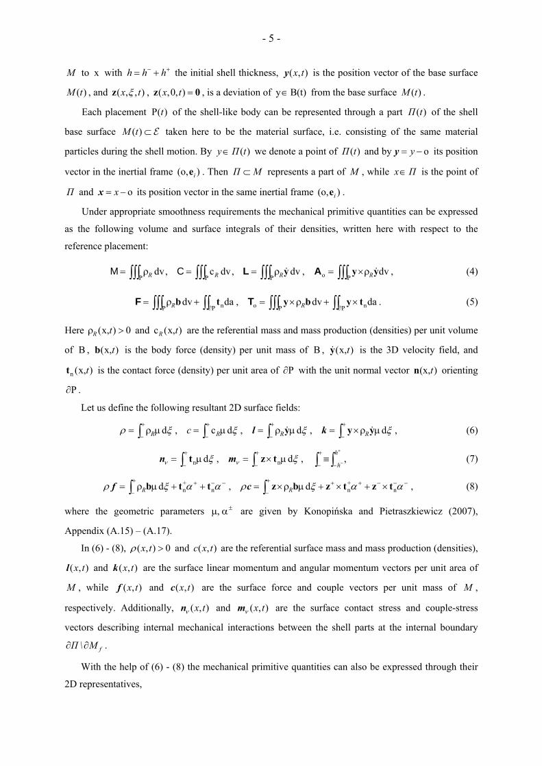
M to x with h h h− += + the initial shell thickness, ( , )x ty is the position vector of the base surface

( )M t , and ( , , )x tξz , ( ,0, )x t =z 0 , is a deviation of y B(t)∈ from the base surface ( )M t .

Each placement P( )t of the shell-like body can be represented through a part ( )Π t of the shell

base surface ( )M t ⊂ E taken here to be the material surface, i.e. consisting of the same material

particles during the shell motion. By ( )y Π t∈ we denote a point of ( )Π t and by oy= −y its position

vector in the inertial frame (o, )ie . Then Π M⊂ represents a part of M , while x Π∈ is the point of

Π and ox= −x its position vector in the same inertial frame (o, )ie .

Under appropriate smoothness requirements the mechanical primitive quantities can be expressed

as the following volume and surface integrals of their densities, written here with respect to the

reference placement:

oP P P Pdv, c dv, dv , dv ,R R R R= ρ = = ρ = ×ρ∫∫∫ ∫∫∫ ∫∫∫ ∫∫∫y y yM C L A (4)

n o nP P P Pdv da , dv da .R R∂ ∂

= ρ + = ×ρ + ×∫∫∫ ∫∫ ∫∫∫ ∫∫b t y b y tF T (5)

Here (x, ) 0R tρ > and c (x, )R t are the referential mass and mass production (densities) per unit volume

of B , (x, )tb is the body force (density) per unit mass of B , (x, )ty is the 3D velocity field, and

n (x, )tt is the contact force (density) per unit area of P∂ with the unit normal vector (x, )tn orienting

P∂ .

Let us define the following resultant 2D surface fields:

d , c d , d , d ,R R R Rcρ ξ ξ ξ ξ+ + + +

− − − −= ρ μ = μ = ρ μ = ×ρ μ∫ ∫ ∫ ∫y y yl k (6)

n nd , d ,h

hν νξ ξ+

−

+ + +

− − − −= μ = × μ ≡ ,∫ ∫ ∫ ∫t z tn m (7)

+ +n n n nd , d ,R Rρ ξ α α ρ ξ α α

+ ++ − − + + − − −

− −= ρ μ + + = ×ρ μ + × + ×∫ ∫b t t z b z t z tf c (8)

where the geometric parameters ±μ, α are given by Konopińska and Pietraszkiewicz (2007),

Appendix (A.15) – (A.17).

In (6) - (8), ( , ) 0x tρ > and ( , )c x t are the referential surface mass and mass production (densities),

( , )x tl and ( , )x tk are the surface linear momentum and angular momentum vectors per unit area of

M , while ( , )x tf and ( , )x tc are the surface force and couple vectors per unit mass of M ,

respectively. Additionally, ( , )x tνn and ( , )x tνm are the surface contact stress and couple-stress

vectors describing internal mechanical interactions between the shell parts at the internal boundary

fΠ \ M∂ ∂ .

With the help of (6) - (8) the mechanical primitive quantities can also be expressed through their

2D representatives,

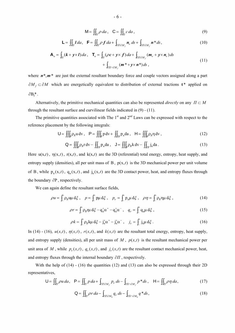
- 6 -

, ,Π Π

da c daρ= =∫∫ ∫∫M C (9)

, ,f fΠ Π Π\ M Π\ M

da da ds dsνρ∂ ∂ ∂ ∂

= = + +∫∫ ∫∫ ∫ ∫l f n n*L F (10)

o o( ) , ( ) ( )

( ) ,f

f

Π Π Π\ M

Π M

da da ds

ds

ν νρ∂ ∂

∂ ∩∂

= + × = + × + + ×

+ + ×

∫ ∫ ∫

∫

k y l c y f m y n

m* y n*

A T (11)

where ,n* m* are just the external resultant boundary force and couple vectors assigned along a part

fM M∂ ⊂ ∂ which are energetically equivalent to distribution of external tractions *t applied on

fB *∂ .

Alternatively, the primitive mechanical quantities can also be represented directly on any Π M⊂

through the resultant surface and curvilinear fields indicated in (9) - (11).

The primitive quantities associated with The 1st and 2nd Laws can be expressed with respect to the

reference placement by the following integrals:

nP P P Pu dv , pdv p da , dv ,R R∂

= ρ = + = ρ η∫∫∫ ∫∫∫ ∫∫ ∫∫∫U P H (12)

n nP P P Pr dv p da , k dv j da .R R∂ ∂

= ρ − = ρ −∫∫∫ ∫∫ ∫∫∫ ∫∫Q J (13)

Here u(x, )t , (x, )tη , r(x, )t , and k(x, )t are the 3D (referential) total energy, entropy, heat supply, and

entropy supply (densities), all per unit mass of B , p(x, )t is the 3D mechanical power per unit volume

of B , while np (x, )t , nq (x, )t , and nj (x, )t are the 3D contact power, heat, and entropy fluxes through

the boundary P∂ , respectively.

We can again define the resultant surface fields,

nu d , p d , p d , d ,R Ru p pνρ ξ ξ ξ ρη ξ+ + + +

− − − −= ρ μ = μ = μ = ρ ημ∫ ∫ ∫ ∫ (14)

n n nr d q q , q d ,Rr qνρ ξ ξ+ ++ + + −

− −= ρ μ − α − α = μ∫ ∫ (15)

n n nk d j j , j d .Rk jνρ ξ ξ+ ++ + + −

− −= ρ μ − α − α = μ∫ ∫ (16)

In (14) - (16), ( , )u x t , ( , )x tη , ( , )r x t , and ( , )k x t are the resultant total energy, entropy, heat supply,

and entropy supply (densities), all per unit mass of M , ( , )p x t is the resultant mechanical power per

unit area of M , while ( , )p x tν , ( , )q x tν , and ( , )j x tν are the resultant contact mechanical power, heat,

and entropy fluxes through the internal boundary Π∂ , respectively.

With the help of (14) - (16) the quantities (12) and (13) can also be expressed through their 2D

representatives,

, * , ,f fΠ Π Π\ M Π M Π

u da p da p ds p ds daνρ ρη∂ ∂ ∂ ∩∂

= = + − =∫∫ ∫∫ ∫ ∫ ∫∫U P H (17)

* ,h hΠ Π\ M Π M

r da q ds q dsνρ∂ ∂ ∂ ∩∂

= − −∫∫ ∫ ∫Q (18)

- 7 -

* ,h hΠ Π\ M Π M

k da j ds j dsνρ∂ ∂ ∂ ∩∂

= − −∫∫ ∫ ∫J (19)

where *p is the external, resultant boundary power flux assigned along fM∂ , while *q and *j are

the external, resultant boundary heat and entropy fluxes given along a part hM M∂ ⊂ ∂ which are

thermally equivalent to distributions of 3D heat q* and entropy j* fluxes assigned on B* B*h∂ ⊂ ∂ .

Alternatively, the primitive quantities (12) - (13) can also be represented directly on any Π M⊂

through the surface and curvilinear fields as indicated in (17) - (19).

By the Cauchy postulate extended to the 2D thermal fields, the contact surface quantities νn , νm ,

qν , and jν can be represented through the respective surface stress resultant ( , ) xx t V T M∈ ⊗N and

stress couple ( , ) xx t V T M∈ ⊗M tensors of the 1st Piola-Kirchhoff type, as well as the respective

referential heat ( , ) xx t T M∈q and entropy ( , ) xx t T M∈j flux vectors according to

, , , , .p q jν ν ν ν ν= = = ⋅ = ⋅ = ⋅n Nν m Mν p ν q ν j ν (20)

In these relations xT M∈ν is the unit vector externally normal to Π∂ , and xT M is the 2D vector

space tangent to M at x M∈ .

In what follows we assume, as is usual in solid mechanics, that mass is not produced during the

process, 0≡C . Hence, the balance of mass (1)1 is identically satisfied.

If time derivatives of the set functions o( , ) , ( , ), ( , )t t tUL AP P P , ( , )tP P , and ( , )tH P exist for all

t T∈ we can write

2 2 2 2 22 2 2 2 21 1 1 1 11 1 1 1 1

o o| , | , | , | , | .t t t t tt t t t t

t t t t tt t t t tdt dt dt dt dt= = = = =∫ ∫ ∫ ∫ ∫U U P P H HL L A A (21)

Then using the 2D representations (9) - (19), we obtain

, ( ) ( ) ,Π Π Π Π

d dda da da dadt dt

= + × = + × + ×∫∫ ∫∫ ∫∫ ∫∫l l k y l k y l y l (22)

Π Π Π Π Π Π

d d du da u da , p da p da , da da ,dt dt dt

ρ ρ ρη ρη= = =∫∫ ∫∫ ∫∫ ∫∫ ∫∫ ∫∫ (23)

and the four remaining laws of mechanics and thermodynamics for the shell-like body become

( ) ,f fΠ Π\ M Π\ M

da ds dsνρ∂ ∂ ∂ ∂

− + + =∫∫ ∫ ∫ 0f l n n* (24)

{ ( ) ( )}

( ) ( ) ,f f

Π

Π\ M Π M

da

ds dsν ν

ρ ρ

∂ ∂ ∂ ∩∂

− + × + × −

+ + × + + × =

∫∫∫ ∫ 0

c k y l y f l

m y n m* y n* (25)

( ) *

* 0,f h

h h

Π Π\ M Π M

Π Π\ M Π M

u p da p ds p ds

r da q ds q ds

ν

ν

ρ

ρ

∂ ∂ ∂ ∩∂

∂ ∂ ∂ ∩∂

− − −

− + + =

∫∫ ∫ ∫

∫∫ ∫ ∫ (26)

* 0.h hΠ Π Π\ M Π M

da k da j ds j dsνρη ρ∂ ∂ ∂ ∩∂

− + + ≥∫∫ ∫∫ ∫ ∫ (27)

- 8 -

In what follows we assume that M be a regular geometric surface, so that we exclude any kinks,

branchings and self-intersections (for irregular shells see Chróścielewski et al. 1997, 2004; Makowski

and Pietraszkiewicz 2002; Konopińska and Pietraszkiewicz 2007). We also assume that all surface

fields discussed here are smooth in Π (for thermomechanic processes with jumps at singular surface

curves see Makowski and Pietraszkiewicz 2002; Eremeyev and Pietraszkiewicz 2009, 2010).

Let us apply to (24) - (27) with (20) the surface divergence theorems

, ,Π Π Π Π

ds Div da ds Div da∂ ∂

⋅ = =∫ ∫∫ ∫ ∫∫a ν a Sν S (28)

{ ax[ ( ) ( ) ]} ,T TΠ Π

ds Div Grad Grad da∂

× = × + −∫ ∫∫a Sν a S S a a S (29)

valid for any ( , ) xx t T M∈a and ( , ) xx t V T M∈ ⊗S , where the surface gradient and divergence

operators with respect to x M∈ are defined as in Gurtin and Murdoch (1975), and (ax ) V∈T means

the axial vector of the skew tensor , TV V∈ ⊗ = −T T T , so that (ax )= ×T T 1 , where V V∈ ⊗1 is the

identity tensor. Then, after some transformations we obtain the following four local laws of resultant

shell thermomechanics in the referential (Lagrangian) description valid in any Π M∈ :

, ax ( ) ,T TDiv Divρ ρ+ = + − + = + ×N f l M NF FN c k y l (30)

( ) ( ) 0 ,u p Div r Divρ ρ− + − − =p q (31)

( ) 0 ,k Divρη ρ− − ≥j (32)

where xGrad V T M= ∈ ⊗F y is the surface deformation gradient.

The corresponding dynamic and thermal boundary conditions are

, , * 0 along ,fp M− = − = − ⋅ = ∂0 0n* Nν m* Mν p ν (33)

0 , 0 along ,hq j M− ⋅ = − ⋅ ≥ ∂* q ν * j ν (34)

and the complementary to (33) kinematic boundary conditions are

, along \ .d fM M M− = − = ∂ = ∂ ∂0 0y* y Q* Q (35)

The relations (30) - (35) are formally exact implications of the global laws of continuum

thermodynamics (1), (2), with (21) and 2D representations (9) - (11), (17) - (19), for the shell-like

body represented during motion by the material base surface ( )M t , which in the reference placement

is M .

3. Modified 2D energy balance

Let us analyse in more detail the balance of energy (2)1 and its local 2D form (31).

In 3D continuum mechanics the local form of balance of linear momentum in the referential

description reads

Div ,R R+ρ = ρP b y (36)

- 9 -

where Div means the spatial divergence operator with respect to x B∈ , (x, )tP is the 1st Piola-

Kirchhoff stress tensor, and (x, )tb is the body force vector per unit mass of B . Upon multiplying (36)

by the 3D velocity field (x, )ty , integrating over an arbitrary P B⊂ and using the 3D divergence

theorem, we obtain

P P P P

1( ) Grad ,2R R

dda dv dvdt∂

⋅ + ρ ⋅ − = ρ ⋅∫∫ ∫∫∫ ∫∫∫ ∫∫∫Pn y b y P y y yi (37)

where tr ( )T=A B A Bi for any , V V∈ ⊗A B , and Grad is the spatial gradient operator with respect to

x B∈ . The right-hand side of (37) is K , where ( , )tK P is the kinetic energy, while the left-hand side

means −P S , where ( , )tS P is the stress power.

Let us now use the same approach to the resultant local balance laws (30): multiply (30)1 by a

surface translational velocity ( , )x tυ and (30)2 by a surface angular velocity ( , )x tω of ( )M t , integrate

them over an arbitrary Π M⊂ , use the surface divergence theorems (28) and (29), and finally add

together the two so transformed equations, which leads to

{( ) ( ) } ( )

{ ax ( ) }

{ ( ) } ,

Π ΠT T

Π

Π

ds da

Grad Grad da

da

∂⋅ + ⋅ + ⋅ + ⋅

− − − ⋅ +

= ⋅ + + × ⋅

∫ ∫∫∫∫

∫∫

Nν Mν f c

N NF FN M

l k y l

i i

υ ω υ ω

υ ω ω

υ ω

(38)

where tr ( )T=A D A Di for any , xV T M∈ ⊗A D .

The physical meaning of corresponding terms in (37) and (38) should be the same, only now those

in (38) are expressed through the resultant surface fields alone. The first row of (38) is the mechanical

power performed by ,ν νn m along Π∂ and by ,f c in Π on the respective ,υ ω , the second row

means the stress power performed in Π by ,N M on time rates of appropriately defined 2D shell

strain measures, while the last row should mean the material time derivative of the shell kinetic

energy.

However, neither of those three rows of (38) can be regarded as exact representation on Π and

along Π∂ of the corresponding 3D expressions of (37). In the 2D mechanical power of (38) some part

of the 3D mechanical power of (37) following from stresses P acting on surfaces in B parallel to M

as well as from self-equilibrated distributions across the shell cross section of stresses P , body forces

b and boundary tractions *t is not accounted for. In fact, Pietraszkiewicz et al. (2005) proved

explicitly that the 3D stress power indicated in (37) can be expressed through the 2D stress power

given in (38) plus an additional stress power not expressible through ,N M and not present in (38).

Libai and Simmonds (1983, 1998), by introducing a non-material mass-weighted base surface ( )M t

during the shell motion, were able to represent the last row of (38) in a bulk form similar to that of

kinetic energy of rigid-body motion. But even then some part of 3D kinetic energy of (37) associated

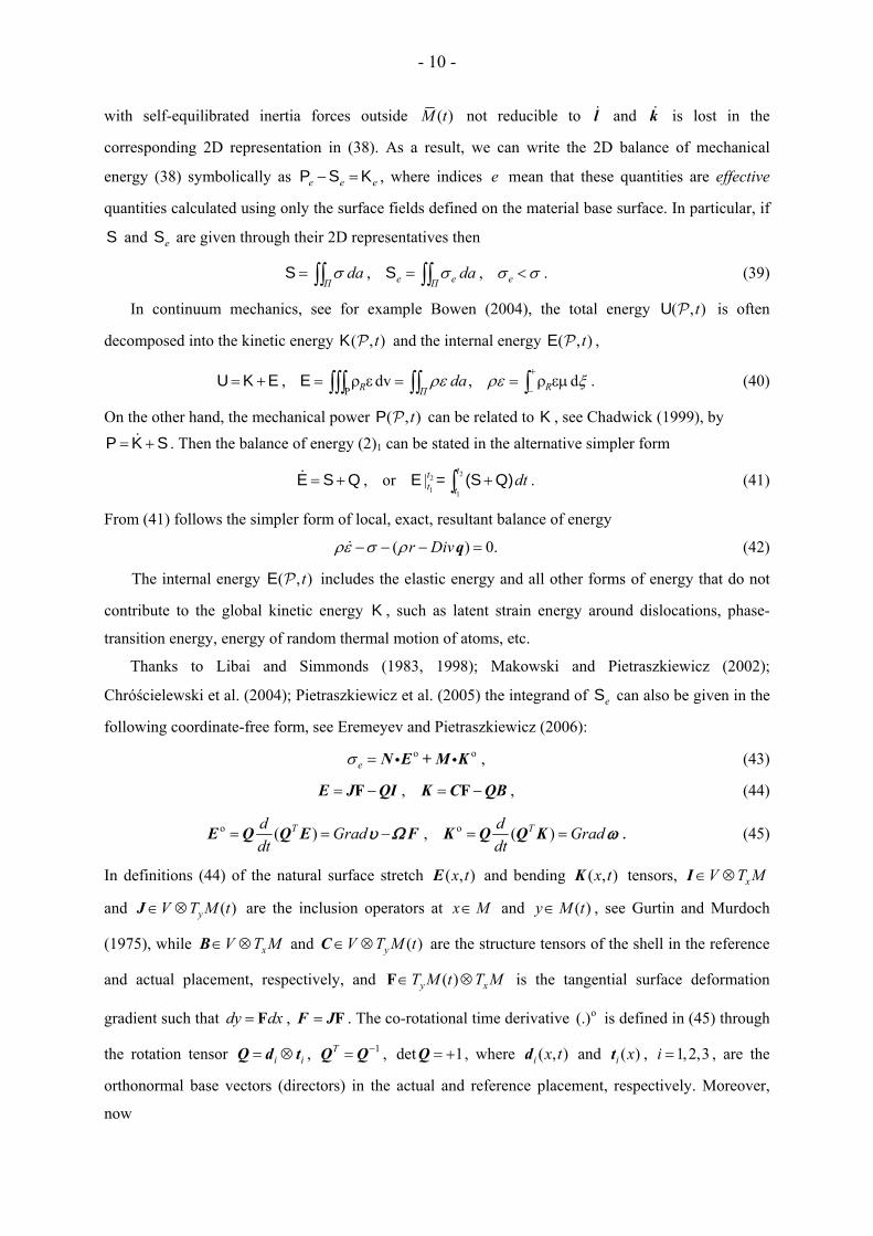
- 10 -

with self-equilibrated inertia forces outside ( )M t not reducible to l and k is lost in the

corresponding 2D representation in (38). As a result, we can write the 2D balance of mechanical

energy (38) symbolically as e e e− =P S K , where indices e mean that these quantities are effective

quantities calculated using only the surface fields defined on the material base surface. In particular, if

S and eS are given through their 2D representatives then

, , .e e eΠ Πda daσ σ σ σ= = <∫∫ ∫∫S S (39)

In continuum mechanics, see for example Bowen (2004), the total energy ( , )tU P is often

decomposed into the kinetic energy ( , )tK P and the internal energy ( , )tE P ,

P

, dv , d .R RΠdaρε ρε ξ

+

−= + = ρ ε = = ρ εμ∫∫∫ ∫∫ ∫U K E E (40)

On the other hand, the mechanical power ( , )tP P can be related to K , see Chadwick (1999), by = +P K S . Then the balance of energy (2)1 can be stated in the alternative simpler form

221 1

, or | .tt

t tdt= + +∫E S Q E = (S Q) (41)

From (41) follows the simpler form of local, exact, resultant balance of energy

( ) 0.r Divρε σ ρ− − − =q (42)

The internal energy ( , )tE P includes the elastic energy and all other forms of energy that do not

contribute to the global kinetic energy K , such as latent strain energy around dislocations, phase-

transition energy, energy of random thermal motion of atoms, etc.

Thanks to Libai and Simmonds (1983, 1998); Makowski and Pietraszkiewicz (2002);

Chróścielewski et al. (2004); Pietraszkiewicz et al. (2005) the integrand of eS can also be given in the

following coordinate-free form, see Eremeyev and Pietraszkiewicz (2006):

o o ,eσ = N E + M Ki i (43)

, ,= − = −F FE J QI K C QB (44)

o o( ) , ( )T Td dGrad Graddt dt

= = − = =E Q Q E F K Q Q Kυ Ω ω (45)

In definitions (44) of the natural surface stretch ( , )x tE and bending ( , )x tK tensors, xV T M∈ ⊗I

and ( )yV T M t∈ ⊗J are the inclusion operators at x M∈ and ( )y M t∈ , see Gurtin and Murdoch

(1975), while xV T M∈ ⊗B and ( )yV T M t∈ ⊗C are the structure tensors of the shell in the reference

and actual placement, respectively, and ( )y xT M t T M∈ ⊗F is the tangential surface deformation

gradient such that dy dx= F , = FF J . The co-rotational time derivative o(.) is defined in (45) through

the rotation tensor i i= ⊗Q d t , 1T −=Q Q , det 1= +Q , where ( , )i x td and ( )i xt , 1,2,3i = , are the

orthonormal base vectors (directors) in the actual and reference placement, respectively. Moreover,

now

- 11 -

, , ax ( ) , ,T= − = = = = ×1u y x y u QQυ ω Ω ω (46)

where ( , )x tu is the surface translation vector and ( , )x tQ is the surface rotation tensor. The fields u

(or y ) and Q are independent kinematic variables of the shell motion.

Let us introduce an additional stress power ( , )tW P of the shell-like body, called here the

interstitial working after Dunn and Serrin (1985), such that e= +S S W . The quantity W takes into

account that part of the 3D stress power which is lost in defining eS in (43) only through the surface

fields. For any Π M⊂ the interstitial working may be represented locally as

,Π Π

w ds Div daν∂= =∫ ∫∫ wW (47)

where ( , )w x tν is the surface contact interstitial working (density) and ( , ) xx t T M∈w is the

corresponding surface interstitial working flux vector such that wν = ⋅w ν , so that now

e Divσ σ= + w . Then the local, resultant balance of energy (42) is modified into

o o( ) ( ) 0 .Div r Divρε ρ− + − − =N E + M K w qi i (48)

The resultant equation (48) can now be regarded as an exact implication of the global 3D balance

of energy (41).

The quantity aP , also called the interstitial working, was first introduced into shell theory by

Makowski and Pietraszkiewicz (2002) to correct the effective mechanical power eP of (38) into

e a= +P P P to be used in the balance of energy (2)1. The aP necessarily consisted of three terms

defined in Π , along fΠ \ M∂ ∂ , and along fΠ M∂ ∩∂ . This considerably complicated refined forms of

The 1st and 2nd Laws for shells.

4. Modified 2D entropy inequality

The local resultant entropy inequality in the form (32) is entirely decoupled from other local

resultant balance laws (30) and (48).

In continuum thermodynamics coupling of The 2nd Law (2)2 with other balance laws (1)2,3 and

with (2)1 is achieved by introducing the absolute 3D temperature field θ(x, ) 0t > , through which the

fields k(x, )t and nj (x, )t in (13)2 are related to those r(x, )t and nq (x, )t in (13)1 . In rational

thermomechanics these relations are taken as k r/= θ and nj /= ⋅ θq n . The 3D entropy inequality in

the form

RP P P

rη Rdv dv da∂

⋅ρ ≥ ρ −

θ θ∫∫∫ ∫∫∫ ∫∫q n (49)

is usually called the Clausius-Duhem inequality, see Truesdell and Toupin (1960); Truesdell (1984).

- 12 -

It is recognised in the literature that the inequality (49) is appropriate for a wide class of

homogeneous materials, but is still insufficient in modelling for example multicomponent continua or

continua with non-mechanical (e.g. electromagnetic) fields, see Wilmanski (2008). For other forms of

relations between n nk, j , r,q and θ leading to other than (49) forms of The 2nd Law see for example

Müller (1967); Gurtin and Williams (1967); Green and Laws (1972); Müller and Ruggeri (1998).

Since θ appears in denominator of (49), during the 3D-to-2D reduction procedure it is not

convenient to use either the resultant surface temperature dξ+

−θμ∫ or the thickness-averaged surface

temperature /d hξ+

−θμ∫ . But some kind of mean referential temperature has to be defined on M and

taken outside the through-the-thickness integration in (49), otherwise a reasonable 2D representation

of J through the surface and boundary heat fields cannot be achieved.

Three different 2D temperature fields appear naturally in shell thermodynamics: a reference

temperature associated with the base surface, and temperatures of the upper and lower shell faces.

Postulating some reasonable relations between the three surface temperatures one can reduce the

number of independent 2D temperature fields to two or to one, whichever is appropriate. In particular,

Murdoch (1976) proposed to use only one common temperature field associated with M , an this

approach has recently been used by Eremeyev and Pietraszkiewicz (2009). Temperatures of the upper

and lower shell faces as independent fields were used by Zhilin (1976); Eremeyev and Zubov (2008),

while Naghdi (1972); Green and Naghdi (1979) used the thickness-averaged temperature and its

derivative in the transverse normal direction evaluated on M as independent fields. Any such

proposal leads to a slightly different structure of the thermodynamic initial-boundary value problem

for shells. In particular, for two independent 2D temperature fields one needs two independent 2D

energy balance equations. Since the shell thermodynamic theories mentioned above are not the

resultant ones, they introduce an indefinable error into the 2D energy balance and entropy inequality.

Recently Eremeyev and Pietraszkiewicz (2010) developed the resultant, thermomechanic, quasistatic

model of phase transitions in shells, where the referential mean temperature and its deviation

suggested by Murdoch (1976a) were used.

In this paper we define the surface mean referential temperature ( , )x tθ by

+ + + +

1 1 1 1 1 1 1 1 1 1 1 1 1 1, , ,2 θ θ θ 2 θ θ θ 2 θ θθ θ θ− − − −

⎛ ⎞ ⎛ ⎞ ⎛ ⎞= + = − − = + −⎜ ⎟ ⎜ ⎟ ⎜ ⎟

⎝ ⎠ ⎝ ⎠ ⎝ ⎠ (50)

where θ+ and θ− are values of temperature on the upper and lower shell faces M + and M − ,

respectively. The use of so defined θ itself does not introduce any approximation. Then the through-

the-thickness integration in (49) with (50) allows one to represent the Clausius-Duhem inequality in

the resultant form

- 13 -

2

1 1

* 0 ,*h

Π

Π M

r s Div Div da

qq* s s dsνν

ρη ρθ θ θ

θ θ∂ ∩∂

⎧ ⎫⎛ ⎞− + + − ⋅ +⎨ ⎬⎜ ⎟⎝ ⎠⎩ ⎭

⎧ ⎫⎛ ⎞+ + − + ≥⎨ ⎬⎜ ⎟⎝ ⎠⎩ ⎭

∫∫

∫

q q g s (51)

where

( )_, r ,x RGrad T M r dθ ρ ξ

+ + + − −+ −= ∈ = ρ μ − ⋅ α + ⋅ α∫ q n q ng (52)

( )+

1 1 1 1 1r ,2 θ θRs dρ ξ

θ+ + + − −

+ −−−

⎛ ⎞⎛ ⎞= − ρ μ + − ⋅ α − ⋅ α⎜ ⎟⎜ ⎟θ⎝ ⎠ ⎝ ⎠∫ q n q n (53)

1 1* , * ,q d s dν νξ ξθ

+ +

− −

⎛ ⎞= ⋅ = ⋅ μ = ⋅ = − ⋅ μ⎜ ⎟θ⎝ ⎠∫ ∫q n q nq ν s ν (54)

1 1* * * , * * * ,*q d s dξ ξθ

+ +

− −

⎛ ⎞= ⋅ = ⋅ μ = ⋅ = − ⋅ μ⎜ ⎟∗θ⎝ ⎠∫ ∫q n q nq* ν s* ν (55)

and the geometric parameters , , *± ±μ, α n n are given by Konopińska and Pietraszkiewicz (2007),

Appendix (A.15) – (A.17).

With definitions (52) - (55), the relations between the resultant fields appearing in (31), (32) and

(34) become

, , .rk sθ θ θ

= + = + = +q q*j s j* s* (56)

The extra surface fields , ,s s s* in (56) take into account the extra surface heat and entropy supplies

following from non-uniform distribution across the shell thickness of the temperature field θ , which

now enters (51) only through its values +θ and −θ on the upper and lower shell faces. Presence of the

extra fields in (51) assures that the resultant form of Clausius–Duhem inequality (51) still remains an

exact implication of the 3D principle (49) .

With usual continuity assumptions the local form of (51) is

21 1( ) 0 in r Div s Div Π M ,ρη ρ ρθ θ

− − − + − ⋅ ≥ ⊂q s q g (57)

* * 0 along .* h

q s Mθ θ

⎛ ⎞+ − + ⋅ ≥ ∂⎜ ⎟⎝ ⎠q s ν (58)

The inequality (57) may be transformed into another form more convenient for discussing 2D

constitutive equations. Let us solve the exact, resultant balance of energy (48) for r Div− q and use

the result in (57), which gives

o o 1( ) 0 in .Div s Div Π Mρθη ρε ρθ θθ

− + + + − − ⋅ + ≥ ⊂N E M K w q g si i (59)

Then we introduce the surface free energy (density) ( , )x tψ by ψ ε θη= − , so that θη ε ψ θη− = − − ,

and (59) takes the final form

- 14 -

o o 1 0 in Div s Div Π M .ρψ ρθη ρθ θθ

− − + + + − − ⋅ + ≥ ⊂N E M K w q g si i (60)

The local, resultant 2D entropy inequality (60) can now be regarded as an exact implication of the

global Clausius–Duhem inequality (49) as well.

5. Restrictions on the form of constitutive equations

The starting points of our shell thermomechanics have been the classical 3D Cauchy continuum

and the 3D Clausius–Duhem inequality. But our resultant thermomechanic shell relations are far from

being the classical ones:

1. The kinematic structure of the resultant shell theory is that of the Cosserat (1909) surface, with

( , )x ty and ( , )x tQ as independent kinematic field variables of the shell motion.

2. The thermodynamic structure of our refined, resultant laws (48) and (60) does not remind that

of 3D rational thermomechanics developed in Truesdell (1975, 1984). In particular, our 2D

laws of thermomechanics contain the extra surface scalar field ( , )s x t and divergences of the

additional surface vector fields ( , )x tw and ( , )x ts which are not present in corresponding 3D

laws. Our exact, local, resultant balance laws (30), (48) and the inequality (60) are expressed through 16

fields, which together form the shell thermomechanic process over the domain M T× . Different

groups of fields play different roles in the process. The fields , ,θy Q constitute the basic thermo-

kinematic independent field variables of the initial-boundary value problem of shell thermomechanics.

That only seven scalar fields can be taken as independent field variables here follows from the fact

that there are only seven scalar resultant field equations (30) and (48) to determine them. The fields

, , , , , , ,sε ηN M q w s have to be specified by appropriate material constitutive equations and the fields

,l k by appropriate kinetic constitutive equations. When all the fields above are settled, the fields

, , rf c are supposed to be adjusted so as to satisfy the 2D balance equations (30) and (48). Every such

process is called an admissible thermomechanic process; it is completely determined by the evolution

of deformation and temperature of the shell base surface.

In the resultant shell thermomechanics specific forms of the constitutive equations can be

established by two main approaches. The direct approach consists in developing, for a restricted class

of shell-like bodies, a general structure of 2D constitutive equations satisfying some reasonable

physical and mathematical requirements. Then one has to devise a suitable sets of experiments from

which the appropriate material constants or functions entering the constitutive equations can be

established. In the derived or deductive approach one has to devise suitable mathematical methods

allowing one to deduce the 2D constitutive equations for shells as an exact, asymptotic of otherwise

- 15 -

rational consequence of a given set of corresponding 3D constitutive equations of the parent theory. In

the present paper the constitutive equations are developed by the direct approach.

General requirements that the material constitutive equations of our resultant shell

thermomechanics must obey are analogous to those of 3D rational thermomechanics formulated by

Truesdell and Toupin (1960), section 293. These are briefly: 1) consistency, 2) coordinate invariance,

3) well posedness, 4) material frame-indifference, 5) material symmetry, and 6) equipresence.

Additional quite general requirements were proposed in Truesdell and Noll (1965): 7) determinism, 8)

local action, and 9) fading memory. But in the literature one can find many other specific requirements

which define particular classes of material behaviour, such as for example hyper- and hypoelasticity,

viscosity, incompressibility, inextensibility in some direction, slow motions, small deformations, etc.

Either of these requirements can be used to define particular classes of shell constitutive behaviour as

well.

Let us introduce the referential shell stress measures ( , )x tN and ( , )x tM with corresponding

referential shell strain measures ( , )x tE and ( , )x tK defined by

, , , ,T T T T T T= = = = − = = −N M E F K FQ N Q M Q E Q J I Q K Q C B (61)

so that the local 2D inequality (60) becomes

1 0 in Div s Div Π M .ρψ ρθη ρθ θθ

− − + + + − − ⋅ + ≥ ⊂N E M K w q g si i (62)

If , ,θy Q are taken as the independent field variables, then from the requirement of determinism

the 2D thermomechanic response described by the fields ( , , , , , , , , , )sΣ ε η= N M q w s l k at the shell

particle, whose position in the reference placement is x M∈ , can mathematically be defined by the

response functionals

0ˆ( , ) ( , ), ( , ), ( , ); , ( ) ,t t tx t z z z z zτΣ Σ τ τ θ τ∞= ⎡ ⎤= ⎣ ⎦y Q B (63)

where history ( , ) ( , )t x x tφ τ φ τ≡ − up to the present time t of any field ( , )x tφ in (63) is defined for all

[0, )τ ∈ +∞ , and where z M∈ is any other place than x on M . The explicit dependence of the right-

hand side of (63) on z and on the referential structure tensor ( )zB indicates that thermomechanic

properties at x M∈ may depend also on properties of other shell particles in Π M⊂ thus allowing

for material inhomogeneous and non-uniform behaviour, in general.

In the special case of (63), which we wish to investigate in more detail as an example, we allow

the fields Σ to depend on ty , tQ , and tθ only locally through the first time derivatives at 0τ = and

locally through the first surface gradients at x . Then the corresponding constitutive assumption would

be

ˆ( , ) , , , , , ; , ( ) .x t x xΣ Σ θκ ⎡ ⎤= ⎣ ⎦E K E K g B (64)

- 16 -

Any function in Σ̂ κ is called the response or constitutive function and is assumed to be differentiable

with respect to the indicated fields as many times as required. The index κ in Σ̂ κ indicates that the

form of each response function depends on the choice of the reference placement.

5.1. Viscous shells with heat conduction

The shell-like body described by the 2D response functions (64) is usually called a viscous shell

with heat conduction. But in our 2D entropy inequality (62) there is the non-standard vector field

( , )x tw which within 3D continuum mechanics allows for modelling the material behaviour also with

mechanical longer-range spatial interactions at x M∈ , see Dunn and Serrin (1985); Dunn (1986).

Additionally, the presence of Divθ s in (62) suggests that also the thermal longer-range spatial

interactions at x M⊂ may be accounted for in the resultant shell thermomechanics. Hence, the more

appropriate non-classical constitutive assumption for the viscous shell with heat conduction

compatible with (62) is

[ ]ˆ( , ) ; , ( ) , ( , , , , , , , , ) ,x t x x Grad GradΣ Σ Λ Λ θκ= = E K E K E KB g G (65)

where Tx xGrad T M T M= = ∈ ⊗G g G .

The thermomechanic process, in which the fields , ,θE K are constant in space and time, is usually

called the equilibrium process. The equilibrium response functions of the shell stress measures

,E EN M are defined by

[ ] [ ]0 0

0

ˆ ˆ; , ( ) , ; , ( ) ,( , , , , , , , , ) .

E E E Ex x x xΛ ΛΛ θ

κ κ= =

=

N N M ME K 0 0 0 0 0 0

B B (66)

Then the dynamic, dissipative parts of the response functions of the shell stress measures are such that

[ ] [ ]ˆ ˆ; , ( ) , ; , ( ) ,

, .

D D D D

E D E D

x x x xΛ Λκ κ= =

= + = +

N N M M

N N N M M M

B B (67)

According to Coleman and Noll (1963), in 3D rational thermodynamics the Clausius–Duhem

inequality plays the role of a restriction placed on allowable forms of the response functions. The

functions must be so chosen as to satisfy the inequality in every smooth thermomechanic process

compatible with the 3D balance equations.

To reveal the restrictions placed on the shell constitutive equations (65) by our resultant entropy

inequality, let us just introduce (65) into the inequality (62) to obtain

( , ) ( , ) ( , ) ,

, , , ,

1, 0 .

Grad GradGrad Grad

s Div Div

θρψ ρψ ρη ρψ θ ρψ

ρψ ρψ ρψ ρψ

ρψ ρθ θθ

− + − − + − ⋅

− − − −

− − − ⋅ + + ≥

Ε K

E K E K

N E M K

E K E Kg

G

g

G q g w s

i i

i i i i

i

(68)

- 17 -

Any deformation–temperature path can be realised in a thermomechanic process, so that values of

Λ and Λ can be chosen arbitrarily. Since the left-hand side of (68) depends on Λ linearly, in order

to satisfy (68) the coefficients in front of time rates of variables must vanish,

, , , , , , , , , , , , , .Grad Gradθη ψ ψ ψ ψ ψ ψ ψ= − = = = = = =E K E K0 0 0 0 0 0g G (69)

These relations imply that [ ]ˆ , , ; , ( )x xψ ψ θκ= E K B , and by (69)1 and definition of ψ the same

structure should have the response functions ε̂ κ and η̂κ .

With (69) the inequality (68) reduces to

1( , ) ( , ) 0 .s Div Divρψ ρψ ρθ θθ

− + − − − ⋅ + + ≥Ε KN E M K q g w si i (70)

Since 0ρ > and 0θ > , from (70) it follows that the field s is required to be non-positive,

0s ≤ . Please also note that in (70), N and M still depend on Λ , while ,ψ E and ,ψ K depend only on

, ,θE K . If the decompositions (66) and (67) are used in (70), the following constitutive equations for

the equilibrium part of the shell stress measures are obtained:

[ ] [ ]ˆ ˆ, , , ; , ( ) , , , , ; , ( ) .E Ex x x xψ θ ψ θκ κ= =E KN E K M E KB B (71)

Let us now apply the chain rule to the surface vector fields w and s , which allows one to expand

(70) with (71) into

2

1 1 1, , , ,

1 1 1tr , , tr , , tr , ,

1 1tr , , tr , ,

D D

Grad Grad Grad G

s

Grad Grad Grad

Grad

θ θρθθ θ θ

θ θ θ

θ θ

⎛ ⎞ ⎛ ⎞+ − − − − ⋅ + +⎜ ⎟ ⎜ ⎟⎝ ⎠ ⎝ ⎠

⎡ ⎤ ⎡ ⎤ ⎡ ⎤⎛ ⎞ ⎛ ⎞ ⎛ ⎞+ + + + + +⎜ ⎟ ⎜ ⎟ ⎜ ⎟⎢ ⎥ ⎢ ⎥ ⎢ ⎥⎝ ⎠ ⎝ ⎠ ⎝ ⎠⎣ ⎦ ⎣ ⎦ ⎣ ⎦⎡ ⎤⎛ ⎞+ + ◊ + +⎜ ⎟⎢ ⎥⎝ ⎠⎣ ⎦

E E K K

E E K

N E M K

E K

E

g g

G G

q w s g w s G

w s G w s w s

w s w s

i i i

2 0 ,rad Grad⎡ ⎤⎛ ⎞◊ ≥⎜ ⎟⎢ ⎥⎝ ⎠⎣ ⎦K K

(72)

where for two 3rd-order surface tensors ,Λ Δ and for two 4th-order surface tensors ,Φ Ψ the 2nd-order

surface tensors Λ Δ and ◊Φ Ψ are defined such that in Cartesian components associated with xT M ,

( ) , ( ) , , 1,2.i i i iαβ α λ λβ αβ α λμ λμβΛ Δ Φ Ψ α β= ◊ = =Λ Δ Φ Ψ (73)

Let us remind that the interstitial working vector w is of entirely mechanical origins. Hence, we

may additionally assume that [ ]ˆ , , , ; , ( )Grad Grad x xκ= E K E Kw w B , so that , , .θ = = 0gw w Similarly,

the extra surface field s is of entirely thermal origins and we may additionally assume that

[ ]ˆ , , ; , ( )x xθκ=s s g G B , so that , , , ,Grad Grad= = = =E K E K 0s s s s . With these additional assumptions the

inequality (72) reduces to

( )

( ) ( ) ( ) ( )2 2

1 1 1, , tr ,

tr , tr , tr , tr , 0 .

D D

Grad Grad

s Grad

Grad Grad Grad Grad

θρθθ θ θ

⎛ ⎞+ − − − ⋅ + + ⎜ ⎟⎝ ⎠

+ + + ◊ + ◊ ≥E K E K

N E M K

E K E K

g Gq s g s G s G

w w w w

i i i (74)

- 18 -

5.2. Thermoelastic shells

An important special case of viscous shells with heat conduction are thermoelastic shells, for

which the constitutive functions in (65)1 do not depend on ,E K . In this case the refined entropy

inequality takes the form (68), only now without terms containing ,ψ E and ,ψ K . To satisfy it we

should have

, , , , , , , ,Grad Gradψ ψ ψ ψ= = = =E K0 0 0 0g G (75)

so that also in this case [ ]ˆ , , ; , ( )x xψ ψ θκ= E K B , with the same structure of ε̂ κ and η̂κ . As a result,

the constitutive equations for N , M , and η of the thermoelastic shells are

, , , , , .θρψ ρψ η ψ= = = −E KN M (76)

With the constitutive equations (76) the reduced form of our entropy inequality becomes

2

1 1 1 1, , , , tr , ,

1 1tr , , tr , ,

1 1tr , , tr , ,Grad Grad Grad Grad

s Grad

Grad Grad

Grad

θ θρθθ θ θ θ

θ θ

θ θ

⎡ ⎤⎛ ⎞ ⎛ ⎞ ⎛ ⎞− − − − ⋅ + + + +⎜ ⎟ ⎜ ⎟ ⎜ ⎟⎢ ⎥⎝ ⎠ ⎝ ⎠ ⎝ ⎠⎣ ⎦⎡ ⎤ ⎡ ⎤⎛ ⎞ ⎛ ⎞+ + + +⎜ ⎟ ⎜ ⎟⎢ ⎥ ⎢ ⎥⎝ ⎠ ⎝ ⎠⎣ ⎦ ⎣ ⎦⎡ ⎤⎛ ⎞ ⎛ ⎞+ + ◊ + + ◊⎜ ⎟ ⎜ ⎟⎢ ⎥⎝ ⎠ ⎝ ⎠⎣ ⎦

E E K K

E E K K

E K

E

g g G Gq w s g w s G w s G

w s w s

w s w s

i

2 0 .Grad⎡ ⎤≥⎢ ⎥

⎣ ⎦K

(77)

If again ˆ κw in (77) is assumed not to depend on ,θ g and ˆκs on , , ,Grad GradE K E K then the

inequality (77) reduces further to

( )

( ) ( ) ( ) ( )2 2

1 1 1, , tr ,

tr , tr , tr , tr , 0 .Grad Grad

s Grad

Grad Grad Grad Grad

θρθθ θ θ

⎛ ⎞− − − ⋅ + + ⎜ ⎟⎝ ⎠

+ + + ◊ + ◊ ≥E K E KE K E K

g Gq s g s G s G

w w w w

i (78)

In both cases of viscous shells with heat conduction and of thermoelastic shells the reduced

entropy inequalities (74) and (78) still put some constraints on allowable forms of ˆ κw and ˆκs , but we

postpone their further discussion here. But the main message following from (74) and (78) is that our

refined, resultant entropy inequality does allow the constitutive equations of the both types of shells to

depend on Grad E , Grad K , and G indeed. However, before fully revealing such an explicit

dependence much research has still to be done.

5.3. Kinetic constitutive equations

The simple relation R= ρl y used in (4) and (37) is in fact a kind of kinetic 3D constitutive

equation for the 3D kinetic momentum vector (x, )tl introduced into the Cauchy continuum mechanics

by the Newton law.

- 19 -

In the resultant shell thermomechanics it is not apparent how the resultant linear momentum

( , )x tl and angular momentum ( , )x tk vector fields should be related to the 2D translational and

angular velocities υ and ω as well as to other kinematic and thermal surface fields. Since the fields

,l k do not enter into our refined resultant entropy inequality (59), it does not place any

thermodynamic restrictions on their functional forms. We propose below some heuristic arguments,

extending those give in Chróścielewski et al. (2004), how the 2D kinetic constitutive equations can be

constructed within the classes of shell models discussed in subsections 5.1 and 5.2.

Since l and k are of entirely mechanical origins, the 2D constitutive equations for them may be

postulated in the reduced form

ˆ , , , , , , , ; , ( ) ,

ˆ , , , , , , , ; , ( ) .

Grad Grad x x

Grad Grad x x

κ

κ

⎡ ⎤= ⎣ ⎦⎡ ⎤= ⎣ ⎦

E K E K E K

E K E K E K

l l B

k k B

υ ω

υ ω (79)

In analogy to the 3D case, it is reasonable to assume that the constitutive functions κ̂l and ˆκk are

linear functions of ,υ ω ,

1 2 3 4, .= + = +l J J k J Jυ ω υ ω (80)

Here A V V∈ ⊗J , 1,2,3,4A = , are tensor functions of , , , , ,Grad GradE K E K E K , in general.

If the tensors AJ satisfy the symmetry conditions

1 1 2 3 4 4, , ,T T TJ = J J = J J = J (81)

we may expect existence of the 2D kinetic energy density ,x tκ( ) per unit surface of M , which is the

quadratic function of ,υ ω ,

( )1 2 3 41 .2

κ = ⋅ + ⋅ + ⋅ + ⋅J J J Jυ υ υ ω ω υ ω ω (82)

The function κ may serve as potential for ,l k , so that (80) can be found from κ according to

, , , .κ κ= =l kυ ω (83)

The tensors AJ may be taken to be quite complex functions of all their arguments, in general. But

because of mechanical origins of l and k we may additionally assume that ( , , )A A ρ= E KJ J . With

such AJ the kinetic constitutive equations (80) was proposed by Chróścielewski et al. (2004).

Particularly appealing forms of (80) appear when, in analogy to the rigid-body motion, the AJ are

assumed to be

1 2 3 3 4 4, , ,T T Tρ ρ ρ= = = =1J J J QI Q J QI Q (84)

where 3I and 4I are constant inertia tensors which explicit definitions depend on specific internal

structure of the shell across the thickness. In this case, according to (83) we obtain

3 3 4, .T T T Tρ ρ ρ ρ= + = +l QI Q k QI Q QI Qυ ω (85)

- 20 -

The kinetic constitutive equations (85) were used, for example, by Altenbach and Zhilin

(1988); Eremeyev and Zubov (2008).

In many contemporary papers on shell dynamics the inertia tensors are taken in the ultimately

simple forms leading to

1 2 3 4, , ,Iρ ρ= = = =1 0 1J J J J (86)

where I is the geometric moment of inertia of the shell cross section. The simplest 2D kinetic

constitutive equations , Iρ ρ= =l kυ ω following from (83) with (86) were applied for example by

Zhilin (1976); Libai and Simmonds (1983, 1998); Chróścielewski et al. (2004).

6. Conclusions

We have derived the new, refined, resultant balance of energy and entropy inequality of the

general shell thermomechanics. The 2D laws may be regarded as exact implications of corresponding

3D laws of rational thermodynamics. The refinement has been achieved by completing the resultant

2D balance of energy, which is initially inaccurate when expressed through the 2D fields alone, with

the interstitial working surface flux vector w . Our refined resultant balance of energy and entropy

inequality contain three non-classical surface fields , ,sw s which play the role of somewhat similar

fields appearing in 3D extended thermodynamics, see Müller and Ruggeri (1998).

We have briefly analysed restrictions imposed by our refined resultant entropy inequality on the

2D constitutive equations of viscous shells with heat conduction and of thermoelastic shells. Applying

the procedure of Coleman and Noll (1963), it has been shown that in the both cases our resultant

entropy inequality allows the constitutive equations to depend also on the first surface gradients of

shell strain measures ,E K and on the second surface gradient of the mean surface temperature θ . We

have also provided several novel forms of the 2D kinetic constitutive equations obtained with the help

of heuristic arguments.

More definite properties of the non-classical fields , ,sw s as well as reduced explicit forms of the

constitutive equations following from requirements of material frame-indifference and material

symmetry for these types of shells should be discussed separately. Due to the non-classical form of the

reduced inequalities (74) and (78) as well as a number of independent fields in the constitutive

equations (65), it is natural to expect that the corresponding analyses be quite involved.

Acknowledgements The research reported in this paper was supported by the Polish Ministry of Science and Education under grant No N 501 0073 33.

- 21 -

References 1) Altenbach, H., Zhilin, P.A., 1988. Theory of elastic simple shells. Advances of Mechanics 11, 107-148 (in

Russian).

2) Badur, J., 2009. Development of Notion of Energy (in Polish), Wydawnictwo IMP PAN, Gdańsk.

3) Bowen, R.M., 2004. Introduction to Continuum Mechanics for Engineers. Plenum Press.

4) Chadwick, P., 1999. Continuum Mechanics. Dover Publ., Mineola.

5) Chróścielewski, J., Makowski, J., Stumpf, H., 1997. Finite-element analysis of smooth, folded and multi-shell structures. Comp. Meth. Appl. Mech. Engng. 41, 1-47.

6) Chróścielewski, J., Makowski, J., Pietraszkiewicz, W., 2004. Statics and Dynamics of Multi-Shells: Non-Linear Theory and the Finite Element Method, Institute of Fundamental Technological Research Press, Warsaw (in Polish).

7) Coleman, B.D., Noll, W., 1963. The thermodynamics of elastic materials with heat conduction and viscosity. Arch. Rational Mech. Anal. 13, 1, 167-178.

8) Cosserat, E., Cosserat, F., 1909. Théorie des Corps Deformables. Hermann et Fils, Paris.

9) Dunn, J.E., 1986. Interstitial working and a non-classical continuum, in: Serrin E. (ed.), New Perspectives in Thermodynamics. Springer-Verlag, Berlin et al, pp. 187-222.

10) Dunn, J.E., Serrin, J., 1985. On the thermodynamics of interstitial working. Arch. Rational Mech. Anal. 85, 95-133.

11) Eremeyev, V.A., Pietraszkiewicz, W., 2006. Local symmetry group in the general theory of elastic shells. J. Elast. 85, 125-152.

12) Eremeyev, V.A., Pietraszkiewicz, W., 2009. Phase transitions in thermoelastic and thermoviscoelastic shells. Arch. Mech., 61, 1, 125-152.

13) Eremeyev, V.A., Pietraszkiewicz, W., 2010. Thermomechanics of shells undergoing phase transitions. J. Mech. Phys. Sol. (in press).

14) Eremeyev, V.A., Zubov, L.M., 2008. Mechanics of Elastic Shells. Nauka, Moscow (in Russian).

15) Green. A.E., Laws. N., 1972. On the entropy production inequality. Arch. Rational Mech. Anal. 45, 47-53.

16) Green, A.E., Naghdi, P.M., 1979. On thermal effects in the theory of shells. Proc. Royal Soc. London A 365, 161-190.

17) Green, A.E., Naghdi, P.M., Wainwright, W.L., 1965. A general theory of a Cosserat surface. Arch. Rational Mech. Anal. 20, 287-308.

18) Gurtin, M.E., Murdoch, A.I., 1975. A continuum theory of elastic material surfaces. Arch. Rational Mech. Anal. 57, 291-323.

19) Gurtin, M.E., Williams, W.O., 1967. An axiomatic foundation for continuum thermodynamics. Arch. Rational Mech. Anal. 26, 83-117.

20) Kleiber, M., Woźniak, C., 1991. Non-Linear Mechanics of Structures. Kluwer Acad. Publ., Doordrecht.

21) Konopińska, V., Pietraszkiewicz, W., 2007. Exact resultant equilibrium conditions in the non-linear theory of branching and self-intersecting shells. Int. J. Solids Str. 44, 352-368.

22) Krätzig, W.B., 1971. Allgemeine Schalentheorie beliebiger Werkstoffe und Verformung. Ing.-Archiv 40, 311-326.

23) Libai, A., Simmonds, J.G., 1983. Nonlinear elastic shell theory. Adv. Appl. Mech. 23, Academic Press, New York, pp. 271-371;.

24) Libai, A., Simmonds, J.G., 1998. The Nonlinear Theory of Elastic Shells, 2nd edition. Cambridge University Press, Cambridge.

25) Makowski, J., Pietraszkiewicz, W., 2002. Thermomechanics of Shells with Singular Curves. Zesz. Nauk. IMP PAN 528 (1487), Wyd. IMP PAN, Gdańsk, pp.1-100.

26) Murdoch, A.I., 1976. A thermodynamical theory of elastic material interfaces. Quart. J. Mech. Appl. Math. 29, 245-275.

- 22 -

27) Murdoch, A.I., 1976a. On entropy inequality for material interfaces. J. Appl. Math. Phys. (ZAMP) 27, 599-605.

28) Muschik, W., 2008. Survey of some branches of thermodynamics. J. Non-Equil. Thermod. 33, 2, 165-198.

29) Muschik, W., Papenfuss, C., Ehrentraut, H., 2001. A sketch of continuum thermodynamics. J. Non-Newt. Fluid Mech. 96, 1-2, 255-290.

30) Müller, I., 1967. On the entropy inequality. Arch. Rational Mech. Anal. 26, 118-141.

31) Müller, I., 2007. A History of Thermodynamics: The Doctrine of Energy and Entropy. Springer, Berlin.

32) Müller, I., Ruggeri, T., 1998. Rational Extended Thermodynamics (Second Edition). Springer, N.Y.

33) Naghdi, P.M., 1972. The theory of plates and shells, in: Flügge, S., Truesdell, C. (Eds.), Handbuch der Physik, Band VIa/2, Springer-Verlag, Berlin, pp. 425-640.

34) Pietraszkiewicz, W., Chróścielewski, J., Makowski, J., 2005. On dynamically and kinematically exact theory of shells, in: Pietraszkiewicz, W., Szymczak, C. (Eds.), Shell Structures: Theory and Applications, Taylor & Francis Group, London, pp.163-167.

35) Reissner, E., 1974. Linear and nonlinear theory of shells, in: Fung, Y.C., Sechler, E.E. (Eds.), Thin Shell Structures, Prentice-Hall, Englewood Cliffs, pp. 29-44.

36) Simmonds, J.G., 1984. The nonlinear thermodynamical theory of shells: Descent from 3-dimensions without thickness expansions, in: Axelrad, E.L., Emmerling, F.A. (Eds.), Flexible Shells, Theory and Applications, Springer-Verlag, Berlin, pp. 1-11.

37) Truesdell, C., 1975. A First Course in Rational Continuum Mechanics (in Russian). Mir, Moskva, Part 5.

38) Truesdell, C., 1984. Rational Thermodynamics, 2nd edition. Springer-Verlag, New York.

39) Truesdell, C., Noll, W., 1965. The Non-Linear Field Theories of Mechanics, in: Flügge, S. (ed.), Handbuch der Physik, Band III/3, Springer-Verlag, Berlin-Heidelberg-NewYork.

40) Truesdell, C., Toupin, R., 1960. The Classical Field Theories, in: Flügge, S. (ed.), Handbuch der Physik, Band III/1, Springer-Verlag, Berlin.

41) Wilmanski, K., 2008. Continuum Thermodynamics, Part I: Foundations. World Scientific, New Jersey et al.

42) Zhilin, P.A., 1976. Mechanics of deformable directed surfaces. Int. J. Solids Str. 12, 9-10, 635-648.