refining and expanding the feature stamping process

Brigham Young University Brigham Young University

BYU ScholarsArchive BYU ScholarsArchive

Theses and Dissertations

2005-08-24

Refining and Expanding the Feature Stamping Process Refining and Expanding the Feature Stamping Process

Russell N. Emery Brigham Young University - Provo

Follow this and additional works at: https://scholarsarchive.byu.edu/etd

Part of the Civil and Environmental Engineering Commons

BYU ScholarsArchive Citation BYU ScholarsArchive Citation Emery, Russell N., "Refining and Expanding the Feature Stamping Process" (2005). Theses and Dissertations. 643. https://scholarsarchive.byu.edu/etd/643

This Thesis is brought to you for free and open access by BYU ScholarsArchive. It has been accepted for inclusion in Theses and Dissertations by an authorized administrator of BYU ScholarsArchive. For more information, please contact [email protected], [email protected].

http://home.byu.edu/home/

http://home.byu.edu/home/

https://scholarsarchive.byu.edu/

https://scholarsarchive.byu.edu/etd

https://scholarsarchive.byu.edu/etd?utm_source=scholarsarchive.byu.edu%2Fetd%2F643&utm_medium=PDF&utm_campaign=PDFCoverPages

http://network.bepress.com/hgg/discipline/251?utm_source=scholarsarchive.byu.edu%2Fetd%2F643&utm_medium=PDF&utm_campaign=PDFCoverPages

https://scholarsarchive.byu.edu/etd/643?utm_source=scholarsarchive.byu.edu%2Fetd%2F643&utm_medium=PDF&utm_campaign=PDFCoverPages

mailto:[email protected],%[email protected]

REFINING AND EXPANDING THE FEATURE STAMPING PROCESS

by

Russell N. Emery

A thesis submitted to the faculty of

Brigham Young University

in partial fulfillment of the requirements for the degree of

Master of Science

Department of Civil and Environmental Engineering

Brigham Young University

December 2005

BRIGHAM YOUNG UNIVERSITY

GRADUATE COMMITTEE APPROVAL

of a thesis submitted by

Russell N. Emery

This thesis has been read by each member of the following graduate committee and by majority vote has been found to be satisfactory. Date Alan K. Zundel, Chair

Date E. James Nelson

Date A. Woodruff Miller

BRIGHAM YOUNG UNIVERSITY As chair of the candidate’s graduate committee, I have read the thesis of Russell N. Emery in its final form and have found that (1) its format, citations, and bibliographical style are consistent and acceptable and fulfill university and department style requirements; (2) its illustrative materials including figures, tables, and charts are in place; and (3) the final manuscript is satisfactory to the graduate committee and is ready for submission to the university library. Date Alan K. Zundel

Chair, Graduate Committee

Accepted for the Department

A. Woodruff Miller Department Chair

Accepted for the College

Alan R. Parkinson Dean, Ira A. Fulton College of Engineering and Technology

ABSTRACT

REFINING AND EXPANDING THE FEATURE STAMPING PROCESS

Russell N. Emery

Department of Civil and Environmental Engineering

Master of Science

The accuracy of numerical models analyzing hydrologic and hydraulic

processes depends largely on how well the input terrain data represents the earth’s

surface. Modelers obtain terrain data for a study area by performing surveys or by

gathering historical survey data. If a modeler desires to create a predictive model to

simulate the addition of man-made features such as channels, embankments and pits,

he must modify the terrain data to include these features. Doing this by hand is tedious

and time consuming. In 2001 Christensen implemented a tool in the Surface-water

Modeling System (SMS) software package for integrating man-made geometric

features into surveyed terrain data. He called this process feature stamping. While

Christensen’s feature stamping algorithms decrease the time and effort required to

integrate geometric features into existing terrain data, they only function on centerline-

based features having a constant trapezoidal cross-section. In addition to placing

geometric limitations on the features they stamp, Christensen’s feature stamping

algorithms also possess several instabilities. These instabilities arise when stamping

features that leave the bounds of the terrain data, and when modifying and re-stamping

features that have already been stamped. This thesis presents changes and

enhancements made to Christensen’s feature stamping algorithms. These changes and

enhancements completely eliminate the instabilities found in Christensen’s feature

stamping algorithms and make it possible for numerical modelers to stamp more

complex geometric features having compound slopes, asymmetric cross-sections and

varying cross-sections along their length. Finally, additional feature stamping

algorithms make it possible to stamp radial features such as mounds and pits.

ACKNOWLEDGMENTS

I would like to thank the members of my committee: Dr. Alan Zundel, Dr. Jim

Nelson and Dr. Wood Miller, for their help in completing this thesis. I would

especially like to thank my thesis advisor, Dr. Zundel, for guiding me through the

research for this thesis by sharing his ideas and giving constructive feedback. I would

also like to thank Dr. Zundel for reading and commenting on each draft of my thesis.

Above all, I wish to thank my wife, Jennifer, and my daughter, Isabel, for their

encouragement and support.

TABLE OF CONTENTS LIST OF TABLES............................................................................................................ix

LIST OF FIGURES..........................................................................................................xi

1 Introduction ...............................................................................................................1

2 Background ................................................................................................................5

2.1 Conceptual Modeling ......................................................................................8

2.2 Automatic Meshing .........................................................................................8

2.3 Terrain Data...................................................................................................10

2.4 Conceptual Model to Numerical Model ........................................................12

3 Previous Work .........................................................................................................15

4 Changes and Enhancements...................................................................................21

4.1 New Implementation .....................................................................................22

4.2 Specifying the Geometry...............................................................................24

4.3 Maximum Distance .......................................................................................28

5 Centerline-Based Features......................................................................................31


5.2 Stamping the Feature.....................................................................................42

6 Radial Features........................................................................................................51


6.2 Stamping Radial Features..............................................................................54

7 Conclusion ................................................................................................................57

vii

7.1 Changes and Enhancements ..........................................................................57

7.2 Future Considerations....................................................................................58

Appendix: Feature Stamping Tutorial for SMS 9.0....................................................63

Introduction ...................................................................................................................65

Opening a Background Image .......................................................................................65

Specifying the Coordinate System ................................................................................66

Importing Bathymetric Data..........................................................................................67

Creating the Model Domain ..........................................................................................68

Creating the Abutments .................................................................................................70

Conclusion.....................................................................................................................83

References ........................................................................................................................85

viii

LIST OF TABLES Table 1: Cross-section points for the left and right sides of the cross-section. ...........27

Table 2: Cross-section points for the left and right sides of the cross-section. ...........37

Table 3: Cross-section points for radial cross-section.................................................53

ix

LIST OF FIGURES Figure 1: Intersecting a feature and terrain data. ...........................................................2

Figure 2: Cells forming a finite difference grid..............................................................5

Figure 3: Computation points for a cell-centered grid. .................................................6

Figure 4: Computation points for a mesh-centered grid................................................6

Figure 5: Elements forming a finite element mesh. ......................................................7

Figure 6: Computation points (nodes) for a finite element mesh. .................................7

Figure 7: Finite difference grid with cell refinement around a point ............................9

Figure 8: Feature polygon meshed using patching......................................................10

Figure 9: A Digital Elevation Model (DEM). .............................................................11

Figure 10: A Triangulated Irregular Network (TIN). ..................................................12

Figure 11: Conceptual model of a river.......................................................................13

Figure 12: Finite element numerical model of a river. ................................................14

Figure 13: Christensen’s implementation of feature stamping....................................15

Figure 14: Vertical-walled versus sloped features. .....................................................17

Figure 15: Stamping a feature creates arcs outlining its resulting geometry. .............17

Figure 16: Sloped feature. ...........................................................................................18

Figure 17: Vertical-walled feature...............................................................................19

Figure 18: New implementation of feature stamping..................................................22

Figure 19: Prismatic stamped feature. .........................................................................25

xi

Figure 20: Non-prismatic stamped feature. .................................................................25

Figure 21: Left side of cross-section. ..........................................................................26

Figure 22: Right side of cross-section. ........................................................................27

Figure 23: Asymmetric, non-trapezoidal cross-section...............................................28

Figure 24: Stamped feature sloping outside the domain of the terrain........................29

Figure 25: Increasing the maximum distance extends the cross-section.....................30

Figure 26: Fill feature. .................................................................................................32

Figure 27: Cut feature..................................................................................................32

Figure 28: Centerline-based feature with two cross-sections......................................34

Figure 29: Centerline-based feature with ten cross-sections. ......................................34

Figure 30: Feature with varying profile along the centerline. .....................................35

Figure 31: Left side of cross-section. ..........................................................................36

Figure 32: Right side of cross-section. ........................................................................36

Figure 33: Centerline, shoulders, and boundaries of a stamped feature......................38

Figure 34: Rotated end cross-section. .........................................................................40

Figure 35: Sloped abutment end cap. ..........................................................................40

Figure 36: The wing wall angle...................................................................................41

Figure 37: Wing wall end cap. ....................................................................................42

Figure 38: End cross-sections extend perpendicular to the centerline. .......................43

Figure 39: Intermediate cross-sections bisect the connecting centerline segments. ...44

Figure 40: Translating the cross-section points forward and back..............................45

Figure 41: Pivoting the cross-section points around the centerline point. ..................45

Figure 42: Sloped abutment end cap with an end angle. .............................................46

xii

Figure 43: Sloped abutment cross-sections extend from the shoulder points. ............47

Figure 44: The elliptical transition for sloped abutments............................................47

Figure 45: Rotating back the cross-section to form wing wall end caps.....................48

Figure 46: Locating the center point for fill and cut features......................................52

Figure 47: Radial feature cross-section definition.......................................................53

Figure 48: Increasing the maximum distance extends the cross-section.....................54

Figure 49: Radial feature. ............................................................................................56

Figure 50: Feature based on a center polygon.............................................................60

Figure 51: Feature with a sharp bend resulting in overlapping cross-sections............61

Figure 52: Feature with overlapping cross-sections after clean- up............................62

Figure 53: Aerial photograph of Double Pipe Creek near Detour, Maryland. ............66

Figure 54: Bathymetry for Double Pipe Creek and its floodplain...............................67

Figure 55: Model domain of Double Pipe Creek. .......................................................69

Figure 56: Abutment centerlines for the proposed bridge over Double Pipe Creek. ..72

Figure 57: Merged scatter set. .....................................................................................77

Figure 58: Mesh incorporating the east and west abutments using Method 1. ...........78

Figure 59: Merged conceptual model..........................................................................80



xiii

1 Introduction

In recent years numerical modeling has become a common practice employed

by civil engineers to analyze hydrologic and hydraulic processes. The accuracy of

these models depends largely on how well the input terrain data represents the earth’s

surface. Engineers creating hydrologic and hydraulic models obtain terrain data for a

study area by performing surveys or by gathering historical survey data. If an engineer

desires to create a predictive model to simulate the addition of man-made features

such as channels, embankments and pits, he must modify the terrain data to include

these features. Manipulating the terrain data by hand to include such man-made

features involves tedious time consuming editing.

In 2001 Christensen developed an automated process for integrating geometric

features into terrain data. He dubbed this process feature stamping. The feature

stamping process begins with the modeler defining a feature with a centerline and

cross-section. Next, the feature stamping algorithms convert the centerline and cross-

section definition into a three-dimensional geometric representation of the feature.

Then, the algorithms find where the feature and terrain data intersect and remove the

part of the feature extending past the terrain (Figure 1). Finally, the feature stamping

algorithms convert the remaining parts of the feature into a conceptual representation

1

called a stamped feature. The stamped feature combined with the survey data function

as the input terrain data for the numerical model (1, 2).

Figure 1: Intersecting a feature and terrain data.

When integrating an existing man-made feature into terrain data, the creation

of the numerical model concludes the feature stamping process. However, when using

feature stamping in the design process of a future feature, creating the numerical

model completes only a single iteration of the feature stamping process. When

engineering a hydraulic structure, feature stamping becomes part of the design process

as the engineer models various scenarios to determine an optimal design. After

creating a stamped feature, the engineer can modify the centerline and/or cross-section

2

definitions to represent another alignment or design option and re-stamp the feature.

Although Christensen’s algorithms make it difficult, the ability to quickly edit and re-

stamp a feature demonstrates the true power of feature stamping (1, 2).

While Christensen’s feature stamping decreases the time and effort required to

integrate geometric features into existing terrain data, his algorithms possess several

instabilities and only function on simple geometric features. This thesis explains

changes and improvements made to Christensen’s feature stamping algorithms to

eliminate the instabilities and make it possible to stamp more complex geometric

features. Rewriting the algorithms using a more object-oriented approach facilitates

the future development of feature stamping. This redesign of the feature stamping

algorithms maintains all the original functionality.

Chapter 2 of this thesis provides general background information on numerical

modeling using conceptual models, automatic meshing and terrain data. Chapter 3

discusses in more detail Christensen’s feature stamping algorithms and points out their

limitations and instabilities. Chapter 4 outlines the changes and enhancements made to

the original feature stamping algorithms. Chapter 5 and 6 examine these changes and

enhancements in a new implementation of feature stamping. Finally, Chapter 7

summarizes the results of this thesis and suggests ways to further improve feature

stamping. The Appendix provides a tutorial for using feature stamping in the Surface-

water Modeling System (SMS) software package. This tutorial also suggests ways in

which numerical models integrate the results of feature stamping.

3

2 Background

Hydrologic and hydraulic models commonly use the finite difference and finite

element numerical methods to solve their governing equations. Both methods provide

solutions to the governing equations at a finite number of locations rather than

continuously across the entire model domain. The modeler establishes these

computation points by discretizing the model domain into finite units. The finite

difference method uses rectangular units called cells to form a structured grid (Figure

2). Cell-centered grids have computation points at the cell centers (Figure 3), whereas

mesh-centered grids have computation points at the cell corners (Figure 4).

Figure 2: Cells forming a finite difference grid.

5

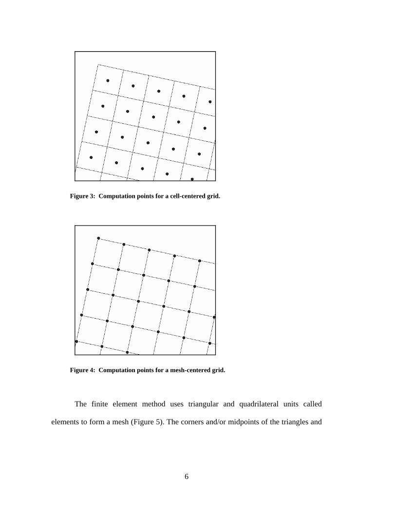
Figure 3: Computation points for a cell-centered grid.

Figure 4: Computation points for a mesh-centered grid.

The finite element method uses triangular and quadrilateral units called

elements to form a mesh (Figure 5). The corners and/or midpoints of the triangles and

6

quadrilaterals, called nodes, act as the computation points for finite element meshes

(Figure 6).

Figure 5: Elements forming a finite element mesh.

Figure 6: Computation points (nodes) for a finite element mesh.

In addition to discretizing the model domain into finite units, hydrologic and

hydraulic models require the specification of an elevation or depth value at each

7

computation point. This thesis uses the term z-value to refer collectively to elevation

and depth. Many models also require the specification of additional input parameters

at each computation point and/or over each finite unit.

2.1 Conceptual Modeling

Rather than creating each finite unit one at a time with their z-value and other

input parameters, a common modeling practice is to first create a conceptual model. A

conceptual model consists of a simplistic representation of the

situation being modeled. This includes the geometric attributes of the

situation (such as domain extents), the forces acting on the domain (such as

inflow or water level boundary conditions) and the physical characteristics

(such as roughness or friction). It does not include numerical details like

elements (3). A conceptual model consists of Geographic Information Systems (GIS)

objects such as feature points, lines and polygons. The location of the feature objects

and how they connect to each other delineate the model domain extents and form

boundaries where hydraulic parameters and/or geometric attributes change. Attributes

of the feature objects define the hydraulic parameters that will later be assigned to the

numerical finite units. Coverages, or layers, group feature objects with similar

attributes. One or many coverages make up a conceptual model (4, 5).

2.2 Automatic Meshing

Generating finite difference grids requires only the grid size, orientation and

cell sizes. Even complex grids with differing cell sizes in the i- and j-directions and

refinement around a specific location are trivial to create (Figure 7).

8

Figure 7: Finite difference grid with cell refinement around a point

On the other hand, creating unstructured grids (also referred to as finite

element meshes) involves non-trivial effort. Rather than defining each element by

hand, the conceptual model allows for the use of powerful automatic meshing

algorithms. Attributes tied to the feature polygons determine how elements fill in the

areas enclosed by the polygons. The spacing of the vertices along the features arcs

making up the polygon boundaries determines the density of the elements inside each

polygon. Figure 8 shows a simple polygon meshed using an algorithm known as

patching (6).

9

Figure 8: Feature polygon meshed using patching

2.3 Terrain Data

After generating a finite difference grid or finite element mesh, each

computation point needs a z-value. These z-values represent either elevation values

measured up from a datum or depth values measured down from a datum. For

hydrologic and hydraulic modeling purposes the terrain data contains bathymetry and

topography. Bathymetry describes surfaces covered by water such as river beds and

ocean floors. Topography describes land surfaces above water. With finite difference

grids, the modeler identifies the terrain data source when creating the grid. This allows

for automatic interpolation of z-values from the terrain data source to the cells of the

finite difference grid. With finite element meshes, each conceptual model feature

polygon contains an attribute linked to the terrain data source for automatic

interpolation to the nodes when creating the finite element mesh.

Two common ways of organizing and storing terrain data are Digital Elevation

Models (DEMs) and Triangulated Irregular Networks (TINs). A DEM is a raster, or

10

gridded, data structure containing a two-dimensional array of z-values at regularly

spaced horizontal intervals in both the x and y directions (Figure 9) (7).

Figure 9: A Digital Elevation Model (DEM).

A TIN is created from a set of input points with x,y-coordinate values as well

as z-values. These input points become triangle vertices, and lines connecting the

vertices form the triangle edges. The result is a continuous, piecewise linear surface of

non-overlapping triangles that border one another and vary in size and proportion

(Figure 10) (8). When integrating features into terrain data using feature stamping, the

terrain data must be in TIN format (1, 2). Conversion of terrain data in DEM format

into TIN format involves a minimal amount of effort.

11

Figure 10: A Triangulated Irregular Network (TIN).

2.4 Conceptual Model to Numerical Model

To generate a finite difference numerical model from a conceptual model, the

modeler first creates the finite difference grid. This also involves identifying the

terrain data source. The z-values for the cells are automatically interpolated from this

terrain data source when the grid is created. After creating the grid, the algorithm

maps the conceptual model to the numerical model. This assigns any hydraulic

parameters to the grid cells based on the zone of the conceptual model they lie in.

The modeler generates a finite element numerical model in a similar fashion.

For finite element meshes, converting the conceptual model to a numerical model

12

generates the mesh elements using the automatic meshing algorithms, interpolates the

z-values for each node from the terrain data source and assigns hydraulic parameters

to the nodes and elements based on their zone in the conceptual model.

Figure 11: Conceptual model of a river.

Figure 11 shows an example conceptual model of a river. Feature arcs form

feature polygons to identify the zones of the model having different hydraulic

characteristics. In this case, there are four major zones running the length of the river:

the left bank, the right bank, the main channel and a sandbar. Arcs going across the

river cut these major zones into additional polygons. Each polygon is tied to an

automatic meshing algorithm and a terrain data source. Figure 12 shows the finite

13

element mesh generated from this conceptual model. The mesh elements receive their

hydraulic properties based on their zone in the conceptual model.

Figure 12: Finite element numerical model of a river.

14

3 Previous Work

In 2001 Christensen implemented his feature stamping algorithms in SMS.

Figure 13 shows a schematic illustrating in general his feature stamping as

implemented in SMS.

Figure 13: Christensen’s implementation of feature stamping.

Conceptual

Model TIN

Feature Stamping

Conceptual Model w/ Stamped Feature

Create Numerical

Model

Numerical Model

15

This implementation requires as input, the conceptual model outlined with GIS

objects and terrain data stored as a TIN. To stamp a feature, a single arc on the same

coverage as the conceptual model represents the centerline of the feature. Attributes of

this centerline arc define the feature’s geometry with a single cross-section. The cross-

section included a horizontal center section having a non-zero width and could include

sloped side sections creating a roughly trapezoidal cross-section. Features with a

cross-section having only a horizontal center section with no side slopes were called

vertical-walled features. Features having a cross-section including side slopes were

called sloped features (Figure 14). After defining the feature’s cross-section, the

algorithm stamped the feature into the terrain. Stamping the feature creates additional

arcs in the conceptual model outlining the geometry of the feature and the intersection

between the feature and the terrain (Figure 15). The algorithm flagged these feature

arcs identifying them as arcs forming a stamped feature. In order to allow modification

of the stamped feature, the process then blocked the assignment of other attributes to

these arcs. Re-stamping a feature after modifying its centerline or cross-section deletes

the old stamped feature and creates a new one. The last step in Christensen’s

implementation of feature stamping involves converting the conceptual model that

contains the stamped feature to a numerical model (1, 2).

16

Figure 14: Vertical-walled versus sloped features.

Figure 15: Stamping a feature creates arcs outlining its resulting geometry.

Most hydrodynamic numerical models cannot have vertical cells/elements and

become unstable with steep cells/elements. If a modeler wants to integrate a stamped

feature having gentle slopes, he or she would use a sloped feature. Sloped features

allow water to flow across them. Figure 16 shows a simple flume with a groin stamped

17

as a sloped feature. Water flowing through the flume can flow around and over the

groin.

Figure 16: Sloped feature.

When stamping a feature that acts as a barrier to flow and does not allow water

to flow over it, a modeler would use a vertical-walled feature. Vertical-walled features

outline areas to mesh around or areas where the cells/elements are disabled. The

interface between enabled cells/elements and disabled ones acts as a vertical wall the

same way as the model’s open boundaries. Figure 17 shows a groin stamped as a

vertical-walled feature into a simple flume. In this case, the mesh goes around the

groin. Another option includes meshing the groin and disabling the elements forming

the groin. Water flows around this groin and can never flow over it.

18

Figure 17: Vertical-walled feature.

As explained in the previous paragraphs, Christensen’s original feature

stamping algorithms impose several geometric limitations on stamped features. A

feature used in these algorithms must have the same cross-section along its entire

length. The original feature stamping algorithms not only require a single cross-

section defining the entire feature, but also place geometric limitations on the cross-

section itself. The algorithms require trapezoidal cross-sections with a horizontal

center section having a non-zero width and sloped side sections having the same

simple slope (1, 2).

In addition to the geometric limitations, the original feature stamping

algorithms have several instabilities. First, if, during the process of stamping a feature,

the feature leaves the bounds of the terrain data, the feature stamping algorithms fail.

This failure also prevents stamped features with sloped sides from being created when

19

no terrain data exists at all. Another limitation appears when utilizing the resulting

conceptual model, and when attempting to modify the geometry of a feature and re-

stamp it. This is because the stamping process modifies the conceptual model and is

not identically invertible. When first stamping a feature, feature arcs are added to the

conceptual model to represent the geometry of the feature. Modifying the geometry of

the feature deletes these feature arcs and creates new ones (1, 2). The instability occurs

in keeping track of which feature arcs on the conceptual model to delete when the

geometry of the stamped feature changes.

20

4 Changes and Enhancements

As discussed in the previous chapter, Christensen’s feature stamping

algorithms have the following limitations and instabilities:

• Features must be prismatic

• Features must have symmetric, trapezoidal cross-sections

• The algorithms fail when sloped features leave the bounds of the terrain

• Re-stamping a feature is non-trivial and unstable

To eliminate these limitations and instabilities, Christensen’s feature stamping

algorithms have been rewritten using a more object oriented approach. Using such an

approach facilitates the future development of feature stamping. In addition to

rewriting the feature stamping algorithms, they have been expanded to include

algorithms for stamping radial features, such as borrow pits and mounds. The original

feature stamping algorithms base all features on a centerline (1, 2). Radial features, on

the other hand, base their geometries on a center point.

The remaining sections of this chapter discuss the changes made to

Christensen’s implementation of feature stamping and how these changes eliminate

the limitations and instabilities. Chapter 5 examines how the rewritten feature

21

stamping algorithms work with centerline-based features. Chapter 6 explains the

implementation of stamping radial features.

4.1 New Implementation

Figure 18 shows a schematic illustrating in general the new implementation of

feature stamping. The old implementation of feature stamping uses a conceptual

model approach to separate the definition of the stamped feature from the numerical

model. With this implementation, the definition of the stamped feature and the

stamped feature itself exist on the same coverage as the conceptual model (1, 2).

Figure 18: New implementation of feature stamping.

Feature

Stamping Coverage

TIN

Feature Stamping

Stamped Feature

Conceptual Model

Stamped Feature TIN

Create Numerical

Model

Conceptual Model

Numerical Model

22

However, having the stamped feature and the conceptual model on the same coverage

corrupts the conceptual model. Furthermore, the feature stamping algorithms fail in

keeping track of which arcs of the conceptual model pertain to stamped features and

which do not. This failure comes about when modifying the geometry of a stamped

feature and re-stamping it.

To eliminate this problem and maintain the integrity of the conceptual model,

the definition of the stamped feature lies on a separate coverage than the conceptual

model. Moreover, rather than stamping the feature directly to the conceptual model,

the new algorithms stamp the feature to still another coverage. This represents the

conceptual representation of the stamped feature, or simply, the stamped feature. The

feature stamping algorithms also stamp the z-values associated with the stamped

feature to its own TIN. This maintains the integrity of the input terrain data.

In summary, the input for the new implementation of feature stamping includes

the terrain data stored as a TIN and a coverage containing the definition of the

stamped feature. The results of stamping a feature include a coverage containing the

stamped feature and a TIN of the stamped feature’s z-values. The conceptual model

and input terrain data remain unchanged. The modeler creates a numerical model

integrating the stamped feature in one of several ways. This may included merging the

input terrain TIN and the stamped feature TIN to form a merged TIN, and/or merging

the conceptual model and the stamped feature to form a new conceptual model. The

tutorial in the Appendix discusses some methods for generating a numerical model

using the results of feature stamping and possible situations when each method might

be used.

23

Now, if the modeler decides to modify the alignment and/or geometry of the

stamped feature, he returns to the coverage containing the definition of the stamped

feature and makes his changes. Then, he re-stamps the feature. Re-stamping does not

stamp the feature to the same coverage and TIN as before, but to new ones. Therefore,

the modeler can either delete the coverage and TIN from previously stamping the

feature, or he can keep them for future use. In all instances, feature stamping maintains

the integrity of the conceptual model, the original terrain data, the definition of each

stamped feature and the coverages and TINs resulting from stamping the feature. It is

up to the modeler to combine these coverages and TINs to form the numerical model.

4.2 Specifying the Geometry

Rather than specifying a single cross-section for the entire length of the

feature, the new feature stamping algorithms allow the modeler to specify cross-

sections at each node and vertex along the centerline arc. This eliminates the

restriction of having prismatic features. Figure 19 shows a feature stamped by the old

feature stamping algorithms. This feature has the same cross-section along its entire

length. Figure 20 shows a feature stamped using the new feature stamping algorithms.

This feature has a different cross-section in its middle section.

24

Figure 19: Prismatic stamped feature.

Figure 20: Non-prismatic stamped feature.

To remove the restriction of having symmetric, trapezoidal cross-sections, the

new feature stamping algorithms treat each cross-section as two independent sides

divided by the centerline arc. A z-value and a horizontal distance from the centerline

25

arc identify the points making up the left and right sides of the cross-section. Each

proceeding cross-section point lies further away from the centerline arc than the

previous point. Figure 21 and Figure 22 show the left and right sides of an example

cross-section. The left side of the cross-section has a simple slope whereas the right

side has a compound slope. Table 1 shows the cross-section points making up both the

left and right sides of the cross-section. The modeler specifies each cross-section point

as a horizontal distance from the centerline and a z-value. Figure 23 shows a feature

stamped using this example cross-section

Left Side of Cross-Section

7.5

8

8.5

9

9.5

10

10.5

-1012345

Distance from Centerline (ft)

Ele

vatio

n (ft

)

Figure 21: Left side of cross-section.

26

Right Side of Cross-Section

7.5

8

8.5

9

9.5

10

10.5

-1 0 1 2 3 4 5 6 7


Elev

atio

n (ft

)

Figure 22: Right side of cross-section.

Table 1: Cross-section points for the left and right sides of the cross-section.

Left Side Right Side Distance

from Centerline

(ft)

Elevation (ft)

Distance from

Centerline (ft)

Elevation (ft)

0.0 10.0 0.0 10.0 2.0 10.0 2.0 10.0 3.0 9.0 3.0 9.0 4.0 8.0 5.0 9.0

6.0 8.0

27

Figure 23: Asymmetric, non-trapezoidal cross-section.

4.3 Maximum Distance

One of the instabilities in Christensen’s feature stamping algorithms occurs

when the feature leaves the extents of the terrain data. This occurs because the slope of

the feature continues to extend searching for an intersection with the terrain. Since no

possible intersection exists, an infinite loop occurs. Assigning a point at which to stop

extending the sides of the cross-section solves this problem. This stopping point is

referred to as the maximum distance. By default, the maximum distance is the

horizontal distance assigned to the last cross-section point. Increasing this maximum

distance causes the slope formed by the last two cross-section points to extend until it

intersects the terrain or reaches the maximum distance. By specifying a maximum

distance to extend each cross-section, feature stamping of sloped features does not fail

when the feature leaves the bounds of the terrain and even works when no terrain data

exists at all. Specifying a maximum distance is also useful when the modeler wants the

feature to intersect the terrain, but does not know where the intersection will occur.

Figure 24 shows a stamped feature whose right slope extends outside the domain of

28

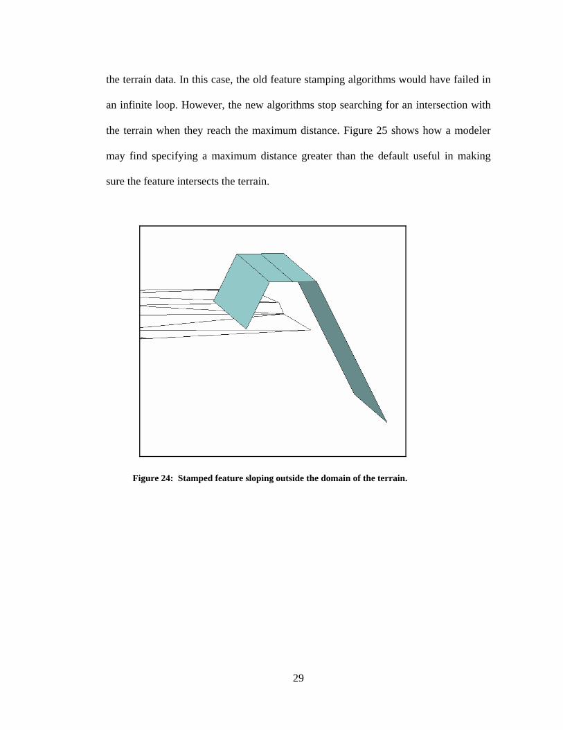
the terrain data. In this case, the old feature stamping algorithms would have failed in

an infinite loop. However, the new algorithms stop searching for an intersection with

the terrain when they reach the maximum distance. Figure 25 shows how a modeler

may find specifying a maximum distance greater than the default useful in making

sure the feature intersects the terrain.

Figure 24: Stamped feature sloping outside the domain of the terrain.

29

Figure 25: Increasing the maximum distance extends the cross-section.

30

5 Centerline-Based Features

Christensen’s original feature stamping algorithms base all features on a

centerline (1, 2). This section describes how the new feature stamping algorithms

stamp centerline-based features. The new algorithms maintain all the functionality of

the original algorithms, but allow for the stamping of features having more complex

geometries.

The feature stamping algorithms stamp two general types of features: fill

features and cut features. Fill features, such as embankments, levees and berms, build

upon the existing terrain. In Christensen’s thesis, he generally refers to these types of

features as embankments (1, 2). For fill features, the feature stamping algorithms only

stamp the parts of the feature situated above the terrain. The intersection between the

feature and the terrain becomes the extents of the feature. Cut features, such as

channels and pits, remove existing terrain. Christensen’s thesis generally refers to

these types of features as channels (1, 2). For cut features, the feature stamping

algorithms only stamp the parts of the feature situated below the terrain. Figure 26 and

Figure 27 show a fill feature and a cut feature, respectively.

31

Figure 26: Fill feature.

Figure 27: Cut feature.


A modeler defines the geometry of centerline-based features in four steps.

First, he defines an arc along the centerline of the feature. Second, he identifies the

32

feature as either a fill or cut feature. Third, he defines a cross-section at each node and

vertex of the centerline arc. Fourth, he selects an end cap for both ends of the feature.

5.1.1 Defining the Centerline Arc

The centerline arc serves three purposes: to position the feature, to determine

the number of cross-sections required to describe the geometry of the feature and to

provide a starting point for defining each cross-section. The position of the centerline

arc determines the feature’s general shape, size and location with respect to the terrain.

In most cases, as the name implies, the centerline arc exists along the centerline of the

feature. However, it may exist along any line of reference on the feature.

Each node and vertex along the centerline arc requires a cross-section.

Understanding this principle helps in strategically placing the vertices of the centerline

arc. The feature’s shape determines the minimum required number of vertices. The

feature stamping algorithms require a vertex anytime the feature changes direction and

whenever the cross-section of the feature changes. Therefore, a straight prismatic

feature theoretically requires only two cross-sections, one at each end. However, detail

in how the feature intersects the terrain may be lost between these two cross-sections.

Therefore, the modeler should place additional vertices periodically along straight

portions of the centerline arc. Shallow slopes in the terrain require fewer vertices

whereas steep slopes require more densely spaced vertices. Figure 28 shows a

centerline-based feature defined with two cross-sections. Figure 29 shows the same

feature defined with ten cross-sections. The feature with ten cross-sections more

accurately intersects the terrain.

33

Figure 28: Centerline-based feature with two cross-sections.

Figure 29: Centerline-based feature with ten cross-sections.

The centerline nodes and vertices act as the starting point for defining cross-

sections. Before defining cross-sections, the modeler assigns each node and vertex a z-

value to form the profile of the feature. He may specify a flat or varying profile.

Figure 30 shows a feature with a varying profile along the length of its centerline.

Once the modeler has defined the profile of the centerline arc, he defines the cross-

sections at each node and vertex.

34

Figure 30: Feature with varying profile along the centerline.

5.1.2 Defining Cross-Sections

The centerline nodes or vertices divide the cross-sections into two sides. From

the centerline point, the modeler defines the left and right sides of each cross-section

in three steps. First, he adds cross-section points to define the shape of the cross-

section. Second, he identifies one cross-section points on each side as a shoulder point.

Third, he specifies the maximum distance to extend each side of the cross-section.

The two sides of a cross-section start off with one shared point, the node or

vertex of the centerline arc. The modeler has already assigned this point a z-value.

Adding subsequent points to a cross-section side requires specifying a positive

horizontal distance away from the centerline point and a z-value. The z-values can

vary up or down from one cross-section point to the next, but the horizontal distances

should continually increase. This prevents cross-sections with vertical faces and

35

overhangs. Feature stamping prohibits such cross-sections because most two-

dimensional hydrodynamic models prohibit vertical or overhanging elements. Figure

31 and Figure 32 plot the left and right sides of a sample cross-section. Table 2

provides their cross-section points.

Left Side of Cross-Section

7.5

8

8.5

9

9.5

10

10.5

-1012345


Ele

vatio

n (ft

)

Figure 31: Left side of cross-section.

Right Side of Cross-Section

7.5

8

8.5

9

9.5

10

10.5

-1 0 1 2 3 4 5 6 7


Elev

atio

n (ft

)

Figure 32: Right side of cross-section.

36

Table 2: Cross-section points for the left and right sides of the cross-section.

Left Side Right Side Distance

from Centerline

(ft)

Elevation (ft)

Distance from

Centerline (ft)

Elevation (ft)

0.0 10.0 0.0 10.0 2.0 10.0 2.0 10.0 3.0 9.0 3.0 9.0 4.0 8.0 5.0 9.0

6.0 8.0

Since each cross-section can have a different number of points, the stamped

feature cannot include arcs connecting all the points in one cross-section to all the

points in adjacent cross-sections. Therefore, three types of cross-sections points act as

connection points. First, the points along the centerline connect to each other. Second,

the left and right boundary points connect. Third, one additional arc connects a cross-

section point on the left side of a cross-section to a cross-section point on the left side

of adjacent cross-sections. Similarly, an additional arc connects one point on the right

sides (Figure 33). These additional connection points are called shoulder points.

Shoulder points from one cross-section to the next do not require the same horizontal

distance or z-value. The modeler specifies the shoulder points for the left and right

sides of a cross-section independent of each other. By default, feature stamping sets

the centerline points as the shoulder points. Figure 33 labels the centerline, shoulders

and boundaries of a simple stamped feature.

37

Figure 33: Centerline, shoulders, and boundaries of a stamped feature.

Assigning a maximum distance to extend the left and right sides of each cross-

section keeps the feature stamping algorithms from going into an infinite loop when

searching for an intersection with the terrain. No intersection with the terrain exists

when the feature slopes outside the bounds of the terrain, when the feature slopes in

the opposite direction of the terrain or when no terrain data exists at all. The modeler

specifies the maximum distance as a horizontal distance from the centerline point. He

specifies the maximum distance for the left and right sides of a cross-section

38

independent of each other. Likewise, the maximum distances from one cross-section

to the next can vary. By default, the feature stamping algorithms use the horizontal

distance of the last point of the left and right sides of a cross-section side as its

maximum distances. A maximum distance greater than the default causes the slope

formed by the last two cross-section points to extend until it intersects the terrain or

reaches the maximum distance.

5.1.3 Selecting End Caps

There are three types of end caps: sloped abutments, wing walls and

guidebanks. The feature stamping algorithms use sloped abutments with no slope as

the default. Like all other cross-sections, the feature stamping algorithms interpret the

two end cross-sections as perpendicular to the centerline. However, the modeler can

specify an angle at which to rotate the end cross-sections (Figure 34). Each end can

have a different cross-section angle.

The modeler specifies sloped abutments similarly to the cross-section sides

along the centerline. The end point of the centerline acts as the starting point for the

sloped abutment cross-section. The modeler specifies subsequent points as a

horizontal distance from this point and a z-value. The z-value can vary up or down

from one cross-section point to the next, but the horizontal distance should continually

increase. As with cross-sections, the modeler can specify a maximum distance to

extend the sloped abutment cross-section. Figure 35 shows a stamped feature with a

sloped abutment end cap.

39

Figure 34: Rotated end cross-section.

Figure 35: Sloped abutment end cap.

The modeler should only use wing wall end caps when stamping vertical-

walled features. A single parameter, the wing wall angle, defines a wing wall end cap.

40

Figure 36 shows the wing wall angle. The feature stamping algorithms create wing

walls by rotating the parts of the end cross-sections past the shoulder points by the

wing wall angle. This rotation occurs after the end cross-sections have been rotated by

the cross-section angle. Figure 37 shows a vertical-walled stamped feature with a wing

wall end cap.

Figure 36: The wing wall angle.

Quarter ellipse extensions to centerline-based features form guidebank end

caps. These extensions direct the flow of water around a structure. When using

guidebanks, the feature stamping algorithms use the end cross-section as the cross-

section for the entire guidebank. Therefore, when using guidebanks, the modeler only

specifies the side of the feature the guidebank lies on, the width of the guidebank, the

two radii of the ellipse and the number of points to distribute along the guidebank.

Similar to the centerline arc, the more points along the guidebank, the more detailed

the intersection of the guidebank with the terrain.

41

Figure 37: Wing wall end cap.

5.2 Stamping the Feature

The feature stamping algorithms stamp centerline-based features in five steps.

First, they convert the centerline, cross-sections and end caps definition into a three-

dimensional representation of the feature. Second, they intersect the centerline with

the terrain. Third, they intersect the cross-sections with the terrain. Fourth, they

remove cross-sections with a centerline point on the wrong side of the terrain. Fifth,

they stamp the end caps.

5.2.1 Converting to Three-Dimensions

Converting the centerline, cross-sections and end cap definitions to a three-

dimensional definition begins with the centerline because the modeler has already

42

defined it in three-dimensions. Next, the feature stamping algorithms convert the

cross-sections and end caps to three-dimensions.

The first and last cross-sections extend perpendicular to the centerline (Figure

38). Intermediate cross-sections extend so that they bisect the two centerline segments

connected to their centerline points (Figure 39). Knowing the location of the centerline

points and at what angles the cross-sections extend, the feature stamping algorithms

convert the horizontal distances and z-values of the cross-section points into 3D

locations. When converting the last cross-section points on both cross-section sides,

the feature stamping algorithms use the maximum distance rather than the point’s

horizontal distance. The algorithms adjust the z-value of the point to match the

maximum distance.

Figure 38: End cross-sections extend perpendicular to the centerline.

43

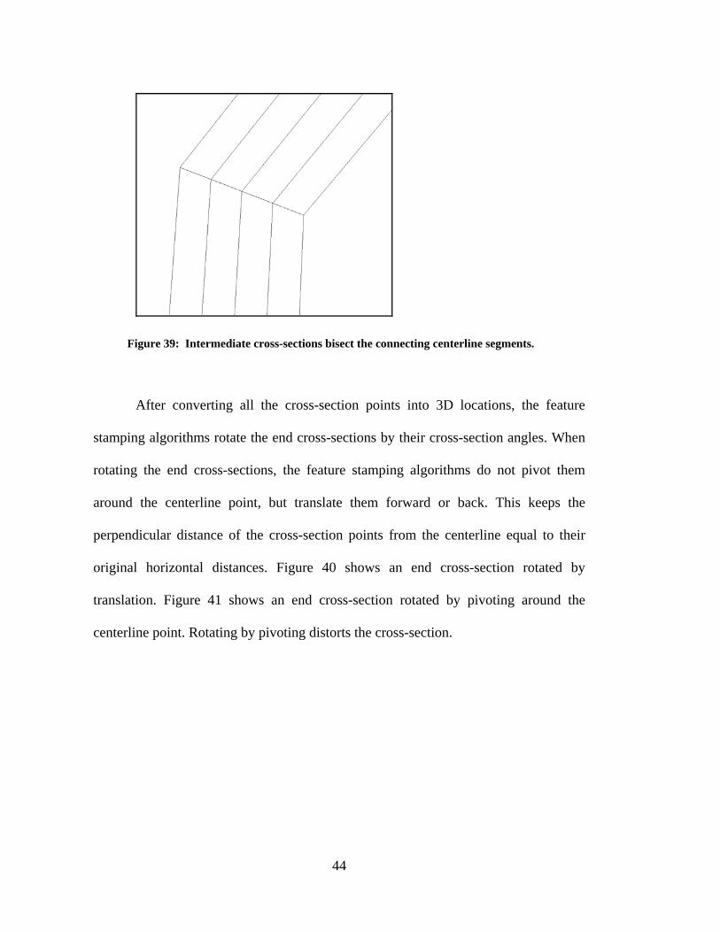
Figure 39: Intermediate cross-sections bisect the connecting centerline segments.

After converting all the cross-section points into 3D locations, the feature

stamping algorithms rotate the end cross-sections by their cross-section angles. When

rotating the end cross-sections, the feature stamping algorithms do not pivot them

around the centerline point, but translate them forward or back. This keeps the

perpendicular distance of the cross-section points from the centerline equal to their

original horizontal distances. Figure 40 shows an end cross-section rotated by

translation. Figure 41 shows an end cross-section rotated by pivoting around the

centerline point. Rotating by pivoting distorts the cross-section.

44

Figure 40: Translating the cross-section points forward and back.

Figure 41: Pivoting the cross-section points around the centerline point.

When converting sloped abutments to a 3D representation, the feature

stamping algorithms rotate the parts of the end cross-sections past the shoulder points

to run perpendicular to the centerline. Again, translating these points maintains the

perpendicular distance from the centerline. Figure 42 shows a stamped feature having

a sloped abutment end cap. Since the modeler has specified a cross-section angle, the

45

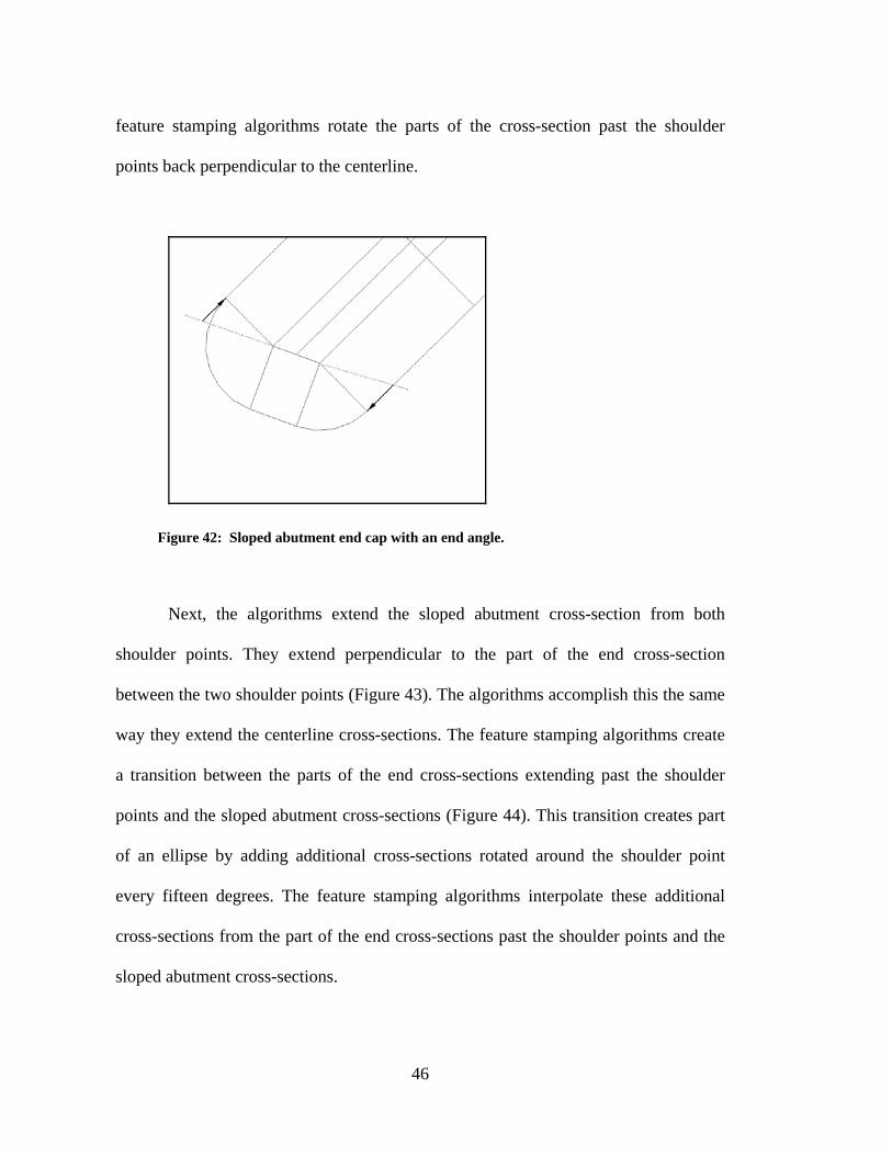
feature stamping algorithms rotate the parts of the cross-section past the shoulder

points back perpendicular to the centerline.

Figure 42: Sloped abutment end cap with an end angle.

Next, the algorithms extend the sloped abutment cross-section from both

shoulder points. They extend perpendicular to the part of the end cross-section

between the two shoulder points (Figure 43). The algorithms accomplish this the same

way they extend the centerline cross-sections. The feature stamping algorithms create

a transition between the parts of the end cross-sections extending past the shoulder

points and the sloped abutment cross-sections (Figure 44). This transition creates part

of an ellipse by adding additional cross-sections rotated around the shoulder point

every fifteen degrees. The feature stamping algorithms interpolate these additional

cross-sections from the part of the end cross-sections past the shoulder points and the

sloped abutment cross-sections.

46

Figure 43: Sloped abutment cross-sections extend from the shoulder points.

Figure 44: The elliptical transition for sloped abutments.

The feature stamping algorithms convert wing walls to 3D by rotating the parts

of the end cross-sections past the shoulder points by the wing wall angle (Figure 45).

Again, translating the end cross-section points maintains their perpendicular horizontal

distance.

47

Figure 45: Rotating back the cross-section to form wing wall end caps.

The feature stamping algorithms treat guidebanks as a separate stamped

feature. However, with guidebanks, the modeler does not directly define the

guidebank centerline points. Therefore, when converting guidebanks to 3D, the feature

stamping algorithms first create the centerline points based on the two radii and the

desired number of points. Once these guidebank centerline points have been located in

3D, the feature stamping algorithms convert the rest of the guidebank just like a

centerline-based feature with a sloped end cap.

5.2.2 Intersecting the Centerline

Tracing the centerline through the TIN triangles of the terrain determines

where the centerline and terrain intersect. The feature stamping algorithms start this

process by locating which triangle the first centerline point lies in. The feature

stamping algorithms check each triangle the centerline passes through from the first

point to the second point to see if the first centerline segment intersects them. Rather

than searching the entire TIN for each subsequent triangle, the feature stamping

48

algorithms use the 2D equation of the line segment to trace through the TIN triangles

in a more efficient manner. If the centerline segment intersects the terrain, the feature

stamping algorithms add a point to the centerline at the intersection. The feature

stamping algorithms interpolate the cross-section assigned to the intersection point

from the cross-sections on either side. Checking the remaining centerline segments in

a similar manner locates all intersections with the terrain.

5.2.3 Intersecting the Cross-sections

The feature stamping algorithms intersect the terrain with the cross-sections in

a similar manner to how they intersect the centerline. First, they intersect the lefts

sides of each cross-section and then the right sides. The algorithms locate the triangle

containing the centerline point. Checking all the triangles the cross-sections pass

through from point to point determines if the cross-section intersects the terrain. If the

feature stamping algorithms find an intersection, they add a point to the cross-section

and remove the remaining cross-section points. If the feature stamping algorithms do

not find an intersection, they conclude tracing through the triangles when they reach

the last cross-section point.

5.2.4 Removing Cross-sections

After finding where the centerline and cross-sections intersect the terrain, the

feature stamping algorithms remove cross-sections having centerline points on the

wrong side of the terrain. For fill features, the feature stamping algorithms remove

cross-sections below the terrain. For cut features, the feature stamping algorithms

remove cross-sections above the terrain. Removing cross-sections after find where the

49

centerline and cross-sections intersect the terrain allows the centerline to pass through

the terrain onto the wrong side and later return to the correct side.

5.2.5 Stamping the End Caps

Each end cap is composed of a series of cross-sections. Therefore, the feature

stamping algorithms find where end caps intersect the terrain the same way they

intersect the cross-sections along the centerline. If the feature stamping algorithms

remove the end cross-sections because they lie on the wrong side of the terrain, then

they do not stamp the end caps. In addition to cross-sections, guidebanks also include

a centerline. The feature stamping algorithms find where this centerline intersects the

terrain the same way they find where the main centerline intersects the terrain.

50

6 Radial Features

In addition to eliminating the instabilities and limitations of Christensen’s

feature stamping algorithms which base all features on a centerline, the new feature

stamping algorithms contain additional options for stamping radial features based on a

center point. The following sections explain how the modeler defines radial features

and how the feature stamping algorithms stamp them.


A modeler defines the geometry of radial features in three steps. First, he

defines the location of the point at the center of the feature. Second, he identifies the

feature as either a fill or cut feature. Third, he defines the feature’s cross-section.

The center point serves three purposes: to position the feature, to operate as

the first cross-section point and to act as the pivot for rotating the cross-section about

when forming the stamped feature. By positioning the center point and assigning it a

z-value, the modeler locates the feature with respect to the terrain. For fill features, the

modeler must locate the center point above the terrain. Otherwise, the feature

stamping algorithms will not stamp the feature. For cut features, the modeler must

locate the center point below the terrain (Figure 46).

51

Figure 46: Locating the center point for fill and cut features.

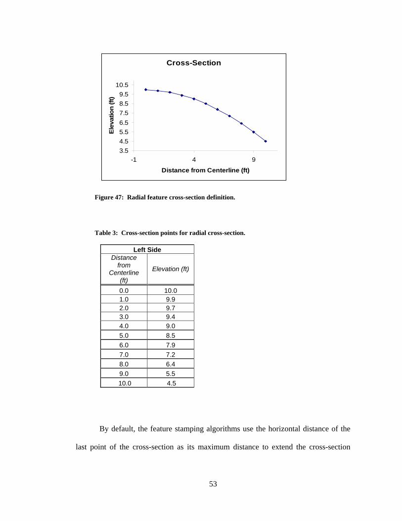
A single cross-section defines the shape of a radial feature. The cross-section

begins with the center point which already has a z-value. The modeler adds

subsequent cross-section points by specifying a positive horizontal distance away from

the center point and a z-value. Like with the cross-sections of centerline-based

features, the z-values can vary up or down from one cross-section point to the next,

but the horizontal distances must continually increase. Figure 47 plots the points

defining an example radial feature cross-section. Table 3 shows the values of these

points.

52

Cross-Section

3.54.55.56.57.58.59.5

10.5

-1 4 9


Elev

atio

n (ft

)

Figure 47: Radial feature cross-section definition.

Table 3: Cross-section points for radial cross-section.

Left Side Distance

from Centerline

(ft)

Elevation (ft)

0.0 10.0 1.0 9.9 2.0 9.7 3.0 9.4 4.0 9.0 5.0 8.5 6.0 7.9 7.0 7.2 8.0 6.4 9.0 5.5

10.0 4.5

By default, the feature stamping algorithms use the horizontal distance of the

last point of the cross-section as its maximum distance to extend the cross-section

53

away from the center point. However, the modeler can increase this maximum

distance. A maximum distance greater than the default causes the slope formed by the

last two cross-section points to extend until it intersects the terrain or reaches the

maximum distance. Specifying a maximum distance greater than the default is useful

when the modeler wants the feature to intersect the terrain, but does not know where

the intersection will occur. Figure 48 shows a radial feature cross-section that does not

intersect the terrain when extending only to the last cross-section point. However,

increasing the maximum distance causes the cross-section to intersect the terrain.

Figure 48: Increasing the maximum distance extends the cross-section.

6.2 Stamping Radial Features

The feature stamping algorithms stamp radial features in two steps. First, they

convert the center point and cross-section to a three-dimensional representation of the

54

feature. Second, they intersect the cross-sections of the three-dimensional

representation with the terrain.

Because the modeler has already defined the center point in 3D space,

converting the center point and cross-section to a three-dimensional representation

begins with the center point. Next, the feature stamping algorithms convert the cross-

section to three-dimensions by extending it away from the center point every fifteen

degrees for a total of 24 cross-sections. Knowing the location of the center point and

the angles the cross-sections extend, the feature stamping algorithms convert the

horizontal distances of the cross-section points into locations in 3D space. The z-

values of the cross-section points require no conversion. When converting the last

cross-section point, the feature stamping algorithms use the maximum distance rather

than the point’s horizontal distance. The feature stamping algorithms adjust the z-

value of this point to match the maximum distance.

The feature stamping algorithms intersect each of the 24 cross-sections

extending away from the center point by first finding the TIN triangle containing the

center point. For each cross-section the feature stamping algorithms proceed from the

center point down the cross-section checking the triangles crossed to see if the cross-

section intersects the terrain. If the algorithms find an intersection, they add the

intersection point to the cross-section and remove any remaining cross-section points.

The feature stamping algorithms finish tracing a cross-section through the TIN

triangles when they reach the last cross-section point. Figure 49 shows an example of

a radial feature.

55

Figure 49: Radial feature.

56

7 Conclusion

As more civil engineers begin to use numerical models to analyze hydrologic

and hydraulic processes, the ability to quickly integrate man-made features into

surveyed terrain data becomes increasingly important. Christensen developed such a

tool for integrating geometric features into terrain data. He dubbed this process feature

stamping. His feature stamping algorithms decrease the time and effort required to

integrate geometric features into existing terrain data. However, these algorithms

possess several instabilities and limitations. First, Christensen’s feature stamping

algorithms enter an infinite loop and fail when stamping features that leave the bounds

of or slope away from the terrain data. This failure also prevents stamped features with

sloped sides from being created when no terrain data exists at all. Second,

Christensen’s feature stamping algorithms fail when using a stamped feature,

modifying its geometry and re-stamping it. Finally, Christensen’s feature stamping

algorithms only work with centerline-based features having a constant trapezoidal

cross-section.

7.1 Changes and Enhancements

This thesis described changes and enhancements made to the feature stamping

algorithms to eliminate the instabilities and geometric limitations. With the new

57

feature stamping algorithms, numerical modelers can now stamp more complex

geometric features having compound slopes, asymmetric cross-sections and varying

cross-sections along their length. Furthermore, the new feature stamping algorithms

include additional algorithms for stamping radial features such as mounds and pits.

Not only do the new feature stamping algorithms eliminate the geometric limitations,

but they also eliminate the instabilities. The new feature stamping algorithms do not

fail when stamping features that leave the bounds of or slope away from the terrain

data. Moreover, the new algorithms can stamp feature even when no terrain data exists

at all. Finally, the new feature stamping algorithms stabilize the process of stamping a

feature, modifying its geometry and re-stamping it, preserving the integrity of the

conceptual model and input terrain data.

7.2 Future Considerations

Although improved greatly, several future considerations for feature stamping

exist. These include:

• Additional types of end caps

• Features based on a center polygon

• Clean-up algorithms

The following sections briefly describe each future consideration.

7.2.1 Additional Types of End Caps

The research for this thesis did not include any additional types of end caps.

However, the fact that the new feature stamping algorithms are written in a more

object-oriented simplifies the process of adding of other types of end caps. Adding an

58

option of stamping another type of end cap involves deciding what parameters define

the geometry of the end cap and adding the algorithms convert the end cap definition

into a 3D representation. No changes would have to be made to the existing

algorithms.

7.2.2 Features Based on a Center Polygon

Christensen’s feature stamping algorithms based all features on a centerline.

The research for this thesis expanded the feature stamping algorithms to include radial

features, or features based on a center point. Future development of feature stamping

may include algorithms for stamping features based on a center polygon. The

definition of such features would include a center polygon and cross-sections to be

extended from each polygon vertex at a bisecting angle. The feature stamping

algorithms would stamp features based on a polygon in a similar manner to how they

stamp centerline-based features. First, the algorithms would intersect the center

polygon with the terrain data and remove those parts of the polygon on the wrong side

of the terrain. Then, the feature stamping algorithms would intersect each cross-

section with the terrain. Figure 50 shows how a stamped feature based on a center

polygon might look.

59

Figure 50: Feature based on a center polygon.

7.2.3 Clean-Up Algorithms

When stamping a feature that bends sharply, the cross-sections can overlap

each other as shown in Figure 51. The new feature stamping algorithms remain stable

when stamping such features; however, they do not do any clean-up to correct the

problems resulting from the overlapping cross-sections. The modeler can fix these

problems by hand, but this can be difficult. Adding algorithms to clean-up the

problems created by overlapping cross-sections would greatly benefit the feature

stamping process.

The main clean-up strategy would be to check for overlapping cross-sections

after intersecting a cross-section with the terrain. After intersecting a cross-section

with the terrain, the feature stamping algorithms would see if the cross-section

overlaps any cross-sections that have previously been intersected with the terrain.

Overlaps are not necessarily 3D intersections, but intersections in 2D. If an overlap

60

Figure 51: Feature with a sharp bend resulting in overlapping cross-sections.

occurs, the algorithms add the point of overlap to both cross-sections and remove the

remaining points of both cross-sections. The z-value for the point of overlap would be

interpolated from the cross-section points on either side of the point. After the feature

stamping algorithms intersect the centerline and cross-sections, they form the

boundary of the feature. When forming the boundary, checks are done to see if the

lines forming the boundary overlap any cross-sections. If the boundary overlaps a

cross-section, the point of overlap is added to the cross-section and the remaining

cross-section points are removed. Figure 52 shows the centerline-based features from

Figure 51 after employing the previously explained clean-up strategy. This clean-up

61

strategy would work when stamping end caps as well since the feature stamping

algorithms form end caps with cross-sections and boundary lines.

Figure 52: Feature with overlapping cross-sections after clean- up.

62

Appendix: Feature Stamping Tutorial for SMS 9.0

63

Introduction

In this lesson you will learn how to use conceptual modeling techniques to

create numerical models that incorporate flow control structures into existing

bathymetry. The flow control structures you will be creating are abutments for a

proposed bridge over Double Pipe Creek near Detour, Maryland. To do this you will

be using feature stamping. The input files needed to complete this tutorial are found on

the CD included in the back. A demo version of SMS 9.0 can be requested from EMS-I

at www.ems-i.com.

Opening a Background Image

To provide a base map and to help you place the centerlines for the abutments

of the proposed bridge you will open an aerial photograph of Double Pipe Creek near

Detour, Maryland. To open the image:

1. Select File | Open.

2. Select DoublePipeCreekPhoto.jpg in the tutorial\Feature Stamping directory

and click the Open button.

3. Depending on your preference settings, SMS may ask if image pyramids are

desired. It is advised that you select the toggle to not ask this question again

and click Yes.

SMS displays the aerial photograph (Figure 53).

65

Figure 53: Aerial photograph of Double Pipe Creek near Detour, Maryland.

Specifying the Coordinate System

The image has now been read into SMS, but SMS has not been told what

coordinate system the data is referenced to. The coordinate system is dependent on the

data source. To specify the coordinate system:

1. Select Edit | Current Coordinates.

2. Leave the Horizontal System as “Local”, but change the Horizontal and

Vertical Units to “U.S. Survey Feet.”

66

Importing Bathymetric Data

For this lesson you will use bathymetry from a survey of the area around

Double Pipe Creek near Detour, Maryland before construction of the elevated road

and bridge. To bring the survey data into SMS:

1. Select File | Open.

2. Select detour.xyz and click the Open button.

3. The File Import Wizard dialog will appear. Click Next to proceed to step 2 of

the File Import Wizard.

4. Click Finish to close the File Import Wizard and import the survey data.

Figure 54: Bathymetry for Double Pipe Creek and its floodplain.

67

This survey file contains elevation data for Double Pipe Creek and its

floodplain which includes the town of Detour, Maryland. The survey data has already

been adjusted to the same local coordinate system as the image. Transparent contours

of the survey points displayed over the background image are shown in Figure 54.

Creating the Model Domain

Before creating a numerical model, a conceptual model will be created to

define the extents of the model domain. By using a conceptual model, you can take

advantage of automatic meshing algorithms. The two sides of the model domain

running along the length of Double Pipe Creek will be formed by extracting the 330

foot contour from the survey data. The ends of these two boundaries will then be

connected to create the upstream and downstream boundaries of the model domain. To

define the model domain:

1. Right-click on the Map Data item in the Project Explorer and select the New

Coverage menu item. A new coverage will be added to the Project Explorer

named new coverage.

2. Click on the new coverage coverage in the Project Explorer to activate it.

3. Right-click on the new coverage coverage in the Project Explorer and select

the Rename menu item. Rename the coverage “Double Pipe Bridge.”

4. Right-click on the Double Pipe Bridge coverage in the Project Explorer and

select the Type | TABS menu item to specify that this coverage will be used to

develop a conceptual model for the TABS package.

68

5. Right-click on the detour scatter set in the Project Explorer and select the

Convert | Scatter Contours -> Map menu item.

6. Enter an Elevation of 330 feet and a Spacing of 100 feet in the Create Contour

Arcs dialog.

7. Click OK to close the Create Contour Arcs dialog and generate arcs along the

330 foot contour. The resulting arcs run along the length of Double Pipe Creek.

A single looped arc is created on the extreme east side of the scatter set. Delete

this arc.

Figure 55: Model domain of Double Pipe Creek.

69

8. With the Create Feature Arc tool create the upstream and downstream

boundaries of the model domain as shown in Figure 55. Delete any dangling

arcs that result when creating these two boundaries.

The model domain extents are now defined in the Double Pipe Bridge

coverage. It is important to note than when creating a finite element mesh from a

conceptual model, the bathymetry is interpolated from the scatter set. Therefore, the

conceptual model should be within the bounds of the scatter set to avoid difficulties

that arise when extrapolating data.

Creating the Abutments

As mentioned above the abutments of the proposed roadway will be created

using feature stamping. This lesson presents stamping the abutments for the proposed

bridge over Double Pipe Creek in five steps: setting up a Stamping coverage,

positioning the abutments, specifying the geometry of the abutments, stamping the

abutments into the existing bathymetry and incorporating the stamped features into the

numerical model.

Setting Up a Stamping Coverage

SMS includes a coverage type, called a Stamping coverage, for positioning and

defining the geometry of features to be forced into existing bathymetry using feature

stamping. To setup the Stamping coverage for this lesson:

1. Create a new coverage, name it “Feature Stamp”, set its Type to Stamping and

activate it.

70

2. Right-click on the Feature Stamp coverage in the Project Explorer and

select the Properties menu item to bring up the Stamping Coverage Attributes

dialog.

3. In the Stamping Coverage Attributes dialog select the elevation (Z) item in

the tree control and leave the Bathymetry Type as “Elevation.” This sets the

elevation (Z) dataset of the detour scatter set as the bathymetry the stamped

features will be forced into. Furthermore, by leaving the Bathymetry Type as

“Elevation,” you tell SMS that the selected dataset contains elevation values

rather than depth values.

4. Click OK to close the Stamping Coverage Attributes dialog.

Positioning the Abutments

You will position the abutments by creating feature arcs along their

centerlines. The accuracy in how the abutments intersect the existing bathymetry

depends on how many vertices are distributed along the centerline arcs. For this lesson

you will distribute the vertices so they are closer together where the slope of the

bathymetry changes rapidly near the banks of the creek and further apart where the

slope is nearly flat in the floodplain. To create the centerline arcs for the abutments:

1. Using the Create Feature Arc tool create arcs representing the centerlines of

the two abutments as shown in Figure 56. You can use the roadway in the

aerial photograph to help you position the centerline arcs and line them up with

each other. Create the arcs starting outside the model domain in the floodplain

and proceeding toward the Double Pipe Creek. Terminate the arcs at the edge

71

of the creek. The length of the bridge will be roughly the distance between the

two nodes. You may have to adjust your display options or zoom in to

better see the model domain on the Double Pipe Bridge coverage.

2. With the Select Feature Arc tool, select the centerline arc for the west

abutment and select Feature Objects | Redistribute Vertices. This brings up the

Redistribute Vertices dialog.

3. In the Redistribute Vertices dialog set Specify to “Number of Segments,” the

Num Seg to 6 and the Bias to 0.1. Click OK to close the Redistribute Vertices

dialog.

4. Redistribute the vertices along the centerline for the east abutment in a similar

manner using 10 segments.

Figure 56: Abutment centerlines for the proposed bridge over Double Pipe Creek.

72

Specifying the Geometry of the Abutments

Now that the abutments have been positioned with centerline arcs you can

specify their geometry. To specify the geometry of the abutments:

1. With the Select Feature Arc tool double-click on the west abutment. This

brings up the Stamping Arc Attributes dialog.

2. In the Stamping Arcs Attributes dialog specify the Feature Name as “West

Abutment.” Leave the Stamping Type as “Fill Feature” since this abutment will

be increasing the elevation of the existing bathymetry.

3. Click the Constant -> Elevation button in the Centerline (CL) Profile area to

bring up the Constant -> Elevation dialog. Enter a constant elevation of 332

feet and click OK to close the dialog. This sets the elevation at each of the

points along the centerline arc to 332 feet. The elevations for the points along

the centerline can be set one at a time in the Centerline (CL) Profile

Spreadsheet or all at once using the macros found below this spreadsheet.

4. Note that the first point along the centerline is marked with an arrow . This

arrow identifies the current point. The Cross-sections (CS) area of the

attributes dialog displays the cross-section for the current point for viewing and

editing. When the current point is changed by clicking on it in the Centerline

(CL) Profile Spreadsheet, the Cross-sections (CS) area updates to display the

cross-section of the new current point. You will now specify the cross-sections

at each point along the centerline.

5. In the Cross-sections (CS) area click the Specify Top Width and Single Side

Slopes macro button to bring up the Top Width and Side Slopes dialog. Enter a

73

Top Width of 25 feet and Left and Right Slopes of -1. Click OK to close the

dialog. A simple cross-section has now been specified. To ensure these cross-

sections intersect the bathymetry when being stamped, specify a Maximum

Distance from CL of 35 feet for both the left and right sides of the cross-

section.

6. Copy this cross-section to the remaining centerline points by clicking the

Current CS -> All CS macro button. Click Yes when prompted to adjust the

cross-sections based on the centerline elevation.

7. To specify a slope on the end of the abutment click the Last End Cap button to

bring up the Last End Cap dialog. Leave the Type of end cap as “Sloped

Abutment” and the Angle as 0.0°. In the last line of the Slope Spreadsheet enter

a Distance from CS of 1 foot and an Elevation of 331 feet. To ensure the

sloped abutment intersects the bathymetry, specify a Maximum Distance from

CS of 25 feet.

8. Click OK twice to exit the Last End Cap and Stamping Arc Attributes dialogs.

9. Repeat steps 1 through 8 for the east abutment except set the Feature Name to

“East Abutment.”

The geometry for both the abutments has now been specified. For this lesson

you are creating fairly simple features to force into the existing bathymetry. The

feature stamping interface inside SMS has been designed to make creating these

simple features quick but at the same time allowing for the creation of more complex

features. You are now ready to stamp the abutments and add them to the conceptual

model.

74

Stamping the Abutments

To maintain the integrity of the conceptual model and the existing bathymetry,

feature stamping creates a new coverage and a new scatter set for each stamped

feature. If the conceptual model or the existing bathymetry becomes corrupted, it

makes it difficult to test several scenarios for the placement and geometric design of

features being stamped. To stamp the abutments into the existing bathymetry:

1. Select Feature Objects | Stamp Features to bring up the Stamp Features

dialog.

2. In the Stamp Features dialog make sure the Coverage Type is set to “TABS”

and click Stamp.

You will notice a coverage and scatter set are added to the Project Explorer for

the west abutment and also for the east abutment.

Incorporating the Abutments into a Numerical Model

There are three methods for incorporating stamped features into a numerical

model. With Method 1 only the scatter set of the stamped feature is used. With

Method 2 only the coverage of the stamped feature is used. Finally, with Method 3

both the scatter set and the coverage of the stamped feature are used. The following

paragraphs describe the how to use each method.

Method 1: To use just the scatter set of the stamped feature as part of the

conceptual model, it must be merged with the scatter set of the existing bathymetry.

The merged scatter set is then identified as the source of elevation data for the entire

numerical model. This is the quickest way to integrate stamped features into a

75

numerical model. However, since the element edges of a mesh will not necessarily

match the intricate slope changes of the feature, this method is not recommended for

models requiring detailed results around the stamped features. Such detailed analysis

requires greater control over how the feature and the area around the feature are

meshed. The structure of finite difference grids makes it difficult to match the grid cell

edges with the slope changes of the feature. Therefore, this method is very useful with

finite difference grids.

To integrate the abutments into a numerical model using this method:

1. Click on the Scatter Data item in the Project Explorer to activate the Scatter

Module.

2. Select Scatter | Merge Sets to bring up the Merge Scatter Sets dialog.

3. In the Merge Scatter Sets dialog select the All button to move all the scatter

sets from the Choices available list to the Sets to be merged list.

4. Select Delete overlapping regions as the Merge Method.

5. With the Move up and Move down buttons move the West Abutment and East

Abutment scatter sets above the detour scatter set in the Sets to be merged list.

6. At this point you would normally click OK to close the Merge Scatter Sets

dialog and create the merged scatter set. However, a merged scatter set has

already been created for you. To open it, click Cancel to close the Merge

Scatter Sets dialog. Open the file Merged.h5. Figure 57 shows the contours of

the merged scatter set.

76

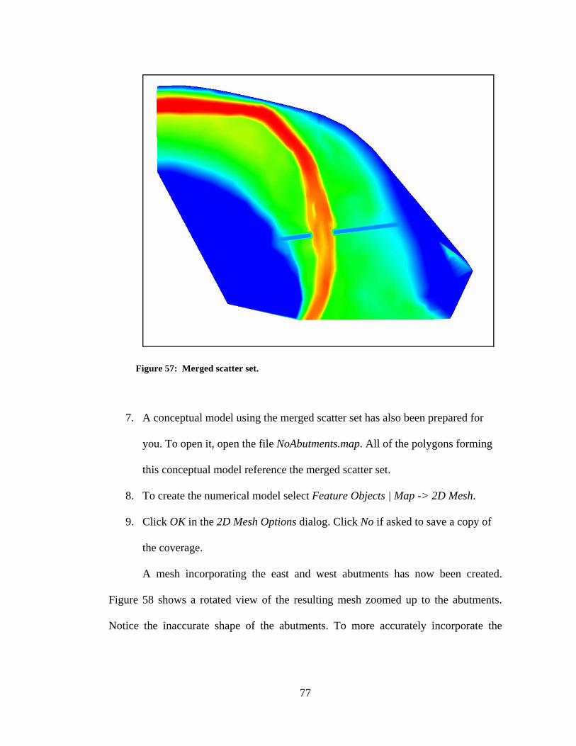
Figure 57: Merged scatter set.

7. A conceptual model using the merged scatter set has also been prepared for

you. To open it, open the file NoAbutments.map. All of the polygons forming

this conceptual model reference the merged scatter set.

8. To create the numerical model select Feature Objects | Map -> 2D Mesh.

9. Click OK in the 2D Mesh Options dialog. Click No if asked to save a copy of

the coverage.

A mesh incorporating the east and west abutments has now been created.

Figure 58 shows a rotated view of the resulting mesh zoomed up to the abutments.

Notice the inaccurate shape of the abutments. To more accurately incorporate the

77

abutments into a mesh, the coverages of the stamped features must be used to guide

the mesh around the abutments and to describe how to mesh the abutments.

Figure 58: Mesh incorporating the east and west abutments using Method 1.

Method 2: To use just the coverage of the stamped feature as part of the

conceptual model, it must be merged with the conceptual model. The merged

conceptual model must then be modified to properly include the stamped feature.

When using just the coverage of the stamped feature, it is used to simply outline the

extents of the stamped feature. Elements are created within the outline of the feature.

These elements get their elevation values from the existing bathymetry. Then these

elements are disabled so all water must flow around them. The interface between the

disabled elements and the enabled ones forms a vertical wall just like the open

78

boundaries of the model. Therefore, features integrated into numerical models by this

method are called vertical-walled features. Another way to integrate vertical-walled

features is to mesh around them. The advantage of disabling elements inside a

stamped feature is that solutions without the stamped features (elements enabled) and

solutions with the stamped features (elements disabled) can be opened onto the same

mesh. This is because the number of nodes and elements remain the same. Finite

difference grids can similarly use vertical-walled features for disabling cells.

Method 2 is also a quick method of integrating features into a numerical

model. With this method, you can control how the mesh goes around the stamped

features; however, water can never flow over the stamped features. Therefore, if the

water is deep enough to overtop the features, then Method 3 should be used.

To integrate abutments into a numerical model using this method:

1. While pressing CTRL select the No Abutments, West Abutment and East

Abutment coverages in the Project Explorer.

2. Right-click on the No Abutments coverage in the Project Explorer and select

the Merge Coverages menu item. Click No if asked to delete the coverages

making up the merged coverage.

3. Click on the Merge coverage item in the Project Explorer to active it.

4. Select Feature Objects | Clean to clean the merged coverage. Click OK in the

Clean Options dialog.

5. With the merged coverage cleaned, it can now be modified to incorporate the

stamped feature. This has already been done for you. To open the merged

coverage, open the file Merged.map. Figure 59 shows the merged conceptual

79

model. All the polygons on this conceptual model are tied to the existing

bathymetry scatter set.

Figure 59: Merged conceptual model.



the coverage.

A mesh incorporating the east and west abutments as vertical-walled features

has now been created. Figure 60 shows the plan view of the resulting mesh.

80


Method 3: The final method of integrating stamped features into a numerical

model uses both the scatter set of the stamped feature and the coverage of the stamped

feature. This method gives the modeler full control of how the stamped feature is

meshed and how the mesh goes around the stamped feature. Therefore, Method 3 is

the most time consuming. The structure of finite difference grids makes it impossible

to accurately align cell edges with changes in slope around stamped features.

Therefore, Method 3 is not applicable for use with finite difference grids.

Integrating the abutments into a numerical model using this method is very

similar how the abutments are integrated using Method 2. The coverage of the

81

stamped feature is merged with the conceptual model. The merged coverage is cleaned

and modified to integrate the abutments appropriately. The polygons making up the

abutments are linked to the merged scatter set rather than that of the existing

bathymetry.

To create a numerical model using Method 3:

1. Open the file Abutments.map.



the coverage.


82

A mesh incorporating the east and west abutments has now been created.

Figure 61 shows a rotated view of the resulting mesh zoomed up to the abutments.

Conclusion

This concludes the tutorial. You may continue to experiment with the SMS

interface or you may quit the program. To quit SMS at this point:

• Select File | Exit. If prompted to confirm, click the Yes button.

83

References

1. Christensen, J. R. (2001). Stamped Features: Automatic Generation of Flow

Modifying Structures in Conceptual Models. Thesis, Brigham Young

University.

2. Zundel, Alan K. and J. Ryan Christensen, “Stamped Features: Creation of

Engineered Structures in Conceptual Models”, International Journal of

Hyrdroinformatics, Vol. 4, No. 1, February 2002, pp. 63-72.

3. Zundel, A.K., Demirbelek, Z., Fugal, A.L., Jones, N.L, “Automatic Definition

of Two-dimensional Finite Element Coastal Models”, Proceedings of the Third

International Conference on HYDROINFORMATICS, Copenhagen, Denmakr,

Aug. 24-26, 1998.

4. Norman L. Jones, and David R. Richards, “A Conceptual Model Approach to

Hydroinformatics”, Proceedings of the Second International Conference on

HYDROINFORMATICS, Zurich, Switzerland, Sept. 9-13, 1996.

5. Nelson, E. James, Glenn E. Moglen, and Larry Arneson, “Building GIS

Database to Support Hydrologic Modeling at the Maryland State Highway

Administration”, Proceedings of the 78th Annual Meeting of the Transportation

Research Board, January 10-14, 1999, published on CD-ROM.

85

6. Gonzales, D. S. (2000). An Automatic Finite Element Mesh Generation

Method: The Adaptive Rectangular Coons Patch. Thesis, Brigham Young

University.

7. Nelson, E. James, and Norman L. Jones, “Reducing Elevation Roundoff Errors

in Digital Elevation Models”, Journal of Hydrology, July 1995, Vol. 169, pp.

37-49.

8. Nelson, E. James, Norman L. Jones, and Russell J. Berrett, “Adaptive

Tesselation Method for Creating TINs from GIS Data”, ASCE Journal of

Hydrologic Engineering, Vol. 4, No. 1, January 1999.

86

refining and expanding the feature stamping process

Documents