REFLECTION SEISMOLOGY: A BASIC INTRODUCTION

Tom Wilson January, 2003

TIME DISTANCE RECORDS BASIC DATA The in-class seismograph demo data were collected in a manner similar to an actual seismic survey. While we used only a simple 12 twelve channel seismograph and the recording used single phones (i.e. no geophone groups), it was illustrative of the basic acquisition approach. A shot is detonated at some point (or points to form a source array) and phones are distributed on the surface to record the different arrivals. Phones can be distributed across the surface in several different ways but the crucial data for any phone is its offset distance. Where was the phone relative to a given shot? Shot detonation initiates recording on the seismograph. Ground motion sensed by each phone or group of phones is passed to the seismograph and stored. Ground motion is sampled at constant time intervals referred to as the sample rate. The raw data recorded on the seismograph consists of a number recorded at a certain time that describes in a relative sense the motion of the ground at that instant of time. As noted in the demo, the basic data may be measurement of surface velocity, acceleration or pressure. These parameters vary with direction. In land surveys, measurements are usually made of the vertical component of surface velocity or acceleration. If multi-component phones are used then these measurements are made in 3 separate orthogonal directions.

Di TR

besim

agram of simple in-line 12 phone receiver string

AVEL PATHS What is recorded by the geophone and when it is recorded depends on what lies

neath the surface. What happens and when it happens is easily illustrated using a ple single-layer model for starters (below).

2

The 12-channel in-line receiver string sits at the surface to the right of the shot. First imagine what must happen. When will the mechanical disturbance generated by the shot jiggle the geophones? There are different paths along which the mechanical disturbance can travel. What are they?

Direct arrival How long will it take to get to a phone?

Reflected arrival How long will it take to get to a phone?

Critically refracted arrival How long will it take to get to a phone?

3

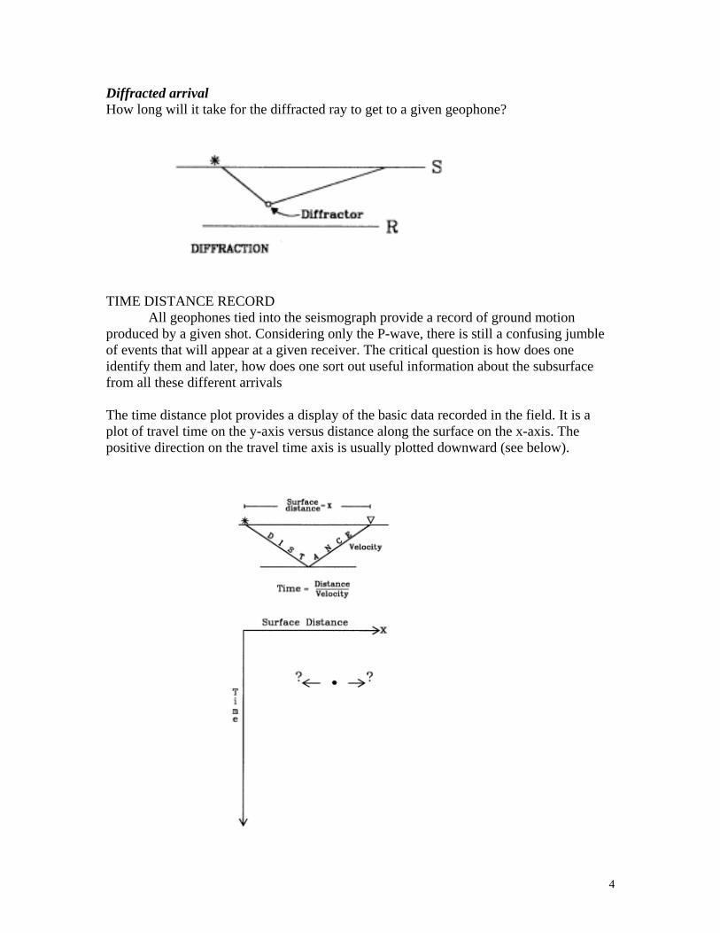
Diffracted arrival How long will it take for the diffracted ray to get to a given geophone?

TIME DISTANCE RECORD

All geophones tied into the seismograph provide a record of ground motion produced by a given shot. Considering only the P-wave, there is still a confusing jumble of events that will appear at a given receiver. The critical question is how does one identify them and later, how does one sort out useful information about the subsurface from all these different arrivals The time distance plot provides a display of the basic data recorded in the field. It is a plot of travel time on the y-axis versus distance along the surface on the x-axis. The positive direction on the travel time axis is usually plotted downward (see below).

4

Time distance axes. Where do you think the different events will appear?

In the t-x plot, the direct arrival forms a straight line with zero intercept and slope equal to the reciprocal of the interval velocity at the surface. The reflection event: A hyperbola

5

The critical refraction: a straight line tangent to the reflection.

The diffraction event: another hyperbola.

These different events get thrown together into a jumbled mess that doesn’t look much like a geologic cross section. It’s not easy to interpret subsurface geology from such a diagram. What’s a geologist to do? Things get even more complicated. WHAT ABOUT GROUND ROLL? In the above examples, we have only diagrammed the p-wave arrivals. Ground roll refers to the Rayleigh wave mentioned earlier. It is a real noise maker and acquisition and

6

processing efforts have to consider how to minimize its affect on data quality. It cuts through the reflection events that every interpreter wants to see clearly.

REAL DATA The situation becomes even more complex when you consider the presence of multiple layers. The shot record below is from a shallow seismic survey using the equipment we demonstrated in class.

7

The record below is from a Vibroseis survey conducted to image deeper stratigraphy and structure within the Appalachian foreland area.

SHOOTING GEOMETRY In the above example we used what’s referred to as an off-end source-receiver layout. One can also shoot using a split-spread layout or an asymmetrical split-spread layout. These different shooting geometries are illustrated below.

The reflection path geometry and reflection point coverage obtained in a simple six geophone split spread is illustrated below. In the diagram below, note that the spacing between reflection points is ½ the geophone spacing.

8

WHAT HAPPENS WHEN THE LAYER DIPS? This is illustrated best using the split-spread layout. The first diagram (below) illustrates how reflections travel down and back to the receivers over the horizontal interface. Note that the paths are symmetrical about the shot and that the time-distance plot portrays a hyperbola that is also symmetrical about the shot.

When tdip. Th

he layer dips (below), notice how the travel paths are shorter up-dip than down-e pattern is asymmetrical in space and time.

9

In the time-distance plot we still have the hyperbola, but its apex is offset in the up-dip direction.

We said it wobecomes eveso that an intis common m

uld get more complicated, and that question – “What’s a geologist to do?” n more critical. Common midpoint sorting and stacking simplifies the data erpreter can look at it and begin to make geologic sense out of it. But – what idpoint sorting?

10

COMMON MIDPOINT SORTING When you go through the simple exercise of drawing in the reflection travel paths from source to receiver in the layout and you see that the reflection points are equally spaced along the flat reflection surface at intervals equal to half the geophone spacing. To make things even simpler, lets take a look at what happens for a 6-phone string. Draw in the reflection points and label them 1 through 6 across the bottom below the reflecting interface. Now move the shot to the right over to the location of the first phone on the string and take that phone and move it out to the end. Maintain the geophone interval. Draw in the reflection travel paths again and note that they reflect from some of the same points of reflection associated with the first shot. Label those reflection points with the appropriate phone number. Keep moving the shot and geophone string along to the right and notice the pattern that builds up in the phone numbers that label each reflection point. They begin repeating, and notice that in this setup there are never more than three source receiver combinations that provide information about a given reflection point.

In this flat layer example, note that the three source-receiver combinations that provide information from a single reflection point share the same surface midpoint (see below).

11

They also have the same reflection point. Based on these relationships, this arrangement of sources and receivers has come to be known as common midpoint (CMP) or common depth point (CDP). You may recall hearing of CDP data or CMP data in your structure or petroleum geology class. That is just a reference to these geometrical interrelationships. If we extract only those traces that share a common midpoint we have what is called a common midpoint “gather.” The process of sorting out (or extracting) records that share a common midpoint is called common midpoint sorting. What happens when we put some dip into the reflecting layer and go through this process of sketching in the reflection travel paths? After all, this is the more general and more realistic case. The source receiver combinations still retain the common midpoint, but they do not reflect from a common depth point on the dipping interface. Note that the reflection points walk up dip as the offset increases and none of the reflection points lie beneath the midpoint. For this reason these data are more appropriately referred to as common midpoint data than as common depth point data. Note that image points are used to identify the reflection point.

What does the time distance plot for the common midpoint reflection record look like? In the flat layer case we have another hyperbola that looks just like the one we had for the shot record. Distances are still source-to-receiver distances, but there is no common reference point as there was in the case of the shot record. Each reflection has a different receiver and source location.

12

What about the appearance of the dipping layer reflection in the CMP gather? Recall that the dipping layer response of the shot record yields a hyperbola, but the apex of the hyperbola is displaced up dip. Source-receiver combinations sharing a common midpoint depicted above reveal that when the reflecting layer dips, the reflection points do not coincide. As the source-receiver offset increases, the reflection point actually moves higher up the dipping layer. Hence, information recorded on separate source-receiver combinations arises from different but adjacent points on the reflecting layer. A useful characteristic of the common midpoint record is that whether the layer is dipping or not, we always get a hyperbola whose apex is centered at 0-offset (as shown above). This is very important because of what is done next to the CMP data set. Definition - CMP Gather: A collection of traces sharing a common midpoint.

NORMAL MOVEOUT CORRECTION The first thing a geologist wants to do when they see a shot record or CMP gather is to straighten out the reflection events. (The reflections are from the same or nearby reflections points – so they should all arrive at the same time.) In the simplest case - that for the horizontal reflector - the hyperbolic increases in travel time from short to long offsets are due only to the increasing distance of the source from the receiver. We want to see geologic changes – actual changes in the shape of the layer not ones due to changes in the locations of sources and receivers at the surface. The increase you see in arrival time (or travel time) with offset is called moveout. Take a minute and consider the diagram below showing the reflection travel paths in the common midpoint gather. Next to it is the simple hyperbolic reflection event we would expect to see. And if we shot back (to the left) as well as forward (to the right) we could show both halves of the hyperbola.

13

The reflections all come from the same point. If the source and receiver were sitting right on top of each other then the wave would travel straight down and back up to the surface. This is the shortest possible travel path. The record would make more sense to us – geologically speaking – if all the arrivals came in at the same time. To do this, we need to shift all the arrival times so that they “appear” to have gone straight down and back up to the surface.

Making that shift is referred to as making the moveout correction and the difference from the “zero-offset” travel time and the actual travel time is called the moveout. To make the moveout correction we simply compute the moveout (∆tX1 or ∆tX2, below) and subtract it from the actual arrival time. The correction is often referred to as the NMO (normal moveout) correction.

14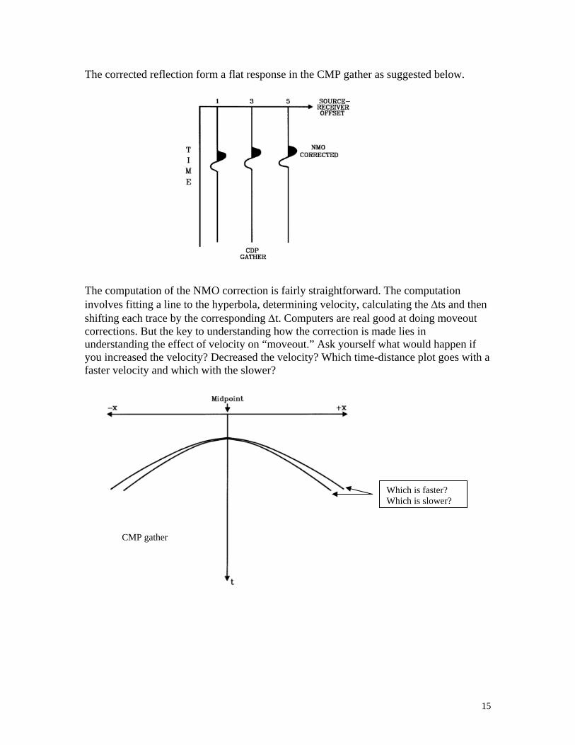

The corrected reflection form a flat response in the CMP gather as suggested below.

The computation of the NMO correction is fairly straightforward. The computation involves fitting a line to the hyperbola, determining velocity, calculating the ∆ts and then shifting each trace by the corresponding ∆t. Computers are real good at doing moveout corrections. But the key to understanding how the correction is made lies in understanding the effect of velocity on “moveout.” Ask yourself what would happen if you increased the velocity? Decreased the velocity? Which time-distance plot goes with a faster velocity and which with the slower?

CMP gather

Which is faster? Which is slower?

15

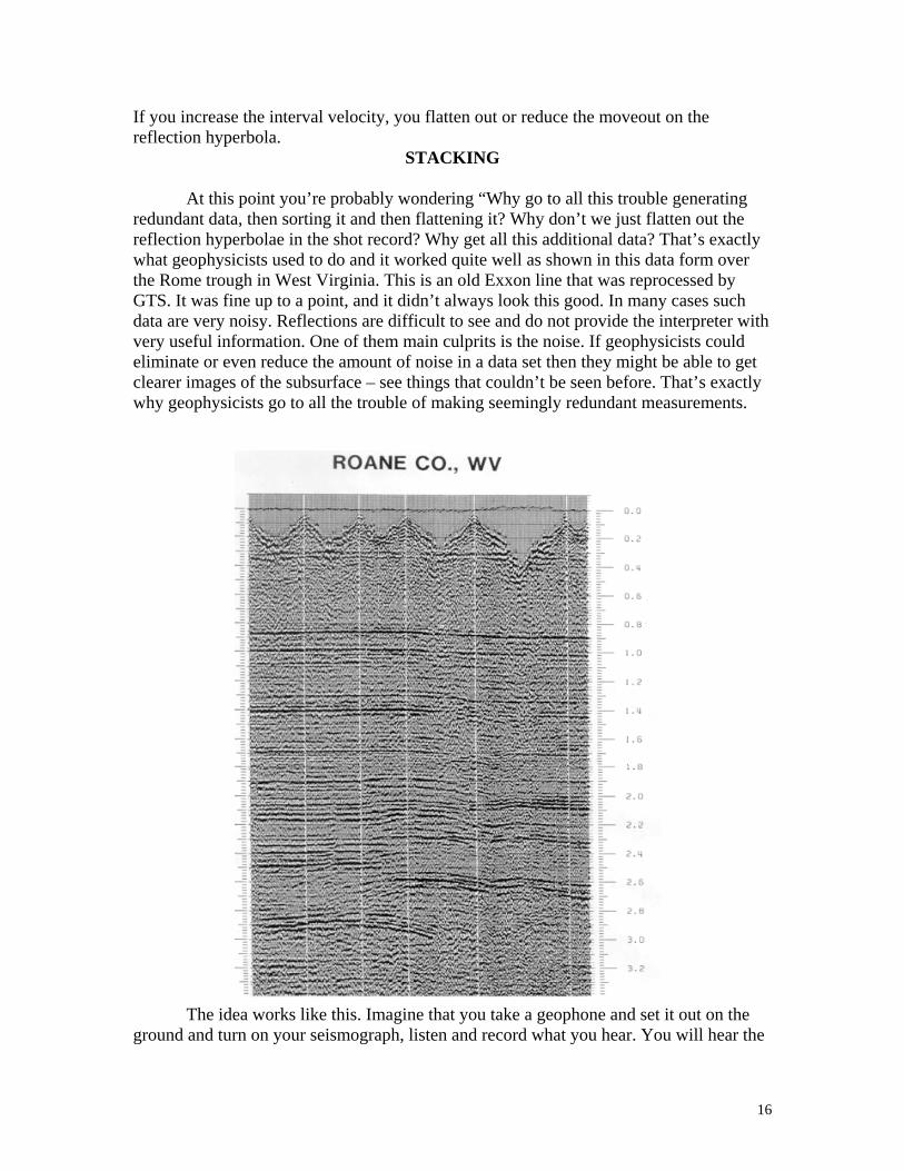
If you increase the interval velocity, you flatten out or reduce the moveout on the reflection hyperbola.

STACKING At this point you’re probably wondering “Why go to all this trouble generating redundant data, then sorting it and then flattening it? Why don’t we just flatten out the reflection hyperbolae in the shot record? Why get all this additional data? That’s exactly what geophysicists used to do and it worked quite well as shown in this data form over the Rome trough in West Virginia. This is an old Exxon line that was reprocessed by GTS. It was fine up to a point, and it didn’t always look this good. In many cases such data are very noisy. Reflections are difficult to see and do not provide the interpreter with very useful information. One of them main culprits is the noise. If geophysicists could eliminate or even reduce the amount of noise in a data set then they might be able to get clearer images of the subsurface – see things that couldn’t be seen before. That’s exactly why geophysicists go to all the trouble of making seemingly redundant measurements.

The idea works like this. Imagine that you take a geophone and set it out on the ground and turn on your seismograph, listen and record what you hear. You will hear the

16

earth creek and groan as cars drive by, as the wind blows, rain falls, water flows by in the stream, as a cow steps on your geophone, etc. All these things happen more or less at random. If you repeat this experiment you will get another record that will be completely different from the first. If you were listening for a reflection to make its way back to the surface this noise just gets in the way. It’s like listening to a faint signal on the radio. The noise or “static” could be so loud that you never hear your reflection. Now, as another experiment, assume that rather than just listening to the noise, that you bang on the ground and listen for a reflection from some layer you know is there. If there were no noise it would come in at some time. The ground would wiggle up and down as the wave made its way back to the surface (see A below). But in reality, there is a lot of noise there. You might not have been able to pound as hard as you would have liked. Perhaps you wanted to use 50 pounds of dynamite but the local landowners would only let you use a couple ounces. Instead you keep hitting the ground and making records that you save. On any one record you can’t see the reflection event very well – if at all. But- if you sum them together – then what happens? The reflection always arrives at the same time. What about the noise? The noise vibrations, if they are random, will jiggle the phone in one direction during the first recording and then in another different direction during the next. It is very unlikely that random vibrations of the ground will shake the phone in the same direction during subsequent recordings. When several recordings are summed together, the noise gets smaller and smaller in amplitude. Noise vibrations at one time partially cancel those recorded at another time. The signal, on the other hand, continues to build in amplitude in direct proportion to the number of records that are summed together. Sometimes the noise can be coherent as in the case shown below. In this example, seismic recordings were made over an underground longwall mining operation.

17

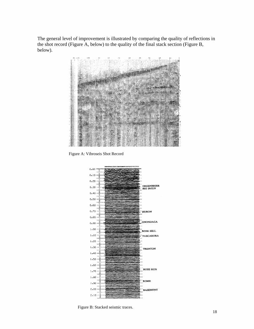
The general level of improvement is illustrated by comparing the quality of reflections in the shot record (Figure A, below) to the quality of the final stack section (Figure B, below).

18Figure B: Stacked seismic traces.

Figure A: Vibroseis Shot Record

FOLD In the stacking chart diagram shown previously (see also below) for the simple 6-phone geophone array, three reflection observations are obtained from each midpoint. This is the maximum number of records or observations that can be obtained of that reflection point with this acquisition geometry. That number of records, the maximum number of records of a given reflection point, obtained from the common midpoint gather of traces is referred to as the “fold”. In this simple example, 3 is the maximum “fold” of the data. On the ends of the profile the fold increases from 1 to the maximum of 3. The fold then remains constant until the right end of the profile is reached.

Uvsre

nlike the fold in this simple example, the fold along a seismic line can often vary. These ariations occur because of bends in the road (see figure below). They can also occur in traight “cross country” lines when rivers or other barriers result in gaps in the shooting, cording or both.

19

The problems of sorting into common midpoint bins can become complicated by the line geometry as shown in the more realistic example below..

SIGNAL TO N As noted in thequality and amdegree of enhaThis ratio is difold is increaseThis problem w“random” walktake the walkeanecdotally in the stumbler gesquare-root of cannot be elimcompromise be In the eobtained from

Along crooked survey lines, the common midpoint gatherincludes all records whose midpoints fall within a certain radius of some point

OISE RATIO

discussion of stacking, the redundancy of observations helps improve the plitude of the signal while minimizing the deleterious effects of noise. The ncement is described quantitatively in terms of the signal to noise ratio. rectly proportional to the square root of the fold of the seismic data. If the d from 1 to 4 then the signal to noise ratio is increased by a factor of 2. as originally solved by Einstein and is often described in terms of a . The random walk poses the question – “ will a series of random steps

r somewhere other than their starting point?” The problem is often posed the form of the drunken sailor experiment. The common expectation is that ts nowhere, but in fact the stumbler makes progress proportional to the

the number of steps taken. Noise can be attenuated but - if truly random - inated entirely. The decision of what fold to use is often based on a tween data quality and economics. xample shown below, note the improvement in reflection continuity stacking the noisy traces.

20

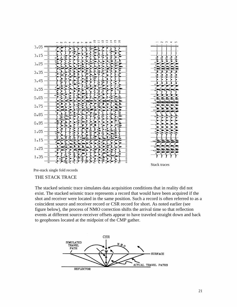
THE STACK TRACE

Pre-stack single fold records

Stack traces

The stacked seismic trace simulates data acquisition conditions that in reality did not exist. The stacked seismic trace represents a record that would have been acquired if the shot and receiver were located in the same position. Such a record is often referred to as a coincident source and receiver record or CSR record for short. As noted earlier (see figure below), the process of NMO correction shifts the arrival time so that reflection events at different source-receiver offsets appear to have traveled straight down and back to geophones located at the midpoint of the CMP gather.

21

When reflectors are flat the resulting seismic section (lower graph in figure below) accurately portrays “structural” information.

Reflection events appearing on a CSR record appear as though they have traveled down to the reflector point and back along a path which is normally incident on the reflector, as shown above. However, reflectors are often deformed into complex structures, and the depositional patterns, themselves, can give rise to complex variations in reflector geometry. The figure below portrays normal incidence reflections returned to a single , coincident, source and receiver point. In this example, there are only three normal incidence paths: one, down and back from point B and two others, down and back from points A and C.

22

For this reason, the coincident source-receiver record is also often referred to as a normal incidence record. As you can quickly appreciate, the events that appear on a normal incidence seismic record may not represent actual vertical relationships in depth beneath the midpoint (see below) since the reflection events do not originate from points directly beneath the midpoint or directly beneath the imaginary coincident source-receiver.

B

C

A

This can lead – particularly in areas of complex structure – to considerable distortion in the representation of subsurface structure and structural interrelationships. The relationships implied by the names: coincident source and receiver record or normal incidence record, are useful too understanding the nature of the data presented in this type of record. However, the reference you are most likely to encounter when talking to seismic interpreters is that of the CDP stack section or CDP seismic section.

MODELING The paths along which reflection events travel are referred to as ray paths. The ray paths in the normal incidence seismic section are normal incidence ray paths. Processors do their best to eliminate the geometrical distortions appearing in the stack section using a process referred to as migration, which we will discuss later. Regardless of the confidence one has in the subsurface view provided by the seismic section it is often the case that more than one interpretation of the subsurface is possible. For this reason the interpreter like to generate model seismic surveys across their interpretations to see how

23

well the seismic expression of their geological interpretation matches actual seismic data across the area. The process of simulating the seismic response of the interpreter’s model requires knowledge of subsurface interval velocities and densities. Velocities and densities are obtained from sonic and density logs of a well that is preferably located near the area where seismic data is being acquired. Knowledge of velocity is necessary because the seismic section is basically a representation of the time it takes for seismic energy to travel down to a reflecting interface and back to the surface. Velocity and density are combined to provide a measure of the strength of the reflection. The measure of reflection strength is the reflection coefficient and its value

2 1

1 2

Z ZRZ Z

−=

+

where Z is acoustic impedance and is equal to the product ρV, where V represents interval velocity and ρ, interval bulk density. The subscripts refer to the layer number. R tells the interpreter how large the amplitude of a given reflection will be and also, how the reflection strength of a reflector from one interface will compare with that from another. The pool player learns early on to violate this law using “English” (placing a spin on the ball) (below left).

Only for pool players

The basic mathematical relationships governing how rays travel from source to receiver are the reflection and Snell’s laws. For reflection, the angle of incidence equals the angle of reflection (see figure below).

24

Snell’s law (see below) is one known very well by every spear fisherman. Because the velocity of light in water is less than that in air the fish appears beyond its actual location.

RAY TRACI The first stepis to computeBecause NMand receiver travel times iis one along Dipping Refaccurate reprof horizontalthe receiver frecord surfac

NG

in converting the interpreter’s subsurface representation into a seismic view travel times to and from the reflector(s) represented in the interpretation. O correction and stack simulate seismic data as it would appear if the source were located at the same point on the surface the calculation of two-way s simplified. As mentioned above, the coincident-source-receiver travel path which reflection takes place at normal incidence to the reflecting interface

lector Horizon: The coincident-source-receiver format of the data yields an esentation of subsurface structural interrelationships only for the trivial case layers as noted earlier. When the reflecting surface dips, ray paths travel to rom points up-dip (see figure below). The seismic image of the reflector (the e) suggests that the reflector is longer than actual and has less dip.

25

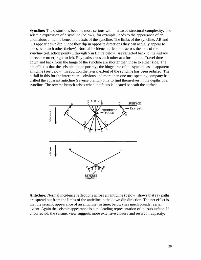
Syncline: The distortions become more serious with increased structural complexity. The seismic expression of a syncline (below), for example, leads to the appearance of an anomalous anticline beneath the axis of the syncline. The limbs of the syncline, AB and CD appear down dip. Since they dip in opposite directions they can actually appear to cross over each other (below). Normal incidence reflections across the axis of the syncline (reflection points 1 through 5 in figure below) are reflected back to the surface in reverse order, right to left. Ray paths cross each other at a focal point. Travel time down and back from the hinge of the syncline are shorter than those to either side. The net effect is that the seismic image portrays the hinge area of the syncline as an apparent anticline (see below). In addition the lateral extent of the syncline has been reduced. The pitfall in this for the interpreter is obvious and more than one unsuspecting company has drilled the apparent anticline (reverse branch) only to find themselves in the depths of a syncline. The reverse branch arises when the focus is located beneath the surface.

Anticlinare spreathat the sextent. Auncorrec

e: Normal incidence reflections across an anticline (below) shows that ray paths d out from the limbs of the anticline in the down dip direction. The net effect is eismic appearance of an anticline (in time, below) has much broader aerial gain the seismic appearance is a misleading representation of the subsurface. If ted, the seismic view suggests more extensive closure and reservoir capacity.

26

Fault: The seshown here (leading to divhorizon prodappears wide

Diffractions athe surface le

ismic expression of faulted horizons can be quite varied. The simple case see below) portrays normal offset of a layer accompanied by minor uplift erging dips on opposite sides of the fault. Reflections from the faulted

uce an apparent shift of horizon segments down dip. The apparent fault gap r than it actually is.

rising from faulted edges of the horizon (see figure below), fan out across ading to the appearance of hyperbolic events in the seismic section. These

27

diffractions may suggest the presence of rollover into the fault. In general the interpreter finds the diffractions helpful, since their apex accurately locates the position of the fault. A line drawn to connect the diffraction apex defines the location of the fault plane.

GEOMETRIC The above modTheir effect is COMPUTER G Seismic modelof the above exdeformed horizfrom velocity v15,000 feet per Syncline: Theexample. The cwe can. Note tof reflection evlower horizon

AL PITFALLS

els illustrate a few “pitfalls” that are classified as geometrical in nature. to distort the appearance of subsurface structure.

ENERATED MODELS

ing is routinely undertaken at the computer workstation. Computer models amples are shown below. A single flat layer has been added beneath the on in each of these models to illustrate additional distortions that arise ariation. In each model the velocity above the deformed horizon (Va) is second and that below (Vb), 20,000.

ray-tracing here (below) is much more thorough than in the preceding omputer can compute and draw these ray paths much more quickly than

he familiar features in the diagram including the buried focus and the travel ents from the reflector surface to receivers down dip. Reflections from the

are incident at right angles and return to the receiver along their downward

28

path. As the rays travel back to the surface they pass from the deeper high velocity layer into the lower velocity surface layer and are refracted toward a line drawn normal to the reflector surface.

In the time dbased on ousuggests thatoward the emedium thathrough the of the traveltime taken tless in propthe high velway down athe limbs ofwhich travethickness ofoccupying t

isplay (below) the reverse branch and crossing synclinal limbs are expected r previous discussion. However, the appearance of the underlying reflector t it may also have experienced a similar level of deformation. Ray paths dges of the model travel through a greater thickness of the higher velocity n do rays traveling down hinge area. While the lengths paths do not vary greatly, the o travel these different paths is ortion to the distance traveled in ocity layer. Rays make their nd back more quickly high on the syncline than do rays l through a much greater the low velocity medium he hinge area of the syncline.

29

Anticline: Computer ray tracing was performed acros the more complex anticlinal structure shown below. Based on the preceding discussion, we expect the reflections from the crest of the anticline to fan out and produce an anticline with much broader appearance in the time section. However, note that we have a tight syncline sitting between two anticlines.

Subsurface structural interpretation across the Summit Field north of Morgantown along the Chestnut Ridge anticline.

Raytracing through the syncline shown below shows that we have a buried focus

event, and what we should expect to see in time is another anticline – not a syncline.

30

Normal incident rays rising from the lower interface are refracted toward the normal in accordance with Snell’s law. Travel times to and from the underlying flat horizon (Figure) decrease below the anticlinal hinge and increase down the limbs taking on an anticlinal form.

Can you spot the reverse branch and apparent anticline arising from the base of the syncline?

31

VELOCITY PITFALLS Along with the class of geometrical pitfalls there are also pitfalls or distortions associated with subsurface velocity distribution. Did you notice anything unusual about the time section across the simple syncline in our first ray-tracing example (reproduced below)?

Reflections from the shallow syncline and deeper – flat – reflector.

The velocity in the layer beneath the synclinally shaped shallow reflector is much faster than in the overlying layer. Thus, two-way travel times to the deeper reflector on either side of the syncline arrive much earlier than do reflections from the same depth that travel through the axis of the syncline. Velocity distribution in the syncline model produces a “sag” in the reflection from the deeper flat horizon beneath the syncline, since the syncline contains a much thicker section of low velocity strata. The example below illustrates a combination of velocity and geometrical pitfalls inherent in the seismic time section. In this example, a seismic line crosses a reef.

32

The ray path diagram shown below suggests that the recordings of reflection travel times in the normal incidence format simulated by the CMP stack trace will be complicated and not directly related to the structural features portrayed in the depth section above.

33

How might the time section shown below, lead to incorrect interpretation of subsurface structure?

Seismic section over the reef.

SEISMIC WAVELETS, DECONVOLUTION AND STRATIGRAPHIC INTERPRETATION The seismic wavelet refers to the mechanical disturbance, generated by the seismic source that travels through the subsurface. The impact of a hammer produces a jolt of energy that passes quickly. A charge of dynamite when detonated rapidly deforms the surrounding area and sends out a shock wave which may be felt as a rapidly passing shake of the ground. It is the temporal characteristics of this pulse of deformation produced by the seismic source that we refer to as the seismic wavelet, seismic pulse, or just wavelet. An example of a seismic wavelet is shown below. Note that time plots left to right.

Wavelets come in many different shapes and sizes. Another wavelet is shown below.

Basic Seismic Wavelet

WAVELET A

34

Note that this wavelet is more compact or has shorter duration than the one above.

WAVELET B

Seismic data processing is a fascinating field of study. There are many techniques applied to seismic data that enhance the quality of the seismic image and help improve the resolution of subtle geological features – both structural and stratigraphic. One very important seismic data processing procedure is known as deconvolution. Deconvolution can be thought of as a pulse compression technique; in other words, it is a process applied to seismic data to reduce the duration of the seismic wavelet. It is a process which can transform wavelet A into wavelet B shown above. The benefits of deconvolution become evident when we think about resolving the top and bottom of a layer. If wavelet A is reflected back to the surface from the top and bottom of a reflective interval, note that the long duration of the reflection event from the top of the layer will probably overlap or interfere with the reflection from the base of the layer, making it difficult to distinguish between the two. Let’s take a look at some of the difficulties that can arise. Examine the section below – and before turning the page make an interpretation of this small seismic section.

Section A

The section above is actually a synthetic or model (made up) seismic data set. The structural and stratigraphic features in the model are representative of graben structures encountered in the North Sea. Note the obvious stratigraphic pinch-out. This would make a nice stratigraphic trap. Now take a look at the seismic section below.

35

Section B

What happened to that pinch-out? The geologic model of the area is shown below. The reflective properties of each layer are defined by the velocity contrasts shown in the cross section. This geologic model was transformed into the seismic displays shown above. The only difference between the two model seismic displays is in the wavelet that was reflected from the interfaces between layers. In the first seismic section, Wavelet A was used; in the second, Wavelet B.

Note that the Upper Jurassic Hot Shale and Callovian Shale are capped by a basal Cretaceous marl/limestone unit. A complex deformation history is revealed by the variations in thickness of the different units across the normal faults bounding the horst

36

and across the top of the horst-block itself. The Hot Shale and Callovian Shale do not pinch-out against the basal Cretaceous. So why does a pinch out appear in the Section A? Go back and take a close look at Wavelet A. This wavelet has a long duration; the first two cycles in the wavelet have relatively high amplitude. When this wavelet reflects from the basal Cretaceous interval across the top of the horst-block, the initial reflection is accompanied by all the cycles in the wavelet. (Wavelet A). In section A the follow cycles of the reflections from the basal Cretaceous follow beneath and drop with the reflector left to right across the horst-block; and as they do, they intersect the reflection event from the base of the Hot Shale and Callovian Shale. The result gives the illusion that these Jurassic shales pinch out againts the basal Cretaceous. When the seismic data is deconvolved (i.e. when wavelet A is transformed into wavelet B, the long tail is eliminated from the wavelet. Reflections in the deconvolved section (Section B) consist of a single sharp reflection event with no following cycles to complicate the appearance of the seismic section. Deconvolution produces significant improvement in the resolution of geologic features in the seismic section. However, even with this simplified, more compact wavelet, we are still faced with resolution limitations when the two-way travel times separating reflectors are less than the duration of the seismic wavelet. Overlap becomes a problem again, and we loose the ability to identify relatively thin layers. To sharpen your interpretation skills try your hand with the section below. On a separate

sCin

heet of paper sketch your interpretation of the geology producing this seismic response. an you find the sand channel? Can you find a velocity anomaly? Do stratigraphic tervals continue across the axis of the anticline?

37

38