WORKING PAPER SERIESFED

ERAL

RES

ERVE

BAN

K of A

TLAN

TA

Indeterminacy in a Forward-LookingRegime Switching Model Roger E.A. Farmer, Daniel F. Waggoner, and Tao Zha Working Paper 2006-19 November 2006

The authors thank Troy Davig, Jordi Galí, Eric Leeper, Julio Rotemberg, Tom Sargent, Chris Sims, Lars Svensson, Eric Swanson, Noah Williams, and Michael Woodford for helpful discussions. Farmer acknowledges the support of National Science Foundation grant #SES0418074. The views expressed here are the authors’ and not necessarily those of the Federal Reserve Bank of Atlanta or the Federal Reserve System. Any remaining errors are the authors’ responsibility. Please address questions regarding content to Roger E.A. Farmer, Professor, Department of Economics, University of California, Los Angeles, Box 951477, Los Angeles, CA 90095-1477, 310-825-6547, 310-825-9528 (fax), rfarmer@econ.ucla.edu; Daniel Waggoner, Research Economist and Associate Policy Adviser, Research Department, Federal Reserve Bank of Atlanta, 1000 Peachtree Street, N.E., Atlanta, GA 30309-4470, 404-498-8278, daniel.f.waggoner@atl.frb.org; or Tao Zha, Research Economist and Senior Policy Adviser, Research Department, Federal Reserve Bank of Atlanta, 1000 Peachtree Street, N.E., Atlanta, GA 30309-4470, 404-498-8353, tzha@earthlink.net. Federal Reserve Bank of Atlanta working papers, including revised versions, are available on the Atlanta Fed’s Web site at www.frbatlanta.org. Click “Publications” and then “Working Papers.” Use the WebScriber Service (at www.frbatlanta.org) to receive e-mail notifications about new papers.

FEDERAL RESERVE BANK of ATLANTA WORKING PAPER SERIES

Indeterminacy in a Forward-Looking Regime-Switching Model Roger E.A. Farmer, Daniel F. Waggoner, and Tao Zha Working Paper 2006-19 November 2006

Abstract: This paper is about the properties of Markov-switching rational expectations (MSRE) models. We present a simple monetary policy model that switches between two regimes with known transition probabilities. The first regime, treated in isolation, has a unique determinate rational expectations equilibrium, and the second contains a set of indeterminate sunspot equilibria. We show that the Markov switching model, which randomizes between these two regimes, may contain a continuum of indeterminate equilibria. We provide examples of stationary sunspot equilibria and bounded sunspot equilibria, which exist even when the MSRE model satisfies a generalized Taylor principle. Our result suggests that it may be more difficult to rule out nonfundamental equilibria in MRSE models than in the single-regime case where the Taylor principle is known to guarantee local uniqueness. JEL classification: E5 Key words: policy rule, inflation, serial dependence, multiple equilibria, regime switching

INDETERMINACYIN A FORWARD LOOKING REGIME SWITCHING MODEL

I. Introduction

Work by Richard Clarida, Jordi Galí and Mark Gertler (2000) has stimulated recentinterest in models where monetary policy may occasionally change between a passiveregime in which there exists an indeterminate set of sunspot equilibria and an activeregime in which equilibrium is unique. Models of this kind are inherently non-linearsince the parameters of the model are represented by elements of a Markov chain.

Papers in the literature on nonlinear rational expectations models typically com-pute a solution to functional equations using numerical methods, but not much isknown about the analytical properties of these equations. In an important paper,Lars Svensson and NoahWilliams (SW) (2005) have proposed an algorithm for solvingMarkov switching rational expectations (MSRE) models. Our computational experi-ments suggest that the SW algorithm will find the unique value of the minimum-state-variable (MSV) when it exists but it may also converge to one of a set of indeterminateequilibria (Farmer, Waggoner, Zha (2006, Appendix 2)). Obtaining a complete set ofindeterminate equilibria even for a simple MSRE model is a much more difficult prob-lem, and to the best of our knowledge there are no systematic methods to accomplishthis task.

The distinction between the linear RE model and the MSRE model is subtle butimportant and the conditions for existence and boundedness of a unique solution aredifferent in the two cases. In this paper we study a simple Markov-switching modelof inflation that combines two purely forward-looking rational expectations models.The first one has a unique determinate equilibrium and the second is associated witha set of indeterminate sunspot equilibria. The MSRE model switches between thetwo models with transition probabilities governed by a Markov chain.

Within the MSRE environment we first establish the existence of an MSV equi-librium for almost all values of the transition probabilities. We go on to discussalternative definitions of stationarity for non-linear models and we argue that mean-square stability is an appropriate and appealing concept. We then show through aseries of examples that there exists a set of mean-square-stable sunspot equilibria forlarge open sets of the model’s parameter values. Our results imply that the exis-tence of stationary sunspot equilibria in MRSE models is a pervasive phenomenonthat cannot be ruled out in all regimes by the actions of the policy maker in a singleregime.

1

INDETERMINACY 2

II. The Model

Following Robert King (2000) and Michael Woodford (2003), we study a simpleflexible price model in which the central bank can affect inflation but not the realinterest rate. In this model, the Fisher equation links the real interest rate, rt, andthe nominal interest rate, Rt, by the equation,

Rt = Et [πt+1] + rt, (1)

where Et is the mathematical expectation at date t and πt+1 is the inflation rate atdate t + 1. The central bank sets the time-varying rule

Rt = φξtπt − κξtεt, (2)

where ξt is a two-state Markov process with transition probabilities (pi,j) and pi,j isthe probability of transiting from state j to state i. The stochastic process {εt}∞t=1

is independently distributed with mean zero and unit variance and is independentof {ξt}∞t=1. Substituting Eq. (2) into Eq. (1) gives the following forward-lookinginflation process

φξtπt = Et [πt+1] + rt + κξtεt. (3)

We assume that the real interest rate evolves exogenously according to

rt = ρrt−1 + νt, (4)

where |ρ| < 1 and {νt}∞t=1 is independently distributed with zero mean and finitevariance and is independent of {ξt}∞t=1 and {εt}∞t=1.

III. An Appropriate Equilibrium Concept

Much of the previous work on dynamic stochastic general equilibrium theory hasbeen concerned with constant parameter models. A typical way to proceed is tospecify preferences, technology and endowments and to make an explicit assumptionabout the nature of stochastic shocks. Sometimes it is possible to specify an envi-ronment in which, in the absence of shocks, there exists a unique stationary perfectforesight equilibrium. An example is the single agent real business cycle model. Whenthe stationary equilibrium is unique it may be possible to approximate a stochasticrational expectations equilibrium by linearizing the non-stochastic model around thesteady state and solving for an approximate stochastic rational expectations equi-librium. For this solution to be asymptotically valid the stochastic shocks must bebounded. Boundedness is necessary to keep the system close to the non-stochasticsteady state - the only point in the state space for which the linear approximation isexact.

The non-stochastic dynamics of a perfect foresight linear model are completelycharacterized by the roots of the characteristic polynomial of a first order matrixdifference equation. When all of these roots lie within the unit circle, the stochasticprocess is stationary and, as a consequence, it is possible to prove theorems which

INDETERMINACY 3

assert that as the variance of the shocks goes to zero, the approximation error vanishes.One would like to prove a similar theorem for the Markov switching model but sincethe model is inherently non-linear, this is impossible. To make progress with modelsof this kind one needs an appropriate equilibrium concept different from that used forlinear RE models. Specifically, one would like to describe solutions that are stationaryin a Markov-switching model. In this paper we adopt a solution that is widely usedby engineers and control theorists, that of mean square stability.1

IV. Determinate and Indeterminate Solutions and the TaylorPrinciple

In single regime models there is a simple test for uniqueness that involves countingunstable roots and nonpredetermined variables.2 Rational expectations equilibriumis unique if the number of non-predetermined variables is equal to the number ofunstable roots. This root counting condition lies behind the Taylor principle; thatmonetary equilibrium will be locally unique if the central bank follows a monetarypolicy in which it raises the interest rate in response to inflation with a responsecoefficient greater than one in absolute value.

In an innovative paper, Troy Davig and Eric Leeper (2005, 2006) have tackled thequestion of how to think about indeterminacy in models of regime switching. Theiridea is to find a condition, similar to the Taylor principle, that applies to MSREmodels. Davig and Leeper define determinacy to mean the existence of a uniquebounded solution to a stochastic linear system. By imposing the restriction that theinterest rate coefficient of the Taylor rule must be positive, they find a conditionthey call a ‘long-run Taylor principle’ that involves a combination of interest rateresponse coefficients and transition probabilities. If this condition holds there existsa unique bounded equilibrium. If it fails there may be multiple equilibria driven bynon-fundamental shocks.

We have two criticisms of the Davig-Leeper result. First, we think the positiv-ity restriction is not merely for mathematical convenience, but rather an indicationthat there does not exist in general an equivalence between the existence of a uniquebounded equilibrium for a MSRE model and the generalized Taylor principle derivedfrom the linear RE counterpart. Economically, even if one believes that it is ap-propriate for a benevolent policy maker to choose a positive value for the interestrate response coefficient to inflation in the Taylor rule, one still cannot rule out thepossibility that an incompetent or ill-informed policy maker might react differently.Moreover, Rotemberg and Woodford (1999a, Page 83) have shown that the optimalTaylor rule may involve a negative value of this parameter. In Section VII we exploit

1The reader is referred to Costa Fragoso and Marques (2004). For linear models, one should notethat mean square stability is the same as the conventional definition of stationarity.

2As Sims (2001) points out, this test does not always work and the exact condition is morecomplicated.

INDETERMINACY 4

the fact that one or more regimes may be associated with a negative value for the in-flation response coefficient to provide an example where there exist multiple boundedsunspot equilibria even when the generalized Taylor principle is satisfied.

Second, we think that the boundedness criterion is too strong. To see why, notethat stationarity and boundedness are equivalent for a stochastic linear system whenall the shocks are restricted to be bounded. In practice, the distributions of the shocksare often assumed to be unbounded (e.g., normal or gamma distributions). But aslong as the stochastic process is stationary, the approximation around the steady stateremains reasonable. Similarly, the mean-square-stable process for a Markov-switchingmodel is stable around the steady state, which is what one needs for reasonableapproximations to the underlying economic environment.

V. The MSV Solution

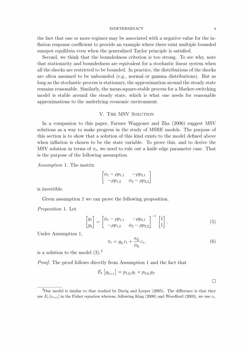
In a companion to this paper, Farmer Waggoner and Zha (2006) suggest MSVsolutions as a way to make progress in the study of MSRE models. The purpose ofthis section is to show that a solution of this kind exists to the model defined abovewhen inflation is chosen to be the state variable. To prove this, and to derive theMSV solution in terms of πt, we need to rule out a knife edge parameter case. Thatis the purpose of the following assumption.

Assumption 1. The matrix[φ1 − ρp1,1 −ρp2,1

−ρp1,2 φ2 − ρp2,2

]

is invertible.

Given assumption 1 we can prove the following proposition.

Proposition 1. Let[g1

g2

]=

[φ1 − ρp1,1 −ρp2,1

−ρp1,2 φ2 − ρp2,2

]−1 [1

1

]. (5)

Under Assumption 1,πt = gξtrt +

κξt

φξt

εt, (6)

is a solution to the model (3).3

Proof. The proof follows directly from Assumption 1 and the fact that

Et

[gξt+1

]= p1,ξtg1 + p2,ξtg2.

¤3Our model is similar to that studied by Davig and Leeper (2005). The difference is that they

use Et [rt+1] in the Fisher equation whereas, following King (2000) and Woodford (2003), we use rt.

INDETERMINACY 5

It follows from Theorems 3 and 4 in Farmer Waggoner and Zha (2006) that Eq.(6) is also the MSV solution. Following standard usage in the probability literatureon Markov switching models (e.g., Costa Fragoso and Marques (2004)), we definestationarity to be the existence of limiting first and second moments and it followsdirectly from Proposition 1 and the stationarity of rt and εt that the MSV solutionis stationary.

Definition 1 (Mean Square Stability). A stochastic process {xt}∞t=1 is mean squarestable if there exist real numbers µ and ϕ such that

lims→∞

Et [xt+s] = µ,

lims→∞

Et [x2t+s] = ϕ.

Mean square stability is stronger than the existence of a finite limit of first mo-ments and it is the appropriate stability concept if one wants to conduct statisticalinference. It is widely used in the engineering literature and has been used in an eco-nomic application, among others, by Svensson and Williams (2005). An alternativeto mean square stability is covariance stationarity in the sense of Hamilton (1994),or asymptotic covariance stationarity – a slightly weaker condition. Asymptotic co-variance stationarity implies mean square stability, although the converse is not truein general. However, for the class of solutions studied in this paper, Theorem 3.33of Costa Fragoso and Marques (2004) implies that these two notions are equivalent.Because of this fact, we will refer to solutions that satisfy the mean-square stabilitycriterion as “stationary”.

Proposition 2. The MSV solution (6) is stationary.

Proof. The proof follows directly from Definition 1. ¤Since the MSV solution exists for all the values of transition probabilities that

satisfy Assumption 1, it does not depend on the ergodic nature of transition proba-bilities.

VI. A Class of Indeterminate Solutions

Since the existence of a unique determinate solution is often viewed as a desirablefeature of a model (Rotemberg and Woodford (1999b), King (2000)), we address thequestion: Is the MSV solution (6) unique in the class of all stationary solutions?Often the answer to this question is negative and we illustrate this point by firstconstructing a class of indeterminate solutions with the condition lim

s→∞Et [xt+s] < ∞

as in the linear RE case. In the next section, we restrict solutions to stationary onesonly. Our example is instructive since it suggests that the idea that MSRE modelsare either determinate or indeterminate may not be fruitful.

Our model contains two state variables, πt and rt. However, all of the equilibria thatwe are interested in can be summarized a by a linear combination of these variables,

INDETERMINACY 6

defined as follows;4

xt = πt − gξtrt. (7)

Proposition 1 and Eq. (7) allow us to make the following change of variables.

Proposition 3. The inflation equation, Eq. (3), is equivalent to the following trans-formed equation in the variable xt,

xt =1

φεt

Et [xt+1] +κξt

φεt

εt. (8)

Proof. See Appendix 3. ¤

Rearranging Eq. (8), one can write the following expressions for xt+1 and Et [xt+1],

xt+1 = φεt

(xt − κξt

φεt

εt

)+ ηt+1, (9)

Et [xt+1] = φεt

(xt − κξt

φεt

εt

), (10)

where ηt+1 is an expectational error such that Et [ηt+1] = 0.Next, we make an assumption that characterizes the kind of central banker that

acts in each regime. The idea is that the policy maker in regime 1 is an inflation hawkand the policy maker in regime 2, an inflation dove. In line with the existing literatureon the Taylor principle, we do not assume that the inflation response coefficients, φ1

and φ2, must be positive.

Assumption 2.|φ1| > 1 > |φ2| > 0.

Assumption 2 implies that the two separate single-state models, where φξt = φi

for all t, have different determinacy properties. If we impose the assumption that asolution must satisfy the additional boundary condition,

lims→∞

Et [xt+s] = µ < ∞, (11)

then the linear model with φξt = φ1 has a unique solution represented by the equation

xt =κ1

φ1

εt, (12)

and the linear model with φξt = φ2 is associated with a continuum of indeterminatesunspot solutions of the form,

xt = φ2xt−1 − κ2εt−1 + γt, (13)

4Since rr is exogenous and stationary, and since we assume that ξt is ergodic and that gξtxt isuncorrelated with rt, xt will be stationary if and only if πt is stationary. Although we will workwith xt directly, the reader should bear in mind that the behavior of the inflation variable πt can berecovered from Eq. (7).

INDETERMINACY 7

where {γt}∞t=1 is an independent stochastic process with zero mean and finite variancethat is independent of {νt}∞t=1 and {ξt}∞t=1.

5

Definition 2. A mean zero stochastic process {ηt+1}∞t=1, and an initial condition x1

generate a solution to Eq. (8) if the sequence {xt+1}∞t=1 defined by Eq. (9) satisfiesthe condition

lims→∞

Et [xt+s] = µ < ∞.

Note that we define a solution to be a stochastic process with convergent firstmoments that satisfies Eq. (8) regime by regime and that transits between regimesaccording to the transition probabilities (pi,j). We now show how to construct alarge class of processes {{ηt+1}∞t=1 , x1} that generate solutions to Eq. (9) and thatare different from the MSV solution. We first rule out a pathological case in whichour result breaks down.

Assumption 3. The transition matrix satisfies the condition,

p2,2 > 0.

This assumption rules out the case where the second regime is a reflecting state.Define

x1 =

{κ1

φ1ε1 if ξ1 = 1,

x̄ ∈ R if ξ1 = 2.(14)

For t ≥ 1, define ηt+1 by

ηt+1 =

κ1

φ1εt+1, ξt = 1 and ξt+1 = 1,

γt+1 + κ2

φ2εt+1, ξt = 1 and ξt+1 = 2,

κ1

φ1εt+1 − φ2

(xt − κ2

φ2εt

), ξt = 2 and ξt+1 = 1,

γt+1 + κ1

φ1εt+1 + φ2

p1,2

p2,2

(xt − κ2

φ2εt

), ξt = 2 and ξt+1 = 2.

(15)

Since p2,2 > 0, the expectational errors {ηt+1}∞t=1 are finite. Note that time beginsat date 1 but the forecast errors begin with η2. We now state the main result of ourpaper.

Proposition 4. The pair {{ηt+1}∞t=1 , x1}, as defined in Eqs. (14) and (15), generatesa solution to Eq. (8) for any arbitrary zero mean sequence {γt+1}∞t=1. This indeter-minate solution takes the following form:

xt+1 =

{κ1

φ1εt+1, if ξt = 1 and ξt+1 = 1,

γt+1 + κ2

φ2εt+1, if ξt = 1 and ξt+1 = 2.

(16)

xt+1 =

{κ1

φ1εt+1, if ξt = 2 and ξt+1 = 1,

γt+1 + κ2

φ2εt+1 + φ2

p2,2

(xt − κ2

φ2εt

), if ξt = 2 and ξt+1 = 2.

(17)

5Note that γt could also be a function of εt and may or may not contain a component that isindependent of εt. Sunspot models of this kind are often interpreted as over-reaction to fundamentals.

INDETERMINACY 8

Proof. See Appendix B. ¤A solution consists of an initial condition and a rule for updating expectations; this

rule is implicitly defined by the endogenous shock process (15). Since the realizationof x1 is a function of the expectation, E1 [x2], the initial condition (14) imposed onthe realization of x1 is equivalent to the initial condition imposed on the expectationof x2. If ξt = 1, E1 [x2] = 0. If ξt = 2, the initial condition E1 [x2] does not constrainx1 and in this case, our definition of equilibrium picks an arbitrary initial condition,x̄.

The former discussion is informative because it suggests why the search for a globaluniqueness condition such as the generalized Taylor principle is unlikely to be suc-cessful. If the economy begins in state 1, the regime of the inflation hawk, the valueof inflation is pinned down by fundamentals. If instead the economy begins in state2, that is, if the inflation dove goes first, the initial value of inflation is unconstrainedand there exist multiple self-fulfilling paths. Since this simple model contains nolagged state variables there is no history to constrain actions; all behavior is purelyforward-looking and there is a sense in which the world begins again in every period.6

In regime 2 anything goes but, in regime 1, the economy must ‘snap back’ to a pointpinned down by fundamentals.

VII. Stationary Solutions

In this section we illustrate our results by providing two examples of indeterminatesolutions. The first example satisfies the mean-square stability condition so that thesolution is stationary. The second example satisfies the more restricted Davig-Leeperdefinition of a stationary equilibrium for which the stationary invariant distributionis bounded. In both examples, we show that the generalized Taylor principle fails tohold.

We begin with a general characterization of stationary solutions based on Proposi-tion 4 which implies that while in regime 2, xt will be serially dependent and governedby the process:

xt+1 =φ2

p2,2

(xt − κ2

φ2

εt

)+

κ2

φ2

εt+1 + γt+1. (18)

If∣∣∣ φ2

p22

∣∣∣ is less than one, xt will be stationary in regime 2.7 But even if∣∣∣ φ2

p22

∣∣∣ is greaterthan one, xt may still be globally stationary if the rate at which xt is increasing in thesecond regime is small relative to its expected duration. The following propositiongives the general condition for determining when xt is stationary.

6There may even be other equilibria of this model, that we have not explored, in which theexistence of an inflation dove permits non-fundamental shocks to hit the system even in the regimeof the inflation hawk.

7The assumption that a process is stationary in each regime is not enough to ensure overallstationarity. One can easily modify our example to produce a solution that is stationary for eachregime in isolation, but non-stationary for the system that allows regimes to switch.

INDETERMINACY 9

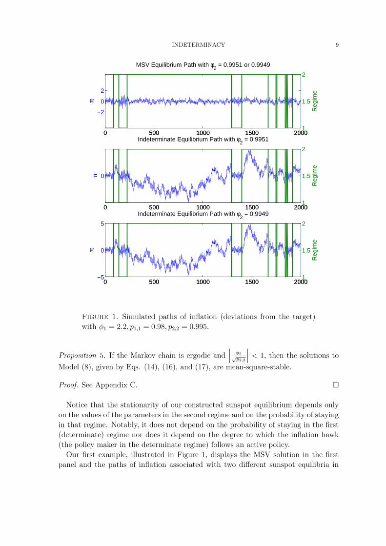
0 500 1000 1500 2000

−2

0

2π

MSV Equilibrium Path with φ2 = 0.9951 or 0.9949

0 500 1000 1500 20001

1.5

2

Reg

ime

0 500 1000 1500 2000

0π

Indeterminate Equilibrium Path with φ2 = 0.9951

0 500 1000 1500 20001

1.5

2

Reg

ime

0 500 1000 1500 2000−5

0

5

π

Indeterminate Equilibrium Path with φ2 = 0.9949

0 500 1000 1500 20001

1.5

2

Reg

ime

Figure 1. Simulated paths of inflation (deviations from the target)with φ1 = 2.2, p1,1 = 0.98, p2,2 = 0.995.

Proposition 5. If the Markov chain is ergodic and∣∣∣ φ2√

p2,2

∣∣∣ < 1, then the solutions toModel (8), given by Eqs. (14), (16), and (17), are mean-square-stable.

Proof. See Appendix C. ¤

Notice that the stationarity of our constructed sunspot equilibrium depends onlyon the values of the parameters in the second regime and on the probability of stayingin that regime. Notably, it does not depend on the probability of staying in the first(determinate) regime nor does it depend on the degree to which the inflation hawk(the policy maker in the determinate regime) follows an active policy.

Our first example, illustrated in Figure 1, displays the MSV solution in the firstpanel and the paths of inflation associated with two different sunspot equilibria in

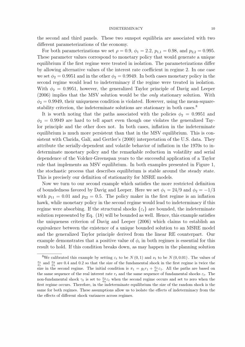
INDETERMINACY 10

the second and third panels. These two sunspot equilibria are associated with twodifferent parameterizations of the economy.

For both parameterizations we set ρ = 0.9, φ1 = 2.2, p1,1 = 0.98, and p2,2 = 0.995.These parameter values correspond to monetary policy that would generate a uniqueequilibrium if the first regime were treated in isolation. The parameterizations differby allowing alternative values of the interest rate coefficient in regime 2. In one casewe set φ2 = 0.9951 and in the other φ2 = 0.9949. In both cases monetary policy in thesecond regime would lead to indeterminacy if the regime were treated in isolation.With φ2 = 0.9951, however, the generalized Taylor principle of Davig and Leeper(2006) implies that the MSV solution would be the only stationary solution. Withφ2 = 0.9949, their uniqueness condition is violated. However, using the mean-square-stability criterion, the indeterminate solutions are stationary in both cases.8

It is worth noting that the paths associated with the policies φ2 = 0.9951 andφ2 = 0.9949 are hard to tell apart even though one violates the generalized Tay-lor principle and the other does not. In both cases, inflation in the indeterminateequilibrium is much more persistent than that in the MSV equilibrium. This is con-sistent with Clarida, Galí, and Gertler’s (2000) interpretation of the U.S. data. Theyattribute the serially-dependent and volatile behavior of inflation in the 1970s to in-determinate monetary policy and the remarkable reduction in volatility and serialdependence of the Volcker-Greenspan years to the successful application of a Taylorrule that implements an MSV equilibrium. In both examples presented in Figure 1,the stochastic process that describes equilibrium is stable around the steady state.This is precisely our definition of stationarity for MSRE models.

Now we turn to our second example which satisfies the more restricted definitionof boundedness favored by Davig and Leeper. Here we set φ1 = 24/9 and φ2 = −1/3

with p11 = 0.01 and p22 = 0.5. The policy maker in the first regime is an inflationhawk, while monetary policy in the second regime would lead to indeterminacy if thisregime were absorbing. If the structural shocks {εt} are bounded, the indeterminatesolution represented by Eq. (18) will be bounded as well. Hence, this example satisfiesthe uniqueness criterion of Davig and Leeper (2006) which claims to establish anequivalence between the existence of a unique bounded solution to an MSRE modeland the generalized Taylor principle derived from the linear RE counterpart. Ourexample demonstrates that a positive value of φi in both regimes is essential for thisresult to hold. If this condition breaks down, as may happen in the planning solution

8We calibrated this example by setting εt to be N (0, 1) and νt to be N (0, 0.01) . The values ofκ1φ1

and κ2φ2

are 0.4 and 0.2 so that the size of the fundamental shock in the first regime is twice thesize in the second regime. The initial condition is π1 = g1r1 + κ1

φ1ε1. All the paths are based on

the same sequence of the real interest rate rt and the same sequence of fundamental shocks εt. Thenon-fundamental shock γt is set to κ2

φ2εt when the second regime occurs and set to zero when the

first regime occurs. Therefore, in the indeterminate equilibrium the size of the random shock is thesame for both regimes. These assumptions allow us to isolate the effects of indeterminacy from thethe effects of different shock variances across regimes.

INDETERMINACY 11

discussed by Rotemberg and Woodford (1999a, Page 83), there will exist sunspotequilibria in general whenever there is a sunspot equilibrium in at least one regimeconsidered in isolation. This example raises serious questions about the validity ofthe generalized Taylor principle for MSRE models.

VIII. Conclusion

We have shown in this paper that the distinction between linear and MSRE modelsis important but its consequences for equilibrium are not well understood. We havedemonstrated that the properties of uniqueness, stationarity and boundedness, evenfor the simple MSRE model of monetary policy studied in this paper, are fundamen-tally different from those of linear models. Characterizing the full class of equilibriaremains a challenging task. Contrary to the existing literature, we have shown thatmultiple equilibria are more prevalent than commonly thought and that the dynamicbehavior of equilibrium sample paths depends in subtle ways on both the current andthe past realized regimes. Regrettably, the generalized Taylor principle does not holduniversally, even for a simple MSRE model.

INDETERMINACY 12

Appendix A. Proof of Proposition 3

Substituting Eq. (7) into Eq. (8) we have,

πt = gξtrt +1

φξt

Et[πt+1 − gξt+1rt+1] +κξt

φεt

εt.

Substituting for rt+1 from (4) and collecting terms leads to

πt =1

φξt

Et[πt+1] +1

φξt

rt[φξtgξt − ρ(p1,ξtg1 + p2,ξtg2)] +κξt

φξt

εt.

or sincep1,ξtg1 + p2,ξtg2 ≡ Etgξt+1

πt =1

φξt

Et[πt+1] +1

φξt

rt[φξtgξt − ρEtgξt+1 ] +κξt

φξt

εt,

Note that if ξt = 1, it follows from (5) that

(φ1 − ρp1,1)g1 − ρp2,1g2 = 1.

Similarly, if ξt = 2, it follows from (5) that

−ρp1,2g1 + (φ2 − ρp2,2)g2 = 1.

Hence we haveπt =

1

φξt

Et [πt+1] +1

φξt

rt +κξt

φξt

κξtεt,

which is equivalent to (3).

Appendix B. Proof of Proposition 4

We first show that ηt+1 has zero conditional mean. If ξt = 1,

Et [ηt+1] = p1,1κ1

φ1

Et [εt+1] + p2,1

(Et [γt+1] +

κ2

φ2

Et [εt+1]

)= 0,

and if ξt = 2,

Et [ηt+1] = p1,2

(κ1

φ1

Et [εt+1]− 1

a2

(xt − κ2

φ2

εt

))

+ p2,2

(Et [γt+1] +

κ2

φ2

Et [εt+1] + φ2p1,2

p2,2

(xt − κ2

φ2

εt

))= 0.

Next, we derive the solution to Eq. (8). Given x1, the sequence {xt+1}∞t=1 can beconstructed recursively from the following transition equations, which are derived byusing Eq. (9) and Definition (15). When ξt = 1,

xt+1 =

1a1

(xt − κ1

φ1εt

)+ κ1

φ κξtφεt

εt+1, if ξt+1 = 1,

1a1

(xt − κ1

φ1εt

)+ γt+1 + κ2

φ2εt+1, if ξt+1 = 2;

(A1)

INDETERMINACY 13

and when ξt = 2,

xt+1 =

{κ1

φ1εt+1, if ξt+1 = 1,

φ2

(xt − κ2

φ2εt

)+ γt+1 + κ2

φ2εt+1 + φ2

p1,2

p2,2(xt − σ2εt) , if ξt+1 = 2.

(A2)

Since we have imposed the initial condition x1 = κ1

φ1ε1, it follows by induction from

Eqs. (A1) and (A2) that when ξt+1 = 1, xt+1 = κ1

φ1εt+1 for all t ≥ 1. The transition

from state 1 to state 2 can be simplified using this initial condition, and Eq. (A1)can be written as the expression (16). Eq. (A2) can be also simplified, using the factthat p1,2 + p2,2 = 1, to yield the expression (17). The initial condition (14) and Eqs.(16) and (17) completely characterize the evolution of xt for t = 1, ...∞.

Finally, we show that lims→∞ Et [xt+s] = 0. Using Eqs. (16) and (17), we obtainthe following expression:

Et [xt+1] =

{0, if ξt = 1,

φ2

(xt − κ2

φ2εt

), if ξt = 2.

A simple induction argument, again using Eqs. (16) and (17) shows that,

Et [xt+s] = Et [Et+1 [xt+k]] =

{0, if ξt = 2,

(φ2)s(xt − κ2

φ2εt

), if ξt = 2.

Because |φ2| < 1, lims→∞ Et [xt+s] = 0. Since {γt+1} is arbitrary, we have completedthe proof that {{ηt+1}∞t=1 , x1} generates multiple solutions.

Appendix C. Proof of Proposition 5

Theorem 3.33 of Costa, Fragoso, and Marques (2004) implies that, if the Markovchain is ergodic, we need only show that solutions given by (14), (16), and (17) aremean-square stable when εt and γt are zero. By Theorem 3.9 of CFM, the stabilitycondition is equivalent to showing that there exist constants 1 ≤ β < ∞ and 0 < ζ < 1

such thatE1

[x2

t

] ≤ βζt−1x21,

for t ≥ 1. When εt and γt are zero, xt will be non-zero only if ξ1 = · · · = ξt = 2. In

this case, xt =(

1a2p2,2

)t−1

x1 and this event occurs with probability pt−12,2 . Thus

E1

[x2

t

]= pt−1

2,2

(φ2

p2,2

)2(t−1)

x21,

=

(φ2√p2,2

)2t−2

x21.

The results now follow from the assumption that∣∣∣ φ2√

p2,2

∣∣∣ < 1.

INDETERMINACY 14

References

Clarida, R., J. Galí, and M. Gertler (2000): “Monetary Policy Rules and MacroeconomicStability: Evidence and Some Theory,” Quarterly Journal of Economics, 115(1), 147–180.Costa, O., M. Fragoso, and R. Marques (2004): Discrete-Time Markov Jump Linear Systems.Springer, New York.Davig, T., and E. Leeper (2005): “Generalizing the Taylor Principle,” NBER Working Paper11874.

(2006): “Generalizing the Taylor Principle,” Mimeo: University of Indiana.Farmer, R. E. A., D. F. Waggoner, and T. Zha (2006): “Minimal State Variable Solutions toMarkov-Switching Rational Expectations Models,” UCLA mimeo.Hamilton, J. D. (1994): Times series analsis. Princeton University Press, Princeton, NJ.King, R. G. (2000): “The New IS-LM Model: Language, Logic, and Limits,” Federal Reserve Bankof Richmond Economic Quarterly, 86/3, 45–103.Rotemberg, J., and M. Woodford (1999a): Monetary Policy Ruleschap. 2, pp. 57–126. NBER.Rotemberg, J. J., and M. Woodford (1999b): “Interest Rate Rules in an Estimated StickyPrice Model,” in Monetary Policy Rules, ed. by J. B. Taylor, pp. 57–119. University of ChicagoPress, Chicago.Sims, C. A. (2001): “Solving Linear Rational Expectations Models,” Journal of ComputationalEconomics, 20(1-2), 1–20.Svensson, L., and N. Williams (2005): “Monetary Policy with Model Uncertainty: DistributionForecast Targeting,” Princeton University Mimeo.Woodford, M. (2003): Interest and Prices: Foundations of a Theory of Monetary Policy. Prince-ton University Press, Princeton, N.J.