region-wide wastewater treatment plant modeling enhances...

Region-wide Wastewater Treatment Plant Modeling Enhances Facility Management and Planning

Christopher M. Bye1*, José R. Bicudo2, Richard M. Jones1

1 EnviroSim Associates Ltd., Hamilton, Ontario, Canada 2 Regional Municipality of Waterloo, 150 Frederick Street, Kitchener, Ontario, Canada * Email: [email protected].

ABSTRACT

This paper shows the results of linking several regional WWTPs in a model-based analysis. The Galt wastewater treatment plant was used as a case study to show how decisions made at one plant can impact the future plans for other plants. This approach facilitates planning on a region-wide basis, helps decision makers maximize the capacity of existing treatment plant infrastructure, allows for the sharing (where possible) of excess WWTP capacity, achieves maximum benefit from new infrastructure, provides a basis for more detailed work related to individual unit process optimization (e.g. collection of additional data around individual unit processes, stress testing, etc.), and aids in the development of rational plant upgrade strategies to accommodate future growth.

KEYWORDS: modeling, planning, plant management.

INTRODUCTION

Wastewater treatment plant process modeling is a powerful tool that can help decision makers maximize the capacity of existing treatment plant infrastructure, achieve maximum benefit from new infrastructure, and aid in the development of capital improvement programs (CIPs) to accommodate future growth.

Although many treatment plant owners have used process modeling for macro-level, multi-plant Master Plan-level applications, as well as detailed analysis of single, stand-alone wastewater treatment plants, to date there have been few applications that examine potential interactions between several treatment plants through model-based analysis. The results of such an analysis can provide owners that are responsible for several plants across a geographical region with information that can be used to facilitate planning on a region-wide basis. An example of this type of analysis will be given via explanation of a project completed by EnviroSim Associates Ltd. and the Regional Municipality of Waterloo (Ontario, Canada) using the BioWin wastewater treatment process model.

BACKGROUND ON THE REGIONAL MUNICIPALITY OF WATERLOO

The Regional Municipality of Waterloo is responsible for overseeing the treatment of wastewater generated by the Cities of Kitchener, Waterloo and Cambridge and the Townships of North

8339

WEFTEC 2012

Copyright ©2012 Water Environment Federation. All Rights Reserved.

Dumfries, Wellesley, Wilmot and Woolwich; several pumping stations; the Wellesley and North Dumfries collection systems and the management of biosolids generated at its facilities.

The Region operates 13 wastewater treatment plants (WWTPs) through a contractor. The plants provide a minimum of secondary treatment for approximately 180 MLD (47.6 mgd) of wastewater. Treatment capacities for the individual plants vary from 0.13 MLD (0.03 mgd) to 122.7 MLD (32.4 mgd). The Region’s 2011 Ten-Year Wastewater Capital Program provides a total budget of $717 million. Over 70% of the 10-year wastewater capital upgrades and expansion budget is allocated for work at three WWTPs in Kitchener, Waterloo and Hespeler. In general, the upgrades to these facilities will improve effluent water quality in the Grand River, replace aging equipment, improve process efficiency, mitigate odours and provide biosolids dewatering at the Kitchener and Waterloo WWTPs. The Region and/or their consultants use WWTP modeling as a tool for a variety of engineering applications, including Master Plans, plant capacity estimation, design, and operation scenario investigations.

INTERACTIONS BETWEEN GALT, PRESTON, AND OTHER WWTPS

Models have been formulated for several Region WWTPs. Potential interactions between two of the larger plants [Galt (56.8 MLD, 15 mgd); Preston (16.86 MLD, 4.5 mgd)] were examined in a recently completed project. The findings from these studies have allowed better plant operation decisions, infrastructure spending planning, and plant upgrade strategies.

Upgrades to the Galt WWTP solids treatment train have been completed, including refurbishment of anaerobic digesters and construction of a biosolids dewatering facility with mechanical thickening and dewatering equipment. A calibrated model-based scenario analysis was performed to investigate:

1. The Galt WWTP performance after completion of the proposed upgrades; 2. The feasibility of the Galt WWTP dewatering digested biosolids from other WWTPs

following the recommendations of the appropriate Class EA study completed in 2008; 3. The feasibility of diverting part or all of the wastewater flow from the Industrial Road

Service Area (IRSA) from the Preston WWTP to the Galt WWTP following the recommendations of the Wastewater Treatment Master Plan completed in 2007.

STRUCTURED APPROACH FOR MODEL APPLICATION

The suggested steps for applying a wastewater treatment process model to estimate plant capacity, assess optimal use of new plant infrastructure, etc. are listed below. Details and further discussion are provided for each.

Step 1 – Configure and Calibrate Plant Model Configuring and calibrating a wastewater treatment plant model requires information in the following general categories as input data for the simulator:

8340

WEFTEC 2012


1. Plant physical data: This relates to the size of units in the treatment system. For example, aeration tank dimensions (volume, length, width and depth), clarifier area and depths, and so on.

2. Plant operating data: This includes data on operational aspects such as primary sludge flow rates, return activated sludge (RAS) flow rates, wastage activated sludge (WAS) flow rates, mixed liquor recycle flows, and DO concentrations in aerated zones, air flow rates, etc.

3. Influent loading data: The influent flow and concentrations obviously are essential data. This refers to raw influent wastewater (a) flow rate data, and (b) concentrations of a range of parameters (COD or BOD, VSS, TSS, TKN, NH3-N, TP, PO4-P, Alkalinity, pH, etc.). Depending on the overall project objectives, diurnal variability of flow and composition may be important, as well as unusual events such as storm flows.

4. Influent wastewater characteristics: An important part of the influent data is the wastewater characterization; that is, the division of bulk concentration measures such as total COD into various characteristic sub-portions. Typically, it is not possible to derive these from routinely collected plant data. To address this, a supplemental sampling program may be carried out at the plant to collect the data necessary for estimating the characteristic fractions.

5. Kinetic and/or stoichiometric model parameters: Experience shows that these parameters should not change appreciably from plant to plant unless there are special circumstances such as industrial inputs and/or the influent contains components that inhibit the biological process (e.g. incinerator scrubber water containing cyanide). The one exception to this rule possibly is the nitrifier maximum specific growth rate, which can have a significant impact on plant capacity. As such, it often is prudent to measure this parameter.

Once the information listed above has been gathered, the simulator is ready to be calibrated. A rigorous approach for model calibration involves running long-term dynamic simulations (e.g. one year period) of a historical dataset representing stable plant operation. A Water Environment Research Foundation manual provides a comprehensive overview of model calibration (WERF, 2003).

A common misconception is that calibrating a model only involves matching the model predictions for effluent quality to observed data. For example, concentrations of significant parameters in the secondary effluent (e.g. COD, TSS, NH3-N, NO3-N, PO4-P, Alkalinity, pH). While this is undoubtedly important, a calibrated model should also provide reasonable predictions for a wide range of plant performance characteristics. These include data such as:

• Primary effluent quality (if the plant has primary clarifiers): This refers to primary effluent (a) flow rate data, and (b) concentrations of a range of parameters (COD, BOD, VSS, TSS, TKN, NH3-N, TP, PO4-P, etc.).

• Return stream quality: This refers to concentrations of significant parameters in plant return/recycle streams such as anaerobic digester supernatant (e.g. COD, TSS, NH3-N, NO3-N, PO4-P, Alkalinity, pH).

8341

WEFTEC 2012


• In-process solids concentrations: This includes mixed liquor VSS and TSS, secondary clarifier underflow VSS and TSS.

• Sludge production: Primary and WAS sludge VSS and TSS mass rates and final dewatered sludge mass.

It should be noted that often it is not possible to adjust simulator parameters such that an exact match between predicted and observed values is achieved. It is preferable to fit to most of the measured variables reasonably, rather than fit perfectly to one selected (albeit perhaps important) component concentration and poorly to others. It is important that the calibrated model achieves a good correlation between the overall trend of predicted and observed values while minimizing the error between datasets and simulator predictions.

Step 2 – Identify Constraints for Modelling Scenarios Once the model has been calibrated, the next step is to identify any constraints that should be recognized for the modelling scenarios. Examples could include:

• Equipment constraints: These should be incorporated into the model and may include plant aspects such as blower capacities, RAS pump limits, potential units out of service, etc.

• Operating constraints: These often form the “rules” that need to be kept in mind when applying the model and may include minimum solids retention time for nitrification (if applicable), maximum allowable mixed liquor concentrations, anaerobic digester hydraulic retention time, dewatering facility operating shift lengths, etc.

Step 3 – Establish Key Performance Indicators (KPIs) This step involves selecting which parameters should be tracked when simulating scenarios; that is, the KPIs. These may be thought of as the model outputs that are of the most relevance. Usually the focus is on ensuring that plant effluent limits are met. However other related operational items also are often of importance, such as secondary clarifier solids loading rate, aeration tank dissolved oxygen fluctuations, etc.

Step 4 – Establish Modelling Scenarios Once constraints and KPIs have been established, the next step is to define scenarios to be modelled. Often this consists of identifying temperature, flow and load patterns to apply in conjunction with estimated future daily average flows. It also may involve testing whether or not the plant can accept an additional input such as hauled septage, an industrial flow diversion or biosolids from other nearby plants.

Step 5 – Run Modelling Scenarios Once the model has been calibrated, constraints have been identified, KPIs have been established, and the modelling scenarios of interest have been identified, it is time to run the scenarios in the model. In evaluating the simulation results, the KPIs should be examined relative to the established constraints and targets. It may be necessary to run modelling scenarios iteratively, particularly if the objective is to determine the ultimate plant capacity with existing infrastructure.

8342

WEFTEC 2012


APPLYING THE STRUCTURED APPROACH FOR GALT WWTP

The Galt WWTP is owned by the Region of Waterloo (ROW) and operated by the Ontario Clean Water Agency (OCWA). The facility provides tertiary treatment with activated sludge incorporating nitrification, chemical phosphorus removal, and sludge processing. Liquid treatment consists of mechanical screening, grit removal, primary clarifiers, biological reactors incorporating fine pore diffused aeration, secondary clarifiers, single-media automatic backwash effluent filters, and ultraviolet disinfection with sodium hypochlorite backup. The solids treatment train for handling primary sludge and waste activated sludge (WAS) currently includes two primary digesters, one sludge holding tank, and a digester gas handling/utilization system. When the project commenced, the plant was operated in a co-thickening mode, where WAS generated in the biological reactors was directed to the primary clarifiers (this practice has been stopped after completion of upgrades). In addition, primary sludge and WAS were processed by one primary digester followed by one secondary digester. The existing plant has a Stage 1 nominal rated capacity of 56,800 m3/d (15 mgd).

Upgrades to the solids treatment train have now been completed. Primary digestion facility upgrades include new raw sludge pumps, a new primary digester roof equipped with roof-mounted vertical-flow draft tubes with shaft-mounted propeller mixers, and a sludge heating/recirculation system. A new biosolids management facility includes rotary drum thickeners for WAS thickening (which ended the previous practice of co-thickening), thickened WAS pumps, a digested sludge holding tank, centrifuges for digested sludge dewatering, and a centrate/filtrate holding tank. More recently, the secondary digester was converted to a primary digester with the two digesters currently operating in series. A calibrated model-based scenario analysis was performed to investigate:

1. The Galt WWTP performance after completion of the proposed upgrades; 2. The feasibility of the Galt WWTP dewatering digested biosolids from other WWTPs

following the recommendations of the appropriate Class EA study completed in 2008; 3. The feasibility of diverting part or all of the wastewater flow from the Industrial Road

Service Area (IRSA) from the Preston WWTP to the Galt WWTP following the recommendations of the Wastewater Treatment Master Plan completed in 2007.

Various combinations of these scenarios were investigated for current and estimated future Galt WWTP raw influent flows.

Step 1 – Galt Model Calibration A model was configured for the Galt WWTP and calibrated to historical data from the March 2007 – February 2008 period. Figure 1 shows the pre-upgrade Galt WWTP represented in BioWin™.

8343

WEFTEC 2012


Figure 1: Overall model layout for the Galt treatment plant.

Before commencing the model calibration, the plant data for the one year calibration period were reviewed. The data were assembled in one master spreadsheet for the entire period to facilitate transfer into the BioWin wastewater treatment process simulator. The calculation of ratios between some of these influent characteristics and comparison to typical values is of particular importance at this stage. Table 1 summarizes the statistics calculated for the raw influent data. The following points were observed:

• The average TSS/BOD ratio was higher than the typical range. Cross-checks with other ratios indicated that this ratio is high because the average TSS concentration is high given the organic strength of the wastewater. There are no COD or VSS data in the historical dataset to serve as a cross-check, however the supplemental sampling data indicated that the reason for the high solids is a higher than typical particulate unbiodegradable COD portion in the influent.

• The average TKN/BOD ratio was within the typical range.

• The average TP/BOD ratio was within the typical range. Table 1: Statistics calculated for raw influent parameters and selected ratios for period March 1, 2007 to February 29, 2008.

Parameter Average Typical Range Flow (m3/d) 36,941 BOD (mg/L) 199 TSS (mg/L) 249 TKN (mg/L) 37.2 TP (mg/L) 4.8 TSS/BOD 1.39 0.70 – 1.22 TKN/BOD 0.19 0.14 – 0.24 TP/BOD 0.02 0.02 – 0.05

8344

WEFTEC 2012


As a result of the plant data review, additional data requirements were identified and a supplemental sampling plan was formulated and executed by EnviroSim staff over two weeks during February 2008. Grab samples were collected daily at the same time for a number of streams, including raw influent, primary effluent, secondary effluent, mixed liquor, return activated sludge (RAS), and primary sludge. Wastewater characteristics derived from this exercise are listed in Table 2 below. Many of these values fall within ranges typically observed at North American wastewater treatment plants, with the exception of the following:

• The fraction of influent TKN in the form of ammonia (FNA) is lower than typical.

• The fraction of influent TKN that is unbiodegradable and soluble (FNUS) is higher than typical. It is suspected that this may be a transient phenomenon, possibly due to periodic discharges from textile industries in the area, as there was not evidence of excess unbiodegradable soluble nitrogen on each day it was tested for. Note that testing for FNUS was not in the original sampling plan because an effluent TN limit is not anticipated at this plant. However, ongoing data evaluation during the initial stages of the sampling campaign indicated high influent organic nitrogen content. Therefore, the effluent soluble organic nitrogen concentration was checked to ascertain the nature of this material. The unbiodegradable soluble nitrogen in the influent is likely the cause of the lower than typical FNA. Other checks (e.g. the influent TKN/COD ratio) indicate that the influent total nitrogen content is high relative to the organic strength.

• The fraction of the influent COD that is unbiodegradable particulate (FUP) is on the high end of the typical range (WERF, 2003). This parameter cannot be measured directly; rather it must be inferred from a combination of other ratios including COD:BOD, COD:VSS, and TSS:BOD. Analysis of the supplemental sampling data indicated a higher than typical FUP fraction, and this was corroborated by examination of the historical dataset. The implication of using a higher than typical FUP in the calibrated model for scenario analysis is that model will tend to be conservative in terms of sludge production predictions.

Table 2: Wastewater fractions and ratios derived from supplemental sampling for use in model calibration.

Constituent Fraction Value

Fbs - Readily biodegradable (including Acetate) [gCOD/g of total COD] 0.19

Fxsp - Non-colloidal slowly biodegradable [gCOD/g of slowly degradable COD] 0.85

Fus - Unbiodegradable soluble [gCOD/g of total COD] 0.05

Fup - Unbiodegradable particulate [gCOD/g of total COD] 0.22

Fna - Ammonia [gNH3-N/gTKN] 0.43

Fnus - Soluble unbiodegradable TKN [gN/gTKN] 0.09

Fpo4 - Phosphate [gPO4-P/gTP] 0.50

Fcvxi, Fcvxs - Particulate biodegradable and unbiodegradable COD:VSS ratio [gCOD/gVSS] 1.7

8345

WEFTEC 2012


The model was calibrated to a variety of plant parameters, including mixed liquor suspended solids levels, as shown in Figure 2.

Figure 2: Predicted (line) versus observed (points) train #1 (top) and train #2 (bottom) aeration tank MLSS.

Due to instrumentation issues, it only was possible to obtain instantaneous airflow readings from the plant SCADA interface (DO readings were not logged to the SCADA database). Given the intended application of the calibrated model, EnviroSim attempted to gain further insight to the aeration system at the Galt WWTP (and hence add further rigour to the model) through the following exercise.

On November 17th, 2008 EnviroSim measured DO concentrations in the train #2 aeration tank at the influent end of the first pass and the mid-point of the second pass (the DO probe was calibrated in situ). The initial readings obtained within a few minutes of each other are shown in Table 3. Table 3: Train #2 aeration tank DO spot-checks obtained on November 17th, 2008.

Reading Number

Aeration Tank DO At Influent End of First Pass (mg/L)

Aeration Tank DO At Mid-Point of Second Pass (mg/L)

1 4.50 6.03 2 4.96 6.07 3 4.85 5.75

These readings were obtained with an airflow of approximately 1,800 L/s directed to the train #2 aeration tank (observed from the SCADA interface). At this time, two of the plant’s four available blowers were operating in a partially throttled mode such that they were delivering approximately 70% of their capacity.

MLSSMLSS (obs)

Galt WWTP Mixed Liquor Train #1

Feb-08Jan-08Dec-07Nov-07Oct-07Sep-07Aug-07Jul-07Jun-07May-07Apr-07Mar-07

CO

NC

(mg/

L)

5,000

4,000

3,000

2,000

1,000

0

MLSSMLSS (obs)

Galt WWTP Mixed Liquor Train #2

Feb-08Jan-08Dec-07Nov-07Oct-07Sep-07Aug-07Jul-07Jun-07May-07Apr-07Mar-07

CO

NC

(mg/

L)

5,000

4,000

3,000

2,000

1,000

0

8346

WEFTEC 2012


While these spot-checks indicate that DO was not limiting at that time, a further check was conducted by obtaining DO concentrations over a longer period. EnviroSim has developed a DO controller that is used for experimental studies (e.g. wastewater characterization SBRs, High F/M tests). This instrument also can be used as a standard DO meter. One useful feature is the ability to log DO measurements at a pre-set interval to a USB memory stick. A photo of this unit is shown below:

Figure 3: DO controller / meter developed and manufactured by EnviroSim.

The DO probe was mounted to a boom located at the influent end of the first aeration tank pass. The instrument was set up to log DO concentration readings every ten seconds. The DO logging commenced at approximately 11:50 am on November 17th, 2008 and ceased about eighteen hours later (the portable generator used to supply power to the unit ran out of fuel at this time). The DO measurements recorded over this time period are shown in Figure 4 below:

8347

WEFTEC 2012


Figure 4: Dissolved concentration observed at the influent end of the West aeration tank first pass over 18 hours (November 17th-18th, 2008).

The DO data recorded during this exercise suggest that blower capacity should not be a limiting factor at the Galt WWTP.

In an effort to translate these findings to the Galt WWTP plant model, simulations were performed to investigate whether the model could predict the DO/airflow interaction observed in the train #2 aeration tank. Airflow values were input to the model and a one day simulation (using the actual influent flow data from that day) was run to investigate whether the DO response could be adequately simulated using a total airflow value approximating the value observed on the SCADA screen. Figures 5 and 6 below show that the DO response in the first pass could be accurately simulated, and the model prediction for the total airflow required also agreed with the approximate values obtained from the SCADA system for that day.

Figure 5: Input airflow (total and individual zones) compared to estimate obtained from SCADA (red dotted line).

0

1

2

3

4

5

6

7

8

11:31:12 AM 1:55:12 PM 4:19:12 PM 6:43:12 PM 9:07:12 PM 11:31:12 PM 1:55:12 AM 4:19:12 AM

DISSOLVED

OXY

GEN CONCE

NTR

ATION (m

g/L)

TIME

Pass 1Pass 2Pass 3Aeration Tank Total

Galt WWTP Aeration Tank Air Supply Rate

11 18 10:0011 18 8:0011 18 6:0011 18 4:0011 18 2:0011 18 0:0011 17 22:0011 17 20:0011 17 18:0011 17 16:0011 17 14:0011 17 12:00

AIR

FLO

W (m

3/h)

20,000

15,000

10,000

5,000

0

8348

WEFTEC 2012


Figure 6: Predicted versus observed train #2 aeration tank dissolved oxygen.

At this stage, the influent the Galt WWTP was considered well-characterized and the BioWin model of the plant was considered to be calibrated to a degree that it could be applied to scenario analysis with confidence.

Step 2 –Constraints for Galt Modelling Scenarios The calibrated model was modified to account for the completed (at that time) upgrades to the plant solids handling train. Modifications included waste activated sludge (WAS) thickening (i.e. the cessation of co-thickening of WAS in the primary settling tanks [PSTs]), incorporation of a digested sludge holding tank, addition of centrifuges, and a centrate holding tank. Incorporating these changes resulted in additional loading to the plant principally in the form of returned centrate. Additional inputs to the model to represent diverted industrial flow from the Industrial Road Service Area (IRSA) and biosolids from other Region plants were included. The modified model flowsheet used for scenario analysis is shown in Figure 7.

Figure 7: Model process flowsheet used for scenario analysis.

Cell 2-1 (obs)Cell 2-1Cell 2-2Cell 2-3

Galt WWTP Dissolved Oxygen

11 18 10:0011 18 8:0011 18 6:0011 18 4:0011 18 2:0011 18 0:0011 17 22:0011 17 20:0011 17 18:0011 17 16:0011 17 14:0011 17 12:00

CO

NC

(mg/

L)8

7

6

5

4

3

2

1

0

8349

WEFTEC 2012


Important equipment and operational constraints incorporated into the Galt scenario modelling included information about the plant nitrifier maximum specific growth rate, the operating SRT required to maintain nitrification at winter temperatures, air supply capacity, RAS pumping limits, thickening factors achievable in the solids handling train unit processes, and the length of solids handling equipment shift runs. Key constraints are summarized in Table 4 below.

Table 4: Key assumptions underlying model-based scenario analysis.

Assumption Comments

Nitrifier growth rate of 0.85 d-1 The BioWin default value for this parameter is 0.90 d-1, and this value was used in the model calibration exercise with good results. Commonly measured values in North America range from 0.8-1.0 d-1 (WERF, 2003). A value of 0.85 d-1 was selected for the scenario analysis because that was the value measured by EnviroSim at a nearby Region WWTP, and it introduces a degree of conservatism to the analysis.

Operating SRT of 7.5 days At the time of the study the plant was operated at an average SRT in the region of 9 days. Based on the nitrifier growth rate assumption discussed above, it appears that the plant can achieve nitrification at winter conditions at a lower SRT. The lower SRT helps to keep MLSS levels reasonable at higher future loadings.

PST Solids Capture A solids capture rate of 65% was used for the model calibration. This capture rate was assumed to prevail for future flow scenarios.

Aeration tank dissolved oxygen (DO) levels of 2 mg/L achievable.

As documented in the model calibration phase, under current loading conditions with two blowers running at 70% of capacity the DO at the front end of the first pass of the West aeration tank was at or above 4 mg/L for most of a typical day. It appears as though the aeration equipment at the Galt WWTP should be able to achieve aeration tank DO levels of 2 mg/L at the future flows and loads under consideration.

Return activated sludge (RAS) The plant is operated with the RAS rates for the final settling tanks set to approximately 100% of the average flow treated in each train. This practice has been maintained for future flow scenarios.

8350

WEFTEC 2012


Table 4, cont’d

Thickening Factors1 The concentration of certain plant solids streams are determined as a result of the degree of thickening achieved in various unit processes (e.g. primary sludge, WAS) and these have been set in the analysis according to design guidelines or actual data observed at the Galt WWTP as follows: o Primary sludge was assumed to achieve a

concentration of approximately 3.3%, based on measurements conducted by EnviroSim during the supplemental sampling campaign in February 2008.

o Thickened WAS was assumed to achieve a concentration of approximately 7%, based on typical design guidelines (Metcalf & Eddy, 2003).

o Dewatered sludge was assumed to achieve a concentration of approximately 20%, based on typical design guidelines (Metcalf & Eddy, 2003).

Temperature All scenarios were conducted at a temperature of 12 °C

Wastewater characteristics obtained from the supplemental sampling exercise conducted (February, 2008) in support of the Galt WWTP model calibration were assumed to hold for future flow conditions. Concentrations for various bulk parameters (e.g. COD, TSS) were assumed to remain at values representative of those observed over the 2007-2008 period; that is, overall mass loading on the plant is assumed to increase as a result of increasing raw influent flow.

A daily raw influent flow pattern is desirable for conducting dynamic simulation analysis. During visits to the Galt WWTP, EnviroSim obtained printouts of hourly flow records over 24-hour periods. These were not readily available in electronic form, which would have allowed for a more rigorous analysis of historical flow data using an EnviroSim-developed flow analysis tool. However, a typical flow day (November 17th, 2008) when there was no significant storm or snow-melt influx to the collection system was selected and normalized to establish the pattern shown in Figure 8 below.

1 Because the model obeys a mass balance, the concentration of thickened streams determines their “flows”. In the case of the primary sludge and thickened WAS streams, the flow is important in that it determines the primary digester hydraulic retention time (HRT).

8351

WEFTEC 2012


Figure 8: Normalized daily flow pattern used as a basis for scenario analysis (Peak:Mean Ratio – 1.25, Min:Mean Ratio – 0.63).

Projected future flows obtained from the Region are listed in Table 5 below. These are plotted versus time in Figure 9; there generally is a linear increase in plant raw influent flows with time.

Table 5: Projected raw wastewater flows to the Galt WWTP.

Year Projected Flow (m3/d)

2021 45,900

2031 51,100

2041 54,400

0.0

0.2

0.4

0.6

0.8

1.0

1.2

1.4

0 4 8 12 16 20 24

NO

RM

ALIZ

ED F

LOW

...

TIME (HRS)

8352

WEFTEC 2012


Figure 9: Raw influent flow projections for the Galt WWTP.

To provide a daily raw influent flow pattern for a given scenario year, the normalized daily flow pattern from Figure 8 was multiplied by the average flow value for that year from Table 5. Raw influent concentrations were assumed to remain constant throughout the day, which means that the raw influent daily mass loading pattern for wastewater constituents such as BOD, etc. tracks the daily flow pattern. This is a conservative assumption, since typically plant daily mass loading patterns do not exhibit as much variability as daily flow patterns.

The Region commissioned a sampling campaign of the IRSA wastewater to obtain more detailed information on the concentration of various constituents. Given the large food processing component of this wastewater, it is quite high in organic strength and suspended solids. However, it is not strong in terms of nitrogen or phosphorus. Daily and overall average concentrations are shown in Table 6. Based on this information, it was possible to derive the wastewater characteristic fractions shown in Table 7.

y = 1.284x -‐ 11119R² = 0.9888

0

10000

20000

30000

40000

50000

60000

01/01/2010 30/12/2019 27/12/2029 25/12/2039

FLOW (m

3 /d)

DATE

8353

WEFTEC 2012


Table 6: IRSA data collected during Region of Waterloo sampling campaign and used as model inputs.

Table 7: Wastewater fractions derived from IRSA supplemental sampling.

Constituent Fraction Value

Fbs - Readily biodegradable (including Acetate) [gCOD/g of total COD] 0.25

Fxsp - Non-colloidal slowly biodegradable [gCOD/g of slowly degradable COD] 0.70

Fus - Unbiodegradable soluble [gCOD/g of total COD] 0.00

Fup - Unbiodegradable particulate [gCOD/g of total COD] 0.13

Fna - Ammonia [gNH3-N/gTKN] 0.12

As was the case for the raw influent flow, a daily IRSA flow pattern was desirable. The Region had extensive flow data collected over two periods (several months in the Spring of 2008, and during the IRSA supplemental sampling in October 2008). The data consisted of flow rates recorded every 10 minutes. Because these data were available in electronic form, EnviroSim was able to conduct a rigorous analysis of the data using an EnviroSim-developed flow analysis tool. Essentially this tool rapidly scans through the data and extracts daily 24-hour flow patterns for each day of the week contained in the dataset. The tool allows for screening of each day’s flow patterns (e.g. days with large gaps in the flow records were removed), and then calculates the average daily flow pattern for each day of the week, as shown in Figure 10 below.

TSS VSS COD COD BOD cBOD TP ALK pH Ca Mg TKN NH3-NDATE DAY tot. 1.5µ gf tot. tot.

(mg/L) (mg/L) (mg/L) (mg/L) (mg/L) (mg/L) (mg/L) (mgCaCO3/L) (mg/L) (mg/L) (mg/L) (mg/L)

2008-10-15 0 1410 3130 1150 1240 1090 2.9 456 130.0 33.8 119.0 17.32008-10-16 1 1230 4080 1150 1640 1520 6.0 471 6.4 182.0 32.1 111.0 17.22008-10-18 2 884 1180 1320 941 13.8 437 6.5 168.0 37.5 145.0 25.32008-10-19 3 566 1350 390 1170 1100 5.2 351 6.5 162.0 29.4 68.9 4.52008-10-20 4 1360 960 3230 2250 1540 6.8 290 5.9 248.0 39.9 111.0 3.62008-10-23 5 480 480 2100 1060 1380 1310 4.9 434 6.6 172.0 39.3 113.0 17.02008-10-24 6 402 440 1950 1110 1330 1430 4.0 365 6.4 175.0 32.1 132.0 14.12008-10-25 7 400 315 900 250 408 406 18.5 338 6.8 168.0 34.0 39.0 3.02008-10-26 8 690 617 1560 560 788 760 3.8 329 6.8 169.0 35.3 40.0 0.22008-10-27 9 1700 1610 3630 1270 1740 1640 6.7 417 6.6 256.0 35.1 58.9 2.82008-10-28 10 1600 1100 3500 1230 1390 1320 6.2 509 6.6 189.0 35.9 92.9 16.32008-10-29 11 620 460 1450 170 977 1020 3.7 497 6.7 160.0 35.4 121.0 17.12008-10-30 12 460 353 1350 1210 894 875 5.2 388 6.4 28.6 89.0 14.4

AVERAGE 908 704 2262 983 1217 1118 6.7 406 6.5 182 34.5 95.4 11.8STD DEV 484 434 1094 573 370 350 4.4 69 0.2 36 3.4 34.3 7.9

MAX 1700 1610 4080 2250 1740 1640 18.5 509 6.8 256 39.9 145.0 25.3MIN 400 315 900 170 408 406 2.9 290 5.9 130 28.6 39.0 0.2

INDUSTRIAL ROAD INFLUENT

8354

WEFTEC 2012


Figure 10: Average daily IRSA flow patterns based on data collected by the Region of Waterloo.

The following aspects of the average daily IRSA flow patterns are worth noting:

• The Monday-Friday patterns are quite consistent (although the Friday pattern appears to show a marked drop in flow around 4 pm).

• There is a clear difference in peak flows between week and weekend days.

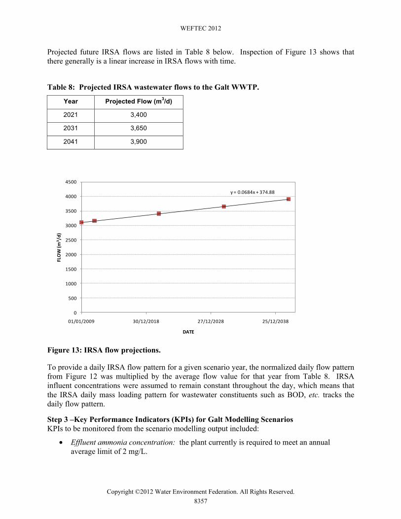
Once the data have been grouped into week and weekend days, they can be further simplified by averaging all of the week days and weekend days to result in typical average week and weekend day flow patterns, as shown in Figure 11 below.

To be conservative, the average weekday flow pattern was selected for use in the model-based scenario analysis. The normalized pattern is shown in detail in Figure 12 below.

0

500

1000

1500

2000

2500

3000

3500

4000

4500

0:00 4:00 8:00 12:00 16:00 20:00 0:00

Flow

(m3 /d)

Time (hours)

Individual Diurnal Patterns

Monday

Tuesday

Wednesday

Thursday

Friday

Saturday

Sunday

8355

WEFTEC 2012


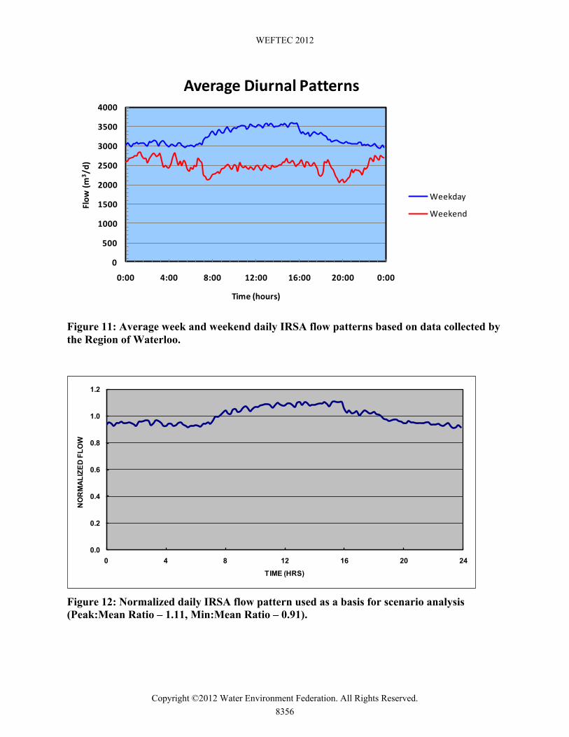
Figure 11: Average week and weekend daily IRSA flow patterns based on data collected by the Region of Waterloo.

Figure 12: Normalized daily IRSA flow pattern used as a basis for scenario analysis (Peak:Mean Ratio – 1.11, Min:Mean Ratio – 0.91).

0

500

1000

1500

2000

2500

3000

3500

4000

0:00 4:00 8:00 12:00 16:00 20:00 0:00

Flow

(m3 /d)

Time (hours)

Average Diurnal Patterns

Weekday

Weekend

0.0

0.2

0.4

0.6

0.8

1.0

1.2

0 4 8 12 16 20 24

NO

RM

ALIZ

ED F

LOW

...

TIME (HRS)

8356

WEFTEC 2012


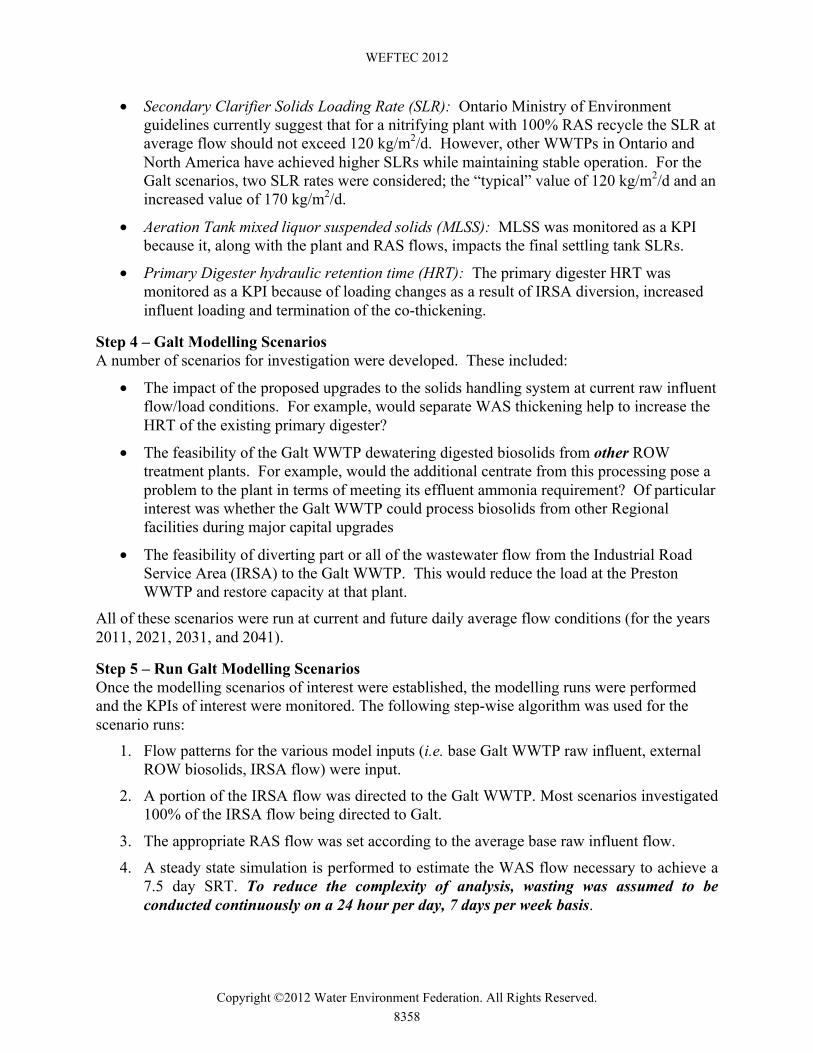
Projected future IRSA flows are listed in Table 8 below. Inspection of Figure 13 shows that there generally is a linear increase in IRSA flows with time.

Table 8: Projected IRSA wastewater flows to the Galt WWTP.

Year Projected Flow (m3/d)

2021 3,400

2031 3,650

2041 3,900

Figure 13: IRSA flow projections.

To provide a daily IRSA flow pattern for a given scenario year, the normalized daily flow pattern from Figure 12 was multiplied by the average flow value for that year from Table 8. IRSA influent concentrations were assumed to remain constant throughout the day, which means that the IRSA daily mass loading pattern for wastewater constituents such as BOD, etc. tracks the daily flow pattern.

Step 3 –Key Performance Indicators (KPIs) for Galt Modelling Scenarios KPIs to be monitored from the scenario modelling output included:

• Effluent ammonia concentration: the plant currently is required to meet an annual average limit of 2 mg/L.

y = 0.0684x + 374.88

0

500

1000

1500

2000

2500

3000

3500

4000

4500

01/01/2009 30/12/2018 27/12/2028 25/12/2038

FLOW (m

3 /d)

DATE

8357

WEFTEC 2012


• Secondary Clarifier Solids Loading Rate (SLR): Ontario Ministry of Environment guidelines currently suggest that for a nitrifying plant with 100% RAS recycle the SLR at average flow should not exceed 120 kg/m2/d. However, other WWTPs in Ontario and North America have achieved higher SLRs while maintaining stable operation. For the Galt scenarios, two SLR rates were considered; the “typical” value of 120 kg/m2/d and an increased value of 170 kg/m2/d.

• Aeration Tank mixed liquor suspended solids (MLSS): MLSS was monitored as a KPI because it, along with the plant and RAS flows, impacts the final settling tank SLRs.

• Primary Digester hydraulic retention time (HRT): The primary digester HRT was monitored as a KPI because of loading changes as a result of IRSA diversion, increased influent loading and termination of the co-thickening.

Step 4 – Galt Modelling Scenarios A number of scenarios for investigation were developed. These included:

• The impact of the proposed upgrades to the solids handling system at current raw influent flow/load conditions. For example, would separate WAS thickening help to increase the HRT of the existing primary digester?

• The feasibility of the Galt WWTP dewatering digested biosolids from other ROW treatment plants. For example, would the additional centrate from this processing pose a problem to the plant in terms of meeting its effluent ammonia requirement? Of particular interest was whether the Galt WWTP could process biosolids from other Regional facilities during major capital upgrades

• The feasibility of diverting part or all of the wastewater flow from the Industrial Road Service Area (IRSA) to the Galt WWTP. This would reduce the load at the Preston WWTP and restore capacity at that plant.

All of these scenarios were run at current and future daily average flow conditions (for the years 2011, 2021, 2031, and 2041).

Step 5 – Run Galt Modelling Scenarios Once the modelling scenarios of interest were established, the modelling runs were performed and the KPIs of interest were monitored. The following step-wise algorithm was used for the scenario runs:

1. Flow patterns for the various model inputs (i.e. base Galt WWTP raw influent, external ROW biosolids, IRSA flow) were input.

2. A portion of the IRSA flow was directed to the Galt WWTP. Most scenarios investigated 100% of the IRSA flow being directed to Galt.

3. The appropriate RAS flow was set according to the average base raw influent flow.

4. A steady state simulation is performed to estimate the WAS flow necessary to achieve a 7.5 day SRT. To reduce the complexity of analysis, wasting was assumed to be conducted continuously on a 24 hour per day, 7 days per week basis.

8358

WEFTEC 2012


5. The primary sludge flow and thickened WAS flows were adjusted to give concentrations in the region of 3.3 and 7%, respectively. Another steady state simulation was performed to establish the total Galt-WWTP internally-generated digested biosolids requiring dewatering.

6. The appropriate outflow pattern of the digested solids holding tank was determined, according to the biosolids inputs (i.e. Galt WWTP internally generated and external plant biosolids), number of centrifuges in operation and the operation shift length. In all cases examined, a single centrifuge operating at its maximum hydraulic capacity for a 14-hour shift was assumed. It is recognized that in some cases this can result in unnecessarily high peak centrate flows (which are equalized in the centrate holding tank) and non-optimal use of available digested solids holding tank volume; however, the goal of suggesting an optimized daily operation schedule was reserved for the future.

7. An appropriate outflow pattern was determined for the centrate holding tank, in order to achieve a degree of equalization of centrate return flows to the Galt WWTP main liquid treatment train.

8. A dynamic simulation was run for 4 days, to investigate the plant’s dynamic response under the given scenario.

Examples of output generated by the model are shown below.

Figure 14: Predicted dynamic effluent ammonia response for upgraded plant (dashed line of shows 2 mgN/L effluent permit limit) at 2021 raw influent and IRSA flows.

Figure 15: Predicted dynamic final settling tank solids loading rate response for upgraded plant (dashed lines shows 120 kg/m2/d design guideline limit and 170 kg/m2/d suggested upper limit) at 2021 raw influent and IRSA flows.

NH3-NFW Comp

Galt WWTP Effluent Ammonia

Jan-05-09Jan-04-09Jan-03-09Jan-02-09Jan-01-09

CO

NC

(mg/

L)

8

6

4

2

0

InstDaily Avg

Final Settling Tank #2 Solids Loading Rate

Jan-05-09Jan-04-09Jan-03-09Jan-02-09Jan-01-09

SLR

(kg/

m2/

d)

180

160

140

120

100

80

60

40

20

0

8359

WEFTEC 2012


Figure 16: Biosolids facility centrate holding tank daily volume fluctuation (dashed line shows tank maximum capacity) at 2021 raw influent and IRSA flows.

Some important findings from the scenario runs included:

• Upgrading the Galt WWTP to include WAS thickening (rather than co-thickening) results in less flow to the primary anaerobic digester. The lower flow in turn results in a longer digester hydraulic residence time (HRT) in comparison to current conditions; this should, along with other digester infrastructure upgrades, provide improved performance.

• Until 2011, the Galt WWTP appears to have the capacity to treat the base raw influent flow, as well as all of the IRSA flow, and process all biosolids volume from at least two other Region WWTPs (one medium-sized, one large).

• At 2021 conditions, the Galt WWTP liquid train appears to be capable of treating the base raw influent flow, all of the IRSA flow, but only process biosolids volume from one additional medium-sized Region WWTP.

• At 2031 conditions, the final clarifier SLR begins to become critical if all of the IRSA flow is diverted to the Galt WWTP. This conclusion highlights the importance of perhaps addressing this facet of plant operation via secondary clarifier stress testing, upgrades, or expansion.

• Under the future flow scenarios, the model-based analysis indicates that primary digester HRT may well become a limiting factor due to the generation of additional primary and secondary sludge from the increased plant loading. Based in part on this finding a decision was made to retrofit a secondary digester to a primary digester; this upgrade has recently been completed.

CONCLUSIONS

Linking several regional WWTPs in a model-based analysis allows for the examination of potential interactions and provides owners of these plants with information that (1) can be used to facilitate planning on a region-wide basis, (2) helps decision makers maximize the capacity of existing treatment plant infrastructure, (3) allows for sharing (where possible) of excess WWTP capacity, (4) achieves maximum benefit from new infrastructure, (4) provides a basis for more detailed work related to individual unit process optimization (e.g. collection of additional data around individual unit processes, stress testing, etc.), and (5) aids in the development of rational

Centrate Equalization Tank

Jan-05-09 00Jan-04-09 12Jan-04-09 00Jan-03-09 12Jan-03-09 00Jan-02-09 12Jan-02-09 00Jan-01-09 12Jan-01-09 00

VOLU

ME

(m3)

500

400

300

200

100

0

8360

WEFTEC 2012


plant upgrade strategies to accommodate future growth. This paper showed the results of such an exercise with the Galt WWTP serving as an example as to how decisions made at one plant could potentially affect future plans for several other Region WWTPs.

REFERENCES

Metcalf & Eddy (2003) Wastewater Engineering – Treatment and Reuse (4th Edition). ISBN 0-07-112250-8, McGraw-Hill, New York, NY, USA.

WERF (Water Environment Research Foundation) (2003) Methods for wastewater characterization in activated sludge modeling. Project 99-WWF-3, ISBN 1- 893664-71-6. Alexandria, Virginia.

8361

WEFTEC 2012


region-wide wastewater treatment plant modeling enhances...

Documents