1

Regional income inequality and happiness: Evidence from Japan

Takashi Oshio

Institute of Economic Research, Hitotsubashi University, Japan

Miki Kobayashi

Graduate School of Economics, Kobe University, Japan

Abstract

We investigated how regional income inequality is associated with the individual assessment of

happiness based on micro data from nationwide surveys in Japan. Our multilevel analysis using logit and

ordered logit models confirmed that individuals who live in areas of high inequality tend to report

themselves as less happy, even after controlling for various individual and regional factors. Notably, the

fact that happiness depends on not only income but also income inequality indicates the importance of

income redistribution for individual well-being. We also find that the association between regional

inequality and happiness is not uniform across the different levels of perceived happiness. Moreover, the

sensitivities of happiness to regional inequality differ substantially by key individual attributes such as

gender, marital status, level of education, occupational status, and political views. Among others, an

important finding for social policy is that those of unstable occupational status and those with a lower

level of education are more sensitive to regional inequality. Given the fact that these people tend to be

less happy than the others, this result points to the risk that regional inequality additionally reduces the

well-being of those under unfavorable socioeconomic conditions.

Keywords: Happiness, income inequality, multilevel analysis, Japan

Corresponding Author: Tel/Fax: +81-42-580-8658. Email: oshio@ier.hit-u.ac.jp.

2

1. Introduction

In recent years, following an influential paper by Wilkinson (1992) who showed that a more uneven

society has shorter life expectancy, the association between income distribution in society and individual

health has been increasingly studied. It is now widely recognized that an analysis based solely on

area-level data likely fails to disentangle the effects of individual factors from the pure effects of

regional income inequality. To explicitly address this issue, many researchers have employed a

multilevel analysis using multilevel data in the form of individual-level health outcome, set of

individual-level socioeconomic predictors, and area-level income inequality measures.

In these analyses of social epidemiology, self-rated health—that is, the subjective assessment of

health by an individual—has been a central variable to be focused upon in terms of its association with

income inequality. This health measure, which is often reported on a 3- or 5-point scale by surveyed

individuals, is considered as a reliable and pragmatic proxy of more objective health measures

(Burström and Fredlund 2001; Lundberg and Manderbacka 1996).

In effect, many empirical studies have been examining whether self-rated health is negatively

associated with regional income inequality. The results have been mixed in general, however, and it is

difficult to identify which factors explain the differences. As comprehensively surveyed by Subramanian

and Kawachi (2004) and Wilkinson and Pickett (2006), a substantial portion of the studies conducted

within the United States point to an association between wide income inequality and poor health, while

studies conducted outside the United States tend to have results that do not support the income

inequality hypothesis.

The association with regional income inequality is potentially an important issue to be addressed for

not only health but also happiness, the subjective assessment of which is often asked in social surveys

and investigated by empirical analysis of happiness studies. As in the case of self-rated health, multilevel

analysis is desirable when investigating the association between regional inequality and happiness. Most

3

of all, it is of interest to examine whether and to what extent individuals who live in areas of high

inequality tend to assess themselves as less happy, even after controlling for various factors including

household income.

Note that as surveyed by Frey and Stutter (2002), economists have been contributing large-scale

empirical analyses of the determinants of happiness in different countries and periods since the late

1990s. For example, Blanchflower and Osward (2004) and Easterlin (2001) showed that income

increases the level of happiness. Further, many economic researches—including Clark and Oswald

(1994), Korpi (1997), Winkelmann and Winkelmann (1998), Di Tella, MacCulloch, and Oswald

(2001)—have observed that unemployment or an unstable occupational status reduce subjective

well-being even after controlling for income. Marital status and relations with family members, other

acquaintances, and communities are also likely to affect happiness.

However, much is to be explored with regard to the association between regional inequality and

happiness. To our knowledge, little research has followed a seminal paper by Alesina, Di Tell, and

MacCulloch (2004), who observed that higher inequality in a society tends to reduce individual

happiness using the micro data of the United States and European countries. Following Alesina et al.

(2004), we employed a multilevel analysis based on micro data observed from large-scale nationwide

surveys in Japan, a non-Western advanced country. In this study, we controlled for a richer set of

individual and regional variables than Alesina et al. (2004), and examined how the results differ across

the different levels of perceived happiness. In addition, we investigated how the sensitivities to regional

inequality are modified by key individual attributes such as gender, age, level of education, income,

occupational status, and political views, expanding Alesina et al. (2004)’s analysis, which focused only

on income and political views.

An empirical analysis of the relationship between income inequality and happiness will potentially

have important implications for income redistribution in Japan as well as other advanced countries.

Japan is considered to be a relatively homogeneous society, with small levels of inequality. In reality,

4

however, its Gini coefficient is now higher than the OECD average, and the ratio of people with income

below the poverty line, which is half of the mean income, ranks as among the highest in the OECD

member countries (Förster and Mira d’Ecorle 2005). Indeed, many researchers raise concerns about

Japan’s trend of widening income inequality (Fukawa and Oshio 2007; Tachibanaki 2005). More

recently, Oshio and Kobayashi (2009) and Ichida et al. (2009) found that self-rated health is negatively

correlated with regional inequality or poverty in Japan. However, much is to be explored with regard to

the association between regional inequality and happiness, an issue which this study explicitly

addresses.

2. Data

Our analysis is based on micro data obtained from two nationwide surveys in Japan following Oshio

and Kobayashi (2009): (i) the Comprehensive Survey of Living Conditions of People on Health and

Welfare (CSLCPHW), which was compiled by the Ministry of Health, Labour, and Welfare, and (ii) the

Japanese General Social Survey (JGSS), which was compiled and conducted by the Institute of Regional

Studies at the Osaka University of Commerce in collaboration with the Institute of Social Science at the

University of Tokyo.

We used the CSLCPHW to construct prefecture-level variables and the JGSS to construct

individual-level variables. Japan has 47 prefectures, which are the basic units of local government and

administration in the country. The CSLCPHW had sufficiently large samples to obtain reliable estimates

of the Gini coefficient and the mean household income in each prefecture, but it had limited information

about demographic and socioeconomic factors at the individual level. In contrast, the JGSS had rich

individual-level information, but its sample size was not large enough to calculate prefecture-level

variables. By matching these data from the two datasets depending on where each respondent resided,

we conducted a multilevel analysis.

5

We collected micro data from the 2001, 2004, and 2007 CSLCPHWs, which include household

income data of 2000, 2003, and 2006, respectively. The CSLCPHW randomly selected 2,000 districts

from the Population Census divisions, which were stratified in each of the 47 prefectures according to

the population size. Next, all the households in each district were interviewed. The original sample size

was 30,386, 25,091, and 24,578 households (with a response rate of 79.5, 70.1, and 67.7 percent) in

2000, 2003, and 2006, respectively.

On the other hand, we collected data from 2000, 2003, and 2006 JGSSs to obtain detailed

information about the socioeconomic background of each respondent. The JGSS divided Japan into six

blocks and subdivided them according to the population size into three (in 2000 and 2003) or four (in

2006) groups. Next, the JGSS selected 300 (in 2000) or 489 (in 2003 and 2006) locations from each

stratum and randomly selected 12 to 15 individuals aged between 20 and 89 from each survey location.

The number of respondents was 2,893, 1,957, and 2,124 (with a response rate of 63.9, 55.0, and 59.8

percent) in 2000, 2003, and 2006, respectively.

In this empirical analysis, we eliminated the respondents aged below 25 and above 80, whose sample

sizes were limited; students; and those respondents whose key variables were missing. As a result, in our

estimation, a total of 4,452 individuals (aged between 25 and 80) responded (1,865 in 2000; 1,236 in

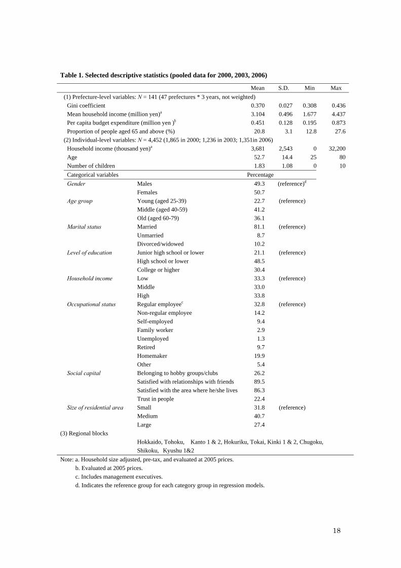
2003; and 1,351 in 2006). The summary statistics of all variables are presented in Table 1. In what

follows, we briefly explain the dependent and independent variables used in our empirical analysis.

The dependent variable is happiness. It is almost impossible to exactly define happiness, which is

multi-dimensional. Like many previous empirical studies of happiness, we focused on perceived

happiness that was expressed as a single item based on the survey results of the subjective assessment of

happiness. The JGSS asked the respondents to answer the question “How happy are you?” on a 5-point

scale with 1 being “happy” and 5 being “not happy.” The ratio of the responses in the three-year pooled

samples was 30.1, 33.2, 30.3, 5.1, and 1.3 percent, indicating that happiness is skewed towards the high

end in this survey. Happiness is often scored on a 3-point scale (for example, “very happy,” “fairly

6

happy,” and “not too happy”) in social surveys outside Japan, but we did not adjust the JGSS data into

three categories and used them as they were to avoid any bias due to arbitrary re-categorization. Instead,

in addition to estimating an ordered logit model with the original five categories, we tried to examine

how the different thresholds between “happy” and “not happy” affect the results of logit models.

Among all independent variables, the most important one is the Gini coefficient, which is one of the

most widely-used inequality measures. This coefficient ranges from zero to one, with zero indicating the

most equal distribution, and one indicating the most unequal distribution. We collected pre-tax

household income from the CSLCPHW and, like in most previous studies, equivalized it by dividing it

by the root of the number of household members. Then, we calculated the Gini coefficient for each

prefecture. Individuals who reside in the same prefecture in each survey year have a common Gini

coefficient.

To capture the association between happiness and regional inequality as precisely as possible, we

used various control variables at both the individual and prefecture levels, most of which we collected

from the JGSS. At the individual level, household income is one of the key variables. The JGSS asked

respondents to choose their household annual income for the previous year from among 19 categories.

We took the median value of each category, equivalized it, and evaluated it at the 2005 consumer prices.

Next, we divided income groups into three classes of almost the same size: “low” (with equivalized

household income below 2,449 thousand yen), “middle” (2,449 to 4,041 thousand yen), and “high”

(above 4,041 thousand yen).

At the individual level, we also considered gender: males and females; age: “young” (aged 25-39),

“middle” (40-59), and “old” (60-79); marital status: “married,” “unmarried,” and “divorced/widowed;”

and level of education: “junior high school or lower,” “high school,” and “college or higher.” In addition,

we considered occupational status, which was divided into eight categories: “regular employee”

(including management executives), “non-regular employee,” “self-employed,” “family worker,”

“unemployed,” “retired,” “homemaker,” and “other.” We also considered the number of children as an

7

explanatory variable, along with its squared value considering the possibility of its nonlinear

associations with happiness.

In addition to these widely-used control variables, we collected the following four aspects of an

individual’s relationship with or assessment of social capital from the JGSS, reflecting the previous

analysis of the association between social capital and happiness (Ram 2009 as a recent example): (i)

whether he/she is satisfied with his/her relationships with his/her friends (yes = 1); (ii) whether he/she is

satisfied with the place where he/she lives (yes = 1); (iii) whether he/she thinks that most people can be

trusted (yes = 1); and (iv) whether he/she belongs to any hobby group or club (yes = 1). For the first two

aspects, the JGSS asked respondents to choose from a 5-point scale with 1 denoting “satisfied” and 5

denoting “dissatisfied.” We categorized 1 and 2 as “yes.” Furthermore, we considered the size of the

area where a respondent lives. The JGSS asked each respondent to choose from a 3-point scale with 3

denoting the largest area. We used these answers as three categorized variables.

As for prefecture-level predictors, we controlled for (log-transformed) prefecture mean income, per

capita budget expenditure of the local government, and the proportion of people aged 65 and above.

Individuals who live in areas of higher average income and those who enjoy higher levels of government

spending are likely to feel happier than others; at the same time, however, the impact of the regional age

structure is unknown in general. Additionally, we included indicator variables for 12 regional blocks,

each of which comprised three to six prefectures (except Hokkaido) in order to control for the

unspecified characteristics of a region wider than a prefecture, and the unspecified characteristics for

three years to control for year-specific factors.

3. Methods

We employed five models to assess the association between regional inequality and happiness.

Model 1 was an ordered logit model that used five categories of reported happiness as an ordinal

8

variable. Model 2 was a logit model that allocated one to categories (5, 4, 3, 2) and zero to category (1).

In this model, the threshold between “happy” and “not happy” was placed at a very low level, as

category one (least happy) was only 1.3 percent of the entire sample. Model 3 was a logit model that

allocated one to categories (5, 4, 3) and zero to categories (2, 1). In the same way, Model 4 contrasted

categories (5, 4) and categories (3, 2, 1), and Model 5 contrasted category (5) and categories (4, 3, 2, 1).

The shares of the category “happy” in Models 3, 4, and 5 were 6.4, 36.7, and 69.9 percent, respectively.

Although a model of three categories is more widely used, an ordered logit model like Model 1 is

often employed by empirical studies. The appropriateness of this model depends on the parallel lines

(proportional odds) assumption—that is, the assumption that the coefficients are equal across categories.

It is possible, however, that the association with regional inequality differs between the lower and higher

levels of happiness. This is more likely to be the case especially when the observed distribution of

happiness is extremely skewed like the data from the JGSS. Hence, after estimating Model 1, we

conducted the approximate likelihood-ratio test of whether the coefficients are equal across categories,

and compared the estimated coefficients across four logit models—Models 2 to 5—with different

thresholds of happiness. In all estimations, we used JGSS-provided sampling weights and computed

robust standard errors to correct for potential heteroscedasticity.

In any case, however, the estimated associations between happiness and each explanatory variable

show only their averages across the different individual attributes. For certainty, we included key

individual attributes in the list of explanatory variables in logit model estimations, but the assumption

that the sensitivity of happiness to regional inequality is the same for all attributes may not hold. Hence,

we examined how it differs by key individual attributes such as gender, age, marital status, level of

education, household income, occupational status, and political views. For each attribute group, we

estimated the same logit model separately by each attribute and compared how the sensitivities to

regional inequality differed across the different attributes. For example, we estimated the coefficients on

the Gini coefficient separately for males and females to evaluate effect modification by gender. In

9

addition, we compared the statistical significance of the sensitivity to inequality within each attribute

group. There is no theory that tells which model we should choose from among Models 2 to 5 to

compare the results, but we used Model 4 because, as discussed below, it showed the most significant

association between regional inequality and health.

In this analysis, we condensed eight types of occupational status into three categories: regular

employees as “stable;” non-regular employees, self-employed persons, family workers, other types of

workers, and unemployed people as “unstable;” and retirees and homemakers as “out of labor force.” It

is questionable whether self-employment, which is 9.4 percent of the entire sample, should be

categorized as unstable. We considered self-employed persons as unstable, considering that their mean

income (3,869 thousand yen) was lower and its standard deviation (2,844 thousand yen) was higher than

those of regular employees (4,192 thousand and 2,066 thousand yen, respectively). Even if we

categorized self-employment as “stable,” the results were not substantially different.1

With respect to political views, the JGSS asked respondents to answer the question, “Where would

you place your political views on a 5-point scale?” with 1 being conservative and 5 being progressive.

We categorized the answers into “conservative” (1, 2), “neutral” (3), and “progressive” (4, 5). We did

not use political views as explanatory variables in the logit models, considering possible simultaneity

between them and happiness.

4. Findings

Before reporting the estimation results of logit models, Table 2 compares the means and standard

deviations of happiness by key individual attributes, when happiness is scored on a 5-point scale. We

notice the following findings with regard to the means of happiness: there is no substantial difference

between males and females; the young are happier than the middle-aged and old; married people are

1 The results are not reported but are available upon request.

10

more happier than the others; higher educational attainment makes people happier; higher income makes

people happier; people with unstable occupational status are less happy than the others; and the

politically conservative ones are happier than the others. These findings are reasonable in general but we

should be cautious in interpreting any causality from them especially for marital status, occupational

status, and political views. People may remain married because they are happy, may be unemployed

because they are not satisfied with their jobs, and may be politically conservative because they are

satisfied with their life.

Table 3 summarizes the estimation results from Model 1 (an ordered logit model with five categories

of happiness), Models 2 to 5 (logit models with different thresholds between “happy” and “not happy”).

We first notice that in Model 1, the coefficient on the Gini coefficient is negative and significant at the

10 percent significance level, confirming a negative, albeit modest, association between regional

inequality and happiness. This result is notable in that it is obtained even after controlling for household

income, which, as expected, is found to be positively associated with happiness. We also find that young

and married people are happier than the others, while the unemployed are less happy. At the prefecture

level, higher spending by the local government adds to happiness. Another notable finding from Model 1

is that all the four variables that indicate the individual relationship with social capital show positive and

strongly significant associations with happiness. This highlights the importance of social capital for

individual well-being.

It should be noticed, however, that ordered logit models generally assume that the coefficients are

equal across categories. This assumption may not hold in this case, especially given an extremely

skewed distribution of perceived happiness. In fact, the approximate likelihood-ratio test of whether the

coefficients are equal across categories revealed that the assumption can be rejected at the one percent

significance level. 2 Hence, we estimated four logit models—Models 2 to 5—with different

categorizations of “happy” and “unhappy.” We also estimated a generalized ordered logit model by 2 In fact, χ2 (41) was 143.96, well above 74.75, the critical value at the one percent significance level, where 41 was

the number of independent variables.

11

relaxing the parallel lines assumption, and obtained results that were not much different from those in

Models 2 to 5.3

Three findings are noteworthy from these logit models. First, the coefficient of the Gini coefficient is

negative and significant (at the five percent significance level) only for Model 4. In this model,

categories (5, 4), which are 63.3 percent of the entire sample, were defined as “happy.” The coefficients

on the Gini coefficient are positive in Models 2 and 3 and negative in Model 5, but in all of these, the

coefficients are insignificant and the absolute values are smaller than that in Model 4.

Second, the statistical significance and sizes of the estimated coefficients have almost the same

patterns in Models 1 and 4, while the coefficient of the Gini coefficient is more significant and larger in

Model 4. Combined with the first finding, this suggests that the assessment of happiness between

categories (5, 4) and (3, 2, 1) largely determines its overall assessment across the five ordered

categories.

Third, some predictors are significantly associated with happiness across all models, while others are

not. For example, all four variables related to social capital are positively and significantly associated

with happiness in most cases, confirming its positive and stable associations with individual well-being

across the various levels of happiness. Marital status also shows stable associations with happiness;

married people are happier than the others in all models. In line with expectations, household income

also matters in most cases. However, age and level of education matter only in Models 3 and 4, while

occupational status matters only in Models 1 and 2 and that too substantially. These findings underscore

that the association between individual attributes and happiness differ substantially at the different levels

of perceived happiness. In addition, the fact that occupational status is a crucial determinant of

individual well-being at a lower level of perceived happiness indicates the need for enhancing job

opportunities and job security.

An important problem in the estimations based on these models is that the estimated sensitivity of

3 The result of the generalized ordered logit model is available upon request.

12

happiness to regional inequality, which is based on the entire sample, only shows its average across

different attributes. We cannot rule out the case that only a certain portion of the respondents with

certain attributes are sensitive to regional inequality. Table 4 compares the coefficients on the Gini

coefficient, along with their robust standard errors and p-values, obtained from the separately estimated

Model 4 by each category of individual attributes. The table also reports the odds ratios for reporting

categories 4 and 5 in response to a one-standard deviation increase in the Gini coefficient, along with its

95 percent significance intervals.

By comparing the coefficients and odds ratios, we obtain the following findings with regard to the

sensitivity to regional inequality when assessing happiness: females are more sensitive than males; there

is no substantial difference across age groups; married people are less sensitive than others; those who

finished education at junior high school or lower are more sensitive than others; those who belong to the

highest income class are modestly more sensitive than others; unstable occupational status makes people

most sensitive; and politically neutral individuals are more sensitive than others.4

We also find that unless there are no substantial differences across categories (that is, age and

household income), regional inequality tends to be significant only for the category that is most sensitive

to inequality within each category group. These results confirm that the sensitivity to regional inequality

is not uniform across the individuals of different attributes.5

5. Discussion and conclusion

We examined how regional inequality is associated with the individual assessment of happiness

4 Alesina et al. (2004) pointed out that the poor and left-wingers are sensitive to inequality in Europe, while in the

United States, the happiness of these groups is uncorrelated with inequality. 5 We should be cautious in interpreting these results, however, because comparisons of the estimated coefficients

on the Gini coefficient do not make sense if the Gini coefficient is distributed differently between categories. To check this, we applied the Kolmogorov-Smirnov tests between each category and the remaining one or two categories in each category group. We found that the null hypothesis that the Gini coefficient is distributed differently between categories cannot be rejected at the five percent significance level for two cases: between individuals who graduated from college or higher institutions and others, and between low income-individuals and others.

13

based on micro data from nationwide surveys in Japan. Our multilevel analysis using logit and ordered

logit models confirmed that individuals who live in areas of high inequality tend to report themselves as

less happy, even after controlling for various individual and regional factors. Notably, the fact that

happiness depends on not only income but also income inequality indicates the importance of income

redistribution for individual well-being.

This result is parallel to that from many empirical studies of social epidemiology that observed a

negative association between regional inequality and self-rated health, which is one of the key subjective

outcomes of individual well-being. The observed association between regional inequality and self-rated

health observed in this study is also reasonable, considering the close relationship with happiness and

health.6

However, there is no well-established theory that explains why regional inequality is associated

with individual well-being. One plausible explanation is that individuals may have a certain ideal picture

of income distribution and that a deviation from it—especially in the form of wider inequality or more

poverty—may reduce happiness. An ideal income distribution is, however, likely to differ among

individuals of different attributes; people under unfavorable socioeconomic conditions are probably

more inequality-averse. An alternative explanation is that individuals may regard observed income

inequality as a proxy for the uncertainty about future income. The more they are risk-averse, the more

they are sensitive to income inequality. These two views are closely related and not exclusive with each

other because inequality aversion and risk aversion are identical at least to some extent. Our estimation

results look modestly more consistent with the former view, but they do not reject the latter.

It should be noted, however, that any association between regional inequality and happiness is not

uniform across the different levels of happiness. Our empirical analysis based on ordered logit and

ordered logit models highlighted this. On the one hand, we observed a negative, albeit modest,

6 For example, Perneger, Hudelson, and Bovier (2004) reported that healthier individuals tend to feel happier, while

Pettit and Kline (2001) showed that a better assessment of happiness can lead to a higher level of self-rated health.

14

association between the two variables, when we estimated an ordered logit model that used five ordered

categories of happiness. On the other hand, we did not find a significant association between them, when

we estimated logit models that placed the threshold of happiness at relatively lower or higher levels of

happiness.

The association between individual attributes and happiness also differs across the different levels of

happiness. Occupational status matters at a lower level of happiness, while age and level of education

matter at a higher level. In contrast, social capital shows a positive and significant association for all

models, suggesting that it is potentially a powerful and reliable buffer against any negative pressure of

regional inequality and other socioeconomic factors on individual well-being.

Finally, we found that the sensitivities of happiness to regional inequality differ substantially by key

individual attributes such as gender, marital status, level of educational attainment, occupational status,

and political views. An important finding for social policy is that those of unstable occupational status

and with lower level of education are more sensitive to regional inequality. Given the fact that they tend

to be less happy than others, this result points to the risk that regional inequality further reduces the

well-being of those under unfavorable socioeconomic conditions.

We recognize that this analysis has various limitations. Most of all, it deals with happiness only as a

single item based on the survey results of its subjective assessment. Given the multi-dimensional feature

of happiness, the validity of perceived happiness observed from surveys should be addressed further.

Second, as is often the case with a multilevel analysis of this type, pathways or a mediation process from

regional inequality with respect to happiness at an individual level should be investigated further. Third,

we disregarded the possibility that perceived happiness changes individual characteristics, which we

assumed to be exogenous. These issues should be researched in the future.

15

Acknowledgements

The data from Comprehensive Survey of Living Conditions of People on Health and Welfare were

made available by the Ministry of Health, Labor and Welfare of Japan under the Kosei Rodo Kagaku

Kenkyuhi Joseikin Project entitled “Research on Social Security Benefit and Contributions with

reference to Income, Asset and Consumption” in 2008 (No. 1211006). The micro data from this survey

were accessed and analyzed exclusively by Takashi Oshio.

The data for the secondary analysis, the Japanese General Social Survey (JGSS), were provided by

the Social Science Japan Data Archive, Information Center for Social Science Research on Japan,

Institute of Social Science, University of Tokyo. The JGSSs are designed and carried out by the JGSS

Research Center at the Osaka University of Commerce (Joint Usage/Research Center for Japanese

General Social Surveys accredited by the Minister of Education, Culture, Sports, Science and

Technology) in collaboration with the Institute of Social Science at the University of Tokyo.

We appreciate the financial support provided by the Grant-in-Aid for Scientific Research on Priority

Areas (21119004) and the Grant-in-Aid for Scientific Research (B) (21330057).

16

References

Alesina A., Di Tell, R., MacCulloch, R. (2004). Inequality and happiness: Are Europeans and

Americans different? Journal of Public Economics, 88(9–10), 2009–2042.

Blanchflower, D.G., Oswald, A.J. (2004). Well-being over time in Britain and the USA. Journal of

Public Economics, 88(7–8), 1359–1386.

Burström, B., Fredlund P. (2001). Self-rated health: is it a good predictor of subsequent mortality among

adults in lower as in higher social classes? Journal of Epidemiology and Community Health,

55(11), 836–840.

Clark, A.E., Oswald, A.J. (1994). Unhappiness and unemployment. Economic Journal, 104(424),

648–659.

Di Tella, R., MacCulloch, R.J., Oswald A.J. (2001). Preferences over inflation and unemployment:

Evidence from surveys of happiness. American Economic Review, 91(1), 335–341.

Easterlin, R.A. (2001). Income and happiness: Towards a unified theory. Economic Journal, 111(473),

465–484.

Förster, M., Mira d’Ecorle, M. (2005). Income distribution and poverty in OECD countries in the second

half of the 1990s. OECD Social, Employment and Migration Working Paper, 22.

Frey, B.S., Stutter, A. (2002). What can economists learn from happiness research? Journal of Economic

Literature, 40(2), 402–435.

Fukawa, T., Oshio, T. (2007). Income inequality trends and their challenges to redistribution policies in

Japan. Journal of Income Distribution, 16(3–4), 9–30.

Ichida, Y., Kondo K., Hirai, H., Hanibuchi, T., Yoshikawa, G., Murata, C. (2009). Social capital, income

inequality and self-rated health in Chita peninsula, Japan: A multilevel analysis of older people in

25 communities. Social Science & Medicine, 69(4), 489–499.

Korpi, T. (1997). Is well-being related to employment status? Unemployment, labor market policies and

subjective well-being among Swedish youth. Labour Economics, 4(2), 125–147.

17

Lundberg, O., Manderbacka, K. (1996). Assessing reliability of a measure of self-rated health.

Scandinavian Journal of Social Medicine, 24(3), 218–224.

Oshio, T., Kobayashi, M. (2009). Income inequality, area-level poverty, perceived aversion to inequality

and self-rated health in Japan. Social Science & Medicine, 69(3), 317–326.

Perneger, T.V., Hudelson, P.M., Bovier, P.A. (2004). Health and happiness in young Swiss adults,

Quality of Life Research, 13(1), 171–178.

Pettit, J.W., Kline, J.P. (2001). Are happy people healthier? The specific role of positive affect in

predicting self-reported health symptoms. Journal of Research in Personality, 35(4), 521–536.

Ram, R. (2009). Social capital and happiness: Additional cross-country evidence, Journal of Happiness

Studies, doi: 10.1007/s10902-009-9148-3.

Subramanian, S.V., Kawachi, I. (2004). Income inequality and health: What have we learned so far?

Epidemiologic Reviews, 26(1), 78–91.

Tachibanaki, T. (2005). Confronting income inequality in Japan. Cambridge: MIT Press.

Wilkinson, R.G. (1992). Income distribution and life expectancy. British Medical Journal, 304(6820),

165–168.

Wilkinson, R.G., Pickett, E.K. (2006). Income inequality and health: A review and explanation of the

evidence. Social Science & Medicine, 62(7), 1768–1784.

Winkelmann, L., Winkelmann, R. (1998). Why are the unemployed so unhappy? Evidence from panel

data. Economica, 65(257), 1–15.

18

Table 1. Selected descriptive statistics (pooled data for 2000, 2003, 2006)

Mean S.D. Min Max

(1) Prefecture-level variables: N = 141 (47 prefectures * 3 years, not weighted)

Gini coefficient 0.370 0.027 0.308 0.436

Mean household income (million yen)a 3.104 0.496 1.677 4.437

Per capita budget expenditure (million yen )b 0.451 0.128 0.195 0.873

Proportion of people aged 65 and above (%) 20.8 3.1 12.8 27.6

(2) Individual-level variables: N = 4,452 (1,865 in 2000; 1,236 in 2003; 1,351in 2006)

Household income (thousand yen)a 3,681 2,543 0 32,200

Age 52.7 14.4 25 80

Number of children 1.83 1.08 0 10

Categorical variables Percentage

Gender Males 49.3 (reference)d

Females 50.7

Age group Young (aged 25-39) 22.7 (reference)

Middle (aged 40-59) 41.2

Old (aged 60-79) 36.1

Marital status Married 81.1 (reference)

Unmarried 8.7

Divorced/widowed 10.2

Level of education Junior high school or lower 21.1 (reference)

High school or lower 48.5

College or higher 30.4

Household income Low 33.3 (reference)

Middle 33.0

High 33.8

Occupational status Regular employeec 32.8 (reference)

Non-regular employee 14.2

Self-employed 9.4

Family worker 2.9

Unemployed 1.3

Retired 9.7

Homemaker 19.9

Other 5.4

Social capital Belonging to hobby groups/clubs 26.2

Satisfied with relationships with friends 89.5

Satisfied with the area where he/she lives 86.3

Trust in people 22.4

Size of residential area Small 31.8 (reference)

Medium 40.7

Large 27.4

(3) Regional blocks

Hokkaido, Tohoku, Kanto 1 & 2, Hokuriku, Tokai, Kinki 1 & 2, Chugoku,

Shikoku, Kyushu 1&2

Note: a. Household size adjusted, pre-tax, and evaluated at 2005 prices.

b. Evaluated at 2005 prices.

c. Includes management executives.

d. Indicates the reference group for each category group in regression models.

19

Table 2 Means and standard deviations of happiness (5-point scale)

Happiness Mean S. D. Number of obs.

(happy = 5, 4, 3, 2, 1 = unhappy)

Total 3.86 (0.95) 4,452

Gender Male 3.83 (0.94) 2,197 Female 3.88 (0.96) 2,255

Age

Young 3.94 (0.94) 1,012 Middle 3.82 (0.94) 1,834 Old 3.85 (0.96) 1,606

Marital status

Married 3.94 (0.90) 3,609 Unmarried 3.40 (1.02) 386 Divorced/widowed 3.56 (1.10) 456

Level of education

Junior high school or lower 3.76 (1.02) 940 High school 3.84 (0.96) 2,158 College or higher 3.95 (0.87) 1,354

Household income

Low 3.72 (1.03) 1,482 Middle 3.83 (0.91) 1,468 High 4.03 (0.88) 1,503

Occupational status

Stablea 3.87 (0.90) 1,658

Unstableb 3.78 (1.01) 1,476

Out of labor forcec 3.93 (0.94) 1,318

Political view

Progressive 3.83 (0.93) 991 Neutral 3.81 (0.95) 2,168

Conservative 3.97 (0.94) 1,227 Note: a = regular employee; b = self-employed + family worker + unemployed + other;

c = retired + homemaker.

20

Table 3. Estimated associations of independent variables with happiness

Ordered logit model Logit models

Dependent variable: happiness (happy = 5, 4, 3, 2, 1 = unhappy) Model 1 Model 2 Model 3 Model 4 Model 5

5, 4, 3, 2, 1 (5, 4, 3, 2) vs. (1) (5, 4, 3) vs. (2, 1) (5, 4) vs. (3, 2, 1) (5) vs. (4, 3, 2, 1)

Coef. Robust

S.E. Coef.

Robust S.E.

Coef. Robust

S.E. Coef.

Robust S.E.

Coef. Robust

S.E.

Gini coefficient -2.89 (1.65) * 1.15 (5.99) 0.49 (3.60) -3.88 (1.92) ** -2.31 (2.02)

Gender: Female 0.14 (0.08) * 0.72 (0.43) * 0.16 (0.18) 0.10 (0.09) 0.15 (0.10)

Age group: Middle -0.55 (0.08) *** -0.34 (0.45) -0.30 (0.19) -0.61 (0.10) *** -0.56 (0.10) ***

Old -0.35 (0.10) *** 0.64 (0.60) 0.19 (0.24) -0.48 (0.12) *** -0.40 (0.12) ***

Marital status: Unmarried -1.11 (0.14) *** -2.15 (0.65) *** -1.35 (0.27) *** -1.18 (0.16) *** -0.93 (0.19) ***

Divorced/widowed -0.62 (0.11) *** -2.39 (0.42) *** -1.19 (0.20) *** -0.54 (0.12) *** -0.45 (0.13) ***

Level of education: High school -0.01 (0.09) -0.29 (0.44) -0.18 (0.20) 0.02 (0.10) -0.08 (0.10)

College or higher 0.08 (0.10) 0.30 (0.56) 0.06 (0.24) 0.33 (0.12) *** -0.20 (0.12) *

Household income: Middle -0.01 (0.08) 0.79 (0.46) * 0.39 (0.17) ** 0.01 (0.09) -0.19 (0.10) *

High 0.44 (0.09) *** 0.56 (0.45) 0.69 (0.20) *** 0.52 (0.10) *** 0.30 (0.10) ***

Occupational status: Non-regular employee -0.13 (0.11) -1.17 (0.64) * -0.13 (0.25) -0.21 (0.12) * 0.00 (0.13)

Self-employed 0.07 (0.11) -1.25 (0.66) * -0.20 (0.27) 0.01 (0.13) 0.16 (0.13)

Family worker -0.16 (0.18) -2.30 (0.71) *** 0.04 (0.44) -0.21 (0.22) -0.12 (0.23)

Unemployed -1.08 (0.39) *** -3.16 (0.70) *** -1.90 (0.35) *** -0.37 (0.29) -0.27 (0.36)

Retired 0.08 (0.13) -1.49 (0.72) ** -0.02 (0.31) 0.02 (0.15) 0.23 (0.15)

Homemaker 0.12 (0.11) -0.82 (0.71) -0.03 (0.25) 0.13 (0.13) 0.19 (0.13)

Other 0.05 (0.17) -1.94 (0.58) *** -0.38 (0.29) 0.03 (0.19) 0.24 (0.19)

Social capital: Belonging to hobby groups/clubs 0.21 (0.07) *** -0.40 (0.38) 0.15 (0.17) 0.20 (0.08) ** 0.22 (0.08) ***

Satisfied with relationships with friends 0.91 (0.11) *** 1.34 (0.34) *** 1.15 (0.18) *** 0.79 (0.11) *** 0.81 (0.14) ***

Satisfied with the area where he/she lives 0.49 (0.10) *** 0.63 (0.36) * 0.89 (0.17) *** 0.56 (0.10) *** 0.18 (0.11)

Trust in people 0.52 (0.07) *** 1.48 (0.67) ** 0.60 (0.21) *** 0.55 (0.09) *** 0.53 (0.08) ***

Size of residential area: Medium 0.10 (0.09) 0.09 (0.41) 0.19 (0.19) 0.19 (0.09) ** 0.11 (0.10)

Large -0.02 (0.02) 0.66 (0.46) -0.05 (0.20) 0.18 (0.10) * -0.03 (0.10)

Number of children 0.16 (0.08) * -0.31 (0.44) 0.31 (0.15) ** 0.06 (0.10) 0.10 (0.09)

Number of children squared 0.06 (0.08) 0.02 (0.09) -0.09 (0.03) *** 0.00 (0.02) -0.01 (0.02)

21

Log of mean household income 0.06 (0.51) -1.69 (2.74) -0.67 (1.11) 0.39 (0.57) -0.26 (0.61)

Per capita budget expenditure 1.04 (0.45) ** -1.39 (2.75) -1.20 (1.01) 1.35 (0.53) ** 1.05 (0.55) *

Proportion of people aged 65 and above -0.02 (0.02) 0.19 (0.14) 0.10 (0.05) * -0.04 (0.03) -0.02 (0.03)

Number of observations 4,442 4,442 4,442 4,442 4,442

Pseudo R2 0.0518 0.2920 0.1708 0.0878 0.0510

Log likelihood -5447.01 -2040.58 -8630.98 -2648.77 -2579.21

Note. 1. Italics denote the category. See Table 1 for the reference group for each category (except for social capital).

2. All models include indicator variables for regional blocks and survey years.

3. For the ordered logit model, the parallel line assumption was rejected at the one percent significance level: χ2 (41) = 143.96, where 41 is the number of independent variables.

4. *** p < 0.01, ** p < 0.05, * p < 0.1.

22

Table 4. Comparing estimated sensitivities of happiness to regional inequality by key individual attributes Coef. Robust S.E. p-value OR 95% CI

Total -3.88 (0.94) 0.044 0.90 [0.85 - 0.95]

Gender

Male -0.82 (2.80) 0.770 0.98 [0.84 - 1.14] Female -7.56 (2.67) 0.005 0.81 [0.70 - 0.94]

Age

Young -5.11 (4.40) 0.246 0.87 [0.69 - 1.10]

Middle -3.39 (2.99) 0.258 0.91 [0.78 - 1.07]

Old -4.71 (2.98) 0.113 0.88 [0.75 - 1.03]

Marital status

Married -2.63 (2.15) 0.222 0.93 [0.83 - 1.04]

Unmarried -10.95 (7.62) 0.150 0.74 [0.49 - 1.12]

Divorced/widowed -15.75 (6.84) 0.021 0.65 [0.45 - 0.94]

Level of education

Junior high school or lower -10.49 (4.07) 0.010 0.75 [0.60 - 0.93]

High school -2.30 (2.69) 0.393 0.94 [0.81 - 1.08]

College or higher* -3.44 (3.75) 0.359 0.91 [0.74 - 1.11]

Household income

Low* -3.25 (2.98) 0.277 0.91 [0.78 - 1.07]

Middle -3.40 (3.41) 0.319 0.91 [0.76 - 1.09]

High -4.87 (3.66) 0.183 0.88 [0.72 - 1.07]

Occupational status

Stablea 2.74 (3.33) 0.411 1.08 [0.90 - 1.29]

Unstableb -15.13 (3.38) 0.000 0.66 [0.55 - 0.79]

Out of labor forcec -3.29 (3.38) 0.331 0.91 [0.76 - 1.10]

Political view

Progressive 1.33 (4.44) 0.765 1.04 [0.83 - 1.32]

Neutral -5.95 (2.79) 0.033 0.85 [0.73 - 0.99]

Conservative -4.79 (3.71) 0.197 0.88 [0.72 - 1.07]

Note. 1. This table compares the estimated coefficients on the Gini coefficient in Model 4 for each category.

2. OR indicates the odds ratios for reporting 3 (against 1 and 2) in response to a one-standard -deviation increase in the Gini coefficient (0.027). 95% CI indicates its 95% confidence interval.

3. a = regular employee; b = self-employed + family worker + unemployed + other; c = retired + homemaker. 4. The null hypothesis that the distribution of the Gini coefficient differs between the category with * and

the other two categories in the same category group cannot be rejected at the 5% significance level.