Regional Integration: An Empirical Assessment of Russia

Daniel Berkowitz* and David N. DeJong**

Department of Economics University of Pittsburgh

Pittsburgh, PA 15260 (Berkowitz: Davidson Institute; University of Michigan)

This revision: February 2003

Suggested Running Head: “Regional Integration” JEL Classifications: P22, R1

* (412) 648-7072; dmberk@pitt.edu **(412) 648-2242; dejong@pitt.edu For their many valuable comments, we are grateful to an anonymous referee, Alberto Alesina, Jan Brueckner, Alessandra Casella, Konstantin Glushchenko, Torsten Persson, Daniel Treisman, and seminar participants at the CEPR/WDI Conference on Transition Economics; Columbia University; the Nuffield College, University of Oxford; the Pittsburgh-Carnegie Mellon applied microeconomics workshop; the Stockholm School of Economics; the University College of London; the University of Illinois; the University of Virginia; WIDER (Helsinki); and the National Academy of Sciences symposium on Conflict in Multiethnic Societies held in Moscow. We are also grateful to Yadviga Semikolenova for providing research assistance, and to the National Council for Eurasian and East European Research for financial support under Contract No.816-2g. The usual disclaimer applies.

1

Regional Integration: An Empirical Assessment of Russia

Abstract

Using a statistical model of commodity trade, we quantify the evolution of regional economic integration within Russia during 1995-1999, and explore potential determinants of this evolution. Our integration measure exhibits rich regional variation that, when aggregated to the national level, fluctuates substantially over time. In accounting for this behavior, we draw in part on theoretical models that emphasize the potential role of openness to international trade and regional disparities in income in threatening economic integration. Controlling for a host of additional regional- and national-level variables, we find a strong negative correspondence between openness to international trade and internal economic integration.

Keywords: openness to international trade; regional income disparities; inflation

volatility; economic integration.

2

I. Introduction A striking feature of the economic transitions undertaken by many post-socialist countries is the

struggles they have encountered in preserving economic and political integration. Regarding economic

integration, for example, following the economic reforms established by China in 1978, many regions

within China erected inter-regional trade barriers and engaged in trade wars with each other (e.g., see

Young [37] and references therein). Also, following the federal imposition of economic reforms in the

early 1990s, many regional politicians within Russia violated federal laws mandating the free flow of

goods across regions by taking such actions as the erection of border controls, the physical limitation of

cross-border trade, and the issuance of local coupons designed to exclude non-residents from consuming

locally produced goods (e.g., see Freinkman et al. [11] and Mitchneck [22]). Regarding political

integration, economic transition has often coincided with political disintegration. For example, during the

1990s the former Czechoslovakia split into two independent countries, the former Yugoslavia split into

six countries, and the Former Soviet Union (FSU) split into fifteen independent countries. Furthermore,

regions in many of the newly independent countries within the FSU such as Azerbaizhan, Georgia,

Moldova, Russia and the Ukraine have subsequently taken measures that have undermined the political

integration of their countries. For example, starting in the early 1990s, many ethnic regions within Russia

engaged in separatist activities that included declarations of sovereignty, refusals to send conscripts to the

federal army, assertions of the right to print their own currencies, and assertions of control over natural

resources that had been under federal jurisdiction. This in turn has encouraged many non-ethnic regions

to engage in similar acts of separatism (Treisman [32,33]). Perhaps most notably, many Russian regions

have chosen to delay or even withhold mandatory tax payments owed to the federal government. In

particular, the massive decline in federal tax receipts between 1992 and 1998 resulted in large part from

the growth in late payments and non-payments from regional budgets (OECD [23, 24]; Treisman [34]).

In order to better understand forces that may be responsible for undermining economic

integration in post-socialist nations, we use a rich regional data that enables us to quantify and attempt to

account for patterns of regional economic integration observed within Russia. We quantify economic

integration between 1995-1999 using a statistical model of commodity trade developed by Engel and

Rogers [9] and Parsley and Wei [26]. The model is designed to evaluate whether the behavior of

commodity prices in a particular region vis-à-vis the region’s potential trading partners is consistent with

the behavior one would expect to observe if the region in question was actually open to regional trade.

We use the model to produce a yes/no signal regarding openness to domestic trade for 72 of Russia’s now

89 regions (complete data on the remaining regions are unavailable). We produce such a signal for each

region on a monthly basis. Summing signals over regions yields an aggregate measure of the proportion

3

of regions deemed to be integrated at a given point in time; the aggregate measure we obtained is

illustrated in Figure 1.

There is striking temporal variation in the aggregate characterization of integration provided in

Figure 1. Beginning in 1995, an initial period of widespread integration gradually gave way to a period of

disconnectedness in 1996 and 1997, which seems to have subsided by 1998. At the disaggregated level,

there is also striking variation in patterns of integration observed across regions. For example, the Sakha

Republic was isolated from its internal trading partners throughout the sample period; Krasnoyarsk and

Udmurtia maintained strong internal connections throughout the period; Ivanovo was integrated initially

but subsequently became isolated; and Arkhangelsk was isolated initially and then gradually became

integrated.

In seeking to account for these patterns of economic integration, we rely in part on guidance from

theoretical characterizations of economic and political integration. In particular, Alesina et al. [1] and

Casella [6] present models in which trade liberalization can pose a threat to political integration by

making regions within a political union less reliant on fellow members as trading partners, and also as

sources of financing for public goods and institutions. In the case of Russia, trade liberalization

potentially poses a particularly important threat because, as noted by Ericson [10], pitfalls associated with

inter-regional trading, such as late payments and high and arbitrary federal and regional taxes, are

particularly severe. In addition, Bolton and Roland [5] caution that disparities in regional incomes can

weaken internal political ties in regions that are sufficiently poor and sufficiently rich. If a region is

sufficiently rich, it has the fiscal capacity to finance its own public goods independently, and at some

point may lose its willingness to subsidize the provision of public goods in the rest of the country. In

contrast, if a region is sufficiently poor, it may break off from the federation if it becomes dissatisfied

with the extent of federal redistribution it receives.

In many respects, Russia offers a particularly useful laboratory for evaluating the influence of

these potential sources of disintegration. During its transition, it has made great strides in opening its

economy to world markets; and it has experienced dramatic and persistent disparities in standards of

living across regions. Our purpose is to investigate empirical links between these conditions and the

patterns of economic integration noted above.

We use a reduced-form statistical framework to characterize economic integration at the regional

level. This involves modeling regions as individual entities that base decisions regarding participation in

trade with domestic partners in a given time period on a collection of region-specific and national-level

variables (described in detail in Section III). National-level variables consist of annual measures of

openness to international trade and inflation volatility, as well as variables that quantify strike activity and

4

the pervasiveness of poverty at the aggregate level.1 Region-specific variables are of two types: time-

varying and fixed. The time-varying measures control for regional patterns of poverty and fluctuations in

transport costs (which are included to quantify a potential detriment to domestic trade). The fixed

variables include two measures of income disparities (one that measures the disparity between regional

and national median incomes for rich regions, and one for poor regions). They also include regional

measures of initial income, education levels, and language diversity.

Our analysis indicates the presence of a strong negative link between openness to international

trade and economic integration within Russia. Under our baseline estimates, a one-standard-deviation

increase in our aggregate measure of openness to trade is associated with a 6-7% decline in the

probability that a region will be linked with its internal trading partners in any given period. Results

regarding regional income disparities are mixed. The Bolton-Roland model suggests that a region will

tend to have a lower propensity towards integration as the absolute difference between its median income

and the national median income increases. We find that this pattern holds only for regions with relatively

low median incomes. However, we do find strong negative and significant links between integration and

initial income levels and initial educational levels; thus there is some evidence of the negative association

between regional prosperity and integration one would expect in light of the Bolton-Roland model.

Finally, we also find a negative link between inflation volatility and integration, but the link is of

marginal statistical significance.

A substantial literature has arisen out of attempts to measure and explain economic integration in

post-socialist economies. Gardner and Brooks [12] and De Masi and Koen [7] studied this problem for the

early phase of Russia’s reform and found that large differences in inter-regional prices could not be

explained by distance. Since arbitrage opportunities for tradable goods do not persist in inter-regional

markets within developed countries, both studies concluded that Russia’s market integration was limited.

In Berkowitz and DeJong [2] we found that a reason for this high inter-regional price dispersion was the

behavior of pro-Communist and anti-market regions. In Berkowitz and DeJong [3], we conducted an

aggregate-level study that sought to account for the dynamic behavior of economic integration in Russia;

we found that aggregate measures of economic integration exhibit a strong negative relationship with

openness to international trade, and have no significant correspondence with aggregate inflation volatility.

Young [37] documented and explained economic disintegration in China following its 1978 reforms, and

noted that it too coincided with an increased openness to world markets. Finally, in a detailed econometric

1 Regarding inflation and inflation volatility, e.g., Sheshinski and Weiss [28, 29] show theoretically that the presence of menu costs can cause inflation and inflation volatility to exacerbate gaps between regional differences in relative prices. Also, there is a large empirical literature that explores such effects (e.g., Lach and Tsiddon [21]).

5

analysis of Poland’s convergence to economic integration following its price liberalization in the early

1990s, Konienczny and Skrzypacz [19] found that inflation and inflation volatility had a substantial

impact on the speed of convergence to economic integration.

II. Measuring Integration

If regional markets are integrated within a country, arbitrageurs and traders can move goods from

regions in which prices are low to regions in which they are high so long as transport costs are not

prohibitive. Thus if transport costs are increasing in distance, so too will be regional price differentials.

More formally, let Qij(t) denote the percentage price differential for some tradable good sold in regions i

and j at some date t: Qij(t) = abs(log(Pi(t)/ Pj(t))). Also, let dij represent the distance separating regions i

and j, where inter-regional transport costs are increasing in dij. Lacking barriers to inter-regional trade,

arbitrage opportunities exist at some date t when Qij(t) is greater than or equal to transport costs. When

Qij(t) is less than transport costs, moving the good between these two regions is not profitable, and inter-

regional trade does not occur.

To quantify the relationship between distance and transport costs, we follow Engel and Rogers

[9] in employing Krugman’s [20] transport cost model, in which 1 - 1/(1+ dij) is the share of a good that

depreciates when it is moved between regions i and j. Arbitrageurs can profitably buy goods in region j

and resell these goods in region i when Pi/ (1 + dij) ≥ Pj; the same arbitrageurs can profitably buy goods in

region i and resell in region j when Pj/ (1 + dij) ≥ Pi . Given an integrated internal market, there will be

trade between regions i and j when the relative price (Pi/ Pj) fluctuates outside the band [1/(1+ dij), (1+

dij)]. This band is increasing in dij; thus a testable implication of this model is that the variance of Qij is

increasing in inter-regional distance when internal markets within a country are integrated.

We measure movements in inter-regional price dispersion using a monthly price index that

measures the cost of a weighted basket of basic food goods. The index spans January 1995 through

December 1999, and was compiled by the Russian statistical agency Goskomstat (unpublished). The

index includes observations from 72 Russian cities including Moscow and St. Petersburg, and capital

cities in 70 additional regions. (There are 89 regions in Russia; the data we lack are from war-torn regions

in the Caucasus, and from many of the autonomous okrugs and krais).

Let t = 1, 2, …, M denote a particular month and year in which the price index is computed, and

let σij(s) denote the standard deviation of Qij(t) calculated over the twelve-month sub-period indexed by s.

To measure movements in price dispersion, we calculate σij(s) for every possible (i,j) combination such

that i ≠ j, and for every possible twelve-month sub-period in the time period spanned by our data (we also

considered shorter and longer sub-periods and obtained similar results). There are 60 months spanned by

our price index, so there are 49 possible twelve-month sub-periods, including five that begin in January.

6

The sub-periods beginning in January of course contain all of the twelve months contained in a particular

year; thus it is these that we use in Section III to quantify integration on an annual basis.

To measure market integration for region i in sub-period s, we use OLS to estimate

(1) σij(s) = α i(s) + βi(s)log(dij ) + u ij(s), i ≠ j,

where α ij(s) is the estimated intercept, β i(s) is the coefficient for log distance from region i to all other

regions (measured in network-transportation mileage, as opposed to direct “as the crow flies”), and u ij(s)

is an error term. Since inter-regional price volatility in integrated economies should be increasing in log

distance, we deem region i to be integrated during sub-period s when β i(s) is estimated as positive and

statistically significant. 2 We define significance at the 10% level in the results reported below; the

patterns identified in this manner are robust to alternative choices. Standard errors used to evaluate

significance are heteroscedasticity consistent (White [36]).3

Figure 1 plots the percentage of regions deemed to be integrated in each sub-period contained in

the period January 1995-December 1999. The initial plotted value indicates that roughly 79% of the

regions in our sample were deemed to be integrated over the period January 1995 – December 1995; the

second value spans the period February 1995 – January 1996; etc. The percentage of integrated regions

fell from roughly 79% to 57% between January 1995 and June 1996; it then climbed steeply until January

1997, where it attained almost 89%, fell to roughly 77% in June 1997, and then gradually rose to 93% in

January 1998. Integration almost always exceeds 90% through the end of the sample.

While not apparent in Figure 1, there are substantial differences in the particular patterns of

integration followed by Russia’s regions. Among the 72 regions, 55 are integrated in at least four of the

five sub-periods beginning in January, and three are not integrated in four of the five sub-periods. Eight

regions exhibit an “out-in” trajectory (isolated in at least the first two January sub-periods, and integrated

in at least two of the remaining three). Two regions exhibit an “in-out” trajectory (integrated in at least the

first two January sub-periods, and isolated in at least two of the remaining three). The remaining four

regions exhibit oscillating patterns of integration.

These results portray an optimistic picture of Russia: notably, the internal market has been highly

integrated since 1998. Nevertheless, aspects of this integration trajectory are puzzling at first glance.

2 A potential problem with this method of measuring integration is that a region may fail to appear integrated not because it chose to be this way, but because a sufficiently large proportion of its neighbors did. To explore this possibility we considered an alternative procedure that involves two steps. The first step is as explained above. In the second step, we re-estimated (1) for each region i by measuring its price volatility vis-à-vis only those regions deemed to be integrated in the first step. Use of this alternative procedure had a minor impact on the shares reported here. 3 Potential concerns regarding heteroscedasticity also prompted us to estimate (1) using logged values of σij(s). The correlation between the measure of integration obtained using logs and that presented in Figure 1 is 0.96, and the results presented in Section IV are robust to the use of the measure based on logs.

7

During 1996-97 the federal government had successfully stabilized the ruble, and by 1997 the sustained

decline in output Russia suffered during transition had ceased. Nevertheless, market integration clearly

deteriorated over this period. In contrast, real income fell and inflation spiked following the financial

crisis in the summer of 1998, yet integration improved throughout 1998, and this improvement was

sustained through 1999.

Before describing the details of our attempt to explain these regional integration dynamics, it is

important to note that we could use several alternative methods to quantify integration. For example,

drawing upon the literature devoted to evaluating relationships between inflation and relative price

variability, we could use “coefficient of variation” statistics, which provide an aggregate characterization

of price dispersion across regions at a given point in time (recent additions to this literature include Silver

and Ionnidis [30] and Konienczny and Skrzypacz [19]). As it turns out, the correlation over time between

the aggregated integration measure illustrated in Figure 1 and the corresponding coefficient of variation

measure (calculated on a month-by-month basis) is –0.713, so these measures exhibit close

correspondence. However, while coefficient-of-variation statistics only provide an aggregate

characterization of price dispersion, at the disaggregated level our measure provides a measure of

integration for each region at any given point in time. This feature will enable us to bring aggregate and

regional variables to bear in seeking to characterize internal integration across regions and over time.

Alternatively, we could characterize integration using inter-regional trade-share data.

Unfortunately, such data are available within Russia for a small set of goods measured on an annual basis

between 1995 and 1998 (meat including butter, cheese, meat including chicken, sausage, sugar, and

vegetable oil; source: Goskomstat Rossii [17]). To evaluate the correspondence between our integration

measure and these data, we fit our 0-1 measures calculated for each region over the periods (January 1995

– December 1995); (January 1996 – December 1996); … (January 1998 – December 1998) on these

regional trade-share data using a probit model. Controlling for year-specific effects, we found trade

shares to be quantitatively and statistically (at the 2% level) significant in this analysis; specifically, a

one-standard deviation increase in the share of inter-regional trade corresponds with an 18.9% increase in

the probability of an affirmative indication of integration. In this case, our regional integration measure is

advantageous since it is based on a relatively broad set of food goods (19 during 1995-96 and then 25

starting in 1997), and it is measured on a monthly basis.

Finally, it would also be attractive to work with regional measures of political integration, e.g., as

in Treisman [34], who interprets growing regional-government tax arrears as indicating the unwillingness

of regional governments to cooperate with the federal government in financing public goods and services,

and thus as providing a measure of the breakdown of political integration. Treisman’s data quantifies tax

arrears at the regional level in November of 1996 and 1998. Normalizing arrears by the share of taxes

8

paid in the previous year, we fit our integration measures calculated for (January 1995 – December 1995)

and (January 1996 – December 1996) on 1996 arrears; and our measures calculated for (January 1997 –

December 1997) and (January 1998 – December 1998) using a probit model, and once again found close

correspondence. Controlling for year-specific effects, the coefficient we obtained was significant at the

6% level, and implies that a one-standard-deviation increase in arrears corresponds with a 14.9% decrease

in the probability of an affirmative indication of integration.

In sum, our integration measure corresponds closely with alternative measures of both economic

and political integration, while retaining various advantages. In the next section, we describe our attempt

to account for its behavior.

III. Accounting for Integration

Here we discuss the explanatory variables and statistical framework used to characterize

integration. As noted in the introduction, the theoretical frameworks of Alesina et al. [1] and Casella [6]

predict that increased openness to international trade can threaten political integration by reducing the

dependence of domestic regions on domestic trading partners and the federal government for the

provision of public goods, institutions, and trade relations. Moreover, Ericson’s [10] analysis suggests

that this may be a particularly important concern in Russia, due to the presence of pervasive distortions

associated with internal trade. Finally, trade liberalization has been an important component of the

economic reforms Russia has adopted in transition; thus we have an ideal opportunity to assess the impact

on integration of a meaningful policy change along this dimension.

The theoretical model developed by Bolton and Roland [5] predicts that the emergence of large

inter-regional income disparities can also threaten political integration by increasing the demand for fiscal

redistribution from the poorest regions, while placing an unacceptably large redistribution burden on the

richest regions. Such disparities have been striking in Russia. For example, between 1993 and 1997, real

income grew at a staggering annual average rate of 15.7% in Moscow, while it shrank at annual average

rate of -9.0% in Bryansk (Berkowitz and DeJong [4]). Regional variation in poverty is also staggering:

more than 75% of the populations in Chita, Kalmykia and Tuva lived under the poverty line in 1999,

while less than 25% of the populations in Moscow and Samara were impoverished (Goskomstat Rossii

[17]). Finally, there is substantial fiscal redistribution across regions within Russia, and the relatively rich

regions are expected to bear the financial burden of this activity (Treisman [33]; Ericson [10]).

There is a large empirical literature linking regional price dispersion with aggregate inflation and

inflation volatility (e.g., Lach and Tsiddon [21], Parsley [25], Debele and Lamont [8], Van Hoomissen

[35], and Konienczny and Skrzypacz [19]); thus we too consider the impact of inflation volatility on

integration. Once again, Russia provides a useful laboratory for doing so. Following the price

9

liberalization in 1992, consumer prices increased over 20-fold on an annual basis during 1992 and 1993

(Gardner and Brooks [12]). A period of successful price stabilization then ensued: from 1994 through

1997, consumer price inflation fell steadily from an annual rate of 115% to 10%, and monthly fluctuations

in the inflation rate were also reduced dramatically. However, following the financial crisis in August of

1998, inflation in September of 1998 spiked to an annualized rate of 390%, remained volatile through the

remainder of the year, and then fell both in terms of level and volatility in 1999, when it averaged 31%

(source: SITE [31]).

The general finding in the inflation-volatility literature is that price dispersion is positively related

with inflation volatility. One explanation for this comes from menu-cost considerations (e.g., see

Sheshinski and Weiss [28], [29]). When nominal prices are costly to adjust, and are thus adjusted

relatively infrequently, changes in inflation can generate increased regional dispersion in real prices.

We measure openness to international trade at the national level on an annual basis using data on

the volume of trade conducted outside the Commonwealth of Independent States, measured as a

percentage of GDP (source: SITE [31]). Regarding disparities in regional incomes, the variable featured

in the model of Bolton and Roland [5] is the disparity in incomes between the median voter in each region

and the national median voter. In their construct, the median voter is the person with the median income;

in reality, this will be the case only if voting preferences are determined solely by the income differences

their model emphasizes. Nevertheless, using differences between regional and national median-income

levels as a proxy for differences in the incomes of median voters in this case seems reasonable. Ideally,

we would measure disparities in median incomes on an annual basis; unfortunately, information on

regional income distributions is available only for 1995 (Goskomstat Rossi [14]).4 Thus income

disparities are measured as regional fixed effects. We have two disparity measures: one for poor regions,

and another for rich regions. To construct the measure for poor regions, we assign the value of zero to all

regions whose median income lies above the national median income (the “rich” regions). For the

remaining regions, the measure we use is the logged absolute difference between the regional and national

median incomes, measured as a percentage of the national median income. The measure for rich regions

is constructed analogously.5 We distinguish between rich and poor regions since the two types of

disparities have potentially differing relationships with integration. We measure inflation volatility using

monthly CPI data (source: SITE [31]). Inflation volatility is calculated as the standard deviation of the

4 We thank Anthony Shorrocks for informing us about data sources on income distribution, and for making these data available to us. 5 We also experimented with alternative measures in which “rich” (“poor”) regions had to have median incomes that exceeded (lied below) the national median income by certain thresholds (10%, 20%, etc.) before qualifying as being rich (poor). These experiments yielded results similar to those reported here.

10

monthly inflation rate observed during the year (for a note regarding the use of inflation as an additional

explanatory variable, see footnote 8).

In addition to these variables, we control for the potential influence of other national and regional

economic variables. Somewhat related to measures of regional income disparities are the annual national

and regional percentages of the population whose incomes lie below the official poverty line (source:

Goskomstat Rossi [16, 17]). We also control for the annual inflation rate of freight transport costs

observed for each year in each region, since relative surges in transport costs may be an important

explanatory variable in accounting for internal integration (source: Goskomstat Rossi [16, 17]). We use

annual regional strike data in an attempt to control for the possible influence of regional public discontent.

This is measured as the workdays lost in strikes per thousand workers (source: Goskomstat Rossi [16,

17]). Finally, we control for differences in regional population characteristics using initial education

levels, initial regional language diversities, and initial regional incomes.6 We measure initial education

using the share of the population fifteen years old and higher as of 1994 that had completed high school

and received some post-secondary education. We measure initial regional language diversity by

computing the percentage of people in 1994 that do not consider Russian to be their native language. The

education and language statistics are both taken from the 1994 Goskomstat micro-survey of regions [13,

14, 15]. We measure initial regional income by calculating the ratio of money income per capita to the

cost of a uniform basket of 25 basic foods observed during 1993:IV (source: unpublished Goskomstat

data). We choose 1993:IV because this is the earliest quarter for which we have been able to gather

comprehensive data for food baskets and per capita income data. The food basket is a useful deflator

because more than half of Russian household expenditures in the 1990s were allocated to food goods

(Goskomstat Rossi [16, in 2000c, p.167]. Definitions of each of the variables we consider are provided in

Table 1.

The mechanical structure of our empirical model is as follows. Since our time-varying

explanatory variables are generally available only on a yearly basis, our dependent variable – regional

market integration – is measured annually as well. This is done by evaluating the statistical significance

of the distance coefficient β i(s) calculated for each region over the five twelve-month sub-periods

January-December included in our data set. If β i(s) is estimated as statistically significant at the 10%

level over the 1995 January-December sub-period, we assign the value of one to the 1995 entry for region

6 We also used data on defense employment and initial production potential as additional regional controls. However, these variables had neither significant statistical nor quantitative relationships with integration. Moreover, we lacked complete regional coverage of these variables, thus they were not incorporated in the analysis presented here.

11

i; otherwise we assign the value of zero.7 So our integration measure consists of 72 zeros or ones for

1995, 1996, …, 1999. Hereafter, we denote our integration measure by the 360x1 vector y, the measure

calculated for sub-period s by the 72x1 vector y(s), and region i’s entry for sub-period s by the single

value yi(s).

Regarding the explanatory variables, we have five annual observations on the four national-level

variables (openness to international trade, inflation volatility, national poverty and strikes); five region-

specific variables that are fixed over time (the rich and poor income-disparity variables, initial income,

initial education; and initial language diversity), and two region-specific variables that vary over time

(regional poverty and transport-cost inflation). Let the national-level variables be contained in the 360x4

matrix XN, which consists of five 72x4 sub-matrices XN(s), s = 1995, 1996, …, 1999. Each column of

XN(s) contains a set of 72 identical observations on a national-level variable observed in year s. Let the

fixed region-specific variables be contained in the 360x5 matrix XRF, which consists of five identical 72x5

sub-matrices XRF(s) (i.e., XRF(1995) = XRF(1996) = … = XRF(1999)). Row i of XRF(s) contains the

income-disparity variables, initial income, education and language diversity observed for region i. Let the

region-specific variables that vary over time be contained in the 360x2 matrix XRV, which consists of five

72x2 sub-matrices XRV(s), whose ith row contains period-s observations on region i’s poverty level, and

transport costs. Finally, let X denote the entire collection of explanatory variables obtained by vertically

concatenating XN, XRF, XRV and a vector of ones, and Xi(s) denote the row vector containing the

explanatory variables observed in region i in year s.8

We model the probability that region i is deemed to be integrated in year s – prob(yi(s) = 1) –

using a standard probit model:

(2) ∫∞−

Φ=φ==B)s(X

ii

i

)B)s(X(dt)t()1)s(y(prob ,

where Φ(.) denotes the c.d.f. of the standard normal distribution (use of a logit model yields similar

results). The parameter vector B is estimated via maximum likelihood using GAUSS. We also consider

two extensions of this standard specification. The first allows for correlations of errors for each region

7 As mentioned above, we also experimented with alternative significance levels (e.g., 5%, 15% and 20% levels) in defining market integration, and obtained results that closely mirror those presented below. 8 We note that since our data span five time periods, we are constrained to consider at most four national-level variables (in addition to the constant); including additional national-level variables (e.g., inflation) yields a rank reduction in X, rendering X’X non-invertible. It is for this reason that we do not consider both inflation and inflation volatility as explanatory variables in our analysis. (We chose to drop inflation in favor of the remaining variables in the analysis presented below because its a priori relationship with integration is arguably weakest. Moreover, its empirical relationship is also weak: replacing any of the four national-level variables considered below with inflation yields an insignificant parameter estimate for the coefficient on inflation.)

12

across time periods; this is done via a random-effects specification. The second allows for potential mis-

measurement in the regional integration variable, since it is estimated rather than observed directly; this is

done via the mis-measurement specification of Hausman, Abrevaya, and Scott-Morton [18].

Before discussing model estimates, some notes regarding the issue of simultaneity are in order.

In our view, the explanatory variables fall into three classes: those for which simultaneity is clearly an

issue; those for which simultaneity is unclear a priori; and those that are exogenous. The variables we

take to be clearly exogenous are inflation volatility; initial income in 1993:IV, initial education and initial

language diversity (since they all pre-date our sample), and the 1995 measures of regional income

disparities (since it is measured at the beginning of our sample). The variables with the clearest potential

for simultaneity include the national and regional poverty measures; and the national strikes. For these

variables, we work with one-year lagged values to help mitigate this problem. Finally, simultaneity is

less clear for regional transport-cost inflation and aggregate international trade. Regarding trade, under

the theoretical constructs of Alesina et al [1] and Casella [6], participation in internal markets responds

negatively to exogenous changes in openness to international trade. Alternatively, it could be that

participation rates in internal and international markets respond simultaneously to exogenous changes in

other variables. Regarding transport-cost inflation, it could be that a lack of shipping between non-

integrated regions could serve to relieve upward pressure on transport rates (we thank Jan Brueckner for

raising this possibility). Given our uncertainty along these dimensions, we initially estimated B using

contemporaneous values of the aggregate international-trade and transport-cost inflation measures, and

then re-estimated B using lagged values. The two sets of results we obtained are closely comparable.

Given this, we report the full set of results obtained using the contemporaneous measures in Table 2.

IV. Empirical Results

Two sets of results are reported in Table 2. The first set was obtained using each of the

explanatory variables, including contemporaneous values of the international-trade measure. The second

set was obtained by excluding several of the regional control variables that turned out to be insignificant

both statistically and quantitatively: language diversity, transport-cost inflation, poverty, and strikes.

(Exclusion of these variables yields a likelihood ratio statistic of 2.33, which has a p value of 0.67; it also

yields minor changes in the remaining estimates. Hereafter, they are eliminated from the analysis.) The

last column of the table reports the quantitative significance of our estimates, which is assessed by

calculating the impact on prob(yi(s) = 1) of a one-standard-deviation increase in the corresponding

variable.

Among the control variables, the national measure of poverty is most notable: its estimated

coefficient is negative and significant at the 1% level in both sets of estimates, and its measure of

13

quantitative significance is approximately 10 percentage points. The regional measures of educational

attainment and initial incomes also have negative and statistically significant coefficients, with

corresponding measures of quantitative significance of approximately 5.5 percentage points. And as

noted, the remaining control variables yield negligible explanatory power, and are clearly excludable.

Turning to the theoretically motivated variables, the coefficient associated with openness to

international trade is negative and significant at the 1% level in both models, and its quantitative

significance is in the 6 – 7 percentage point range. (Working with the lagged measure of trade also yields

a coefficient estimate that is negative and significant at the 1% level, with a corresponding quantitative

significance measure of 15 percentage points.) These results are consistent with the theoretical

predictions of Alesina et al. [1] and Casella [6].

Regarding disparities in regional median incomes, the Bolton-Roland model [5] suggests the

existence of a negative relationship between regional integration and the absolute difference in incomes

between regional and federal median voters. This relationship is evident only in regions with low median

incomes: quantitative significance measures associated with the low-median-income variable are

approximately 5 percentage points, and the coefficient is statistically significant at the 10% level in the

restricted model. Coefficients associated with the high-median-income variable actually turn out positive,

although their p values exceed 20% in both models. So the results along this dimension are mixed.

However, the clear negative links between integration and the regional measures of educational

attainment and initial incomes indicate the presence of weaker internal ties among relatively prosperous

regions, as one would expect in light of the Bolton-Roland model.

Finally, we observe the expected negative relationship between integration and inflation

volatility. However, the strength of the relationship is marginal: p values are in the 15% – 20% range,

with associated measures of quantitative significance of approximately 4 percentage points.

One possible problem with the estimates in Table 2 is that the errors associated with each specific

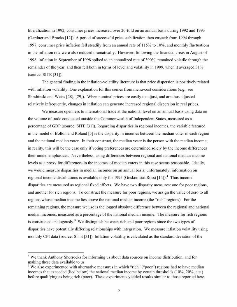
region may be correlated across time periods. To assess this possibility, we present in Table 3 estimates

obtained using a random-effects panel specification. The estimates we obtain are very close relative to

their counterparts in Table 2, both in terms of quantitative and statistical significance. For example, the

coefficient on trade openness is –2.778 in this case (with standard deviation 0.794), in comparison with

the estimates (-2.299, 0.695) reported in Table 2. The biggest difference in results we obtain is in terms

of estimated standard errors, which are systematically higher in this case, but not by much. Indeed, in

only one case would this matter under a Classical hypothesis-testing exercise: the p value associated with

the coefficient on low-median income moves from 0.084 under the Table 2 estimates, to 0.125 in this

case. Thus potential problems arising from correlated regional errors seem minor.

14

In considering these results, it is important to be mindful of the fact that we do not observe

economic integration directly. Rather, the results are based on the measure of integration generated by

the statistical model of commodity trade outlined in Section II. This raises the possibility that the results

are tainted by inconsistency arising from potential mis-measurement. In an effort to quantify the extent of

potential mis-measurement, and to evaluate the potential influence of mis-measurement on these results,

we obtained a second set of estimates using the mis-measurement model developed by Hausman,

Abrevaya, and Scott-Morton [18]. The model is a modification of the probit model (2) that incorporates

two additional components. Recall that yi(s) denotes our measure of whether region i is integrated in year

s. Letting y*i(s) denote the corresponding actual integration status of region i in year s, the additional

components are given by

(3) α0 = Pr(yi(s) = 1| y*i(s) = 0) ,

(4) α1 = Pr(yi(s) = 0| y*i(s) = 1).

Thus α0 denotes the probability that region i is spuriously classified as being integrated in period s, and α1

denotes the probability that the region is spuriously classified as not being integrated. Taking into

account these probabilities of mis-measurement, (2) becomes

(5) )B)s(X()1()1)s(y(prob i100i Φα−α−+α== .

We estimated this model using non-linear least squares, which involves minimizing

(6) ( )∑ =− 2ii 1)s(y(prob)s(y

over (α0 α1 B); estimates are presented in Table 4. We were unable to obtain estimates of this model for

the full set of variables considered above, thus Table 4 presents results only for the restricted set of

variables used to generate the second set of results presented in Tables 2 and 3. Given the minimal

explanatory power of the excluded variables in the probit model, their exclusion in this mis-measurement

model seems warranted (indeed, their lack of explanatory power seems to be the source of the difficulties

in estimating the fully-specified model).

Comparing the results presented in Tables 2 and 4, problems associated with mis-measurement

seem minor in this application. First, note that the estimated value of α0 (0.003, or 0.3%) is small and

statistically insignificant. In contrast, the estimated value of α1 is non-trivial (6.9%) and statistically

15

significant at the 5% level, indicating that our integration measure tends to understate the true extent of

economic integration in Russia. However, this carries only minor implications for the additional

coefficient estimates. In particular, the estimated signs of each coefficient are the same in both models.

Also, the pattern of statistical significance across variables is the same in both tables, with one exception:

the coefficient on high median income was insignificant in the probit model, but is significant at the 10%

level in the mis-specification model. Finally, quantitative significance measures are somewhat lower in

the mis-specification model (again, with high median income serving as the exception), but remain

substantial. For example, a one-standard-deviation increase in the trade-openness variable corresponds

with a 5.5 percentage point decrease in the estimated probability of being integrated in this case, as

compared with a 7.2 percentage point decrease in the probit model. In sum, although we are only able to

measure regional patterns of economic integration rather than observe these patterns directly, associated

problems arising from potential mis-measurement do not seem to be a serious concern in this application.

We conclude with a note regarding the 0-1 measure we use to characterize regional integration.

Recall how this measure is constructed: region i is deemed to be integrated in period s (and thus yi(s) is

set to 1) if its coefficient on logged distance is estimated as positive and statistically significant in

regression model (1); otherwise yi(s) is set to 0. Among the attractive features of this approach is the

straightforward means in which the measure may be aggregated over regions to achieve a dynamic

characterization of the extent of integration at the national level, e.g., as is done in Figure 1. However,

the conversion of a continuous measure of the importance of distance in accounting for regional patterns

of price dispersion into a 0-1 measure imposes a certain loss of informational content. Our own view is

that this imposition is appropriate: region A should not necessarily be deemed to be twice as strongly

integrated with its domestic trading partners than region B just because A’s standardized distance

coefficient is twice a large as B’s. Nevertheless, the robustness of the inferences based on our 0-1

measure is an important consideration; thus an exploration of the impact of this imposition seems

worthwhile.

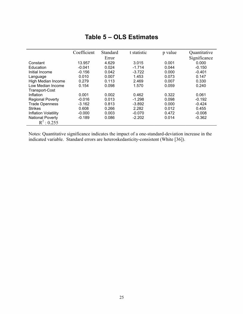
To do this, we respecified yi(s) as the standardized distance coefficient (i.e., the t statistic of the

distance coefficient) estimated in (1). We then estimated the relationship between this alternative

measure of integration and our explanatory variables using OLS; results are given in Table 5. Several

features of these results mirror those obtained using the 0-1 measure. Notably, the negative and

statistically significant relationship observed between integration and openness to international trade is

evident once again; the same is true for the regional measures of educational attainment and initial

incomes, and the national measure of poverty. Also evident once again is the weak statistical link

between integration and inflation volatility; indeed, the link is much weaker in this case.

16

The biggest difference in results involves the low-median-income measure, whose coefficient is

positive and significant in this case. This is perhaps due to a second difference in results, this time

involving the regional poverty measure. Previously, the coefficient on this variable was essentially zero;

in this case it is negative and significant. Thus the results based on the 0-1 measure suggest that sub-par

median regional incomes pose the greatest relative threat to regional integration, while the results in this

case suggest that the incidence of regional poverty poses the greatest relative threat. In either case, there

is an evident link in the data between regional economic stagnation and a weakening of economic

integration. Again, this is the relationship one would expect in light of the Bolton-Roland model.

As a final comparison, statistical links between the explanatory variables and this alternative

measure of integration are generally stronger than was the case with the 0-1 measure, with transport-cost

inflation and inflation volatility providing the exceptions. Thus there does appear to be some

deterioration in informational content associated with the use of the 0-1 measure. However, the

deterioration is relatively minor, as are differences in the general characterizations of integration that

emerge from the use of either measure.

V. Conclusions

The purpose of this paper has been to use the case of Russia in order to better understand forces

that may be responsible for undermining economic and political integration in post-socialist countries. In

order to quantify integration dynamics we have used a statistical model of commodity trade. To account

for these dynamics we have relied on guidance from theoretical work that highlights the potentially

destabilizing impact on economic and political integration of openness to international trade, regional

income disparities and inflation volatility.

Our analysis has produced four main findings. First, at the aggregate level, Russia has

experienced substantial fluctuations in the share of internally integrated regions. Specifically, following

an initial period of widespread integration in 1995, Russia gradually became fragmented in 1996 and

1997, and then became re-integrated by 1998. Underlying this aggregate behavior is a considerable

degree of diversity in the specific integration patterns observed across regions.

Second, openness to international trade seems to have worked to undermine Russia’s internal

economic coherence. This result provides an important caveat to the standard policy prescription that

trade liberalization is critical because it forces enterprises to restructure and allows regions to reap gains

from trade. Our results suggest that regions within Russia have actively substituted between domestic

and international trading partners in the latter half of the 1900s. This result complements Young’s [39]

observation that China’s internal market became more fragmented during a period when China expanded

its trade on world markets.

17

Third, striking disparities in regional incomes also seem to have undermined integration within

Russia. This is most clearly evident among relatively poor regions, although it is also the case that

regions with relatively high initial incomes on average exhibit lower propensities towards internal

integration. This seemingly presents federal policymakers interested in preserving national unity with a

difficult policy challenge: address the plight of relatively poor regions without imposing a politically

unacceptable burden in doing so on relatively rich regions.

Finally, the period of high inflation volatility associated with the financial crisis does seem to

have had an impact on internal integration within Russia, but substantially less than what one might

expect given the severity of the episode.

We recognize that several of the theories noted above specifically address the issue of political

integration, while our focus is on economic integration. Nevertheless, we believe these theories are of

potential relevance in this context, due to natural links between economic and political integration. For

example, external trade coalitions arising from trade-liberalization reforms do not merely afford regions

with the opportunity to self-finance regional public-good provision; they also provide regions with the

option of pursuing trade relationships with regions outside their own country, potentially lessening the

importance of internal trading partners. Thus if trade liberalization was in fact actively working to

produce political disintegration within a country, we might well expect to observe economic

disintegration (in the guise of a decreased importance of domestic trading partners) in parallel, or even as

a symptom of political disintegration that becomes apparent well in advance of an actual breakup. As

noted in Section II, in the case of Russia, we find empirical support for this link. Specifically, we find a

strong negative association between our measure of economic integration and Treisman’s [34] measure of

regional tax withholdings to the federal government, which serves as a useful measure of political

disintegration.

18

References 1. A. Alesina, E. Spoloare, and R. Wacziarg, Economic integration and political disintegration,

American Economic Review 90 (2000) 1276-1296. 2. D. Berkowitz and D.N. DeJong, Russia’s internal border, Regional Science and Urban Economics 29 (1999) 633-649. 3. ___________, The evolution of market integration in Russia, Economics of Transition 9 (2001)

87-104. 4. ______________, Policy reform and growth in post-soviet Russia, European Economic Review

47 (2003) 141-156. 5. P. Bolton and G. Roland, The breakup of nations: a political economy analysis, Quarterly Journal

of Economics 112 (1997) 1057-1090. 6. A. Casella, The role of market size in the formation of jurisdictions, Review of Economic Studies

68 (2001) 83-108. 7. P. De Masi and V. Koen, Relative price convergence in Russia. IMF Staff Papers 43 (1996) 97-

122. 8. G. Debelle and O. Lamont, Relative price variability and inflation: evidence from U.S.

cities, Journal of Political Economy 105 (1997) 132-152. 9. C. Engel and J.H. Rogers, How wide is the border? American Economic Review 86 (1996) 1112-

1125. 10. R.E. Ericson, Does Russia have a “market economy”? East European Politics and Society 15

(2001) 291-309. 11. L. Freinkman, D. Treisman, and S. Titov, Subnational budgeting in Russia, World Bank

Technical Paper No. 452, Washington D.C., 1999. 12. B. Gardner and K. Brooks, Food prices and market integration in Russia: 1992-93, American

Journal of Agricultural Economics 76 (1994) 641-646. 13. Goskomstat Rossii, Obrazovanie Nasilenie Rossii (po dannim mikroperepisi nasileniya

1994 g.). Goskomstat Rossii, Moscow, 1995a. 14. _____________ Raspredelenie naseleniia Rossii po vladeniiu iazykami ( po dannym

mikroperepisi naseleniia 1994 g.). Goskomstat Rossii, Moscow, 1995b. 15. _________, Rossiiskiy Statisticheskiy Yezhegodnik. Moskva: Goskomstat Rossii. 1996, 2000c. 16. _________, Regiony Rossii. Moskva: Goskomstat Rossii. 2000a. 17. __________, Sotsial’noye ekonomicheskoye polozheniye v Rossii, Moskva: Goskomstat Rossii.

2000b.

19

18. J. Hausman, J. Abrevaya, and F.M. Scott-Morton, Misclassification of the dependent variable in a

discrete-response setting, Journal of Econometrics 87 (1998) 239-269. 19. J. Konienczny and A. Skrzypacz, The behavior of price dispersion in a natural experiment,

Stanford Graduate School of Business Research Paper No.1641, July 2000. 20. P. Krugman, Increasing returns and economic geography, Journal of Political Economy 99 (1991)

483-499. 21. S. Lach, and D. Tsiddon, The behavior of prices and inflation: an empirical analysis of

disaggregated price data, Journal of Political Economy 100 (1992) 349-398. 22. B. Mitchneck, An assessment of the growing local economic development

function of local authorities in Russia, Economic Geography 71 (1995) 150-170. 23. OECD, Economic survey: the Russian federation, Paris, OECD, 1997. 24. OECD, Economic survey: the Russian federation, Paris, OECD, 2000. 25. D.C. Parsley, Inflation and relative price variability in the short and long run: new

evidence from the United States, Journal of Money, Credit and Banking, 28 (1996) 323-341. 26. D. Parsley and S.J. Wei, Convergence to the law of one price without trade barriers or currency

fluctuations, Quarterly Journal of Economics November 111 (1996) 1211-1236. 27. E. Serova, Federal agro-food policy in the conditions of the financial and economic crisis,

Russian Economy November 1998. 28. E. Sheshinski and Y. Weiss, Inflation and costs of price adjustment, Review of Economic

Studies 44 (1977) 287-303. 29. ________________________, Optimum pricing policy under stochastic inflation, Review of

Economic Studies 50 (1983) 513-529. 30. M. Silver and C. Ionnidis, Inter country differences in the relationship between relative

price variability and average prices, Journal of Political Economy 109 (2001) 335-374. 31. SITE (Stockholm Institute for Transition Economics), Russian Economic Trends, database

available online at http://www.hhs.se/site/ret/exceldb/default.htm, 2000. 32. D.S. Treisman, Russia’s ethnic revival: the separatist activism of regional leaders in a post-

communist order, World Politics, January 1997. 33. D.S. Treisman, After the deluge: regional crises and political consolidation in Russia, University

of Michigan Press, Ann Arbor 1999a. 34. D.S. Treisman, Russia’s tax crisis: explaining falling revenues in a transitional economy,

Economics and Politics 11 (1999b) 145-170. 35. T. Van Hoomissen, Price dispersion and inflation: evidence from Israel, Journal of Political

20

Economy 96 (1988) 1303-1314. 36. H. White, A heteroskedasticity-consistent covariance matrix estimator and a direct test for

heteroskedasticity, Econometrica 48 (1980) 817-838. 37. A. Young, The razor's edge: distortions and incremental reform in the People's Republic of China,

Quarterly Journal of Economics 115 (2001) 1091-1135.

21

Table 1 – Description of Variables

Variable Type: National, Time-Varying Trade Openness: Trade volume (exports plus imports) as a percentage of GDP Strikes: Workdays lost in strikes per thousand workers Inflation Volatility: Standard deviation of monthly inflation rate observed during each

year National Poverty: Percentage of population living below the official poverty line

Variable Type: Regional, Fixed

Education: Percentage of population 15 years or older as of 1994 that completed high school and received some post-secondary education

Initial Income: Ratio of money income per capita to the cost of a basket of basic

food goods, 1993, fourth quarter Language: Percentage of people in 1994 that do not consider Russian as their

native language High Median Income: Zero if median income lies below national median income; logged

absolute difference between regional and national median incomes (as a percentage of national median income) otherwise

Low Median Income: Zero if median income lies above national median income; logged

absolute difference between regional and national median incomes (as a percentage of national median income) otherwise

Variable Type: Regional, Time-Varying

Transport-Cost Inflation: Annual regional inflation rate in freight transport costs Regional Poverty: Percentage of regional population living below the official poverty

line

22

Table 2 – Probit Estimates

Coefficient Standard Error

t statistic p value Quantitative Significance

Constant 12.515 4.415 2.830 0.005 0.0% Education -0.064 0.024 -2.620 0.009 -5.4% Initial Income -0.102 0.040 -2.580 0.010 -6.2% Language 0.007 0.006 1.040 0.298 2.4% High Median Income 0.164 0.130 1.250 0.210 4.5% Low Median Income -0.133 0.107 -1.240 0.215 -4.8% Transport-Cost Inflation 0.002 0.002 0.950 0.344 3.1% Regional Poverty -0.008 0.011 -0.690 0.488 -2.1% Trade Openness -2.054 0.761 -2.700 0.007 -6.4% Strikes 0.206 0.265 0.780 0.437 3.6% Inflation Volatility -0.005 0.003 -1.440 0.149 -4.1% National Poverty -0.214 0.082 -2.620 0.009 -9.6%

-2*ln(L): 290.067

Coefficient Standard Error

t statistic p value Quantitative Significance

Constant 15.058 2.524 5.970 0.000 0.0% Education -0.066 0.024 -2.750 0.006 -5.6% Initial Income -0.092 0.038 -2.410 0.016 -5.6% Language -- -- -- -- -- High Median Income 0.150 0.126 1.190 0.234 4.2% Low Median Income -0.149 0.086 -1.730 0.084 -5.5% Transport-Cost Inflation -- -- -- -- -- Regional Poverty -- -- -- -- -- Trade Openness -2.299 0.695 -3.310 0.001 -7.2% Strikes -- -- -- -- -- Inflation Volatility -0.004 0.003 -1.250 0.212 -3.5% National Poverty -0.253 0.053 -4.820 0.000 -11.4%

-2*ln(L): 292.400

Notes: Quantitative significance indicates the impact on the probability of a region being defined as economically integrated of a one-standard-deviation increase in the indicated variable. Regarding fit, count R2 statistics are 0.83 in both cases. The exclusion of Language, Transport-Cost Inflation, Regional Poverty and Strikes from the model yields a likelihood ratio statistic of 2.33, which has a p value of 0.67.

23

Table 3 – Random Effects Probit Estimates

Coefficient Standard Error

t statistic p value Quantitative Significance

Constant 18.477 3.147 5.87 0.000 0.0% Education -0.079 0.037 -2.15 0.031 -5.2% Initial Income -0.117 0.059 -1.99 0.046 -5.5% High-Median Income 0.162 0.184 0.88 0.378 3.5% Low-Median Income -0.200 0.131 -1.53 0.125 -5.7% Trade Openness -2.778 0.794 -3.50 0.000 -6.8% Inflation Volatility -0.005 0.004 -1.39 0.163 -3.4% National Poverty -0.313 0.063 -4.97 0.000 -10.9% -2*ln(L): 281.06

24

Table 4 – Misclassification Model

Coefficient Standard Error

t statistic p value Quantitative Significance

Pr(y=1|y*=0) 0.003 0.561 0.006 0.498 -- Pr(y=0|y*=1) 0.069 0.039 1.752 0.040 -- Constant 23.873 12.806 1.864 0.031 0.0% Education -0.121 0.079 -1.53 0.063 -4.3% Initial Income -0.168 0.112 -1.505 0.066 -4.2% High Median Income 0.503 0.361 1.394 0.082 5.8% Low Median Income -0.207 0.166 -1.248 0.106 -3.2% Trade Openness -4.197 2.732 -1.536 0.062 -5.5% Inflation Volatility -0.006 0.007 -0.761 0.223 -2.0% National Poverty -0.333 0.183 -1.818 0.035 -6.2%

Notes: Pr(y=1|y*=0) indicates the probability of a non-integrated region being misclassified as an integrated region, and Pr(y=0|y*=1) indicates the probability of an integrated region being misclassified as a non-integrated region.

25

Table 5 – OLS Estimates

Coefficient Standard Error

t statistic p value Quantitative Significance

Constant 13.957 4.629 3.015 0.001 0.000 Education -0.041 0.024 -1.714 0.044 -0.150 Initial Income -0.156 0.042 -3.722 0.000 -0.401 Language 0.010 0.007 1.453 0.073 0.147 High Median Income 0.279 0.113 2.469 0.007 0.330 Low Median Income 0.154 0.098 1.570 0.059 0.240 Transport-Cost Inflation 0.001 0.002 0.462 0.322 0.061 Regional Poverty -0.016 0.013 -1.298 0.098 -0.192 Trade Openness -3.162 0.813 -3.892 0.000 -0.424 Strikes 0.608 0.266 2.282 0.012 0.455 Inflation Volatility -0.000 0.003 -0.070 0.472 -0.008 National Poverty -0.189 0.086 -2.202 0.014 -0.362

R2 : 0.255

Notes: Quantitative significance indicates the impact of a one-standard-deviation increase in the indicated variable. Standard errors are heteroskedasticity-consistent (White [36]).

26