regional-scale mapping of groundwater discharge zones ... · the belly river group subcrops in the...

HYDROLOGICAL PROCESSESHydrol. Process. 28, 5662–5673 (2014)Published online 5 October 2013 in Wiley Online Library(wileyonlinelibrary.com) DOI: 10.1002/hyp.10068

Regional-scale mapping of groundwater discharge zones usingthermal satellite imagery

G. Z. Sass,1 I. F. Creed,1* J. Riddell2 and S. E. Bayley31 Department of Biology, Western University, London, ON, N6A 5B7, Canada

2 Energy Resources Conservation Board, Alberta Geological Survey, Edmonton, AB T6B 2X3, Canada3 Department of Biological Sciences, University of Alberta, Edmonton, AB T6G 2E9, Canada

*CUniE-m

Cop

Abstract:

Mapping groundwater discharge zones at broad spatial scales remains a challenge, particularly in data sparse regions. We applieda regional scale mapping approach based on thermal remote sensing to map discharge zones in a complex watershed with a broaddiversity of geological materials, land cover and topographic variation situated within the Prairie Parkland of northern Alberta,Canada. We acquired winter thermal imagery from the USGS Landsat archive to demonstrate the utility of this data source forapplications that can complement both scientific and management programs. We showed that the thermally determined potentialdischarge areas were corroborated with hydrological (spring locations) and chemical (conservative tracers of groundwater) data.This study demonstrates how thermal remote sensing can form part of a comprehensive mapping framework to investigategroundwater resources over broad spatial scales. Copyright © 2013 John Wiley & Sons, Ltd.

KEY WORDS groundwater; discharge; mapping; Landsat; thermal; remote sensing; Prairie Pothole

Received 8 February 2013; Accepted 11 September 2013

INTRODUCTION

Discharge water is found where groundwater flowsupwards towards the land surface or where the watertable intersects the land surface. A conceptual delineationof discharge vs recharge zones was developed in detail bythe seminal work of József Tóth in the rolling glaciatedterrain of Alberta, Canada (Tóth, 1963, 1971). Accordingto his description, the groundwater regime reflects thecombined effects of topography and geology, whichtogether affect the distribution, motion, chemistry andtemperature of groundwater (Figure 1). Based on thisconceptual model, discharge zones are generally locatedin topographically low areas that receive groundwaterfrom regional, intermediate and local-scale flow systemsand where lakes, rivers or groundwater-fed wetlands oftenexist. Discharge can occur as point features, such assprings that focus discharge in small areas, or over broadareas, such as riparian areas and seepage faces.As a result of modified hydrological, biogeochemical and

thermal properties of discharge zones, knowledge of theirdistribution across watersheds and how they connect to thelarger hydrological system is essential for understandingecosystem processes (Brunke and Gonser, 1997) as well as

orrespondence to: Irena Creed, Department of Biology, Westernversity, London, ON N6A 5B7, Canada.ail: [email protected]

yright © 2013 John Wiley & Sons, Ltd.

improving freshwater management, regulation and gover-nance (Neufeld, 2000; O’Connor, 2002; Pires, 2004). Areasof active groundwater discharge have important implica-tions for hydrology, as they play an important role in thedynamics of variable source areas and therefore affect runoffprocesses (Winter et al., 1998). Groundwater discharge notonly influences water quantity by providing a steady sourceof water (baseflow) but it also may influence ecosystems byproviding a modified environment through its thermal andchemical signature. The temperature of groundwaterdischarge zones reflects that of ambient conditions: coolerin the summer and warmer in the winter (Cartwright, 1974).For example, in summer time, groundwater dischargeentering streams and lakes provides a cooler environmentand thus favour coldwater fish like trout (Curry andNoakes,1995; Power et al., 1999). Discharging groundwater alsohas a chemical signature that reflects the flowpaths it hastraversed often translating to water that has high concentra-tions of total dissolved solids (TDS), a degree ofmineralization proportional to the time the water has spentin the ground (Batelaan et al., 2003; Soulsby et al., 2009). Interms of management, knowing where groundwaterdischarges onto the surface is important as it contributesto an understanding of the entire flow system which isespecially useful to track the movement of contaminants(Whiteman et al., 2012). To meet these scientific andmanagement needs, conceptual and applied approaches are

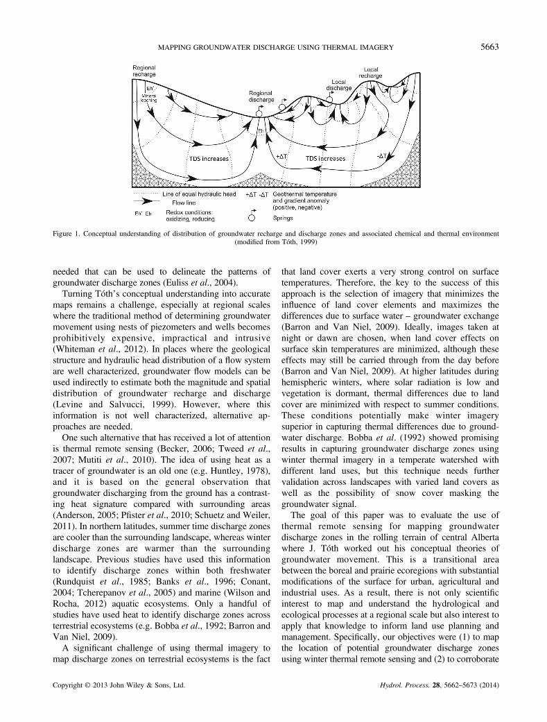
Figure 1. Conceptual understanding of distribution of groundwater recharge and discharge zones and associated chemical and thermal environment(modified from Tóth, 1999)

5663MAPPING GROUNDWATER DISCHARGE USING THERMAL IMAGERY

needed that can be used to delineate the patterns ofgroundwater discharge zones (Euliss et al., 2004).Turning Tóth’s conceptual understanding into accurate

maps remains a challenge, especially at regional scaleswhere the traditional method of determining groundwatermovement using nests of piezometers and wells becomesprohibitively expensive, impractical and intrusive(Whiteman et al., 2012). In places where the geologicalstructure and hydraulic head distribution of a flow systemare well characterized, groundwater flow models can beused indirectly to estimate both the magnitude and spatialdistribution of groundwater recharge and discharge(Levine and Salvucci, 1999). However, where thisinformation is not well characterized, alternative ap-proaches are needed.One such alternative that has received a lot of attention

is thermal remote sensing (Becker, 2006; Tweed et al.,2007; Mutiti et al., 2010). The idea of using heat as atracer of groundwater is an old one (e.g. Huntley, 1978),and it is based on the general observation thatgroundwater discharging from the ground has a contrast-ing heat signature compared with surrounding areas(Anderson, 2005; Pfister et al., 2010; Schuetz and Weiler,2011). In northern latitudes, summer time discharge zonesare cooler than the surrounding landscape, whereas winterdischarge zones are warmer than the surroundinglandscape. Previous studies have used this informationto identify discharge zones within both freshwater(Rundquist et al., 1985; Banks et al., 1996; Conant,2004; Tcherepanov et al., 2005) and marine (Wilson andRocha, 2012) aquatic ecosystems. Only a handful ofstudies have used heat to identify discharge zones acrossterrestrial ecosystems (e.g. Bobba et al., 1992; Barron andVan Niel, 2009).A significant challenge of using thermal imagery to

map discharge zones on terrestrial ecosystems is the fact

Copyright © 2013 John Wiley & Sons, Ltd.

that land cover exerts a very strong control on surfacetemperatures. Therefore, the key to the success of thisapproach is the selection of imagery that minimizes theinfluence of land cover elements and maximizes thedifferences due to surface water – groundwater exchange(Barron and Van Niel, 2009). Ideally, images taken atnight or dawn are chosen, when land cover effects onsurface skin temperatures are minimized, although theseeffects may still be carried through from the day before(Barron and Van Niel, 2009). At higher latitudes duringhemispheric winters, where solar radiation is low andvegetation is dormant, thermal differences due to landcover are minimized with respect to summer conditions.These conditions potentially make winter imagerysuperior in capturing thermal differences due to ground-water discharge. Bobba et al. (1992) showed promisingresults in capturing groundwater discharge zones usingwinter thermal imagery in a temperate watershed withdifferent land uses, but this technique needs furthervalidation across landscapes with varied land covers aswell as the possibility of snow cover masking thegroundwater signal.The goal of this paper was to evaluate the use of

thermal remote sensing for mapping groundwaterdischarge zones in the rolling terrain of central Albertawhere J. Tóth worked out his conceptual theories ofgroundwater movement. This is a transitional areabetween the boreal and prairie ecoregions with substantialmodifications of the surface for urban, agricultural andindustrial uses. As a result, there is not only scientificinterest to map and understand the hydrological andecological processes at a regional scale but also interest toapply that knowledge to inform land use planning andmanagement. Specifically, our objectives were (1) to mapthe location of potential groundwater discharge zonesusing winter thermal remote sensing and (2) to corroborate

Hydrol. Process. 28, 5662–5673 (2014)

5664 G. Z. SASS ET AL.

these maps using ground-based hydrological andchemical datasets. Our remote sensing methodology isbased on the assumption that discharging groundwaterhas a thermal signature that is distinct from non-discharge areas; that is, in winter, the ground surfacein discharge areas is relatively warmer than surroundingnon-discharge areas because of the moderating effect ofupwelling groundwater.

METHODOLOGY

Study region

The study region is the Beaverhill subwatershed inAlberta (53.5°N, 113°W) centred on the Cooking Lakemoraine located 50 km east of Edmonton and occupying atotal area of 4405 km2 (Figure 2A). The Beaverhillsubwatershed contains Beaverhill Lake, an aquatic systeminternationally recognized for its shorebirds and water-fowl (RAMSAR convention of 1971) that drains into theNorth Saskatchewan River. Most of the Cooking Lakemoraine is designated as part of national (Elk IslandNational Park) and provincial (Cooking Lake-BlackfootGrazing, Wildlife, Provincial Recreation Area, theMinistik Bird Sanctuary, and Miquelon Lake ProvincialPark) protected areas. The rest of the Beaverhillsubwatershed comprises agricultural land farmed eitheras cropland or pastureland or is undergoing residential(e.g. Edmonton and Fort Saskatchewan) and industrialdevelopment (e.g. upgraders and refineries).Bedrock geology is characterized by three major bedrock

units including the Horseshoe Canyon Formation, theBearpaw Formation and the Belly River Group (Figure 3A,Hamilton et al., 1998). The Horseshoe Canyon Formationunderlies the glacial materials over the majority of the study

Figure 2. Maps of the Beaverhills subwatershed study region: (A) general locof climate and hydrological measurement lo


region. It was deposited in a marginal marine setting and iscomposed of fine tomedium grained sediments occurring aslenticular, inter-fingered within muddy, transgressivesediments (Stein, 1979). The Bearpaw Formation consistsof marine shale, with bentonite, silty shale, and discontin-uous sandstone beds where it inter-fingers with theoverlying Horseshoe Canyon Formation. The BearpawFormation’s subcrop area cuts across the middle of thewatershed along the eastern edge of the Cooking Lakemoraine. The Belly River Group subcrops in the easternportion of the study region and is composed also of largelymarginal-marine sediments with localized areas of coarse-grained fluvial sand deposits.The last glaciation left as many as three till sequences

with variable thickness (average thickness of 21m). Theglacial till is vertically interspersed with sand and gravellenses of glacio-fluvial origin as well as glacio-lacustrinelakebeds (Figure 3B, Hamilton et al., 1998). The surficialdeposits are notably thicker within the Beaverhillsubwatershed than the surrounding Prairie as a result ofthe presence of the moraine (Barker et al., 2011). Closerto the North Saskatchewan River in the north, there aresizable deposits of sand and gravel of fluvial origin.Topography reflects glacial depositional processes and

consists of hummocky, knob and kettle formations of themoraine at higher elevations surrounded by flat to rollinglandscapes at lower elevations surrounding the moraine(Figure 3C). Topographic relief ranges from a high of812m in the moraine to a low of 586m along the NorthSaskatchewan River. The soils that have formed on theseglacial and fluvial deposits are mainly Orthic GrayLuvisols and Black Chernozemics.A mixed-wood boreal forest characterizes the natural

vegetation cover of the region, with prairie transitionspecies including tree species of trembling aspen

ation and main administrative and physiographic features and (B) locationscations (groundwater springs and wells)

Hydrol. Process. 28, 5662–5673 (2014)

Figure 3. (A) Bedrock geology (adapted from Alberta Geological Survey Map 236, Hamilton et al., 1998), (B) surficial geology (adapted from AlbertaGeological Survey Map 236, Hamilton et al., 1998), (C) elevation and (D) land use of the Beaverhills subwatershed. The red line depicts the outline of

the Cooking Lake moraine


(Populus tremuloides Michx.), balsam poplar (Populusbalsamifera L.) and white birch (Betula papyriferaMarsh) (Strong and Leggat, 1981) interspersed withgrassland (Figure 3D). The lands outside of the protectedareas have been farmed since the early 1900s andcomprise croplands (e.g. barley, oats and canola) andpasturelands.The climate is continental with cold winters and warm

summers. Based on a 30-year (1971–2000) climate normalfor Edmonton International Airport (Environment CanadaClimate Normals [http://www.climate.weatheroffice.gc.ca/climate_normals/index_e.html]), average January and Julytemperatures are �13.5 and 15.9 °C, respectively. Annualprecipitation is 483mm, most of it (~70%) falling as rainbetween the months of May and September. Evaporativedemand is highest during this time of year (450mm ofpotential evapotranspiration [May–September]) resulting inlittle water left over for surface runoff. Although small as apercentage of the overall budget (~20%), winter precipitation


(mostly as snow) can be an important contributor of localrunoff into wetlands as the snow melts in the spring.In terms of the surface energy balance, solar radiation

reaches a minimum around the December solstice(Figure 4). This minimum in energy input by the sun isreflected in soil temperatures that reach their minimumconcurrently or sometime after the solar minimumdepending on the depth of measurement. Soil tempera-ture, measured 5 cm belowground, is correlated linearlywith air temperature until the snowpack forms, whensoil temperatures are decoupled from the atmosphere(Figure 5). In most years, the snowpack forms by middleof December and lasts until March except for occasionalmid-winter thaws (Figure 4).The depth and spatial extent of concrete soil frost are

highly variable in the study region and are highly dependenton antecedent soil moisture conditions prior to wintermonths, and the timing and nature of the snowpackaccumulation (Metcalfe and Buttle, 1999). Wet conditions

Hydrol. Process. 28, 5662–5673 (2014)

http://www.climate.weatheroffice.gc.ca/climate_normals/index_e.html

http://www.climate.weatheroffice.gc.ca/climate_normals/index_e.html

Figure 4. Two-year sequence of daily measurements in incoming solar radiation, soil temperature (5 cm below ground) and snow depth recorded atMundare climate station [http://agriculture.alberta.ca/acis/alberta-weather-data-viewer.jsp] located near the eastern boundary of Beaverhill subwatershed

(Figure 2B)

Figure 5. Coupling of air temperature with soil temperature as recorded atMundare climate station (same data series as in Figure 4): (A) all data and (B) level ofcorrelation for all air temperature measurements below the freezing mark and progressively discarding measurements with specific snow depth (i.e. at snowdepth of 20 cm all sub-zero data points are analysed, but at zero, snow depth only measurements when there was no snow accumulation were analysed)


followed by cold temperatures and little snowpack leads todeep soil frost development. In fact, soil frost can alsooccur in the spring given the slow warm-up and freezethaw cycles. However, even when conditions are optimalfor significant soil frost accumulation, it is uncommon forsoil frost to exceed 1m depth from the land surface(Löfvenius et al., 2003). Groundwater discharging tosurface melts soil frost from below prior to air temperaturedriven soil frost melting. This is particularly true for areaswithout concrete soil frost development as the soilmedia hasbeen shown to remain permeable facilitating infiltration andby extension upward exfiltration or discharge to surface(Redding and Devito, 2011).The climate, geology and topography have collectively

created a hydrological system dominated by numerousshallow lakes and wetlands on the surface and by localand regional aquifers below the surface. The relativelylow precipitation rate coupled with high evaporativedemand translates into minimal surface water flow


volumes with only a few intermittent or slow-movingstreams in the subwatershed. Precipitation patterns drivefluctuations in water levels in wetlands and lakes. Forexample, Beaverhill Lake has completely dried up on twooccasions in the past 100 years (1945 and 2009). Giventhe low permeability of the till and the protected statusof the moraine, there are many more lakes and wetlandson the moraine than on the surrounding agriculturalregions. Although the transmission rate of water intothe shallow and deeper geological deposits is slow, themoraine still serves as an important source ofgroundwater recharge in the area.Regional hydrogeological flow patterns are reasonably

well documented in the Beaverhill subwatershed. Theflow systems within the shallow intertill aquifers aredriven by local to intermediate-scale topographic featureson the moraine. The regional flow pattern in the bedrockaquifers is dominated by radial flow towards the flanks ofthe topographic high created by the Cooking Lake

Hydrol. Process. 28, 5662–5673 (2014)

http://agriculture.alberta.ca/acis/alberta-weather-data-viewer.jsp


moraine. Some of this water discharges in springs andseepages along the moraine’s edge, which is coincidentwith the edge of the Bearpaw Formation subcrop edge. Asa result, it has great potential to impede vertical flow (highpermeability contrast relative to the other bedrockformations and the overlying glacial materials) (Barkeret al., 2011). This creates what are known as contactsprings, which develop where sediments with relativelyhigh permeability rest directly on a geological body withlow permeability, such as clay or marine shale in the caseof the Bearpaw Formation. Downward flow from theHorseshoe Canyon to the Belly River is well documentedwith potentiometric data showing an upward gradientacross the Bearpaw Formation (Stein, 1979). Themajority of the recharge occurring on the moraine enterslocal and intermediate scale groundwater flow systems, asonly a small flux would be possible through the shale withlow permeability that constitutes the Bearpaw Formation.

Mapping groundwater discharge zones using thermal imagery

Criteria for image selection. A key aspect of ourmethodology was the selection of appropriate imagery tomap groundwater discharge zones. We used thermalimages acquired by the Landsat-5 Thematic Mapper (TM)(10.45–12.4 μm) and Landsat-7 Enhanced ThematicMapper (ETM) (10.31–12.36μm) sensors downloadedfrom the USGS Landsat archives (http://glovis.usgs.gov)to complete the mapping. As a pre-screening step, imageswere discarded if there were clouds or haze across thestudy region or if there were other image anomalies. Next,we applied the following biophysical image selectioncriteria to the entire archive of imagery available for thestudy region (1983–2011) in order to identify imagerywith the highest likelihood of reflecting spatial patterns ofgroundwater discharge.The challenge in using sun-synchronous Landsat thermal

imagery (local overpass times of about 11:30 AM) formapping discharge zones is that the spatial pattern of surfaceskin temperature (which the Landsat thermal sensormeasures) can be dominated by the spatial pattern in landcover each reflecting its own surface energy dynamics. Inorder to minimize the thermal signal of land cover, weselected imagery captured during the time of year whensolar radiation is at a minimum (20 November–20 January)(Figure 4). Vegetation cover is also at a minimum duringthis time exposing the ground surface in most of theagriculturally dominated study region.In addition to land cover, snow can alsomask the potential

groundwater discharge signal by acting as an insulatingblanket where the surface temperatures of the snowpack donot necessarily reflect the temperature of the soil. Therefore,we discarded any imagery where the snowpack wasgreater than 5 cm deep across the study region.We arrived


at this heuristic by identifying a natural break in thecoefficient of determination curve testing the correlationbetween air and soil temperatures of the winter months,progressively discarding data points as a function of snowdepth (Figure 5B).Using these criteria, three Landsat TM thermal images

were selected for further analysis (image dates: 14January 2002, 30 November 2002 and 1 January 2003).Although previous studies used only one image for theirmapping, we assumed that a more robust spatial pattern ofgroundwater discharge zones could be extracted if thethermal images were combined to average out the image-to-image variability in hydrological conditions as wellsome of the thermal signal that comes from land and snowcover effects.

Image pre-processing. We checked geometric alignmentof the images by overlaying georeferenced hydrography androad layers and found all images to be well aligned acrossthe study region. Next, we converted digital numbersrecorded in the thermal images first to top-of-atmosphere(Equation 1) and then to at-sensor temperature usingcalibration constants (Equation 2) (Markham and Barker,1986; Barsi et al., 2003).

Lcal ¼ Gain*Qcal þ Offset (1)

where Lcal is calibrated radiance in W/(m2·sr·μm) Gain((W/(m2 · sr · μm))/counts) and Offset (W/(m2·sr·μm)) arerescaling factors provided in Landsat image metadata,and Qcal is the digital number of the thermal image.

T ¼ K2= ln K1=Lcal þ 1ð Þ½ � (2)

where T is effective at-sensor temperature in K assumingemissivity of one; K2 is calibration constant 2 in units ofK; K1 is calibration constant 1 in units of W/(m2·sr·μm);and Lcal is calibrated radiance in units of W/(m2∙sr∙μm).We used the values of 607.76 and 1260.56 for K1 and K2,respectively (Markham and Barker, 1986). At-sensortemperatures were converted from units of K to °C.Each image was captured under stable atmospheric

conditions. For this reason, we assumed that atmosphericeffects were uniform. Further, we assumed that surfaceeffects were spatially uniform and that conversion toabsolute surface temperatures was not necessary, as thefocus of the study was on extracting and analysing thespatial pattern of surface temperature. As a check, wecompared average at-sensor temperature (across the studyregion) and average hourly air temperature at all climatestations within the study region at the time of acquisitionand found a near one-to-one relationship (Figure 6).

Discharge zone mapping. The three images werecombined into one thermal map by computing an average

Hydrol. Process. 28, 5662–5673 (2014)

http://glovis.usgs.gov

Figure 6. The relationship between air temperature as measured byweather stations (Figure 2B) and at-sensor temperature measured by

satellite. The dashed line represents a 1 : 1 relationship

Figure 7. Thermal composite maps (A) based on an average, (B) standarddeviation and (C) coefficient of variation of three winter Landsat thermalimages. Areas of brown hues in map (A) are warmer areas potentially

corresponding to groundwater discharge zones


at-sensor temperature (Figure 7A). We masked out urbanareas, given the strong effect of the urban heat island,as well as open water areas, due to the different thermalsignature of ice (or open water) compared with landtemperatures. The temperature range in this combinedthermal map was �12.2 to �1.9 °C with a mean of�6.2 °C and standard deviation of 1.4 °C. We alsocomputed the standard deviation and coefficient ofvariation of each pixel of the three images to identifyareas that changed the most between the three images(Figure 7B and 6C).Next, we developed a simple 2-class classification

scheme to classify the thermal map into discharge andnon-discharge zones. A known area of strong dischargewas selected based on local accounts of springs andseepages as well as the general location of headwater areaof streams based on a hydrography layer. Image values ofthe averaged thermal map along a transect were digitallyextracted from a topographic high in the moraine tostretch across the potential discharge area and beyond(Figure 8A, B). A threshold between discharge and non-discharge classes was identified by looking for abruptchanges in temperature along a part of the transect withsimilar topography and land cover. Closer to the northernend of the transect, the temperature changes significantly(Δ3 °C) over a 3-km stretch of flat, agricultural terrain;the mid-point of this large temperature gradient was usedas the classification threshold between discharge and non-discharge areas (Figure 8C). After applying the selectedthreshold to the averaged thermal image, a 3 × 3 majorityfilter was used to smooth the classified image. Hereafter,we refer to the remote sensing derived classifieddischarge/non-discharge map as the classified dischargemap (Figure 7A).

Copyright © 2013 John Wiley & Sons, Ltd. Hydrol. Process. 28, 5662–5673 (2014)

Figure 8. Visual depiction of the method for selecting class boundary ofdischarge and non-discharge zones from the thermal composite map: (A) across-section was identified based on local knowledge of springs, (B) thecross-sectional profile of temperature wasmapped along the selected path and(C) an area of abrupt change in temperature was selected (red box in A)


Corroboration of ground-based and remotely senseddischarge map

Hydrological evidence: spring locations and water tabledepth. We used two hydrological sources of corroboratingevidence to assess the accuracy of the classified dischargemap: (1) spring locations mapped by the Alberta GeologicalSurvey (AGS) (http://www.ags.gov.ab.ca/publications/abstracts/DIG_2009_0002.html) and (2) static water-level


depth measured in shallow wells (<10m bgs [belowground surface]) extracted from the Alberta Water WellInformation Database (AWWID; http://environment.alberta.ca/01314.html) (Figure 2B). It was assumedthat the static water levels of shallow wells wouldreflect the position of the water table. The presence/absence of springs within the two zones (discharge andnon-discharge) was determined; the expectation wasthat all springs would fall within discharge zones. Thestatistically significant difference in at-sensor temperaturesbetween spring influenced areas (120m buffer aroundspring locations) and non-spring influenced areas wereassessed. Using the static water levels, non-parametricMann–Whitney U Tests were conducted to test thehypothesis that there were statistically significant (p< 0.05)differences in water-table depth between discharge andnon-discharge zones; we predicted that discharge zoneswould have shallower (i.e. closer to the ground surface)water tables.

Chemical evidence: water-well chemistry. All availablechemistry data measured in shallow wells (<10mbgs)from the AWWID were used to test for differences inoften used tracers of groundwater flow including theconcentrations of TDS, sodium (Na), chloride (Cl),calcium (Ca), and magnesium (Mg) as well as electricalconductivity (EC). Non-parametric Mann–Whitney UTests were conducted to test the hypothesis that therewere statistically significant (p< 0.05) differences inchemical signatures between discharge and non-dischargezones; we predicted that discharge zones would havehigher concentrations of these tracers than non-dischargezones reflecting a longer contact period with the substrate(Devito et al., 2000).

RESULTS

The thermally classified map of groundwater dischargezones is presented in Figure 9. Discharge zones occurredin topographically low areas but not necessarily thelowest areas. Discharge zones were located on the slopesand at the bottom of the slopes surrounding the moraine,especially the northeastern flank of the moraine and thearea surrounding the southwestern tip of Beaverhill Lake.Hydrological data provided independent support for the

thermally classified discharge map. Of the 26 springslocated within the non-urban portion of the Beaverhillsubwatershed according to the AGS-springs database, 22springs fell within the classified discharge zones,corresponding to an 85% accuracy of predicting springsas part of discharge zones. One other spring was locatedwithin 200m of the classified map boundary. Comparisonof averaged at-sensor temperatures (Figure 9 inset)

Hydrol. Process. 28, 5662–5673 (2014)

http://environment.alberta.ca/01314.html

http://environment.alberta.ca/01314.html

Figure 9. Classified groundwater discharge map inferred from satellitethermal remote sensing and conceptual understanding of groundwatermovement. The inset figure shows the mean and standard deviation ofthermal composite map values within and outside of 120m buffers of

spring locations


between spring-influenced (i.e. 120m buffer around springlocations) and non-spring areas revealed statisticallysignificant differences, where spring-influenced areas(�4.7 °C± 1.3 °C) were about 1.5 °C warmer than non-spring influenced areas (�6.2 °C± 1.4 °C) ( p< 0.001)(Figure 9 inset). Static water levels were slightly closer tothe ground surface in discharge areas (as expected);however, the difference was significant only at p< 0.1(Table I).Hydrochemical data provided further support for the

thermally classified discharge map. EC, Na and TDS asmeasured in groundwater wells showed statistically

Table I. Median well-based water level and well-based chemical tracezones of the classified discharge map (numbers in b

Parameter Units Non-discharge

Water level m 3.96[73]

Ca mg/l 101.0[68]

Cl mg/l 11.0[69]

Mg mg/l 32.0[67]

Na mg/l 51.0[52]

EC μS/cm 1150.0[71]

Total dissolved solids mg/l 789.0[75]


higher averages within discharge zones than non-discharge zones (p< 0.05) (Table I). For example, TDSincreased in value from 789mg/l in non-discharge zonesto 1001mg/l in discharge zones, whereas EC increased invalue from 1150 μS/cm in non-discharge zones to1507μS/cm in discharge zones.In summary, the classified discharge map was corrobo-

rated by topographic, geologic, hydrological and chemicalsignals of groundwater discharge zones. The dischargezones as identified by classification of the Landsat imageswere located in topographic low areas and areas where thegeology would also predict movement of water towards thesurface. Most of the springs in the Beaverhill subwatershedwere located within mapped discharge zones and TDSshowed higher concentrations inmapped discharge zones asopposed to non-discharge zones.

DISCUSSION

Mapping of groundwater discharge zones at the watershedscale is a challenge, particularly in data sparse regions. Thischallenge exists because the measurements with whichgroundwater flow direction and rate can be made directlyand accurately (i.e. piezometer nests measuring hydraulichead at different depths) are expensive, ecologicallyintrusive and impractical. As a result, discharge patternsmapped using methodologies applicable to broad spatialscales, including remote sensing analysis, which do notdirectly measure groundwater flow, need to be corroboratedby multiple lines of evidence that can be used to infergroundwater movement (Barron and Van Niel, 2009).In his classic ground-based study of groundwater

discharge (and recharge) mapping, Tóth (1966) identifiedtwo types of evidence for the corroboration of dischargepatterns: (1) features pertaining to the environment and

rs of groundwater movement between discharge and non-dischargerackets signify the number of wells in each class)

Discharge Mann–Whitney U p-value

3.48 1276 0.093[43]87.0 1207.5 0.333[40]14.0 1513 0.821[45]29.5 1137 0.366[38]230.5 624.5 0.008[36]

1507.5 1097 0.003[46]

1001.5 1248.5 0.011[46]

Hydrol. Process. 28, 5662–5673 (2014)


(2) features pertaining to water. Environmental featuresinclude climate, topography and geology. Featurespertaining to water include actual and associated aspectsof presence (or absence) and of the physical and chemicalproperties of water. Actual aspects of water includesprings, seepages, groundwater levels, flowing wells,chemical quality of water (i.e. distribution of the chemicalcomponents) and physical quality of water (e.g. temperatureand turbidity), whereas associated aspects include naturalvegetation, salt precipitates, ‘burnt crops’, soap holes,moist depressions, dry depressions, man-made objectsand local reports.In this ‘thermal remote sensing’ study, environmental,

hydrological and hydrochemical evidence were used tocorroborate the thermally classified discharge map. Itneeds to be emphasized that this map reflects the locationsof potential discharge zones and does not conveyinformation about rates of flow. Our results indicatedthat the map reflected patterns of discharge zones thatwould also be inferred from ground-based evidence.Environmental data (topography and geology) provide

a qualitative indication that the classified discharge mapreflects realistic patterns of discharge zones. Dischargezones occurred at breaks in slope at the edge of asignificant topographic feature (Cooking Lakemoraine) andalso coincidedwith a geological formation (Bearpaw)with avery low permeability. The Bearpaw Formation separatesartesian hydraulic head values from the land surface and alsoexerts potentially strong effects of topographic dischargethrough secondary porosity (e.g. macro-pores, rootlets,abandoned root channels and fractures). The lack ofdischarge zones in the North Saskatchewan River valley(in the northern portion of the watershed where one mayexpect topographically driven discharge to occur)coincides with highly permeable sands and gravels(Figure 3A,B). However, environmental data are onlyuseful as a general assessment tool for predicting thepotential for discharge.Hydrological and hydrochemical data provided a

quantitative corroboration of our thermally deriveddischarge map. The static water table levels measured inshallow wells were closer to the surface in dischargezones, as expected by theory (Tóth, 1966), but onlysignificant at a p of less than 0.1 (Table I). This weakerthan expected result could be partly due to the limitationof the dataset, which includes well data collected across awide temporal range representing different hydrologicalconditions. Alternatively, the lack of stronger differ-ences in static water levels could be due to acombination of permeability and water availability,where more abundant surface water on the moraine (siteof focused recharge through wetlands and lakes) and alow permeability till means perched water tables areclose to the surface.


Much stronger ground-based support for the classifiedmap of discharge zones was provided by the spatialanalysis of the occurrence of springs. These are areaswhere groundwater is actively discharging onto thesurface because of strong upward flow. AGS mapped26 springs within the Beaverhill subwatershed, all butthree of them located at the edge of the Cooking Lakemoraine. Many (but not all) of these springs surroundingthe moraine also coincided with the subcropping of theBearpaw Formation. In terms of our mapping, 22 of 26(85%) of the springs were located within dischargezones giving strong corroborating evidence. Unfortu-nately, very little flow rate data are available from thesprings documented in the area. The limited quantita-tive data available shows a significant range in flowrates from <0.02 l/s to 0.2 l/s. However, many of thesprings identified by the AGS that fall in the dischargezones are identified as soap holes or ‘quick-sand’ withanomalously high pore pressure in the surface substratesuggesting spring permanence or perennial upward flowof groundwater. The springs with undocumented flowrates are likely to have low, intermittent or variableflow rates, which could perhaps explain why some ofthe springs were not captured by the discharge zones ofthe thermal map.Chemical tracers of groundwater flow as measured in

groundwater wells showed significant statistical differ-ences between discharge zones and those outside of them(Table I). Discharge zones had higher concentrations ofTDS and sodium as well as higher EC, supporting thewell-established notion that predicts higher degrees ofmineralization as a result of longer time spent by water inthe groundwater flow system (Tόth, 1999; Martin andSoranno, 2006). Tóth (1966) also documented higherTDS in discharge zones in a similar environment, locatedabout 200 km to the south of our study region. Morerecent studies looking at lake water and its relation to flowsystems have also documented an increase in Ca, Mg, Cl,Na as well as TDS and EC as lake order or lakegroundwater position increased (e.g. Martin and Soranno,2006). Devito et al. (2000), focusing on boreal water-sheds located to the north by about 300 km of our studyregion, found an increase in the concentration ofconservative tracers of groundwater in lakes which arelocated in discharge rather than recharge zones. Flowpathlength may be confounded by differences in thecomposition of the substrate. Our dataset of wellchemistry did show some differences in TDS and ECbased on bedrock geology but not in a way that wouldconfuse our hydrogeological interpretation. Belly Riverformation showed statistically lower TDS and EC valuesthan the Bearpaw and Horseshoe (Figure 3A). In terms ofsurficial geology, only the minor classes (e.g. fluvial,eolian and ice-contact lacustrine) showed significantly

Hydrol. Process. 28, 5662–5673 (2014)


different TDS and EC values (Figure 3B). The majorityclasses of glacial and lacustrine showed similar values inTDS and EC making our assumption of using thesechemical signals as interpreters of groundwater flowpathlength more valid.This study clearly shows that thermal remote sensing

is capable of capturing spatial patterns of dischargezones at a regional scale. This discharge zone mappingmethod works because the thermal signature of dischargezones is different from the surrounding non-dischargezones, especially during the coldest part of the year whenvegetation effects on surface temperatures are minimized.Although we applied stringent image selection criteriato minimize the effects of land and snow cover, it ispossible that the final classified map retained a vegetationsignal especially due to coniferous forests located onthe moraine.This study also highlights the importance of basic

hydrological, hydrogeological and chemical data collec-tion programs and perhaps expanding the geophysical(e.g. ground-penetrating radar) data collection, whichcan be used to calibrate regional scale mapping. Interms of applying these techniques in other places inNorth America and around the world, it needs to be stressedthat the thermal mapping used here is only applicable incold climates where the combination of low solarradiation and minimal vegetation cover in the winterminimize land cover effects and allow ground heat toinfluence surface temperatures. The window of opportu-nity to acquire the appropriate imagery is small, but thevast USGS archive and the fairly stationary groundwatersignal make it probable to find at least a few images formapping. We used an averaging approach to factor outmore of the unwanted signal due to residual snow andvegetation effects, but our perusal of the individualimages (now shown) made it clear that even one, carefullyselected image, could be used for the type of mapping weadvocate for in this paper.

CONCLUSION

There is significant interest in mapping groundwaterdischarge patterns for scientific and management relatedissues, such as understanding the effect of dischargingwater on ecosystem processes as well as predictingcontaminant transport processes. There is a need tounderstand and manage the groundwater surface watersystem as one system, and therefore, informationgathering techniques are needed that can do the job atbroad spatial scales. The thermal remote sensing mappingtechnique employed in this study provides invaluablefirst-order information on groundwater discharge zones.Not only does it provide useful information for more


detailed field or modelling investigations, but knowledgeof these zones may also help explain hydrological andecological dynamics of data sparse regions of northernhuman settled areas.

ACKNOWLEDGEMENTS

GZS was funded by an NSERC Post-doctoral fellowship.The research was funded by an Alberta Water ResearchInstitute Grant to IFC and SEB, the Alberta GeologicalSurvey - Provincial Groundwater Inventory Program and anNSERC Discovery Grant to IFC. The authors gratefullyacknowledge USGS for providing Landsat images. Theviews expressed herein are those of the authors, and may ormay not coincide with policies or mandates of these twoinstitutions. The authors would also like to thank JohnstonMiller, David Aldred and two anonymous reviewers forproviding insightful comments which significantlyimproved the quality of the manuscript.

REFERENCES

Anderson MP. 2005. Heat as a ground water tracer. Ground Water 43:951–968.

Banks WSL, Paylor RL, Hughes WB. 1996. Using thermal-infrared imageryto delineate ground-water discharge. Ground Water 34: 434–443.

Barker AA, Riddell JTF, Slattery SR, Andriashek LD, Moktan H, WallaceS, Lyster S, Jean G, Huff GF, Stewart SA, Lemay TG. 2011.Edmonton–Calgary corridor groundwater atlas; Energy ResourcesConservation Board, ERCB/AGS Information Series 140, 90 pp.

Barron O, Van Niel T. 2009. Application of thermal remote sensing todelineate groundwater discharge zones. International Journal of Water5: 109–124.

Barsi JA, Schott JR, Palluconi FD, Helder DL, Hook SJ, Markham BL,Chander G, O’Donnell EM. 2003. Landsat TM and ETM+ thermalband calibration. Canadian Journal of Remote Sensing 29: 141–153.

Batelaan O, De Smedt F, Triest L. 2003. Regional groundwater discharge:phreatophyte mapping, groundwater modelling and impact analysis ofland-use change. Journal of Hydrology 275: 86–108.

Becker MW. 2006. Potential for satellite remote sensing of ground water.Ground Water 44: 306–318.

Bobba AG, Bukata RP, Jerome JH. 1992. Digitally processed satellite dataas a tool in detecting potential groundwater-flow systems. Journal ofHydrology 131: 25–62.

Brunke M, Gonser T. 1997. The ecological significance of exchangeprocesses between rivers and groundwater. Freshwater Biology 37: 1–33.

Cartwright K. 1974. Tracing shallow groundwater systems by soiltemperatures. Water Resources Research 10: 874–855.

Conant B. 2004. Delineating and quantifying ground water dischargezones using streambed temperatures. Ground Water 42: 243–257.

Curry RA, Noakes DLG. 1995. Groundwater and the selection ofspawning sites by brook trout (Salvelinus fontinalis). Canadian Journalof Fisheries and Aquatic Sciences 52: 1733–1740.

Devito KJ, Creed IF, Rothwell RL, Prepas EE. 2000. Landscape controlson phosphorus loading to boreal lakes: implications for the potentialimpacts of forest harvesting. Canadian Journal of Fisheries andAquatic Sciences 57: 1977–1984.

Euliss N, LaBaugh J, Frederickson L, Mushet D, Laubhan M, Swanson G,Winter T, Rosenberry D, Nelson R. 2004. The wetland continuum: aconceptual framework for interpreting biological studies. Wetlands 24:448–458.

Hamilton WN, Langenberg CW, Price MC, Chao DK. 1998. GeologicMap of Alberta. Alberta Geological Society. http://www.ags.gov.ab.ca/publications/abstracts/MAP_236.html. Date accessed: Jan 01, 2013.

Hydrol. Process. 28, 5662–5673 (2014)

http://www.ags.gov.ab.ca/publications/abstracts/MAP_236.html

http://www.ags.gov.ab.ca/publications/abstracts/MAP_236.html


Huntley D. 1978. On the detection of shallow aquifers using thermalinfrared imagery. Water Resources Research 14: 1075–1083.

Levine JB, Salvucci GD. 1999. Equilibrium analysis of groundwater-vadosezone interactions and the resulting spatial distribution of hydrologic fluxesacross a Canadian prairie. Water Resources Research 35: 1369–1383.

Löfvenius MO, Kluge M, Lundmark T. 2003. Snow and soil frost depth intwo types of shelterwood and a clearcut area. Scandinavian Journal ofForest Research 18: 54–63.

Markham BL, Barker JL. 1986. Landsat MSS and TM post-calibrationdynamic ranges, exoatmospheric reflectances and at-satellite temperatures.Earth Observation Satellite Co., Lanham, MD, Landsat Tech. Note 1.

Martin SL, Soranno PA. 2006. Lake landscape position: relationships tohydrologic connectivity and landscape features. Limnology & Ocean-ography 51: 801–814.

Metcalfe RA, Buttle JM. 1999. Semi-distributed water balance dynamicsin a small boreal forest basin. Journal of Hydrology 226: 66–87.

Mutiti S, Levy J, Mutiti C, Gaturu NS. 2010. Assessing groundwater development potential using Landsat imagery. GroundWater 48: 295–305.

Neufeld DA. 2000. An ecosystem approach to planning for groundwater:the case of Waterloo Region, Ontario, Canada. Hydrogeology Journal8: 239–250.

O’Connor D. 2002. Report of the Walkerton Commission of Inquiry,Publications Ontario.

Pfister L, McDonell JJ, Hissler C, Hoffmann L. 2010. Ground-basedthermal imagery as a simple, practical tool for mapping saturated areaconnectivity and dynamics. Hydrological Processes 24: 3123–3132.

Pires M. 2004. Watershed protection for a world city: the case of NewYork. Land Use Policy 21: 161–175.

Power G, Brown RS, Imhof JG. 1999. Groundwater and fish – insightsfrom northern North America. Hydrological Processes 13: 401–422.

Redding T, Devito K. 2011. Aspect and soil textural controls on snowmeltrunoff on forestedBoreal Plain hillslopes.HydrologyResearch 42: 250–267.

Rundquist D, Murray G, Queen L. 1985. Airborne thermal mapping of a“flow-through” lake in the Nebraska Sandhills. Water ResourcesBulletin, 21: 989–994.

Schuetz T, Weiler M. 2011. Quantification of localized groundwater inflowinto streams using ground-based infrared thermography. GeophysicalResearch Letters 38: L03401. doi: 10.1029/2010GL046198.


Soulsby C, Malcolm IA, Tetzlaff D, Youngson AF. 2009. Seasonal andinter-annual variability in hyporheic water quality revealed bycontinuous monitoring in a salmon spawning stream. River Researchand Applications 25: 1304–1319.

Stein R. 1979. Hydrogeology of the Edmonton area (southeast segment),Alberta, Earth Sciences Report 79, Alberta Research Council, 16pp.

Strong WL, Leggat KR. 1981. Ecoregions of Alberta, Alberta Environ-ment Natural Resources. Resource Evaluation Planning Division:Edmonton.

Tcherepanov EN, Zlotnik VA, Henebry GM. 2005. Using Landsat thermalimagery and GIS for identification of groundwater discharge intoshallow groundwater-dominated lakes. International Journal of RemoteSensing 26: 3649–3661.

Tóth J. 1963. A theoretical analysis of groundwater flow in small drainagebasins. Journal of Geophysical Research 68: 4795–4812.

Tóth J. 1966. Mapping and interpretation of field phenomena forgroundwater reconnaissance in a prairie environment, Alberta, Canada.International Association of Scientific Hydrology Bulletin 16: 20–68.

Tóth J. 1971. Groundwater discharge: a common generator of diversegeologic and morphologic phenomena. International Association ofScientific Hydrology Bulletin 16: 7–24.

Tweed SO, Leblanc M, Webb JA, Lubczynski MW. 2007. Remotesensing and GIS for mapping groundwater recharge and discharge areasin salinity prone catchments, southeastern Australia. HydrogeologyJournal 15: 75–96.

Tόth J. 1999. Groundwater as a geological agent: an overview of thecauses, processes, and manifestations. Hydrogeology Journal 7: 1–14.

Whiteman MI, Seymour KJ, van Wonderen JJ, Maginness CH, Hulme PJ,Grout MW, Farrell RP. 2012. Start, development and status of theregulator-led national groundwater resources modelling programme inEngland and Wales. In Groundwater Resources Modelling: A CaseStudy from the UK, Shepley MG, Whiteman MI, Hulme PJ, Grout MW(eds). Geological Society: London; 19–37.

Wilson J, Rocha C. 2012. Regional scale assessment of SubmarineGroundwater Discharge in Ireland combining medium resolutionsatellite imagery and geochemical tracing techniques. Remote Sensingof Environment 119: 21–34.

Winter TC, Harvey JW, Franke OL, Alley WM. 1998. Ground Water andSurface Water a Single Resource. US Geological Survey: Denver, CO.

Hydrol. Process. 28, 5662–5673 (2014)

regional-scale mapping of groundwater discharge zones ... · the belly river group subcrops in the...

Documents