regional variations in the diffusion of triggered … variations in the diffusion of triggered...

Regional variations in the diffusion of triggered seismicity

Conor McKernon and Ian G. MainSchool of GeoSciences, University of Edinburgh, Edinburgh, UK

Received 15 August 2004; revised 11 March 2005; accepted 25 March 2005; published 12 May 2005.

[1] We determine the spatiotemporal characteristics of interearthquake triggering in theInternational Seismological Centre catalogue on regional and global scales. We pose anull hypothesis of spatially clustered, temporally random seismicity, and determine aresidual pair correlation function for triggered events against this background. Wecompare results from the eastern Mediterranean, 25 Flinn-Engdahl seismic regions, andthe global data set. The null hypothesis cannot be rejected for distances greater than�150 km, providing an upper limit to triggering distances that can be distinguishedfrom temporally uncorrelated seismicity in the stacked data at present. Correlationlengths L andmean distances between triggered events hri are on the order of 10–50 km, butcan be as high as 100 km in subduction zones. These values are not strongly affectedby magnitude threshold, but are comparable to seismogenic thicknesses, implying astrong thermal control on correlation lengths. The temporal evolution of L and hri iswell fitted by a power law, with an exponent H � 0.1 ± 0.05. This is much lower thanthe value H = 0.5 expected for Gaussian diffusion in a homogenous medium. Weobserve clear regional variations in L, hri and H that appear to depend on tectonicsetting. A detectable transition to a more rapid diffusion regime occurs in some casesat times greater than 100–200 days, possibly due to viscoelastic processes in theductile lower crust.

Citation: McKernon, C., and I. G. Main (2005), Regional variations in the diffusion of triggered seismicity, J. Geophys. Res., 110,

B05S05, doi:10.1029/2004JB003387.

1. Introduction

[2] A triggered earthquake has been defined byGomberg etal. [1998, p. 24,411] as ‘‘one whose failure time has beenadvanced byDt (clock advance) due to a stress perturbation.’’This broad definition includes aftershocks, foreshocks, andinduced seismicity, all normally defined at short range (withina few source dimensions) and, more rarely, longer-rangetriggered events. Importantly, it makes no retrospectivejudgment on what is a ‘‘main shock,’’ since an individualearthquake may trigger subsequent larger events.[3] Earthquake triggering is most evident in the spatial

and temporal clustering of events in earthquake catalogueswhere the background seismicity is low. A high degree oftemporal clustering of seismicity, especially in aftershocksequences [Utsu et al., 1995], has long been recognized, butthe spatial limits of more generally triggered events are stillvery much open to debate. One of the main reasons is theneed to define an objective and robust ‘‘background’’seismicity that would be expected for a temporally random(stationary) process, to act as a null hypothesis.[4] Several authors have recently solved this problem,

providing evidence for long-range triggering in the form ofspatial and temporal clustering of seismicity outside thetraditional ‘‘aftershock zone.’’ Lomnitz [1996] suggestedthat triggered events were more likely to occur in two

regions: (1) within 200 km of a main shock and (2) in anannulus of radii 300–1000 km over a 30 day period.Gasperini and Mulargia [1989] reported an aftershock‘‘influence region’’ of 80–140 km, in a time window of14–60 days. Evidence for triggering at distances up to 240 kmwas reported by Parsons [2002], with aftershocks occurringfor 7–11 years.Brodsky et al. [2003] proposed that well waterlevel changes could be linked to earthquakes hundreds ofkilometers away, suggesting a very long range poroelasticmechanism. In contrast, Melini et al. [2002] found no strongstatistical evidence for triggering at distances of severalhundred kilometers.[5] The precise mechanisms for triggering remain the

subject of debate. One hypothesis is that earthquake trig-gering is caused by static Coulomb stress changes, whereoptimally orientated faults are brought closer to failure bystress redistribution after the triggering event. This view issupported by a wide literature of individual case studies[King et al., 1994; Stein et al., 1994; Harris et al., 1995;Harris and Simpson, 1998; Toda et al., 1998]. However, themore general effectiveness of Coulomb modeling as apredictive tool for zones of enhanced or reduced seismicityhas recently come into question, based on statistical studiesof the directional effect of triggering. For example, studiesof global seismicity using centroid moment tensor (CMT)data [Kagan and Jackson, 1998; Huc and Main, 2003]demonstrate that shallow aftershocks do not necessarilyconcentrate preferentially in the dilatational quadrant. In asystematic statistical study of 100 large events, Parsons

JOURNAL OF GEOPHYSICAL RESEARCH, VOL. 110, B05S05, doi:10.1029/2004JB003387, 2005

Copyright 2005 by the American Geophysical Union.0148-0227/05/2004JB003387$09.00

B05S05 1 of 12

[2002] found that only 61% of aftershocks occurred in areaspredicted to have increased Coulomb shear stress.[6] The second hypothesis for triggered events (particu-

larly at longer range) is dynamic stresses, which decaymuch more slowly with distance than static ones. A classi-cal example of dynamic triggering is the observation ofclearly triggered events in hydrothermal areas, beginning ator shortly after the passage of Raleigh waves propagatedfrom the Landers earthquake [Hill et al., 1993]. The mostlikely mechanism of triggering in such areas is the dynamicdegassing of hydrothermal fluids and associated rapidincrease in pore pressure.[7] Whatever the primary mechanism, there is a clear

time-dependant component to triggering, variously ascribedto pore fluid pressure changes, rate and state friction, stresscorrosion cracking, and viscoelastic relaxation through aductile lower crust. The relative importance of each is stillopen to question. For example, Harris and Simpson [1998]found that Coulomb stress calculations can in some casespredict stress shadows (areas of seismicity decrease) ade-quately, but require an explicit time-dependent effect (citingrate- and state-dependent friction) to achieve more accuratemodels.[8] Additional complexity can be introduced through

secondary triggering processes. For example, Felzer et al.[2002, 2003] suggested that the 1999 Mw 7.3 Hector Mineearthquake was triggered by aftershocks of the 1992 Mw 7.1Landers earthquake. They propose that chains of cascadingseismicity like this are part of the reason for the largeproportion of observed discrepancies in statistical studies ofCoulomb modeling. Although directly triggered aftershocksmay be constrained to areas where a main shock increasesshear stress, secondary aftershocks (aftershocks of after-shocks) can occur outside this area. Felzer et al. [2004] alsosuggest that the magnitude of each triggered earthquakemay even be entirely independent of the magnitude of thetriggering earthquake.[9] Marsan [2003] puts forward a similar argument to

Felzer et al. [2002, 2003] that positive triggering (i.e.; inareas of calculated Coulomb stress increase) is commonlyobserved, but seismic quiescence (in calculated ‘‘shadowzones’’ of Coulomb stress decrease) is less frequent. Hesuggests that high spatial variability of stresses caused by amain shock may explain the absence of quiescence (whichstatic Coulomb modeling in a homogeneous medium fails todo). The success of Coulomb modeling depends on severalfactors, such as accurate data regarding the size and geom-etry of the main shock and aftershocks [Steacy et al., 2004],the accuracy of earthquake data sets in general [Kagan,2003] and knowledge of the regional crustal structure.Coulomb modeling might also benefit from a continuousreapplication of the modeling process with each aftershock,although this may not be practical in real time with largedata sets. Irrespective of the mechanism at work, static stresstriggering concepts are now being incorporated into proba-bilistic seismic hazard assessment. This model-dependantapproach in turn requires detailed models for fault geometryand Earth structure which may not always be accurate, andwhich may lead to unwarranted complacency in zones oflowered Coulomb stresses.[10] The work presented here tries instead to quantify

properties of earthquake triggering statistically, without

recourse to physical modeling of the underlying process.The advantage of such a method is that it requires no apriori assumptions about fault geometry or Earth structure,and hence may be used as a benchmark with which to testdifferent physical hypotheses. As a natural progression ofthe global study carried out by Huc and Main [2003], weapply the method developed there to regional data sets, tolook for spatial variations in the nature and scope ofinterearthquake triggering. We use a pair correlation tech-nique, examining time and distance separations betweenepicenters of causally related events. It is applied to raw andtime-randomized catalogues, to distinguish formally thetriggered signal from the background seismicity. This isanalogous to the separation of correlated and uncorrelatedseismicity mentioned by Helmstetter et al. [2003].[11] We initially examine triggering in and around

Greece, to test the suitability of the method to smaller,bounded areas rather than the Earth as a whole. We then useFlinn-Engdahl seismic regions as boundaries for regionalstudies, to minimize subjectivity and also to allow ourresults to be compared with other work using the samesystem. This allows regional variations in the extent oftriggering and earthquake diffusion to be calculated. Finallywe look at the global data set for a range of magnitudethresholds, to compare the work here with that carried outpreviously on the CMT catalogue, and to examine how thetriggering signal varies with magnitude.[12] Carrying this method out for a range of time win-

dows after each potential triggering event allows correlationlengths L and mean triggering distances hri to be evaluated.Knowing how these parameters change over time means thetemporal evolution of the spatial extent of triggered eventscan be determined. Analysis of this evolution, which can befitted to a power law, allows us to calculate parameters thatcan be used as measure of the rate of diffusion of triggeredevents. The method can also be applied to determine theconditional probabilities for aftershock occurrence within agiven distance and time after an earthquake in a direct way.

2. Method

[13] We used data from the International SeismologicalCentre (ISC) catalogue for the period 1 January 1964 to 31December 2000. The catalogue was filtered to retain shal-low events only (<70 km) with 4.5 mb used as themagnitude threshold of completeness, leaving 91,199 eventsin the reduced catalogue. The analysis of a potentialdirectional effect in triggering carried out by Huc and Main[2003] could not be repeated, as the ISC catalogue does notroutinely report source orientation.[14] To investigate the statistical properties of earthquake

triggering, we begin by defining our null hypothesis thatearthquakes are spatially clustered but temporally random.We treat each earthquake as a potentially triggering event,and every subsequent event as a potentially triggered event,thus making no a priori exclusions on what may be atriggered event [Marsan et al., 1999; Huc and Main,2003]. We then compare the original, unaltered data anddeliberately time-randomized catalogues. This preserves thespatial clustering present in global seismicity, but allows usto look for any nonrandom temporal components in a clearand reproducible way.

B05S05 McKERNON AND MAIN: DIFFUSION OF TRIGGERED SEISMICITY

2 of 12

B05S05

[15] The method used is a form of pair correlation, whereconnections between pairs of events at positive time lag areanalyzed. The difference in time and distance between eachpotential triggering/triggered pair are calculated, with thepotential number of unique pairsNP for a catalog ofNT eventsgiven by NP = (NT

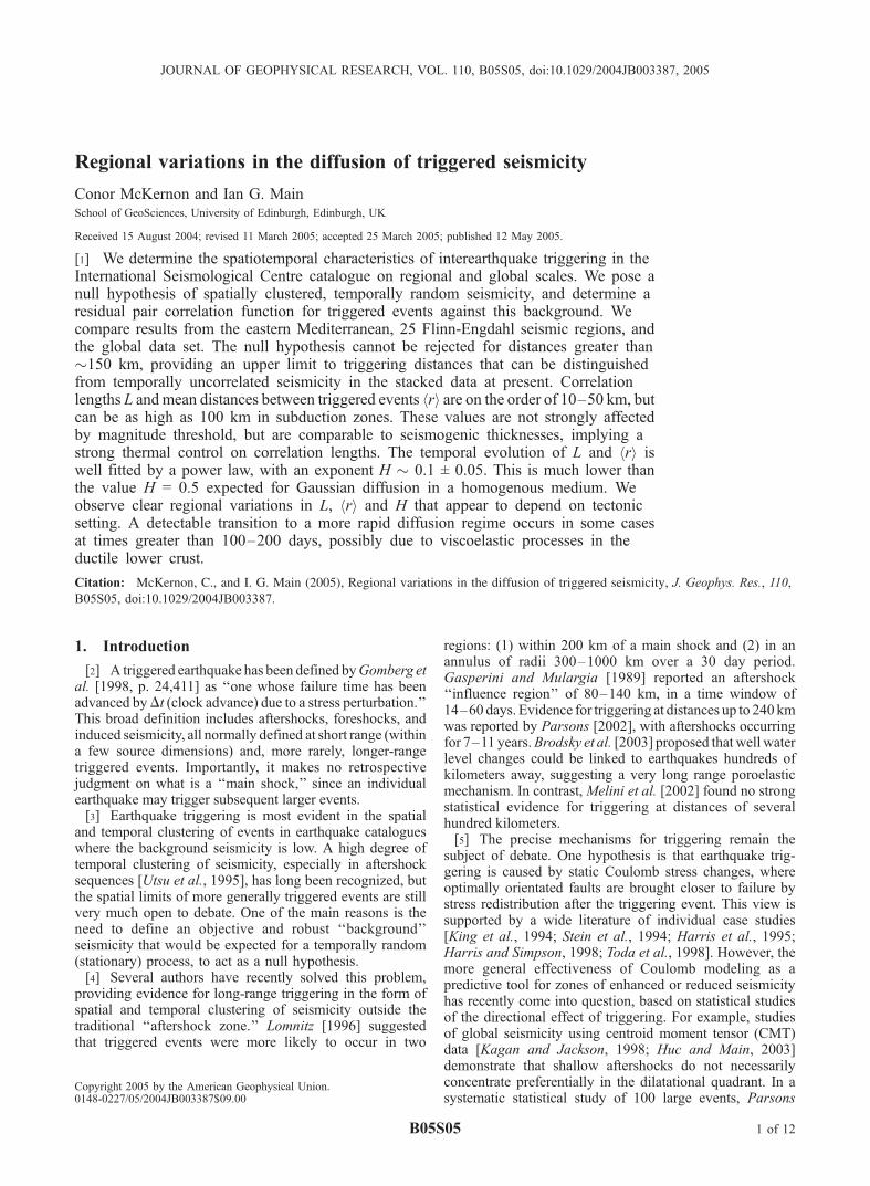
2 � NT)/2, assuming no prior knowledge ofthe spatial or temporal limits of any triggering effects. Wecalculate the time and distance separations for each trigger-triggered event pair, and then stack the data relative to theorigin time of the trigger event. The result is a series ofhistograms of distance versus number of pairs, using 5 kmbins, for a series of timewindows ranging from 1 to 1000 daysafter the triggering event. The raw histograms are corrected toaccount for the increasing surface area in successive annuli,using a standard Euclidean normalization [Lomnitz, 1995].An example is shown in Figure 1. All the histograms in thisstudy used 5 km increments, finer than the previous globalwork due to the smaller length scales involved at lower-magnitude threshold.[16] We then generate temporally random dates (random

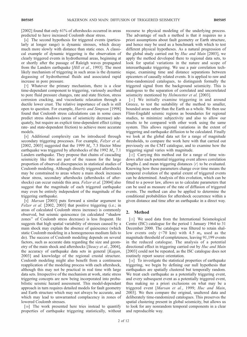
years, months and days separately) for the epicenterscontained in the ISC catalogue, and sort the new catalogueschronologically. We create 20 such time-randomized cata-logues, preserving the spatial distribution of seismicity, butremoving any underlying temporal connections that couldbe attributed to interearthquake triggering. Histograms arethen created for each of these 20 time-randomized cata-logues in the same manner as the original data, and anaverage histogram is obtained for the null hypothesis of aPoisson process. Figure 2 shows these histograms after thearea correction has been applied. We can now remove thebackground signal (as generated by the time-randomizedcatalogues) from the ‘‘real’’ signal, by subtracting theaveraged histogram from the real data histogram. The actual

physical triggering effect can then be interpreted to be theresidual pair correlation function left after this subtraction.This method can be applied for a range of time windows toevaluate the time dependence.[17] The pair correlation function for the triggered events

may be power law, an exponential, or a combination ofboth. Here we fit the data to the expression

N r; tð Þ ¼ Ar�ae�r=L; ð1Þ

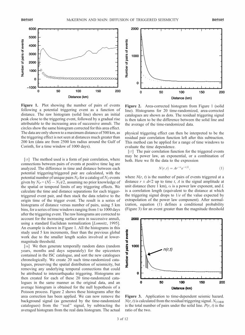
where N(r, t) is the number of pairs of events triggered at adistance r ± dr/2 up to time t, A is the signal amplitude atunit distance (here 1 km), a is a power law exponent, and Lis a correlation length (equivalent to the distance at whichthe triggering signal drops to 1/e of the value expected byextrapolation of the power law component). After normal-ization, equation (1) defines a conditional probability(Figure 3) for an event greater than the magnitude threshold

Figure 1. Plot showing the number of pairs of eventsfollowing a potential triggering event as a function ofdistance. The raw histogram (solid line) shows an initialpeak close to the triggering event, followed by a gradual riseattributable to the increasing area of successive annuli. Thecircles show the same histogram corrected for this area effect.The data are only shown to amaximum distance of 500 km, asthe triggering effect is not seen at distances much greater than200 km (data are from 2500 km radius around the Gulf ofCorinth, for a time window of 1000 days).

Figure 2. Area-corrected histogram from Figure 1 (solidline). Histograms for 20 time-randomized, area-correctedcatalogues are shown as dots. The residual triggering signalis then taken to be the difference between the solid line andthe average of the time-randomized data.

Figure 3. Application to time-dependent seismic hazard.N(r, t) is calculated from the residual triggering signal.NCORR

is the total number of pairs under the solid line. P(r, t) is theratio of the two.


3 of 12

B05S05

being triggered within a given annulus up to a time t: P(r, t) =N(r, t)/NCORR (where NCORR is the total number of pairs ofevents after the Euclidean area correction has been applied).This is useful in itself since it can be used directly forcalculating time-independent hazard (for the average popula-tion), conditional on the occurrence of previous events abovethe magnitude threshold. The relative influence of the powerlaw (short-range, r� L) and exponential (long-range, r� L)components of the distribution types can be determined fromthe data. Very long range triggering can then be definedfor r L.[18] We also determine the mean triggering distance:

hri tð Þ ¼X

r

rN r; tð ÞN r; tð Þ ; ð2Þ

where N(r, t) here is taken directly from the data, rather thana curve fit. Mean triggering distances are useful in that theyare independent of any statistical model or regressiontechnique. We then examine how L and hri evolve with timeby fitting them to power laws of the form:

L tð Þ ¼ L0 t=t0ð ÞH hri tð Þ ¼ hri0 t=t0ð ÞH ; ð3Þ

where L0 and hri0 are the correlation length and meantriggering distance, respectively for a minimum time t = t0,which must be greater than or equal to the minimum time atwhich the catalogue can be regarded as complete. L0 andhri0 represent the ‘‘direct effect,’’ or instantaneous responseto the stress perturbation. The power law exponent Hprovides a quantitative measure of the rate of (directly andindirectly) triggered earthquake diffusion. The diffusion of

triggered seismicity is in part controlled by the averageproperties of the percolation of stress outward from atriggering event, and as such H can also be thought of as anindicator of a (possibly stress related) diffusive process.

3. Results

3.1. Eastern Mediterranean

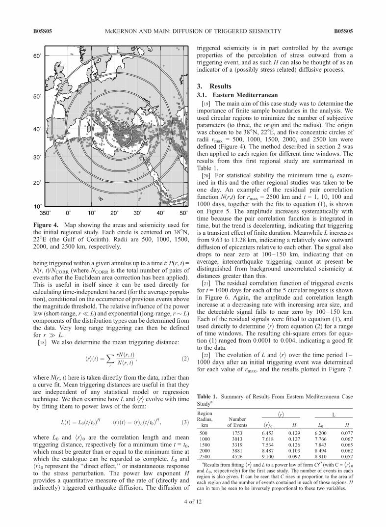
[19] The main aim of this case study was to determine theimportance of finite sample boundaries in the analysis. Weused circular regions to minimize the number of subjectiveparameters (to three, the origin and the radius). The originwas chosen to be 38�N, 22�E, and five concentric circles ofradii rmax = 500, 1000, 1500, 2000, and 2500 km weredefined (Figure 4). The method described in section 2 wasthen applied to each region for different time windows. Theresults from this first regional study are summarized inTable 1.[20] For statistical stability the minimum time t0 exam-

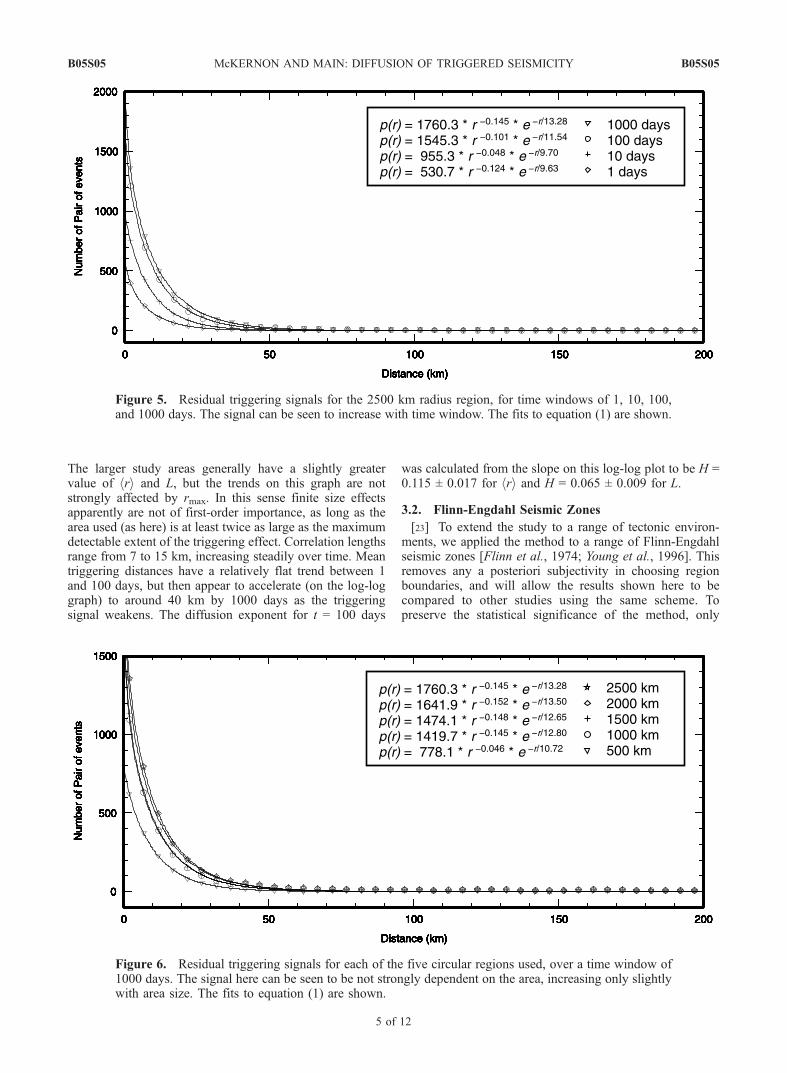
ined in this and the other regional studies was taken to beone day. An example of the residual pair correlationfunction N(r,t) for rmax = 2500 km and t = 1, 10, 100 and1000 days, together with the fits to equation (1), is shownon Figure 5. The amplitude increases systematically withtime because the pair correlation function is integrated intime, but the trend is decelerating, indicating that triggeringis a transient effect of finite duration. Meanwhile L increasesfrom 9.63 to 13.28 km, indicating a relatively slow outwarddiffusion of epicenters relative to each other. The signal alsodrops to near zero at 100–150 km, indicating that onaverage, interearthquake triggering cannot at present bedistinguished from background uncorrelated seismicity atdistances greater than this.[21] The residual correlation function of triggered events

for t = 1000 days for each of the 5 circular regions is shownin Figure 6. Again, the amplitude and correlation lengthincrease at a decreasing rate with increasing area size, andthe detectable signal falls to near zero by 100–150 km.Each of the residual signals were fitted to equation (1), andused directly to determine hri from equation (2) for a rangeof time windows. The resulting chi-square errors for equa-tion (1) ranged from 0.0001 to 0.004, indicating a good fitto the data.[22] The evolution of L and hri over the time period 1–

1000 days after an initial triggering event was determinedfor each value of rmax, and the results plotted in Figure 7.

Figure 4. Map showing the areas and seismicity used forthe initial regional study. Each circle is centered on 38�N,22�E (the Gulf of Corinth). Radii are 500, 1000, 1500,2000, and 2500 km, respectively.

Table 1. Summary of Results From Eastern Mediterranean Case

Studya

RegionRadius,km

Numberof Events

hri L

hri0 H L0 H

500 1753 6.453 0.129 6.200 0.0771000 3013 7.618 0.127 7.766 0.0671500 3319 7.534 0.126 7.843 0.0652000 3881 8.487 0.103 8.494 0.0622500 4526 9.100 0.092 8.910 0.052aResults from fitting hri and L to a power law of form CtH (with C = hri0

and L0, respectively) for the first case study. The number of events in eachregion is also given. It can be seen that C rises in proportion to the area ofeach region and the number of events contained in each of those regions. Hcan in turn be seen to be inversely proportional to these two variables.


4 of 12

B05S05

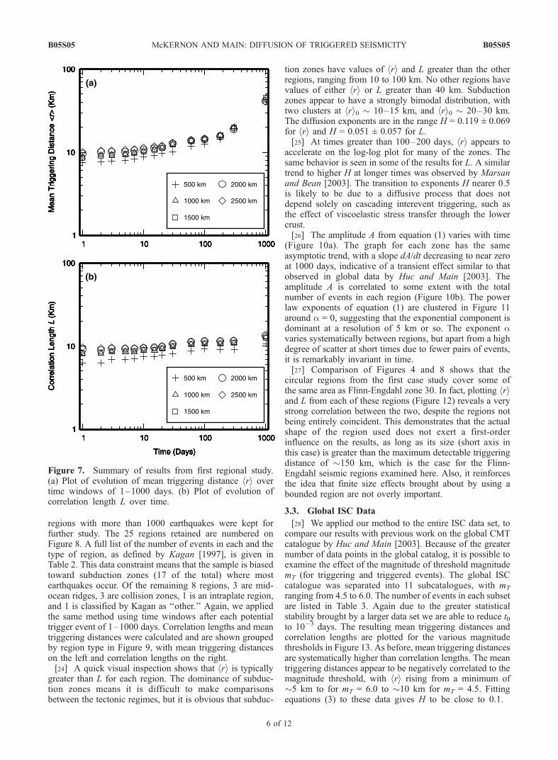
The larger study areas generally have a slightly greatervalue of hri and L, but the trends on this graph are notstrongly affected by rmax. In this sense finite size effectsapparently are not of first-order importance, as long as thearea used (as here) is at least twice as large as the maximumdetectable extent of the triggering effect. Correlation lengthsrange from 7 to 15 km, increasing steadily over time. Meantriggering distances have a relatively flat trend between 1and 100 days, but then appear to accelerate (on the log-loggraph) to around 40 km by 1000 days as the triggeringsignal weakens. The diffusion exponent for t = 100 days

was calculated from the slope on this log-log plot to be H =0.115 ± 0.017 for hri and H = 0.065 ± 0.009 for L.

3.2. Flinn-Engdahl Seismic Zones

[23] To extend the study to a range of tectonic environ-ments, we applied the method to a range of Flinn-Engdahlseismic zones [Flinn et al., 1974; Young et al., 1996]. Thisremoves any a posteriori subjectivity in choosing regionboundaries, and will allow the results shown here to becompared to other studies using the same scheme. Topreserve the statistical significance of the method, only

Figure 5. Residual triggering signals for the 2500 km radius region, for time windows of 1, 10, 100,and 1000 days. The signal can be seen to increase with time window. The fits to equation (1) are shown.

Figure 6. Residual triggering signals for each of the five circular regions used, over a time window of1000 days. The signal here can be seen to be not strongly dependent on the area, increasing only slightlywith area size. The fits to equation (1) are shown.


5 of 12

B05S05

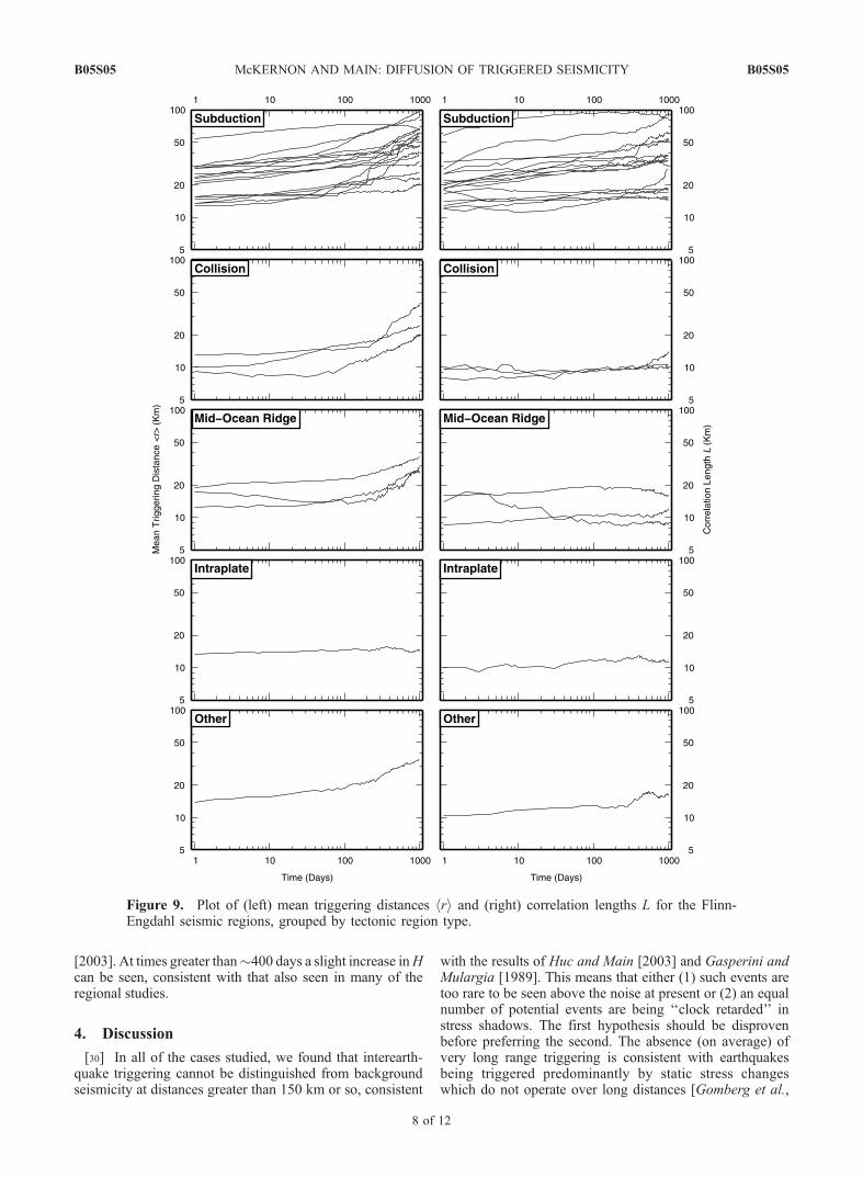
regions with more than 1000 earthquakes were kept forfurther study. The 25 regions retained are numbered onFigure 8. A full list of the number of events in each and thetype of region, as defined by Kagan [1997], is given inTable 2. This data constraint means that the sample is biasedtoward subduction zones (17 of the total) where mostearthquakes occur. Of the remaining 8 regions, 3 are mid-ocean ridges, 3 are collision zones, 1 is an intraplate region,and 1 is classified by Kagan as ‘‘other.’’ Again, we appliedthe same method using time windows after each potentialtrigger event of 1–1000 days. Correlation lengths and meantriggering distances were calculated and are shown groupedby region type in Figure 9, with mean triggering distanceson the left and correlation lengths on the right.[24] A quick visual inspection shows that hri is typically

greater than L for each region. The dominance of subduc-tion zones means it is difficult to make comparisonsbetween the tectonic regimes, but it is obvious that subduc-

tion zones have values of hri and L greater than the otherregions, ranging from 10 to 100 km. No other regions havevalues of either hri or L greater than 40 km. Subductionzones appear to have a strongly bimodal distribution, withtwo clusters at hri0 � 10–15 km, and hri0 � 20–30 km.The diffusion exponents are in the range H = 0.119 ± 0.069for hri and H = 0.051 ± 0.057 for L.[25] At times greater than 100–200 days, hri appears to

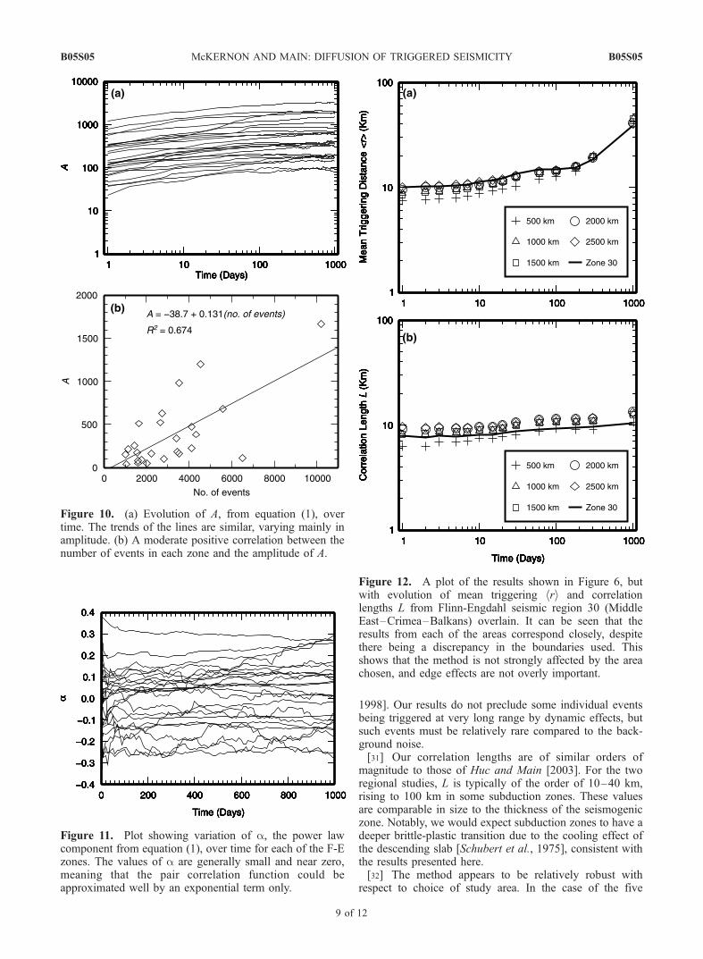
accelerate on the log-log plot for many of the zones. Thesame behavior is seen in some of the results for L. A similartrend to higher H at longer times was observed by Marsanand Bean [2003]. The transition to exponents H nearer 0.5is likely to be due to a diffusive process that does notdepend solely on cascading interevent triggering, such asthe effect of viscoelastic stress transfer through the lowercrust.[26] The amplitude A from equation (1) varies with time

(Figure 10a). The graph for each zone has the sameasymptotic trend, with a slope dA/dt decreasing to near zeroat 1000 days, indicative of a transient effect similar to thatobserved in global data by Huc and Main [2003]. Theamplitude A is correlated to some extent with the totalnumber of events in each region (Figure 10b). The powerlaw exponents of equation (1) are clustered in Figure 11around a = 0, suggesting that the exponential component isdominant at a resolution of 5 km or so. The exponent avaries systematically between regions, but apart from a highdegree of scatter at short times due to fewer pairs of events,it is remarkably invariant in time.[27] Comparison of Figures 4 and 8 shows that the

circular regions from the first case study cover some ofthe same area as Flinn-Engdahl zone 30. In fact, plotting hriand L from each of these regions (Figure 12) reveals a verystrong correlation between the two, despite the regions notbeing entirely coincident. This demonstrates that the actualshape of the region used does not exert a first-orderinfluence on the results, as long as its size (short axis inthis case) is greater than the maximum detectable triggeringdistance of �150 km, which is the case for the Flinn-Engdahl seismic regions examined here. Also, it reinforcesthe idea that finite size effects brought about by using abounded region are not overly important.

3.3. Global ISC Data

[28] We applied our method to the entire ISC data set, tocompare our results with previous work on the global CMTcatalogue by Huc and Main [2003]. Because of the greaternumber of data points in the global catalog, it is possible toexamine the effect of the magnitude of threshold magnitudemT (for triggering and triggered events). The global ISCcatalogue was separated into 11 subcatalogues, with mT

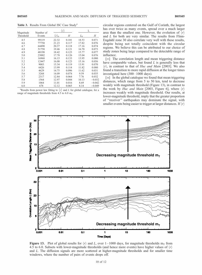
ranging from 4.5 to 6.0. The number of events in each subsetare listed in Table 3. Again due to the greater statisticalstability brought by a larger data set we are able to reduce t0to 10�3 days. The resulting mean triggering distances andcorrelation lengths are plotted for the various magnitudethresholds in Figure 13. As before, mean triggering distancesare systematically higher than correlation lengths. The meantriggering distances appear to be negatively correlated to themagnitude threshold, with hri rising from a minimum of�5 km to for mT = 6.0 to �10 km for mT = 4.5. Fittingequations (3) to these data gives H to be close to 0.1.

Figure 7. Summary of results from first regional study.(a) Plot of evolution of mean triggering distance hri overtime windows of 1–1000 days. (b) Plot of evolution ofcorrelation length L over time.


6 of 12

B05S05

[29] The diffusion exponent H for each threshold variesfor hri from �0.049 for mT = 6.0 data to 0.133 for mT = 5.1.Similar results can be seen for the correlation lengths, butbreak down somewhat at the higher-magnitude thresholdsand shorter time separations due to a lack of events in thecatalogues. For example, the data set for mT = 6.0 contains

only 678 earthquakes spread over the entire globe. Fittingsuch noisy data to equation (1) appears to be unstable abovemagnitude thresholds of 5.0 mb. Below 5.0 mb, the resultsshow trends similar to those seen in the regional studies of hri,but again of lower amplitude.Mean triggering distances rangefrom 10 to 25 km, similar to those observed byHuc andMain

Figure 8. Map of Flinn-Engdahl seismic regions, with regions used in study outlined and numbered.

Table 2. Summary of Results From Flinn-Engdahl Case Studya

F-E Region Name Number of Events Region Type

hri L

hri0 H L0 H

1 Alaska-Aleutian Arc 5585 subduction 57.716 0.037 70.308 0.0505 Mexico-Guatemala 2013 subduction 20.438 0.129 20.482 0.0886 Central America 1775 subduction 26.346 0.112 27.192 0.0897 Caribbean Loop 1133 subduction 14.817 0.034 15.419 0.0118 Andean South America 4119 subduction 23.457 0.057 20.542 0.06912 Kermadec-Tonga-Samoa Basin 6489 subduction 21.879 0.192 17.848 0.16914 Vanuatu Islands 4140 subduction 19.309 0.116 19.879 0.07415 Bismarck-Solomon Islands 4308 subduction 22.748 0.128 20.700 0.11916 New Guinea 3416 subduction 22.633 0.123 25.311 0.02818 Guam-Japan 2734 subduction 13.199 0.099 11.671 0.07319 Japan-Kamchatka 10187 subduction 28.460 0.062 33.991 0.01220 SE Japan-Ryukyu Islands 1420 subduction 9.275 0.189 17.610 0.00021 Taiwan 1664 subduction 14.465 0.066 14.179 0.00922 Philippines 4552 subduction 17.384 0.138 18.354 0.08423 Borneo-Sulawesi 3553 subduction 6.024 0.319 8.475 0.14124 Sunda Arc 3451 subduction 25.845 0.176 35.031 0.12446 Andaman Islands-Sumatera 1028 subduction 11.701 0.136 13.661 0.02026 India-Xizand-Sichuan-Yunnan 1555 collision 6.263 0.141 8.773 0.03329 Western Asia 2212 collision 11.094 0.097 9.393 0.00330 Middle East-Crimea-Balkans 2657 collision 6.101 0.237 7.419 0.04737 Africa 1039 intracontinental 13.506 0.013 9.582 0.03232 Atlantic Ocean 3519 mid-ocean ridge 9.448 0.132 8.523 0.04533 Indian Ocean 2832 mid-ocean ridge 17.304 0.085 16.325 0.02043 SE and Antarctic Pacific Ocean 1596 mid-ocean ridge 14.696 0.029 16.586 �0.11810 Southern Antilles 1619 other 11.641 0.135 10.155 0.055

aResults from fitting hri = hri0(t/t0)H for the mean triggering distances and L = L0(t/t0)H for the correlation lengths from the Flinn-Engdahl case study.

Regions are grouped by types put forward by Kagan [1997].


7 of 12

B05S05

[2003]. At times greater than�400 days a slight increase inHcan be seen, consistent with that also seen in many of theregional studies.

4. Discussion

[30] In all of the cases studied, we found that interearth-quake triggering cannot be distinguished from backgroundseismicity at distances greater than 150 km or so, consistent

with the results of Huc and Main [2003] and Gasperini andMulargia [1989]. This means that either (1) such events aretoo rare to be seen above the noise at present or (2) an equalnumber of potential events are being ‘‘clock retarded’’ instress shadows. The first hypothesis should be disprovenbefore preferring the second. The absence (on average) ofvery long range triggering is consistent with earthquakesbeing triggered predominantly by static stress changeswhich do not operate over long distances [Gomberg et al.,

Figure 9. Plot of (left) mean triggering distances hri and (right) correlation lengths L for the Flinn-Engdahl seismic regions, grouped by tectonic region type.


8 of 12

B05S05

1998]. Our results do not preclude some individual eventsbeing triggered at very long range by dynamic effects, butsuch events must be relatively rare compared to the back-ground noise.[31] Our correlation lengths are of similar orders of

magnitude to those of Huc and Main [2003]. For the tworegional studies, L is typically of the order of 10–40 km,rising to 100 km in some subduction zones. These valuesare comparable in size to the thickness of the seismogeniczone. Notably, we would expect subduction zones to have adeeper brittle-plastic transition due to the cooling effect ofthe descending slab [Schubert et al., 1975], consistent withthe results presented here.[32] The method appears to be relatively robust with

respect to choice of study area. In the case of the five

Figure 10. (a) Evolution of A, from equation (1), overtime. The trends of the lines are similar, varying mainly inamplitude. (b) A moderate positive correlation between thenumber of events in each zone and the amplitude of A.

Figure 11. Plot showing variation of a, the power lawcomponent from equation (1), over time for each of the F-Ezones. The values of a are generally small and near zero,meaning that the pair correlation function could beapproximated well by an exponential term only.

Figure 12. A plot of the results shown in Figure 6, butwith evolution of mean triggering hri and correlationlengths L from Flinn-Engdahl seismic region 30 (MiddleEast–Crimea–Balkans) overlain. It can be seen that theresults from each of the areas correspond closely, despitethere being a discrepancy in the boundaries used. Thisshows that the method is not strongly affected by the areachosen, and edge effects are not overly important.


9 of 12

B05S05

circular regions centered on the Gulf of Corinth, the largesthas over twice as many events, spread over a much largerarea than the smallest one. However, the evolution of hriand L for both are very similar. The results from Flinn-Engdahl zone 30 also correlate very well with these results,despite being not totally coincident with the circularregions. We believe this can be attributed to our choice ofstudy zones being large compared to the detectable range ofinfluence.[33] The correlation length and mean triggering distance

have comparable values, but found L is generally less thathri, in contrast to that of Huc and Main [2003]. We alsofound a transition to more rapid diffusion at the longer timesinvestigated here (300–1000 days).[34] In the global catalogue we found that mean triggering

distances, which range from 5 to 50 km, tend to decreaseweakly with magnitude threshold (Figure 13), in contrast tothe work by Huc and Main [2003, Figure 6], where hriincreases weakly with magnitude threshold. Our results, atlower-magnitude threshold, imply that the greater proportionof ‘‘receiver’’ earthquakes may dominate the signal, withsmaller events being easier to trigger at larger distances. If hri

Table 3. Results From Global ISC Case Studya

MagnitudeThreshold

Number ofEvents

hri L

hri0 H L0 H

4.5 99119 22.32 0.101 18.53 0.0714.6 77750 21.23 0.117 17.82 0.0764.7 64490 20.37 0.118 17.16 0.0744.8 51758 19.46 0.121 16.70 0.0734.9 40198 18.42 0.123 15.77 0.0775.0 23002 17.78 0.126 15.04 0.0765.1 16968 16.15 0.133 13.95 0.0805.2 12447 16.08 0.123 15.16 0.0565.3 9003 15.34 0.119 13.91 0.0705.4 6426 13.99 0.114 11.82 0.0805.5 4629 14.75 0.096 11.62 0.0315.6 3268 14.09 0.074 9.59 0.0355.7 2317 12.84 0.064 7.76 0.0325.8 1564 12.97 0.044 10.13 �0.0325.9 1064 11.01 0.016 8.69 �0.0426.0 678 12.12 0.065 8.14 �0.049

aResults from power law fitting to hri and L for global catalogue, for arange of magnitude thresholds from 4.5 to 6.0 mb.

Figure 13. Plot of global results for hri and L, over 1–1000 days, for magnitude thresholds mT from4.5 to 6.0. Subsets with lower-magnitude thresholds (and hence more events) have higher values of hriand L. The diffusion signals are more scattered at higher-magnitude thresholds and for smaller timewindows, where the number of pairs of events drops off.


10 of 12

B05S05

is relatively insensitive, or even independent of magnitudethreshold (e.g., as in the work by Felzer et al. [2004]) thencorrelation lengthmust be determined a priori by factors otherthan the triggering magnitude threshold, most likely theseismogenic thickness. The correlation length may alsoappear to decrease with time if the magnitude threshold istoo high (Figure 13), most likely due to statistical instabilityassociated with having fewer pairs of events. Similarly atshorter times there is greater scatter in the data, also due to thelack of potential triggering-triggered pairs. The results ofFigure 13 also show similar effects for hri but to a lesserdegree, implying that hri is more robust than model-dependent parameters such as L.[35] The mean triggering distance at a given time is

relatively insensitive to the magnitude threshold, at leastup to magnitude 6 or so (Figure 13). Such an event wouldhave a source dimension comparable to the seismogenicthickness. For trigger magnitude thresholds much greaterthan this we may expect correlation lengths along strike toexceed those found here, due to the fact that the sourcedimension is greater than the seismogenic thickness. Withcurrent data it is not possible to test this hypothesis. Again itis important to emphasis that we have plotted the statisticalaverage of the population as a function of the completenessthreshold, and not the response of the earth to a triggeringevent of a specific magnitude.[36] For the easternMediterranean studyH = 0.115 ± 0.017

for hri andH = 0.065 ± 0.009 for hri L, withmT = 4.5. For theFlinn-Engdahl regions, we find H = 0.119 ± 0.069 and H =0.051 ± 0.057 for mT = 4.5. In the case of the global catalogs,H = 0.049 ± 0.047 and H =�0.026 ± 0.090, again calculatedfrom hri and L, respectively. The low values of H areconsistent with the work byMarsan et al. [2000], who foundH to be 0.1 for mining-induced seismicity, and 0.22 at theLong Valley caldera and in southern California. Marsan andBean [2003] calculatedH at a global scale (for the Council ofthe National Seismic System catalogue, 1963–1998,M 5,depth � 70 km) to be bimodal. For times spanning 10�3 to10 days,H = 0.19, and for times over the range 10 to 103 days,Hwas shown to be 0.4, significantly higher than any values ofH derived here. They found H to be 0.37 for ocean ridges,higher by more than 0.2 compared to those listed in Table 2.They also report a positive correlation between heat flow andH, suggesting a strong thermal control (consistent in turnwithseismogenic depth being a strong determinant of correlationlength, since low heat flow leads to a deeper brittle/ductiletransition). Comparing physical parameters such as heat flow,crustal thickness, or relative plate velocities would be anatural progression of the regional analysis presented herebut with current data would require either narrowing the sizeof the zones to the correlation length of heat flow data(thereby reducing the statistical stability) or a major coarsegraining of data to match the size of the F-E zones (reducingthe resolution).[37] Helmstetter et al. [2003] calculated values of H for

21 main shock sequences in California, using two methodsto remove the background, or uncorrelated, seismicity. Forthe first method, using a windowing technique, they foundH ranging between 0.01 and 0.41, with a mean of 0.08 ±0.09, similar to the range reported here. Their secondtechnique (using a wavelet method to remove the uncorre-lated seismicity) produced values of H ranging between

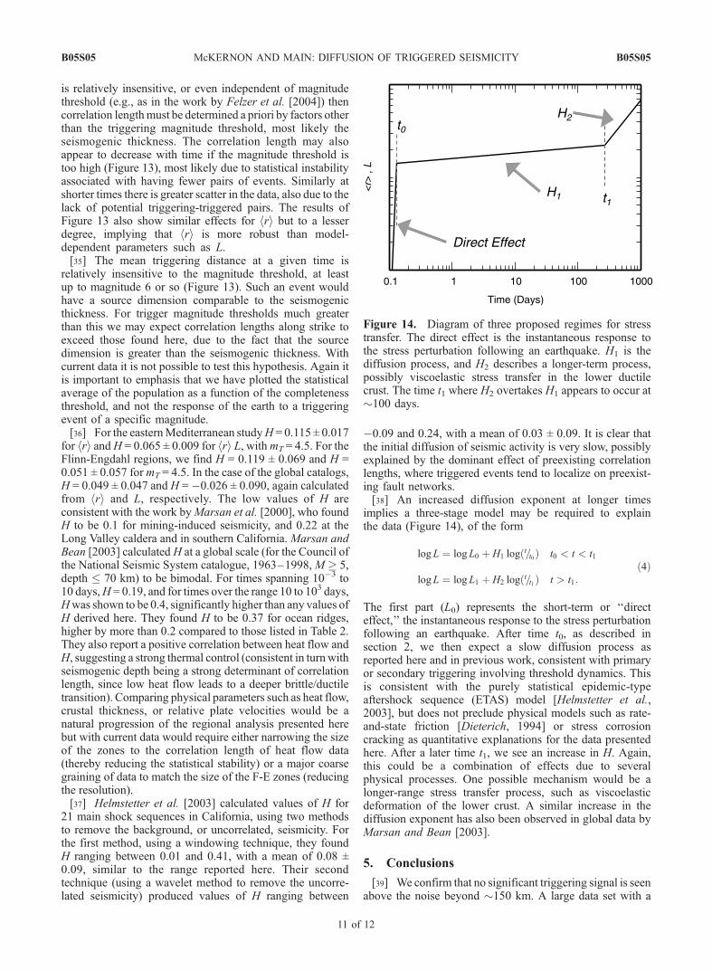
�0.09 and 0.24, with a mean of 0.03 ± 0.09. It is clear thatthe initial diffusion of seismic activity is very slow, possiblyexplained by the dominant effect of preexisting correlationlengths, where triggered events tend to localize on preexist-ing fault networks.[38] An increased diffusion exponent at longer times

implies a three-stage model may be required to explainthe data (Figure 14), of the form

logL ¼ logL0 þ H1 logt=t0ð Þ t0 < t < t1

logL ¼ logL1 þ H2 logt=t1ð Þ t > t1:

ð4Þ

The first part (L0) represents the short-term or ‘‘directeffect,’’ the instantaneous response to the stress perturbationfollowing an earthquake. After time t0, as described insection 2, we then expect a slow diffusion process asreported here and in previous work, consistent with primaryor secondary triggering involving threshold dynamics. Thisis consistent with the purely statistical epidemic-typeaftershock sequence (ETAS) model [Helmstetter et al.,2003], but does not preclude physical models such as rate-and-state friction [Dieterich, 1994] or stress corrosioncracking as quantitative explanations for the data presentedhere. After a later time t1, we see an increase in H. Again,this could be a combination of effects due to severalphysical processes. One possible mechanism would be alonger-range stress transfer process, such as viscoelasticdeformation of the lower crust. A similar increase in thediffusion exponent has also been observed in global data byMarsan and Bean [2003].

5. Conclusions

[39] We confirm that no significant triggering signal is seenabove the noise beyond �150 km. A large data set with a

Figure 14. Diagram of three proposed regimes for stresstransfer. The direct effect is the instantaneous response tothe stress perturbation following an earthquake. H1 is thediffusion process, and H2 describes a longer-term process,possibly viscoelastic stress transfer in the lower ductilecrust. The time t1 where H2 overtakes H1 appears to occur at�100 days.


11 of 12

B05S05

lower threshold of completeness has allowed us to apply ourmethod to different tectonic regimes. The residual triggeringsignals, towhich equation (1) is fitted, determine a probabilitydistribution of triggered events conditional on the occurrenceof a triggering event. As such they could be used afterappropriate normalization as estimates of conditional proba-bilities for time-dependant seismic hazard as an average forthe population as a whole. Correlation lengths L and meantriggering distances hri are found to be on the order of10–40 km in most cases, with the exception of subductionzones, where they range over 10–100 km. This may be due tovariations in seismogenic thickness; for example, rapidlydescending subduction zones will have a deeper brittle-ductile transition due to thermal cooling. Subduction zonesdisplay a bimodal distribution in L and hri.[40] Our values of hri and L are higher than those derived

at higher-magnitude threshold from the CMT catalog.Exponents determined from hri are generally larger thanwhen calculated from L. For the eastern Mediterranean H =0.115 ± 0.017 for hri and H = 0.065 ± 0.009 for L. For theFlinn-Engdahl case study H = 0.119 ± 0.069 for hri and H =0.051 ± 0.057 for hLi. For the global catalogs, H = 0.049 ±0.047 for hri and H = �0.026 ± 0.090 for L. All are muchlower than 0.5, the value for a homogenous Fickian diffu-sion process, implying strong preexisting crustal heteroge-neity. The values of H for the global study tend to be smallerthan those calculated by Huc and Main [2003] from theCMT catalog (0.05 < H < 0.06). The global values of hriand L show a systematic increase with decreasing magni-tude threshold, implying smaller events may be easier totrigger.

[41] Acknowledgments. This work was funded by NERC Student-ship NER/S/A/2001/06166 and also in part by the Corinth Rift Laboratory(http://www.Corinth-rift-lab.org), a European Union funded project. Wethank Associate Editor Massimo Cocco, Frank Evans and two anonymousreviewers for their constructive and detailed reviews, and Bruce Malamudfor comments during the course of the work.

ReferencesBrodsky, E. E., E. Roeloffs, D. Woodcock, I. Gall, and M. Manga (2003), Amechanism for sustained groundwater pressure changes induced by dis-tant earthquakes, J. Geophys. Res., 108(B8), 2390, doi:10.1029/2002JB002321.

Dieterich, J. (1994), A constitutive law for rate of earthquake productionand its application to earthquake clustering, J. Geophys. Res., 99(B2),2601–2618.

Felzer, K. R., T. W. Becker, R. E. Abercrombie, G. Ekstrom, and J. R. Rice(2002), Triggering of the 1999 MW 7.1 Hector Mine earthquake by after-shocks of the 1992 MW 7.3 Landers earthquake, J. Geophys. Res.,107(B9), 2190, doi:10.1029/2001JB000911.

Felzer, K. R., R. E. Abercrombie, and G. Ekstrom (2003), Secondary after-shocks and their importance for aftershock forecasting, Bull. Sesimol.Soc. Am., 93, 1433–1448.

Felzer, K. R., R. E. Abercrombie, and G. Ekstrom (2004), A common originfor aftershocks, foreshocks, and multiplets, Bull. Sesimol. Soc. Am., 94,88–98.

Flinn, E. A., E. R. Engdahl, and A. R. Hill (1974), Seismic and geographi-cal regionalization, Bull. Seismol. Soc. Am., 64, 771–993.

Gasperini, P., and F. Mulargia (1989), A statistical analysis of seismicity inItaly: The clustering properties, Bull. Seismol. Soc. Am., 79, 973–988.

Gomberg, J., N. M. Beeler, M. L. Blanpied, and P. Bodin (1998), Earth-quake triggering by transient and static deformations, J. Geophys. Res.,103(B10), 24,411–24,426.

Harris, R. A., and R. W. Simpson (1998), Suppression of large earthquakesby stress shadows: A comparison of Coulomb and rate-and-state failure,J. Geophys. Res., 103(B10), 24,439–24,451.

Harris, R. A., R. W. Simpson, and P. A. Reasenberg (1995), Influence ofstatic stress changes on earthquake locations in southernCalifornia,Nature,375, 221–224.

Helmstetter, A., G. Ouillon, and D. Sornette (2003), Are aftershocks oflarge Californian earthquakes diffusing?, J. Geophys. Res., 108(B10),2483, doi:10.1029/2003JB002503.

Hill, D. P., et al. (1993), Seismicity remotely triggered by the magnitude 7.1Landers, California, earthquake, Science, 260, 1617–1623.

Huc, M., and I. G. Main (2003), Anomalous stress diffusion in earthquaketriggering: Correlation length, time dependence, and directionality, J. Geo-phys. Res., 108(B7), 2324, doi:10.1029/2001JB001645.

Kagan, Y. Y. (1997), Seismic moment-frequency relation for shallowearthquakes: Regional comparison, J. Geophys. Res., 102(B2),2835–2852.

Kagan, Y. Y. (2003), Accuracy of modern global earthquake catalogs, Phys.Earth Planet. Inter., 135, 173–209.

Kagan, Y. Y., and D. D. Jackson (1998), Spatial aftershock distribution:Effect of normal stress, J. Geophys. Res., 103(B10), 24,453–24,467.

King, G. C. P., R. S. Stein, and J. Lin (1994), Static stress changes and thetriggering of earthquakes, Bull. Seismol. Soc. Am., 84, 935–953.

Lomnitz, C. (1995), On the distribution of distances between random pointson a sphere, Bull. Seismol. Soc. Am., 85, 951–953.

Lomnitz, C. (1996), Search of a worldwide catalog for earthquakes trig-gered at intermediate distances, Bull. Seismol. Soc. Am., 86, 293–298.

Marsan, D. (2003), Triggering of seismicity at short timescales followingCalifornian earthquakes, J. Geophys. Res., 108(B5), 2266, doi:10.1029/2002JB001946.

Marsan, D., and C. J. Bean (2003), Seismicity response to stress perturba-tions, analysed for a world-wide catalogue, Geophys. J. Int., 154, 179–195.

Marsan, D., C. J. Bean, S. Steacy, and J. McCloskey (1999), Spatio-temporalanalysis of stress diffusion in mining induced seismicity, Geophys. Res.Lett., 26, 3697–3700.

Marsan, D., C. J. Bean, S. Steacy, and J. McClosky (2000), Observation ofdiffusion processes in earthquake populations and implications for theirpredictability of seismicity systems, J. Geophys. Res., 105(B12),28,081–28,094.

Melini, D., A. Casarotti, A. Piersanti, and E. Boschi (2002), New insightson long range fault interactions, Earth Planet. Sci. Lett., 204, 363–372.

Parsons, T. (2002), Global Omori law decay of triggered earthquakes: Largeaftershocks outside the classical aftershock zone, J. Geophys. Res.,107(B9), 2199, doi:10.1029/2001JB000646.

Schubert, G., D. A. Yuenm, and D. L. Turcotte (1975), Role of phasetransitions in a dynamic mantle, Geophys. J. R. Astron. Soc., 42(2),705–735.

Steacy, S., D. Marsan, S. S. Nalbant, and J. McCloskey (2004), Sensitivityof static stress calculations to the earthquake slip distribution, J. Geophys.Res., 109, B04303, doi:10.1029/2002JB002365.

Stein, R. S., G. C. P. King, and J. Lin (1994), Stress triggering of the 1994M = 6.7 Northridge, California, earthquake by its predecessors, Science,265, 1432–1435.

Toda, S., R. S. Stein, P. A. Reasenberg, and J. H. Dieterich (1998), Stresstransferred by the Mw = 6.9 Kobe, Japan, shock: Effect on aftershocksand future earthquake probabilities, J. Geophys. Res., 103(B10), 24,543–24,565.

Utsu, T., Y. Ogata, and S. Matsu’ura (1995), The centenary of the Omoriformula for a decay law of aftershock activity, J. Phys. Earth., 43, 1–33.

Young, J. B., B. W. Presgrave, H. Aichele, D. A. Wiens, and E. A. Flinn(1996), The Flinn-Engdahl regionalization scheme: The 1995 revision,Phys. Earth Planet. Inter., 96, 223–297.

��I. G. Main and C. McKernon, School of GeoSciences, University of

Edinburgh, West Mains Road, Edinburgh, Midlothian EH9 3JW, UK.([email protected]; [email protected])


12 of 12

B05S05

regional variations in the diffusion of triggered … variations in the diffusion of triggered...

Documents