regionalizing nonparametric models of precipitation

Hydrol. Earth Syst. Sci., 21, 2463–2481, 2017www.hydrol-earth-syst-sci.net/21/2463/2017/doi:10.5194/hess-21-2463-2017© Author(s) 2017. CC Attribution 3.0 License.

Regionalizing nonparametric models of precipitation amounts ondifferent temporal scalesTobias Mosthaf and András BárdossyInstitute for Modeling Hydraulic and Environmental Systems, Universität Stuttgart, Stuttgart, Germany

Correspondence to: Tobias Mosthaf ([email protected])

Received: 2 September 2016 – Discussion started: 17 October 2016Revised: 29 March 2017 – Accepted: 9 April 2017 – Published: 10 May 2017

Abstract. Parametric distribution functions are commonlyused to model precipitation amounts corresponding to dif-ferent durations. The precipitation amounts themselves arecrucial for stochastic rainfall generators and weather gener-ators. Nonparametric kernel density estimates (KDEs) offera more flexible way to model precipitation amounts. As al-ready stated in their name, these models do not exhibit pa-rameters that can be easily regionalized to run rainfall gen-erators at ungauged locations as well as at gauged locations.To overcome this deficiency, we present a new interpolationscheme for nonparametric models and evaluate it for dif-ferent temporal resolutions ranging from hourly to monthly.During the evaluation, the nonparametric methods are com-pared to commonly used parametric models like the two-parameter gamma and the mixed-exponential distribution. Aswater volume is considered to be an essential parameter forapplications like flood modeling, a Lorenz-curve-based crite-rion is also introduced. To add value to the estimation of dataat sub-daily resolutions, we incorporated the plentiful dailymeasurements in the interpolation scheme, and this idea wasevaluated. The study region is the federal state of Baden-Württemberg in the southwest of Germany with more than500 rain gauges. The validation results show that the newlyproposed nonparametric interpolation scheme provides rea-sonable results and that the incorporation of daily values inthe regionalization of sub-daily models is very beneficial.

1 Introduction

Rainfall time series of differing temporal resolutions areneeded for various applications like water engineering de-sign, flood modeling, risk assessments and ecosystem and

hydrological impact studies (Wilks and Wilby, 1999; Bur-ton et al., 2008). As many precipitation records are too shortand contain erroneous measurements, stochastic precipita-tion models can be used to generate synthetic time seriesinstead. Starting from single-site models (summarized inWilks and Wilby, 1999) and multisite models for simulta-neous time series at various sites (e.g., Wilks, 1998; Buis-hand and Brandsma, 2001; Bárdossy and Plate, 1992), mod-els that allow for gridded simulations are finally developed(e.g., Wilks, 2009; Burton et al., 2008).

For modeling precipitation, one crucial variable is the pre-cipitation amount, which follows a certain distribution. Dis-tributions of the daily precipitation amounts are stronglyright skewed, with many small values and few large values(Wilks and Wilby, 1999; Li et al., 2012; Chen and Brissette,2014). This also holds true for different temporal resolu-tions with increasing skewness for higher temporal resolu-tions and vice versa. This means that rainfall intensity distri-butions depend on the temporal scale of the observed values.Applying single-site or multisite precipitation models at un-gauged locations requires the regionalization of the precipi-tation amount distributions. This can be done in two differentways.

1. Interpolate the precipitation amounts from observationpoints for every time step to the target location(s) andset up a distribution with the interpolated values.

2. Fit a distribution function to the precipitation amountsseparately for each gauge and interpolate the distribu-tion functions to the target location(s).

The first approach seems more straightforward, but exhibitsseveral deficiencies, such as the overestimation of the rain-fall probability, the underestimation of the variance and the

Published by Copernicus Publications on behalf of the European Geosciences Union.

2464 T. Mosthaf and A. Bárdossy: Regionalizing nonparametric models of precipitation amounts

underestimation of the maximum rainfall value. In the Sup-plement Sect. S1, an example demonstrates these problems.Due to the relative inefficiency of the first interpolation ap-proach, the second is preferred.

In most stochastic rainfall models, the theoretical paramet-ric distribution functions are fitted to the empirical values us-ing, e.g., the exponential distribution or the two-parametricgamma distribution (Wilks and Wilby, 1999; Papalexiou andKoutsoyiannis, 2012). It is possible to either interpolate theparameters of the theoretical distribution or to interpolate themoments (e.g., the mean and standard deviation) of the rain-fall intensities (Wilks, 2008; Haberlandt, 1998). Lall et al.(1996) introduced a more flexible nonparametric single-siterainfall model, for which they used nonparametric KDEswith a prior logarithmic transformation to model daily rain-fall intensities. They addressed the problem of regionaliza-tion by using nonparametric estimates of distribution func-tions. However, a different interpolation scheme is requiredfor nonparametric estimations, as they do not use any param-eter that can be simply interpolated.

In the present work, we introduce a regionalization strat-egy for nonparametric distributions and compare it to the tra-ditional regionalization of parametric distributions for vary-ing temporal resolutions from hourly to monthly scales.The common procedure to interpolate parametric distributionfunctions is outlined as follows.

1. Fit a parametric distribution (e.g., a gamma or exponen-tial distribution) at each sampling site to the empiricaldistribution function (EDF).

2. Interpolate the moment(s) or parameter(s) of the fittedparametric distribution.

3. Set up the theoretical cumulative distribution function(CDF) at every interpolation target with the interpolatedmoment(s) or parameter(s).

The newly proposed procedure for the nonparametric dis-tribution functions is the following.

1. Fit a nonparametric distribution to log-transformed rain-fall values using a Gaussian kernel.

2. Estimate the interpolation (kriging) weights with theprecipitation values of a certain quantile.

3. Apply these weights to the values of certain discretequantiles.

4. Linearly interpolate the remaining quantile values to re-ceive a continuous CDF for all target locations.

In Arns et al. (2013), a similar approach is used to in-terpolate the quantile value differences of water levels fora bias correction between the empirical distributions of theobserved and modeled values at the German North Sea

coast. In contrast to their work, entire theoretical distribu-tion functions are estimated in our work through interpola-tion. Goulard and Voltz (1993) introduced a curve krigingprocedure to regionalize fitted functions, which was furtherdeveloped by Giraldo et al. (2011). Based on their work,Menafoglio et al. (2013) developed a universal kriging ap-proach for the nonstationary interpolation of functional data,which was applied in Menafoglio et al. (2016) for the simu-lation of soil particle distribution functions. As CDF curvesare special functions that are monotonically non-decreasingbetween 0 and 1, the curve kriging procedure additionallyneeds to be constrained to these conditions. Our approachcan deal with these conditions directly.

After describing the study region Baden-Württemberg inSect. 2, the concept of precipitation amount models is intro-duced in Sect. 3. The data selection in Sect. 4 is followedby an investigation of the spatial dependence of the precipi-tation amount models in Sect. 5. The theory of precipitationamount models is addressed in Sect. 6, and the basis of theproposed interpolation procedure for nonparametric modelsis established in Sect. 7. The application of different region-alization procedures for precipitation amount models is ex-plained in Sect. 8. The implementation of daily rainfall ob-servations within the interpolation of sub-daily distributionfunctions is outlined in Sect. 9. The resulting performance ofthe different precipitation amount models at the point loca-tions and their regionalization is depicted in Sect. 10.

2 Study region and data

The study region is the federal state of Baden-Württemberg,which is located in the southwest of Germany. The BlackForest mountain range, in the west, and the Swabian Alps,extending from southwest to northeast, exhibit the high-est elevations in Baden-Württemberg. The rising of large-scale moist air masses across the mountainous regions causeshigher rainfall amounts on the windward side and loweramounts on the leeward side. In the summer months, slopeswith differing inclinations lead to a warming of the air thattriggers convection currents, leading to a greater number ofshowers and thunderstorms over the mountainous regions.This shows a dependence of rainfall on elevation with sea-sonal differences. The rain-bearing westerly winds lead tohigh rainfall amounts in the Black Forest. The relativelylower altitude of the Swabian Alps results in lower rainfallamounts as they lie in the shadow of the Black Forest (Lan-desanstalt für Umwelt, Messungen und Naturschutz Baden-Württemberg , LUBW).

The years from 1997 to 2011 are chosen as the investiga-tion period, as the German Meteorological Service (DWD)set up many new rain gauges in 1997. A relatively homo-geneous data set is obtained by only choosing gauges withobservation periods greater than or equal to 5 years, whichalso provide rainfall measurements for at least 80 % of the

Hydrol. Earth Syst. Sci., 21, 2463–2481, 2017 www.hydrol-earth-syst-sci.net/21/2463/2017/

T. Mosthaf and A. Bárdossy: Regionalizing nonparametric models of precipitation amounts 2465

Figure 1. The locations of the high-resolution (hourly and 5 min; a) and daily rain gauges (b) in Baden-Württemberg.

time steps within their observation period. We had access to(i) 242 hourly and 5 min resolution and (ii) 347 daily gaugesavailable in the study region, with 80 sites having both dailyand high-resolution instruments. The observations are pro-vided by the DWD and the Environmental Agency of Baden-Württemberg (LUBW). The high-resolution rain gauges aremostly equipped with tipping buckets and gravimetric mea-surement devices (Beck, 2013). Figure 1 shows the study re-gion with the locations of the two sets of rain gauges.

3 Modeling precipitation amounts at point locations

Modeling precipitation amounts in our context means esti-mating the distribution functions. The usage of these distri-bution functions includes the implicit assumption of tempo-rally independent and identically distributed (i.i.d.) variables.This assumption is generally accepted for daily rainfall as theautocorrelation of consecutive nonzero daily precipitation isrelatively small and usually of less importance. For highertemporal resolutions, such as hourly, autocorrelation needsto be incorporated in the model (Wilks and Wilby, 1999).In practice, different methods exist to take such a correlationinto account. One approach is to include autocorrelation priorto the sampling procedure by using conditional distributions.These conditions may be event statistics, like the duration ofa rainfall event (e.g., Acreman, 1990), or varying statisticalmoments depending on the hour of the day (e.g., Katz andParlange, 1995). Another approach is introducing autocorre-lation after the sampling procedure. Bárdossy (1998) uses theempirical distributions of hourly rainfall intensities to samplevalues for which the random order is subsequently changedwithin a simulated annealing scheme to consider autocorrela-tion. In Bárdossy et al. (2000), the theoretical representations(CDFs) of the empirical distributions are used to allow for theregionalization of the distributions and enable simulations atungauged locations. The non-exceedance probabilities of aCDF are referred to as quantiles in this work and their corre-sponding rainfall values are called quantile values.

4 Data selection

For the applications of rainfall estimates, like hydrologicalor hydraulic modeling, the correct representation of smallrainfall values is not necessary as their contribution to deci-sively high discharge rates is rather small. Furthermore, tip-ping bucket gauges lead to wrong estimates, especially forlow rainfall values (Habib et al., 2001). Relative estimationerrors increase for decreasing rainfall rates (Nystuen et al.,1996; Ciach, 2003), and they only represent a small part ofthe total water volume, but the number of smaller rainfallvalues is rather high. To avoid the negative effect of this highnumber of inaccurate values and due to their minor impor-tance for further applications, this study focuses on mediumand high rainfall values.

Therefore, the quantile threshold (Qth) for hourly (1 h) val-ues is set to 0.95. This means that values smaller than thequantile value at Qth = 0.95 are excluded. To investigate thetotal water volume represented by rainfall values above thisquantile at point locations, the Lorenz curve (Lorenz, 1905)is used. We considered a water volume analysis for varyingquantiles as important, to show that high quantiles not onlyrepresent the decisively higher rainfall intensities, but also alarge proportion of the total water volume. Focusing on thesequantiles during the model setup is likely to lead to a bettermodel, as lower quantiles would disturb the model estimationdue to measurement errors and the higher quantiles alreadyrepresent a high percentage of the total water volume. Thevolume of the lower quantiles can then be modeled by simpleand robust methods, as they do not require a very precise es-timation due to their high inaccuracy and minor importance.

After arranging the n observations xi in non-decreasing or-der, the Lorenz curve Li can be calculated from a population(in our case, the rainfall values at a single gauge) with thefollowing formula:

L(i)=

∑ij=1xj∑nj=1xj

. (1)

www.hydrol-earth-syst-sci.net/21/2463/2017/ Hydrol. Earth Syst. Sci., 21, 2463–2481, 2017


Table 1. The basic rainfall information of the study region for differ-ent aggregations (agg): P0 is the probability of 0 mm rainfall, Qthstands for the defined quantile thresholds or the threshold rangesand QVth represents the corresponding quantile values (rainfall) forthe defined Qth.

Agg P0 (–) Qth (–) QVth (mm)

1 h 0.82–0.93 0.95 0.2–1.62 h 0.76–0.9 0.93 0.3–2.33 h 0.71–0.87 0.92 0.4–3.16 h 0.61–0.81 0.9 0.7–5.112 h 0.46–0.72 0.86 1.2–7.71 d 0.38–0.6 0.72 1.0–6.45 d 0.1–0.22 0.29 1.0–7.2m 0.0–0.02 0.0–0.02 0

The hourly threshold quantile values (QVth) range be-tween 0.2 and 1.6 mm for Qth = 0.95 depending on the loca-tion of the gauge (see Table 1). The Lorenz curve in Fig. 2ashows that the hourly values above Qth = 0.95 represent be-tween 70 and 95 % of the total water volume (100 % minusthe cumulative share of the water volume).

Based on the hourly values (1 h) of the high-resolutiondata set, the aggregated rainfall values of different tempo-ral resolutions are obtained: 2-hourly (2 h), 3-hourly (3 h), 6-hourly (6 h) and 12-hourly (12 h). Through the aggregation ofthe daily values (1 d) in the daily data set, 5-daily (5 d) andmonthly (m) values are obtained. In order to exclude smallvalues and still consider the values producing a high percent-age of the water volume, the Qth for the sub-daily resolu-tions are defined with the mean Lorenz curves in Fig. 2b.The mean hourly Lorenz curve yields 0.15 as the cumulativeshare of the water volume for Qth = 0.95 (85 % of the totalwater volume is represented by larger values), which is alsodefined as the target share for the remaining sub-daily resolu-tions. This target share of 0.15 results in the following valuesof Qth for the sub-daily resolutions: 0.93, 0.92, 0.9 and 0.86(see Table 1). For aggregations greater than or equal to 1 day,the number of values is rather small and their estimation er-rors are lower due to an increasing accumulation time (Ciach,2003; McMillan et al., 2012). Nevertheless, only the valuesabove the highest quantile of 1 mm in the study region areused for the daily (1 d) and 5-daily (5 d) resolution (see Ta-ble 1), as the smaller values may still exhibit measurementerrors.

For the estimation of the basic statistics in Table 1 andfor the following calculations, the rain values of the investi-gated aggregations smaller than 0.1 mm are set to 0 mm. Thereason is to achieve the homogenization of the data sets fordifferent years and gauges, as the discretization ranges from0.01 to 0.1 mm depending on the gauge.

5 Probability distributions of precipitation amounts ina spatial context

This section focuses on the spatial dependence of the precipi-tation amount distributions, as the applied interpolation tech-nique of ordinary kriging (OK) is based on the assumptionthat the variable of interest (the CDF) is more likely to be dis-similar with increasing distances. For the purpose of describ-ing the development of the distribution functions in space,the test statistic T of the two-sample Cramér–von Mises cri-terion is used (Anderson, 1962). It evaluates the similarityof two CDFs, in our case the similarity of the CDFs from theobservations at two different point locations. The test statisticT is defined according to Anderson (1962) as

T =U

NM(N +M)−

4MN − 16(M +N)

, (2)

where

U =N ·

N∑i=1(ri − i)

2+M ·

M∑j=1(sj − j)

2, (3)

with N as the number of observations in the first sample andM as number of observations in the second sample. Both ob-servations are joined together in one pooled data set, and theranks are determined in ascending order of all observationsin the pooled data set. The ri values are the ranks of the Nobservations for the first sample in the pooled data set andsj are the sorted ranks of the M observations for the sec-ond sample in the pooled data set. T can be interpreted asthe mean difference in the CDF values (quantiles) of the ob-served rainfall intensities between the two data sets. So, if Tincreases for increasing distances, the CDFs are less similarfor increasing distances.

For the calculations of T , only the rainfall values abovethe different Qth (see Table 1) are used. The graphs in Fig. 3show a decreasing similarity in the distribution functionswith increasing distances over all temporal resolutions, asthe values of T increase with increasing distances. Note thatthe average T values of the hourly (1 h) data in Fig. 3a areshown as the highest dashed line in Fig. 3b. The continuityof the whole distribution changes in space, and not only thecontinuity of the values in a single quantile. This shows theapplicability of interpolation techniques like OK.

6 Precipitation amount models

In the following subsections, nonparametric and paramet-ric models for precipitation amounts at single sites are in-troduced. Before estimating the nonparametric or paramet-ric distributions at each observation gauge, the observationssmaller than QVth are censored from the sample of eachgauge and QVth is subtracted from the values above themto fit to the support of the theoretical distribution functions



0.5

0.55 0.

60.65 0.

70.75 0.

80.85 0.

90.95 1.

0

Quantiles (F(-))

0.00

0.05

0.10

0.15

0.20

0.25

0.30

0.35

0.40

0.45

0.50

0.55

0.60

0.65

0.70

0.75

0.80

0.85

0.90

0.95

1.00

Cum

ula

tive

shar

e of

wat

er v

olum

e (-

)

Mean(a)

0.5

0.55 0.

60.65 0.

70.75 0.

80.85 0.

90.95 1.

0

Quantiles (F(-))

0.00

0.05

0.10

0.15

0.20

0.25

0.30

0.35

0.40

0.45

0.50

0.55

0.60

0.65

0.70

0.75

0.80

0.85

0.90

0.95

1.00

Cum

ula

tive

of

wat

er v

olu

me

(-)

1 h

2 h

3 h

6 h

12 h

1 d

5 d

m

(b)

shar

e

Figure 2. The (a) range of the Lorenz curves and the mean Lorenz curve for the hourly rainfall values of all the rainfall gauges inside thestudy region. The (b) mean Lorenz curves for different temporal resolutions.

Figure 3. The T statistic over distance: (a) the results for the hourly distribution functions of all gauge pairs (the gray crosses) and theirmean calculated for 5 km classes. (b) The mean values of the T statistic for different temporal resolutions (for more detail on the temporalresolutions of 1 d, 5 d and m, see Fig. S2).

[0,∞). QVth varies from gauge to gauge for different tempo-ral resolutions (see Table 1). After estimating the theoreticalCDFs, the quantiles F are scaled with Qth

Fsc = F · (1−Qth)+Qth, (4)

and QVth is added to the quantile values. Only the monthlyresolution is excluded from the whole scaling procedure, asall monthly rainfall values are used.

6.1 Nonparametric models

The nonparametric KDEs for the precipitation amount distri-butions were previously used and are described for the dailyprecipitation amounts in Rajagopalan et al. (1997) and Peeland Wilson (2008). Using this nonparametric method meansthat no theoretical distribution needs to be preassigned; onlya kernel and its bandwidth need to be chosen. That is whythey are assumed to be more flexible. A kernel in this context

is a function which is centered over each observation valueand is itself a probability density function with a variancecontrolled by its bandwidth (Bowman and Azzalini, 1997).The probability density function (PDF) or KDE f (x) of ev-ery data set is then constructed through a linear superposi-tion of these kernels (Peel and Wilson, 2008), where n is thenumber of observed values, K is the kernel function, h isthe bandwidth of the kernel, x are discrete kernel supportingpoints and xi are observed rainfall values:

f (x)=1n

n∑i=1

K (x− xi;h) . (5)

The estimation of f (x) is performed with an R (R CoreTeam, 2015) implementation of Wand (2015). However,since our nonparametric interpolation scheme is based onCDFs and not on PDFs, the CDF is needed. In order to obtaina CDF from the KDEs, an integration is required, which isdone numerically with the composite trapezoidal rule (e.g.,



Atkinson, 1989). For numerical reasons, quantiles slightlygreater than 1 are sometimes obtained, which are simply setto 1 so that they remain in the correct range.

To model the right-skewed precipitation amounts withtheir bounded support on [0,∞), either an asymmetric kernellike the Gamma kernel (Chen, 2000) or a symmetric kernelwith a prior logarithmic transformation of the values (Ra-jagopalan et al., 1997) can be used to avoid boundary bias. Aboundary bias occurs when kernels with infinite support areused for data with bounded support, as this would lead to aleakage of probability mass (Rajagopalan et al., 1997).

In this work, the symmetric Gaussian kernel with a priortransformation of data to logarithms is chosen, as this is animplicit adaptive kernel method with increasing bandwidthsfor increasing values and therefore alleviates the need tochoose variable bandwidths with skewed data (Lall et al.,1996; Charpentier and Flachaire, 2014). The Gaussian kernelis chosen as it is straightforward and its application is facil-itated through several software implementations (Sheather,2004). The Gaussian kernel K(t) is described in Eq. (6):

K(t)=1

h√

2π· exp

(−t2

2h2

). (6)

If the density of the logarithmically transformed observedvalues y = log(x) is fY and a Gaussian kernel is used for thisdensity estimation, the density estimation fX of the originalvalues x according to Charpentier and Flachaire (2014) is

fX(x)= fY (log(x))1x. (7)

Finally, the bandwidth h needs to be chosen, which is com-monly indicated as the key step for KDEs (e.g., Bowman,1984; Harrold et al., 2003; Sheather, 2004; Charpentier andFlachaire, 2014) as a poor bandwidth selection may result ina peakedness or an over-smoothing of the density estimation.Due to this great importance of the bandwidth selection, theperformances of different selection methods are investigated.

1. The simplest and most widely used selection method isSilverman’s rule of thumb (Silverman, 1986), which isdefined as

hopt, SRT = 0.9 · min(s;q3− q1

1.349

)n−1/5 (8)

to obtain the optimal kernel bandwidth hopt, SRT withn sample values, where s is the standard deviation andq3− q1 is the interquartile range. Silverman’s rule ofthumb (SRT) is deduced by minimizing an approxima-tion of the mean integrated squared error between theestimated and the true densities, where the Gaussian dis-tribution is referred to as the true distribution (Charpen-tier and Flachaire, 2014).

2. The second method is a plug-in approach developedby Sheather and Jones (1991), which is widely recom-mended due to its good performance (Jones et al., 1996;

Rajagopalan et al., 1997; Sheather, 2004). Instead of us-ing a Gaussian reference distribution, it uses a prior non-parametric estimate in the approximation of the meanintegrated square error and therefore requires a numeri-cal calculation (Charpentier and Flachaire, 2014) to findthe optimal bandwidth hopt, SJ. This is performed withthe R implementation of Wand (2015) within this work.

Instead of minimizing the mean integrated squared er-ror, Bowman (1984) recommended minimizing the in-tegrated squared error through a least squares cross-validation (LSCV), which is applied using the R package ofDuong (2015). Another common cross-validation method isthe maximum likelihood cross-validation (MLCV). Cross-validation methods tend to produce small bandwidths andtherefore tend to produce a peakedness in the density (Ra-jagopalan et al., 1997; Sheather, 2004; Peel and Wilson,2008), which we also observed in our applications. Due tothis deficiency, neither cross-validation method is consideredin what follows.

6.2 Parametric models

Within the parametric procedure, five different parametricdistributions are used to model the precipitation amounts ofall aggregations in this study. The most commonly used mod-els are the exponential distribution and the two-parametergamma distribution (Wilks and Wilby, 1999). The mixed-exponential distribution was recommended in Wilks andWilby (1999) and was first used for daily precipitationamounts by Woolhiser and Pegram (1979). Another commonand efficient distribution to model precipitation amounts, es-pecially with daily temporal resolution, is the generalizedPareto distribution (Chen and Brissette, 2014; Li et al., 2012).In addition to these models, the Weibull distribution is used,which showed good performance for modeling monthly pre-cipitation amounts in Baden-Württemberg (Beck, 2013). TheCDF F(x) and the PDF f (x) of each parametric distributionused here are listed in the following.

1. For the exponential distribution with the parameter λ,these functions are

f (x;λ)= λe−λx, (9)

F(x;λ)= 1− e−λx . (10)

2. For the two-parameter gamma distribution, they are

f (x;θ,k)=xk−1e−

xθ

0(k)θk, (11)

F(x;θ,k)=γ(k, x

θ

)0(k)

, (12)

where 0 is the gamma function and γ is the incompletegamma function.



3. For the two-parameter Weibull distribution, F(x) andf (x) are

f (x;λ,k)=k

λ

(xλ

)(k−1)e−(x/λ)

k

, (13)

F(x;λ,k)= 1− e−(x/λ)k

. (14)

4. The mixed-exponential distribution exhibits the follow-ing functions:

f (x;λ1,λ2,α)= αλ1e−λ1x + (1−α)λ2e

−λ2x, (15)

F(x;λ1,λ2,α)= 1−αe−λ1x − (1−α)e−λ2x . (16)

5. The generalized Pareto distribution exhibits the follow-ing PDF

f (x;k,α)= α−1(1+ kx/α)−1− 1k , k 6= 0

= α−1e−x/α, k = 0(17)

and CDF

F(x;k,α)= 1− (1+ kx/α)−1/k, k 6= 0

= 1− e−x/α, k = 0.(18)

The parametric distributions with more than two parame-ters are not considered, as this would complicate the region-alization of the distributions due to the dependencies amongthe parameters. For the three-parameter mixed-exponentialdistribution, the parameter α is fixed for the whole study re-gion (Wilks, 2008), transforming it into a two-parameter dis-tribution.

In order to estimate the optimal parameter sets of the pre-sented parametric distributions for each rainfall gauge andtemporal resolution, the method of moments (MOM) and themaximum likelihood method (MLM) using a numerical max-imization via a simplex algorithm are applied. The MLM isapplied to all mentioned parametric distributions. In the spe-cial case of the mixed-exponential distribution, the parameterα is varied between 0.01 and 0.5 within the parameter esti-mation. For each value of α, the sum of the log-transformedlikelihoods is calculated over all gauges with varying valuesof the remaining parameters, while the maximum sum de-fines the parameter set. To apply MOM, the mean x and stan-dard deviation sx of the sample values need to be calculatedfor the gamma and generalized Pareto (Hosking and Wallis,1987) distribution. In order to use MOM for the Weibull dis-tribution, the method described in Cohen (1965) is applied.For the estimation of the mixed-exponential distribution pa-rameters, MOM is not applied due to its shortcomings asdescribed in Rider (1961). MOM is also not applied to theone-parameter exponential distribution, as it would yield thesame results as those from the MLM.

7 Nonparametric distributions in a spatial context

In order to establish the basis of the proposed regionalizationprocedure for nonparametric models and to get a more de-tailed idea of the spatial relationship of the distribution func-tions, the EDFs of the hourly and monthly rainfall intensitiesfrom the gauge at Stuttgart/Schnarrenberg and its five closestgauges are plotted in Fig. 4. It is therefore not of importancewhich EDF belongs to which gauge, but rather the relation-ship that the EDFs have with each other. The two graphs inFig. 4 show that the order of the EDFs stays quite persistentover different quantiles for both aggregations, as the EDFsdo not cross each other very often. In other words, if onegauge exhibits the highest rainfall values for a certain quan-tile, it also exhibits the highest rainfall values for the otherquantiles and vice versa. The red and purple EDFs on the leftgraph illustrate this quite nicely.

A more global look at the spatial relation between differentEDFs can be obtained with the Spearman’s rank correlationρxy of the quantile values of all gauges for different quantilepairs. As we want to investigate the persistence of EDFs forthe whole study region, we are only interested in the ranks,or rather the order, of the different quantile values for dif-fering quantiles, which can be identified by calculating ρxy .In our application the two input data sets for calculating ρxyrepresent the quantile values of two different pairs of quan-tiles over all gauges in the study region. These pairwise rankcorrelations of the quantile values of all gauge pairs are cal-culated starting from Qth until 1 in 0.001 steps for sub-dailyaggregations and in 0.005 steps for aggregations greater thanor equal to 1 day. This procedure is repeated until the rankcorrelation of every quantile with every other quantile is ob-tained. Finally the mean values of the rank correlation be-longing to each quantile are calculated (see the dotted graylines in Fig. 5). The highest mean rank correlation is indi-cated with a red cross in this figure, which also defines thecontrol quantile (Qc) with the highest mean rank correlation.The rank correlations ofQc with the remaining quantiles leadto the dashed lines in Fig. 5.

Figure 5 demonstrates that most of the rank correlationsare greater than 0.85, indicating a persistence of quantile val-ues over a large interval of quantiles as well as over the wholestudy region for hourly through monthly data. Lower corre-lations can be observed for the highest and lowest quantiles,which indicates nonpersistent behavior for these quantiles.This behavior is similar for all temporal resolutions. There-fore, the quantile values ofQc can be used to set up the inter-polation weights. Applying these weights to the remainingquantiles from Qth until 1 should lead to good regionaliza-tion results for nonparametric CDFs.

In Table 2, the control quantiles Qc with the highest meancorrelations are summarized for all temporal resolutions. Asthe precipitation mechanisms are different in summer andwinter in Baden-Württemberg, the rainfall data sets are alsoanalyzed separately for summer (from May to August) and



0.4 0.6 0.8 1.0 1.2 1.4 1.6 1.8

Precipitation (mm)

0.950

0.955

0.960

0.965

0.970

0.975

0.980

0.985

0.990

F(-

)

(a)

0 50 100 150 200

Precipitation (mm)

0.0

0.2

0.4

0.6

0.8

1.0

F(-

)

(b)

Figure 4. The EDFs of the hourly (a) and monthly (b) precipitation amounts for the gauge at Stuttgart/Schnarrenberg and its five closestgauges for a quantile interval. This shows that the order of the EDFs is quite persistent over a wide quantile range for low and high resolutions.Note: As the daily and hourly data sets are not the same, the colors in the two graphs do not correspond to the same gauges.

0.95

0.96

0.97

0.98

0.99

1.00

Quantiles (F(-))

0.0

0.2

0.4

0.6

0.8

1.0

ρxy

Mean

Single

(a) 1 h

0.00

0.20

0.40

0.60

0.80

1.00

Quantiles (F(-))

0.0

0.2

0.4

0.6

0.8

1.0ρ

xy

Mean

Single

(b) m

Figure 5. The mean rank correlations ρxy of the (a) hourly (1 h) and (b) monthly (m) quantile values for all gauge pairs of discrete quantilesin 0.001 (1 h) and 0.005 steps (m) ranging fromQth to 1 (the gray dotted line). They are calculated to define the control quantile (Qc), whichexhibits the highest mean rank correlation ρxy (the red cross). The black dashed line shows the (single) rank correlations ρxy of the quantilevalues at Qc (the red cross) with the quantile values of the remaining quantiles.

winter (from September to April). Qc is mostly close tothe center of the considered quantile ranges, which are alsoshown in Table 2. Nevertheless, the strong similarity in thewinter and summer control quantilesQc is worth noting. Theproposed procedure to interpolate nonparametric distributionfunctions using the same interpolation weights for differentquantiles seems feasible, as the persistence of the order forthe quantile values of the spatially distributed rain gaugesis evident. Only the values of the very high and low quan-tiles show nonpersistent behavior. Therefore, quality mea-sures that focus on the difference in these values will be in-troduced.

8 Regionalizing precipitation amount models

In the following, the regionalization of the point models inorder to obtain the precipitation amount models at ungaugedlocations is described. The regionalization method OK is in-troduced first. Then, the approaches to regionalize the para-metric and nonparametric distributions are explained.

As only a short overview of OK will be given, the inter-ested reader is referred to the common geostatistical litera-ture, like Kitanidis (1997), for further information. The em-pirical variogram γe(h) is calculated using Eq. (19)

γe(h)=1

2n(h)

n(h)∑i=1(z(xi)− z(xi +h))

2, (19)



Table 2. The control quantiles (Qc) that exhibit the highest meanpairwise rank correlations with the other quantiles. They are shownfor different temporal aggregations (agg) and separately for summerand winter. Additionally, the (center) quantile in the middle of theinvestigated quantile range is shown.

Season

Agg Winter Summer Center quantile

1 h 0.977 0.979 0.9752 h 0.963 0.967 0.9653 h 0.959 0.966 0.966 h 0.949 0.953 0.9512 h 0.924 0.922 0.931 d 0.835 0.865 0.865 d 0.615 0.575 0.645m 0.545 0.46 0.5

where n(h) is the number of gauge pairs for distance h, xirepresents the position of gauge i and z(xi) is the variablevalue at gauge i. As the distances between the rainfall gaugesare never a continuous set of distances, the h in Eq. (19) rep-resents the different distance intervals. For the following ap-plications, the width of the interval of h is 10 km and themaximum distance is 100 km. For the theoretical variogramγt (h), one single model from the following four is chosenbased on the least squares criterion. The s parameters repre-sent the sills, and the r parameters represent the ranges of thevariograms.

1. Gaussian model:

γt (h)= s1

(1− e

−h2

r21

). (20)

2. Spherical model:

γt (h)= s2

(1.5

h

r2− 0.5

(h

r2

)3). (21)

3. Exponential model:

γt (h)= s3

(1− e−

hr3

). (22)

4. Matern model (Pardo-Iguzquiza and Chica-Olmo(2008) with Kv as the modified bessel function of thesecond kind):

γt (h)= s4

(1−

12v−10(v)

(h

r4

)vKv

(h

r4

)). (23)

The next step within OK is solving the correspondingequation system to estimate an interpolated value at an un-observed location x0:∑n

j=1φjγt (xi − xj )+µ= γt (xi − x0) i = 1, . . .,n,∑n

j=1φj = 1,

(24)

where n is the number of gauges included in the interpolation(10 within this work) and µ is the Lagrange multiplier.

As already outlined in the Introduction, either the parame-ters (Kleiber et al., 2012) or the moments (Haberlandt, 1998;Wilks, 2008) of the parametric distributions can be interpo-lated to regionalize the parametric models. Within this work,the moments are interpolated, when MOM is used for fittingthe parametric distributions. If MLM is used, the parametersare interpolated. Since only the rainfall values above QVth(see Table 1) are used, QVth also needs to be interpolatedwithin the parametric approach.

Kernel-smoothed distribution functions do not provide aparameter that can be interpolated; thus, a procedure otherthan that for the parametric distributions needs to be applied.When the spatial relation of the rainfall EDFs in Sect. 7 areanalyzed, a persistent order of quantile values over a widerange of quantiles is observed. Therefore, the interpolationweights of the quantile values for the control quantile Qc(see Table 2) can be applied to the remaining quantiles.

For all gauges, the quantile values QVc of the controlquantile Qc are estimated with the inverse of the gauge-wisenumerically integrated nonparametric CDF Fnp:

QVc = F−1np (Qc). (25)

With these QVc at the observation points, the interpolationweights φj for the target locations are estimated with OK(see Eq. 24). Then, these weights are applied to the quantilevalues of the quantiles between Qth and 1 in 0.0001 steps.Finally, the remaining quantile values are linearly interpo-lated to receive a continuous CDF for all target locations. Inorder to ensure a monotonically increasing CDF, only posi-tive interpolation weights are allowed. This makes the use ofOK problematic. It can only be used if the equation system(see Eq. 24) is solved with positive weights, which leads toadditional constraints:

φj ≥ 0j = 1, . . .,n. (26)

Considering these additional constraints, the OK equationsystem is solved with a SCIPY implementation (Jones et al.,2001) of a FORTRAN algorithm by Lawson and Hanson(1987), which solves the Karush–Kuhn–Tucker conditionsfor the nonnegative least squares problem. In the following,this kriging procedure will be called positive kriging (PK).Another way to solve this extended optimization problemwith an application of the Lagrange method is presented inSzidarovszky et al. (1987). The persistence of the quantilevalues described in Sect. 7 also implies the persistence ofthe quantiles. The interpolation of the quantiles for the dis-crete rainfall values would therefore also be an option. How-ever, this would complicate the regionalization as not onlythe monotonicity needs to be preserved, but also the valuerange of the quantiles from 0 to 1.



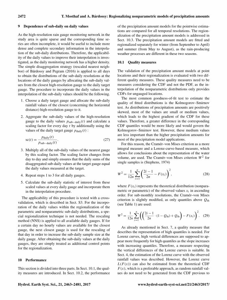
9 Dependence of sub-daily on daily values

As the high-resolution rain gauge monitoring network in thestudy area is quite sparse and the corresponding time se-ries are often incomplete, it would be useful to include moredense and complete secondary information in the interpola-tion of the sub-daily distributions. Therefore, the applicabil-ity of the daily values to improve their interpolation is inves-tigated, as the daily monitoring network has a higher density.The simple disaggregation strategy (rescaled nearest neigh-bor) of Bárdossy and Pegram (2016) is applied to all daysto obtain the distributions of the sub-daily resolutions at thelocations of the daily gauges by allocating the sub-daily val-ues from the closest high-resolution gauge to the daily targetgauge. The procedure to incorporate the daily values in theinterpolation of the sub-daily values should be the following.

1. Choose a daily target gauge and allocate the sub-dailyrainfall values of the closest (concerning the horizontaldistance) high-resolution gauge to it.

2. Aggregate the sub-daily values of the high-resolutiongauge to the daily values psub−daily(t) and calculate ascaling factor for every day t by additionally using thevalues of the daily target gauge pdaily(t) :

sc(t)=pdaily(t)

psub−daily(t). (27)

3. Multiply all of the sub-daily values of the nearest gaugeby this scaling factor. The scaling factor changes fromday to day and simply ensures that the daily sums of thedisaggregated sub-daily values at the target gauge equalthe daily values measured at the target.

4. Repeat steps 1 to 3 for all daily gauges.

5. Calculate the sub-daily statistic of interest from thesescaled values at every daily gauge and incorporate themin the interpolation procedure.

The applicability of this procedure is tested with a cross-validation, which is described in Sect. S3. For the incorpo-ration of the daily values within the regionalization of theparametric and nonparametric sub-daily distributions, a spe-cial regionalization technique is not needed. The rescalingmethod (NNS) is applied to all available daily gauges. If fora certain day no hourly values are available for the closestgauge, the next closest gauge is used for the rescaling ofthat day in order to increase the sub-daily sample size at thedaily gauge. After obtaining the sub-daily values at the dailygauges, they are simply treated as additional control pointsfor the regionalization.

10 Performance

This section is divided into three parts. In Sect. 10.1, the qual-ity measures are introduced. In Sect. 10.2, the performance

of the precipitation amount models for the pointwise estima-tions are compared for all temporal resolutions. The region-alization of the precipitation amount models is addressed inSect. 10.3. The precipitation amount models are fitted andregionalized separately for winter (from September to April)and summer (from May to August), as the rain-producingweather processes are different in these two seasons.

10.1 Quality measures

The validation of the precipitation amount models at pointlocations and their regionalization is evaluated with two dif-ferent quality measures. These quality measures need to bemeasures considering the CDF and not the PDF, as the in-terpolation of the nonparametric distributions only providesCDFs for ungauged locations.

The most common goodness-of-fit test to estimate thequality of fitted distributions is the Kolmogorov–Smirnovtest. As distributions of precipitation amounts are positivelyskewed, most of the values are small or medium values,which leads to the highest gradient of the CDF for thesevalues. Therefore, a greater difference in the correspondingCDF quantiles would be more likely and would govern theKolmogorov–Smirnov test. However, these medium valuesare less important than the higher precipitation amounts formost of the precipitation model applications.

For this reason, the Cramér–von Mises criterion as a moreintegral measure and a Lorenz-curve-based measure, whichallows for conclusions about the representation of the watervolume, are used. The Cramér–von Mises criterion W 2 forsingle samples is (Stephens, 1974)

W 2=

112n

n∑i=1

(2i− 1

2n−F(xi)

)2

, (28)

where F(xi) represents the theoretical distribution (nonpara-metric or parametric) of the observed values xi in ascendingorder. For sub-monthly resolutions, the Cramér–von Misescriterion is slightly modified, as only quantiles above Qth(see Table 1) are used:

W 2=

112n

n∑i=1

((2i− 1

2n· (1−Qth)+Qth

)−F(xi)

)2

. (29)

As already mentioned in Sect. 7, a quality measure thatdescribes the representation of high quantiles is needed. ForLorenz curves, high vertical differences are supposed to ap-pear more frequently for high quantiles as the slope increaseswith increasing quantiles. Therefore, a measure respectingthe vertical differences of the Lorenz curves is suitable. InSect. 4, the estimation of the Lorenz curve with the observedrainfall values was described. However, the Lorenz curveL(F(x)) can also be estimated from the theoretical CDFF(x), which is a preferable approach, as random rainfall val-ues do not need to be generated from the CDF previous to



Table 3. The mean and median of the two quality measuresW2 andLd for the 10 precipitation amount models over the study region forhourly values (1 h) in the winter season. The bold numbers indicatethe lowest (best) value of the corresponding measure.

W2 Ld

Mean Median Mean Median

P-Exp-MLM 0.009718 0.008104 0.2399 0.2004P-Gamma-MLM 0.00263 0.002146 0.0752 0.04835P-Mixed-Exp-MLM 0.0007967 0.0004331 0.02026 0.007648P-Pareto-MLM 0.0006701 0.0003277 0.008036 0.001959P-Weibull-MLM 0.001578 0.0012 0.03891 0.02249

P-Gamma-MOM 0.03089 0.01897 0.1656 0.04182P-Pareto-MOM 0.001074 0.0005668 0.004482 0.002213P-Weibull-MOM 0.01418 0.00827 0.08677 0.04182

NP-SRT 0.0003752 0.0001995 0.01815 0.01448NP-SJ 0.0003485 0.0001954 0.01492 0.01156

the Lorenz curve estimation:

L(F(x))=

∫ F0 x(F )dF∫ 10 x(F )dF

, (30)

where x(F ) is the gauge-wise quantile function (the inverseof the CDF). The integrals of the quantile functions areestimated numerically, because the nonparametrically esti-mated distribution functions are not analytically invertible.The Lorenz curve criterion Ld used here is the squared dif-ference of the observed L(Fn(x)) and the modeled Lorenzcurve L(F(x)):

Ld =

n∑i=1(L(Fn(x))−L(F(x)))

2. (31)

The differences in the Lorenz curves are only estimated forvalues greater than QVth (see Table 1). Within the validationof the regionalization, only the values above the highest QVthamong the observed and regionalized values for each gaugeare evaluated, as they may differ for the different techniques.

10.2 Point models

To determine an overall performance ranking for the remain-ing models, the arithmetic mean and the median over thenumber of gauges for both measures of quality (the Cramér–von Mises criterion W 2 and the Lorenz curve criterion Ld)are first calculated for each precipitation amount model. Thisleads to four different measures, which are shown for hourlyvalues in the winter season in Table 3. Note that the meanvalues reflect the robustness and the median values representa good average performance of one precipitation model forthe whole study region.

To combine the four statistics (the mean and median ofW 2

and Ld, respectively) into one single performance measure,every value in Table 3 is then divided by the smallest (best)

value (the bold numbers) of its corresponding quality mea-sures, indicating the relative performance with respect to thebest model. This leads to one number for each statistic andprecipitation model starting from 1 for the best-performingmodel for each statistic. The bigger this number, the worseits relative performance. These four numbers are then addedtogether, which results in a single number for each precipi-tation amount model to define the performance ranking foreach temporal resolution. A ranking number of 4 is the low-est possible number and implies that the related model showsthe best performance for all four quality measures. In Ta-ble 4, the ranking numbers for all temporal resolutions andboth seasons are shown.

With the ranking numbers, the best-performing precipita-tion amount model is estimated for each season and tempo-ral resolution. Among the nonparametric methods (NP), Sil-verman’s rule of thumb (SRT) and the plug-in approach ofSheather and Jones (1991) (SJ) show very similar results.The generalized Pareto distribution with an MLM parame-ter estimation (Pareto-MLM) exhibits the best performanceamong the (P) parametric models for the hourly resolution.The mixed-exponential distribution with an MLM parame-ter estimation (Mixed-Exp-MLM) leads to the best resultsfor the remaining sub-daily and daily resolutions. For tempo-ral resolutions greater than 1 d the Weibull distribution witha MOM parameter estimation (Weibull-MOM) leads to thebest results, except for the daily resolution in the winter sea-son, where the Pareto-MOM combination is better. The bestperformance of the Weibull distribution for the monthly val-ues coincides with the results of Beck (2013) for the samestudy region.

The performance ranking of the different methods is quitesimilar in winter and summer. The nonparametric methodsalways lead to better performances concerning the Cramér–von Mises criterion W 2. The parametric estimations lead tobetter results regarding the Lorenz curve criterion Ld (for de-tails, see Tables S2 and S3). Figure 6 may provide an ex-planation for the differences in performance regarding thesetwo quality measures. The graphs show the CDFs and Lorenzcurves for the hourly (1 h) and 12-hourly (12 h) resolution fora chosen gauge. For the hourly resolution, the nonparamet-ric SRT method leads to better results for both measures. Anequally good performance regarding theW 2 for the paramet-ric and nonparametric method can be observed for the 12-hourly resolution. However, the nonparametric method per-forms worse regarding the Ld measure, as it overestimatesthe water volume represented by the higher quantiles. Thereason for this can already be observed in the CDF, wherethe nonparametric method systematically overestimates thevalues of the high quantiles. The parametric method can leadto overestimations and underestimations. This influences theW 2 criterion in the same way as a constant overestimation(see the squared differences in Eq. 28), but it seems to leadto better results regarding the Ld criterion.



Table 4. The performance ranking numbers of the precipitation amount models for the pointwise estimations. The underlined numbersindicate the best parametric (P) and nonparametric (NP) models. The bold numbers indicate the best overall model.

Winter season

1 h 2 h 3 h 6 h 12 h 1 d 5 d m

P-Exp-MLM 225.18 145.85 129.44 69.16 37.67 41.63 14.60 742.32P-Gamma-MLM 59.99 30.67 22.79 10.43 6.98 11.51 9.03 13.23P-Mixed-Exp-MLM 12.93 5.72 5.38 5.09 4.79 5.15 15.65 742.67P-Pareto-MLM 6.39 6.12 7.29 7.09 6.38 6.40 6.19 978.92P-Weibull-MLM 30.83 14.01 9.74 5.75 4.93 7.51 6.45 24.33

P-Gamma-MOM 265.89 138.15 94.77 41.47 20.24 23.48 6.64 5.50P-Pareto-MOM 8.11 8.8 10.23 9.25 7.96 8.08 5.71 51.16P-Weibull-MOM 123.72 61.72 44.64 21.28 12.37 13.71 5.82 5.11

NP-SRT 13.54 22.06 35.43 42.16 36.22 31.21 17.33 12.40NP-SJ 11.23 22.12 33.82 43.21 38.15 29.15 16.77 17.35

Summer season

1 h 2 h 3 h 6 h 12 h 1 d 5 d m

P-Exp-MLM 245.24 233.50 188.82 70.63 26.14 25.83 21.67 850.52P-Gamma-MLM 51.51 40.53 30.14 12.82 7.43 7.98 10.00 7.22P-Mixed-Exp-MLM 10.37 5.93 5.31 4.71 4.77 4.79 23.10 850.52P-Pareto-MLM 7.58 13.44 12.79 7.13 5.55 5.58 6.67 709.69P-Weibull-MLM 21.08 13.92 10.42 6.63 5.48 6.02 6.61 25.62

P-Gamma-MOM 289.15 145.27 87.73 33.09 15.51 13.44 6.45 7.27P-Pareto-MOM 16.48 14.46 11.55 7.28 5.99 6.08 5.82 47.81P-Weibull-MOM 98.40 51.03 35.23 16.38 9.91 8.48 5.46 5.05

NP-SRT 6.15 19.05 31.54 37.41 36.15 30.76 19.00 9.27NP-SJ 6.91 22.09 36.11 46.41 41.17 33.14 17.64 12.32

The parameter estimation through MOM in combinationwith the Weibull distribution performs better for the higheraggregations, which exhibit more symmetric distributions.For the daily and sub-daily aggregations, the MLM param-eter estimation in combination with the mixed-exponentialdistribution mostly leads to the best results.

The overall performance is best with the mixed-exponential distribution for temporal resolutions between 2hours (2 h) and 1 day (1 d) in both seasons. For the hourlydistribution (1 h), the nonparametric models show the bestoverall performance in the summer season and the third-best performance after the generalized Pareto (Pareto-MLMand Pareto-MOM) distribution in the winter season. For themonthly resolution (m), the Weibull distribution exhibits thebest overall performance in both seasons. For the 5-daily res-olution, the MOM estimation provides the best result in win-ter (Pareto-MOM) and summer (Weibull-MOM).

10.3 Regionalization

In order to estimate the quality of the regionalized precipi-tation amount models, a 2-fold cross-validation (split sam-pling) is used. Two equally sized samples of observation

points are randomly generated (Fig. 7). The simplest region-alization method is using the estimates of the nearest neigh-bor (NN) in the calibration set, which are therefore used asbenchmarks for the quality of the regionalization procedure.Additionally, the daily rescaled nearest neighbors (NNS) areused as a benchmark. In this case, all daily gauges are usedfor the rescaling except for the daily observations at the lo-cations of the respective validation sample.

Following the results of the pointwise estimation in theprevious section, only the Weibull-MOM and the Mixed-Exp-MLM models among the parametric models are investi-gated for the regionalization, as they show good performancefor differing aggregations. They are both investigated for allaggregations to test the difference for interpolated momentsor parameters, except for the monthly aggregation, for whichonly the Weibull distribution is investigated. In order to re-gionalize the Weibull-MOM model, the mean and standarddeviation are spatially interpolated. For the regionalizationof the Mixed-Exp-MLM model, the parameters λ1 and λ2are interpolated, while its parameter α is kept constant forthe whole study region.

As the two nonparametric approaches SRT and SJ showvery similar results during the pointwise estimation, only



0 5 10 15 20 25 30 35

Precipitation (mm)

0.95

0.96

0.97

0.98

0.99

1.00

F(-

)

Data

srt (W 2: 0.0004)

Mixed-exp (W 2: 0.0008)

0.95 0.96 0.97 0.98 0.99 1.00

Quantiles (F (-))

0.2

0.3

0.4

0.5

0.6

0.7

0.8

0.9

1.0

Cum

ula

tive sh

are of

wat

er v

olum

e (-

)

Data

srt (Ld: 0.0442)

Mixed-exp (Ld: 0.0718)

(a) 1h

0 10 20 30 40

Precipitation (mm)

0.86

0.88

0.90

0.92

0.94

0.96

0.98

1.00

F(-

)

Data

srt (W 2: 0.0010)

Mixed-exp (W 2: 0.0010)

0.86 0.88 0.90 0.92 0.94 0.96 0.98 1.00

Quantiles (F (-))

0.2

0.3

0.4

0.5

0.6

0.7

0.8

0.9

1.0

Cum

ula

tive sh

are of w

ater

vol

um

e (-

)

Data

srt (Ld: 0.2166)

Mixed-exp (Ld: 0.0102)

(b) 12h

Figure 6. Empirical (data), nonparametric (SRT) and parametric (Mixed-Exp) CDF and Lorenz curve examples for the hourly (1 h, a) and12-hourly (12 h, b) resolution of a chosen gauge. The values of the two quality measures Ld and W2 are also indicated.

Figure 7. The locations of the two 2-fold cross-validation samples for the sub-daily (a) and daily gauges (b).

the SRT approach is interpolated. For the regionalization ofthe nonparametric model, the QVc values (see Table 2 andEq. 25) are used to estimate the interpolation weights, whichare further applied to the remaining quantiles. Following theconclusions in Sect. 9, the daily gauges can be used to set up

distribution functions for the sub-daily values with a scalednearest neighbor approach (NNS).



Figure 8. Illustrations for the kriging procedure of the nonparametric distributions with the daily values (1 d) in the summer season usingcalibration sample 1 (see Fig. 7). The (a) nonparametric QVc ofQc = 0.865 at the gauges, which then lead to the interpolated values (b) usingthe interpolation weights φj resulting from PK. The same interpolation weights φj are used for the remaining quantiles, for which exampleresults are shown for the quantiles (c) F= 0.72 and (d) F= 0.98. An exponential variogram with a range of 41 km and a sill of 2.2 mm2 isused.

10.3.1 Variogram estimation

The first step during the regionalization procedure is the esti-mation of the theoretical variograms. The interpolation vari-ables of the three precipitation amount models, for which the-oretical variograms need to be estimated for the two seasonsand eight temporal resolutions, are as follows.

1. P-Mixed-Exp-MLM: λ1, λ1.

2. P-Weibull-MOM: mean, standard deviation.

3. NP-SRT: QVc values (see Table 2 and Eq. 25).

During the estimation of the parameters of the Weibull dis-tribution with MOM, QVth is subtracted from the rainfallvalues prior to the estimation of the mean and the standarddeviation. As the mean of these values shows lower spatialdependencies than the mean of the censored values withoutsubtraction, QVth is added to the mean values of the parame-ter estimation before the regionalization. After the regional-ization, they are subtracted again to determine the parameters

of the Weibull distribution. The variogram models are alsofitted to QVth, as the corresponding values serve as startingpoints for the parametric models at the ungauged locations.Figures S4 to S7 in the Supplement show example theoreticalvariograms for the different parameters for temporal resolu-tions of 1 and 12 h for the winter and summer seasons ofcalibration sample 2.

It is difficult to compare the spatial persistence of T (seeFig. 3) with the spatial persistence of the different distribu-tion parameters (see Figs. S4 to S7), as T considers the wholedistribution function and the distribution parameters only de-scribe the properties of the distribution. However, the rangeof T was about 35 km, which can also be observed for someof the parameters, especially the mean of P-Weibull-MOM,the QVc of NP-SRT and QVth.

10.3.2 Precipitation amount models

The regionalization of the precipitation amount models isevaluated with the same quality measures as the pointwise es-



Table 5. The performance ranking numbers for the 2-fold cross-validation of the regionalized precipitation amount models in the winterseason. The underlined numbers indicate the best parametric (P) and nonparametric (NP) models. The bold numbers indicate the best overallmodel for each validation sample and temporal resolution.

Calibration sample 1

1 h 2 h 3 h 6 h 12 h 1 d 5 d m

OK-MOM 10.08 9.85 9.62 6.95 6.36 4.56 4.37 4.14OK-MLM 7.04 7.22 7.11 10.52 6.70 7.60 6.35 –OK-MOM DAILY 7.45 5.97 5.72 4.21 5.32 – – –OK-MLM DAILY 4.46 4.05 4.02 4.07 4.39 – – –

PK-NP 7.18 8.21 8.94 8.98 9.21 5.56 7.24 6.94PK-NP DAILY 4.09 5.74 6.00 5.68 10.09 – – –

NNS-MOM 7.59 6.76 6.73 5.79 7.01 – – –NN-MOM 13.78 13.27 13.68 10.45 9.85 6.05 6.09 6.48NNS-MLM 6.48 5.88 6.44 5.61 5.69 – – –NN-MLM 10.04 9.81 10.39 10.19 10.51 5.41 7.40 288.07NNS-NP 5.82 7.09 7.75 7.27 11.53 – – –NN-NP 10.65 12.22 13.19 13.10 13.81 7.65 9.03 9.76


1 h 2 h 3 h 6 h 12 h 1 d 5 d m


PK-NP 5.67 8.37 10.86 11.70 9.54 6.37 9.73 7.59PK-NP DAILY 4.14 6.00 7.49 8.49 11.15 – – –


timation, the Cramér–von Mises criterionW 2 and the Lorenzcurve criterion Ld. The investigated interpolation approachesfor the parametric distributions are listed in the following.

1. OK-MOM: OK of the Weibull distribution fitted withMOM.

2. OK-MLM: OK of the mixed-exponential distributionfitted with MLM.

3. OK-MOM Daily: OK of the Weibull distribution includ-ing the scaled NNS values of the daily gauges (only forthe sub-daily aggregations).

4. OK-MLM Daily: OK of the mixed-exponential distribu-tion including the scaled NNS values of the daily gauges(only for the sub-daily aggregations).

The interpolation approaches for the nonparametric mod-els are as follows.

1. PK-NP: PK of the nonparametric models, which are es-timated using SRT.

2. PK-NP Daily: PK of the nonparametric models includ-ing the scaled NNS values of the daily gauges (only forthe sub-daily aggregations).

In Fig. 8, parts of the interpolation procedure for PK-NPare shown for the daily aggregation; the nonparametric QVcat the calibration gauges and three interpolation fields areshown.

In Tables 5 and 6, the performance ranking numbers of theregionalized precipitation amount models are summarizedfor the winter season and for the summer season. The dif-ferences between the two cross-validation samples are quitesmall, so the performances result not from the positioningof the gauges in the samples, but from the interpolation ap-proaches. Among the parametric methods, the MOM ap-proaches mostly perform better than the MLM approaches



Table 6. The performance ranking numbers for the 2-fold cross-validation of the regionalized precipitation amount models in the summerseason. The underlined numbers indicate the best parametric (P) and nonparametric (NP) models. The bold numbers indicate the best overallmodel for each validation sample and temporal resolution.


1 h 2 h 3 h 6 h 12 h 1 d 5 d m


PK-NP 5.37 10.40 12.16 11.70 9.71 9.83 11.34 5.89PK-NP DAILY 4.30 8.27 9.97 10.42 18.88 – – –



1 h 2 h 3 h 6 h 12 h 1 d 5 d m


PK-NP 5.67 6.82 8.11 8.53 6.62 9.63 9.79 6.99PK-NP DAILY 4.27 7.01 8.30 9.75 13.60 – – –


for aggregations greater than or equal to 1 day during thewinter season. In the summer season, the MOM approachesperform mostly worse than the MLM approaches for ag-gregations smaller than 6 h and vice versa for higher ag-gregations. Interpolating moments, therefore, seems to bemore robust than interpolating parameters of the distribu-tions as the performance ranking changed in favor of theMOM approaches compared to the pointwise results (see Ta-ble 4). Only for the more strongly skewed distributions ofthe smaller aggregations does the MLM approach still out-perform the MOM approach.

Comparing the nonparametric interpolation approacheswith the parametric interpolation approaches shows that thenonparametric approach performs best for hourly (1 h) valuesfor both calibration samples in both seasons. This is in linewith the pointwise estimations, for which the nonparametricapproaches also produced very good results for the hourlyresolution in both seasons.

It is obvious that using the scaled values of the dailygauges is very beneficial, as the approaches incorporat-ing these values almost always include the best-performingmethod, except for the 12 h aggregation in the summer sea-son.

As a benchmark, the interpolation results are also shownfor the parametric and nonparametric estimates of the nearestneighbors (NN) and additionally using scaled daily gaugesfor the sub-daily aggregations (NNS). Among the benchmarkmethods, the NNS approaches perform better than the sim-pler NN approaches for the sub-daily aggregations, exceptfor the 12-hourly (12 h) resolution in summer. Since the bestinterpolation approach almost always, with only three ex-ceptions, performs better than the best nearest neighbor ap-proach, the regionalization of the distributions seems to beworthwhile.



11 Conclusions

Comparing different modeling schemes for the precipitationamounts at point locations (see Table 4) over different tem-poral resolutions has revealed several findings. The nonpara-metric estimates only perform better for the hourly resolutionin the summer season. They have problems, especially in re-producing the volume correctly, as they seem to have difficul-ties with high quantiles. The causes for this deficiency couldbe the numeric interpolation or the small number of rainfallvalues at high quantiles. For temporal resolutions between2 h and 1 month, the parametric distributions outperformthe nonparametric distributions for both seasons. Among theparametric methods, the MLM parameter estimation (Mixed-Exp-MLM and Pareto-MLM) performs better for the sub-daily and daily aggregations, whereas the MOM parameterestimation (Weibull-MOM and Pareto-MOM) has the advan-tage for higher aggregations.

The regionalization of the precipitation amount modelsshowed (see Tables 5 and 6) that the proposed interpola-tion scheme for the nonparametric distributions is useful as itdoes not worsen its performance ranking compared to the es-timation at point locations. Among the parametric methods,the interpolation of moments turned out to be more robustthan the interpolation of parameters. The proposed regional-ization scheme for nonparametric models could also be testedin different research fields whenever nonparametric distribu-tions may provide good representations of pointwise modelsand the order of the quantiles is persistent over spatially dis-tributed locations. Especially for applications in which mul-timodal distributions are common, this interpolation schememay be of great interest because kernel density estimates, incontrast to parametric models, can easily model multimodaldistributions.

As auxiliary variables, the use of daily gauges for sub-daily resolutions is very beneficial, as was suggested by ourdata analysis in Sect. S3 and is also proven by the evaluationof the regionalization.

In general, the regionalization of the distributions seemsto be worthwhile as it nearly always performs better thanthe nearest neighbor (horizontal distance) approaches, whichwould be the simplest estimate. As lower rainfall values wereexcluded from this study due to their minor importance andmeasurement errors, the results are not directly comparableto those of most of the other publications within this researchfield.

The difficulty for nonparametric distributions in represent-ing water volumes may be reduced by using the Epanech-nikov kernel with finite support as proposed by Rajagopalanet al. (1997). However, the use of an Epanechnikov kernelinstead of a Gaussian kernel reduces the ability to model pre-cipitation beyond the range of historical data. Additionally,ways of incorporating elevation within the regionalization ofthe nonparametric distributions need to be tested. Mamalakiset al. (2017) used kriged two-component parametric distribu-

tions (a generalized Pareto distribution for higher, and an ex-ponential distribution for lower daily precipitation amounts)for the bias correction and downscaling of rainfall result-ing from a climate model. They applied a parameter esti-mation through probability-weighted moments, which couldalso be compared to the presented estimation approaches forthe regionalization of distributions on varying temporal res-olutions. Finally, the nonparametric interpolation approachcould also be applied to parametric or empirical distributionsand should be tested for various study regions.

Data availability. The sub-daily precipitation data sets used herewere obtained from the LUBW during various research projects andare not available to the public as far as the authors know. There-fore, they can not be provided by the authors. The daily data setwas downloaded from the WebWerdis homepage (http://www.dwd.de/DE/leistungen/webwerdis/webwerdis.html, DWD, 2017a) of theDWD, for which a personal account is required. However, to theknowledge of the authors any academic researcher can apply for apersonal account, and some of the daily and sub-daily values usedhere also seem to be available on the homepage of the DWD Cli-mate Data Center (http://www.dwd.de/DE/klimaumwelt/cdc/cdc_node.html, DWD, 2017b).

The Supplement related to this article is available onlineat doi:10.5194/hess-21-2463-2017-supplement.

Competing interests. The authors declare that they have no conflictof interest.

Acknowledgements. The work of many people developing differentlibraries in the PYTHON programming language (Jones et al.,2001; van der Walt et al., 2011; McKinney, 2010) made the workon the presented research much more convenient and helped a lotto illustrate (Hunter, 2007) its findings. The authors appreciatethe valuable comments on an earlier draft of the manuscript byGeoffrey Pegram (University of KwaZulu-Natal, Durban, SouthAfrica). Three anonymous reviewers helped a lot to improve thequality of the manuscript. The authors also want to thank theGerman Federal Ministry of Education and Research (BMBF)for funding this work through the funding measure Smart andMultifunctional Infrastructural Systems for Sustainable WaterSupply, Sanitation and Stormwater Management (INIS). Further-more, the authors would like to thank the Environmental Agencyof Baden-Württemberg (LUBW) and the German MeteorologicalService (DWD) for the provision of rainfall data.

Edited by: D. KoutsoyiannisReviewed by: three anonymous referees


http://www.dwd.de/DE/leistungen/webwerdis/webwerdis.html


http://www.dwd.de/DE/klimaumwelt/cdc/cdc_node.html


http://dx.doi.org/10.5194/hess-21-2463-2017-supplement


References

Acreman, M. C.: A simple stochastic model of hourly rainfallfor Farnborough, England, Hydrolog. Sci. J., 35, 119–148,doi:10.1080/02626669009492414, 1990.

Anderson, T. W.: On the Distribution of the Two-Sample Cramer-von Mises Criterion, Ann. Math. Statist., 33, 1148–1159,doi:10.1214/aoms/1177704477, 1962.

Arns, A., Wahl, T., Dangendorf, S., Mudersbach, C., andJensen, J.: Ermittlung regionalisierter Extremwasserstände fürdie Schleswig-Holsteinische Nordseeküste, Hydrologie undWasserbewirtschaftung, HW57, doi:10.5675/HyWa_2013,6_1,http://www.hywa-online.de/ermittlung-regionalisierter-extremwasserstaende-fuer-die-schleswig-holsteinische-nordseekueste/ (last access: 28 April 2017), 2013.

Atkinson, K. E.: An Introduction to Numerical Analysis (2nd ed.),John Wiley & Sons, New York, 1989.

Bárdossy, A.: Generating precipitation time series using sim-ulated annealing, Water Resour. Res., 34, 1737–1744,doi:10.1029/98WR00981, 1998.

Bárdossy, A. and Pegram, G. G. S.: Space-time conditional disag-gregation of precipitation at high resolution via simulation, WaterResour. Res., 52, 920–937, doi:10.1002/2015WR018037, 2016.

Bárdossy, A. and Plate, E. J.: Space-time model for daily rainfallusing atmospheric circulation patterns, Water Resour. Res., 28,1247–1259, doi:10.1029/91WR02589, 1992.

Bárdossy, A., Giese, H., Haller, B., and Ruf, J.: Erzeugung syn-thetischer Niederschlagsreihen in hoher zeitlicher Auflösung fürBaden-Württemberg, Wasserwirtschaft, 90, 548–553, 2000.

Beck, F.: Generation of spatially correlated synthetic rainfall timeseries in high temporal resolution: a data driven approach, PhDthesis, Universität Stuttgart, available at : http://elib.uni-stuttgart.de/opus/volltexte/2013/8216 (last access: 28 April 2017), 2013.

Bowman, A. and Azzalini, A.: Applied Smoothing Techniques forData Analysis: The Kernel Approach with S-Plus Illustrations:The Kernel Approach with S-Plus Illustrations, OUP Oxford,1997.

Bowman, A. W.: An Alternative Method of Cross-Validation forthe Smoothing of Density Estimates, Biometrika, 71, 353–360,doi:10.1093/biomet/71.2.353, 1984.

Buishand, T. A. and Brandsma, T.: Multisite simulation of dailyprecipitation and temperature in the Rhine Basin by nearest-neighbor resampling, Water Resour. Res., 37, 2761–2776,doi:10.1029/2001WR000291, 2001.

Burton, A., Kilsby, C., Fowler, H., Cowpertwait, P., andO’Connell, P.: RainSim: A spatial-temporal stochastic rainfallmodelling system, Environ. Modell. Softw„ 23, 1356–1369,doi:10.1016/j.envsoft.2008.04.003, 2008.

Charpentier, A. and Flachaire, E.: Log-Transform Kernel DensityEstimation of Income Distribution, doi:10.2139/ssrn.2514882,2014.

Chen, J. and Brissette, F.: Stochastic generation of daily precipita-tion amounts: review and evaluation of different models, Clim.Res., 59, 189–206, doi:10.3354/cr01214, 2014.

Chen, S.: Probability Density Function Estimation Us-ing Gamma Kernels, Ann. I. Stat. Math., 52, 471–480,doi:10.1023/A:1004165218295, 2000.

Ciach, G.: Local random errors in tipping-bucket rain gaugemeasurements, J. Atmos. Ocean. Tech., 20, 752–759,

doi:10.1175/1520-0426(2003)20<752:LREITB>2.0.CO;2,2003.

Cohen, A. C.: Maximum Likelihood Estimation in the Weibull Dis-tribution Based on Complete and on Censored Samples, Tech-nometrics, 7, 579–588, doi:10.1080/00401706.1965.10490300,1965.

Duong, T.: ks: Kernel Smoothing, available at: http://CRAN.R-project.org/package=ks (last access: 28 April 2017), r pack-age version 1.10.0, 2015.

DWD (Deutscher Wetterdienst): WebWerdis (Web-based WeatherRequest and Distribution System), available at: http://www.dwd.de/DE/leistungen/webwerdis/webwerdis.html, last access:28 April 2017a.

DWD (Deutscher Wetterdienst): CDC (Climate Data Cen-ter), available at: http://www.dwd.de/DE/klimaumwelt/cdc/cdc_node.html, last access: 28 April 2017b.

Giraldo, R., Delicado, P., and Mateu, J.: Ordinary kriging forfunction-valued spatial data, Environ. Ecol. Stat., 18, 411–426,doi:10.1007/s10651-010-0143-y, 2011.

Goulard, M. and Voltz, M.: Geostatistical Interpolation of Curves:A Case Study in Soil Science, 805–816, Springer, Netherlands,Dordrecht, doi:10.1007/978-94-011-1739-5_64, 1993.

Haberlandt, U.: Stochastic Rainfall Synthesis Using Region-alized Model Parameters, J. Hydrol. Eng., 3, 160–168,doi:10.1061/(ASCE)1084-0699(1998)3:3(160), 1998.

Habib, E., Krajewski, W., and Kruger, A.: Sampling errors oftipping-bucket rain gauge measurements, J. Hydrol. Eng., 6,159–166, doi:10.1061/(ASCE)1084-0699(2001)6:2(159), 2001.

Harrold, T. I., Sharma, A., and Sheather, S. J.: A nonparametricmodel for stochastic generation of daily rainfall occurrence, Wa-ter Resour. Res., 39, doi:10.1029/2003WR002182, 2003.

Hosking, J. R. M. and Wallis, J. R.: Parameter and Quantile Estima-tion for the Generalized Pareto Distribution, Technometrics, 29,339–349, doi:10.2307/1269343, 1987.

Hunter, J. D.: Matplotlib: A 2D Graphics Environment, Comput.Sci. Eng., 9, 90–95, doi:10.1109/MCSE.2007.55, 2007.

Jones, E., Oliphant, T., Peterson, P., et al., SciPy: Open source sci-entific tools for Python, available at: http://www.scipy.org/ (lastaccess: 28 April 2017), 2001.

Jones, M. C., Marron, J. S., and Sheather, S. J.: A brief survey ofbandwidth selection for density estimation, J. Am. Stat. Assoc.,91, 401–407, 1996.

Katz, R. W. and Parlange, M. B.: Generalizations of Chain-Dependent Processes: Application to Hourly Precipitation, WaterResour. Res., 31, 1331–1341, doi:10.1029/94WR03152, 1995.

Kitanidis, P. K.: Introduction to geostatistics: Application to hydro-geology, Cambridge University Press, 1997.

Kleiber, W., Katz, R. W., and Rajagopalan, B.: Daily spa-tiotemporal precipitation simulation using latent and trans-formed Gaussian processes, Water Resour. Res., 48, 1–17,doi:10.1029/2011WR011105, 2012.

Lall, U., Rajagopalan, B., and Tarboton, D. G.: A nonparametricwet/dry spell model for resampling daily precipitation, Water Re-sour. Res., 32, 2803–2823, doi:10.1029/96WR00565, 1996.

Landesanstalt für Umwelt, Messungen und Naturschutz Baden-Württemberg (LUBW): Klimaatlas Baden-Württemberg,available at: http://www4.lubw.baden-wuerttemberg.de/servlet/is/244295/ (last access: 28 April 2017), 2006.


http://dx.doi.org/10.1080/02626669009492414

http://dx.doi.org/10.1214/aoms/1177704477

http://dx.doi.org/10.5675/HyWa_2013,6_1

http://www.hywa-online.de/ermittlung-regionalisierter



http://dx.doi.org/10.1029/98WR00981

http://dx.doi.org/10.1002/2015WR018037


http://elib.uni-stuttgart.de/opus/volltexte/2013/8216

http://elib.uni-stuttgart.de/opus/volltexte/2013/8216

http://dx.doi.org/10.1093/biomet/71.2.353

http://dx.doi.org/10.1029/2001WR000291

http://dx.doi.org/10.1016/j.envsoft.2008.04.003

http://dx.doi.org/10.2139/ssrn.2514882

http://dx.doi.org/10.3354/cr01214

http://dx.doi.org/10.1023/A:1004165218295

http://dx.doi.org/10.1175/1520-0426(2003)20<752:LREITB>2.0.CO;2

http://dx.doi.org/10.1080/00401706.1965.10490300

http://CRAN.R-project.org/package=ks

http://CRAN.R-project.org/package=ks





http://dx.doi.org/10.1007/s10651-010-0143-y

http://dx.doi.org/10.1007/978-94-011-1739-5_64

http://dx.doi.org/10.1061/(ASCE)1084-0699(1998)3:3(160)

http://dx.doi.org/10.1061/(ASCE)1084-0699(2001)6:2(159)

http://dx.doi.org/10.1029/2003WR002182

http://dx.doi.org/10.2307/1269343

http://dx.doi.org/10.1109/MCSE.2007.55

http://www.scipy.org/


http://dx.doi.org/10.1029/2011WR011105


http://www4.lubw.baden-wuerttemberg.de/servlet/is/244295/

http://www4.lubw.baden-wuerttemberg.de/servlet/is/244295/


Lawson, C. and Hanson, R.: Solving Least Squares Problems,SIAM, 1987.

Li, C., Singh, V. P., and Mishra, A. K.: Simulation of the entire rangeof daily precipitation using a hybrid probability distribution, Wa-ter Resour. Res., 48, doi:10.1029/2011WR011446, 2012.

Lorenz, M. O.: Methods of Measuring the Concentration of Wealth,Publ. Am. Stat. Assoc., 9, 209–219, doi:10.2307/2276207, 1905.

Mamalakis, A., Langousis, A., Deidda, R., and Marrocu, M.: Aparametric approach for simultaneous bias correction and high-resolution downscaling of climate model rainfall, Water Resour.Res., 53, 2149–2170, doi:10.1002/2016WR019578, 2017.

McKinney, W.: Data Structures for Statistical Computing in Python,in: Proceedings of the 9th Python in Science Conference, editedby: van der Walt, S. and Millman, J., 51–56, 2010.

McMillan, H., Krueger, T., and Freer, J.: Benchmarking ob-servational uncertainties for hydrology: rainfall, river dis-charge and water quality, Hydrol. Process., 26, 4078–4111,doi:10.1002/hyp.9384, 2012.

Menafoglio, A., Secchi, P., and Dalla Rosa, M.: A Universal Krig-ing predictor for spatially dependent functional data of a HilbertSpace, Electron. J. Statist., 7, 2209–2240, doi:10.1214/13-EJS843, 2013.

Menafoglio, A., Guadagnini, A., and Secchi, P.: Stochastic simula-tion of soil particle-size curves in heterogeneous aquifer systemsthrough a Bayes space approach, Water Resour. Res., 52, 5708–5726, doi:10.1002/2015WR018369, 2016.

Nystuen, J., Proni, J., Black, P., and Wilkerson, J.: A comparisonof automatic rain gauges, J. Atmos. Ocean. Tech., 13, 62–73,doi:10.1175/1520-0426(1996)013<0062:ACOARG>2.0.CO;2,1996.

Papalexiou, S. M. and Koutsoyiannis, D.: Entropy based derivationof probability distributions: A case study to daily rainfall, Adv.Water Resour., 45, 51–57, doi:10.1016/j.advwatres.2011.11.007,2012.

Pardo-Iguzquiza, E. and Chica-Olmo, M.: Geostatistics with theMatern semivariogram model: A library of computer programsfor inference, kriging and simulation, Comput. Geosci., 34,1073–1079, doi:10.1016/j.cageo.2007.09.020, 2008.

Peel, S. and Wilson, L. J.: Modeling the Distribution of Precipita-tion Forecasts from the Canadian Ensemble Prediction SystemUsing Kernel Density Estimation, Weather Forecast., 23, 575–595, doi:10.1175/2007WAF2007023.1, 2008.

R Core Team: R: A Language and Environment for StatisticalComputing, R Foundation for Statistical Computing, Vienna,Austria, availabale at: https://www.R-project.org/ (last access:28 April 2017), 2015.

Rajagopalan, B., Lall, U., and Tarboton, D. G.: Evaluation of kerneldensity estimation methods for daily precipitation resampling,Journal of Stochastic Hydrology and Hydraulics, 11, 523–547,1997.

Rider, P. R.: The Method of Moments Applied to a Mixture ofTwo Exponential Distributions, Ann. Math. Stat., 32, 143–147,doi:10.1214/aoms/1177705147, 1961.

Sheather, S. J.: Density Estimation, Statist. Sci., 19, 588–597,doi:10.1214/088342304000000297, 2004.

Sheather, S. J. and Jones, M. C.: A Reliable Data-Based BandwidthSelection Method for Kernel Density Estimation, J. Roy. Stat.Soc. B, 53, 683–690, 1991.

Silverman, B. W.: Density estimation for statistics and data analysis,Chapman and Hall, London, 1. publ. edn., 1986.

Stephens, M. A.: EDF Statistics for Goodness of Fit andSome Comparisons, J. Am. Stat. Assoc., 69, 730–737,doi:10.1080/01621459.1974.10480196, 1974.

Szidarovszky, F., Baafi, E. Y., and Kim, Y. C.: Krigingwithout negative weights, Math. Geol., 19, 549–559,doi:10.1007/BF00896920, 1987.

van der Walt, S., Colbert, S. C., and Varoquaux, G.: The NumPy Ar-ray: A Structure for Efficient Numerical Computation, Comput.Sci. Eng., 13, 22–30, doi:10.1109/MCSE.2011.37, 2011.

Wand, M.: KernSmooth: Functions for Kernel Smoothing Support-ing Wand & Jones (1995), available at: http://CRAN.R-project.org/package=KernSmooth (last access: 28 April 2017), r packageversion 2.23-15, 2015.

Wilks, D. S.: Multisite generalization of a daily stochasticprecipitation generation model, J. Hydrol., 210, 178–191,doi:10.1016/S0022-1694(98)00186-3, 1998.

Wilks, D. S.: High-resolution spatial interpolation of weather gen-erator parameters using local weighted regressions, Agr. ForestMeteorol., 148, 111–120, doi:10.1016/j.agrformet.2007.09.005,2008.

Wilks, D. S.: A gridded multisite weather generator and syn-chronization to observed weather data, Water Resour. Res., 45,doi:10.1029/2009WR007902, 2009.

Wilks, D. S. and Wilby, R. L.: The weather generation game: a re-view of stochastic weather models, Prog. Phys. Geog., 23, 329–357, doi:10.1177/030913339902300302, 1999.

Woolhiser, D. A. and Pegram, G. G. S.: Maximum Likeli-hood Estimation of Fourier Coefficients to Describe Sea-sonal Variations of Parameters in Stochastic Daily Precipita-tion Models, J. Appl. Meteor., 18, 34–42, doi:10.1175/1520-0450(1979)018<0034:MLEOFC>2.0.CO;2, 1979.


http://dx.doi.org/10.1029/2011WR011446

http://dx.doi.org/10.2307/2276207

http://dx.doi.org/10.1002/2016WR019578

http://dx.doi.org/10.1002/hyp.9384

http://dx.doi.org/10.1214/13-EJS843

http://dx.doi.org/10.1214/13-EJS843

http://dx.doi.org/10.1002/2015WR018369

http://dx.doi.org/10.1175/1520-0426(1996)013<0062:ACOARG>2.0.CO;2

http://dx.doi.org/10.1016/j.advwatres.2011.11.007

http://dx.doi.org/10.1016/j.cageo.2007.09.020

http://dx.doi.org/10.1175/2007WAF2007023.1

https://www.R-project.org/

http://dx.doi.org/10.1214/aoms/1177705147

http://dx.doi.org/10.1214/088342304000000297

http://dx.doi.org/10.1080/01621459.1974.10480196

http://dx.doi.org/10.1007/BF00896920

http://dx.doi.org/10.1109/MCSE.2011.37

http://CRAN.R-project.org/package=KernSmooth

http://CRAN.R-project.org/package=KernSmooth

http://dx.doi.org/10.1016/S0022-1694(98)00186-3

http://dx.doi.org/10.1016/j.agrformet.2007.09.005

http://dx.doi.org/10.1029/2009WR007902

http://dx.doi.org/10.1177/030913339902300302

http://dx.doi.org/10.1175/1520-0450(1979)018<0034:MLEOFC>2.0.CO;2

http://dx.doi.org/10.1175/1520-0450(1979)018<0034:MLEOFC>2.0.CO;2

regionalizing nonparametric models of precipitation

Documents