1

Regression-Based Utilization Prediction Algorithms: An Empirical Investigation

I. Davis, H. Hemmati, R. Holt, M. Godfrey University of Waterloo

Waterloo, Ontario, Canada N2L 3G1 {ijdavis, hhemmati, holt, migod}@uwaterloo.ca

D. Neuse, S. Mankovskii CA Labs

CA Technologies {Douglas.Neuse, Serge.Mankovskii}@ca.com

Abstract Predicting future behavior reliably and efficiently is vital for systems that manage virtual services; such systems must be able to balance loads within a cloud environment to ensure that service level agreements (SLAs) are met at a reasonable expense. These virtual services while often comparatively idle are occasionally heavily utilized. Standard approaches to modeling system behavior (by analyzing the totality of the observed data, such as regression based approaches) tend to predict average rather than exceptional system behavior and may ignore important patterns of change over time. Consequently, such approaches are of limited use in providing warnings of future peak utilization within a cloud environment. Skewing predictions to better fit peak utilizations, results in poor fitting to low utilizations, which compromises the ability to accurately predict peak utilizations, due to false positives.

In this paper, we present an adaptive approach that estimates, at run time, the best prediction value based on the performance of the previously seen predictions. This algorithm has wide applicability. We applied this adaptive technique to two large-scale real world case studies. In both studies, the results show that the adaptive approach is able to predict low, medium, and high utilizations accurately, at low cost, by adapting to changing patterns within the input time series. This facilitates better proactive management and placement of systems running within a cloud.

Copyright 2013 Ian Davis et al. Permission to copy is hereby granted provided the original copyright notice is reproduced in copies made.

1 Introduction Large collections of computers cooperatively providing distributed services so as to support demand for these services are becoming the norm. Single computers hosting multiple virtual ma-chines are now also common. Parallel computing techniques [20] offer the potential for time con-suming computation to be distributed across mul-tiple machines, thus delivering results from a single computation to the consumer much more rapidly. In each case decoupling of computer software from the underlying hardware, permits greater utilization of the hardware, under more balanced workloads, with improvements in re-sponse times, and dramatic reduction in costs. In addition the ability to replicate services over mul-tiple machines permits greater scalability, com-bined with more robustness than would otherwise be possible.

However, if the demands placed on the hard-

ware by the software exceed the capabilities of the hardware, thrashing will occur, response times will rise, and customer satisfaction will plummet. Therefore it is essential [23, 32] to ensure that software is appropriately provisioned across the available hardware in the short to medium term, and that appropriate levels of hardware and soft-ware are purchased and installed to support the collective future end user requirements in the longer term [15, 24, 29, 30].

Without good forecasts [16], data center man-

agers are often forced to over-configure their pools of resources to achieve required availability, in order to honor service level agreements (SLAs). This is expensive, and can still fail to consistently

2

satisfy SLAs. Absent good forecasts, system management software tends to operate in a reac-tive mode and can become ineffective and even disruptive [25]. In this paper we present modifica-tions to standard prediction techniques, which are better able to predict when utilization of a service will be high. Knowing this it becomes possible to better predict when storms will occur, and so avoid such storms.

2 Motivation

This research [8] is motivated by CA Technolo-gies [6] need to develop industrial autonomous solutions for effectively predicting workload of their  clients’  cloud  services,  both  in  the  short  term  (measured in hours), and in the longer term (measured in months). Good short-term predic-tions permit better adaptive job placement and scheduling, while longer term predictions permit appropriate and financially effective proactive provisioning of resources within the cloud envi-ronment.

We were initially provided with a substantive

body of performance data relating to a single large cloud computing environment. This was running a large number of virtual services over a six month period. In total there were 2,133 independent enti-ties whose performance was being captured every six minutes. These included 1,572 virtual ma-chines and 495 physical machines. The physical machines provided support for 56 VMware hosts. On average 53% of the monitored services were active at any time, with a maximum of 85%. The data captured described CPU workloads, memory usage, disk I/O, and network traffic. This data was each consolidated into average and maximum hourly performance figures, and it was the hourly CPU workload data that our research was predi-cated on.

At least 423 services were dedicated to provid-

ing virtual desktop environments, while the cloud was also proving support for web based services, transaction processing, database support, place-ment of virtual services on hosts, and other ser-vices such as performance monitoring and backup.

As is typically the case in desktop environ-

ments, individual computer utilization varies dra-matically. Much of the time little if any intensive

work is being done on a virtual desktop and the virtual service appears almost idle. However, for any virtual desktop there are periods of intense activity, when CPU, memory, disk I/O, and/or network traffic peaks. Similarly within transac-tion processing environments, there will be a wide variety of behaviors, depending on the overall demand placed on such systems.

In our study, the average utilization across all

these services was at most 20% (except for the weekly activity on Sunday afternoon when aver-age utilization rose to almost 50%), but the max-imum utilization across all services, was almost invariably very close to 100% (Fig. 1).

Figure 1: Cloud utilization over time

The frequency distribution of the utilizations

actually observed, was highly skewed, with 83.5% of the utilizations not exceeding 25%. The exponential utilization curve was approximated by 100*(2-u)13.5 (Fig. 2).

Figure 2: Distribution of utilizations

Given this described data, our challenge was

to resolve how one might reasonably predict in the short term (e.g. within the next hour) the in-frequent occasions when a given service was like-ly to be heavily utilized. Knowing this one can

3

then reserve necessary resources for this heavily utilized service, while also avoiding conflicts with other heavily utilized activities, and the resources they depend on.

In this context, accurate predictions that an

idle service will remain idle most of the time, while very occasionally as consequence being wrong, are useless. What are required are predic-tions that (with a reasonable degree of confidence) indicate when future loads will be high, even if such predictions do not mathematically fit the totality of observed and future data as closely as conventional statistical approaches.

Over a longer time frame (measured in weeks

or months) we wished to be able to accurately predict expected workloads, so that a cloud data center could be appropriately managed. Without such long-term predictions it becomes difficult to ensure in a timely fashion that a computing center is provided with adequate power and hardware, and to predict what the future cost of operating the facilities will be.

3 Related Work

Andreolini et al. proposed using moving averages to smooth the input time series, and then using linear extrapolation on two of the smoothed val-ues to predict the next [3]. Dinda et al. compared the ability of a variety of ARIMA like models to predict futures [9]. Nathuji et al. proposed evalu-ating virtual machines in isolation, and then pre-dicted their behavior when run together using multiple input signals to produce multiple predic-tive outputs using difference equations (exponen-tial smoothing) [24].

Istin et al. divided the time series into multi-

ple series using different sampling steps, obtained predictions from each subseries, and then used neural networks to derive a final prediction [19]. Khan et al. also used multiple time series (but derived from distinct workloads) and hidden Mar-kov models, to discover correlations between workloads that can then be used to predict varia-tions in workload patterns [21].

Huhtal et al. proposed that similarity between

related time series might be discovered by using wavelets [17]. Ganapathi discovered linear map-pings from related information (such as workload

and performance data), which produced maximum correlations between this distinct data, and then exploited the discovered similarities between the input data, before recovering actual predictions through inverting these transformations [14].

Povinelli proposed mapping data points at

fixed temporal lags into n-dimensional phase space, clustering the resulting points on their Eu-clidian distance, and then employing a user speci-fied goal function for each point within a cluster to discover (using genetic programming tech-niques) unknown patterns/clusters strongly pre-dictive of future events deemed interesting [11, 27]. Srinivasan et al. also used genetic algorithms, but translated the time series into substrings, with symbols within the string representing the various types of behavior within the time series [28].

More generally, Nikolov proposed that per-

formance might be understood as consequence of given underlying patterns that determined behav-ior, and clustered observed behavior according to the pattern it was most similar to, using a simple distance metric. Behavior might then be predicted, because of the discovered similarity with an un-derstood behavioral pattern [26]. Magnusson proposed that simple underlying short-term pat-terns be detected and that larger longer term com-posite patterns then be discovered through a hierarchical composition of these simpler patterns recursively [22].

4 Linear Regression

Given the data provided us, we elected to focus on predicting physical and virtual CPU utilizations. For each data series, the observed utilizations ut were partitioned into small intervals in increments of 0.05, and for each such partition the average absolute difference between observed values ut and predicted values pt were obtained. This pro-vides a clear picture of how closely prediction matches observed utilization across the utilization spectrum. Then these averages are themselves averaged across the set of data series.

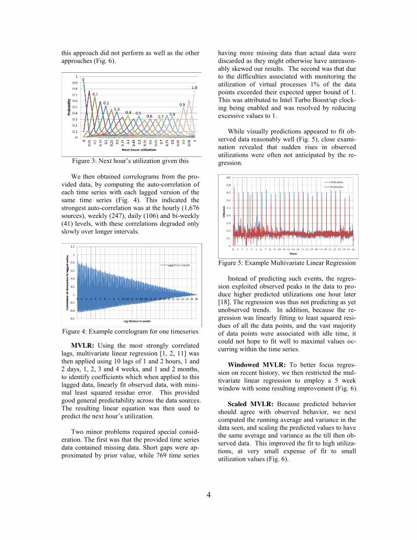
Unchanged: Since there was at least a 30%

probability that utilizations would remain essen-tially unchanged from one hour to the next (Fig. 3), as a trivial baseline measurement we predicted that there would never be change in the utilization observed during the previous hour. As expected

4

this approach did not perform as well as the other approaches (Fig. 6).

Figure 3: Next  hour’s  utilization  given this We then obtained correlograms from the pro-

vided data, by computing the auto-correlation of each time series with each lagged version of the same time series (Fig. 4). This indicated the strongest auto-correlation was at the hourly (1,676 sources), weekly (247), daily (106) and bi-weekly (41) levels, with these correlations degraded only slowly over longer intervals.

Figure 4: Example correlogram for one timeseries

MVLR: Using the most strongly correlated

lags, multivariate linear regression [1, 2, 11] was then applied using 10 lags of 1 and 2 hours, 1 and 2 days, 1, 2, 3 and 4 weeks, and 1 and 2 months, to identify coefficients which when applied to this lagged data, linearly fit observed data, with mini-mal least squared residue error. This provided good general predictability across the data sources. The resulting linear equation was then used to predict  the  next  hour’s  utilization.

Two minor problems required special consid-

eration. The first was that the provided time series data contained missing data. Short gaps were ap-proximated by prior value, while 769 time series

having more missing data than actual data were discarded as they might otherwise have unreason-ably skewed our results. The second was that due to the difficulties associated with monitoring the utilization of virtual processes 1% of the data points exceeded their expected upper bound of 1. This was attributed to Intel Turbo Boost/up clock-ing being enabled and was resolved by reducing excessive values to 1.

While visually predictions appeared to fit ob-

served data reasonably well (Fig. 5), close exami-nation revealed that sudden rises in observed utilizations were often not anticipated by the re-gression.

Figure 5: Example Multivariate Linear Regression

Instead of predicting such events, the regres-

sion exploited observed peaks in the data to pro-duce higher predicted utilizations one hour later [18]. The regression was thus not predicting as yet unobserved trends. In addition, because the re-gression was linearly fitting to least squared resi-dues of all the data points, and the vast majority of data points were associated with idle time, it could not hope to fit well to maximal values oc-curring within the time series.

Windowed MVLR: To better focus regres-

sion on recent history, we then restricted the mul-tivariate linear regression to employ a 5 week window with some resulting improvement (Fig. 6).

Scaled MVLR: Because predicted behavior

should agree with observed behavior, we next computed the running average and variance in the data seen, and scaling the predicted values to have the same average and variance as the till then ob-served data. This improved the fit to high utiliza-tions, at very small expense of fit to small utilization values (Fig. 6).

5

Figure 6: Multivariate Regression Strategies

Weighted MVLR: Because the overall distri-

bution of utilizations was observed to be exponen-tial (Fig. 2) it is reasonable to weight [12] within the regression summations each data point. We employed exponential weighting, in which a data point having utilization u as well as all lags asso-ciated with this data point were multiplied by (1+u)c. This naturally assigned higher utilizations a significantly greater weight, thus skewing the predictions towards higher values, while simulta-neously bounding them by the highest values (Fig. 7). As can be seen a value of c=12 provided the most consistent average absolute error [5] across all of the data sources.

Figure 7: Weighting Regression by (1+u)c

Power MVLR: An alternative to internal

weighting was to presented as input values to the multivariate linear regression uc, rather than u. The final prediction obtained from this modified regression, was then recovered by taking the cth root of the value obtained by the regression.

As an informal justification for this approach,

consider a set of non-negative points ai with 1≤i≤n. The  average  of  this  set  of  points  is  Σai/n. Apply-ing the above transformation for c=2, gives a re-vised  average  value  of  √(  Σai

2/n). The difference

of the square of the revised value to the square of the actual average is simply the variance in the sample.

Since the variance cannot be negative, and

neither can our summations, this implies that the revised average can be no smaller than the origi-nal average, and can agree only when the variance in the original sample is 0. Further, the revised value must remain less than or equal to the maxi-mal original point, with equality reached again, only if the variance in the original sample is 0.

This argument can be used repeatedly for c=2k

(Table 1), suggesting that the shift towards maxi-mal values in the set examined, is a monotonically increasing function, for increasing values of k. The proposed transformation has minimal impact on collections of small values, but for large varia-tions, the shift upwards is quite dramatic (Fig.8), and does provide a much better fit to high ob-served utilizations, by shifting predictions up-wards, while producing a very poor fit to the majority of observed low observed utilizations.

3 Sample Values

Average of Power MLVR c=1 c=2 c=10 c=20 c=30

0,0.05,0.1 0.05 0.06 0.09 0.09 0.10 0,0.1,0.2 0.10 0.13 0.18 0.19 0.19 0,0.15,0.3 0.15 0.19 0.27 0.28 0.29 0,0.2,0.4 0.20 0.26 0.36 0.38 0.39 0,0.25,0.5 0.25 0.32 0.45 0.47 0.48 0,0.3,0.6 0.30 0.39 0.54 0.57 0.58 0,0.35,0.7 0.35 0.45 0.63 0.66 0.67 0,0.4,0.8 0.40 0.52 0.72 0.76 0.77 0,0.45,0.9 0.45 0.58 0.80 0.85 0.87 0,0.5,1.0 0.50 0.65 0.90 0.95 0.96

Table 1: Examples using power MVLR Similarities clearly exist between the results

observed by weighting (changing the regression algorithm itself), and by raising inputs to powers (changing the inputs to the algorithm). Both pro-vide  the  most  consistent  average  error  when  c≈12.

Across a wide range of parameterization of c

the weighted regression produced a consistently lower average absolute error (Fig. 9), and appears to be the better strategy for predicting large utili-

6

zations (Fig. 10 and 11). It also does not require that input values be between 0 and 1.

Figure 8: Power MVLR for varying powers

Figure 9: Comparison of power .v. weighting

Figure 10: Power .v. weighting for c=12

Figure 11: Power .v. weighting for c=20

5 Seasonality

To achieve good long-term predictions, one must consider not only changing trends, modelled reasonably well by the approaches suggested above, but also longer term seasonal contribu-tions.

Fourier: Fast Fourier transforms [13] were

exploited in an effort to discover obvious cyclic patterns within the data. Strong patterns were observed at the daily and weekly level.

Graphing the summation of the ten sine waves

with the largest amplitudes, which are the terms that describe the most dominant variability within the input data, fit the overall seasonality within the provided data well, but failed to fit the peaks in the data at all well (Fig. 12).

Figure 12: Sample Fourier Fit

We extended this computed transform into the

future and used its value at each given hour to predict, which worked well for small utilizations, but not for large utilizations irrespective of the number of sine waves summed (Fig. 13).

Figure 13: Fourier fit to future data

7

Scaled FT: To account for the terms not in-cluded in the contribution to our prediction, it is reasonable to attempt to scale the Fourier trans-form (FT) to better fit the utilizations.

We do this by applying a linear transformation

to the computed Fourier transform. Let m = min(predicted) and using n=100 to limit issues with individual outliers, we compute ū = E(max n observed utilizations), and p̄ = E(max n predicted). Then where p̄ ≠  m we scale each prediction p us-ing the formula  m  +  (p-m)*(  ū  -  m)/(  p̄-m).

The difference between the scaled Fourier

function, and observed data within one representative data source, scaling using the formula y = 0.145927 + (prediction – 0.145927)* 1.51284 is shown in Figure 14.

Figure 14: Sample residue after scaling FT The scaled FT appears to be a good long-term

predictor of future system performance. There is no systemic weakening of the prediction algo-rithm over time, even though predictions in week 26 are derived from data obtained between three and six months earlier (Fig. 15).

Figure 15: Scaled FT average absolute residue

The regular spikes in utilization once each Sunday afternoon (Fig. 1) are not well handled by the scaled FT [7]. These spikes while modeled by the transform are consistently under-estimated, while (in attempting to fit to these spikes) utiliza-tions immediately before and after to such spikes are consistently over-estimated. This is an inevi-table consequence of attempting to model spikes within the data as the summation of a very small number of sine waves.

Without scaling the average error during the

training period would (by construction of the FT) have been 0, but with scaling predictions exceed-ed utilizations on average by 0.066 during the training period and by 0.062 during the testing period (Fig. 16).

Figure 16: Scaled FT average residue

Using this approach across all data sources

was reasonably effective. Across all of our data sources the average absolute error associated with using a Fourier transform to predict future behaviour was almost halved for large utilizations when the Fourier transform was suitably scaled (Fig 17).

Figure 17: Multivariate regression strategies

8

MVLR was a better predictor than scaled FT alone, as was weighted MVLR for high utilizations, but using the scaled FT to predict future seasonality was competitive with linear regression, and remained so over much longer time frames measured not in hours but in months. This is exciting since long-term prediction is inherently difficult.

The most significant drawback of using

Fourier transforms is that unlike regression which could quickly start providing predictions from initially observed results, a substantial amount of prior data must be available, in order to discover seasonality within an input time series. In practice it is proposed that early predictions are predicated on regression alone, while periodically as sufficient data becomes available a fast Fourier transform is employed to repeatedly discover seasonality with the input data.

In general, one cannot assume that seasonal

behaviour of machines within a cloud will remain sufficiently static to provide such long-term predictability. And clearly, further improvement in predictions may be achieved by developing a hybrid algorithm that exploits both Fourier transforms and linear regression simultaneously.

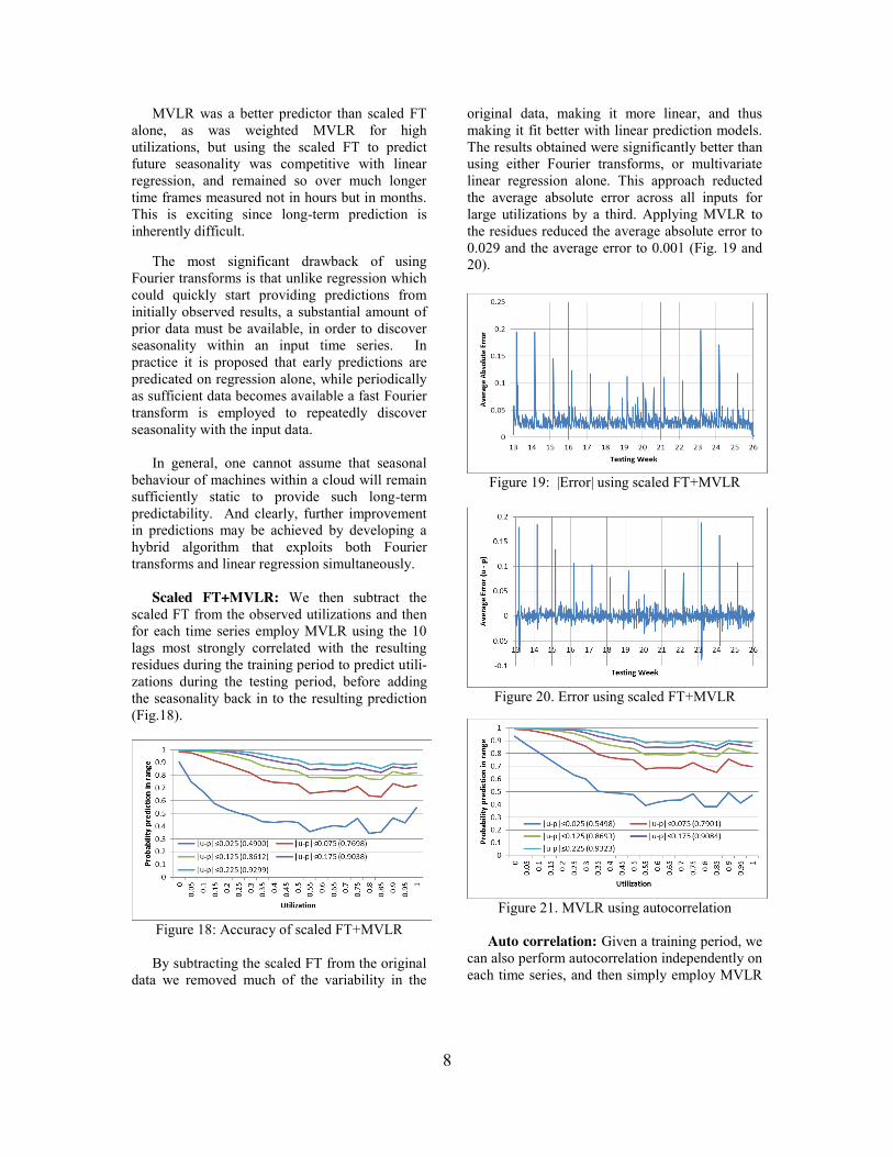
Scaled FT+MVLR: We then subtract the

scaled FT from the observed utilizations and then for each time series employ MVLR using the 10 lags most strongly correlated with the resulting residues during the training period to predict utili-zations during the testing period, before adding the seasonality back in to the resulting prediction (Fig.18).

Figure 18: Accuracy of scaled FT+MVLR By subtracting the scaled FT from the original

data we removed much of the variability in the

original data, making it more linear, and thus making it fit better with linear prediction models. The results obtained were significantly better than using either Fourier transforms, or multivariate linear regression alone. This approach reducted the average absolute error across all inputs for large utilizations by a third. Applying MVLR to the residues reduced the average absolute error to 0.029 and the average error to 0.001 (Fig. 19 and 20).

Figure 19: |Error| using scaled FT+MVLR

Figure 20. Error using scaled FT+MVLR

Figure 21. MVLR using autocorrelation

Auto correlation: Given a training period, we

can also perform autocorrelation independently on each time series, and then simply employ MVLR

9

using the 10 lags most strongly correlated during the training period, to predict utilizations during the testing period. This approach, produced results comparable to using scaled FT+MVLR, but did not perform quite as well for large utilizations. (Fig. 17 and 21).

Adaptive: Rather than exploit a single predic-

tion algorithm, it is possible to use two or more very different prediction algorithms, and decide at runtime which of the provided predictions is most likely to approximate the next utilization we wish to estimate.

A simple approach at time t given predictor’s  

pt and qt is to use single exponential smoothing to weight (using β) the effectiveness of the two pre-dictors. Initially and whenever pt = qt let β =0.5. Otherwise having observed the utilization ut, solve β*pt+(1- β)*qt=ut, set β=max(min(B,1),0), and then use this formula with the next predic-tions to estimate the next utilization. Informally, this next uses whichever algorithm best predicted the observed utilization this time, and interpolates between the next two predictors when the current predictors lie opposite sides of the observed utili-zation.

Figure 22: |Error| using adaptive algorithm

Figure 23: Error using adaptive algorithm

For large utilizations weighted regression re-mains a better predictor than any of the other pre-diction mechanisms. Adaptively using scaled FT+MVLR, together with weighted regression produced an algorithm which outperformed either of these individual algorithms while ensuring a much better fit (|utilization-prediction|) to the peak utilizations observed (Fig. 22 through 25).

Figure 24: Accuracy of algorithm for |u-p|≤0.025

Figure 25: Accuracy of algorithm for |u-p|≤0.075

. The probability of using each predictor and the

sub-probability that this selected predictor was closest to the utilization are shown in Table 2.

FT+MVLR (1+u)^14 Both Good 0.561539 0.176074 0.737612 Bad 0.121494 0.140894 0.262388 Used 0.683033 0.316967 1.0

Table 2: The adaptive algorithms metrics The adaptive algorithm might in practice be

considerably more sophisticated. For example, if it is discovered in the training data that there are regular weekly anomalies in utilizations (such as shown in Fig. 1), the adaptive decision might then be predicated not only on the better result one time period ago, but also on the better result pre-

10

cisely one, two, etc. weeks ago. It might also readily leverage metrics such as those shown in Table 2.

Frequency weighting: Given a training

period, we can experiment with various weighting formulas, selecting that formula which has the most desirable behavior. In particular, we can observe the (perhaps windowed) discrete frequency distribution of partitioned utilizations f(u), and then weight not by a predefined formula but by the shape of this changing distribution. To coerce regression into behaving as if all utilization partions had the same number of data points within them, thus balancing the scale of resulting errors across partitions, give each utilization u a weight max(f)/f(u).

Within the adaptive algorithm, we can coerce

the weighted algorithm to give additional weight to which ever utilization partitions are not likely to be well modelled by our base prediction algorithm. Rather than using the formula (1+u)^c, we can use other formuli such as (2-f(u)/max(f))^c or (max(f)/f(u))^c (Fig. 26).

Figure 26: Alternative weighting strategies

6 Long Term Predictions For long-term scheduling of resources, utilization is not a very useful predictive quantity. Instead of asking how busy a machine is likely to be (which presumes that the number of machines in the sys-tem is to remain static) it is far more useful to ask how much work must be handled by the system. This permits some exploration as to how best to accommodate this total work load, through pur-chase of additional resources, or reductions in the online availability of these resources.

If it is naively assumed that utilization scales linearly with workload (being observed workload divided by maximal workload) predicted work-load can be approximated. Simply permit utiliza-tion predictions to potentially exceed 1.0, and multiply the resulting utilization prediction by the known maximal workload available during the predicted period.

Alternatively, the total work load per service

may be directly monitored, and the future antici-pated work load then predicted from this data, using the above techniques.

In general, we must consider the possibility

that trends [4, 31, 33] impacting upon the accura-cy of our long-term predictions.

There was almost no observable linear regres-

sion slope [10] in any of the input sources. During the 3 month training period the maximum slope was 3.83E-4, the minimum was -5.57E-4 and the average was -5.12E-6. In the 3 month testing period the maximum slope was 3.73E-4, the min-imum was –4.8E-4 and the average was 2.1E-6. The covariance across all inputs between the input training and testing slope was -3.82E-12, suggest-ing that there was no correlation between these two slopes.

To explore whether useful trends might exist

within peak usage, we then deleted all hours where utilization was less than 25%. Within the shortened time series, we again computed sepa-rately for each input the slope during the training and testing period, and then looked for a correla-tion in trends between these two periods.

The maximum trend in peak utilizations dur-

ing the training period was 0.117, the minimum -0.0043 and the average 0.00016. During the test-ing period the maximum was 0.0188, the mini-mum -0.119 and the average -0.00014. The majority of the input sources had no conspicuous trend either during the testing or the training peri-od. The covariance between trends in the training and testing period was 1.713E-7. The overall trend line (y = 0.009x - 0.0001) within the scatter plot (Fig. 27) was itself almost flat, suggesting that trend was more conspicuous in the training period than in the testing period.

11

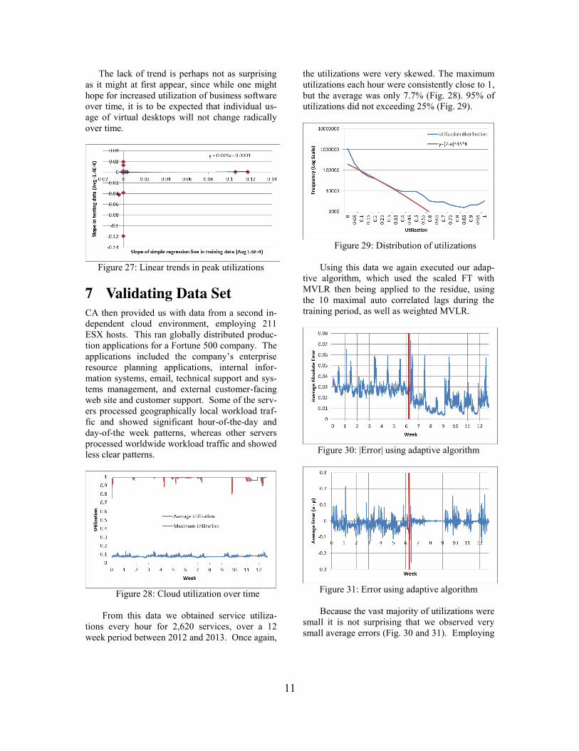
The lack of trend is perhaps not as surprising as it might at first appear, since while one might hope for increased utilization of business software over time, it is to be expected that individual us-age of virtual desktops will not change radically over time.

Figure 27: Linear trends in peak utilizations

7 Validating Data Set CA then provided us with data from a second in-dependent cloud environment, employing 211 ESX hosts. This ran globally distributed produc-tion applications for a Fortune 500 company. The applications   included   the   company’s   enterprise  resource planning applications, internal infor-mation systems, email, technical support and sys-tems management, and external customer-facing web site and customer support. Some of the serv-ers processed geographically local workload traf-fic and showed significant hour-of-the-day and day-of-the week patterns, whereas other servers processed worldwide workload traffic and showed less clear patterns.

Figure 28: Cloud utilization over time

From this data we obtained service utiliza-tions every hour for 2,620 services, over a 12 week period between 2012 and 2013. Once again,

the utilizations were very skewed. The maximum utilizations each hour were consistently close to 1, but the average was only 7.7% (Fig. 28). 95% of utilizations did not exceeding 25% (Fig. 29).

Figure 29: Distribution of utilizations

Using this data we again executed our adap-tive algorithm, which used the scaled FT with MVLR then being applied to the residue, using the 10 maximal auto correlated lags during the training period, as well as weighted MVLR.

Figure 30: |Error| using adaptive algorithm

Figure 31: Error using adaptive algorithm

Because the vast majority of utilizations were small it is not surprising that we observed very small average errors (Fig. 30 and 31). Employing

12

MVLR on the scaled FT residue (as before) re-duced the average absolute error during the train-ing period, and corrected the bias introduced into the average error by scaling the FT.

The adaptive algorithm again performed better

than either of the prediction algorithms it was based on (Fig. 32 and 33).

Figure 32: Accuracy of algorithm for |u-p|≤0.025

Figure 33: Accuracy of algorithm for |u-p|≤0.075

For small utilizations, the adaptive algorithm

was exploiting the scaled FT+MVLR. But for peak utilizations, the adaptive algorithm was clearly exploiting weighted regression (Table 3).

FT+MVLR (1+u)^14 Both Good 0.463698 0.285634 0.749332 Bad 0.121118 0.12955 0.250668 Used 0.584816 0.415184 1.0

Table 3: The adaptive algorithms metrics

FT+MVLR (1+u)^20 Both Good 0.524988 0.250245 0.775233 Bad 0.107134 0.117633 0.224767 Used 0.632122 0.367878 1.0

Table 4: The metrics for (1+u)^20

When a weighting of (1+u)^20 was used the overall results were very similar, but the metrics were slightly better (Table 4).

As a further validation of our approach we

then used the function (2-f(u)/max(f))^14 within the weighted MVLR. The results are similar to Figure 32, but show improvement in some utilizations at the expense of others (Fig. 34 and Table 5).

Figure 34: Using weights (2-f(u)/f(max))^14

FT+MVLR Weighted Both Good 0.537169 0.211399 0.748569 Bad 0.114686 0.136745 0.251431 Used 0.651855 0.348145 1.0

Table 5: (2-f(u)/max(f))^14 metrics

8 Threats to validity

This research was predicated on two sources of data that described performance of a very large number of physical and virtual services, running in two cloud environments, during a comparative-ly short six month interval. While there was con-siderable variability in the behaviour of these services, as a collective they appeared for the most part to be idle. This may not be typical within all cloud computing environments.

The appearance that these machines were not

heavily utilized might be flawed. Average hourly utilization, can potentially be low, even if there are bursts of intense activity within that hour. Performance information was sometimes unavail-able, as consequence of either the machines being deactivated, or the monitoring software being disabled. It is not known how such disruptions impacted upon the averages provided us.

13

We made a best effort to accommodate miss-ing data, but assumptions as to what missing val-ues might have been, necessarily compromise predictive algorithms. Our decision to truncate utilizations greater than 1.0 to 1.0, and to set an upper bound on predicted utilizations at 1.0, helped ensure that prediction appeared closer to high actual utilizations than might otherwise have been the case.

In the second data set, we considered estimat-

ing the maximal CPU usage that each service would require, by discovering its maximum utili-zation within the training period, so as to normal-ize the range of utilizations across the various services.

This highlights a subtle difficulty with predict-

ing service utilizations. We have been assuming that a service running at close to its maximum allowed CPU utilization is using sufficient CPU resources to be of concern to cloud placement algorithms, while those running at a small fraction of their maximum allowed CPU utilization, are of perhaps less concern. These assumptions only hold if each service is itself assigned sensible and meaningful restrictions on how much CPU pro-cessing power it can legitimately exploit.

While multivariate linear regression can be

expected to respond appropriately to changing trends, our presumption (predicated on studying the data) was that no trend would be present with-in long-term seasonality. If trends were present within the observed seasonality, it would be nec-essary to attempt to scale the seasonality using something more complex than a simple linear equation.

A final caveat is in order. No matter how

good a predictive algorithm is, or how much confidence can be place in it, it is inevitable that it will sometimes give misleading results. And it is possible that a few misleading results will more than undermine the benefits of relying on such algorithms.

9 Conclusions System utilization can peak both as a consequence of regular seasonality considerations, and as a consequence of a variety of anomalies, that are inherently hard to anticipate. It is not clear that

the optimal way of predicting such peak system activity is through standard approaches such as multivariate linear regression, since prediction is predicated on the totality of the data observed, and tends to produced smoothed results rather than results that emphasize the likelihood of sys-tem usage approaching or exceeding capacity.

We have presented a number of modifications

to standard multivariate linear regression (MVLR), which individually and collectively improve the ability of MVLR to predict peak utilizations with reasonably small average absolute error.

We found that windowing and scaling MVLR

results to match the observed variance in the input, produced improvement. Applying MVLR to powers of the input data, and employing weighted MVLR, proved to be good techniques for fitting predictions to large but infrequently observed utilizations, but resulted in worse fits against low utilizations.

We explored seasonality using Fourier trans-

forms and have suggested how scaling can im-prove the predictive capability of this analysis. We then suggested how MVLR can be applied to the residue that remains when seasonality is sub-tracted from the input data, to further improve predictive capability.

Within the data provided us, there was often

crossover regions where particular algorithms could be seen to transition from providing better performance than the competition, to worse per-formance. Armed with the ability to determine which side of the crossover a future system pre-diction was likely to be, we developed a hybrid algorithm, which adaptively decided to employ differing predictive strategies, predicated on the recently observed accuracy of these strategies.

This adaptive algorithm leveraged Fourier

analysis, auto correlation, MVLR, scaling and weighted MVLR, to improve our predictive capa-bilities further.

Significantly, the adaptive algorithm achieved

a relatively flat distribution of average absolute errors, across all observed utilizations, even though great asymmetry existed between the fre-quencies of high and low utilizations.

14

This adaptive algorithm provided the best pre-diction of service utilizations, when compared to all other approaches, across the spectrum of ob-served utilizations, on two separate cloud envi-ronments.

With the data provided us, we were able to ob-

tain good short-term (future hour) predictions of system utilization and to achieve good prediction of longer-term trends (measured in months). Both are needed. We believe that the methods em-ployed here have wide applicability, not only to utilizations within clouds, but also to other time series.

In practice cloud environments track statistics

about many variables, such as disk I/O, network I/O, memory usage, etc. Extending the number and type of predictive algorithms used by our adaptive algorithm; improving the mechanisms for obtaining good predictions within our adaptive algorithm; and increasing the number of input time series exploited by an adaptive algorithm, remain opportunities for further research.

We hope that the ideas presented here will be

implemented within commercial cloud placement and scheduling managers, thus permitting greater utilization of cloud resources, at reduced costs, while also permitting better planning and provi-sioning of cloud resources.

Acknowledgements

This research is supported by grants from CA Canada Inc., and NSERC. It would not have been possible without the interest, assistance and en-couragement of CA. Allan Clarke, Laurence Clay and Victor Banda of CA provided valuable input to this paper.

About the Authors

Ian Davis is a Research Associate, Hadi Hemmati is a Post-Doc, Michael Godfrey is an Associate Professor, and Richard Holt is a Professor in the Software Engineering department of the School of Computer Science at the University of Waterloo. Douglas Neuse is a Senior Principal Software Architect and Serge Mankovskii is a Research Staff Member with CA Technologies.

References

[1] A. Amin, A. Colman, L. Grunske: An Approach to Forecasting QoS Attributes of Web Services Based on ARIMA and GARCH Models. ICWS 2012: 74-81

[2] A. Amin, L. Grunske, A. Colman, An auto-mated approach to forecasting QoS attributes based on linear and non-linear time series modeling. International Conference on Au-tomated Software Engineering, 2012.

[3] M. Andreolini and S. Casolari, Load prediction models in web based systems. Proceedings of the 1st international conference on Performance evaluation methodolgies  and  tools” ACM: Pisa, Italy. 2006

[4] M. Arlitt and T. Jin, Workload characteriza-tion of the 1998 World Cup Web site. Tech-nical Report HPL-1999-35R1, HP Labs, 1999.

[5] J.S. Armstrong. Evaluating forecasting methods. Principles of forecasting. A Handbook for Researchers and Practitioners. Kluwer Academic Publishers. 2001

[6] CA Technologies. http://www.ca.com [7] P.K. Chan, M.V. Mahoney. Modeling

multiple time series for anomaly detection. IEEE 5th Int. Conf. on Data Mining. 2005

[8] I.J. Davis, H. Hemmati, et al. Storm prediction in a cloud. 5th Int. Workshop on Principles of Engineering Service-Oriented Systems PESOS, San Francisco. 2013.

[9] P. A.  Dinda  and  D.  R.  O’Hallaron.  Host load prediction using linear models. Journal Cluster Computing. Vol. 3. Issue 4. 2000

[10] N.R. Draper, H. Smith. Applied regression analysis, Third Edition. Wiley Series in Probability and Statistics. 1998

[11] M. Duan. Time series predictability. PhD Thesis. Marquette. 2002

[12] W. Fair. Jr. An algorithm for weighted linear regression. Code Project. 2008

[13] M. Frigo and S. Johnson. The Fastest Fourier Transform in the West. MIT-LCS-TR-728. Massachusetts Institute of Technology. 1997

[14] A. S. Ganapathi. Predicting and optimising system utilization and performance via statistical machine learning. PhD Thesis. University of California. Berkeley. 2009

15

[15] D. Gmach, J. Rolia, L. Cherkasova, A Kemper. Workload analysis and demand prediction of enterprise data centre applications. Proc. IEEE 10th Int. Symposium on Workload Characterization. 2007

[16] J. G. D. Gooijer and R. J. Hyndman, 25 Years of time series forecasting. International Journal of Forecasting, vol. 22, issue 3, 2006, pp. 442–473

[17] Y. Huhtala. J. Karkkainen. and H. Toivonen. Mining for similarities in aligned time series using wavelets. Proc. SPIE Vol 3695. Data Mining and Knowledge Discovery: Theory, Tools and Technology. 1999

[18] E. Hurwitz, T. Marwala. Common mistakes when applying computational intelligence and machine learning to stock market model-ling. 22 August 2012. http://arxiv.org/abs/1208.4429v1

[19] M. Istin., A. Visan, F. Pop, and V. Cristea. Decomposition based algorithm for state pre-diction in large scale distributed systems. 9th International Symposium on Parallel and Distributed Computing. Istanbul, Turkey. 2010

[20] S. Kavulya, J. Tan, R. Gandhi, P. Narasim-han, An analysis of traces from a production mapreduce cluster. Int. Symposium on Clus-ter, Cloud, and Grid Computing, 2010.

[21] A. Khan, X. Yan, S. Tao, N. Anerousis. Workload characterization and prediction in the cloud. A multiple time series approach. Network Operations and Management Sym-posium (NOMS). April 2012

[22] M.S. Magnusson. Discovering hidden time patterns in behavior: T-patterns and their detection. Behaviour Research Methods, Instruments and Computers. Feb 2000, 32(1).

[23] X. Meng, V. Pappas, L. Zhang, Improving the Scalability of Data Center Networks with Traffic-aware Virtual Machine Placement. In-ternational Conference on Computer Com-munications, 2010.

[24] R. Nathuji. A. Kansal, and A. Ghaffarkhah. Q-Clouds: Managing performance interference effects for QoS-aware clouds. Proc. 5th European Conf. on Computer Systems. EuroSys. 2010

[25] D. Neuse, S. Oberlin, P. Peterson, S. Williamson. Workload forecasting research – business problem and solution value. (Internal CA power point presentation). May 12, 2012

[26] S. Nikolov. Trend or no trend: A novel nonparametric method of classifying time series. PhD Thesis. MIT. 2011

[27] R.J. Povinelli. Time series data mining: Identifying temporal patterns for characterization and prediction of time series events. PhD Thesis. Milwaukee, Wisconsin. December 1999

[28] J. Srinivasan and N. Swaminathan. Predicting behavior patterns using adaptive workload models. Proc. 7th International Symposium on Modeling, Analysis and Simulation of Computer and Telecommunication Systems. 1999

[29] M. Stokely, A. Mehrabian, C. Albrecht, F. Labelle, A. Merchant. Projecting disk usage based on historical trends in a cloud environment. Proc. 3rd Int. Workshop on Scientific Cloud Computing. 2012

[30] J. Tan, P. Dube, X. Meng, L. Zhang. Exploit-ing, Resource Usage Patterns for Better Utili-zation Prediction. International Conference on Distributed Computing Systems Work-shops, 2011.

[31] A. Williams, M. Arlitt, C. Williamson, K. Barker, Web Content Delivery, chapter Web Workload Characterization: Ten Years Later. Springer, 2005

[32] D.W. Yoas. and G. Simco. Resource utilization prediction: A proposal for information technology research. ACM Joint Conference on IT Education and Research in IT. 2012

[33] T. Zheng, M. Litoiu, M. Woodside. Integrated Estimation and Tracking of Performance Model Parameters with Autoregressive Trends. ICPE’11. March 14–16, 2011