regression discontinuity designs with multiple assignment ... · pdf fileregression...

Regression Discontinuity Designs with Multiple

Assignment Variables ∗

Yizhuang Alden Cheng

April 11, 2016

Abstract

In this paper, I extend current research on regression discontinuity(RD) designs with multiple assignment variables. I discuss the assump-tions underlying the validity of such RD designs, and introduce graphicalmethods that check for violations of these assumptions. Instead of esti-mating a scalar treatment effect as in RD designs with a single assignmentvariable, I propose estimating treatment functions that are defined on theboundaries that separate different treatment groups in the assignmentvariable space. I generalize a local linear regression method currentlyused for estimation of said treatment functions, and separately developa novel estimation method using thin plate regression splines. The per-formances of these estimation methods are assessed through an extensivesimulation study based closely on real data.

1 Background

The regression discontinuity (RD) design, first introduced by Thistlewaite andCampbell (1960), has enjoyed a revival in popularity over the past two decades.As Lee and Lemieux (2010) document, the RD method has been used for a widerange of policy evaluations, in areas such as education, labor market programs,health and crime. In RD designs, treatment status is determined by whether anassignment variable passes a threshold. Under the assumption that the locationof observations near this cutoff is as-good-as-random, the treatment effect isidentified as the difference in mean outcomes for observations just above andbelow the cutoff.

In practice however, there are many instances where treatment is determinedby more than one assignment variable, such as when numerous criteria deter-mine eligibility for a benefit, or when students need to achieve a minimum scorefor each component of an exam in order to move onto the next grade level.Multiple-assignment variable RD (MRD) designs estimate treatment effects for

∗I would like to thank my thesis adviser, Professor David Card, for all of his support andinsights. All errors in this paper are mine alone.

1

such instances by considering observations near the boundaries separating differ-ent treatment groups in the multidimensional assignment variable space. MRDsfall under two general categories – cases with dichotomous treatments (the twotreatment conditions being either treatment or control), and those with multipletreatments (i.e., more than two mutually exclusive treatment conditions). Forthe latter category, treatment effects are only defined for pairwise comparisonsof treatment conditions, so there is no natural “control” group. To avoid confu-sion, I adopt the following taxonomy for different categories of RDs throughoutthe rest of this paper:

Conventional RD: One assignment variable/Dichotomous treatment;

MDRD: Multiple assignment variables/Dichotomous treatment;

MMRD: Multiple assignment variables/Multiple mutually exclu-sive treatment conditions.

The next example illustrates the difference between MDRD and MMRD.Consider first an exam that has a math and reading component, both of

which students must pass in order to move onto the next grade level. Thereare two assignment variables (math and reading test scores) and dichotomoustreatment (whether or not the student moves onto the next grade), making thisa MDRD. Next, consider a slightly modified scenario, in that students who onlyfail one of the components are merely required to attend remedial classes. Thisis now a MMRD with two assignment variables and multiple mutually exclusivetreatment conditions (grade retention, remedial classes, or moving onto the nextgrade).

While various papers have used MRD for analysis, the estimands of inter-est and estimation methods used are extremely varied. This is because, un-like for conventional RD, there is scant literature on methods for MRD, thefollowing papers being rare exceptions. Wong, Steiner and Cook (2013) com-pare four different estimation methods for MDRD. Papay, Willett and Murnane(2011a) define MMRD, and propose a specific method of estimation. Reardonand Robinson (2012) briefly discuss both types of MRD.

This paper extends the nascent literature on both categories of MRD in sev-eral ways. First, I justify the estimation of treatment effect functions ratherthan scalar treatment effects, and introduce key assumptions underlying thevalidity of MRD. Then, I develop graphical analysis methods specifically tai-lored for MRD. Such graphical presentations can enhance transparency of theresearch design and check for violations of the identifying assumptions. Next, Imodify an existing estimation method to address its limitations, and separatelydevelop a novel estimation method for MRD using thin plate regression splines.In an extensive simulation study, estimation via thin plate regression splinesoutperforms other conventional estimation methods.

The rest of this paper is organized as follows. Section 2 briefly reviews con-ventional RD, defines both types of MRD formally, and outlines the assumptionsthat underpin these RD designs. Section 3 discusses graphical analysis meth-ods for MRD. Section 4 describes a generalization of an existing estimation

2

approach, and proposes a novel estimation method which uses thin plate re-gression splines. Section 5 covers a simulation study modeled closely on datafrom Kane (2003). Section 6 discusses additional issues such as fuzzy MRD andsection 7 concludes.

2 Regression Discontinuity Designs

This section covers the basics of conventional RD and MRD, introducing nota-tion that will be used throughout this paper. Key assumptions underlying thevalidity of these designs, as well as estimands of interest are stated.

2.1 Conventional RD

I begin this section by briefly reviewing the conventional RD design, since itmotivates most concepts in MRD. Given a sample of size N , I denote the treat-ment indicator for observation i by Wi. A sharp RD design is assumed, so Wi

is completely determined by the value of a one-dimensional assignment variableXi, which I assume to be continuous for now. To simplify notation, I assumewithout loss of generality that Xi has been centered about its cutoff, and thatthe assignment rule is:

Wi ≡ I[Xi >= 0].

I write the potential outcomes as Yi(0) and Yi(1), where the observed out-comes are Yi = Yi(0) for observations with Xi < 0, and Yi = Yi(1) for observa-tions with Xi ≥ 0. The key identification assumption for the conventional RDdesign is that the conditional expectation functions of potential outcomes arecontinuous at the cutoff for the assignment variable Xi:

limx→0+

E[Yi(0)|Xi = x] = limx→0−

E[Yi(0)|Xi = x], and

limx→0+

E[Yi(1)|Xi = x] = limx→0−

E[Yi(1)|Xi = x].

A stronger assumption – that the conditional expectation functions are con-tinuous over their domains of definition – is often used in practice, since itis hard to imagine the weaker assumption being met but with discontinuitiesoccurring at non-cutoff points in a well-formulated problem.

Under this setup, the estimand of interest is

(1) τRD = limx→0+

E[Yi|Xi = x]− limx→0−

E[Yi|Xi = x].

2.2 MDRD

This subsection introduces RD designs with multiple assignment variables anddichotomous treatment, which I abbreviate as MDRD throughout this paper.For most of the paper, I focus on the case with d = 2 assignment variables for

3

notational simplicity. However, most of the discussion can easily be generalizedto instances where d > 2. Again, I assume that the assignment variables havebeen centered about their cutoffs and denote the assignment variables for ob-servation i by X1i and X2i. Occasionally, I use the notation Xi to denote thevector of assignment variables in a MRD design.

Retaining the notation for potential outcomes, I assume without loss ofgenerality that the assignment rule is of the “AND” type (i.e. in order toqualify for treatment, the cutoffs for both assignment variables must be met)1:

Wi ≡ D1i ×D2i = I[X1i ≥ 0 and X2i ≥ 0], where

D1i ≡ I[X1i ≥ 0] and D2i ≡ I[X2i ≥ 0].

Here, in contrast to the conventional case where there is a single scalarcutoff, there are two thresholds, one for each assignment variable. Moreover, theassignment variable space in MRD is of dimension d = 2, so that the boundariesseparating different treatment groups have dimension d− 1 = 1. The treatmentfrontiers are defined as:

F1 ≡ {(x1, x2)|x1 = 0 and x2 ≥ 0}, and

F2 ≡ {(x1, x2)|x1 ≥ 0 and x2 = 0}.

In order to estimate treatment effects using these frontiers, certain continuityassumptions for the conditional expectation functions of the potential outcomesare needed. The assumptions for Y (1) are that

limx1→0+

E[Yi(1)|X1i = x1, X2i = x2] =

limx1→0−

E[Yi(1)|X1i = x1, X2i = x2] for x2 ≥ 0,

limx2→0+

E[Yi(1)|X1i = x1, X2i = x2] =

limx2→0−

E[Yi(1)|X1i = x1, X2i = x2] for x1 ≥ 0,

and similarly for Y (0), as Wong et al. (2013) note. Once again, it may be rea-sonable to assume that these conditional expectation functions are continuous

1As an example of why it suffices to consider “AND” assignment rule, consider the following“OR” assignment rule:

Wi = I[X1i > 0 or X2i > 0].

In this case, I can simply redefine the treatment indicator and assignment variables by

Wi ≡ 1−Wi, X1i ≡ −X1i, X2i ≡ −X2i.

This yields

Wi = I[X1i ≤ 0 and X2i ≤ 0] = I[X1i ≥ 0 and X2i ≥ 0],

which is in the form of an “AND” assignment rule.

4

over their domains of definitions, although this is a stronger assumption thannecessary.

Unlike in conventional RD, there is some ambiguity over the estimand ofinterest in MRD. Let Gi = Yi(1)−Yi(0) be the difference in potential outcomesfor observation i, g(x1, x2) be the difference in expected potential outcomes as afunction of the assignment variables, and f(x1, x2) be the joint density functionfor (X1, X2).

Wong et al. (2013) consider the two frontier-specific treatment effects andthe overall treatment effect to be the estimands of interest, and introduce a“frontier approach” that estimates these three quantities. Using this paper’snotation, the treatment effects specific to F1 and F2 are

(2) τWong1 ≡ E[Gi|(X1i, X2i) ∈ F1] =

∫x2≥0 g(0, x2)f(0, x2)dx2∫

x2≥0 f(0, x2)dx2, and

(3) τWong2 ≡ E[Gi|(X1i, X2i) ∈ F2] =

∫x1≥0 g(x1, 0)f(x1, 0)dx1∫

x1≥0 f(x1, 0)dx1

respectively. The overall treatment effect

(4) τWongMDRD ≡ E[Gi|((X1i, X2i) ∈ F1 ∪ F2)] = w1τ

Wong1 + w2τ

Wong2 ,

is a weighted average of the frontier-specific treatment effects, with the weightsrespectively reflecting the probability of an observation being in each of thefrontiers (conditional on being on one of the frontiers):

(5) w1 ≡∫x2≥0 f(0, x2)dx2∫

x1≥0 f(x1, 0)dx1 +∫x2≥0 f(0, x2)dx2

, and

(6) w2 ≡∫x1≥0 f(x1, 0)dx1∫

x1≥0 f(x1, 0)dx1 +∫x2≥0 f(0, x2)dx2

.

However, there are several aspects to this approach that are undesirable.First, as Wong et al. (2013) note, the estimated overall treatment effect

is not invariant to rescaling of the assignment variables. This problem is lessserious when the assignment variables are measured in comparable scales, forinstance when they represent scores on different components of a test, as inJacob and Lefgren (2004) and Matsudaira (2008). However, there are also caseswhere the units of measurement for assignment variables are not aligned, such aswith parental income and high school GPA, which are the assignment variablesused in Kane (2003). There does not seem to be a natural scaling of GPA andincome that would make the units of measurement “comparable”, and the factthat the overall treatment effect estimate depends on such an arbitrary scalingdecision diminishes the credibility of this estimate.

Second, potentially interesting heterogeneities in the treatment effect may belost in summarizing the effects as scalar quantities. For example, Kane (2003)

5

investigates how financial aid affects the college going decision, where the as-signment variables determining aid eligibility are high school GPA and parentalincome. The treatment effect at the GPA threshold τWong

GPA is a weighted averageover students with different family incomes (below the income threshold). Yet,one may suspect that at the GPA frontier, the treatment effect would be greaterfor students with lower family income, since financial constraints are presumablya greater barrier to college going for these students. It would not be possibleto test the validity of this conjecture using the scalar treatment effect estimatesproposed by Wong et al. (2013).

Finally, Wong et al. (2013) admit that their approach requires the strongassumption that the response surface g(x1, x2) is correctly specified. Moreover,estimation of the joint density f(x1, x2) and numerical integration requires largeamounts of data and is computationally expensive.

This paper proposes estimating treatment functions instead of scalar treat-ment effects. Specifically, I estimate the functions

(7) τ1(x2) ≡ E[Yi(1)− Yi(0)|X1i = 0, X2i = x2],

(8) τ2(x1) ≡ E[Yi(1)− Yi(0)|X1i = x1, X2i = 0]

for x2 ≥ 0 and x1 ≥ 0 respectively. Assuming that the expectations of potentialoutcomes conditional on the assignment variables are continuous, it follows thatτ1(x2) and τ2(x1) are continuous functions and that their values coincide at theintersection of the treatment frontiers, i.e. τ1(0) = τ2(0).

This approach is both simpler and circumvents most shortcomings of the“frontier approach” proposed by Wong et al. (2013). In particular, estimationof treatment effect functions does not require density estimation or numericalintegration, and these functions capture variations in treatment effects overdifferent subpopulations near the treatment frontiers.

2.3 MMRD

With more than one assignment variable, it is not uncommon for there to bemultiple mutually exclusive treatments, as exemplified by the numerous exam-ples given by Papay et al. (2011a). This necessitates additional notation, andthe assignment rule from MDRD needs to be modified for MMRD2.

2I assume here for simplicity of exposition, that there are four treatment conditions, withboth assignment variables centered at their cutoffs. Papay et al. (2011a) note that in generalwith d assignment variables, there are 2d different treatments. In fact, there may be moreor less than 2d different treatments. An example with two assignment variables and threetreatments is given in the introduction – the treatments being (i) forced to stay back a gradeif both tests are failed; (ii) summer remedial classes if only one test is failed; (iii) moving ontothe next grade if both tests are passed. Cases with two assignment variables and more thanfour possible treatments are also imaginable when there are multiple cutoffs.

6

X1

X2

Wi = 1

Wi = 0

X1

X2

W1i = 1W2i = 1

W3i = 1 W4i = 1

Figure 1: An illustration of the difference between MDRD (left panel) andMMRD (right panel)

To simplify notation, I denote the four quadrants of the assignment variablespace by

R1 ≡ {(x1, x2)|x1 ≥ 0, x2 ≥ 0},R2 ≡ {(x1, x2)|x1 < 0, x2 ≥ 0},R3 ≡ {(x1, x2)|x1 < 0, x2 < 0},R4 ≡ {(x1, x2)|x1 ≥ 0, x2 < 0}.

Indicators for the four treatments can thus written as

Treatment 1: W1i ≡ D1i ×D2i = I[Xi ∈ R1],

Treatment 2: W2i ≡ (1−D1i)×D2i = I[Xi ∈ R2],

Treatment 3: W3i ≡ (1−D1i)× (1−D2i) = I[Xi ∈ R3],

Treatment 4: W4i ≡ D1i × (1−D2i) = I[Xi ∈ R4].

Similarly, there are four different treatment frontiers which coincide withthe non-negative and negative x1- and x2-axes. A treatment effect function isestimated along each of these frontiers. The frontier separating treatments 1and 2 is

F12 ≡ {(x1, x2) x1 = 0 and x2 ≥ 0}

7

and the treatment effect function (moving from treatment 1 to 2) is denoted

(9) τ12(x2) ≡ E[Yi(2)− Yi(1)|X1i = 0 and X2i = x2].

The other frontiers F23, F34 and F14, and treatment effect functions τ23(x1),τ34(x2) and τ14(x1) are defined analogously. These treatment effect functionsrepresent the effect of moving from treatment condition 3 to 2, 3 to 4, and 4 to1 respectively3.

Validity of the MMRD design once again relies on the conditional expecta-tion of the potential outcomes obeying certain continuity conditions along thetreatment frontiers. For instance, denoting the four potential outcomes by Y (1),Y (2), Y (3) and Y (4), estimation of τ12(x2) requires

limx1→0+

E[Yi(1)|X1i = x1, X2i = x2] = limx1→0−

E[Yi(1)|X1i = x1, X2i = x2],

limx1→0+

E[Yi(2)|X1i = x1, X2i = x2] = limx1→0−

E[Yi(2)|X1i = x1, X2i = x2],

for x2 ≥ 0. Analogous continuity assumptions are necessary for the estimationof τ23(x1), τ34(x2) and τ14(x1).

As before, it is not unreasonable to ask that the conditional expectation func-tions for the four potential outcomes be continuous over the entire assignmentvariable space.

However, it is worth mentioning that in general for (i1, j1) 6= (i2, j2), theequality τi1j1(0) = τi2j2(0) may not hold (unlike in MDRD)4, which is due tothere being more than two treatment functions under consideration. To explainwhy this is reasonable, consider an example with math and reading test scoresas assignment variables determining four possible treatments – grade retention,math remedial classes over summer, reading remedial classes over summer, andmoving onto the next grade level. It is clear in this case that there is no reason toexpect the treatment effect which compares grade retention and summer mathclass, to be similar to the treatment effects comparing reading or math class tono remedial, even for pairs of test scores that are relatively close in Euclideandistance.

Another noteworthy issue is the fact that although there are(42

)= 6 dif-

ferent pairs of treatment conditions that one may wish to compare, this paperonly focuses on comparing treatments that are separated by a one-dimensionalboundary in the assignment variable space (i.e. the non-negative or negative x1or x2-axis). I omit comparisons of treatments 1 and 3, as well as 2 and 4, whichhave treatment boundaries that contain only a single point – the origin. Inpractice, this often implies that there is an insufficient number of observations(near the boundary) to estimate these treatment effects precisely.

3Strictly speaking, there are two treatment effects that can be estimated along each frontier,corresponding to a movement from one treatment to the other, and the movement in theopposite direction. Since these two treatment effect estimates will simply be of opposite signs,I only choose one treatment effect function to consider for each frontier.

4For a simple illustration of this, consider the case where the potential outcomes are deter-ministic, so that Yi(k) = k for k ∈ {1, 2, 3, 4}. Under this setup, τ12(0) = −1 6= −3 = τ14(0).

8

3 Graphical Analysis

Graphical analysis is critical in establishing the credibility of conventional RDdesigns. Typically, one plots the outcome variable as a function of the assign-ment variable, then examines the graph for the presence of a discontinuity at thecutoff value of the assignment variable, which may be taken as visual evidenceof a nonzero treatment effect. The same is sometimes done for the treatmentindicator variable. Diagnostic plots are also useful for checking whether the iden-tifying assumptions of the RD design are being violated. A common diagnosticplot graphs predetermined characteristics as functions of the assignment vari-able. Another frequently used diagnostic plot is a histogram of the assignmentvariable. Graphical analysis methods for conventional RD are well-documentedin survey papers such as Imbens and Lemieux (2008) and Lee and Lemieux(2010).

While relatively easy to implement for conventional RD, greater dimension-ality in the MRD setting presents additional challenges. Most relevant amongthese is the fact that the visual impact of plots in more than two dimensions isgreatly diminished. Perhaps due to this difficulty, there has been no discussionon graphical analysis in the current MRD literature that I am aware of. In thissection, I review the common plots used in conventional RD and discusses howthey may be generalized appropriately for the MRD setting.

3.1 Discontinuity in Outcomes

The most common graph used in conventional RD plots the outcome variable asa function of the assignment variable. This graph is designed to provide visualevidence of a discontinuity in outcomes at the cutoff, which would suggest a non-zero treatment effect. The procedure for conventional RD typically involvespartitioning the assignment variable space into disjoint bins (or intervals) ofconstant width, computing the average outcomes within each bin, and plottingthese average outcomes against midpoints of the bins. Care must be takenin defining the intervals so that the cutoff does not lie in the interior of anyinterval; otherwise, this would result in a point that aggregates outcomes forobservations from both treatment conditions, making it hard to interpret. Apolynomial regression line is often fitted to points on each side of the cutoff toimprove the visual impact of the plot.

More formally, given a bandwidth h, one first constructs K intervals

[b0, b1), [b1, b2),..., [bK−1, bK),

s.t. 0 ∈ {b1, ..., bK−1},bk − bk−1 = h for all k ∈ {1, ...,K},min{xi} ∈ [b0, b1) and max{xi} ∈ [bK−1, bK).

9

Then, one calculates the average outcomes within each interval,

Yk ≡1

|{i|xi ∈ [bk−1, bk)}|

N∑i=1

Yi · I[xi ∈ [bk−1, bk)] for k ∈ {1, ...,K},

and plots Yk againstbk−1 + bk

2.

Various approaches have been suggested for the choice of h. Lee and Lemieux(2010) propose two – one based on cross-validation, and the other based on visualinspection coupled with an F-test to determine whether h is small enough5. Theguiding principle behind these approaches is to choose h sufficiently small sothat the plot does not “over-smooth” the data, but large enough so that the binestimates are still reasonably precise.

Here, I consider how a similar type of graphical analysis might work in theMRD setting with two assignment variables. I first describe several straight-forward extensions of the procedure for conventional RD, which I argue areeither inappropriate or suboptimal. Then, I introduce the “slicing” and “slidingwindow” approaches, which create plots that are better suited for MRD.

3.1.1 Straightforward Extensions of the Conventional RD Plot thatare Suboptimal

Perhaps the most straightforward extension of the procedure for conventionalRD is to create an analogous graph in three dimensions, using the two assign-ment variables and the outcome variable. Since the assignment variable spaceis two-dimensional, two widths need to be chosen (which I denote by h1 andh2 for X1 and X2 respectively)6. One would then construct P one-dimensionalintervals for X1 and separately, Q intervals for X2, using the same procedure asfor conventional RD. This yields PQ two-dimensional intervals (or bins) whichI denote by

Ip,q ≡ {(x1, x2)|b1,p−1 ≤ x1 < b1,p and b2,q−1 ≤ x2 < b2,q}.

For non-empty intervals, average outcomes within each bin are computed asbefore using the formula

Yp,q ≡1

|{i|(x1i, x2i) ∈ Ip,q|

N∑i=1

Yi · I[(x1i, x2i) ∈ Ip,q],

5Specifically, they consider the regression with K bin dummies (indicating whether anobservation is in a given bin) for bins of width h, as well as an alternative specification with2K bin dummies for bins of width h/2. Since the first model is nested within the second, anF-test can be used to compare the models. A rejection of the null hypothesis would suggestthat the choice of h is too large and that the data is being “over-smoothed”.

6One may be able to get away with choosing a single bin width h for both assignmentvariables if the scales are comparable, e.g. scores for different components of a test. However,I focus on the more general case, since there are many instances where this does not apply,such as when the assignment variables are GPA and income.

10

and plotted over the centers of the bins,

(b1,p−1 + b1,p

2,b2,q−1 + b2,q

2

)in a

three-dimensional graph, possibly with a smoothing surface fitted to each treat-ment region.

The main problem with this graph is that the height (which represents thevalue of the outcome variable) in three dimensional graphs tends to be distorted.In particular, perceptions about the sizes of discontinuities tend to depend onthe “viewpoint” chosen for the plot. It will be especially challenging to choose a“viewpoint” that accurately portrays the discontinuities along all four frontiersin a MMRD. Hence, it may be more appropriate instead to summarize thisinformation using two-dimensional graphs.

For MDRD, an easy way to create a single plot illustrating the disconti-nuity near the boundary makes use of the “centering” approach of Wong etal. (2013)7. The motivating idea is that instead of considering the two assign-ment variables separately, one focuses instead on the distance of an observationfrom the boundary separating the two treatments. Assuming that the scalesof the two centered assignment variables are comparable (otherwise, one maystandardize the variables to have equal variance), one creates a new variable

Zi ≡ inf{d(Xi,X)|X ∈ F1 ∪ F2},

where d denotes a distance function of the user’s choice8. Now, the variable Ziis used as the new assignment variable for graphical purposes, so the approachfor conventional RD can be used.

A similar method may be employed for MMRD, although the two “adjacent”treatments that are being compared need to be specified. This yields four plotsin total (one for each pair of treatments being compared). For instance, tocompare treatments 1 and 2 (which are separated in the assignment variablespace by F12) graphically, one would compute

Zi ≡ inf{d(Xi,X)|X ∈ F12} for i s.t. Xi ∈ R1 ∪R2

and create the conventional RD plot described earlier, using only the subset ofobservations receiving either treatments 1 or 2.

However, this “centering” approach has a major limitation in the dichoto-mous treatment case, in that it does not show frontier-specific treatment effects.By using a single assignment variable Zi instead of the two original assignmentvariables, individuals close to the frontier F1 are treated essentially the same asthose close to the F2. This is especially undesirable when the original assign-ment variables are qualitatively different, so that frontier-specific effects are of

7Although Wong et al. (2013) originally described this as a method for estimation, thegraphical method I describe here is motivated by the same ideas.

8Wong et al. (2013) use the distance function induced by the L∞-norm, although one mayprefer distance functions induced by other norms such as L2 (Euclidean) or L1 depending onthe context.

11

interest (e.g. whether children around the income threshold respond to financialaid differently from children around GPA threshold)9.

A simple method for MDRD that seems to address this shortcoming is toplot two graphs using the procedure for conventional RD. Specifically, for thefirst graph, one takes the graphical approach for conventional RD, treating thefirst assignment variable as if it were the only assignment variable (and likewisefor the second graph using the second assignment variable).

At first glance, this method seems to capture frontier-specific effects (or

more precisely, estimates of τWong1 and τWong

2 ). However, I argue that thisapproach yields misleading graphical estimates. To elaborate, consider the plotwith X1 on the horizontal axis, which should display approximately the averagediscontinuity along F1, i.e. τWong

1 . An outcome Y0+ for a point at (or justabove) the cutoff of zero on this graph should represent an average of the pointsnear F1 that receive the treatment, i.e.

Y0+ ≈ E[Yi|Xi ∈ F1] ≈∫ ∞0

∫ ε

0

y · f(x1, x2)dx1dx2

for some small ε > 0. However, the actual quantity represented by Y0+ is

Y0+ ≈ E[Yi|X1i = 0] ≈∫ ∞−∞

∫ ε

0

y · f(x1, x2)dx1dx2.

The problem is that this method does not take into account the value of theother assignment variable X2, and so the expectation is taken over the entirex2-axis rather than over F1 (the non-negative x2-axis). As a result, observationswith X2i < 0 (which are ineligible for treatment and may be far from F1) areinvolved in the computation of Y0+, which is supposed to represent the averageoutcomes for individuals just qualifying for treatment (along the F1 frontier).Hence, graphs produced by this approach are essentially uninterpretable.

This problem can be fixed with a simple modification – when plotting thegraph using X1 as the assignment variable, instead of using all the data, oneonly uses observations with X2 ≥ 0 (and vice versa when constructing the graphfor X2). This approach is similar in spirit to the “univariate” estimation methoddiscussed in Wong et al. (2013). For MMRD, there is no difference betweenthis method and the “centering” approach described earlier.

Nonetheless, it is possible to do better, since the estimands of interest inthis paper are the treatment functions τ1(x2) and τ2(x1), rather than the scalar

treatment effects τWong1 and τWong

2 . The remainder of this subsection presentstwo graphical methods that are more appropriate for displaying non-constanttreatment effects – the “slicing” and “sliding window” plots.

9This drawback is also the main reason this paper does not generally recommend using the“centering” approach for estimation despite the method’s simplicity.

12

3.1.2 “Slicing” and “Sliding Window” Plots

The following method, which this paper calls the “slicing” approach, representsan extension of the “univariate” approach that enables an approximate visualrepresentation of the treatment effect functions10. Here, I focus on the dichoto-mous treatment case and describe the procedure for producing graphs associatedwith τ1(x2). The procedures for τ2(x1), as well as for MMRD are completelyanalogous.

One considers only the subset of observations {(Yi,Xi)|X2i ≥ 0}, and par-titions (or “slices”) this data into disjoint subsets (or “slices”)

Sk ≡ {(Yi,Xi)|X2i ∈ [sk−1, sk)}

for k = 1, ...,K, where 0 = s0 < s1 < ... < sK−1 < sK <∞.Next, for each of these partitions Sk, one treats X1 as the assignment vari-

able in a conventional RD design and creates a two-dimensional plot using asuitable bandwidth. This results in a series of K “slicing” plots, one corre-sponding to each interval of (non-negative) X2. An estimate of the treatmenteffect corresponding to each subset Sk of observations can be obtained usingthe polynomial regressions that are fit to points on each side of the cutoff. Thisyields a crude point estimate of τ1(x2) at a number of values for x2.

The “slicing” method allows one to examine discontinuities in the outcomevariable at the cutoff for one assignment variable (say X1) for different sub-sets of observations (grouped based on values of the other assignment variable,X2). These plots also contain some information on whether the size of thesediscontinuities vary with X2 (i.e. whether the treatment effect function τ1(x2)is constant). However, there are typically only a limited number of these plotsto compare since disjoint subsets of observations are used to create each plot,so the visual evidence on whether τ1(x2) is constant is still rather scant. Hence,I next describe the “sliding window” plot, which essentially summarizes a seriesof “slicing” plots to provide a better visual summary of the treatment effectfunction over its domain of definition.

For concreteness, I once again focus on τ1(x2) in my description of the “slid-ing window” plot (as before, the procedures for creating the plot for τ2(x1),as well as for MMRD are completely analogous). This graph summarizes thediscontinuities occurring at the cutoff for X1 over different intervals of X2. Oneof the main differences in the calculations required to construct this plot versusthe “slicing” plots, is that instead of partitioning the data into disjoint subsetsaccording to values of X2, one creates subsets of data by “sliding” the intervalof X2 under consideration (hence the name of the graph). In particular, theintervals of X2 used for different subsets are no longer disjoint.

There are a few parameters in the “sliding window” plot that the user maychoose to provide the best visual impact – w (the width of intervals for X2),

10In fact, one may think of the “univariate” approach as a special case of the “slicing”approach with K = 1, using the notation introduced below.

13

c (the constant that the interval for X2 is shifted by each time) and h (thebandwidth for X1, controlling the amount of data just above and below thecutoff of X1 to use). The following subsets of {(Yi,Xi)|X2i ≥ 0} are created:

Wk ≡ {(Yi,Xi)|X2i ∈ [(k − 1)c, (k − 1)c+ w)}

for k = 1, ...,K ′, where

K ′ ≡ inf{k ∈ Z|(k − 1)c+ w > max{X2i)}.

For each Wk, let W lk and Wu

k be the subsets of observations in Wk belowand above the cutoff for X1 that are within h of this cutoff respectively. Onethen computes the average values of the outcome variable Y for the subsets W l

k

and Wuk , which I denote by Y lk and Y uk respectively.

The final step in creating the “sliding window” graph is to plot Y lk and Y uk ,against the midpoints of X2 in Wk, which are given by

Xmid2,k =

2(k − 1)c+ w

2.

The vertical distance between Y uk and Y lk is an approximation of τ1(Xmid2,k ).

The procedure just described for τ1(x2) uses a rectangular kernel of widthw for X2 in the calculation of Y lk and Y uk . However, one may reasonably argueagainst this uniform weighting of points within Wk by insisting that observa-tions with values of X2 closer to Xmid

2,k should have a greater impact in the

determination of Y lk and Y uk . The method for constructing “sliding window”plots I described can easily be modified to accommodate other choices of ker-nels with compact support, e.g. triangular or Epanechnikov. In particular, theonly change required is to use weighted averages for Y lk and Y uk . The formulaeare

Y lk =1∑N

i=1 wli,k

N∑i=1

wli,kYi and Y uk =1∑N

i=1 wui,k

N∑i=1

wui,kYi,

where wli,k and wui,k represent the (relative) weights for observation i, which

depends on the sets W lk and Wu

k respectively, as well as on the choice of kernel.In particular, for the three kernels mentioned above, the (relative) weights maybe written as11

Rectangular: wli,k = I[(Yi,Xi) ∈W lk]

wui,k = I[(Yi,Xi) ∈Wuk ];

Triangular: wli,k =

(w

2− |X2 −Xmid

2,k |)· I[(Yi,Xi) ∈W l

k]

wui,k =

(w

2− |X2 −Xmid

2,k |)· I[(Yi,Xi) ∈Wu

k ];

11In the formulae I give for the (relative) weights, I omit the constant of integration sincemy formulae for Y l

k and Y uk include the sum of the weights in their denominators.

14

Epanechnikov: wli,k =

[w

4

2− (X2 −Xmid

2,k )2]· I[(Yi,Xi) ∈W l

k]

wui,k =

[w

4

2− (X2 −Xmid

2,k )2]· I[(Yi,Xi) ∈Wu

k ].

To summarize, in this subsection I described various plots that one may thinkare suitable for displaying the discontinuities in outcome for MRD. I discussedwhy several of these plots are unsuitable, and recommended the “slicing” and“sliding window” plots. The “slicing” plots allow one to separately examine thediscontinuities in outcome for different regions along each treatment frontier.The “sliding window” plot provides additional visual evidence on whether thesediscontinuities are constant along each treatment frontier. Examples of boththese two plots based on a realistic simulated dataset are presented in section 5of this paper.

3.2 Diagnostic Plots

The crucial assumption underpinning validity of conventional RD and MRD de-signs requires that the conditional expectation functions of potential outcomesbe continuous at the cutoffs. Unfortunately, this assumption cannot be testeddirectly, since potential outcomes for any particular treatment are only observedon one side of the threshold (assuming that the RD or MRD is sharp). Nonethe-less, two types of diagnostic plots are often used in conventional RD to test thisassumption indirectly. This subsection briefly reviews the diagnostic plots forconventional RD, and describes how they can be adapted for use in MRD.

3.2.1 Plotting a Predetermined Outcome as a Function of the As-signment Variables

The first type of diagnostic graph often used in conventional RD plots a prede-termined outcome against the assignment variable. For example, if the outcomeis college going and scholarship eligibility is determined by whether one’s SATmath score passes a certain threshold, the diagnostic graph may plot a prede-termined outcome such as the mother’s education level or the student’s highschool GPA against the student’s SAT math score. The motivation is that ifthe values of observations’ assignment variables near the cutoff are genuinelyas-good-as-random, then the baseline characteristics of observations just belowor above the threshold should not differ systematically.

The discussion in the preceding subsection for plotting outcomes againstassignment variables in MRD apply to this diagnostic plot as well. This paperproposes using the “slicing” approach to create these diagnostic plots, withthe predetermined variable (instead of the outcome variable of interest) on thevertical axis.

15

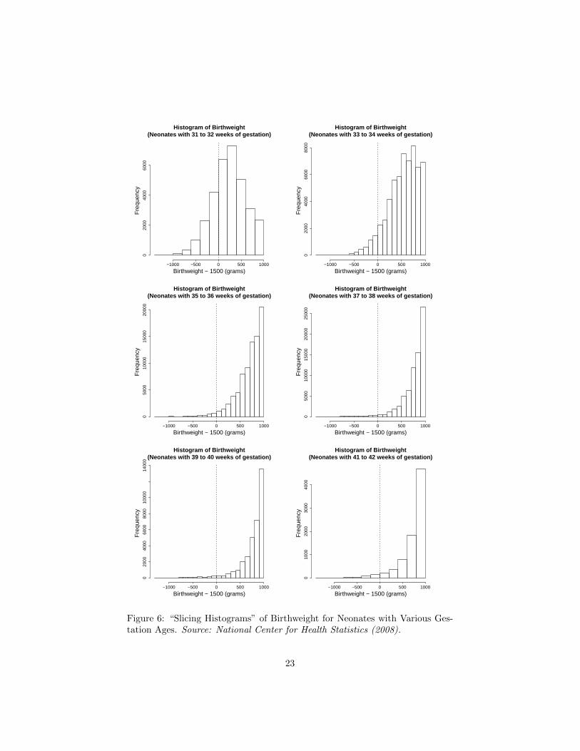
3.2.2 Examining the Density of the Assignment Variables

The second type of diagnostic plot common in conventional RD is a histogramof the assignment variable (where no bin contains the cutoff in its interior).The rectangles immediately to the left and right of the threshold are examinedto get a sense of whether the density of the assignment variable is continuousat the cutoff. An obvious discontinuity would indicate that the locations ofobservations’ assignment variable values near the threshold are not as-good-as-random (or in other words, that the assignment variable is manipulable), whichcalls into question the validity of the RD design.

As an example, suppose that admission to the most prestigious university ina (fictional) country depended on whether the applicant’s admission test scorepassed a certain threshold. The goal is to determine the “value-added” of at-tending this university, using future earnings as the outcome variable. Suppose(rather pessimistically) also that corruption is rampant in this country, and par-ents of rich kids anywhere near the threshold are able to bribe officials gradingthe test into giving their kids a score above the cutoff. In such a case, only kidsin relatively poor families will have test scores that fall just under the cutoff,so that the characteristics of applicants just above and below the cutoff are dif-ferent on average. Hence, the treatment effect estimate may be biased upwardsif rich kids tend to have higher earnings on average independent of ability, dueto better connections and so forth. The validity of the RD design is clearlyviolated, and this will show up in the histogram in the form of the rectangleimmediately to the right of the cutoff being significantly higher than the one toits left.

While the concept of examining the density of assignment variables at thetreatment frontiers in MRD follows straightforwardly from the motivation forthe histogram in conventional RD, implementation is much trickier. A three-dimensional histogram encounters the difficulty of the height (which approxi-mately represents the joint density of the assignment variables) being distorted,a problem mentioned in the previous section for graphs showing discontinuitiesin outcome. This paper suggests two alternatives for displaying the assignmentvariables’ density in MRD with minimal distortion.

The first approach is to display the three-dimensional histogram as a contourplot. The reader can then examine whether the colors of bins on either side ofeach frontier change drastically (which would indicate a likely discontinuity).The main challenge in creating an informative contour plot is the selection ofa suitable color gradient, which is arguably much simpler than the problem ofchoosing an appropriate “viewpoint” for a three-dimensional histogram.

The second approach is similar in spirit to the “slicing” approach describedearlier in this section, with frequency on the vertical axis. The following is amore detailed description of this procedure. Suppose that I intervals are used forX1, and J intervals for X2, so that there is a total of at most IJ bins. For eachof the I intervals for X1, one can create a two-dimensional histogram with the Jintervals for X2 on the horizontal axis, and rectangle heights that represent thenumber of observations with X1 and X2 values within the respective intervals.

16

The same can be done for each unique interval of X2. For a MDRD design, notall of these I+J two-dimensional histograms are relevant, since only histogramsthat contain bins for observations receiving different treatments are relevant12.

Regardless of whether one chooses to use the contour plot or a series of“slicing” histograms to examine the density of the assignment variables, caremust be taken in defining the bins so that no point on the treatment frontiersfalls in the interior of any bin.

3.2.3 Demonstration of Diagnostic Plots using NCHS Dataset

This example demonstrates the recommended diagnostic plots described in theprevious subsection for a MMRD, with neonate birthweights and gestation agesas the assignment variables. Neonates with birthweights or gestation ages belowthe cutoffs of 1500g and 37 weeks are respectively classified as “very low birthweight” and “premature”, and tend to receive extra medical attention as a re-sult. The design for this example is motivated by Almond et al. (2010), whouse a conventional RD design with birthweight as the only assignment variable.Almond et al. do not use gestation age as an assignment variable due to worriesthat it is manipulable. The purpose of this graphical exercise is to determinewhether the inclusion of gestation age as a second assignment variable (in ad-dition to birthweight) violates the assumptions underpinning the validity of theMMRD design13. The dataset used for these plots is the 2008 Cohort Linked

12One may notice that this “slicing” approach is designed only to detect discontinuities inthe density as the frontier is approached from a direction parallel to one of the treatmentfrontiers in the assignment variable space. Hence, it is possible that a discontinuity at somepoint of the frontier may exist that would not be detectable by this method, as illustrated bythe following example.

Suppose that a discontinuity existed at a point (0, x∗2) along the frontier that is the positivex2-axis, where x∗2 > 0. Further assume that

limx1→0+

f(x1, x∗2) = lim

x1→0−f(x1, x

∗2),

but that

limt1→0+

f(−t1, x∗2 + t1) 6= limt2→0+

f(t2, x∗2 + t2),

where f(x1, x2) is the joint density function of the assignment variables. This would representa discontinuity in the joint density function that is not detectable by the “slicing” approach,which can only test whether the limits limx1→0+ f(x1, x∗2) and limx1→0− f(x1, x∗2) are equal.

Nonetheless, while it is easy to construct counterexamples in theory, it is difficult to imaginemanipulation of the assignment variables in practice that would result in such discontinuitiesin practice. For instance, if teachers were manipulating reading and math test scores, theywould have to do so in a way that for each given reading test score, the proportion of studentswith math test scores just above and below the threshold remained roughly the same, andvice versa, switching the roles of reading and math. It is hard to think of why agents mightbe motivated to engage in such contrived manipulation.

13One may realize that although I had been assuming so far that the assignment variableshave continuous support, the measurement of gestation age in weeks is rather coarse, so thatthe support of the gestation age variable “is more discrete than continuous”. Assignmentvariables that have discrete rather than continuous support present issues for treatment effectestimation, as Lee and Card (2008) point out. I revisit this issue in greater detail whendiscussing estimation for MRD in the next section.

17

Birth/Infant Death Data Set, from the National Center for Health Statistics(NCHS).

The first type of diagnostic graph shown here plots a predetermined outcome– mother’s age – against each assignment variable in turn using the “slicing”approach. Linear regression lines are added to the points on each side of thecutoff. Several bandwidths were considered for birthweight and gestation age(25g 50g, 100g and 200g for birthweight and one to five weeks for gestation age).None of these choices resulted in a plot that displayed an obvious discontinuityat the cutoff, which is consistent with a valid MMRD design. The graphs shownin the paper use a bandwidth of 100g for birthweight and one week for gestationage.

The contour plot and the “slicing” histograms, shown next, examine thedensity of the assignment variables near the cutoff. In both plots, signs ofa significant discontinuity at the treatment frontiers are absent. Again, thisresult is to be expected if the MMRD assumptions are not violated.

While no single one of these diagnostic plots can by itself guarantee thevalidity of the MMRD design, taken together, they provide some degree ofassurance that there are no obvious violations of the MMRD assumptions.

4 Estimation

Most estimands in economics seek to capture a global relationship betweencovariates and the outcome variable. By contrast, the estimand of interest inRD designs – being the difference between point estimates of two regressionfunctions at their boundaries – is highly local and far more uncertain. As aresult, issues such as specification error and boundary effects are particularlyrelevant for treatment effect estimation in RD designs.

This has led to a substantial body of literature investigating a variety of para-metric and nonparametric estimation methods for conventional RD. As surveypapers on RD such as Imbens and Lemieux (2008) and Lee and Lemieux (2010)document, some degree of consensus on estimation procedures has developedover time for conventional RD. By contrast, there has been scant research onmethods for MRD, and thus, little by way of consensus on MRD estimation.

This section begins by introducing a few of the most common estimationapproaches for conventional RD, and discusses their advantages and disadvan-tages. Then, I describe an estimation method for MMRD proposed by Papay etal. (2011a). I propose a modification of their method for MDRD estimation andsuggest a generalization of the cross-validation procedure they define. Finally, Idevelop a novel estimation method that addresses some of the shortcomings ofpopular RD estimation approaches, and can be easily implemented for MDRDas well as MMRD.

18

● ●

● ●

●

●

●

●

●

●

−4 −2 0 2 4

2526

2728

2930

Mother's Age as a Function of Gestation Length:Neonates with Birthweight 1100−1299 grams

Gestation Age − 37 (weeks)

Mot

her's

Age

11911 Neonates

●

●

● ●

●

●

● ●

●

●

−4 −2 0 2 4

2526

2728

2930



Mot

her's

Age

15141 Neonates

●

● ●

●

●

●

●

●

●

●

−4 −2 0 2 4

2526

2728

2930



Mot

her's

Age

19536 Neonates

● ●●

●

●

●●

●

●

●

−4 −2 0 2 4

2526

2728

2930



Mot

her's

Age

30168 Neonates

●

●

●

●●

●

●

●

●

●

−4 −2 0 2 4

2526

2728

2930



Mot

her's

Age

43864 Neonates

● ●

●

●

●

●

●

●

● ●

−4 −2 0 2 4

2526

2728

2930



Mot

her's

Age

70743 Neonates

Figure 2: Plots of a predetermined outcome as a function of an assignmentvariable, created using the “slicing” approach. Each of these graphs considersonly neonates with birthweights within a certain interval, and plots mother’sage (the predetermined outcome) as a function of gestation age (the assignmentvariable). A linear regression line is fitted to the points on each side of thecutoff. Source: National Center for Health Statistics (2008).

19

●

●

●

●●

●● ●

● ●

●

●

●

●

●

−400 −200 0 200 400 600 800 1000

2526

2728

2930

Mother's Age as a Function of Birthweight:Neonates with Gestation Age 31−32 Weeks

Birthweight − 1500 (grams)

Mot

her's

Age

45818 Neonates

●

●

●

●

●

●● ● ●

● ● ●

●● ●

−400 −200 0 200 400 600 800 1000

2526

2728

2930



Mot

her's

Age

108142 Neonates

●

●●

●

●

●●

●●

● ●

●

● ● ●

−400 −200 0 200 400 600 800 1000

2526

2728

2930



Mot

her's

Age

304196 Neonates

●

●

●

●

●

●

●

●

●

●

● ● ●● ●

−400 −200 0 200 400 600 800 1000

2526

2728

2930



Mot

her's

Age

1183437 Neonates

●

●

●●

●●

●

●

●

●

●

●●

●

●

−400 −200 0 200 400 600 800 1000

2526

2728

2930



Mot

her's

Age

1942526 Neonates

●

●

●

●

●

●

●

●

● ●

●

●

●

● ●

−400 −200 0 200 400 600 800 1000

2526

2728

2930



Mot

her's

Age

476142 Neonates

Figure 3: Plots of a predetermined outcome as a function of an assignmentvariable, created using the “slicing” approach. Each of these graphs considersonly neonates with gestation ages within a certain interval, and plots mother’sage (the predetermined outcome) as a function of birthweight (the assignmentvariable). A linear regression line is fitted to the points on each side of thecutoff. Source: National Center for Health Statistics (2008).

20

−400 −200 0 200 400

−4

−2

02

4

Contour Plot for 3−Dimensional Histogram


Ges

tatio

n A

ge −

37

(wee

ks)

Figure 4: Contour Plot to Examine the Density of the Assignment Variables.Darker regions represent higher frequencies of observations. Source: NationalCenter for Health Statistics (2008).

21

Histogram of Gestation Age(Neonates with Birthweights of 1200g to 1300g)


Fre

quen

cy

−10 −5 0 5 10

050

010

0015

0020

00



Fre

quen

cy

−10 −5 0 5 10

050

010

0015

0020

0025

00



Fre

quen

cy

−10 −5 0 5 10

050

010

0015

0020

0025

00



Fre

quen

cy

−10 −5 0 5 10

050

010

0015

00



Fre

quen

cy

−10 −5 0 5 10

050

010

0015

00



Fre

quen

cy

−10 −5 0 5 10

050

010

0015

0020

00

Figure 5: “Slicing Histograms” of Gestation Age for Neonates with Birthweightsin Various Intervals. Source: National Center for Health Statistics (2008).

22

Histogram of Birthweight(Neonates with 31 to 32 weeks of gestation)


Fre

quen

cy

−1000 −500 0 500 1000

020

0040

0060

00



Fre

quen

cy

−1000 −500 0 500 1000

020

0040

0060

0080

00



Fre

quen

cy

−1000 −500 0 500 1000

050

0010

000

1500

020

000



Fre

quen

cy

−1000 −500 0 500 1000

050

0010

000

1500

020

000

2500

0



Fre

quen

cy

−1000 −500 0 500 1000

020

0040

0060

0080

0010

000

1400

0



Fre

quen

cy

−1000 −500 0 500 1000

010

0020

0030

0040

00

Figure 6: “Slicing Histograms” of Birthweight for Neonates with Various Ges-tation Ages. Source: National Center for Health Statistics (2008).

23

4.1 Estimation in Conventional RD

A common approach for conventional RD estimation in the past was to fit aglobal polynomial to each side of the cutoff (with the outcome variable as afunction of the assignment variable). This approach has the advantage of beingeasy to implement, but has come under increasing criticism for various reasons,including sensitivity of the treatment estimate to the order of polynomial, andthe boundary effects of higher-order polynomial fits14.

RD estimation via local linear regression has become increasingly widespreadof late, based on properties proved by Fan and Gijbels (1992) and Porter (2003).Yet, while the local linear estimator does not have boundary effects, implemen-tation requires specification of a bandwidth. Generally, choosing an optimalbandwidth involves a variance-bias trade-off. In particular, both the estima-tor’s squared bias and its variance contribute to the expected mean squarederror (MSE) of the treatment effect, which one seeks to minimize. Choos-ing a smaller bandwidth leads to lower bias, but also higher variance due tothe smaller number of observations available for estimation, and vice versa forchoices of larger bandwidths.

Several methods have been proposed for a systematic way to choose an op-timal bandwidth, and one of the more popular approaches that have emergedis that taken by Imbens and Kalyanaraman (2011), henceforth IK. The IK al-gorithm involves estimating the density of the assignment variable, as well asseveral orders of derivatives for the mean regression function. The optimal band-width implied by the IK algorithm can be written as hopt = CK · Σ1/5 ·N−1/5,where CK is a constant which depends on the choice of kernel, and Σ is a func-tion of the assignment variable’s density as well as the mean regression function.Provided certain assumptions are satisfied, the bias in the local linear treatmenteffect estimate using this bandwidth tends to zero at a rate of Op(N

−2/5).Asymptotic properties of the IK bandwidth selection algorithm are based on

the assumption that the assignment variable is continuous. Yet, most real worlddatasets only contain variables that are measured in discrete units. Hence, asLee and Card (2008) note, the bandwidth cannot be made arbitrarily small evenas the sample size tends to infinity. Essentially, discrete measurement of the as-signment variable implies that there exists a neighborhood around the cutoffwith no observations, thus resulting in an “irreducible gap”15. In practice, thediscrete nature of the assignment variable is unlikely to be a serious issue ifthe assignment variable takes many possible values (for instance, birthweightmeasured in grams). However, there are also many RD designs with assign-ment variables that take relatively few unique values or are measured in coarseintervals (such as age, which is often reported in years). In such cases, it isnot clear whether the IK algorithm will result in an optimal bandwidth choice.

14For a more detailed discussion about the pitfalls of using global polynomials for RDestimation, see for instance, Gelman and Imbens (2014).

15Strictly speaking, it is possible that some observations may have assignment variablevalues that are exactly equal to the cutoff. However, this does not help with the “irreduciblegap” problem since observations on both sides of the cutoff are required for estimation.

24

Moreover, discreteness of assignment variables will likely remain an issue evenas increasingly large datasets become available in the age of big data, since theprecision of measurements will still be limited by a number of factors, includingprivacy concerns16.

4.2 Local Linear Regression for MRD

Most MRD applications in the literature have focused on estimating scalar quan-tities, such as those described in Wong et al. (2013). Section 2 of this paperargued that important heterogeneities in the treatment effect may be lost whensummarizing treatment effects as scalar quantities, and proposed estimatingtreatment effect functions instead. The only estimation of MRD treatmentfunctions that I am aware of uses a local linear regression approach for MMRD.This method is explained in Papay, Willett and Murnane (2011a), who alsoimplement this estimation in Papay, Willett and Murnane (2011b).

This subsection will begin by describing the MMRD estimation method ofPapay et al. (2011a), before introducing a modified version of their methodthat can be used for MDRD. Then, I will discuss advantages and disadvantagesof this estimation approach, and propose a generalization of their bandwidthselection procedure that addresses some (but not all) of its shortcomings.

4.2.1 MMRD Estimation via Local Linear Regression, as describedin Papay et al. (2011a)

Papay et al. (2011a) consider estimation of MMRD via local linear regression,with optimal bandwidth (for the two assignment variables) chosen using a gen-eralization of LM CV, the cross-validation (CV) procedure described in Ludwigand Miller (2005), whom I abbreviate as LM. Using the notation introduced insection 2 of this paper, the local linear regression proposed by Papay et al. canbe written as:

(10)

E[Yi|X1i, X2i] =β0 + β1D1i + β2D2i + β3(D1i ×D2i)

+ β4X1i + β5X2i + β6(X1i ×X2i)

+ β7(X1i ×D1i) + β8(X2i ×D2i)

+ β9(X1i ×D2i) + β10(X2i ×D1i)

+ β11(X1i ×X2i ×D1i) + β12(X1i ×X2i ×D2i)

+ β13(X1i ×D1i ×D2i) + β14(X2i ×D1i ×D2i)

+ β15(X1i ×X2i ×D1i ×D2i).

This regression equation results in the following four discontinuous linearsurfaces, each defined over a quadrant of the assignment variable space:

16For example, it is unlikely that date of birth or precise geographical location will be madefreely available to researchers, which will be an issue for RD designs that use age or proximityto geographic boundaries as assignment variables.

25

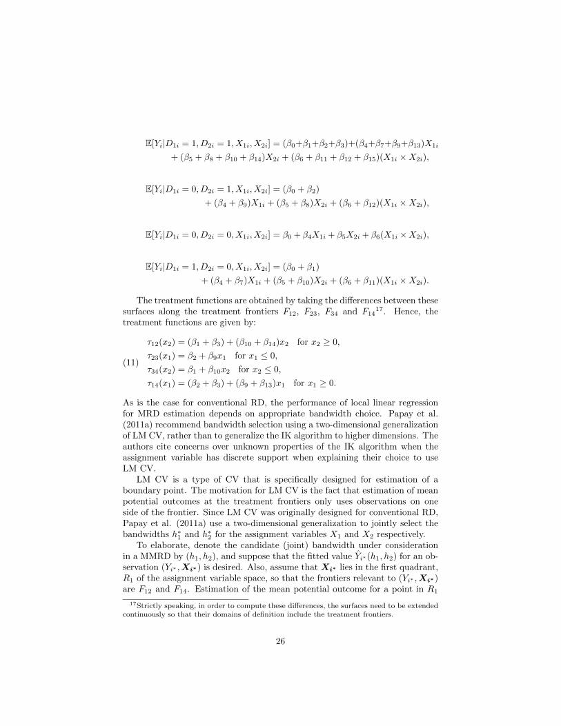
E[Yi|D1i = 1, D2i = 1, X1i, X2i] = (β0+β1+β2+β3)+(β4+β7+β9+β13)X1i

+ (β5 + β8 + β10 + β14)X2i + (β6 + β11 + β12 + β15)(X1i ×X2i),

E[Yi|D1i = 0, D2i = 1, X1i, X2i] = (β0 + β2)

+ (β4 + β9)X1i + (β5 + β8)X2i + (β6 + β12)(X1i ×X2i),

E[Yi|D1i = 0, D2i = 0, X1i, X2i] = β0 + β4X1i + β5X2i + β6(X1i ×X2i),

E[Yi|D1i = 1, D2i = 0, X1i, X2i] = (β0 + β1)

+ (β4 + β7)X1i + (β5 + β10)X2i + (β6 + β11)(X1i ×X2i).

The treatment functions are obtained by taking the differences between thesesurfaces along the treatment frontiers F12, F23, F34 and F14

17. Hence, thetreatment functions are given by:

(11)

τ12(x2) = (β1 + β3) + (β10 + β14)x2 for x2 ≥ 0,

τ23(x1) = β2 + β9x1 for x1 ≤ 0,

τ34(x2) = β1 + β10x2 for x2 ≤ 0,

τ14(x1) = (β2 + β3) + (β9 + β13)x1 for x1 ≥ 0.

As is the case for conventional RD, the performance of local linear regressionfor MRD estimation depends on appropriate bandwidth choice. Papay et al.(2011a) recommend bandwidth selection using a two-dimensional generalizationof LM CV, rather than to generalize the IK algorithm to higher dimensions. Theauthors cite concerns over unknown properties of the IK algorithm when theassignment variable has discrete support when explaining their choice to useLM CV.

LM CV is a type of CV that is specifically designed for estimation of aboundary point. The motivation for LM CV is the fact that estimation of meanpotential outcomes at the treatment frontiers only uses observations on oneside of the frontier. Since LM CV was originally designed for conventional RD,Papay et al. (2011a) use a two-dimensional generalization to jointly select thebandwidths h∗1 and h∗2 for the assignment variables X1 and X2 respectively.

To elaborate, denote the candidate (joint) bandwidth under considerationin a MMRD by (h1, h2), and suppose that the fitted value Yi∗(h1, h2) for an ob-servation (Yi∗ ,Xi∗) is desired. Also, assume that Xi∗ lies in the first quadrant,R1 of the assignment variable space, so that the frontiers relevant to (Yi∗ ,Xi∗)are F12 and F14. Estimation of the mean potential outcome for a point in R1

17Strictly speaking, in order to compute these differences, the surfaces need to be extendedcontinuously so that their domains of definition include the treatment frontiers.

26

arbitrarily close to these treatment frontiers will typically only use points tothe “north” or “east” of it. Therefore, in order to mimic the estimation of aboundary point, instead of using all points that are “close” to (Yi∗ ,Xi∗) in theassignment variable space,

{(Yj ,Xj) : |X1j −X1i∗ | ≤ h1 and |X2j −X2i∗ | ≤ h2} \ {(Yi∗ ,Xi∗)}

to estimate Yi∗(h1, h2) as one might do for standard CV, only points that are“close” to (Yi∗ ,Xi∗) and to the “northeast” of (Yi∗ ,Xi∗) are used, i.e.

{(Yj ,Xj) : 0 ≤ X1j−X1i∗ ≤ h1 and 0 ≤ X2j−X2i∗ ≤ h2} \ {(Yi∗ ,Xi∗)}.

To simplify notation, denote this set by Si∗(h1, h2). The following plotclarifies this concept by considering four points – one in each quadrant of theassignment variable space – and the regions determining Si(h1, h2) for eachpoint according to this bandwidth selection procedure.

After determining Si∗(h1, h2) for observation (Yi∗ ,Xi∗) for a given band-width, the fitted value for this point, Yi∗(h1, h2), is obtained via a linear regres-sion that only uses points in Si∗(h1, h2)18. To be explicit, one first estimatesthe OLS regression

(12) Yi = γ0 + γ1X1i + γ2X2i + γ3(X1i ×X2i) + ε

for (Yi,Xi) ∈ Si∗(h1, h2),

and then obtains the fitted value for (Yi∗ ,Xi∗) using the formula

(13) Yi∗(h1, h2) = γ0 + γ1X1i∗ + γ2X2i∗ + γ3(X1i∗ ×X2i∗).

The MSE for each candidate bandwidth (h1, h2)

(14) MSE(h1, h2) =1

N

N∑i=1

(Yi(h1, h2)− Yi)2

is calculated, and the bandwidth resulting in the lowest MSE is chosen as theoptimal bandwidth (h∗1, h

∗2).

Finally, the local linear regression is estimated using the subset of observa-tions

{(Yi,Xi) : |X1i| ≤ h∗1 or |X2i| ≤ h∗2}.18The procedure described in this section uses a rectangular kernel (i.e. OLS regression),

as Papay et al. do, for simplicity of exposition. The estimation can easily be modified toaccommodate other kernel choices, by using a weighted least squares regression with weightsthat depend on the choice of kernel. Two other popular choices of kernel (triangular andEpanechnikov) were discussed in the previous section on graphical analysis. An applicationof local linear estimation for MMRD that does not use a rectangular kernel can be found inSnider and Williams (2015). Incidentally, Snider and Williams mention in a footnote thattheir attempt at bandwidth selection via cross-validation was unsuccessful, without providingdetails about their implementation method.

27

●

●

●

●

X1

X2

h1

h2

Figure 7: This figure shows the regions (shaded rectangles) determiningSi(h1, h2) for four (solid black) points, as defined by the bandwidth selectionprocedure described in Papay et al. (2011a). In addition to the candidate band-width (h1, h2), the set of observations that are used to estimate the fitted valueof a point is also determined by the specific treatment region that the point liesin. The determination of the inclusion or exclusion of a side of the rectangle inthe relevant region reflects how the treatment conditions are defined along thetreatment frontiers.

28

4.2.2 MDRD Estimation via Local Linear Regression

While the estimation approach by Papay et al. (2011a) that I just described ismeant for MMRD (with four treatments), it can easily be modified for MDRD.In particular, there is no reason to revise the bandwidth selection procedurefor MDRD, so the only change needed is to tweak the local linear regressionfunction appropriately19.

I retain notation introduced earlier in the text, so that the dummy variablefor receiving treatment in MDRD is Wi = D1i×D2i. The local linear regressionequation for MDRD is thus:

(15) E[Yi|X1i, X2i] = β0 + β1Wi + β2X1i + β3X2i

+ β4(X1i ×X2i) + β5(Wi ×X1i) + β6(Wi ×X2i) + β7(Wi ×X1i ×X2i).

This regression equation results in the following two discontinuous linearsurfaces, the first being defined over the non-negative quadrant R1, and thesecond being defined over the rest of the assignment variable space R2∪R3∪R4:

E[Yi|Wi = 1, X1i, X2i] = (β0 + β1)

+ (β2 + β5)X1i + (β3 + β6)X2i + (β4 + β7)(X1i ×X2i),

E[Yi|Wi = 0, X1i, X2i] = β0 + β2X1i + β3X2i + β4(X1i ×X2i).

The treatment functions are obtained by taking the differences between thesesurfaces along the treatment frontiers F1 and F2, i.e. the non-negative x1- andx2-axes20. Hence, the treatment functions are given by:

(16)τ1(x2) = β1 + β6x2 for x2 ≥ 0,

τ2(x1) = β1 + β5x1, for x1 ≥ 0.

The subset of points used for this local linear regression is

{(Yi,Xi) : |X1i| ≤ h∗1 or |X2i| ≤ h∗2}∩{(Yi,Xi) : X1i ≥ −h∗1 and X2i ≥ −h∗2}.

4.2.3 Advantages and Disadvantages of Local Linear Regression forMRD Estimation

Some advantages of local linear regression for boundary estimation (based onthe estimator’s asymptotic properties) were mentioned earlier in this paper.

19This change in the regression function is required due to differences in the treatmentfrontiers for MDRD and MMRD. Specifically, the union of the treatment frontiers (F12 ∪F23 ∪ F34 ∪ F14) for the latter comprises of the entire x1- and x2-axes, so the regressionfunction allows for discontinuities along all of the two axes. By contrast, the union of thetreatment frontiers for the latter (F1 ∪F2) comprises of only the non-negative part of the twoaxes, so it would not make sense for the regression function to be discontinuous along thenegative parts of the axes (since there is no treatment effect to be estimated there). The locallinear regression function that I introduce for MDRD ensures that the regression function isonly allowed to be discontinuous along the treatment frontiers F1 and F2.

20As in the case for MMRD, in order to compute these differences, the surfaces need to beextended continuously so that their domains of definition include the treatment frontiers.

29

Another advantage of this approach is that the standard regression outputs –the estimated coefficients and their covariance matrix – are very convenient forhypothesis testing.

For instance, consider a MDRD estimation, and denote the vector of coeffi-cient estimates and its covariance matrix respectively by β and Σ (with rows andcolumns indexed from 0 to 7, in order to match the indices of the coefficients).For simplicity of exposition, assume that the error term is normally distributed.To obtain point-wise confidence intervals for the treatment function, I first de-note, for a given value of x2 ≥ 0, the random variable representing the treatmenteffect estimate at the point by T , and express the estimated treatment effect as

τ1(x2) = c′β, where c′ = [0 1 0 0 0 0 x2 0].

The (approximate) distribution of T is thus given by T ∼ N(c′β, c′Σc)21, whichallows for easy hypothesis testing of whether the estimated treatment functionat a given point is statistically different from zero (at a specified significancelevel).

Another hypothesis test of interest is whether there is statistical evidence ofa non-constant treatment effect. In this example, the hypothesis test amountsto whether the confidence interval for β6 contains zero, which is trivial since theestimated coefficient is (approximately) normally distributed and its variance is

given in the regression output as Σ6,6.

However, the attractive theoretical properties of estimation via local linearregression are predicated on appropriate bandwidth choice. In practice, the taskof selecting a suitable bandwidth has been a real difficulty which has not evenbeen fully resolved for conventional RD. The uncertainty over bandwidth choiceis exacerbated in MRD since the bandwidths for multiple assignment variablesmust be jointly selected, making this a multidimensional problem.

The bandwidth selection procedure just described is unsatisfactory in variousways. As LM (2005) themselves point out, CV estimates of the loss function aretypically relatively flat. LM take this as an indication of a more general prob-lem, that asymptotic properties of CV methods imply extremely slow rates ofconvergence. Moreover, the CV procedure documented by Papay et al. (2011a)has several other shortcomings, which I discuss below.

The first concerns a technical issue that the earlier description glosses over.The problem is that for a candidate bandwidth (h1, h2), the set of observationsSi∗(h1, h2) that are used to obtain a fitted value for (Yi∗ ,Xi∗) may not con-tain enough observations with unique combinations of the Xi to fit the linearregression, so that predicted values for these points may be undefined22. While

21This distributional result is only an approximation because β follows a t-distribution,rather than a normal distribution. However, this approximation is likely to be good even formoderate sample sizes.

22In fact, this will always be the case for points. For instance, consider the point Xi in thenon-negative quadrant R1 with the largest values of X1i and X2i. By definition, there are nopoints to the northeast of this particular point, and thus, Si(h1, h2) is empty.

30

Papay et al. (2011a) do not mention this problem in their discussion, I take theapproach of discarding these points and computing the MSE over the remainingpoints23.

Second, as pointed out by IK (2011), this procedure implicitly selects abandwidth that is optimal for fitting the mean regression function over the entireassignment variable space, rather than simply close to the treatment frontiers.To see why this may be problematic, consider an example where there is a greaterdensity of observations near the treatment frontiers than further away, anddenote the true optimal bandwidth by (hopt1 , hopt2 ). The sparse points that arefar away from the treatment frontier may in fact cause the procedure describedby Papay et al. to select a bandwidth (h∗1, h

∗2) that is larger than (hopt1 , hopt2 ).

This is because the true optimal bandwidth (hopt1 , hopt2 ) for estimation at thetreatment frontiers is too small for these points (due to the sparseness of pointsin their neighborhoods), leading to the selection of a larger bandwidth as acompromise. Heteroskedasticity may also result in a biased bandwidth choice.

Third, the bandwidth selection procedure is computationally expensive. Foreach candidate bandwidth (h1, h2), the algorithm involves a loop over all obser-vations in the dataset. Within this loop, for each observation i, the algorithmmust determine Si(h1, h2), fit a local linear regression using points in this set andobtain the fitted value Yi(h1, h2). Moreover, the number of potential bandwidthchoices is large, since the search for an optimal bandwidth is being conductedon a multidimensional grid.

4.2.4 Generalization of Bandwidth Selection Procedure described inPapay et al. (2011a)

In order to mitigate some of these problems, I propose a modification of the CVprocedure described in Papay et al. (2011a). In fact, the method I propose is amore general version of the CV procedure just discussed, and is closer in spiritto the original LM CV approach for conventional RD.

The original method implemented in LM (2005) does not compute the MSEover all points, as Papay et al. (2011a) do. Instead, only observations within fivepercentage points of either side of the cutoff are used for bandwidth selection. IK(2011) consider a slight generalization of LM CV by introducing an additional

23It is not obvious that discarding points for which fitted values cannot be obtained (for agiven candidate bandwidth) is the “right” thing to do. Consider a point that does not have“extreme” values of X1i and X2i (e.g. not in the northeast corner of R1, the northwest cornerof R2, and so forth), and suppose that there are insufficiently many points in Si(h1, h2) toestimate its fitted value. This is in fact a sign that for this point at least, the candidatebandwidth is “too small”. Hence, by ignoring such points when computing MSE, usefulinformation for bandwidth choice is lost.

One possible way to deal with this issue is to incorporate a penalty term for points whichhave undefined fitted values, and to modify the criterion function (currently the MSE), tobe a linear combinations of the sum of squared errors and the penalty term. However, thisintroduces another layer of complexity into a bandwidth selection procedure that is alreadyrather computationally burdensome, and does not address the method’s other shortcomingsmentioned in the text.

31

parameter δ which specifies the percentage of points to use on either side of thecutoff for bandwidth selection.

This idea of using only a proportion of points close to the threshold forbandwidth selection does not extend neatly to MRD. For instance, suppose onedecides to use δ percent of the points in R1 that are close to the treatmentfrontiers. Since there are two relevant frontiers for this region (the non-negativex1- and x2- axes), it is not obvious how to devise an objective method thatallocates this limited quota of points “fairly” between regions in R1 close toeach frontier, as well as along each frontier.

Therefore, I take the approach of using the quantiles for each assignmentvariable in each of the four quadrants of the assignment variable space. Specif-ically, for a chosen δ ∈ (0, 1], I define the following quantiles:

• Let p1 and q1 be the δth quantiles of X1i and X2i respectively, for obser-vations in R1 (i.e. observations with D1i = 1 and D2i = 1).

• Let p2 and q2 be the (1−δ)th and δth quantiles of X1i and X2i respectively,for observations in R2 (i.e. observations with D1i = 0 and D2i = 1).

• Let p3 and q3 be the (1 − δ)th quantiles of X1i and X2i respectively, forobservations in R3 (i.e. observations with D1i = 0 and D2i = 0).

• Let p4 and q4 be the δth and (1−δ)th quantiles of X1i and X2i respectively,for observations in R4 (i.e. observations with D1i = 1 and D2i = 0).

For MMRD, the set of observations used for bandwidth selection is

4⋃k=1

({(Yi,Xi) : |X1i| ≤ |pk| and |X2i| ≤ |qk|} ∩Rk

).

For MDRD, the precise definition is slightly messier, although it is also thecase that only observations close to the treatment frontiers (as defined by pkand qk) are used: (

{(Yi,Xi) : |X1i| ≤ |p1| or |X2i| ≤ |q1|} ∩R1

)⋃(

{(Yi,Xi) : X1i ≥ p2} ∩R2

)⋃(

{(Yi,Xi) : |X1i| ≤ |p3| and |X2i| ≤ |q3|} ∩R3

)⋃(

{(Yi,Xi) : X2i ≥ q3} ∩R4

).

While this parameter δ does not represent the proportion of points in eachtreatment region being used, it still controls the amount of data close to thetreatment frontiers that is used for bandwidth selection. For instance, the pro-cedure described in Papay et al. (2011a) that uses all observations correspondsto the special case of δ = 1.

32

By only using points that are “close” (“closeness” being controlled by δ)to the treatment frontiers for estimation, the problems mentioned above areameliorated to a certain extent. For suitably small choices of δ, observationsthat “too far” from the treatment frontiers are no longer used for bandwidthselection. Moreover, the computational burden for bandwidth selection is easedslightly since this method uses fewer observations.

However, this modification does not solve other problems with CV mentionedearlier. Furthermore, this method raises an additional question concerning thechoice of δ. Both LM and IK use subjective judgment to determine the pro-portion of data near the threshold to use. The lack of an objective method todetermine δ is especially problematic if the bandwidth selected by this approachturns out to be sensitive to the choice of δ.24

The discussion in this subsection reveals that, despite the attractive proper-ties of local linear regressions for boundary estimates, performance in practicecan be hampered by inappropriate bandwidth choice. Procedures for bandwidthselection suffer from various problems, which tend to be exacerbated when thesemethods are extended from conventional RD to MRD.

In light of these difficulties, this paper proposes a non-parametric methodfor MRD estimation that does not require bandwidth selection – thin plateregression splines. The method is closely related to thin plate splines, whichis the multidimensional analogue of a penalized spline method that Rau (2011)proposed for estimation in conventional RD. The next subsection covers MRDestimation via thin plate regression splines.

4.3 Thin Plate Regression Splines

A thin plate spline has various properties that make it attractive for MRD esti-mation. First, it is a local estimator (unlike global polynomials), which makesit less susceptible to boundary effects. Second, the flexibility of this methodallows for easy estimation of non-constant treatment effects. In particular, onedoes not need to specify a functional form for the treatment function estimate.Finally, it is far more convenient to fit than other popular local smoothing meth-ods. For instance, local linear regression and cubic splines require bandwidthand knot selection respectively, in order to control the smoothness of the fittedsurface (i.e. to avoid over-fitting or over-smoothing). In the context of MRD,both bandwidth and knot selection require a grid search in multiple dimensions,

24One possible way to choose δ objectively is to treat δ as an additional tuning parameter,and jointly determine the optimal bandwidth as well as δ using the CV method just described.Unfortunately, in addition to imposing significant additional computational burden (since theinclusion of δ as a tuning parameter adds yet another dimension to the grid search for optimalparameter values), this approach may not yield a good choice of δ or bandwidth. For instance,suppose that “irrelevant” points that are far from the treatment frontiers come from a data-generating process that is much closer to linear than for points closer to the frontiers. Includingthese “irrelevant” points may reduce MSE significantly, so the resulting choice of δ is largerthan optimal. Hence, even when δ is used as a tuning parameter, “irrelevant” observationsfar from the frontiers can have substantial influence on bandwidth selection.

33

which can be computationally expensive. By contrast, the smoothness of thinplate splines is controlled by a single scalar tuning parameter.

4.3.1 Thin Plate Splines

The concept of thin plates splines is first introduced in Duchon (1977), and islater revisited in Wood (2003) and Wood (2006). A thin plate spline seeks toestimate a function of multiple variables from noisy data, with the smoothnessof this function being controlled by a penalty term. More formally, given Nobservations (yi,xi), xi ∈ Rd from a data-generating process

yi = g(xi) + εi,

where g is a smooth function and εi are random errors, the smoothing spline fiis the estimate of g that minimizes the following quantity:

(17)

N∑i=1

(yi − f(xi))2 + λJmd(f).

This minimand is the sum of a loss function and a penalty term, with Jmd inthe penalty term defined by:

(18) Jmd ≡∫...

∫Rd

∑ν1+...+νd=m

m!

ν1!...νd!

(∂mf

∂xν11 ...xνdd

)2

dx1...dxd.

The choice of m is required to satisfy 2m > d , although typically 2m > d + 1is also respected so that the estimated function is “visually smooth”. If one isdealing with two assignment variables (d = 2), then m = 2 would be a goodchoice, in which case the penalty term is:

J22 =

∫ ∫ (∂f

∂x21

)2

+ 2 ·(

∂f

∂x1∂x2

)2

+

(∂f

∂x22

)2

dx1dx2.

The coefficient on the penalty term, λ, is a tuning parameter that is typicallychosen by generalized cross-validation (GCV), which is a modification to an-other popular choice – leave-out-out-cross-validation (LOOCV). GCV is oftenpreferred to LOOCV because it is less computationally expensive, and is invari-ant to rotation of the outcome vector and basis matrix25.

25In fact, the popularity of LOOCV (relative to k-fold cross-validation for instance) is alsopartly due to computational reasons. It turns out that instead of fitting N different modelsto find the LOOCV score for a particular choice of λ, there is an easy formula which onlyrequires a single model fit,

LOOCV (λ) =1

N

N∑i=1

[yi − (Ay)i]2

(1−Aii)2,

where A is the influence matrix for the model fit using λ (so that A is actually a function ofλ, although the notation does not reflect this). The GCV score is given by a similar formula:

GCV (λ) =N ||y −Ay||2

[N − tr(A)]2.

34

4.3.2 Thin Plate Regression Splines

Despite the advantages of thin plate splines outlined at the start of this sub-section, a major disadvantage is its computational cost, which remains a majorobstacle to its widespread use in practical statistical work. At present, thinplate splines are most commonly used in the special case of d = 1 (where themethod is known by a number of different names such as “penalized splines”or “smoothing splines”) since there exists an efficient algorithm for this specialcase26. Denoting the number of unique combinations of covariate values by n(which may be smaller than the total number of observations N due to discretemeasurements of data), the computational cost for penalized splines is on theorder of O(n) as opposed to O(n3) for the general case. Hence, the primary mo-tivation for the construction of thin plate regression splines (henceforth TPRS)is to provide a relatively computationally inexpensive alternative to thin platesplines.

A major reason for the computational expense in fitting thin plate splinesis that the basis matrix is of rank n. Yet, this seems “wasteful” in the sensethat the effective degrees of freedom27 tends to be a small proportion of n. Theidea behind TPRS is to approximate thin plate splines using a low rank basismatrix (of say, rank k), obtained by truncating the most “wiggly” componentsof the thin plate spline (which were penalized heavily anyway in the thin platespline fit), while leaving those components with “zero wiggliness” untouched28.This modification results in significant computational cost savings – the cost offitting a TPRS is at most O(kn2), as opposed to O(n3) for thin plate splines.Moreover, the computationally costly model selection algorithm is only O(k2n)for TPRS, compared to O(n3) for thin plate splines.

When fitting a TPRS, one must choose the basis dimension k, in addition tothe smoothness parameter λ, so it may seem that tuning the model for TPRSis more tedious than for thin plate splines. However in practice, for a givenvalue of k, the actual effective degrees of freedom is controlled by λ. So, thechoice of k is not critical as long as it is chosen large enough so that the modelis not overly restricted by the basis dimension (i.e. k should be chosen to belarger than the effective degrees of freedom believed to be required). Kim andGu (2004) show that basis dimension should scale as n2/9, and suggest 10n2/9

based on simulations. The appendix in this paper provides an example exploringthe sensitivity of TPRS treatment effect estimates to the choice of k.

Standard errors for the model parameters in TPRS can be derived usinga Bayesian approach to uncertainty estimation, assuming a fixed value of thesmoothing parameter λ.29 If the error term in the data-generating process isnormal, then the posterior distribution of the model parameters is multivari-ate normal. Otherwise, approximate normality of the posterior distribution is

26Rau (2011) discusses an estimation approach for conventional RD using penalized splines(i.e. thin plate splines with d = 1).

27The effective degrees of freedom is defined as the trace of the influence matrix.28Interested readers should refer to the appendix for additional details on the approximation

of thin plate splines by TPRS.29Readers may refer to Wood (2006) for a derivation of this result.

35

justified by large sample theory.

4.3.3 MRD Estimation via TPRS

MRD estimation via TPRS is easy to implement. First, one would fit a sepa-rate TPRS for observations in each treatment region in the assignment variablespace. Point estimates of the treatment effect along each treatment frontier canthus be obtained by taking the difference between fitted values (from the twoTPRS functions estimated using data in the two adjacent treatment regions).

To avoid any ambiguity, I explicitly state the formulae for the estimatedtreatment effect functions, starting with those for MDRD. Denote the fittedTPRS functions by f1(x1, x2) and f0(x1, x2), these being the estimates of

E[Y (1)|X1 = x1, X2 = x2)] and E[Y (0)|X1 = x1, X2 = x2)],

using data from R1 and R2 \ R1 respectively. The MDRD treatment effectestimates are thus given by:

(19)τ2(x2) ≡ f1(0, x2)− f0(0, x2) for x2 ≥ 0,

τ2(x1) ≡ f1(x1, 0)− f0(x1, 0) for x1 ≥ 0.

Next for MMRD, I denote the fitted TPRS functions for observations in regionsR1, R2, R3 and R4 respectively by f1, f2, f3 and f4. Using this notation, thetreatment effect estimates for MMRD can be expressed as:

(20)

τ12(x2) ≡ f1(0, x2)− f2(0, x2) for x2 ≥ 0,

τ23(x1) ≡ f3(x1, 0)− f2(x1, 0) for x1 ≤ 0,

τ34(x2) ≡ f4(0, x2)− f3(0, x2) for x2 ≤ 0,

τ14(x1) ≡ f1(x1, 0)− f4(x1, 0) for x1 ≥ 0.

Approximate Bayesian confidence intervals for the point estimates of thesetreatment effect functions can be obtained using the posterior distributions ofpoint estimates from the fitted TPRS functions. For concreteness, I take theestimation of τ1(x2) in MDRD as an example, although the procedures forτ2(x1) as well as for MMRD are completely analogous. Following the Bayesianframework, I consider the parameters

f1(0, x2) = E[Y (1)|X1 = 0, X2 = x2)] and f0(0, x2) = E[Y (0)|X1 = 0, X2 = x2)]

as random variables, which I denote by V1 and V0 respectively. This yields

V1 ∼ N(f1(0, x2), σ21) and V0 ∼ N(f0(0, x2), σ2

0),

where the moments of these normal distributions are known. It follows that

V1 − V0 ∼ N(f1(0, x2)− f0(0, x2), σ2),

36

where σ2 = σ21 + σ2

0 − 2Cov(V1, V0). Although the value of Cov(V1, V2) isunknown, an upper bound for σ2 can still be found by using the inequalityCov(V1, V0) ≥ −σ1σ0, so that a conservative Bayesian confidence interval forτ1(x2) may be obtained.

On the other hand, the assumption of maximum negative covariance betweenV1 and V0 may be too pessimistic. One may think that the correlation betweenexpected potential outcomes at any point on the frontier should be positive.Hence, a more optimistic confidence interval may be obtained by assuming zerocovariance (and hence independence, due to normality) between V1 and V0.30

Hence, to recap the discussion about point-wise confidence intervals for treat-ment effect estimates along the frontiers, one may either use a conservativeBayesian confidence interval which assumes, for τ1(x2) in a MDRD, that

V1 − V0 ∼ N(f1(0, x2)− f0(0, x2), (σ1 + σ0)2),

or a more optimistic confidence interval which assumes

V1 − V0 ∼ N(f1(0, x2)− f0(0, x2), σ21 + σ2

0).

5 Simulation

In this section, I conduct an extensive simulation study based closely on theNBER paper by Kane (2003). Methods for graphical analysis and estimationdescribed earlier in this paper are demonstrated, and the strengths and weak-nesses of each approach assessed.

5.1 Background on Original Paper

The design of this simulation study is based on the NBER paper by Kane(2003), titled “A Quasi-Experimental Estimate of the Impact of Financial Aidon College-Going”. The paper investigates how the CalGrant program affectedcollege going rates in California from 1998 to 1999 using a sharp regression-discontinuity design. Eligibility for the CalGrant A program required that theapplicant’s high school GPA, parental income and asset (excluding home equity)satisfy certain cutoff rules for each of these variables31. The number of awardseach year was fixed, so the GPA cutoff (which ultimately depended on the num-ber of eligible applicants) was unknown at the time of application. This makeshigh school GPA a particularly suitable assignment variable since it cannot bemanipulated precisely, thus ensuring that students’ GPAs near the thresholdare as-good-as-random.

30In fact, the optimistic confidence interval occupies the middle ground between the mostpessimistic and optimistic assumptions about Cov(V1, V0). Strictly speaking, the most op-timistic assumption is that V1 and V0 are perfectly positively correlated, but such heroicassumptions are not typically adopted for inference.

31There were actually two CalGrant programs (CalGrant A and B), but Kane focuses mainlyon estimating the impact of CalGrant A on college going.

37

Since there are multiple assignment variables (GPA, income and assets) andtwo mutually exclusive treatment conditions (eligibility/ineligibility for the Cal-Grant program), this is a MDRD problem. Kane takes the “univariate” ap-proach, estimating the treatment effects separately along each frontier. Hefocuses mostly on the GPA threshold, where he finds approximately a threepercent increase in college going rate for applicants whose GPAs just pass thethreshold, relative to those whose GPAs just miss in 1998. Kane also considersthe income and asset thresholds, but for the most part, does not find statisti-cally significant effects (possibly due to there being an insufficient number ofobservations near these thresholds, especially for the asset threshold).

5.2 Generating the Simulated Dataset

Unfortunately, the original data for Kane’s paper is no longer available, so Icreate simulated dataset that is similar to the original one based on summarystatistics and estimation results reported in the paper. Following the paper, Ifocus on estimating the impact that CalGrant A eligibility had on college goingrates in 1998. My assignment variables are high school GPA and income, sincethe original paper hardly presented any results for the asset threshold.

First, I generate the assignment variables so that their distributions approx-imate those in the original paper. For high school GPA, I chose a scaled, shiftedand truncated beta distribution which is similar to the empirical distributionin Kane’s paper. The income threshold varies for families of different sizes, soI assume that the incomes for families of various sizes each follow a lognormaldistribution with separate means, choosing the proportions of different familysizes so that the mean family size is close to that reported in the paper32. Ithen restrict the data to observations with GPA between 2.50 and 3.60 andexclude applicants who were eligible for both Cal Grants A and B, using thisreduced sample for all subsequent analysis, following Kane’s paper. The num-ber of observations as well as the mean and median of assignment variables inthe reduced sample are very similar to those reported for the original data. Ithen shift and rescale the variables so that they are centered at zero, with thenon-negative quadrant of the assignment variable space, R1 corresponding toeligibility for the program. Histograms for the simulated covariate values in thereduced sample are shown below.

Next, I select by trial-and-error, two data-generating processes (DGPs) togenerate the outcome variable (college going). In particular, I made sure thatthe mean college going rate in the simulated data, as well as the regression resultsobtained by applying Kane’s estimation approach for the GPA threshold to mydata, are similar to those presented in the paper. I focus on replicating Kane’sestimation results for the GPA threshold for two main reasons – first, Kane’sregressions for the GPA and income thresholds are incomparable; second, hisregression results for the GPA threshold are much stronger. To elaborate, Kane

32Clementi and Gallegati (2005) document that the empirical income distribution for thebottom 97 to 99 percent of the population (which encompasses the population of interest forKane’s paper) is consistent with lognormal distribution.

38

Histogram of X1

X1

Fre

quen

cy

−0.6 −0.4 −0.2 0.0 0.2 0.4

020

040

060

080

010

0012

00

Histogram of X2

X2

Fre

quen

cy

−100 −80 −60 −40 −20 0 20 40

010

0020

0030

0040

00

Figure 8: Histograms of the simulated assignment variables after restricting thedata following Kane’s approach.

estimates regressions for the GPA threshold with and without other covariates,using the subsamples of observations in 1998 and 1999 separately. For theincome threshold, Kane instead estimates a regression using the pooled sampleof observations from both years, with the inclusion of covariates. Yet, even usinga pooled sample and including other covariates to increase precision, Kane’sestimate for the income threshold is insignificant at the 5 percent level and hasa higher p-value than the estimate at the GPA threshold using the 1998 samplealone without the inclusion of other covariates. Moreover, there is insufficientinformation about the covariates included in his income threshold regression tosimulate these variables realistically. Hence, it likely would have been a fruitlesstask to attempt a reasonable replication of Kane’s estimates on the incomethreshold.

Next, I describe the two DGPs I chose. Denoting the indicator for collegegoing by

Y ≡ I[Entered College in the Next Year],

the general form for the DGP is

Pr(Y = 1|X1, X2) = α0 + α1X1 + α2X21 + α3X

31 + α4X2 + α5X

22 + α6X

31+

α7X1X2 + α8X21X2 + α9X1X

22 + α10sin(X1) + α11sin(X2)+

Wi · (g(X1) + h(X2)),

39

where

X1 ≡ (High School GPA)− (1998 GPA Cutoff),

X2 ≡ −1

1000· (Family Income− Income Cutoff), and

α0 = 0.82, α1 = 0.1, α2 = −0.01, α3 = −0.01, α4 = −2 · 10−4,

α5 = −10−6, α6 = −10−7, α7 = 10−6, α8 = −10−6, α9 = 10−6,

α10 = 0.01, α11 = 0.01.

For the first DGP, I assume constant treatment effect along both frontiers,setting

g(X1) = h(X2) = 0.025 for all X1 and X2,

whereas for the second process, non-constant treatment effects are assumed,with

g(X1) = 0.15 ∗[Φ

(X1

0.25

)− 0.5

]and h(X2) = 0.06 ∗

[Φ

(X2

15

)− 0.5

],

where Φ denotes the cumulative distribution function of a standard normalrandom variable.

Using these probabilities, I generate the outcome variable Y correspondingto the simulated assignment variables. As with the assignment variables, themean value of simulated outcomes is similar to the mean in the original data.

For estimation at the GPA threshold, Kane uses a probit regression with acubic polynomial in high school GPA and a dummy variable indicating whetherGPA passes the threshold. The DGPs were chosen so that running the sameregression on the simulated datasets produces results similar to Kane’s. Thefollowing regression table shows estimates for the marginal impact of crossingthe GPA threshold on probability of college going. The point estimates andstandard errors from the original paper are similar to those obtained using thesimulated datasets, and the estimated treatment effect is significant at the 10percent level in all three columns33.

The next plots display the DGPs I chose for the constant and non-constanttreatment effects respectively. Two features of these DGPs would seem to favorestimation via local linear regression over estimation via TPRS (although itturns out that TPRS still outperforms probit and local linear estimates onthese simulated datasets).

First, the plots clearly show that the DGPs exhibit sinusoidal behavior, es-pecially along the X2 direction (which corresponds to income)34. These periodic

33Kane’s paper does not include other statistics from the regression other than sample size.34In fact, the DGP also includes periodic behavior in the X1 direction (which corresponds

to GPA). However, due to the scaling of the assignment variables, only the periodic behaviorin the income direction is obvious. This is because the period of an oscillation in both the X1

and X2 direction is 2π, whereas the ranges of X1 and X2 in the plots are from −0.4 to 0.4and −30 to 30 respectively.

40

Table 1: Probit Regression for GPA Threshold

Dependent variable:

College Going

Kane’s Data Simulated Data Simulated Data(Constant Treat) (Non-Constant Treat)

I[X1 ≥ 0] 0.029∗ 0.033∗ 0.030∗

(0.015) (0.017) (0.016)

Observations 11,750 11,750 11,750Order of Polynomial 3 3 3in GPA

Note: ∗p<0.1; ∗∗p<0.05; ∗∗∗p<0.01

terms were included in the DGP to test the robustness of the TPRS treatmenteffect estimate. In particular, the true treatment effect along the GPA thresh-old – being the difference between the discontinuous surfaces along F1 – is notperiodic because the sinusoidal behavior at the boundaries of the two surfacescancel out. However, the TPRS surfaces are unlikely to fit this periodic behav-ior perfectly, so that the TPRS estimate – being the difference between the twodiscontinuous TPRS surfaces – may still exhibit some periodic behavior which isnot canceled out in the difference35. By contrast, the true DGP hardly exhibitsany periodic behavior along the income threshold, so one may expect the TPRSestimate to perform better along this threshold.

Second, periodic terms aside, the DGP is a cubic polynomial in X1 and X2,with the quadratic, cubic and interaction coefficients largely dominated by thelinear coefficients on X1 and X2. Hence, one would expect that local linearestimate to perform well given that the DGP is “close to linear”.

5.3 Graphical Analysis with the Simulated Data

In this subsection, I demonstrate several graphical analysis methods describedin section 3 using the simulated dataset with non-constant treatment effects.In particular, I show the outcome discontinuity plots for the GPA and incomethresholds created using the “slicing” approach with a linear regression line fitto observations on each side of the cutoff, as well as the corresponding “slidingwindow” plots for the two cutoffs. In the “sliding window” graphs, I overlay thetrue DGP for comparison (using the true probabilities of college going arbitrarilyclose to each cutoff). Of course, lines representing the DGP would be absent in“sliding window” plots for a real dataset (where the DGP is unknown).

35This periodic behavior has a less pronounced effect on the probit and local linear estimates,since these methods are less flexible than the TPRS approach.

41

Figure 9: Data-generating processes for the simulated datasets.

42

●

●

●

●

●●

●

●

●

●

●

●

−0.6 −0.4 −0.2 0.0 0.2 0.4

0.70

0.80

0.90

1.00

Applicants with ParentalIncome $0−$9,999 Below Cutoff

2442 Applicants

GPA−cutoff

Col

lege

Goi

ng R

ate

●

●

●

●

●●

●

●

●●

●

●

−0.6 −0.4 −0.2 0.0 0.2 0.4

0.70

0.80

0.90

1.00

Applicants with ParentalIncome $10,000−$19,999 Below Cutoff

3278 Applicants

GPA−cutoff

Col

lege

Goi

ng R

ate

●

●

●

●

● ●●

●

●

●

●●

−0.6 −0.4 −0.2 0.0 0.2 0.4

0.70

0.80

0.90

1.00

Applicants with ParentalIncome $20,000−$29,999 Below Cutoff

4396 Applicants

GPA−cutoff

Col

lege

Goi

ng R

ate

●

●

●

●●

●

●

●

●

●

●

●

−0.6 −0.4 −0.2 0.0 0.2 0.4

0.70

0.80

0.90

1.00

Applicants with ParentalIncome $30,000+ Below Cutoff

1634 Applicants

GPA−cutoff

Col

lege

Goi

ng R

ate

Figure 10: These “slicing” method plots show the discontinuity in college-goingrate at the GPA threshold for applicants with different levels of parental income.These graphs were created using the simulated dataset with non-constant treat-ment effect.

43

●

●

●

●

● ●

●

●

●

●

−10 0 10 20

0.70

0.80

0.90

1.00

Applicants with GPA 0−0.09 Above Cutoff

929 Applicants

− (Income − Cutoff)

Col

lege

Goi

ng R

ate

●

●

●

●

●●

●●

●

●

−10 0 10 20

0.70

0.80

0.90

1.00

Applicants with GPA 0.1−0.19 Above Cutoff

961 Applicants


Col

lege

Goi

ng R

ate

●

●●

●

●

●

● ●

●

●

−10 0 10 20

0.70

0.80

0.90

1.00


1103 Applicants


Col

lege

Goi

ng R

ate

●

●

●

●

●

● ●

● ●

●

−10 0 10 20

0.70

0.80

0.90

1.00


1062 Applicants


Col

lege

Goi

ng R

ate

Figure 11: These “slicing” method plots show the discontinuity in college-goingrate at the income threshold for applicants with different GPAs These graphswere created using the simulated dataset with non-constant treatment effect.

44

5 10 15 20 25

0.76

0.78

0.80

0.82

0.84

0.86

0.88

College Going Rates for Applicants Near the GPA Thresholdwith Different Parental Incomes

(Simulated Data with Non−Constant Treatment Effect)

X2 = − (Income − Cutoff)

Y =

Col

lege

Goi

ng R

ate

Applicants Just Below GPA ThresholdApplicants Just Above GPA ThresholdDGP Just Below GPA ThresholdDGP Just Above GPA Threshold

Figure 12: This “sliding window” plot shows the college-going rate for applicantswith different levels of parental income who are just below and just above theGPA threshold. The solid lines represent the actual “sliding window” plot, andthe dashed lines are the DGP for the simulated data, overlaid for comparison.Lines representing the DGP would be absent in “sliding window” plots for areal dataset (where the DGP is unknown). This graph was created using thesimulated dataset with non-constant treatment effect.

45

0.05 0.10 0.15 0.20 0.25 0.30 0.35 0.40

0.80

0.85

0.90

0.95

College Going Rates for Applicants Near the Income Thresholdwith Different GPA's

(Simulated Data with Non−Constant Treatment Effect)

X1 = (GPA − Cutoff)

Y =

Col

lege

Goi

ng R

ate

Applicants Just Above Income ThresholdApplicants Just Below Income ThresholdDGP Just Above Income ThresholdDGP Just Below Income Threshold

Figure 13: This “sliding window” plot shows the college-going rate for applicantswith different GPAs who are just below and just above the income threshold.The solid lines represent the actual “sliding window” plot, and the dashed linesare the DGP for the simulated data, overlaid for comparison. Lines representingthe DGP would be absent in “sliding window” plots for a real dataset (wherethe DGP is unknown). This graph was created using the simulated dataset withnon-constant treatment effect.

46

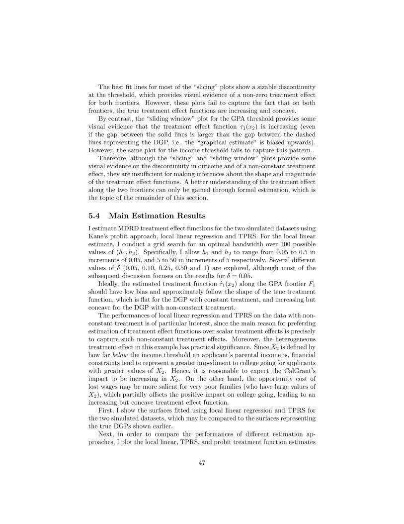
The best fit lines for most of the “slicing” plots show a sizable discontinuityat the threshold, which provides visual evidence of a non-zero treatment effectfor both frontiers. However, these plots fail to capture the fact that on bothfrontiers, the true treatment effect functions are increasing and concave.

By contrast, the “sliding window” plot for the GPA threshold provides somevisual evidence that the treatment effect function τ1(x2) is increasing (evenif the gap between the solid lines is larger than the gap between the dashedlines representing the DGP, i.e. the “graphical estimate” is biased upwards).However, the same plot for the income threshold fails to capture this pattern.

Therefore, although the “slicing” and “sliding window” plots provide somevisual evidence on the discontinuity in outcome and of a non-constant treatmenteffect, they are insufficient for making inferences about the shape and magnitudeof the treatment effect functions. A better understanding of the treatment effectalong the two frontiers can only be gained through formal estimation, which isthe topic of the remainder of this section.

5.4 Main Estimation Results

I estimate MDRD treatment effect functions for the two simulated datasets usingKane’s probit approach, local linear regression and TPRS. For the local linearestimate, I conduct a grid search for an optimal bandwidth over 100 possiblevalues of (h1, h2). Specifically, I allow h1 and h2 to range from 0.05 to 0.5 inincrements of 0.05, and 5 to 50 in increments of 5 respectively. Several differentvalues of δ (0.05, 0.10, 0.25, 0.50 and 1) are explored, although most of thesubsequent discussion focuses on the results for δ = 0.05.

Ideally, the estimated treatment function τ1(x2) along the GPA frontier F1

should have low bias and approximately follow the shape of the true treatmentfunction, which is flat for the DGP with constant treatment, and increasing butconcave for the DGP with non-constant treatment.

The performances of local linear regression and TPRS on the data with non-constant treatment is of particular interest, since the main reason for preferringestimation of treatment effect functions over scalar treatment effects is preciselyto capture such non-constant treatment effects. Moreover, the heterogeneoustreatment effect in this example has practical significance. Since X2 is defined byhow far below the income threshold an applicant’s parental income is, financialconstraints tend to represent a greater impediment to college going for applicantswith greater values of X2. Hence, it is reasonable to expect the CalGrant’simpact to be increasing in X2. On the other hand, the opportunity cost oflost wages may be more salient for very poor families (who have large values ofX2), which partially offsets the positive impact on college going, leading to anincreasing but concave treatment effect function.

First, I show the surfaces fitted using local linear regression and TPRS forthe two simulated datasets, which may be compared to the surfaces representingthe true DGPs shown earlier.

Next, in order to compare the performances of different estimation ap-proaches, I plot the local linear, TPRS, and probit treatment function estimates

47

0.40.2

Linear Surfaces fitted forSimulated Data with

Constant Treatment Effect

0

X1

-0.2-0.4-40

-20

X2

0

20

0.85

0.9

0.75

0.8

40

Pr(

Y=

1)

0.40.2

Linear Surfaces fitted forSimulated Data with

Non-Constant Treatment Effect

0

X1

-0.2-0.4-40

-20

X2

0

20

1

0.95

0.9

0.85

0.8

0.7540

Pr(

Y=

1)

Figure 14: Linear surfaces fitted for the simulated datasets using local linearregression.

48

0.40.2

TPRS Surfaces fitted forSimulated Data with

Constant Treatment Effect

0

X1

-0.2-0.4-40

-20

X2

0

20

0.85

0.9

0.75

0.8

40

Pr(

Y=

1)

0.40.2

TPRS Surfaces fitted forSimulated Data with

Non-Constant Treatment Effect

0

X1

-0.2-0.4-40

-20

X2

0

20

0.9

0.75

0.8

0.95

0.85

40

Pr(

Y=

1)

Figure 15: TPRS surfaces fitted for the simulated datasets.

49

for the GPA threshold on the same plots. Conservative 95 percent Bayesian con-fidence intervals (CIs) for the TPRS estimates, as well as the true treatmenteffects are also shown.

The plots for the estimated treatment functions along the GPA boundary F1

show that the TPRS estimate works reasonably well in practice. Its performanceon the GPA threshold is comparable to the probit regression, and far superior tothe local linear estimate. This is despite the TPRS estimates being affected (forthe worse) by the periodic behavior of the true DGPs near the GPA threshold(as evidenced by the plots showing the fitted TPRS surfaces).

In the plot for constant treatment effect, although the TPRS estimate isslightly wiggly, it does not exhibit an obvious increasing or decreasing trend,and its bias is similar to Kane’s probit regression approach. For the plot with anincreasing and concave treatment function, the TPRS estimate is also increasingand concave over most of F1. While the TPRS estimate is far from perfect (forinstance, it is biased upwards and its shape does not follow that of the truefunction exactly), its 95 percent CIs contain the true treatment function in bothplots. Moreover, for the data with non-constant treatment effect, the TPRS CIincludes zero for small values of X2 and excludes zero for most larger values ofX2. This is in line with the true treatment function, which starts at zero andincreases with X2. The precision of the TPRS estimates on the GPA thresholdis similar to that of the probit estimate – significant at the 10 percent level butnot always at the 5 percent level.

By contrast, the local linear regression tends to exhibit higher bias in bothplots, and its shape is totally uninformative about the shape of the true treat-ment function. In particular, as the linear surfaces and the treatment effectplots show, the local linear estimate is decreasing in X2 for both datasets, eventhough the true treatment functions are constant for the first dataset and in-creasing for the second.

Next, I consider estimation of the treatment effect along the income frontier.As mentioned earlier, Kane’s income threshold regressions are incomparable tohis GPA threshold regressions. Nonetheless, I estimate probit regressions for theincome threshold on the simulated datasets in the way that most closely followshis approach (i.e. with the same specification, except without other covariates,and using the 1998 subsample). The regression output and plots of the MDRDtreatment function estimates are shown below.36

36Strictly speaking, the blue line in the plot should not be constant in X1 because Kane’sprobit regression at the income threshold includes linear and quadratic terms in X1. Theconstant blue line represents the marginal effect of crossing the income threshold on theprobability of entering college when all the other covariates (including X1 and X2

1 ) are fixedat their mean. Hence, the blue line in a “correct” plot should be a non-constant functionof X1. Such a plot is shown in the appendix, where it is clear from the output that thevarying treatment effect predicted using the probit model is still relatively constant, andin fact, performs slightly worse. Since the goal is to compare the TPRS (and local linear)estimate to the best benchmark of the probit regression, none of the results in this paper willbe overstated by presenting a treatment effect for Kane’s probit model that is better thanit actually is. Hence, for simplicity sake (since standard errors for the marginal probit effect

50

0.000

0.025

0.050

0.075

0 10 20 30

X2

Trea

tmen

t Effe

ct

TPRSProbitLocal Linear

Estimated Treatment Effects(GPA Frontier, Constant Treatment Effect)

−0.025

0.000

0.025

0.050

0.075

0 10 20 30

X2

Trea

tmen

t Effe

ct


Estimated Treatment Effects(GPA Frontier, Non−Constant Treatment Effect)

Figure 16: The thick black line in these plots represents the true treatmenteffect at the GPA threshold for the simulated data. The blue line is the MDRDestimate using TPRS, the red line is the probit estimate using Kane’s approachand the dark green line is the local linear estimate with bandwidth selection viaLM CV using δ = 0.05. The shaded region represents the 95 percent conserva-tive Bayesian confidence intervals for the TPRS point estimates of the treatmentfunction.

51

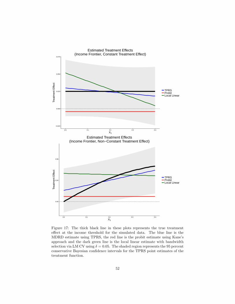
−0.025

0.000

0.025

0.050

0.075

0.0 0.1 0.2 0.3 0.4

X1

Trea

tmen

t Effe

ct


Estimated Treatment Effects(Income Frontier, Constant Treatment Effect)

0.00

0.04

0.08

0.0 0.1 0.2 0.3 0.4

X1

Trea

tmen

t Effe

ct


Estimated Treatment Effects(Income Frontier, Non−Constant Treatment Effect)

Figure 17: The thick black line in these plots represents the true treatmenteffect at the income threshold for the simulated data. The blue line is theMDRD estimate using TPRS, the red line is the probit estimate using Kane’sapproach and the dark green line is the local linear estimate with bandwidthselection via LM CV using δ = 0.05. The shaded region represents the 95 percentconservative Bayesian confidence intervals for the TPRS point estimates of thetreatment function.

52

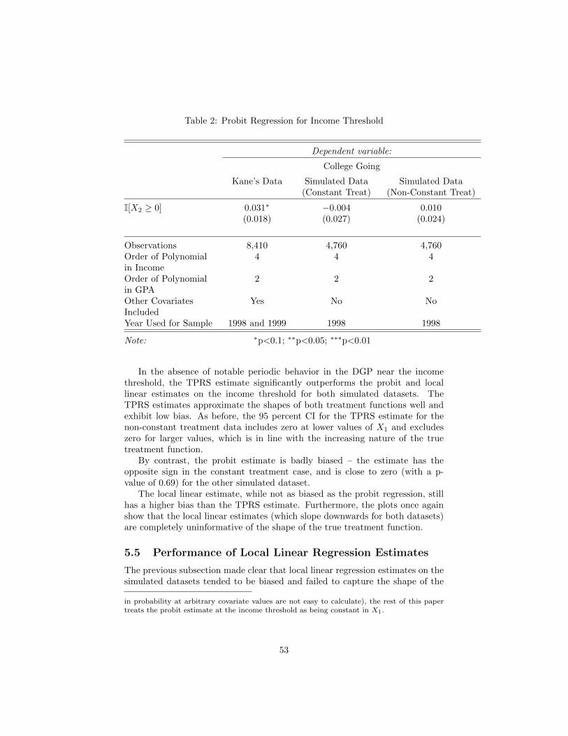
Table 2: Probit Regression for Income Threshold

Dependent variable:

College Going


I[X2 ≥ 0] 0.031∗ −0.004 0.010(0.018) (0.027) (0.024)

Observations 8,410 4,760 4,760Order of Polynomial 4 4 4in IncomeOrder of Polynomial 2 2 2in GPAOther Covariates Yes No NoIncludedYear Used for Sample 1998 and 1999 1998 1998

Note: ∗p<0.1; ∗∗p<0.05; ∗∗∗p<0.01

In the absence of notable periodic behavior in the DGP near the incomethreshold, the TPRS estimate significantly outperforms the probit and locallinear estimates on the income threshold for both simulated datasets. TheTPRS estimates approximate the shapes of both treatment functions well andexhibit low bias. As before, the 95 percent CI for the TPRS estimate for thenon-constant treatment data includes zero at lower values of X1 and excludeszero for larger values, which is in line with the increasing nature of the truetreatment function.

By contrast, the probit estimate is badly biased – the estimate has theopposite sign in the constant treatment case, and is close to zero (with a p-value of 0.69) for the other simulated dataset.

The local linear estimate, while not as biased as the probit regression, stillhas a higher bias than the TPRS estimate. Furthermore, the plots once againshow that the local linear estimates (which slope downwards for both datasets)are completely uninformative of the shape of the true treatment function.

5.5 Performance of Local Linear Regression Estimates

The previous subsection made clear that local linear regression estimates on thesimulated datasets tended to be biased and failed to capture the shape of the

in probability at arbitrary covariate values are not easy to calculate), the rest of this papertreats the probit estimate at the income threshold as being constant in X1.

53

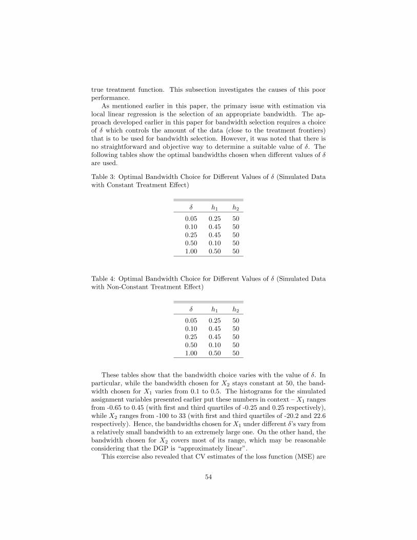
true treatment function. This subsection investigates the causes of this poorperformance.

As mentioned earlier in this paper, the primary issue with estimation vialocal linear regression is the selection of an appropriate bandwidth. The ap-proach developed earlier in this paper for bandwidth selection requires a choiceof δ which controls the amount of the data (close to the treatment frontiers)that is to be used for bandwidth selection. However, it was noted that there isno straightforward and objective way to determine a suitable value of δ. Thefollowing tables show the optimal bandwidths chosen when different values of δare used.

Table 3: Optimal Bandwidth Choice for Different Values of δ (Simulated Datawith Constant Treatment Effect)

δ h1 h2

0.05 0.25 500.10 0.45 500.25 0.45 500.50 0.10 501.00 0.50 50

Table 4: Optimal Bandwidth Choice for Different Values of δ (Simulated Datawith Non-Constant Treatment Effect)

δ h1 h2

0.05 0.25 500.10 0.45 500.25 0.45 500.50 0.10 501.00 0.50 50

These tables show that the bandwidth choice varies with the value of δ. Inparticular, while the bandwidth chosen for X2 stays constant at 50, the band-width chosen for X1 varies from 0.1 to 0.5. The histograms for the simulatedassignment variables presented earlier put these numbers in context – X1 rangesfrom -0.65 to 0.45 (with first and third quartiles of -0.25 and 0.25 respectively),while X2 ranges from -100 to 33 (with first and third quartiles of -20.2 and 22.6respectively). Hence, the bandwidths chosen for X1 under different δ’s vary froma relatively small bandwidth to an extremely large one. On the other hand, thebandwidth chosen for X2 covers most of its range, which may be reasonableconsidering that the DGP is “approximately linear”.

This exercise also revealed that CV estimates of the loss function (MSE) are

54

relatively flat, which was the basis for a criticism leveled against CV methodsby LM (2005), mentioned in the previous section. As an example, for thesimulated dataset with non-constant treatment effect, the MSE estimates (forthe 100 bandwidths considered) from my modified CV procedure with δ = 0.05had a minimum of 0.1341, with first, second and third quartiles of 0.1381, 0.1441and 0.1670 respectively.

Still, this may not be a serious issue if these different bandwidths result insimilar estimates. To determine whether this is the case, regression tables forthe local linear regressions with bandwidths selected using different values of δ,as well as plots of the estimated treatment effect functions are shown below.

The regression tables and plots show that the estimated treatment effectfunctions are fairly similar for bandwidths chosen using different values of δ.This would have been a good sign, if not for the fact that all of these estimatesperform poorly when compared to the true treatment effects underlying theDGPs, especially for the data with non-constant treatment effect.

In particular, the estimated coefficients for the slopes of the estimated treat-ment effect functions (β5 and β6) for the dataset with non-constant treatmenteffect are all negative (although they are statistically insignificant at the 10percent level), in direct contradiction to the true treatment effect, which hasa positive slope. Furthermore, the true treatment effect at the origin in thisdataset, i.e. τ1(0) and τ2(0), given by β1, is zero, but the local linear estimatesfor β1 are all positive and statistically significant at the 5 percent level.

Given that the bandwidth selection procedure considered a relatively com-prehensive grid of potential bandwidth values, it is unlikely that the poor per-formance of the local linear regression method with bandwidth selection viamodified CV was caused by poor implementation alone.

In light of the poor results for MDRD estimation via local linear regres-sion, the rest of this paper focuses on the TPRS estimation method, which hassuperior performance and is far less computationally expensive37.

5.6 Performance of TPRS Estimate when Assignment Vari-ables have Discrete Support

A criticism of the IK bandwidth choice algorithm for local linear regressionin conventional RD is that the algorithm’s asymptotic properties are unknownwhen assignment variables have discrete support. This same argument wasmade against extending the IK bandwidth choice algorithm to MRD in Papayet al. (2011a). Yet, one may also question whether the performance of MRDestimation using TPRS deteriorates when assignment variables have discretesupport. While this paper does not offer theoretical results on this question, Iinvestigate the issue empirically using the simulated datasets.

In fact, the exercise so far already has an assignment variable with discretesupport – GPA, which is reported in hundredths. Yet, there are many possible

37While it may take more than three hours to run the CV bandwidth selection procedurefor local linear regression using δ = 1, a TPRS estimate may be obtained within five seconds.

55

Table 5: Local Linear Regressions Resulting from Different Values of δ (Simu-lated Data with Constant Treatment Effect)

Dependent variable:

College Going

(δ = 0.05) (δ = 0.10) (δ = 0.25) (δ = 0.50) (δ = 1)

β0 0.824∗∗∗ 0.826∗∗∗ 0.826∗∗∗ 0.819∗∗∗ 0.824∗∗∗

(0.005) (0.005) (0.005) (0.006) (0.005)

β1 0.052∗∗ 0.050∗∗ 0.050∗∗ 0.057∗∗∗ 0.052∗∗

(0.022) (0.022) (0.022) (0.022) (0.022)

β2 0.127∗∗∗ 0.144∗∗∗ 0.144∗∗∗ 0.168∗∗∗ 0.138∗∗∗

(0.028) (0.019) (0.019) (0.039) (0.018)

β3 −0.0002 −0.0003 −0.0003 −0.0001 −0.0003(0.0002) (0.0002) (0.0002) (0.0003) (0.0002)

β4 −0.0003 0.001 0.001 0.0004 0.0005(0.001) (0.001) (0.001) (0.002) (0.001)

β5 −0.119 −0.137 −0.137 −0.160∗ −0.130(0.084) (0.084) (0.084) (0.086) (0.084)

β6 −0.001 −0.001 −0.001 −0.001 −0.001(0.001) (0.001) (0.001) (0.001) (0.001)

β7 0.005 0.003 0.003 0.004 0.004(0.004) (0.004) (0.004) (0.004) (0.004)

Obs. 13,581 16,091 16,091 11,282 16,619R2 0.007 0.012 0.012 0.005 0.012

Notes: ∗p<0.1; ∗∗p<0.05; ∗∗∗p<0.01

Treatment effect estimates along the GPA and income frontiers are respectivelygiven by β1 + β6X2 and β1 + β5X1. The treatment coefficients implied by theDGP with constant treatment effect are β1 = 0.025, β5 = 0 and β6 = 0.

56

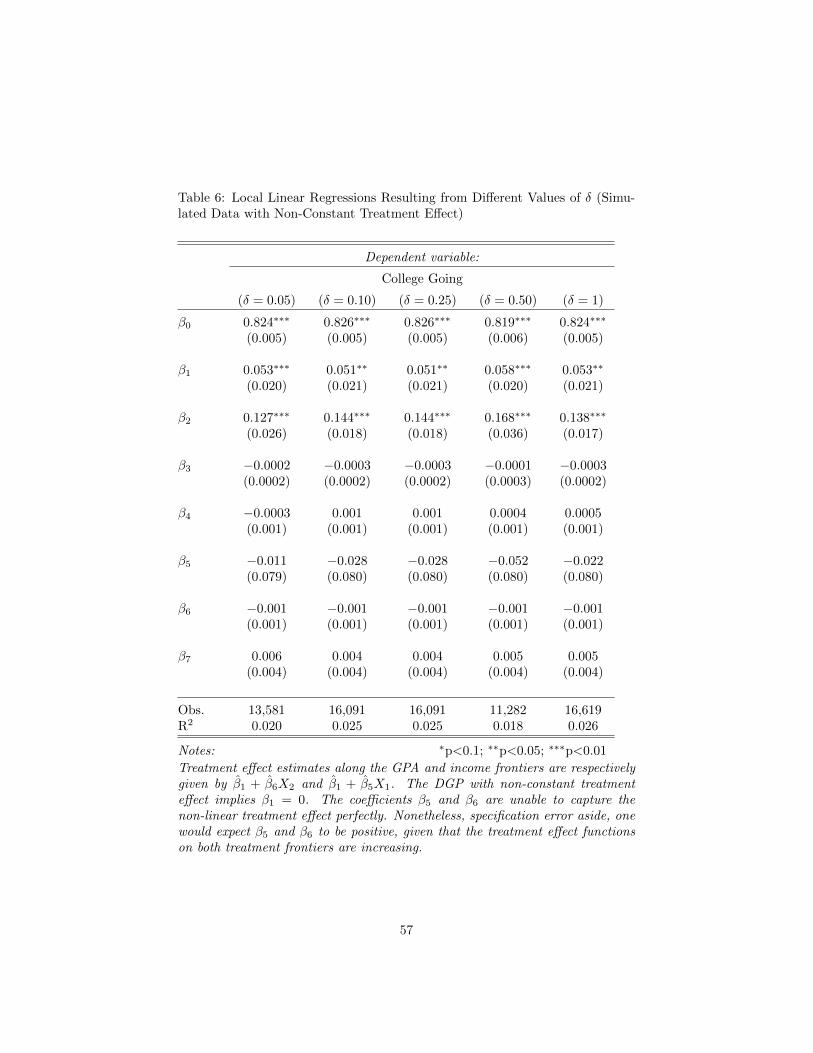
Table 6: Local Linear Regressions Resulting from Different Values of δ (Simu-lated Data with Non-Constant Treatment Effect)

Dependent variable:

College Going

(δ = 0.05) (δ = 0.10) (δ = 0.25) (δ = 0.50) (δ = 1)

β0 0.824∗∗∗ 0.826∗∗∗ 0.826∗∗∗ 0.819∗∗∗ 0.824∗∗∗

(0.005) (0.005) (0.005) (0.006) (0.005)

β1 0.053∗∗∗ 0.051∗∗ 0.051∗∗ 0.058∗∗∗ 0.053∗∗

(0.020) (0.021) (0.021) (0.020) (0.021)

β2 0.127∗∗∗ 0.144∗∗∗ 0.144∗∗∗ 0.168∗∗∗ 0.138∗∗∗

(0.026) (0.018) (0.018) (0.036) (0.017)

β3 −0.0002 −0.0003 −0.0003 −0.0001 −0.0003(0.0002) (0.0002) (0.0002) (0.0003) (0.0002)

β4 −0.0003 0.001 0.001 0.0004 0.0005(0.001) (0.001) (0.001) (0.001) (0.001)

β5 −0.011 −0.028 −0.028 −0.052 −0.022(0.079) (0.080) (0.080) (0.080) (0.080)

β6 −0.001 −0.001 −0.001 −0.001 −0.001(0.001) (0.001) (0.001) (0.001) (0.001)

β7 0.006 0.004 0.004 0.005 0.005(0.004) (0.004) (0.004) (0.004) (0.004)

Obs. 13,581 16,091 16,091 11,282 16,619R2 0.020 0.025 0.025 0.018 0.026

Notes: ∗p<0.1; ∗∗p<0.05; ∗∗∗p<0.01

Treatment effect estimates along the GPA and income frontiers are respectivelygiven by β1 + β6X2 and β1 + β5X1. The DGP with non-constant treatmenteffect implies β1 = 0. The coefficients β5 and β6 are unable to capture thenon-linear treatment effect perfectly. Nonetheless, specification error aside, onewould expect β5 and β6 to be positive, given that the treatment effect functionson both treatment frontiers are increasing.

57

0 5 10 15 20 25 30

0.00

0.01

0.02

0.03

0.04

0.05

Treatment Effect Estimates for Different Values of δGPA Threshold (Constant Treatment Effect)

X2

Trea

tmen

t Effe

ct

True Effectδ=0.05δ=0.10δ=0.25δ=0.50δ=1

0 5 10 15 20 25 30

0.00

0.01

0.02

0.03

0.04

0.05

0.06

Treatment Effect Estimates for Different Values of δGPA Threshold (Non−Constant Treatment Effect)

X2

Trea

tmen

t Effe

ct


Figure 18: Local linear regression estimates of the MDRD treatment effectfunction at the GPA threshold using various values of δ. Note that the red lineis hidden behind the dark green line due to identical bandwidth choice.

58

0.0 0.1 0.2 0.3 0.4

0.00

0.01

0.02

0.03

0.04

0.05

Treatment Effect Estimates for Different Values of δIncome Threshold (Constant Treatment Effect)

X1

Trea

tmen

t Effe

ct


0.0 0.1 0.2 0.3 0.4

0.00

0.01

0.02

0.03

0.04

0.05

0.06

Treatment Effect Estimates for Different Values of δIncome Threshold (Non−Constant Treatment Effect)

X1

Trea

tmen

t Effe

ct


Figure 19: Local linear regression estimates of the MDRD treatment effectfunction at the income threshold using various values of δ. Note that the redline is hidden behind the dark green line due to identical bandwidth choice.

59

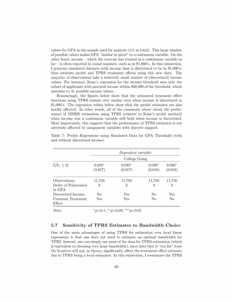
values for GPA in the sample used for analysis (111 in total). This large numberof possible values makes GPA “similar in spirit” to a continuous variable. On theother hand, income – which the exercise has treated as a continuous variable sofar – is often reported in round numbers, such as in $1,000’s. In this subsection,I generate simulated datasets with income that is discretized to be in $1,000’s,then estimate probit and TPRS treatment effects using this new data. Themajority of observations take a relatively small number of (discretized) incomevalues. For instance, Kane’s regression for the income threshold uses only thesubset of applicants with parental income within $20,000 of the threshold, whichamounts to 41 possible income values.

Reassuringly, the figures below show that the estimated treatment effectfunctions using TPRS remain very similar even when income is discretized in$1,000’s. The regression tables below show that the probit estimates are alsohardly affected. In other words, all of the comments above about the perfor-mance of MDRD estimation using TPRS (relative to Kane’s probit method)when income was a continuous variable still hold when income is discretized.Most importantly, this suggests that the performance of TPRS estimates is notadversely affected by assignment variables with discrete support.

Table 7: Probit Regressions using Simulated Data for GPA Threshold (withand without discretized income)

Dependent variable:

College Going

I[X1 ≥ 0] 0.033∗ 0.033∗ 0.030∗ 0.030∗

(0.017) (0.017) (0.016) (0.016)

Observations 11,750 11,750 11,750 11,750Order of Polynomial 3 3 3 3in GPADiscretized Income No Yes No YesConstant Treatment Yes Yes No NoEffect

Note: ∗p<0.1; ∗∗p<0.05; ∗∗∗p<0.01

5.7 Sensitivity of TPRS Estimates to Bandwidth Choice

One of the main advantages of using TPRS for estimation over local linearregressions is that one does not need to estimate an optimal bandwidth forTPRS. Instead, one can simply use most of the data for TPRS estimation (whichis equivalent to choosing very large bandwidth), since data that is “too far” fromthe frontiers will not, in theory, significantly affect the treatment effect estimatedue to TPRS being a local estimator. In this subsection, I reestimate the TPRS

60

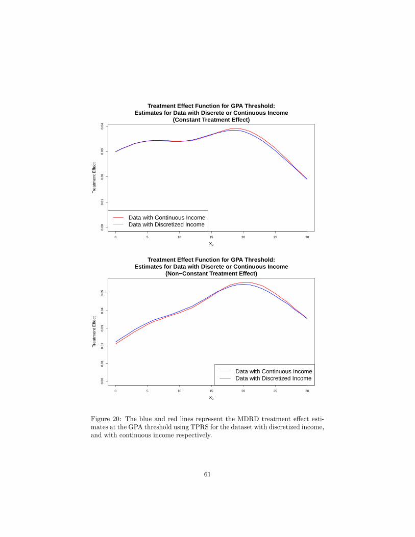
0 5 10 15 20 25 30

0.00

0.01

0.02

0.03

0.04

Treatment Effect Function for GPA Threshold:Estimates for Data with Discrete or Continuous Income

(Constant Treatment Effect)

X2

Trea

tmen

t Effe

ct

Data with Continuous IncomeData with Discretized Income

0 5 10 15 20 25 30

0.00

0.01

0.02

0.03

0.04

0.05

Treatment Effect Function for GPA Threshold:Estimates for Data with Discrete or Continuous Income

(Non−Constant Treatment Effect)

X2

Trea

tmen

t Effe

ct


Figure 20: The blue and red lines represent the MDRD treatment effect esti-mates at the GPA threshold using TPRS for the dataset with discretized income,and with continuous income respectively.

61

0.0 0.1 0.2 0.3 0.4

0.00

00.

005

0.01

00.

015

0.02

00.

025

0.03

0

Treatment Effect Function for Income Threshold:Estimates for Data with Discrete or Continuous Income

(Constant Treatment Effect)

X1

Trea

tmen

t Effe

ct


0.0 0.1 0.2 0.3 0.4

0.00

0.01

0.02

0.03

0.04

0.05

0.06

Treatment Effect Function for Income Threshold:Estimates for Data with Discrete or Continuous Income

(Non−Constant Treatment Effect)

X1

Trea

tmen

t Effe

ct


Figure 21: The blue and red lines represent the MDRD treatment effect es-timates at the income threshold using TPRS for the dataset with discretizedincome, and with continuous income respectively.

62

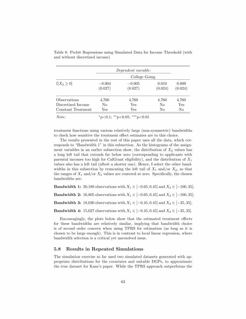
Table 8: Probit Regressions using Simulated Data for Income Threshold (withand without discretized income)

Dependent variable:

College Going

I[X2 ≥ 0] −0.004 −0.005 0.010 0.009(0.027) (0.027) (0.024) (0.024)

Observations 4,760 4,760 4,760 4,760Discretized Income No Yes No YesConstant Treatment Yes Yes No No

Note: ∗p<0.1; ∗∗p<0.05; ∗∗∗p<0.01

treatment functions using various relatively large (non-symmetric) bandwidthsto check how sensitive the treatment effect estimates are to this choice.

The results presented in the rest of this paper uses all the data, which cor-responds to “Bandwidth 1” in this subsection. As the histograms of the assign-ment variables in an earlier subsection show, the distribution of X2 values hasa long left tail that extends far below zero (corresponding to applicants withparental incomes too high for CalGrant eligibility), and the distribution of X1

values also has a left tail (albeit a shorter one). Hence, I select the other band-widths in this subsection by truncating the left tail of X1 and/or X2, so thatthe ranges of X1 and/or X2 values are centered at zero. Specifically, the chosenbandwidths are:

Bandwidth 1: 20,180 observations withX1 ∈ [−0.65, 0.45] andX2 ∈ [−100, 35];



Bandwidth 4: 15,027 observations withX1 ∈ [−0.45, 0.45] andX2 ∈ [−35, 35].

Encouragingly, the plots below show that the estimated treatment effectsfor these bandwidths are relatively similar, implying that bandwidth choiceis of second order concern when using TPRS for estimation (as long as it ischosen to be large enough). This is in contrast to local linear regression, wherebandwidth selection is a critical yet unresolved issue.

5.8 Results in Repeated Simulations

The simulation exercise so far used two simulated datasets generated with ap-propriate distributions for the covariates and suitable DGPs, to approximatethe true dataset for Kane’s paper. While the TPRS approach outperforms the

63

0.000

0.025

0.050

0 10 20 30

X2

Tre

atm

en

t E

ffe

ct

Bandwidth 1Bandwidth 2Bandwidth 3Bandwidth 4

Treatment Effect Estimates for GPA Threshold(Constant Treatment Effect)

0.000

0.025

0.050

0 10 20 30

X2

Tre

atm

en

t E

ffe

ct


Treatment Effect Estimates for GPA Threshold(Non−Constant Treatment Effect)

Figure 22: TPRS estimates of the treatment effect function at the GPA thresh-old are plotted for various choices of bandwidth. The true effect is shown inblack.

64

0.000

0.025

0.050

0.0 0.1 0.2 0.3 0.4

X1

Tre

atm

en

t E

ffe

ct


Treatment Effect Estimates for Income Threshold(Constant Treatment Effect)

0.000

0.025

0.050

0.0 0.1 0.2 0.3 0.4

X1

Tre

atm

en

t E

ffe

ct


Treatment Effect Estimates for Income Threshold(Non−Constant Treatment Effect)

Figure 23: TPRS estimates of the treatment effect function at the income thresh-old are plotted for various choices of bandwidth. The true effect is shown inblack.

65

probit regression on these simulated datasets, it is possible that the TPRS esti-mate just happened to perform well on these particular realizations of the data.In this subsection, I assess the performance of the TPRS estimation approach byrepeatedly generating datasets (a total of 1,000 times) using the same covariatedistributions and DGPs as before, and obtaining TPRS and probit estimatesfor each realization of the data.38

5.8.1 Mean Squared Integrated Error of the TPRS and Probit Es-timates

A metric is needed to compare the TPRS and probit estimates of the treatmentfunction. MSE is a common measure for comparing the accuracies of scalarestimators when the true parameter value is known. However, the estimatein this case is a function rather than a scalar. Hence, rather than reportingthe MSEs for a grid of points, I report the Mean Integrated Squared Error(MISE), which provides a more convenient summary of the global accuracy ofthe function estimate. In this example, given the true treatment function τ1 (orτ2) and its estimate τ1 (or τ2), the MISE is defined by:39

(21) MISE(τk, τk) ≡∫Fk

(τk − τk)2dxk′ , where k ∪ k′

= {1, 2}.

The following table shows that on average the TPRS estimate far outper-forms the probit estimate in terms of MISE. The four cases considered cor-respond to the estimates for the two different DGPs (constant/non-constanttreatment effect) along the two frontiers (GPA and income). In all four cases,the MISE for the TPRS estimate is smaller than that for the probit estimate(in fact, the TPRS MISE is 2.4 to 3.3 times smaller along the income frontier).

5.8.2 Performance of the TPRS Bayesian Confidence Intervals

In addition to comparing the accuracies of the TPRS and probit estimates, therepeated simulations also allow me to assess the performance of the conservativeBayesian confidence intervals. One may recall from the previous section thatprovided the error term has a normal distribution, the coefficient estimates forthe basis functions of the TPRS (and hence, the point estimates of the treatmenteffect) are normally distributed. However, this simulation exercise is based on

38I did not perform this exercise for the local linear estimate due to the computationalexpense of the bandwidth selection procedure. For instance, selecting a bandwidth usingδ = 1 takes more than three hours, which makes repeating the procedure 1,000 times on asingle machine intractable.

39For computational reasons, I approximate this integral using the value of the integrandat the left endpoint for a grid of values along the frontier (31 values from 0 to 30 for F1 and41 values from 0 to 0.40 for F2). While this integral approximation is rather crude, it wouldnot be badly biased unless the integrand is systematically increasing or decreasing over therange of the frontier (which does not appear to be the case). Moreover, the focus here is onthe difference in MISE between the TPRS and probit estimators, rather than the exact valueof the MISE. It turns out that the difference between the MISE of these two estimators islarge enough to alleviate such concerns.

66

Table 9: Comparison of MISE’s for TPRS and Probit Estimates

Treatment Frontier TPRS MISE Probit MISE Ratio of MISE’s(Probit/TPRS)

Constant GPA 0.006 0.009 1.421Non-Constant GPA 0.009 0.010 1.106

Constant Income 0.0001 0.0003 2.431Non-Constant Income 0.0001 0.0005 3.262

a probability model where the dichotomous outcome variable can only take thevalues of zero or one, which implies that the assumption of normally distributederror terms is violated. Hence, normality of the treatment point estimates isonly an approximation based on large sample theory. The large number of TPRSestimates and their Bayesian CIs will shed light on whether this approximationis a valid one.

There are two questions to answer concerning the distributions of the pointestimates. The first and arguably more important concern is whether theBayesian 95 percent CIs cover the true function value at least 95 percent ofthe time. The second is whether the distributions of the point estimates areapproximately normal.

The following plots show the coverage rates for the TPRS and probit CIs inthe 1,000 simulations under the two DGPs (as before, the conservative BayesianCIs are used for TPRS). For the simulated data with constant treatment effect,the TPRS CIs have very high coverage rates (about 98 to 99 percent) alongthe entire ranges of both frontiers. The TPRS CIs tend to have lower coveragerates near the origin for the simulated data with non-constant treatment effect,although moving away from the origin, the coverage rates are typically at least95 percent. Regardless of the frontier or the dataset in question, the TPRS CIstend to have higher coverage rates on average than the probit CIs.

To address the second concern, histograms of several point estimates areshown below. These empirical distributions seem approximately normal, inthat they are unimodal and are not systematically skewed in either direction.

5.8.3 Shape of the TPRS Treatment Effect Estimate

The final issue explored in this subsection concerns whether the shape of theaverage TPRS function estimate is similar to that of the true treatment function.To this end, I plot the means of the TPRS point estimates along a grid ofpoints on each frontier (for both the DGPs with constant and non-constanttreatments). I also overlay the true treatment functions in these graphs forcomparison.

The graphs below show that the TPRS estimates at the income thresholdtend to approximate the shape of the true function quite well, while TPRS es-timates at the GPA frontier show some sinusoidal behavior. This is an artifact

67

● ●

●●

●

● ●

● ●●

●

●●

● ●●

●

●

●

●● ●

●●

●● ●

● ●

●

●

0.900

0.925

0.950

0.975

1.000

0 10 20 30

X2

Cov

erag

e P

roba

bilit

y

● TPRS (Constant Treatment)

TPRS (Non−Constant Treatment)

Probit (Constant Treatment)

Probit (Non−Constant Treatment)

Coverage Probabilities forEstimates at GPA Threshold

Figure 24: The various lines show the empirical coverage over 1,000 simulationsof the two estimators using the two different simulated datasets for differentvalues of X2 along the GPA frontier. The black line shows the 95 percentcoverage level.

68

●● ● ● ● ●

● ●● ● ● ● ●

● ●● ● ●

● ● ●● ● ● ● ● ●

● ● ● ● ● ● ● ● ●● ● ●

● ●

0.900

0.925

0.950

0.975

1.000

0.0 0.1 0.2 0.3 0.4

X1

Cov

erag

e P

roba

bilit

y

● TPRS (Constant Treatment)

TPRS (Non−Constant Treatment)

Probit (Constant Treatment)

Probit (Non−Constant Treatment)

Coverage Probabilities forEstimates at Income Threshold

Figure 25: The various lines show the empirical coverage over 1,000 simulationsof the two estimators using the two different simulated datasets for differentvalues of X1 along the income frontier. The black line shows the 95 percentcoverage level.

69

X2 = 0

Fre

quen

cy

050

100

150

200

250

X2 = 10

Fre

quen

cy

050

100

150

200

250

X2 = 20

Fre

quen

cy

050

100

150

200

250

300

X2 = 30

Fre

quen

cy

050

100

150

200

250

Figure 26: Distribution of TPRS point estimates along the GPA frontier for thesimulated dataset with constant treatment effect.

X1 = 0

Fre

quen

cy

050

100

150

200

250

X1 = 0.1

Fre

quen

cy

050

100

150

200

250

X1 = 0.2

Fre

quen

cy

050

100

150

200

250

X1 = 0.3

Fre

quen

cy

050

100

150

200

250

X1 = 0.4

Fre

quen

cy

050

100

150

200

250

Figure 27: Distribution of TPRS point estimates along the income frontier forthe simulated dataset with constant treatment effect.

X2 = 0

Fre

quen

cy

050

100

150

200

X2 = 10

Fre

quen

cy

050

100

150

200

250

300

X2 = 20

Fre

quen

cy

050

100

150

200

250

300

X2 = 30

Fre

quen

cy

050

100

150

200

250

Figure 28: Distribution of TPRS point estimates along the GPA frontier for thesimulated dataset with non-constant treatment effect.

70

X1 = 0F

requ

ency

050

100

150

200

X1 = 0.1

Fre

quen

cy

050

100

150

200

250

X1 = 0.2

Fre

quen

cy

050

100

150

200

250

X1 = 0.3

Fre

quen

cy

050

100

150

200

250

X1 = 0.4

Fre

quen

cy

050

100

150

200

250

Figure 29: Distribution of TPRS point estimates along the income frontier forthe simulated dataset with non-constant treatment effect.

of the periodic behavior in the true DGPs along the GPA frontier that is im-perfectly captured by the TPRS estimates (as mentioned several times earlier).Nonetheless, if one abstracts from this oscillation about the trend, the generalshape of the TPRS estimate at the GPA threshold is also similar to that of thetrue function.

6 Additional Considerations

6.1 Fuzzy MRD

Thus far, this paper has only considered sharp MRD, where treatment is com-pletely determined by values of the assignment variables. Here, I discuss fuzzyMRD and describe how the treatment effect function may be estimated, startingwith the case for dichotomous treatment. I abbreviate fuzzy MRD in generalas FMRD, with the dichotomous and multiple treatment cases respectively ab-breviated as FMDRD and FMMRD.

6.1.1 FMDRD

Similar to conventional fuzzy RD, FMRD refers to situations where the jumpin probability of receiving treatment when crossing a threshold is less than one.However, instead of a scalar threshold as in conventional RD, there are severalone-dimensional frontiers in FMRD. Complicating matters further, it is possiblefor the FMRD on one frontier to be fuzzy even when the FMRD on anotherfrontier is sharp, or for the jump in treatment probability to be one on part ofa frontier and less than one on the rest of the same frontier. The following twoexamples show how such situations may arise in reality.

To illustrate how the jump in probability may vary along a single frontier,consider a state financial aid package where eligibility depends, without ex-ceptions, on high school students having GPA and family income respectivelyabove and below their thresholds. However, not all eligible applicants apply.Assuming the sample is the entire population of high school students (rather

71

●●

●

●

● ●

●

●●

●

●●

●

●

●●

●

●●

●

● ●

●

● ●

●

●●

●

●

●

0.00

0.01

0.02

0.03

0 10 20 30

X2

Est

imat

ed T

reat

men

t Effe

ct

● Mean TPRS EstimateTrue Effect

Mean Estimated Treatment Effects(GPA Frontier, Constant Treatment Effect)

●● ●

●●

●

●

●

● ●● ●

●

●

● ●

●●

●

●

●●

●●

●

●

●

●

●

●●

0.00

0.01

0.02

0.03

0.04

0 10 20 30

X2

Est

imat

ed T

reat

men

t Effe

ct


Mean Estimated Treatment Effects(GPA Frontier, Non−Constant Treatment Effect)

Figure 30: Mean TPRS estimates at the GPA threshold are shown in blue. Theblack line represents the true treatment effect.

72

● ● ● ● ● ● ● ● ● ● ● ● ● ● ● ● ● ● ● ● ● ● ● ● ● ● ● ● ● ● ● ● ● ● ● ● ● ● ● ● ●

0.00

0.01

0.02

0.03

0.0 0.1 0.2 0.3 0.4

X1

Est

imat

ed T

reat

men

t Effe

ct


Mean Estimated Treatment Effects(Income Frontier, Constant Treatment Effect)

●●

●●

●●

●●

●●

●●

●●

●●

●●

●●

●●

●●

●●

●●

●●

●●

●●

●●

●●

●●

●

0.00

0.02

0.04

0.06

0.0 0.1 0.2 0.3 0.4

X1

Est

imat

ed T

reat

men

t Effe

ct


Mean Estimated Treatment Effects(Income Frontier, Non−Constant Treatment Effect)

Figure 31: Mean TPRS estimates at the income threshold are shown in blue.The black line represents the true treatment effect.

73

than just the applicants), and using whether one receives the aid package asthe treatment variable, this becomes a FMDRD problem. Now, the decisionof eligible applicants to apply (or not) may vary depending on his/her familyincome. It is quite plausible that for students with family incomes far belowthe income threshold, the aid package is extremely attractive, so that the jumpin probability at the GPA threshold is one for low values of income. On theother hand, students with family income just below the income threshold maybe less influenced by the aid package, so the jump in probability at the GPAthreshold is less than one for higher values of income (that are still below theincome threshold).

This next example has the same basic setup, with eligibility for a finan-cial aid package depending on GPA and family income. Now, suppose thatthe family income threshold is very low and that the aid package can only beused for public colleges. Assume further that all eligible students who barelypass the GPA threshold apply, since the aid package is extremely attractive forthese students from very poor families (by definition of being below the incomethreshold). Hence, the jump in treatment probability at the GPA threshold isone. On the other hand, suppose that among the eligible students just belowthe income threshold, some of the students with high GPAs (far above the GPAthreshold) do not apply because of scholarship offers they receive from privatecolleges. This constitutes a case where the MDRD on one frontier (i.e. theGPA threshold) is sharp, whereas the MDRD on another frontier (specifically,the income threshold) is fuzzy.

In practice, one can get a sense of whether the FMRD is fuzzy along afrontier by examining discontinuity plots created using the “slicing” approach(described in section 3.1) with probability of receiving treatment on the verticalaxis.

Having discussed the basic concepts of FMDRD, I now define it more for-mally. The following definition pertains to a FMDRD for the frontier F1 (thedefinition of FMDRD for F2 is completely analogous). Assume that

limx1→0+

E[Wi|X1i = x1, X2i = x2]− limx1→0−

E[Wi|X1i = x1, X2i = x2] < 1

for some x2 ≥ 0, and

limx1→0+

E[Wi|X1i = x1, X2i = x2] 6= limx1→0−

E[Wi|X1i = x1, X2i = x2]

for all x2 ≥ 0.40 Then, denoting

f(x1, x2) ≡ E[Y |X1i = x1, X2i = x2],

p(x1, x2) ≡ E[W |X1i = x1, X2i = x2],

40One may relax this assumption by requiring it only for a subset of F1. However, shouldone choose to do so, care must be taken in choosing the domain of definition for the treatmentfunction estimate to avoid division by zero.

74

the FMDRD treatment effect function along F1 is defined as:

(22) τFuzzy1 (x2) ≡ limx1→0+ f(x1, x2)− limx1→0− f(x1, x2)

limx1→0+ p(x1, x2)− limx1→0− p(x1, x2)for x2 ≥ 0.

TPRS estimates for the numerator and denominator can be obtained usingthe approach outlined in section 4.3 (with ultimate outcome Y and treatmentstatus W as the outcome variables respectively).

To elaborate, I denote the TPRS fitted using observations in the non-negativequadrant R1 with Y and W as the outcome variables respectively by f1(x1, x2)

and p1(x1, x2), and those fitted on R2 \ R1 by f0(x1, x2) and p0(x1, x2). Thisallows the point estimate of the treatment effect at any point along the frontierF1 to be written as:

(23) τFuzzy1 (x2) ≡ f1(0, x2)− f0(0, x2)

p1(0, x2)− p0(0, x2)for x2 ≥ 0.

The point estimates for the numerator and denominator of the FMDRDtreatment functions have posterior Bayesian distributions that are (approxi-mately) normal, as explained at the end of section 4. However, it is unlikelythat a useful theoretical approximation for the distribution of the FMDRD pointestimate can be found without knowing the exact distributions of the numera-tor and denominator as well as their correlation. In particular, ratios of normalrandom variables need not be well behaved.41

Hence, rather than deriving theoretical CIs for the FMDRD estimate, a morepractical approach may be to obtain CIs by bootstrapping. Unless the dataset ishuge, the computational burden is unlikely to be excessive – computing a MDRDestimate for the simulated dataset in the previous section (which contains almost20,000 observations) takes less than five seconds on a personal laptop. Thisflexibility is the main reason TPRS is preferred over thin plate splines, sincebootstrapping with the latter would not be feasible even with moderately largedatasets due to its computational expense.

If the FMDRD is fuzzy on both frontiers, one can simply use the formulaabove to obtain τFuzzy1 (x2), and compute τFuzzy2 (x1) similarly using the for-mula:

(24) τFuzzy2 (x1) ≡ f1(x1, 0)− f0(x1, 0)

p1(x1, 0)− p0(x1, 0)for x1 ≥ 0.

Point-wise CIs can then be obtained via bootstrap for both functions.However, there is a choice to be made when the FMDRD is fuzzy on one

frontier (say F1) but sharp on the other (F2 in this case). τFuzzy1 (x2) should ofcourse be estimated using the FMDRD formula as before, with point-wise CIsobtained by bootstrapping. On the other hand, one can either use τFuzzy2 (x1)

41For instance, the ratio of two independent standard normal random variables follows aCauchy distribution, which has undefined mean and variance.

75

for estimation of the treatment effect function along F2, or τSharp2 (x1), which isdefined by:

(25) τSharp2 (x1) ≡ f1(x1, 0)− f0(x1, 0) for x1 ≥ 0.

The advantages of using τSharp2 (x1) are that this estimator has lower biasif the FMDRD is truly sharp on the frontier F2, and Bayesian CIs can beused. However, it will be the case that in general, τSharp2 (0) 6= τFuzzy1 (0) as

long as f1(0, 0) − f0(0, 0) 6= 0 and p1(0, 0) − p0(0, 0) 6= 1. By contrast, using

the fuzzy treatment effect estimates for both frontiers ensures that τFuzzy2 (0) =

τFuzzy1 (0). Moreover, obtaining bootstrapped CIs for τFuzzy2 (x1) imposes almostno additional computational burden, since bootstrapping is already done forτFuzzy1 (x2).42

6.1.2 FMMRD

Next, I show that with the exception of a slight complication, the procedurefor estimating FMMRD is essentially the same. Suppose that there are fourtreatments conditions, roughly corresponding to each of the four quadrants ofR2, and consider for this example, estimation of the treatment function τ12(x2)along F12, the non-negative x2-axis.

Most of the observations in Rk (k = 1, 2, 3, 4) consists of observations withtreatment k (i.e. satisfy Wki = 1). However, there may be observations inR1 ∪ R2 that satisfy neither W1i = 1 nor W2i = 1. For this example, supposefor concreteness that there are observations in R2 that receive treatment 3.43

Estimation of τ12(x2), which compares treatment 1 to treatment 2, may beinvalidated by observations that receive neither treatment. Therefore, only ob-servations receiving treatments 1 or 2 should be used in estimating the treatmenteffect τ12(x2). After discarding observations in R1 ∪ R2 with neither W1i = 1nor W2i = 1, one may then use graphical analysis to decide whether to estimateτSharp12 (x2) or τFuzzy12 (x2). Also, notice that in this example, the presence ofobservations receiving treatment 3 in R2 suggests that the MMRD along thefrontier F23 may be a fuzzy one.

6.2 Inclusion of Baseline Covariates

In this subsection, the vector of assignment variables is denoted by X and thevector of baseline covariates by Z. If the MRD assumptions are valid, one wouldexpect the density of Z conditional on X, fZ|X(z|x), to be continuous at the

42To see this, note that during each bootstrap replication b to obtain the bootstrap estimate

τFuzzy1b (x2) of τ1(x2), the functions f1b, f0b, p1b and p0b are fitted. Therefore, the only

additional calculation required to obtain a bootstrap estimate τFuzzy2b (x1) of τ2(x1) is simply

to compute the formula for τFuzzy2b (x1) using the functions f1b, f0b, p1b and p0b, which have

already been fit.43This situation can only arise in FMMRD, since observations in FMDRD can only be in

the treatment or control group by definition.

76

frontiers44. Assuming this holds, it follows that for X arbitrarily close to afrontier, the baseline covariates Z are independent of the treatment W . Takingthe frontier F1 in a MDRD as an example, this implies that for x2 ≥ 0,

limx1→0+

E[Y |X1i = x1, X2i = x2,Z = z]

− limx1→0−

E[Y |X1i = x1, X2i = x2,Z = z]

= limx1→0+

E[Y |X1i = x1, X2i = x2]− limx1→0−

E[Y |X1i = x1, X2i = x2].

So, provided the MRD assumptions hold, the inclusion of additional co-variates in the estimation equation for MRD should not change the estimatedfunction by much. Testing the sensitivity of MRD estimates to the inclusion ofbaseline covariates can thus be used as an additional check on the validity ofthe MRD design.

A useful feature of TPRS is that it can easily be incorporated into generalizedadditive models. This provides a great deal of flexibility for how a user may wishto include the baseline covariates in the model. For example, one can estimate

Yi = g1(Xi) + g2(Zi) + εi,

where g1 is the TPRS described in section 4, and g2 is a linear function of thebaseline covariates, or

Yi = g(Xi,Zi) + εi,

where g is a TPRS in X and Z, just to list two possibilities.Another alternative, motivated by the discussion in Lee and Lemieux (2010),

is to “residualize” the outcome variable Y . Specifically, one first fits a modelwith Y as a function of Z, then conducts MRD estimation using the residualsfrom the first model as the outcome variable.

6.3 More than Two Assignment Variables

Although most of the discussion in this paper has focused on MRD with twoassignment variables, the estimation methods described still work in theoryfor more than two assignment variables, provided appropriate adjustments aremade. First, with d assignment variables, the treatment frontiers are (d − 1)-dimensional surfaces. Hence, the estimated treatment effect for a given frontieris typically a function of d − 1 assignment variables. Second, the smoothnesspenalty term Jmd that is used for fitting TPRS surfaces should satisfy 2m >d+ 1.

However, estimation in higher-dimensional assignment variable space is notwithout difficulties. Perhaps the most important of these is sparsity of data

44In fact, the diagnostic graphs that plot predetermined outcomes as functions of the as-signment variables (discussed in section 3.2) are designed to check whether this conditionholds.

77

resulting from the curse of dimensionality. The following toy example illustratesthis point.

Consider a MDRD with d assignment variables, and assume that values ofthe assignment variables in the data is uniformly distributed in a d-dimensionalunit hypercube, with the cutoffs for each assignment variable at 0.5. Typically,only data that is “close” to the boundary is truly relevant for MRD estimation45,which I assume to be data that is at most a distance of b from the boundary.Using the distance function induced by the L∞-norm (i.e. the max-norm) to begenerous46, the total fraction of data that is relevant in this toy example is givenby (0.5+b)d− (0.5−b)d. The fraction of data that is relevant for estimating thetreatment function along each frontier is approximately this quantity divided byd, since there are d treatment frontiers in the d-dimensional assignment variablespace. The following table shows that the proportion of data that is relevantfor estimation decreases rapidly as the dimension d grows (using b = 0.1)47.

Table 10: Toy Example of Curse of Dimensionality

d Proportion of Data Relevant Proportion of Data Relevantfor Each Frontier

2 0.200 0.1003 0.152 0.0514 0.104 0.0265 0.068 0.0146 0.043 0.0077 0.026 0.0048 0.016 0.0029 0.010 0.00110 0.006 0.001

This suggests that when possible, one should try to reduce the dimensionof the assignment variable space, especially when several assignment variablesrepresent different measures of the “same” underlying characteristic (in a qual-itative sense).

To elaborate, consider an example where eligibility for a college financial aidpackage depends on family income being below a threshold, and the test score

45One should not confuse this point with the fact that TPRS estimation can be done usingnearly all the data. In particular, TPRS is a local estimator, so that data far from theboundary has limited effect on estimates at the boundary. Hence, the decision to use mostof the data for TPRS estimation is simply to avoid the tedious and tricky task of optimalbandwidth selection, rather than in the hope that data far from the boundary can improveestimates at the boundary.

46Using any other distance function induced by Lp-norms for p < ∞ will lead to less databeing considered relevant for treatment effect estimation.

47For MMRD, a greater proportion of the data is closer to at least one frontier. However,the number of frontiers separating the multiple treatment conditions is also greater, so theproblem is no less serious.

78

on each of the three SAT components (reading, writing and language, and math)being at least 600. It would be easy to set this up as a four-dimensional MDRDproblem, but this is undesirable due to the curse of dimensionality (which willlead to imprecise estimates due to the sparsity of data close to each frontierin the four-dimensional space). Instead, one can collapse the three SAT scores(X2, X3, X4) into a single assignment variable X2 defined by

X2 = min{X2 − 600, X3 − 600, X4 − 600},

since they all represent academic performance. In particular, one is unlikelyto gain useful insights by distinguishing between say, the effect of crossing thereading score threshold versus the effect of crossing the writing and languagescore threshold. So in this context, essentially no information is lost using thisdimension reduction method, and the resulting treatment effect estimate is alsolikely to be more precise, since a greater proportion of data will be close to thetreatment boundaries in the new two-dimensional assignment variable space.

However, one would need to make sure that the variables are scaled similarlywhen using this approach. While this is not a problem for the SAT scores,the inclusion of a GPA requirement will necessitate rescaling of variables beforeusing this dimension-reduction technique, since GPA will almost always be closerto its cutoff than the SAT scores are from theirs.

6.4 Uncertainty over the Number of Treatments

Sometimes, it is not clear exactly what constitutes a treatment condition for aparticular MRD. For example, suppose the two assignment variables are readingand math scores which determine whether a student is required to take summerremediation classes for reading and/or math (depending on the respective testscores). Defining the treatment as whether or not a student attends any summerremediation results in a MDRD design, whereas distinguishing between types ofsummer remediation leads to a MMRD design.

A practical way to deal with uncertainty over treatment definition is to firstestimate a MMRD (which defines a greater number of treatment conditions)and check whether the point-wise CIs for estimated treatment effects along eachfrontier typically contains zero. In the context of the example above, one mayexamine the estimated treatment functions for the frontiers separating studentswho failed one test, and students who failed both tests. If these estimatedtreatment functions tend not to be significantly different from zero, then onemay consider reformulating the problem as a MDRD.

7 Conclusion

While MRD is a useful tool for a wide range of policy evaluations, the currentliterature on this research design is limited. As such, there is little by way ofconsensus on how to conduct analysis for MRD. This paper discusses the existingresearch on MRD, and propose novel methods that address their shortcomings.

79

In particular, this paper contains the first extensive discussion of graphicalmethods for MRD. Graphical analysis is a critical component of conventionalRD, but has been largely neglected in the MRD literature thus far. I dis-cuss the advantages of estimating flexible treatment effect functions over scalartreatment effects, and provide numerous examples where the former may yieldvaluable insights. This paper also generalizes an existing method for estimatingtreatment effect functions using local linear regression, and proposes a separatenew method using thin plate regression splines (TPRS) that is easy to imple-ment. Finally, through a simulation study based closely on real data, I showthat the estimation approach using TPRS consistently outperforms existing es-timation methods on the simulated data.

The simulation results suggest that MRD treatment function estimation us-ing TPRS holds promise. Here, I suggest two related issues that merit furtherinvestigation. First, the theoretical properties of the TPRS estimation methodhave not been developed in depth. For instance, this paper does not provideformal results on its asymptotic convergence properties. Second, a compari-son between MRD treatment effect functions estimated on a real dataset usingTPRS and local linear regression (with bandwidth chosen either via my gener-alization of LM CV or a multidimensional analogue of the IK algorithm) mayyield additional insights.

80

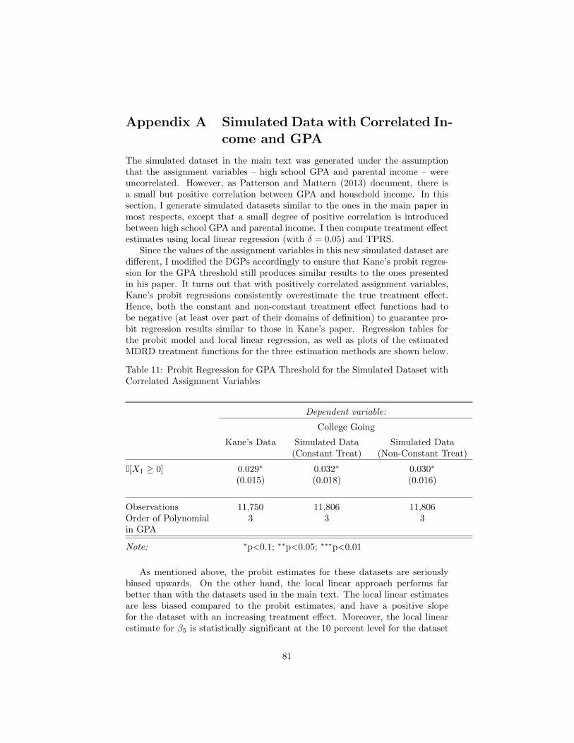
Appendix A Simulated Data with Correlated In-come and GPA

The simulated dataset in the main text was generated under the assumptionthat the assignment variables – high school GPA and parental income – wereuncorrelated. However, as Patterson and Mattern (2013) document, there isa small but positive correlation between GPA and household income. In thissection, I generate simulated datasets similar to the ones in the main paper inmost respects, except that a small degree of positive correlation is introducedbetween high school GPA and parental income. I then compute treatment effectestimates using local linear regression (with δ = 0.05) and TPRS.

Since the values of the assignment variables in this new simulated dataset aredifferent, I modified the DGPs accordingly to ensure that Kane’s probit regres-sion for the GPA threshold still produces similar results to the ones presentedin his paper. It turns out that with positively correlated assignment variables,Kane’s probit regressions consistently overestimate the true treatment effect.Hence, both the constant and non-constant treatment effect functions had tobe negative (at least over part of their domains of definition) to guarantee pro-bit regression results similar to those in Kane’s paper. Regression tables forthe probit model and local linear regression, as well as plots of the estimatedMDRD treatment functions for the three estimation methods are shown below.

Table 11: Probit Regression for GPA Threshold for the Simulated Dataset withCorrelated Assignment Variables

Dependent variable:

College Going


I[X1 ≥ 0] 0.029∗ 0.032∗ 0.030∗

(0.015) (0.018) (0.016)

Observations 11,750 11,806 11,806Order of Polynomial 3 3 3in GPA

Note: ∗p<0.1; ∗∗p<0.05; ∗∗∗p<0.01

As mentioned above, the probit estimates for these datasets are seriouslybiased upwards. On the other hand, the local linear approach performs farbetter than with the datasets used in the main text. The local linear estimatesare less biased compared to the probit estimates, and have a positive slopefor the dataset with an increasing treatment effect. Moreover, the local linearestimate for β5 is statistically significant at the 10 percent level for the dataset

81

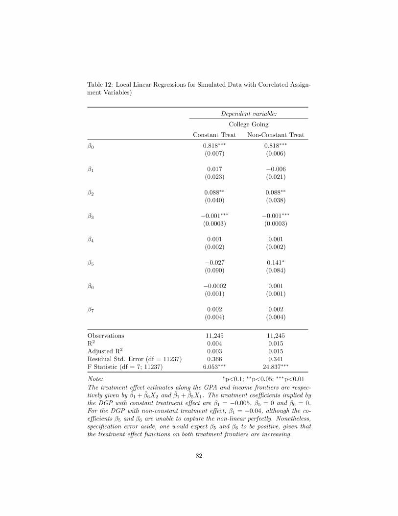
Table 12: Local Linear Regressions for Simulated Data with Correlated Assign-ment Variables)

Dependent variable:

College Going

Constant Treat Non-Constant Treat

β0 0.818∗∗∗ 0.818∗∗∗

(0.007) (0.006)

β1 0.017 −0.006(0.023) (0.021)

β2 0.088∗∗ 0.088∗∗

(0.040) (0.038)

β3 −0.001∗∗∗ −0.001∗∗∗

(0.0003) (0.0003)

β4 0.001 0.001(0.002) (0.002)

β5 −0.027 0.141∗

(0.090) (0.084)

β6 −0.0002 0.001(0.001) (0.001)

β7 0.002 0.002(0.004) (0.004)

Observations 11,245 11,245R2 0.004 0.015Adjusted R2 0.003 0.015Residual Std. Error (df = 11237) 0.366 0.341F Statistic (df = 7; 11237) 6.053∗∗∗ 24.837∗∗∗

Note: ∗p<0.1; ∗∗p<0.05; ∗∗∗p<0.01

The treatment effect estimates along the GPA and income frontiers are respec-tively given by β1 + β6X2 and β1 + β5X1. The treatment coefficients implied bythe DGP with constant treatment effect are β1 = −0.005, β5 = 0 and β6 = 0.For the DGP with non-constant treatment effect, β1 = −0.04, although the co-efficients β5 and β6 are unable to capture the non-linear perfectly. Nonetheless,specification error aside, one would expect β5 and β6 to be positive, given thatthe treatment effect functions on both treatment frontiers are increasing.

82

−0.02

0.00

0.02

0.04

0 10 20 30

X2

Trea

tmen

t Effe

ct


Estimated Treatment Effects for Datasetwith Correlated Assignment Variables

(GPA Frontier, Constant Treatment Effect)

−0.03

0.00

0.03

0.06

0 10 20 30

X2

Trea

tmen

t Effe

ct



(GPA Frontier, Non−Constant Treatment Effect)

Figure 32: The assignment variables used in the dataset for this graph assume asmall positive correlation between high school GPA and parental income. Thethick black line in these plots represents the true treatment effect at the GPAthreshold for the simulated data. The blue line is the MDRD estimate usingTPRS, the red line is the probit estimate using Kane’s approach and the darkgreen line is the local linear estimate with bandwidth selection via LM CV usingδ = 0.05. The shaded region represents the 95 percent conservative Bayesianconfidence intervals for the TPRS point estimates of the treatment function.

83

−0.02

0.00

0.02

0.04

0.0 0.1 0.2 0.3 0.4

X1

Trea

tmen

t Effe

ct



(Income Frontier, Constant Treatment Effect)

−0.05

0.00

0.05

0.0 0.1 0.2 0.3 0.4

X1

Trea

tmen

t Effe

ct



(Income Frontier, Non−Constant Treatment Effect)

Figure 33: The assignment variables used in the dataset for this graph assume asmall positive correlation between high school GPA and parental income. Thethick black line in these plots represents the true treatment effect at the incomethreshold for the simulated data. The blue line is the MDRD estimate usingTPRS, the red line is the probit estimate using Kane’s approach and the darkgreen line is the local linear estimate with bandwidth selection via LM CV usingδ = 0.05. The shaded region represents the 95 percent conservative Bayesianconfidence intervals for the TPRS point estimates of the treatment function.

84

with non-constant treatment, which indicates (correctly) that there is statisticalevidence of a non-constant treatment effect at the income threshold.

Nonetheless, the TPRS approach still outperforms the local linear and pro-bit methods. Its estimates have lower bias than the other two methods, andare increasing for the dataset where the true treatment function is increasing.Again, the true treatment functions fall well within the 95 percent point-wiseCIs of the TPRS estimates.

Appendix B Probit Marginal Effects

It was briefly mentioned in the main text that strictly speaking, the marginalprobit effect at the income threshold varies for different values of X1, since theprobit regression includes linear and quadratic terms in X1. Hence, the constantprobit effect shown in earlier plots is a simplification.

Yet, as the following graphs show, the actual marginal effects vary minimallyas a function of X1. Moreover, the varying marginal effects shown in thesegraphs reveal that the probit regressions actually perform worse than impliedby the simplified plots. The probit marginal effect should ideally, not vary atall for the simulated data with constant treatment effect. For the simulateddata with a non-constant treatment effect that is increasing in X1, the marginalprobit effect varies in the opposite direction, decreasing slightly with X1.

Therefore, the simplification that assumes a constant probit marginal ef-fect understates how well the TPRS estimates perform relative to the probitestimates.

Appendix C Sensitivity of the TPRS Estimateto Choice of Basis Dimension

In section 4 of the paper, I note that the approximation of thin plate splines byTPRS results in an additional tuning parameter k, which represents the basisdimension used for fitting the TPRS. I also mentioned that as long as k is notchosen to be too small, the exact value chosen is not critical, with Kim and Gu(2004) suggesting 10n2/9 as a rule-of-thumb.

The estimated treatment effects on the simulated datasets for different choicesof k are shown below. Specifically, I considered the default choice provided bythe “gam” function in the R package “mgcv” (that is used throughout the pa-per), k = 50, k = 100 and k = 200. The rule-of-thumb value of k for thesimulated dataset lies somewhere between 50 and 100. Reassuringly, the TPRSestimates are almost identical for these different values of k, supporting the as-sertion that the choice of basis dimension for TPRS is of second-order concern.

85

0.0 0.1 0.2 0.3 0.4

−0.

010.

000.

010.

020.

03

Comparison of Constant and Varying Probit Marginal Effects(Constant Treatment Effect)

X1

Trea

tmen

t Effe

ct

Constant Probit Marginal EffectVarying Probit Marginal EffectTrue Effect

0.0 0.1 0.2 0.3 0.4

0.00

0.01

0.02

0.03

0.04

0.05

0.06

Comparison of Constant and Varying Probit Marginal Effects(Non−Constant Treatment Effect)

X1

Trea

tmen

t Effe

ct

Constant Probit Marginal EffectVarying Probit Marginal EffectTrue Effect

Figure 34: The thick black line in these plots represents the true treatment effectat the income threshold for the simulated data. The blue line represents theconstant marginal probit effect that was shown as a simplification throughoutthe paper. The red line more accurately reflects the marginal probit effect,which varies slightly with X1 because Kane’s probit regression equation at theincome threshold includes linear and quadratic terms in X1.

86

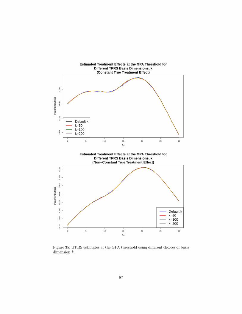
0 5 10 15 20 25 30

0.02

00.

025

0.03

00.

035

Estimated Treatment Effects at the GPA Threshold forDifferent TPRS Basis Dimensions, k

(Constant True Treatment Effect)

X2

Trea

tmen

t Effe

ct

Default kk=50k=100k=200

0 5 10 15 20 25 30

0.02

00.

025

0.03

00.

035

0.04

00.

045

0.05

00.

055

Estimated Treatment Effects at the GPA Threshold forDifferent TPRS Basis Dimensions, k

(Non−Constant True Treatment Effect)

X2

Trea

tmen

t Effe

ct


Figure 35: TPRS estimates at the GPA threshold using different choices of basisdimension k.

87

0 10 20 30 40

0.01

80.

020

0.02

20.

024

0.02

60.

028

0.03

0

Estimated Treatment Effects at the Income Threshold forDifferent TPRS Basis Dimensions, k

(Constant True Treatment Effect)

X1

Trea

tmen

t Effe

ct


0 10 20 30 40

0.02

0.03

0.04

0.05

0.06

Estimated Treatment Effects at the Income Threshold forDifferent TPRS Basis Dimensions, k

(Non−Constant True Treatment Effect)

X1

Trea

tmen

t Effe

ct


Figure 36: TPRS estimates at the income threshold using different choices ofbasis dimension k.

88

Appendix D Additional Details on TPRS

This section of the appendix provides additional details on the approximation ofthin plate splines by TPRS. Purely for simplicity of exposition, I assume for thisdiscussion that no two observations have an identical combination of covariatevalues.

Recall from section 4.3 that a thin plate spline f∗ is a solution to the followingminimization problem:

minimizef

n∑i=1

(yi − f(xi))2 + λJmd(f),

where the definition Jmd can be found in the main text. As long as the restriction2m > d is satisfied, the solution can be written as:

f∗(x) =

n∑i=1

δ∗i ηmd(||x− xi||) +

M∑j=1

α∗jφj(x),

where the orthogonality constraint T ′δ∗ = 0 is satisfied, with T defined byTij ≡ φj(xi). The functions M ≡

(m+d−1

d

)functions φj are linearly independent

polynomials that span the space of polynomials of degree less than m, and arethus not penalized at all by the penalty term Jmd. These correspond to thecomponents of “zero wiggliness” mentioned in the main text. The function ηmdis defined by:

ηmd(r) =

(−1)m+1+d/2

22m−1πd/2(m− 1)!(m− d/2)!r2m−d log(r) if d is even

Γ(d/2−m)

22mπd/2(m− 1)!r2m−d if d is odd.

Now, defining E by Eij ≡ ηmd(||xi − xj ||), the minimization problem thatdefines the thin plate spline can alternatively be written as:

(*) minimizeδ,α

||y −Eδ − Tα||2 + λδ′Eδ s.t. T ′δ = 0.

Leaving the basis for the unpenalized functions untouched, the TPRS focuseson truncating the basis for the δ parameter space in a way that perturbs theminimization problem as little as possible.

To elaborate, let k be the basis dimension for the TPRS chosen by the user.Instead of searching for the value of δ over the entire space Rn that (along withα) minimizes the objective function and satisfies the orthogonality constraint,the minimization problem that defines the TPRS only considers possible valuesof δ within a k-dimensional subspace, W of Rn.

To make precise how the subspace W is chosen for TPRS (for a given valueof k), I introduce the following notation. Given a k-dimensional subspace W of

89

Rn, let Γk be a n× k matrix of rank k with columns that form an orthonormalbasis for W . The TPRS minimization problem is thus

minimizeδk,α

||y −EΓkδk − Tα||2 + λδ′kΓ′kEΓkδk s.t. T ′Γkδk = 0,

where δ′k ∈ Rk.In order to express this in a form closer to that of the minimization problem

for the thin plate spline, I define the n × n matrices Ek ≡ EΓkΓ′k and Ek ≡

ΓkΓ′kEΓkΓ

′k. This allows me to write the TPRS minimization problem as,

(**) minimizeδ,α

||y − Ekδ − Tα||2 + λδ′Ekδ s.t. T ′δ = 0,

since δ ∈W if and only if Γkδk = δ for some δk ∈ Rk, by definition of W .Now, the goal of TPRS is to choose W , or equivalently Γk, so that replacing

the matrix E in problem (∗) by Ek and Ek in problem (∗∗) perturbs problem(∗) as little as possible. Unfortunately, there is no k-dimensional subspace thatminimizes the change in objective value for all possible values of δ. Hence,TPRS instead chooses Γk to minimize the worst possible change in objectivevalue. In other words, Γk is the orthonormal basis matrix of rank k in Rn×kthat simultaneously minimizes

εk ≡ maxδ 6=0

{||(E − Ek)δ||

||δ||

}and ek ≡ max

δ 6=0

{δ′(E − Ek)δ

||δ||2

},

where εk and ek correspond to the worst possible change in the least squaresand penalty terms respectively.

It turns out that the solution that simultaneously minimizes εk and ek is atruncated eigenbasis of E. To elaborate, write the spectral decomposition ofE as E = UDU ′ where D is the diagonal matrix containing the eigenvaluesof E, arranged in decreasing order of magnitude, i.e. |Di,i| ≥ |Di+1,i+1| fori = 1, ..., n−1.48 Then, the solution Γk is the first k columns of U , appropriatelyscaled so that the columns are orthonormal. One may also easily verify thatthis solution results in Ek = Ek.

For further details on TPRS, interested readers are encouraged to refer toWood (2003) and Wood (2006).

48This decomposition is possible because E is a real symmetric matrix by definition.

90

References

[1] Almond, Douglas, Joseph J. Doyle, Amanda E. Kowalski, and HeidiWilliams. 2010. “Estimating Marginal Returns to Medical Care: Evidence from At-risk Newborns.” The Quarterly Journal of Economics 125 (2): 591–634.

[2] Clementi, Fabio, and Mauro Gallegati. 2007. “Pareto’s Law of Income Distribu-tion: Evidence for Germany, the United Kingdom, and the United States.” In Econo-physics of Wealth Distributions, edited by Arnab Chatterjee, Sudhakar Yarlagadda,and Bikas K. Chakrabarti. Milan: Springer.

[3] Jean Duchon. 1977. “Splines minimizing rotation-invariant semi-norms in Sobolevspaces.” In Construction Theory of Functions of Several Variables, edited by WalterSchempp, and Karl Zeller. Berlin: Springer.

[4] Fan, Jianqing, and Irene Gijbels. 1992. “Variable Bandwidth and Local LinearRegression Smoothers.” The Annals of Statistics 20 (4): 2008–2036.

[5] Gelman, Andrew, and Guido W. Imbens. 2014. “Why High-order PolynomialsShould Not be Used in Regression Discontinuity Designs.” National Bureau of Eco-nomic Research Working Paper 20405.

[6] Imbens, Guido W., and Karthik Kalyanaraman. 2012. “Optimal BandwidthChoice for the Regression Discontinuity Estimator.” The Review of Economic Studies79 (3): 933–959.

[7] Imbens, Guido W., and Thomas Lemieux. 2008. “Regression discontinuity designs:A guide to practice.” Journal of Econometrics 142 (2): 615–635.

[8] Jacob, Brian A., and Lars Lefgren. 2004. “Remedial Education and StudentAchievement: A Regression-Discontinuity Analysis.” Review of Economics and Statis-tics 86 (1): 226–244.

[9] Kane, Thomas J. 2003. “A Quasi-Experimental Estimate of the Impact of FinancialAid on College-Going.” National Bureau of Economic Research Working Paper 9703.

[10] Kim, Young-Ju, and Chong Gu. 2004. “Smoothing spline Gaussian regression: morescalable computation via efficient approximation.” Journal of the Royal StatisticalSociety: Series B (Statistical Methodology) 66 (2): 337–356.

[11] Lee, David S. and David Card. 2008. “Regression discontinuity inference with spec-ification error.” Journal of Econometrics 142 (2): 655–674.

[12] Lee, David S., and Thomas Lemieux. 2010. “Regression Discontinuity Designs inEconomics.” Journal of Economic Literature 48 (2): 281–355.

[13] Ludwig, Jens, and Douglas L. Miller. 2005. “Does Head Start Improve Children’sLife Chances? Evidence from a Regression Discontinuity Design.” National Bureau ofEconomic Research Working Paper 11702.

[14] Matsudaira, Jordan D. 2008. “Mandatory summer school and student achievement.”Journal of Econometrics 142 (2): 829–850.

[15] National Center for Health Statistics. 2008. “2008 Cohort Linked Birth/InfantDeath Data Set.” United States Department of Health and Human Services.http://www.cdc.gov/nchs/data_access/vitalstatsonline.htm (accessed February21, 2016).

[16] Papay, John P., John B. Willett, and Richard J. Murnane. 2011a. “Extendingthe regression-discontinuity approach to multiple assignment variables.” Journal ofEconometrics 161 (2): 203–207.

91

[17] Papay, John P., John B. Willett, and Richard J. Murnane. 2011b. “High-SchoolExit Examinations and the Schooling Decisions of Teenagers: A Multi-DimensionalRegression-Discontinuity Analysis.” National Bureau of Economic Research WorkingPaper 17112.

[18] Patterson, Brian F., and Krista D. Mattern. 2013. “Validity of the SAT forPredicting First-Year Grades: 2010 SAT Validity Sample.” College Board StatisticalReport 2013-2. New York: The College Board.

[19] Porter, Jack. 2003. “Estimation in the Regression Discontinuity Model”. Mimeo.Department of Economics, Wisconsin. http://www.ssc.wisc.edu/~jrporter/reg_

discont_2003.pdf (accessed April 2, 2016).

[20] Rau, Tomas. 2011. “Bayesian Inference in the Regression Discontinuity Model.” Vi-gesimosextas Jornadas Anuales de Economa.

[21] Reardon, Sean F., and Joseph P. Robinson. 2012. “Regression Discontinuity De-signs With Multiple Rating-Score Variables.” Journal of Research on EducationalEffectiveness 5 (1): 83–104.

[22] Snider, Connan, and Jonathan W. Williams “Barriers to Entry in the AirlineIndustry: A multidimensional Regression-Discontinuity Analysis of AIR-21.” Reviewof Economics and Statistics 97 (5): 1002–1022.

[23] Thistlethwaite, Donald L., and Donald T. Campbell. 1960. “Regression-discontinuity analysis: An alternative to the ex post facto experiment.” Journal ofEducational Psychology 51 (6): 309–317.

[24] Wong, Vivian C., Peter M. Steiner, and Thomas D. Cook. 2013. “AnalyzingRegression-Discontinuity Designs With Multiple Assignment Variables: A Compar-ative Study of Four Estimation Methods.” Journal of Educational and BehavioralStatistics 38 (2): 107–141.

[25] Wood, Simon N. 2006. Generalized Additive Models: An Introduction with R. BocaRaton: CRC Press.

[26] Wood, Simon N. 2003. “Thin plate regression splines.” Journal of the Royal StatisticalSociety: Series B (Statistical Methodology) 65 (1): 95–114.

92

regression discontinuity designs with multiple assignment ... · pdf fileregression...

Documents