regular expressions and languages - …whtsai/course teaching affairs... · 2 outline 3.1 regular...

Chapter 3

Regular Expressions and Languages (2015/10/8)

Giza Pyramids, Egypt

2

Outline

3.1 Regular Expressions

3.2 Finite Automata & Regular Expressions

3.3 Applications of RE’s

3.4 Algebraic Laws for RE’s

3

3.1 Regular Expressions

Use of Regular expressions ---

The regular expression is a kind of generator for languages.

It offers a “declarative” way of expressing strings of symbols.

It defines all and only regular languages.

Applications of Regular expressions ---

Used as commands for finding strings in Web browsers or text-formatting systems

(such as UNIX grep commands)

Used as lexical analyzer generator (such Lex or Flex)

A lexical analyzer breaks source programs into “tokens” (keywords, identifiers,

signs, …)

3.1.1 Operators of Regular Expressions

Review of three operations on two languages L and M:

Union --- L∪M = {x | xL or xM}

Concatenation --- LM = {xy | xL, yM}

Example --- L0 = {}, L1 = L, L2 = LL, …

Closure (or star, or Kleene closure) ---

L* = L0∪L1∪L2∪...

Example 3.1 ---

* = {} because 0 = {}.

If L = {0, 1}, then L0 = {}, L1 = L, L2 = {00. 01, 10, 11}, …

If L is the set of all strings of 0’s, then it can be proved that L* is L itself (see the

textbook for the proof).

3.1.2 Building Regular Expressions

Definition ---

A regular expression (RE) E and its corresponding language L(E) are defined

recursively in the following way ---

Basis:

Constants and are RE’s defining languages {} and , respectively, which are

expressed as L() = {}, L() = .

If a is a symbol, then a is an RE defining the language {a} which may be expressed

as L(a) = {a} (note: a is of bold face).

A variable like L (capitalized and italic) represents any language.

Induction:

Given two RE’s E and F, then we have the following more complicated RE’s.

Union

E + F is an RE such that L(E + F) = L(E)∪L(F).

Concatenation

EF is an RE such that L(EF) = L(E)L(F).

Closure

E* is an RE such that L(E*) = (L(E))*.

Parenthesization

(E) is an RE such that L((E)) = L(E).

4

Example 3.2 ---

An RE defining a language of strings of alternating 0’s and 1’s is one of the two

below:

(01)* + (10)* + 0(10)

* + 1(01)

*

( + 1)(01)*( + 0)

(Why? See the textbook.)

3.1.3 Precedence of RE operators

Precedence of RE operators ---

Highest “*” (closure)

Next “.” (concatenation) (left to right)

Last “+” (union) (left to right)

Use parentheses anywhere to resolve ambiguity

Example 3.3 ---

The following are three ways to interpret the RE 01* + 1 if parentheses are not used:

(0(1*)) + 1 by precedence above;

(01)* + 1 (another meaning);

0(1* + 1) (a third meaning).

3.2 FA’s & RE’s

Theorems to be proved ---

Every language defined by a DFA is also defined by an RE.

Every language defined by an RE is also defined by an -NFA.

Relations of theorems ---

(thicker yellow arrows indicate equivalence relations to be proved in this chapter)

Fig. 3.1 Equivalence Relations among DFA’s, NFA’s, -NFA’s, and RE’s.

3.2.1 From DFA’s to RE’s

Theorem 3.4 ---

If L = L(A) for some DFA A, then there is an RE R such that L = L(R).

Proof.

Idea: the proof is conducted by constructing progressively string sets defined by a

--NNFFAA

RREE

NNFFAA

DDFFAA

5

certain RE form, Rij(k), until the entire set of acceptable strings (i.e., the language L(A))

is obtained.

Steps:

Assume that the set of states are numbered as {1, 2, ..., n} (1 is the start state).

Use the technique of induction to construct Rij(k), starting at k = 0 and stop at k = n

(the largest state number), for all i, j = 1, 2, …, n.

Meaning of RE Rij(k) ---

Rij(k) is used to denote the set of strings w such that

(1) each w is the label of a path from state i to state j in DFA A; and

(2) the path has no intermediate node whose number is larger than k.

Then, if k = n, i = 1, and j specifies an accepting state, then Rij(k) = R1j

(n) defines a

set of strings accepted by DFA A, with each string forming a path starting from the

start state (specified by i = 1) to the accepting state (specified by j).

If there are more than one accepting state, i.e., if F = {j1, j2, ..., jm} is the set of

accepting states, then all the R1j(n) so obtained for all the accepting states j = j1, j2,

…, jm are collected by union as the final result:

R1j1

(n) + R1j2

(n) + ... + R1jm

(n)

(end of the proof of theorem).

Construction of Rij(k)

by induction ---

Basis (for k = 0):

(A) When k = 0, all state numbers 1, and so there is no intermediate state in path i to j,

leading to 2 cases:

(1) an arc (a transition) from i to j;

(2) a path from i to i itself.

(B) If i j, only Case (1) is possible, leading to 3 cases:

(B1) no symbol for such a transition, indicating that Rij(0) =;

(B2) one symbol a for the transition, indicating that Rij(0) = a;

(B3) multiple symbls a1, a2, ..., am for the transition, indicating that

Rij(0) = a1 + a2 + ... + am

(C) If i = j, only Case (2) is possible, which means that there exists at least a path from i

to i itself, plus one the following 3 cases:

(C1) no symbol for such a transition, indicating that the path may be described by

Rij(0) = ;

(C2) one symbol a for the transition, indicating that the path may be described by

Rij(0) = + a;

(C3) multiple symbls a1, a2, ..., am for the transition, indicating that the path may

be described by Rij(0) = + a1 + a2 + ... + am.

Induction (for k 0):

(A) Suppose that there is a path from i to j that goes through no state numbered higher

than k. Then, two cases should be considered:

6

(1) the path does not go through k, indicating that the path is just Rij(k-1);

(2) the path goes through k at least once, meaning that the path may be broken

into 3 pieces:

(a) through i to k without passing k, meaning that this part of the path is

just Rik(k-1);

(b) from k to k itself, meaning that this part of the path may be described

by (Rkk(k-1))* (in a recursive way);

(c) from k to j without passing k, meaning that this part of the path is

Rkj(k-1),

so that the three pieces may be concatenated to be

Rik(k-1)(Rkk

(k-1))*Rkj(k-1).

(The above process may be described by the diagram shown in Fig. 3.)

(B) Combining (1) and (2) above, we get the RE defining “all the paths from i to j that

go through no state higher than k” as

Rij(k) = Rij

(k-1) + Rik(k-1)(Rkk

(k-1))*Rkj(k-1).

Fig. 3.2 Illustration of paths represented by Rij(k).

Example 3.5 ---

Convert the DFA shown in Fig. 3.3 into an RE.

Fig. 3.3 The DFA of Example 3.5.

Rij(0) may be constructed to have the results shown in Table 3.1; the details are derived

in the following.

R11(0) = + 1 because (1, 1) = 1 (going back to state 1);

R12(0) = 0 because (1, 0) = 2 (getting out to state 2);

R21(0)

= because there is no path from state 2 to 1;

k i j … …

((RRkkkk((kk--11))

))**

circulating zero or more times

RRkkjj((kk--11))

RRiikk((kk--11))

…

0, 1

1 ssttaarrtt 2

0

1

7

R22(0) = ( + 0 + 1) because (2, 0) = 2 and (2, 1) = 2 (going back to state 2).

Table 3.1 The constructed values of Rij(0) of Example 3.5.

R11

(0) + 1

R12

(0) 0

R21

(0)

R22

(0) (+ 0 + 1)

We can then compute all Rij(k) for k = 1 and k = 2.

However, we may alternatively compute only necessary terms of Rij(k) backward from

the final states, to save time.

There is only one final state, namely, 2, so we only have to compute

R12(2) = R12

(1) + R12(1)(R22

(1))*R22(1).

That is, we only have to compute R12(1) and R22

(1), without computing R21(1) and

R11(1).

To compute each of these terms, we need some RE equalities to simplify intermediate

results which we described next.

(Example 3.5 will be continued.)

Some equalities (R is an RE) ---

1. R = R = (so = annihilator for concatenation);

2. + R = R + = R (so = identity for union);

3. R = R = R (so = identity for concatenation);

4. ( + a)* = a* = (a + )*;

5. ( + a)a* = (a* + aa*) = a* + aa

* = a*;

6. a*( + a) = (a* + a*

a) = a* + a*a = a*.

(All the above equalities are theorems provable by easy deductions, which are omitted.

For details, see the textbook.)

Example 3.5 (continued) ---

To compute R12(2) = R12

(1) + R12(1)(R22

(1))*R22(1), we have the following derivations.

R12(1) = R12

(0) + R11(0)(R11

(0))*R12(0)

= 0 + ( + 1)( + 1)*0 (by substitutions)

= 0 + ( + 1)1*0 (by Equality 4 above)

= 0 + 1* 0 (by Equality 5 above)

= ( + 1*)0 (by the distributive law)

= 1*0 (by Equality 4 above)

R22(1) = R22

(0) + R21(0)(R11

(0))*R12(0)

= ( + 0 + 1) + ( + 1)*0 (by substitutions)

= ( + 0 + 1) + (by Equality 1 above)

= + 0 + 1 (by Equality 2 above)

8

Finally, R12(2) may be computed as follows.

R12(2) = 1

*0 +1

*0( + 0 + 1)

*( + 0 + 1) (by subst.)

= 1*0 +1

*0(0 + 1)

*( + 0 + 1) (by Equality 4 above)

= 1*0 +1

*0(0 + 1)

* (by Equality 6 above)

= 1*0( + (0 + 1)*) (by the distributive law)

= 1*0(0 + 1)

* (by Equality 4 above)

The correctness of the final result R12(2) = 1*

0(0 + 1)* may checked by inspecting the

transition diagram shown in Fig. 3.3.

The above method also works for the NFA and the -NFA.

3.2.2 Converting DFA’s to RE’s by State Elimination

Idea ---

Step 1 – regard symbols on arcs as RE’s;

Step 2 – conduct each of the type of conversion as illustrated by Fig. 3.4;

Step 3 – collect RE’s for all the final states.

Fig. 3.4 Illustration of converting DFA’s to RE’s by eliminating states (for a complete diagram, see the textbook).

Details of Step 3 ---

For each final state q, eliminate all the states as illustrated in Fig. 3.4 except the start

state q0.

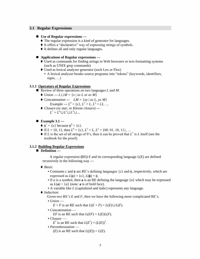
If q q0, then a 2-state automaton is left as shown in Fig. 3.5 (Fig. 3.9 in the textbook),

whose corresponding RE may be shown to be (R+SU*T)*SU* (provable by the type of

conversion described in Fig. 3.4).

S q1 q2

s

R11

Q1 P1

. . .

. . .

q1 q2

R11+ Q1S*P1

. . .

. . .

Fig. 3.7 in textbook (partial) Fig. 3.8 in textbook (partial)

9

Fig. 3.5 The first type of partial result of Step 2 a 2-state automaton.

If q = q0, then perform one more state elimination to eliminate q, leaving only the start

state q0 as shown in Fig. 3.6 (also, see an example later). The corresponding RE is R*.

Collect the result for each final state derived as above to get the final result.

Fig. 3.6 The first type of partial result of Step 2.

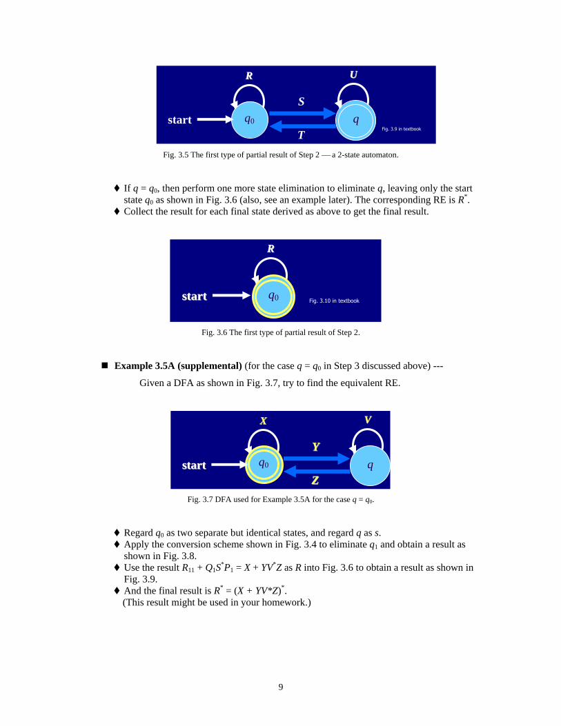
Example 3.5A (supplemental) (for the case q = q0 in Step 3 discussed above) ---

Given a DFA as shown in Fig. 3.7, try to find the equivalent RE.

Fig. 3.7 DFA used for Example 3.5A for the case q = q0.

Regard q0 as two separate but identical states, and regard q as s.

Apply the conversion scheme shown in Fig. 3.4 to eliminate q1 and obtain a result as

shown in Fig. 3.8.

Use the result R11 + Q1S*P1 = X + YV*Z as R into Fig. 3.6 to obtain a result as shown in

Fig. 3.9.

And the final result is R* = (X + YV*Z)*.

(This result might be used in your homework.)

UU RR

qq00 qq

S

T

start Fig. 3.9 in textbook

RR

qq00 ssttaarrtt Fig. 3.10 in textbook

VV XX

qq00 qq

YY

ZZ

ssttaarrtt

10

Fig. 3.8 Process for obtaining the RE for the DFA of Example 3.5A shown in Fig 3.7.

Fig. 3.9 The final result for obtaining the RE for the DFA of Example 3.5A shown in Fig 3.7.

Example 3.5 revisited (solved by state elimination) ---

Use the state elimination scheme to obtain the RE for the DFA of Example 3.5 (not

Example 3.5A) shown in Fig. 3.3 (which is repeated below).

Fig. 3.3 The DFA of Example 3.5 (repeated here for viewing convenience).

Use the derivation for 2-state automaton described previously (shown in Fig. 3.5 and

repeated below) directly to get R = 1, S = 0, T = , U = 0 + 1.

Fig. 3.5 The first type of partial result of Step 2 a 2-state automaton (repeated here for viewing convenience).

UU RR

qq00 qq

S

T


0, 1

1 ssttaarrtt 2

0

1

S= V q0 q0

s

R11=X

Q1=Y P1=Z

. . .

. . .

q0 q0

R11+ Q1S*P1

=X+YV*Z

. . .

. . . RR==XX ++ YYVV**ZZ

qq00 ssttaarrtt

Fig. 3.7 in textbook (partial) Fig. 3.8 in textbook (partial)

11

The desired result is:

(R+SU*T)*SU* = (1 + 0(0 + 1)*)*0(0 + 1)*

= 1* 0(0 + 1)*.

The same as derived before. Correct!

Example 3.6 ---

Use the state elimination scheme to obtain the RE for the NFA shown in Fig. 3.9.

Fig. 3.9 NFA of Example 3.6.

Step 1: regard all symbols on the arcs as RE’s, we get a result as shown in Fig. 3.10.

Fig. 3.10 Result of Step 1 of Example 3.6.

Step 2: to remove B, applying the state-elimination conversion shown in Fig. 3.11 (a

repetition of Fig. 3.4), we get s = B, q1 = A, q2 = C, S = , Q1 = 1, P1 = 0 + 1, R11 = so

that

R11 + Q1S*P1 = + 1*(0 + 1) = 1(0 + 1) = 1(0 + 1).

And the resulting intermediate NFA is as shown in Fig. 3.12.

Fig. 3.11 A repetition of Fig. 3.4.

A ssttaarrtt B

1

0, 1

C

0, 1 D

0, 1

C A ssttaarrtt B

1

0 + 1

0 + 1 D

0 + 1

S q1 q2

s

R11

Q1 P1

. . .

. . .

q1 q2

R11+ Q1S *P1

. . .

. . .

12


Step 3: for the final state D, we have to remove C further using the conversion shown

in Fig. 3.11 again, resulting in s = C, q1 = A, q2 = D, S = Q1 =1(0 + 1), P1 =0 + 1, R11=

, so that

R11 + Q1S*P1 = + 1(0 + 1)*(0 + 1) = 1(0 + 1)(0 + 1).



Step 4: by the conversion using the 2-state automaton shown in Fig. 3.13 (a repetition

of Fig. 3.5), we get R = (0 + 1), q1 = A, q2 = D, S = 1(0 + 1)(0 + 1), T = , U = so that

(R+SU*T)*SU* = (0 + 1 + 1(0 + 1)*)*(1(0 + 1)(0 + 1)) *

= (0 + 1)*1(0 + 1)(0 + 1).


Fig. 3.13 A repetition of Fig. 3.5 a 2-state automaton (repeated here for viewing convenience).


UU RR

qq00 qq

S

T


A ssttaarrtt

0 + 1

C

1(0 + 1) D

0 + 1

A ssttaarrtt

0 + 1

11((00 ++ 11))((00 ++ 11))

D

A ssttaarrtt

0 + 1

11((00 ++ 11))((00 ++ 11))

D

13

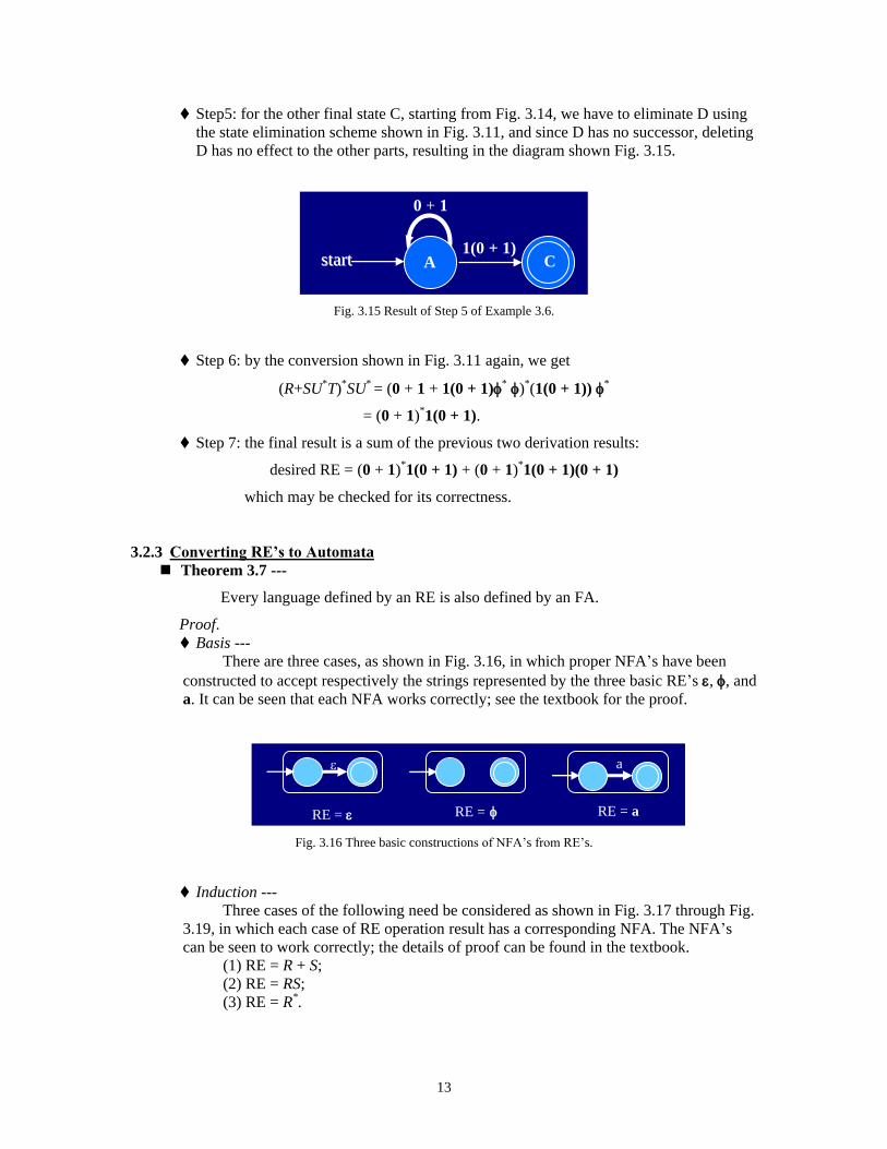
Step5: for the other final state C, starting from Fig. 3.14, we have to eliminate D using

the state elimination scheme shown in Fig. 3.11, and since D has no successor, deleting

D has no effect to the other parts, resulting in the diagram shown Fig. 3.15.


Step 6: by the conversion shown in Fig. 3.11 again, we get

(R+SU*T)*SU* = (0 + 1 + 1(0 + 1)*)*(1(0 + 1))*

= (0 + 1)*1(0 + 1).

Step 7: the final result is a sum of the previous two derivation results:

desired RE = (0 + 1)*1(0 + 1) + (0 + 1)*

1(0 + 1)(0 + 1)

which may be checked for its correctness.

3.2.3 Converting RE’s to Automata

Theorem 3.7 ---

Every language defined by an RE is also defined by an FA.

Proof.

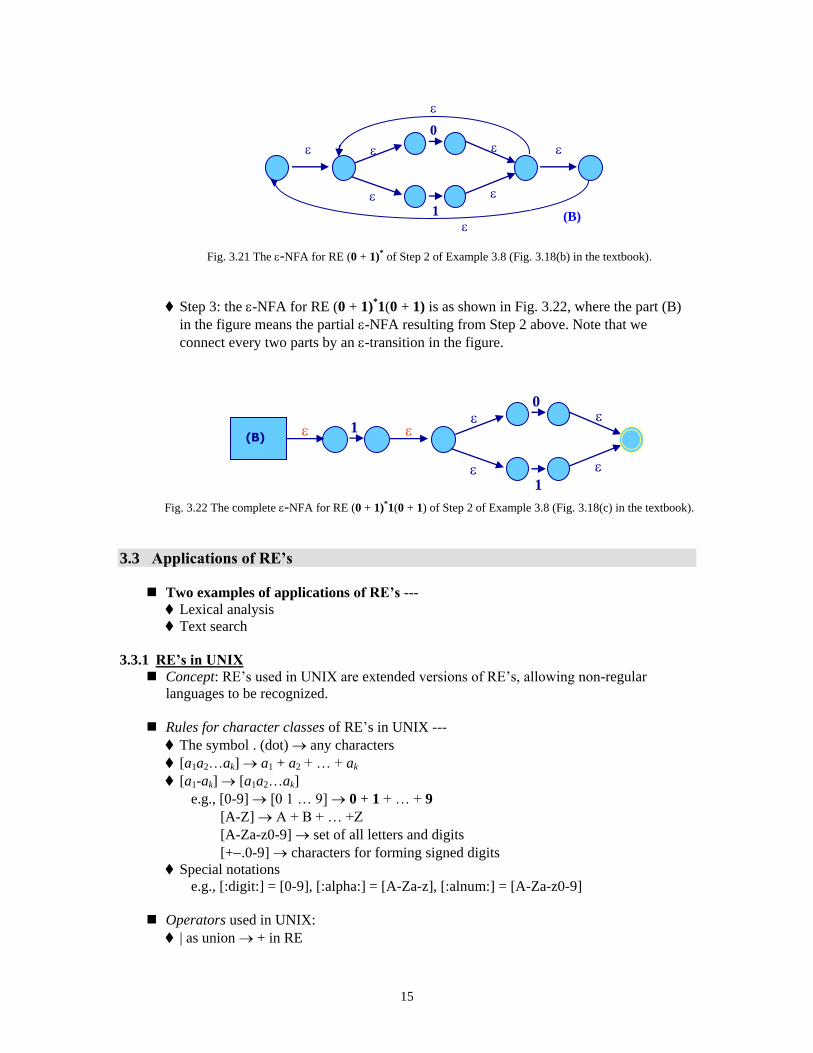
Basis ---

There are three cases, as shown in Fig. 3.16, in which proper NFA’s have been

constructed to accept respectively the strings represented by the three basic RE’s , , and

a. It can be seen that each NFA works correctly; see the textbook for the proof.

Fig. 3.16 Three basic constructions of NFA’s from RE’s.

Induction ---

Three cases of the following need be considered as shown in Fig. 3.17 through Fig.

3.19, in which each case of RE operation result has a corresponding NFA. The NFA’s

can be seen to work correctly; the details of proof can be found in the textbook.

(1) RE = R + S;

(2) RE = RS;

(3) RE = R*.

A ssttaarrtt

0 + 1

C

1(0 + 1)

RE = RE =

a

RE = a

14

Fig. 3.17 NFA for RE operation R + S.

Fig. 3.18 NFA for RE operation RS.

Fig. 3.19 NFA for RE operation R*.

Example 3.8 ---

Convert RE (0 + 1)*1(0 + 1) into an -NFA.

Step 1: the -NFA for RE 0 + 1 is as shown in Fig. 3.20.

Fig. 3.20 The -NFA for RE 0 + 1 of Step 1 of Example 3.8 (Fig. 3.18(a) in the textbook).

Step 2: the -NFA for RE (0 + 1)* is as shown in Fig. 3.21.

RE = R + S

R

S

RE = RS

R

S

RE = R*

R

R0

0

1

15

Fig. 3.21 The -NFA for RE (0 + 1)

* of Step 2 of Example 3.8 (Fig. 3.18(b) in the textbook).

Step 3: the -NFA for RE (0 + 1)*1(0 + 1) is as shown in Fig. 3.22, where the part (B)

in the figure means the partial -NFA resulting from Step 2 above. Note that we

connect every two parts by an -transition in the figure.

Fig. 3.22 The complete -NFA for RE (0 + 1)

*1(0 + 1) of Step 2 of Example 3.8 (Fig. 3.18(c) in the textbook).

3.3 Applications of RE’s

Two examples of applications of RE’s ---

Lexical analysis

Text search

3.3.1 RE’s in UNIX

Concept: RE’s used in UNIX are extended versions of RE’s, allowing non-regular

languages to be recognized.

Rules for character classes of RE’s in UNIX ---

The symbol . (dot) any characters

[a1a2…ak] a1 + a2 + … + ak

[a1-ak] [a1a2…ak]

e.g., [0-9] [0 1 … 9] 0 + 1 + … + 9

[A-Z] A + B + … +Z

[A-Za-z0-9] set of all letters and digits

[+.0-9] characters for forming signed digits

Special notations

e.g., [:digit:] = [0-9], [:alpha:] = [A-Za-z], [:alnum:] = [A-Za-z0-9]

Operators used in UNIX:

| as union + in RE

0

1

(B)

0

1

1 (B)

16

? as “zero or one of”

e.g., R? + R

+ as “one or more of”

e.g., R+ RR* (= R+)

{n} as “n copies of”

e.g., R{5} RRRRR (= R5)

* still used in UNIX with the same meaning

3.3.2 Lexical analysis

An example recalled (in Chapter 1) ---

’[A-Z][a-z]*[ ][A-Z][A-Z]’ means the following RE:

(A+B+…+Z)(a+b+…+z)*_(A+B+…Z)(A+B+…+Z)

where _ means a blank.

The above can be used to represent addresses like Ithaca NY, Buffalo NY, …

UNIX commands ---

Each UNIX command lex or flex for lexical analysis has the following form:

UNIX-style RE {code for lexical analyzer generation;}

Examples --- else {return(ELSE);}

[A-Za-z][A-Za-z0-9]* {code to enter the found identifier in the

symbol table; return(ID);}

>= {return(GE);}

…

3.3.3 Finding Patterns in Text

Concept: we can use RE’s in UNIX for pattern search in Web pages.

An example:

UNIX RE’s for addresses (incomplete) are of the following form:

’[0-9]+[A-Z]?[ ][A-Z][a-z]*([ ][A-Z][a-z]*)*[ ] (Street|St\.|Avenue|Ave\.|Road |Rd\.)’

e.g., 123A Main Street, 20 Ta Hsueh Rd., …

Notes:

There is inconsistency in textbook; blanks should be replaced by [ ] (see p. 4 & p. 113

in the textbook)

The backslash is used to differentiate a real dot from the dot used for ‘any character’)

3.4 Algebraic Laws for RE’s

Purpose of this section: to derive “high-level” algebraic laws for equivalent RE’s

Definition: two RE’s are said to be equivalent if the languages they define are identical.

17

A note: the RE’s to be discussed include variables, instead of just constants like , 0, 1, a,

01, …

3.4.1 Associativity and Commutativity

Assume that L, M, and N are RE’s (variables). Some equalities involving associativity

and commutativity are as follows.

Commutative law for union ---

L + M = M + L

Associative law for union ---

(L + M) + N = L + (M + N)

Associative law for concatenation ---

(LM)N = L(MN)

(Note: the commutative law for concatenation is false.)

3.4.2 Identities and Annihilators

There are some equalities involving the concepts of identity and annihilator as follows.

(Note: identity --- a component absorbed by another after some operation is conducted;

annihilator --- a component causing another to cease to exist after some operation is

conducted.)

identity for union ( + L = L + = L)

U annihilator for union ( U + L = L + U = U)

identity for concatenation ( L = L = L)

annihilator for concatenation ( L = L = )

(Note: means “because.”)

3.4.3 Distributive Laws

There are two equalities involving distributiveness, which are as follows.

Left distributive law of concatenation over union ---

L(M + N) = LM + LN

Right distributive law of concatenation over union ---

(M + N)L = ML + NL

(Note: U denotes the universal language.)

3.4.4 The Idempotent Law

The idempotent law for union ---

L + L = L

(Note: “idempotent” means “relating to or being a mathematical quantity which when

applied to itself under a given binary operation (as multiplication) equals itself”;【數】冪

等(的); 等冪(的).)

18

3.4.5 Laws Involving Closures

There are a few equalities involving the operation of closure as follows.

(L*)* = L*

* =

* =

L+ = L*L = LL*

(L + M)* = (L*M*)*

L* = L+ + (easy)

L? = + L (the definition of ? were given before)

(For the proofs, see the textbook.)

(Read Sections 3.4.6 & 3.4.7 by yourself.)

3.4.7a Some RE Equalities (supplemental)

There are more RE equalities which are useful for RE simplification as follows, where p,

q, and r are RE’s.

* = * =

rr* = r*r

r* = r*r* = (r*)* = r* + r*

r* = + rr* = + r*r = + r* = ( + r)* = ( + r)r*

r* = (r + r2 + … +rk)* (k 1)

r* = + r + r2 + … + rk - 1 + rkr* (k 1)

(p + q)* = (p* + q*)* = (p*q*)* = p*(qp*)* = (p*q)*p*

(pq)*p = p(qp)*

(p*q)* = + (p + q)*q (pq*)* = + p(p + q)*

(For proofs, see the text and exercises of Chapter 6 in my Chinese textbook)

.

.. .

regular expressions and languages - …whtsai/course teaching affairs... · 2 outline 3.1 regular...

Documents