Lehmann `04 1

RegularRegular Variation and Financial Time Series ModelsVariation and Financial Time Series Models

Richard A. DavisColorado State University

www.stat.colostate.edu/~rdavis

Thomas MikoschUniversity of Copenhagen

Bojan BasrakEurandom

Lehmann `04 2

Outline

Characteristics of some financial time seriesIBM returnsMultiplicative models for log-returns (GARCH, SV)

Regular variationunivariate casemultivariate casenew characterization: X is RV ⇔ c´X is RV ?

Applications of regular variationStochastic recurrence equations (GARCH)Point process convergenceExtremes and extremal indexLimit behavior of sample correlations

Wrap-up

Lehmann `04 3

Characteristics of some financial time series

Define Xt = ln (Pt) - ln (Pt-1) (log returns)

• heavy tailed

P(|X1| > x) ~ C x−α, 0 < α < 4.

• uncorrelated

near 0 for all lags h > 0 (MGD sequence)

• |Xt| and Xt2 have slowly decaying autocorrelations

converge to 0 slowly as h increases.

• process exhibits ‘volatility clustering’.

)(ˆ hXρ

)(ˆ and )(ˆ 2|| hhXX ρρ

Lehmann `04 4

Log returns for IBM 1/3/62-11/3/00 (blue=1961-1981)

1962 1967 1972 1977 1982 1987 1992 1997

time

-20

-10

010

100*

log(

retu

rns)

Lehmann `04 5

Sample ACF IBM (a) 1962-1981, (b) 1982-2000

0 10 20 30 40

Lag

0.0

0.2

0.4

0.6

0.8

1.0

AC

F

(a) ACF of IBM (1st half)

0 10 20 30 40

Lag

0.0

0.2

0.4

0.6

0.8

1.0

AC

F

(b) ACF of IBM (2nd half)

Lehmann `04 7

Sample ACF of squares for IBM (a) 1961-1981, (b) 1982-2000

0 10 20 30 40

Lag

0.0

0.2

0.4

0.6

0.8

1.0

AC

F

(a) ACF, Squares of IBM (1st half)

0 10 20 30 40

Lag

0.0

0.2

0.4

0.6

0.8

1.0

AC

F

(b) ACF, Squares of IBM (2nd half)

Lehmann `04 8

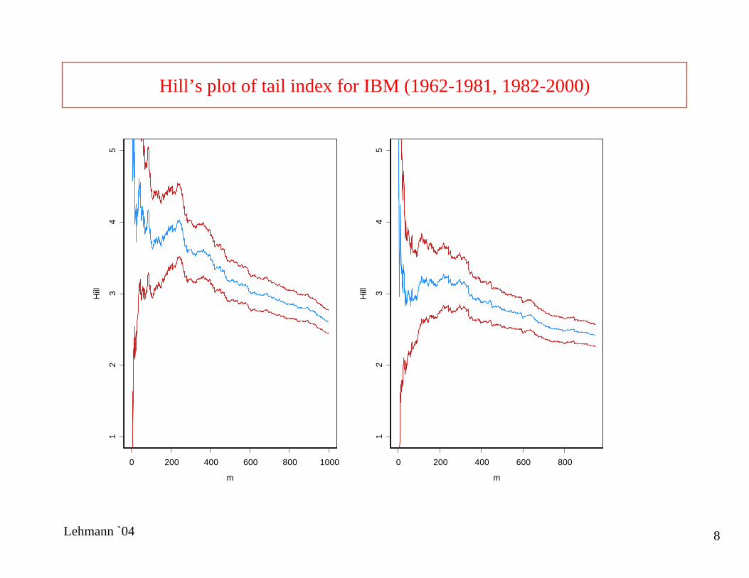
Hill’s plot of tail index for IBM (1962-1981, 1982-2000)

0 200 400 600 800 1000

m

12

34

5

Hill

0 200 400 600 800

m

12

34

5

Hill

Lehmann `04 9

Multiplicative models for log(returns)

Basic model

Xt = ln (Pt) − ln (Pt-1) (log returns)= σt Zt ,

where• {Zt} is IID with mean 0, variance 1 (if exists). (e.g. N(0,1) ora t-distribution with ν df.)

• {σt}is the volatility process

• σt and Zt are independent.

Properties:

• EXt = 0, Cov(Xt, Xt+h) = 0, h>0 (uncorrelated if Var(Xt) < ∞)

• conditional heteroscedastic (condition on σt).

Lehmann `04 10

Multiplicative models for log(returns)-cont

Xt = σt Zt (observation eqn in state-space formulation)

Two classes of models for volatility:

(i) GARCH(p,q) process (General AutoRegressive ConditionalHeteroscedastic-observation-driven specification)

Special case: ARCH(1):

(stochastic recursion eqn)

. XX 2q-t

21-t1

2p-t

21-t10

2t σβ++σβ+α++α+α=σ qp LL

t2

1-tt

2t0

21-t

2t1

2t

21-t10

2t

BXA

ZXZ

Z)X(X

+=

α+α=

α+α=

.3/1 if , )( 21

h12 <= ααρ hX

Lehmann `04 12

Multiplicative models for log(returns)-cont

Xt = σt Zt (observation eqn in state-space formulation)

(ii) stochastic volatility process (parameter-driven specification)

)N(0, IID~}{ , ,log 222 σεψεψσ tj

jjtj

jt ∞<= ∑∑∞

−∞=−

∞

−∞=

41

22 /),( )( 2 EZCorh httX +σσ=ρ

Question:

• Joint distributions of process regularly varying if distr of Z1 is regularly varying?

Lehmann `04 13

Regular variation — univariate case

Definition: The random variable X is regularly varying with index α if

P(|X|> t x)/P(|X|>t) → x−α and P(X> t)/P(|X|>t) →p,

or, equivalently, if

P(X> t x)/P(|X|>t) → px−α and P(X< −t x)/P(|X|>t) → qx−α ,

where 0 ≤ p ≤ 1 and p+q=1.

Equivalence:X is RV(α) if and only if P(X ∈ t • ) /P(|X|>t)→v µ(• )

(→v vague convergence of measures on RR\{0}). In this case,

µ(dx) = (pα x−α−1 I(x>0) + qα (-x)-α−1 I(x<0)) dx

Note: µ(tA) = t-α µ(A) for every t and A bounded away from 0.

Lehmann `04 14

Regular variation — univariate case

Another formulation (polar coordinates):

Define the ± 1 valued rv θ, P(θ = 1) = p, P(θ = −1) = 1− p = q.Then

X is RV(α) if and only if

or

(→v vague convergence of measures on SS0= {-1,1}).

)(x)t |X(|

)|X|X/ t x, |X(| SPP

SP∈→

>∈> α− θ

)(x)t |X(|

)|X|X/ t x, |X(|•∈→

>•∈> α− θP

PP

v

Lehmann `04 15

Equivalence:

µ is a measure on RRm which satisfies for x > 0 and A bounded away from 0,

µ(xB) = x−α µ(xA).

Regular variation—multivariate case

Multivariate regular variation of X=(X1, . . . , Xm): There exists a random vector θ ∈ Sm-1 such that

P(|X|> t x, X/|X| ∈ • )/P(|X|>t) →v x−α P( θ ∈ • )

(→v vague convergence on SSm-1, unit sphere in Rm) .

• P( θ ∈•) is called the spectral measure

• α is the index of X.

)()t |(|)t (

•µ→>

•∈vP

PXX )(

)t |(|)t (

•µ→>

•∈vP

PXX

Lehmann `04 16

1. If X1> 0 and X2 > 0 are iid RV(α), then X= (X1, X2 ) is multivariate regularly varying with index α and spectral distribution

P( θ =(0,1) ) = P( θ =(1,0) ) =.5 (mass on axes).

Interpretation: Unlikely that X1 and X2 are very large at the same time.

0 5 10 15 20

x_1

010

2030

40

x_2

Examples

Figure: plot of (Xt1,Xt2) for realization of 10,000.

Lehmann `04 17

2. If X1 = X2 > 0, then X= (X1, X2 ) is multivariate regularly varying with index α and spectral distribution

P( θ = (1/√2, 1/√2) ) = 1.

3. AR(1): Xt= .9 Xt-1 + Zt , {Zt}~IID symmetric stable (1.8)

±(1,.9)/sqrt(1.81), W.P. .9898

±(0,1), W.P. .0102{

-10 0 10 20 30x_t

-10

010

2030

x_{t+

1}

Figure: plot of (Xt, Xt+1) for realization of 10,000.

Distr of θ:

Lehmann `04 18

Applications of multivariate regular variation

• Domain of attraction for sums of iid random vectors (Rvaceva, 1962). That is, when does the partial sum

converge for some constants an?

• Spectral measure of multivariate stable vectors.

• Domain of attraction for componentwise maxima of iidrandom vectors (Resnick, 1987). Limit behavior of

• Weak convergence of point processes with iid points.

• Solution to stochastic recurrence equations, Y t= At Yt-1 + Bt

• Weak convergence of sample autocovariance.

∑=

−n

tna

1t

1 X

t1

1 Xn

tna=

− ∨

Lehmann `04 20

Use vague convergence with Ac={y: cTy > 1}, i.e.,

where t-αL(t) = P(|X| > t).

RV Equivalence — linear combinations

Linear combinations:

X ~RV(α) ⇒ all linear combinations of X are regularly varying

),(w:)A()t |(|)t (

)()tA ( T

cX

XcXc

c =µ→>>

=∈

α− PP

tLtP

i.e., there exist α and slowly varying fcn L(.), s.t.

P(cTX> t)/(t-αL(t)) →w(c), exists for all real-valued c,

where

w(tc) = t−αw(c).

Ac),(w:)A(

)t |(|)t (

)()tA ( T

cX

XcXc

c =µ→>>

=∈

α− PP

tLtP

Lehmann `04 21

RV Equivalence — linear combinations (cont)

Converse?

X ~RV(α) ⇐ all linear combinations of X are regularly varying?

There exist α and slowly varying fcn L(.), s.t.

(LC) P(cTX> t)/(t-αL(t)) →w(c), exists for all real-valued c.

Theorem. Let X be a random vector.

1. If X satisfies (LC) with α non-integer, then X is RV(α).

2. If X > 0 satisfies (LC) for non-negative c and α is non-integer, then X is

RV(α).

3. If X > 0 satisfies (LC) with α an odd integer, then X is RV(α).

Lehmann `04 23

Applications of theorem

1. Kesten (1973). Under general conditions, (LC) holds with L(t)=1 for

stochastic recurrence equations of the form

Yt= At Yt-1+ Bt, (At , Bt) ~ IID,

At d×d random matrices, Bt random d-vectors.

It follows that the distributions of Yt, and in fact all of the finite dim’l distrs of Yt

are regularly varying (if α is non-even).

2. GARCH processes. Since squares of a GARCH process can be embedded in a

SRE, the finite dimensional distributions of a GARCH are regularly varying.

Lehmann `04 25

Example: ARCH(1) model Xt=(α0+α1 X2t-1)1/2Zt

Figures: plots of (Xt, Xt+1) and estimated distribution of θ for realization of 10,000.

Example of ARCH(1): α0=1, α1=1, α=2

-20 -10 0 10 20

x_t

-20

-10

010

20

x_{t+

1}

-3 -2 -1 0 1 2 3

theta

0.06

0.08

0.10

0.12

0.14

0.16

0.18

Lehmann `04 26

Example: SV model Xt = σt Zt

Suppose Zt ~ RV(α) and

Then Zn=(Z1,…,Zn)’ is regulary varying with index α and so is

Xn= (X1,…,Xn)’ = diag(σ1,…, σn) Zn

with spectral distribution concentrated on (±1,0), (0, ±1).

).N(0, IID~}{ , ,log 222 σε∞<ψεψ=σ ∑∑∞

−∞=−

∞

−∞=t

jjjt

jjt

-5000 0 5000 10000

x_1

-500

00

5000

1000

0

x_2

Figure: plot of (Xt,Xt+1) for realization of 10,000.

Lehmann `04 28

Point process convergence

Theorem (Davis & Hsing `95, Davis & Mikosch `97). Let {Xt} be a stationary sequence of random m-vectors. Suppose

(i) finite dimensional distributions are jointly regularly varying (let (θ−k, . . . , θk)be the vector in S(2k+1)m-1 in the definition).

(ii) mixing condition A (an) or strong mixing.

(iii)

Then

(extremal index)

exists. If γ > 0, then

.0) || ||(suplimlim 0t||=>>∨

≤≤∞→∞→yayaP nnrtknk n

XX

α+=

α

∞→θθ∨−θ=γ || /) |||(|lim )(

0)(

1

)(0

kkjj

kk

kEE

,::111

/ ijt ∑∑∑∞

=

∞

==

ε=⎯→⎯ε=j

Pi

dn

tan in

NN QX

Lehmann `04 29

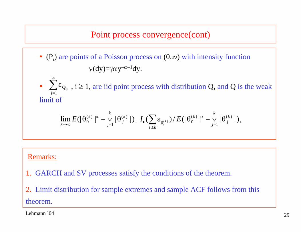
Point process convergence(cont)

• (Pi) are points of a Poisson process on (0,∞) with intensity functionν(dy)=γαy−α−1dy.

• , i ≥ 1, are iid point process with distribution Q, and Q is the weak

limit of

∑∞

=

ε1

ijj

Q

∑≤

+=

αθ•+=

α

∞→θ∨−θεθ∨−θ

kt

kjj

kkk

jj

kk

kEIE k

t||

)(

1

)(0

)(

1

)(0 ) |||(|/)( ) |||(|lim )(

Remarks:

1. GARCH and SV processes satisfy the conditions of the theorem.

2. Limit distribution for sample extremes and sample ACF follows from this theorem.

Lehmann `04 30

Extremes for GARCH & SV Processes

Setup

Xt = σt Zt , {Zt} ~ IID (0,1)

Xt is RV (α)

Choose {bn} s.t. nP(Xt > bn) →1

Then }.exp{)( 1

1 α−− −→≤ xxXbP nn

Then, with Mn= max{X1, . . . , Xn},

(i) GARCH:

γ is extremal index ( 0 < γ < 1).

(ii) SV model:

extremal index γ = 1 no clustering.

},exp{)( 1 α−− γ−→≤ xxMbP nn

},exp{)( 1 α−− −→≤ xxMbP nn

Lehmann `04 31

Extremes for GARCH & SV Processes (cont)

(i) GARCH:

(ii) SV model:

}exp{)( 1 α−− γ−→≤ xxMbP nn

}exp{)( 1 α−− −→≤ xxMbP nn

Remarks about extremal index.

(i) γ < 1 implies clustering of exceedances

(ii) Numerical example. Suppose c is a threshold such that

Then, if γ = .5,

(iii) 1/γ is the mean cluster size of exceedances.

(iv) Use γ to discriminate between GARCH and SV models.

(v) Even for the light-tailed SV model (i.e., {Zt} ~IID N(0,1), the extremalindex is 1 (see Breidt and Davis `98 )

95.~)( 11 cXbP n

n ≤−

975.)95(.~)( 5.1 =≤− cMbP nn

Lehmann `04 32

Extremes for GARCH & SV Processes (cont)

0 20 40 60

time

010

2030

0 20 40 60

time

010

2030

** * * *** ***

Lehmann `04 33

Summary for ACF of GARCH(p,q)

α∈(0,2):

α∈(2,4):

α∈(4,∞):

Remark: Similar results hold for the sample ACF based on |Xt| and Xt2.

,)/())(ˆ( ,,10,,1 mhhd

mhX VVh KK == ⎯→⎯ρ

( ) ( ) .)0()(ˆ ,,11

,,1/21

mhhXd

mhX VhnKK =

−=

α− γ⎯→⎯ρ

( ) ( ) .)0()(ˆ ,,11

,,12/1

mhhXd

mhX GhnKK =

−= γ⎯→⎯ρ

Lehmann `04 34

Summary of ACF for SV

α∈(0,2):

α∈(2, ∞):

( ) ( ) .)0()(ˆ ,,11

,,12/1

mhhXd

mhX GhnKK =

−= γ⎯→⎯ρ

( ) .)(ˆln/0

21

1h1/1

SShnn hd

X

α

α+α

σ

σσ⎯→⎯ρ

Lehmann `04 35

Sample ACF for GARCH and SV Models (1000 reps)-0

.3-0

.10.

10.

3

(a) GARCH(1,1) Model, n=10000

-0.0

6-0

.02

0.02

(b) SV Model, n=10000

Lehmann `04 36

Sample ACF for Squares of GARCH (1000 reps)

(a) GARCH(1,1) Model, n=100000.

00.

20.

40.

60.

00.

20.

40.

6

b) GARCH(1,1) Model, n=100000

Lehmann `04 37

Sample ACF for Squares of SV (1000 reps)0.

00.

010.

020.

030.

04

(d) SV Model, n=100000

0.0

0.05

0.10

0.15

(c) SV Model, n=10000

Lehmann `04 38

Wrap-up

• Regular variation is a flexible tool for modeling both dependence and tail

heaviness.

• Useful for establishing point process convergence of heavy-tailed time series.

• Extremal index γ < 1 for GARCH and γ =1 for SV.

Unresolved issues related to RV⇔ (LC)

• α = 2n?

• there is an example for which X1, X2 > 0, and (c, X1) and (c, X2) have the same limits for all c > 0.

• α = 2n−1 and X > 0 (not true in general).