regularization of wavelet approximationsorfe.princeton.edu/~jqfan/papers/01/rose.pdf ·...
TRANSCRIPT

Regularization of Wavelet ApproximationsAnestis Antoniadis and Jianqing Fan
In this paper we introduce nonlinear regularized wavelet estimators for estimating nonparametric regression functions when samplingpoints are not uniformly spaced The approach can apply readily to many other statistical contexts Various new penalty functions areproposed The hard-thresholding and soft-thresholding estimators of Donoho and Johnstone are speci c members of nonlinear regularizedwavelet estimators They correspond to the lower and upper envelopes of a class of the penalized least squares estimators Necessaryconditions for penalty functions are given for regularized estimators to possess thresholding properties Oracle inequalities and universalthresholding parameters are obtained for a large class of penalty functions The sampling properties of nonlinear regularized waveletestimators are established and are shown to be adaptively minimax To ef ciently solve penalized least squares problems nonlinearregularized Sobolev interpolators (NRSI) are proposed as initial estimators which are shown to have good sampling properties TheNRS I is further ameliorated by regularized one-step estimators which are the one-step estimators of the penalized least squares problemsusing the NRSI as initial estimators The graduated nonconvexit y algorithm is also introduced to handle penalized least squares problemsThe newly introduced approaches are illustrated by a few numerical examples
KEY WORDS Asymptotic minimax Irregular designs Nonquadrati c penality functions Oracle inequalities Penalized least-squaresROSE Wavelets
1 INTRODUCTION
Wavelets are a family of orthogonal bases that can effec-tively compress signals with possible irregularities Theyare good bases for modeling statistical functions Variousapplications of wavelets in statistics have been made in theliterature See for example Donoho and Johnstone (1994)Antoniadis Greacutegoire and McKeague (1994) Hall and Patil(1995) Neumann and Spokoiny (1995) Antoniadis (1996)and Wang (1996) Further references can be found in thesurvey papers by Donoho et al (1995) Antoniadis (1997)and Abramovich Bailey and Sapatinas (2000) and books byOgden (1997) and Vidakovic (1999) Yet wavelet applicationsto statistics are hampered by the requirements that the designsare equispaced and the sample size be a power of 2 Variousattempts have been made to relax these requirements See forexample the interpolation method of Hall and Turlach (1997)the binning method of Antoniadis Greacutegoire and Vial (1997)the transformation method of Cai and Brown (1997) the iso-metric method of Sardy et al (1999) and the interpolationmethod to a ne regular grid of Kovac and Silverman (2000)However it poses some challenges to extend these methods toother statistical contexts such as generalized additive modelsand generalized analysis of variance models
In an attempt to make genuine wavelet applications to statis-tics we approach the denoising problem from a statisticalmodeling point of view The idea can be extended to other sta-tistical contexts Suppose that we have noisy data at irregulardesign points 8t11 1 tn9
Yi D f 4ti5 C ˜i1 ˜i
iidN 401lsquo 251
Anestis Antoniadis is Professor Laboratoire de Modeacutelisation et CalculUniversiteacute Joseph Fourier 38041 Grenoble Cedex 9 France Jianqing Fan isProfessor of Statistics and Chairman Department of Statistics The ChineseUniversity of Hong Kong Shatin Hong Kong Antoniadisrsquos research wassupported by the IDOPT project INRIA-CNRS- IMAG Fanrsquos research waspartially supported by NSF grants DMS-9803200 DMS-9977096 and DMS-0196041 and RGC grant CUHK-429900P of HKSAR The major part of theresearch was conducted while Fan visited the Universiteacute Joseph Fourier Heis grateful for the generous support of the university The authors thank ArneKovac and Bernard Silverman for providing their Splus procedure makegridrequired for some of the data analyses The Splus procedure is availableat httpwwwstatmathematikuni-essende Qkovacmakegridtar The authorsthank the editor the associate editor and the referees for their commentswhich substantially improved this article
where f is an unknown regression to be estimated from thenoisy sample Without loss of generality assume that thefunction f is de ned on 601 17 Assume further that ti D ni=2J
for some ni and some ne resolution J that is determinedby users Usually 2J para n so that the approximation errors bymoving nondyadic points to dyadic points are negligible Letf be the underlying regression function collected at all dyadicpoints 8i=2J 1 i D 01 1 2J ƒ 19 Let W be a given wavelettransform and ˆ D Wf be the wavelet transform of f BecauseW is an orthogonal matrix f D WT ˆ
From a statistical modeling point of view the unknown sig-nals are modeled by N D 2J parameters This is an overpa-rameterized linear model which aims at reducing modelingbiases One can not nd a reasonable estimate of ˆ by usingthe ordinary least squares method Because wavelets are usedto transform the regression function f its representation inwavelet domain is sparse namely many components of ˆ aresmall for the function f in a Besov space This prior knowl-edge enables us to reduce effective dimensionality and to ndreasonable estimates of ˆ
To nd a good estimator of ˆ we apply a penalized leastsquares method Denote the sampled data vector by Yn LetA be n N matrix whose ith row corresponds to the row ofthe matrix WT for which signal f 4ti5 is sampled with noiseThen the observed data can be expressed as a linear model
Yn D Aˆ C hellip1 hellip N 401lsquo 2In5 (11)
where hellip is the noise vector The penalized least squares prob-lem is to nd ˆ to minimize
2ƒ1˜Yn ƒ Aˆ˜2 C lsaquoNX
iD1
p4mdashˆimdash5 (12)
for a given penalty function p and regularization parameterlsaquo gt 0 The penalty function p is usually nonconvex on 601ˆ5and irregular at point zero to produce sparse solutions SeeTheorem 1 for necessary conditions It poses some challengesto optimize such a high-dimensional nonconvex function
copy 2001 American Statistical AssociationJournal of the American Statistical Association
September 2001 Vol 96 No 455 Theory and Methods
939
940 Journal of the American Statistical Association September 2001
Our overparameterization approach is complementary to theovercomplete wavelet library methods of Chen Donoho andSanders (1998) and Donoho et al (1998) Indeed even whenthe sampling points are equispaced one can still choose alarge N (N D O4n logn5 say) to have better ability to approx-imate unknown functions Our penalized method in this casecan be viewed as a subbasis selection from an overcompletefamily of nonorthogona l bases consisting of N columns ofthe matrix A
When n D 2J the matrix A becomes a square orthogonalmatrix WT This corresponds to the canonical wavelet denois-ing problems studied in the seminal paper by Donoho andJohnstone (1994) The penalized least squares estimator (12)can be written as
2ƒ1˜WYn ƒ ˆ˜2 C lsaquoNX
iD1
p4mdashˆimdash50
The minimization of this high-dimensional problem reduces tocomponentwise minimization problems and the solution canbe easily found Theorem 1 gives necessary conditions for thesolution to be unique and continuous in wavelet coef cientsIn particular the soft-thresholding rule and hard-thresholdingrule correspond respectively to the penalized least squaresestimators with the L1 penalty and the hard-thresholdingpenalty (28) discussed in Section 2 These penalty functionshave some unappealing features and can be further amelio-rated by the smoothly clipped absolute deviation (SCAD)penalty function and the transformed L1 penalty function SeeSection 23 for more discussions
The hard-thresholding and soft-thresholding estimators playno monopoly role in choosing an ideal wavelet subbasis toef ciently represent an unknown function Indeed for a largeclass of penalty functions we show in Section 3 that the result-ing penalized least squares estimators perform within a log-arithmic factor to the oracle estimator in choosing an idealwavelet subbasis The universal thresholding parameters arealso derived They can easily be translated in terms of regular-ization parameters lsaquo for a given penalty function p The uni-versal thresholding parameter given by Donoho and Johnstone(1994) is usually somewhat too large in practice We expandthe thresholding parameters up to the second order allowingusers to choose smaller regularization parameters to reducemodeling biases The work on the oracle inequalities and uni-versal thresholding is a generalization of the pioneering workof Donoho and Johnstone (1994) It allows statisticians to useother penalty functions with the same theoretical backup
The risk of the oracle estimator is relatively easy to com-pute Because the penalized least squares estimators performcomparably with the oracle estimator following the similarbut easier calculation to that of Donoho et al (1995) we canshow that the penalized least squares estimators with simpledata-independent (universal) thresholds are adaptively mini-max for the Besov class of functions for a large class ofpenalty functions
Finding a meaningful local minima to the generalproblem (12) is not easy because it is a high-dimensionalproblem with a nonconvex target function A possible methodis to apply the graduated nonconvexity (GNC) algorithm intro-duced by Blake and Zisserman (1987) and Blake (1989)
and ameliorated by Nikolova (1999) and Nikolova Idierand Mohammad-Djafari (in press) in the imaging analysiscontext The algorithm contains good ideas on optimizinghigh-dimensional nonconvex functions but its implementationdepends on a several tuning parameters It is reasonably fastbut it is not nearly as fast as the canonical wavelet denoisingSee Section 6 for details To have a fast estimator we imputethe unobserved data by using regularized Sobolev interpola-tors This allows one to apply coef cientwise thresholding toobtain an initial estimator This yields a viable initial estima-tor called nonlinear regularized Sobolev interpolators (NRSI)This estimator is shown to have good sampling properties Byusing this NRSI to create synthetic data and apply the one-steppenalized least squares procedure we obtain a regularizedone-step estimator (ROSE) See Section 4 Another possi-ble approach to denoise nonequispaced signals is to designadaptively nonorthogonal wavelets to avoid overparameteriz-ing problems A viable approach is the wavelet networks pro-posed by Bernard Mallat and Slotine (1999)
An advantage of our penalized wavelet approach is that itcan readily be applied to other statistical contexts such aslikelihood-based models in a manner similar to smoothingsplines One can simply replace the normal likelihood in (12)by a new likelihood function Further it can be applied tohigh-dimensional statistical models such as generalized addi-tive models Details of these require a lot of new work andhence are not discussed here Penalized likelihood methodswere successfully used by Tibshirani (1995) Barron Birgeacuteand Massart (1999) and Fan and Li (1999) for variable selec-tions Thus they should also be viable for wavelet applica-tions to other statistical problems When the sampling pointsare equispaced the use of penalized least squares for reg-ularizing wavelet regression were proposed by Solo (1998)McCoy (1999) Moulin and Liu (1999) and Belge Kilmerand Miller (2000) In Solo (1998) the penalized least squareswith an L1 penalty is modi ed to a weighted least squaresto deal with correlated noise and an iterative algorithm isdiscussed for its solution The choice of the regularizationparameter is not discussed By analogy to smoothing splinesMcCoy (1999) used a penalty function that simultaneouslypenalizes the residual sum of squares and the second derivativeof the estimator at the design points For a given regularizationparameter the solution of the resulting optimization problemis found by using simulated annealing but there is no sugges-tion in her work of a possible method of choosing the smooth-ing parameter Moreover although the proposal is attractivethe optimization algorithm is computationally demanding InMoulin and Liu (1999) the soft- and hard-thresholded esti-mators appeared as Maximum a Posteriori (MAP) estimatorsin the context of Bayesian estimation under zero-one losswith generalized Gaussian densities serving as a prior distri-bution for the wavelet coef cients A similar approach wasused by Belge et al (2000) in the context of wavelet domainimage restoration The smoothing parameter in Belge et al(2000) was selected by the L-curve criterion (Hansen andOrsquoLeary 1993) It is known however (Vogel 1996) that sucha criterion can lead to nonconvergent solutions especiallywhen the function to be recovered presents some irregular-ities Although there is no conceptual dif culty in applying
Antoniadis and Fan Regularization of Wavelet Approximations 941
the penalized wavelet method to other statistical problemsthe dimensionality involved is usually very high Its fast imple-mentations require some new ideas and the GNC algorithmoffers a generic numerical method
This article is organized as follows In Section 2 we intro-duce Sobolev interpolators and penalized wavelet estimatorsSection 3 studies the properties of penalized wavelet estima-tors when the data are uniformly sampled Implementations ofpenalized wavelet estimators in general setting are discussed inSection 4 Section 5 gives numerical results of our newly pro-posed estimators Two other possible approaches are discussedin Section 6 Technical proofs are presented in the Appendix
2 REGULARIZATION OF WAVELETAPPROXIMATIONS
The problem of signal denoising from nonuniformly sam-pled data arises in many contexts The signal recovery problemis ill posed and smoothing can be formulated as an optimiza-tion problem with side constraints to narrow the class of can-didate solutions
We rst brie y discuss wavelet interpolation by using a reg-ularized wavelet method This serves as a crude initial value toour proposed penalized least squares method We then discussthe relation between this and nonlinear wavelet thresholdingestimation when the data are uniformly sampled
21 Regularized Wavelet Interpolations
Assume for the moment that the signals are observed withno noise ie hellip D 0 in (11) The problem becomes an interpo-lation problem using a wavelet transform Being given signalsonly at the nonequispaced points 8ti1 i D 11 1 n9 necessar-ily means that we have no information at other dyadic pointsIn terms of the wavelet transform this means that we have noknowledge about the scaling coef cients at points other thantirsquos Let
fn D 4f 4t151 1 f 4tn55T
be the observed signals Then from (11) and the assumptionhellip D 0 we have
fn D Aˆ0 (21)
Because this is an underdetermined system of equations thereexist many different solutions for ˆ that match the given sam-pled data fn For the minimum Sobolev solution we choosethe f that interpolates the data and minimizes the weightedSobolev norm of f This would yield a smooth interpolationto the data The Sobolev norms of f can be simply charac-terized in terms of the wavelet coef cients ˆ For this pur-pose we use double array sequence ˆj1 k to denote the waveletcoef cient at the jth resolution level and kth dyadic loca-tion 4k D 11 12jƒ15 A Sobolev norm of f with degree ofsmoothness s can be expressed as
˜ˆ˜2S D
X
j
22sj ˜ˆj 0˜21
where ˆj 0 is the vector of the wavelet coef cients at theresolution level j Thus we can restate this problem as awavelet-domain optimization problem Minimize ˜ˆ˜2
S subject
to constraint (21) The solution (Rao 1973) is what is calledthe normalized method of frame whose solution is given by
ˆ D DAT 4ADAT 5ƒ1fn1
where D D Diag42ƒ2sji 5 with ji denoting the resolution levelwith which ˆi is associated An advantage of the method offrame is that it does not involve the choice of regularizationparameter (unless s is regarded as a smoothing parameter)When s D 0 ˆ D AT fn by orthogonality In this case the inter-polator is particularly easy to compute
As an illustration of how the regularized wavelet interpola-tions work we took 100 data points (located at the tick marks)from the function depicted in Figure 1(a) Figure 1 (b)ndash(d)show how the method of frame works for different values of sAs s increases the interpolated functions become smootherIn fact for a large range of values of s the wavelet interpola-tions do not create excessive biases
22 Regularized Wavelet Estimators
Assume now that the observed data follow model (11) Thetraditional regularization problem can be formulated in thewavelet domain as follows Find the minimum of
2ƒ1˜Yn ƒ Aˆ˜2 C lsaquo˜ˆ˜2S 1 (22)
The resulting estimation procedure parallels standardspline-smoothing techniques Several variants of such a penal-ized approach for estimating less regular curves via theirwavelet decomposition have been suggested by several authors(Antoniadis 1996 Amato and Vuza 1997 Dechevsky andPenev 1999) The resulting estimators are linear estimators ofshrinkage type with a level dependent shrinking of the empir-ical wavelet coef cients Several data-driven methods wereproposed for the determination of the penalty parameter lsaquoand we refer the readers to the cited papers for rigorous treat-ments on the choice of the regularization parameter for suchlinear estimators The preceeding leads to a regularized linearestimator
In general one can replace the Sobolev norm by otherpenalty functions leading to minimizing
`4ˆ5 D 2ƒ1˜Yn ƒ Aˆ˜2 C lsaquoX
i i0
p4mdashˆimdash5 (23)
for a given penalty function p4 5 and given value i0 This cor-responds to penalizing wavelet coef cients above certain reso-lution level j0 Here to facilitate the presentation we changedthe notation ˆj 1 k from a double array sequence into a sin-gle array sequence ˆi The problem (23) produces stable andsparse solutions for functions p satisfying certain propertiesThe solutions in general are nonlinear See the results ofNikolova (2000) and Section 3 below
23 Penalty Functions and NonlinearWavelet Estimators
The regularized wavelet estimators are an extension of thesoft- and hard-thresholding rules of Donoho and Johnstone(1994) When the sampling points are equally spaced and
942 Journal of the American Statistical Association September 2001
Figure 1 Wavelet Interpolations by Method of Frame As degrees of smoothness s become larger the interpolated functions become smoother(a) The target function and sampling points true cruve (tick marks) (b)ndash(d) wavelet interpolations with s D 5s D 14 and s D 60
n D 2J the design matrix A in (21) becomes the inversewavelet transform matrix WT In this case (23) becomes
2ƒ1nX
iD1
4zi ƒ ˆi52 C lsaquo
Xiparai0
p4mdashˆimdash51 (24)
where zi is the ith component of the wavelet coef cient vec-tor z D WYn The solution to this problem is a component-wise minimization problem whose properties are studied inthe next section To reduce abuse of notation and becausep4mdashˆmdash5 is allowed to depend on lsaquo we use plsaquo to denote thepenalty function lsaquop in the following discussion
For the L1-penalty [Figure 2(a)]
plsaquo4mdashˆmdash5 D lsaquomdashˆmdash1 (25)
the solution is the soft-thresholding rule (Donoho et al 1992)A clipped L1-penalty
p4ˆ5 D lsaquo min4mdashˆmdash1 lsaquo5 (26)
leads to a mixture of soft- and hard-thresholding rules (Fan1997)
Oj D 4mdashzj mdashƒ lsaquo5CI 8mdashzj mdash micro 105lsaquo9 C mdashzj mdashI8mdashzj mdash gt 105lsaquo90 (27)
When the penalty function is given by
plsaquo4mdashˆmdash5 D lsaquo2 ƒ 4mdashˆmdashƒ lsaquo52I4mdashˆmdash lt lsaquo51 (28)
[see Figure 2(b)] the solution is the hard-thresholding rule(Antoniadis 1997) This is a smoother penalty function thanplsaquo4mdashˆmdash5 D mdashˆmdashI 4mdashˆmdash lt lsaquo5 C lsaquo=2I4mdashˆmdash para lsaquo5 suggested by Fan(1997) and the entropy penalty plsaquo4mdashˆmdash5 D 2ƒ1lsaquo2I 8mdashˆmdash 6D 09which lead to the same solution The hard-thresholding ruleis discontinuous whereas the soft-thresholding rule shifts theestimator by an amount of lsaquo even when mdashzimdash stands way out ofnoise level which creates unnecessary bias when ˆ is largeTo ameliorate these two drawbacks Fan (1997) suggests usingthe quadratic spline penalty called the smoothly clipped abso-lute deviation (SCAD) penalty [see Figure 2(c)]
p0lsaquo4ˆ5 D I 4ˆ micro lsaquo5 C
4alsaquo ƒ ˆ5C
4aƒ 15lsaquoI4ˆ gt lsaquo5
for ˆ gt 0 and a gt 2 (29)
leading to the piecewise linear thresholding
Oj D
8gtltgt
sgn 4zj54mdashzj mdashƒ lsaquo5 when mdashzj mdash micro 2lsaquo1
C 4aƒ15zj ƒalsaquo sgn 4zj 5
aƒ2when 2lsaquo lt mdashzj mdash micro alsaquo1
zj when mdashzj mdash gt alsaquo0
(210)
Fan and Li (1999) recommended using a D 307 based on aBayesian argument This thresholding estimator is in the samespirit as that of Gao and Bruce (1997) This penalty functiondoes not overpenalize large values of mdashˆmdash and hence does notcreate excessive biases when the wavelet coef cients are large
Antoniadis and Fan Regularization of Wavelet Approximations 943
Figure 2 Typical Penalty Functions That Preserve Sparsity (a) Lp -penalty with p D 1 (long dash) p D 6 (short dash) and p D 2 (solid)(b) hard-thresholding penalty (28) (c) SCAD (29) with a D 37 (d) transformed L1-penalty (211) with b D 37
Nikolova (1999b) suggested the following transformed L1-penalty function [see Figure 2(d)]
plsaquo4mdashxmdash5 D lsaquobmdashxmdash41C bmdashxmdash5ƒ1 for some b gt 00 (211)
This penalty function behaves quite similarly to the SCADsuggested by Fan (1997) Both are concave on 601ˆ5 and donot intend to overpenalize large mdashˆmdash Other possible functionsinclude the Lp-penalty introduced (in image reconstruction)by Bouman and Sauer (1993)
plsaquo4mdashˆmdash5 D lsaquomdashˆmdashp 4p para 050 (212)
As shown in Section 31 the choice p micro 1 is a necessary con-dition for the solution to be a thresholding estimator whereasp para 1 is a necessary condition for the solution to be continu-ous in z Thus the L1-penalty function is the only member inthis family that yields a continuous thresholding solution
Finally we note that the regularization parameter lsaquo for dif-ferent penalty functions has a different scale For example thevalue lsaquo in the L1-penalty function is not the same as that inthe Lp-penalty 40 micro p lt 15 Figure 2 depicts some of thesepenalty functions Their componentwise solutions to the cor-responding penalized least squares problem (24) are shown inFigure 3
3 ORACLE INEQUALITIES AND UNIVERSALTHRESHOLDING
As mentioned in Section 23 there are many competingthresholding policies They provide statisticians and engineers
a variety of choices of penalty functions with which to esti-mate functions with irregularities and to denoise images withsharp features However these have not yet been system-atically studied We rst study the properties of penalizedleast squares estimators and then we examine the extent towhich they can mimic oracle in choosing the regularizationparameter lsaquo
31 Characterization of PenalizedLeast Squares Estimators
Let p4cent5 be a nonnegative nondecreasing and differentiablefunction on 401ˆ5 The clipped L1-penalty function (26) doesnot satisfy this condition and will be excluded in the studyAll other penalty functions satisfy this condition Considerthe following penalized least squares problem Minimize withrespect to ˆ
`4ˆ5 D 4zƒ ˆ52=2 C plsaquo4mdashˆmdash5 (31)
for a given penalty parameter lsaquo This is a componentwiseminimization problem of (24) Note that the function in (31)tends to in nity as mdashˆmdash ˆ Thus minimizers do exist LetO4z5 be a solution The following theorem gives the neces-sary conditions (indeed they are suf cient conditions too) forthe solution to be thresholding to be continuous and to beapproximately unbiased when mdashzmdash is large
Theorem 1 Let plsaquo4cent5 be a nonnegative nondecreasingand differentiable function in 401 ˆ5 Further assume that the
944 Journal of the American Statistical Association September 2001
Figure 3 Penalized Least Squares Estimators That Possess Thresholding Properties (a) The penalized L1 estimator and the hard-thresholdingestimator (dashed) (b) the penalized Lp estimator with p D 6 (c) the penalized SCAD estimator (210) (d) the penalized transformed L1 estimatorwith b D 37
function ƒˆ ƒ p0lsaquo4ˆ5 is strictly unimodal on 401 ˆ5 Then we
have the following results
1 The solution to the minimization problem (31) existsand is unique It is antisymmetric O4ƒz5 D ƒ O4z5
2 The solution satis es
O4z5 D(
0 if mdashzmdash micro p01
zƒ sgn 4z5p0lsaquo4mdash O4z5mdash5 if mdashzmdash gt p01
where p0 D minˆpara08ˆ C p0lsaquo4ˆ59 Moreover mdash O4z5mdash micro mdashzmdash
3 If p0lsaquo4cent5 is nonincreasing then for mdashzmdash gt p0 we have
mdashzmdash ƒ p0 micro mdash O4z5mdash micro mdashzmdashƒ p0lsaquo4mdashzmdash50
4 When p0lsaquo4ˆ5 is continuous on 401ˆ5 the solution O4z5
is continuous if and only if the minimum of mdashˆmdashCp0lsaquo4mdashˆmdash5
is attained at point zero5 If p0
lsaquo4mdashzmdash5 0 as mdashzmdash Cˆ then
O4z5 D zƒ p0lsaquo4mdashzmdash5 C o4p0
lsaquo4mdashzmdash550
We now give the implications of these results Whenp0
lsaquo40C5 gt 0 p0 gt 0 Thus for mdashzmdash micro p0 the estimate is thresh-olded to 0 For mdashzmdash gt p0 the solution has a shrinkage prop-erty The amount of shrinkage is sandwiched between thesoft-thresholding and hard-thresholding estimators as shownin result 3 In other words the hard- and soft-thresholding
estimators of Donoho and Johnstone (1994) correspond to theextreme cases of a large class of penalized least squares esti-mators We add that a different estimator O may require dif-ferent thresholding parameter p0 and hence the estimator O isnot necessarily sandwiched by the hard- and soft-thresholdingestimators by using different thresholding parameters Furtherthe amount of shrinkage gradually tapers off as mdashzmdash gets largewhen p0
lsaquo4mdashzmdash5 goes to zero For example the penalty func-tion plsaquo4mdashˆmdash5 D lsaquorƒ1mdashˆmdashr for r 2 401 17 satis es this conditionThe case r D 1 corresponds to the soft-thresholding When0 lt r lt 1
p0 D 42ƒ r5841 ƒ r5rƒ1lsaquo91=42ƒr51
and when mdashzmdash gt p0 O4z5 satis es the equation
O C lsaquo Orƒ1 D z0
In particular when r 0
O O0 sup2 4z C
pz2 ƒ 4lsaquo5=2 D z=41C lsaquozƒ25 C O4zƒ450
The procedure corresponds basically to the Garotte estimatorin Breiman (1995) When the value of mdashzmdash is large one is cer-tain that the observed value mdashzmdash is not noise Hence one doesnot wish to shrink the value of z which would result in under-estimating ˆ Theorem 1 result 4 shows that this propertyholds when plsaquo4mdashˆmdash5 D lsaquorƒ1mdashˆmdashr for r 2 40115 This ameliorates
Antoniadis and Fan Regularization of Wavelet Approximations 945
the property of the soft-thresholding rule which always shiftsthe estimate z by an amount of bdquo However by Theorem 1result 4 the solution is not continuous
32 Risks of Penalized LeastSquares Estimators
We now study the risk function of the penalized leastsquares estimator O that minimizes (31) Assume ZN 4ˆ115 Denote by
Rp4ˆ1 p05 D E8 O4Z5 ƒ ˆ920
Note that the thresholding parameter p0 is equivalent to theregularization parameter lsaquo We explicitly use the thresholdingparameter p0 because it is more relevant For wavelet appli-cations the thresholding parameter p0 will be in the orderof magnitude of the maximum of the Gaussian errors Thuswe consider only the situation where the thresholding level islarge
In the following theorem we give risk bounds for penal-ized least squares estimators for general penalty functionsThe bounds are quite sharp because they are comparable withthose for the hard-thresholding estimator given by Donoho andJohnstone (1994) A shaper bound will be considered numer-ically in the following section for a speci c penalty function
Theorem 2 Suppose p satis es conditions in Theorem 1and p0
lsaquo40C5 gt 0 Then
1 Rp4ˆ1p05 micro 1C ˆ22 If p0
lsaquo4cent5 is nonincreasing then
Rp4ˆ1 p05 micro p20 C
p2= p0 C 10
3 Rp401p05 microp
2= 4p0 C pƒ10 5 exp4ƒp2
0=254 Rp4ˆ1p05 micro Rp401 ˆ5 C 2ˆ2
Note that properties 1ndash4 are comparable with those for thehard-thresholding and soft-thresholding rules given by Donohoand Johnstone (1994) The key improvement here is that theresults hold for a larger class of penalty functions
33 Oracle Inequalities and UniversalThresholding
Following Donoho and Johnstone (1994) when the true sig-nal ˆ is given one would decide whether to estimate the coef- cient depending on the value of mdashˆmdash This leads to an idealoracle estimator O
o D ZI4mdashˆmdash gt 15 which attains the ideal L2-risk min4ˆ2115 In the following discussions the constant ncan be arbitrary In our nonlinear wavelet applications theconstant n is the sample size
As discussed the selection of lsaquo is equivalent to the choiceof p0 Hence we focus on the choice of the thresholdingparameter p0 When p0 D
p2 log n the universal thresholding
proposed by Donoho and Johnstone (1994) by property (3) ofTheorem 2
Rp401 p05 microp
2= 842 log n51=2 C 19=n when p0 para 11
which is larger than the ideal risk To bound the risk of thenonlinear estimator O4Z5 by that of the oracle estimator O
o
we need to add an amount cnƒ1 for some constant c to therisk of the oracle estimator because it has no risk at pointˆ D 0 More precisely we de ne
aringn1c1p04p5 D sup
ˆ
Rp4ˆ1p05
cnƒ1 C min4ˆ2115
and denote aringn1c1p04p5 by aringn1c4p5 for the universal thresh-
olding p0 Dp
2 log n Then aringn1 c1p04p5 is a sharp risk upper
bound for using the universal thresholding parameter p0 Thatis
Rp4ˆ1p05 micro aringn1c1p04p58cnƒ1 C min4ˆ211590 (32)
Thus the penalized least squares estimator O4Z5 performscomparably with the oracle estimator within a factor ofaringn1c1 p0
4p5 Likewise let
aring uumln1c4p5 D inf
p0
supˆ
Rp4ˆ1p05
cnƒ1 C min4ˆ2115
andpn D the largest constant attaining aring uuml
n1c4p50
Then the constant aring uumln1c4p5 is the sharp risk upper bound using
the minimax optimal thresholding pn Necessarily
Rp4ˆ1pn5 micro aringuumln1c4pn58cnƒ1 C min4ˆ211590 (33)
Donoho and Johnstone (1994) noted that the universalthresholding is somewhat too large This is observed in prac-tice In this section we propose a new universal thresholdingpolicy that takes the second order into account This givesa lower bound under which penalized least squares estima-tors perform comparably with the oracle estimator We thenestablish the oracle inequalities for a large variety of penaltyfunctions Implications of these on the regularized waveletestimators are given in the next section
By Theorem 2 property 2 for any penalized least squaresestimator we have
Rp4ˆ1 p05 micro 2 log nCp
4= 4log n51=2 C 1 (34)
if p0 microp
2 log n This is a factor of logn order larger thanthe oracle estimator The extra log n term is necessary becausethresholding estimators create biases of order p0 at mdashˆmdash p0The risk in 60117 can be better bounded by using the followinglemma
Lemma 1 If the penalty function satis es conditions ofTheorem 1 and p0
lsaquo4cent5 is nonincreasing and p0lsaquo40C5 gt 0 then
Rp4ˆ1 p05 micro 42 logn C 2 log1=2 n58c=nC min4ˆ21159
for the universal thresholding
p0 Dp
2 log nƒ log41 C d log n51 0 micro d micro c21
with n para 4 and c para 1 and p0 gt 1014
946 Journal of the American Statistical Association September 2001
The results in Donoho and Johnstone (1994) correspond tothe case c D 1 In this case one can take the new universalthresholding as small as
p0 Dp
2 logn ƒ log41C logn50 (35)
Letting c D 16 we can take
p0 Dp
2 logn ƒ log41C 256 logn50 (36)
This new universal thresholding rule works better in practiceA consequence of Lemma 1 is that
aringn1c4p5 uuml micro aringn1c4p5 micro 2 logn C 2 log1=2 n0 (37)
Thus the penalized least squares perform comparably withthe oracle estimator within a logarithmic order We remarkthat this conclusion holds for the thresholding parameter p0 Dp
logn for any para 2 The constant factor in (37) dependson the choice of but the order of magnitude does notchange
The SCAD penalty leads to an explicit shrinkage estimatorThe risk of the SCAD estimator of ˆ can be found analyti-cally To better gauge its performance Table 1 presents theminimax risks for the SCAD shrink estimator using the opti-mal thresholding and the new universal thresholding (35) and(36) for c D 1 and c D 16 and for several sample sizes nThe numerical values in Table 1 were computed by using agrid search over p0 with increments 0001 For a given p0 thesupremum over ˆ was computed by using a Matlab nonlinearminimization function
Table 1 reveals that the new universal thresholding an1c ismuch closer to the minimax thresholding pn than that of theuniversal thresholding This is particularly the case for c D 16Further the sharp minimax risk bound aringuuml
n1c1anwith c D 16 is
much smaller than the one with c D 1 used by Donoho andJohnstone (1994) The minimax upper bound aringn1c1 an
producedby new universal thresholding with c D 16 is closer to aring uuml
n1 cAll these bounds are much sharper than the upper bound bn1 c
Table 1 Coefrsquo cient pn and Related Quantities for SCAD Penalty forSeveral Values of c and n
n pn aan1 c (2 log n)1=2 aringuuml
n1c aringuumln(DJ) aringn1 c1an bb
n1 c
c D 164 10501 20584 20884 30086 30124 70351 120396
128 10691 20817 30115 30657 30755 80679 140110256 10881 30035 30330 40313 40442 100004 150800512 20061 30234 30532 50013 50182 110329 170472
1024 20241 30434 30723 50788 50976 120654 1901292048 20411 30619 30905 60595 60824 130978 200772
c D 1664 0791 10160 20884 10346 30124 10879 120396
128 0951 10606 30115 10738 30755 30046 140110256 10121 10957 30330 20153 40442 40434 140800512 10311 20258 30532 20587 50182 50694 170472
1024 10501 20526 30723 30086 50976 70055 1901292048 10691 20770 30905 30657 60824 80411 200772
NOTE The coefrsquo cient aring uumln (DJ) is computed by Donoho and Johnstone (1994) in their table 2
for the soft-thresholding estimator using the universal thresholding p0 aan1c D (2 logn ƒ log(1 C c2 logn))1=2 the new thresholding parameterbbn D 2 logn C 2(log n)1=2 the upper bound of minimax risk
For c D 1 aring uumln1c for the SCAD estimator is somewhat smaller
than that of the soft-thresholding estimator aring uumln(DJ)
34 Performance of RegularizedWavelet Estimators
The preceding oracle inequalities can be directly applied tothe regularized wavelet estimators de ned via (23) when thesampling points are equispaced and n D 2J Suppose the dataare collected from model (11) For simplicity of presentationassume that lsquo D 1 Then the wavelet coef cients Z D WYn
N 4ˆ1 In5 Let
Rp4 Ofp1 f 5 D nƒ1nX
iD1
8 Ofp4ti5 ƒ f4ti592
be the risk function of the regularized wavelet estimator Ofp Let R4 Ofo1 f 5 be the risk of the oracle wavelet thresholdingestimator which selects a term to estimate depending onthe value of unknown wavelet coef cients Namely Ofo is theinverse wavelet transform of the ideally selected wavelet coef- cients 8ZiI4mdashˆimdash gt 159 This is an ideal estimator and servesas a benchmark for our comparison For simplicity of presen-tation we assume that i0 D 1
By translating the problem in the function space into thewavelet domain invoking the oracle inequalities (33) and(37) we have the following results
Theorem 3 With the universal thresholding p0 Dp
2 lognwe have
Rp4 Ofp1 f 5 micro aringn1c4p58cnƒ1 C R4 Ofo1 f 590
With the minimax thresholding pn we have the sharper bound
Rp4 Ofp1 f 5 micro aringuumln1c4p58cnƒ1 C R4 Ofo1 f 590
Further aringn1 c4p5 and aringuumln1 c4p5 are bounded by (37)
The risk of the oracle estimator is relatively easy to com-pute Assume that the signal f is in a Besov ball Becauseof simple characterization of this space via the wavelet coef- cients of its members the Besov space ball Br
p1 q4C5 can bede ned as
Brp1 q D
nf 2 Lp 2
Xj
2j4rC1=2ƒ1=p5˜ˆjcent˜p
qlt C
o1 (38)
where ˆjcent is the vector of wavelet coef cients at the resolu-tion level j Here r indicates the degree of smoothness of theunderlying signal f Note that the wavelet coef cients ˆ in thede nition of the Besov space are continuous wavelet coef -cients They are approximately a factor of n1=2 larger than thediscrete wavelet coef cients Wf This is equivalent to assum-ing that the noise level is of order 1=n By simpli ed calcula-tions of Donoho et al (1995) we have the following theorem
Theorem 4 Suppose the penalty function satis es the con-ditions of Lemma 1 and r C 1=2 ƒ 1=p gt 0 Then the maxi-mum risk of the penalized least squares estimator Ofp over theBesov ball Br
p1 q4C5 is of rate O4nƒ2r=42rC15 log n5 when the
Antoniadis and Fan Regularization of Wavelet Approximations 947
universal thresholdingp
2nƒ1 logn is used It also achievesthe rate of convergence O4nƒ2r=42rC15 logn5 when the minimaxthresholding pn=
pn is used
Thus as long as the penalty function satis es conditions ofLemma 1 regularized wavelet estimators are adaptively min-imax within a factor of logarithmic order
4 PENALIZED LEAST SQUARES FORNONUNIFORM DESIGNS
The Sobolev wavelet interpolators introduced in Section 2could be further regularized by a quadratic penalty in analogywith what is being done with smoothing splines Howeverthe estimators derived in this way although easy to computeare linear They tend to oversmooth sharp features such asjumps and short aberrations of regression functions and ingeneral will not recover such important attributes of regres-sion functions In contrast nonlinear regularization methodssuch as the ones studied in the previous sections can ef -ciently recover such attributes Our purpose in this sectionis to naturally extend the results of the previous sections tothe general situation in which the design matrix is no longerorthonormal
Finding a solution to the minimization problem (23) cannotbe done by using classical optimization algorithms becausethe penalized loss `4ˆ5 to be minimized is nonconvex non-smooth (because of the singularity of p at the origin) andhigh-dimensional In this section we introduce a ROSE tosolve approximately the minimization problem (23) It isrelated to the one-step likelihood estimator and hence is sup-ported by statistical theory (Bickel 1975 Robinson 1988)
41 Regularized One-Step Estimator
The following technique is used to avoid minimizing high-dimensional nonconvex functions and to take advantage of theorthonormality of the wavelet matrix W Let us again considerequation (11) and let us collect the remaining rows of thematrix WT that were not collected into the matrix A into thematrix B of size 4N ƒn5 N Then the penalized least squaresin expression (23) can be written as
`4ˆ5 D 2ƒ1˜Y uuml ƒ WT ˆ˜2 CXiparai0
plsaquo4mdashˆimdash51
where Y uuml D 4YTn 1 4Bˆ5T 5T By the orthonormality of the
wavelet transform
`4ˆ5 D 2ƒ1˜WY uuml ƒ ˆ˜2 CXiparai0
plsaquo4mdashˆimdash50 (41)
If Y uuml were given this minimization problem can be easilysolved by componentwise minimizations However we do notknow ˆ and one possible way is to iteratively optimize (41)Although this is a viable idea we are not sure if the algorithmwill converge A one-step estimation scheme avoids this prob-lem and its theoretical properties can be understood Indeedin a completely different context Fan and Chen (1999) showthat the one-step method is as ef cient as the fully iterativemethod both empirically and theoretically as long as the ini-tial estimators are reasonably good In any case some good
estimates of ˆ are needed by using either a fully iterativemethod or a one-step method
We now use our Sobolev wavelet interpolators to producean initial estimate for ˆ and hence for Y uuml Recall that O DDAT 4ADAT 5ƒ1Yn was obtained via wavelet interpolation Let
bY uuml0 D 4YT
n 1 4B O 5T 5T
be the initial synthetic data By the orthonormality of W it iseasy to see that
O uumlD WbY uuml
0 N 4ˆ uuml 1lsquo 2V51 (42)
where
V D DAT 4ADAT 5ƒ2AD and ˆ uuml D DAT 4ADAT 5ƒ1Aˆ
is the vector of wavelet coef cients We call the componentsof WbYuuml
0 the empirical synthetic wavelet coef cients Note thatˆ uuml is the wavelet interpolation of the signal fn It does notcreate any bias for the function f at observed data points andthe biases at other points are small (see Figure 1)
The empirical synthetic wavelet coef cients are nonsta-tionary with a known covariance structure V Component-wise thresholding should be applied Details are given inSection 42 Let O uuml
1 be the resulting componentwise thresh-olding estimator The resulting estimate Of1 D WT O uuml
1 is an(NRSI)
We do not have an automatic choice for the smoothingSobolev interpolation parameter s Although the interpolatedfunction becomes smoother as s increases it does not removethe noise in the observed signal because the interpolated func-tion must necessarily pass through all observed points Theregularization employed by NRSI yields reasonable interpola-tors allowing some errors in matching the given sample points
As noted in Section 2 when s D 0 O D AT Yn is easy tocompute In this case the covariance matrix V D AT A is alsoeasy to compute Its diagonal elements can be approximatedby using the properties of wavelets
As shown in Section 43 the NRSIpossesses good samplingproperties One can also regard this estimator O
1 as an initialestimator and use it to create the synthetic data
bY uuml1 D 4YT
n 1 4B O15
T 5T 0
With the synthetic data one can now minimize the penalizedleast squares
`4ˆ5 D 2ƒ1˜WbY uuml1 ƒ ˆ˜C
Xiparai0
plsaquo4mdashˆimdash5 (43)
by componentwise minimization technique The resulting pro-cedure is a one-step procedure with a good initial estima-tor This procedure is the ROSE By this one-step procedurethe interaction of lsaquo with the parameter s is largely reducedand with the proper choice of the threshold a large range ofvalues of s yields estimates with minimal distorsion Accord-ing to Bickel (1975) Robinson (1988) and Fan and Chen(1999) such a procedure is as good as a fully iterated pro-cedure when the initial estimators are good enough Formal
948 Journal of the American Statistical Association September 2001
technical derivations of the statement are beyond the scope ofthis article
42 Thresholding for Nonstationary Noise
As shown in (42) the noise in the empirical syntheticwavelet coef cients is not stationary but their covariancematrix is known up to a constant Thus we can employcoef cient-dependent thresholding penalties to the empiricalsynthetic wavelet coef cients This is an extension of themethod of Johnstone and Silverman (1997) who extendedwavelet thresholding estimators for data with stationary cor-related Gaussian noise In their situation the variances of thewavelet coef cients at the same level are identical so that theythreshold the coef cients level by level with thresholds of theorder
p2 logNlsquo j where lsquo j is a robust estimate of the noise
level at the jth resolution of the wavelet coef cientsLet vi be the ith diagonal element of the matrix V Then
by (42) the ith synthetic wavelet coef cient denoted by Z uumli
is distributed as
Z uumli N 4ˆ uuml
i 1 vilsquo250 (44)
The coef cient-dependent thresholding wavelet estimator is toapply
pi Dp
2vi lognlsquo (45)
to the synthetic wavelet coef cient Z uumli This coef cient-
dependent thresholding estimator corresponds to the solutionof (23) with the penalty function
PNiparai0
plsaquoi4mdashˆimdash5 where the
regularization parameter lsaquoi is chosen such that pi is the thresh-olding parameter for the ith coef cient
minˆpara0
8ˆ C p0lsaquoi
4ˆ59 D pi0
Invoking the oracle inequality with c D 1 the risk of thispenalized least squares estimator is bounded by
E4 Oi ƒ ˆ uuml
i 52 micro 42 logn C 2 log1=2 n5
6clsquo 2vi=n C min4ˆ uuml 2i 1lsquo 2vi570 (46)
Averaging these over i we obtain an oracle inequality similarto that of Donoho and Johnstone (1998) in the uniform designsetting
In the preceding thresholding one can take pi Dp2vi log N lsquo The result (46) continues to hold The constant
2 in pi can be replaced by any constant that is no smallerthan 2
In practice the value of lsquo 2 is usually unknown and mustbe estimated In the complete orthogonal case Donoho et al(1995) suggested the estimation of the noise level by takingthe median absolute deviation of the coef cients at the nestscale of resolution and dividing it by 6745 However in oursetting it is necessary to divide each synthetic wavelet coef- cient by the square root of its variance vi Moreover it canhappen that some of these variances are close to 0 due to alarge gap in the design leading to values of synthetic wavelet
coef cients that are also close to 0 Taking these into accountwe suggest and have used the estimator
Olsquo D MAD8Z uumlJ ƒ11k=
pvJ ƒ11k 2 vJƒ11k gt 000019=067451
where Z uumlJ ƒ11k is the synthetic wavelet coef cients at the highest
resolution level J ƒ 1 and vJ ƒ11k is its associated variance
43 Sampling Properties
The performance of regularized wavelet estimators isassessed by the mean squared risk
Rp4f5 D nƒ1nX
iD1
aring8 Ofp4ti5 ƒ f4ti5920
In terms of the wavelet transform for the NRSI it can beexpressed as
Rp4f 5 D nƒ1aring8˜A O1 ƒ Aˆ˜29
D nƒ1aring8˜A O1 ƒ Aˆ uuml ˜29 micro nƒ1aring O
1 ƒ ˆ uuml ˜20 (47)
By (46) the mean squared errors are bounded as follows
Theorem 5 Assume that the penalty function p satis esthe condition in Lemma 1 Then the NRSI with coef cient-dependent thresholding satis es
Rp4f 5 micro nƒ1 42 log n C 2 log1=2 n5
hclsquo 2tr4V5=nC
Xmin4ˆ uuml 2
i 1lsquo 2vi5i1
where tr4V5 is the trace of matrix V
Note that when s D 0 the matrix V D AT A micro IN Hencetr4V5 micro N and vi micro 1
The NRSI was used only as an initial estimator to the penal-ized least squares estimator (12) We consider its performanceover the Besov space Br
p1 q for the speci c case with s D 0 Tothis end we need some technical conditions First we assumethat N =n D O4loga n5 for some a gt 0 Let Gn be the empiricaldistribution function of the design points 8t11 1 tn9 Assumethat there exists a distribution function G4t5 with density g4t5which is bounded away from 0 and in nity such that
Gn4t5 G4t5 for all t 2 40115 as n ˆ0
Assume further that g4t5 has the r th bounded derivative Whenr is not an integer we assume that the 6r 7 derivative of g sat-is es the Lipschitz condition with the exponent r ƒ 6r 7 where6r7 is the integer part of r
To ease the presentation we now use double indices to indi-cate columns of the wavelet matrix W Let Wj1 k4i5 be the ele-ment in the ith row and the 4j1 k5th column of wavelet matrixWT where j is the resolution level and k is the dyadic loca-tion Let ndash be the mother wavelet associated with the wavelettransform W Assume that ndash is bounded with a compact sup-port and has rst r ƒ 1 vanishing moments Then
Wj1 k4i5 2ƒ4Jƒj5=2ndash42j i=N ƒ k5
Antoniadis and Fan Regularization of Wavelet Approximations 949
for i1 j1 k not too close to their boundaries To avoid unneces-sary technicalities which do not provide us insightful under-standing we assume
Wj1 k4i5 D 2ƒ4Jƒj5=2ndash42j i=N ƒ k5 for all i1 j1 k0
As in Theorem 4 we assume that lsquo 2 D nƒ1
Theorem 6 Suppose that the penalty function satis es theconditions of Lemma 1 and r C1=2ƒ1=p gt 0 Then the max-imum risk of the nonlinear regularized Sobolev interpolatorover a Besov ball Br
p1 q is of rate O4nƒ2r=42rC15 log n5 when theuniversal thresholding rule is used It achieves the rate of con-vergence O4nƒ2r=42rC15 logn5 when the minimax thresholdingpn=
pn is used
5 NUMERICAL EXAMPLES
In this section we illustrate our penalized least squaresmethod by using three simulated datasets and two real dataexamples The NRSI is used as an initial estimate TheROSE method is employed with the SCAD penalty and withcoef cient-dependent universal thresholding penalties givenby (45)
For simulated data we use the functions heavisine blocksand doppler in Donoho and Johnstone (1994) as testing func-tions The noise level is increased so that the signal-to-noiseratio is around 4 This corresponds to taking lsquo D 05 for theheavisine function lsquo D 03 for the blocks function and lsquo D 04for the doppler function A random sample of size 100 is sim-ulated from model (11) The design points are uniformly dis-tributed on 60117 but they are not equispaced For the dopplerfunction we set the xirsquos by choosing 100 design points froma standard normal distribution and then rescaling and relo-cating the order statistics of the absolute values of the 100samples (this yields a denser sampling of the rst portion ofthe Doppler signal which is the region over which it is vary-ing rapidly) The simulated data and the testing functions areshown in Figure 4 (a) (c) (e) The ROSE estimates werecomputed by using the symmlets of order 6 and s D 3 forthe heavisine and the doppler functions and the Haar waveletsand s D 05 for the blocks function As an indication of therelative computation speed of the NSRI and ROSE methodswe report the CPU time in seconds needed by the MATLABprocess to run NSRI and then ROSE for producing one esti-mate of the heavisine function under such a setting CPU-NSRID 16144e-01 and CPU-ROSE D 11840e-02 The largervalue for the NSRI CPU time is due to the initialization of theSobolev interpolation over the appropriate grid
As one can see from the gures the blocks data are verysensitive to small gaps in the design because they have a lotof discontinuities The resulting t for the doppler functionoversmooths the rst portion of the Doppler signal becausethe random design does not catch the rapid oscillations of thesignal very well On the other hand the t for the heavisinecase is much smoother and better Note however the bias inthe discontinuous parts of the heavisine function due to thewavelet NRSI initial estimate with s D 3
We now report on Monte Carlo experiments conducted tocompare the performance of ROSE with Hall and Turlachrsquosinterpolation method (HALLTURL) and the one of Kovac and
Silverman (KOVACSILV) We used as test functions the heav-isine and blocks functions normalized such that their standarddeviations were equal to 5 We set up the xirsquos by choosingn D 100 design points from a standard normal distribution andthen rescaling and relocating their order statistics such that the rst and last values were 0 and 1 with a discretization (usedfor Sobolev interpolation) of the 60117 interval into a regulargrid of length N D 256 For each set of xirsquos so chosen wesimulated a noisy function with lsquo 2 D 1 (ie the standard devi-ation of the noise is 5 times smaller than the standard devi-ation of the function) Each noisy function was then used toestimate the true f over the selected xirsquos by using each of thethree wavelet estimation techniques The quality of the esti-mate was measured by computing the observed risk namely
bR4 Of 1 f 5 D1n
nX
iD1
Of 4xi5 ƒ f 4xi520
To eliminate effects that might be attributable to a particularchoice of the xirsquos we reselected the xirsquos for each simulationWe repeated the above 200 times to obtain 200 observed risksfor each function and each wavelet estimation method Weused SCAD to select the threshold for ROSE (with s D 3 forheavisine and s D 05 for blocks) SURE to select the thresh-old for the Silverman and Kovac algorithm and a universalthreshold adjusted to the maximal spacing of the design pointsfor the Hall and Turlach procedure as advocated by them Weassumed knowledge of the noise variance lsquo 2 in computing thethresholds
Figure 5 displays the boxplots of the observed risks and forthe heavisine and blocks functions For the heavisine ROSEappears to be the best technique whereas KOVACSILV looksslightly better for the blocks The universal thresholding ruleadvocated by Hall and Turlach leads to a larger risk thando the other two methods We can conclude that the ROSEwavelet scheme works well
As an example of our regularized wavelet estimation pro-cedure to an actual unequally sampled time series we con-sider the problem of estimating the light curve for the variablestar RU Andromeda This time series was obtained from theAmerican Association of Variable Star Observers internationaldatabase which is maintained by J A Mattei and is accessibleat wwwaavsoorg It was used by Sardy et al (1999) to illus-trate the performance of their Haar waveletndashbased proceduresfor denoising unequally sampled noisy signals The observedmagnitude values for this star are indicated in Figure 6 bysmall dots which range in time from Julian Day 2449004 to2450352 (January 1993 to mid 1996) The magnitudes of thisstar are measured at irregularly spaced times because of block-age of the star by sunlight weather conditions and availabilityof telescope time There were 295 observations in all three ofwhich were reported as upper limits on the starrsquos magnitudeand hence were eliminated because their error properties arequite different from the remaining observations Of the 292remaining observations we selected 100 observations at ran-dom from the rst 256 values to conform to the assumptionmade throughout this article
The ROSE method is employed with the Symmlets of order6 s D 3 and the SCAD penalty with coef cient-dependent
950 Journal of the American Statistical Association September 2001
Figure 4 Estimates by Using ROSE for Two Simulated Data (a) (c) (e) Simulated data and true regressions (b) (d) (f) estimate by usingROSE (solid curve) and true regressions (dashed curves) with s D 3 s D 5 s D 3
Figure 5 Boxplots of Observed Risks and for Heavisine and Blocks Functions for Each Wavelet Method
Antoniadis and Fan Regularization of Wavelet Approximations 951
Figure 6 Light Curve for Variable Star RU Andromeda Observeddata (points) and ROSE estimates (solid curve)
universal thresholds given by (45) The estimated light curveis indicated in Figure 6 by a solid line Compared with the ndings in Sardy et al (1999) the estimated light curve tracksthe overall light variations quite nicely
Figure 7 shows another dataset that was analyzed exten-sively in the eld of nonparametric regression It was dis-cussed by Silverman (1985) and consists of 133 observationsfrom a crash test and shows the acceleration of a motor-cyclistrsquos head during a crash Classical wavelet thresholding
Figure 7 Crash Data With Several Wavelet Estimates (a) Classical Wavelet Thresholding (b) Thresholding for Unequally Spaced Data(c) Robust Thresholding (d) ROSE estimation with s D 3
or the interpolation method of Hall and Turlach (1997) forunequally spaced data produce wiggly estimates like thosein the rst row of Figure 5 In both cases VisuShrink wasapplied and the Symmlets of order 6 were used Both esti-mates exhibit large high-frequency phenomena The secondrow in Figure 7 displays a robust estimate obtained by clean-ing the data from outliers and extreme observations by median ltering and then using wavelet thresholding on linearly inter-polated data on a regular grid as suggested by Kovac andSilverman (1999) and the ROSE estimate on the same datasetwith a 256-point Sobolev interpolation using the Symmletsof order 6 s D 3 and the SCAD penalty with coef cient-dependent universal thresholds given by (45) Both estimatesare obviously less disturbed by the outliers in the crash datasetthere are no longer any high-frequency phenomena Thisexample shows that ROSE by itself is quite robust to outliers
6 OTHER APPROACHES
In this section we present an alternative approach to esti-mate regression functions from nonequispaced samples byusing the GNC algorithm to nd a local minimum of thepenalized least squares problem (23) This method is morecomputationally intensive than the NRSI and ROSE andits implementations depend on a number of tuning parame-ters Nevertheless it offers nice ideas for optimizing high-dimensional nonconvex functions
952 Journal of the American Statistical Association September 2001
61 Graduated Nonconvexity Algorithm
The graduated nonconvexity algorithm was developed inthe image processing context (Blake and Zisserman 1987Blake 1989) It can minimize a broad range of nonconvexfunctions Basically the GNC algorithm can be seen as adeterministic relaxation technique (Blake 1989) that substi-tutes a sequence of local minimizations along a sequence ofapproximate (relaxed) functions `rk
for the minimization of `Here 8rk9K
kD0 is an increasing sequence of positive relaxationparameters that are similar to the cooling temperatures in thesimulated annealing The rst relaxed objective function `r0
is strictly convex and hence its minimization can be foundby using standard techniques A local minimizer of `rk
4ˆ5serves as the initial value for minimization of `rkC1
4ˆ5 Thelast one ts the function ` which is the object that we wantto minimize
The GNC algorithm requires the family of relaxed functions`r depending on a parameter r 2 40115 to satisfy the follow-ing conditions
1 The functions `r 4ˆ5 are C1-continuous in ˆ and contin-uous in r
2 The concavity of `r is relaxed monotonously when rdecreases
3 There exists r0 gt 0 such that `r is strictly convex for anyr micro r0
4 limr1 `r 4ˆ5 D `4ˆ5
Thus the function `r has a unique minimum for r micro r0 Whenr increases to one the local minima progressively approach alocal minima of the object function `
The implementation of the algorithm depends on the choiceof relaxation sequence 8rk9
KkD0 The GNC minimization starts
from calculating the unique minimum Or0
of `r0 Afterward
for each rk an intermediate minimum Ork
of `rkis calculated
by a local descent method in a vicinity of previously obtainedintermediate minimum namely O
rkis obtained by iterating a
local decent algorithm with the initial value Orkƒ1
The nalestimate is O
rK
The closeness of the ultimate estimate OrK
to the globalminimum of ` depends critically on the sequence of relaxedfunctions It is therefore reasonable to require that the relaxedfunctions `r closely approximate the original functional `
62 Applications to Penalized Least Squares
The success of a GNC optimization to compute estimatescorresponding to nonsmooth penalties in Section 23 closelydepends on the pertinence of the approximation involved in therelaxed penalized functions An extension of the GNC algo-rithm to ill posed linear inverse problems and a systematic wayto calculate initializations for which a local minimization of` provides meaningful estimates was given by Nikolova et al(1999) Here we brie y summarize key ideas in Nikolovaet al (1999) and extend the GNC algorithm to our case Tofacilitate notation we drop the dependence of notation lsaquo andrewrite (23) as
`4ˆ5 D 2ƒ1˜Yn ƒ Aˆ˜2 CXiparai0
p4mdashˆimdash50 (61)
In our applications the nonconvexity comes from noncon-vexity penalties Hence we need only to relax the penalizedterm in (61) Penalty functions satisfying the conditions ofTheorem 1 have strictly concave parts but their concavityvanishes at in nity namely the second derivative at in nityis nonnegative They usually reach their maximum concavityat some nite point More precisely let
p004t5 D lim˜0
˜ƒ28p4t C ˜5 C p4t ƒ ˜5 ƒ 2p4t59 for t gt 01
and let T be the largest minimizer of p004cent5 over t gt 0 That isT is the location where the maximum concavity inf t2ograveC p004t5
of the function p occurs Given such a penalty function arelaxed penalty pr should satisfy the following conditions(Nikolova et al to appear)
1 The functions pr4mdashtmdash5 are C1-continuous in t and for anyt xed they are continuous in r
2 pr 4mdashtmdash5 should not stray too much from p4mdashtmdash5 for each r
and limr1 pr 4mdashtmdash5 D p4mdashtmdash53 The maximum concavity of pr4mdashtmdash5 occurring at
Tr is required to increase continuously and strictlymonotonously toward 0 as r r0 so that pr0
is a convexfunction
An appropriate choice of a relaxed penalty is usually based onthe closeness of Tr to the original T and the way Tr decreasestoward T as r increases toward 1 One way to construct suchrelaxed penalties pr is to t splines in the vicinity of the pointswhere p is not differentiable and nonconvex This techniquewas proposed by Blake and Zisserman (1987) for the relax-ation of a clipped quadratic penalty
To ensure the convexity of initial approximation
`r 4ˆ5 D 2ƒ1˜Yn ƒ Aˆ˜2 CXiparai0
pr4mdashˆimdash51
it is necessary to nd an r such that the Hessian matrix of `r
is nonnegative de nite for any ˆ
AT AC P 00r 4ˆ5 gt 0 for all ˆ1
where Pr 4ˆ5 D Piparai0
pr 4mdashˆimdash5 and P 00r 4ˆ5 is its corresponding
Hessian matrix Because the matrix AT A is singular and pr
has its concave parts such a condition is dif cult to ful llThus some modi cations on family of relaxation pr for r nearr0 are needed A possible way to do this is to render convexityof the initial relaxed penalty pr as done by Nikolova et al (inpress)
Take a number 2 4r0115 With slight abuse of notationmodify the de nition of Pr for r 2 6r017 as
Pr 4ˆ5 D P4ˆ5 Cƒ r
ƒ r0
Q4ˆ51
where Q4ˆ5 D Pi q4mdashˆimdash5 for a convex function q To ensure
the convexity of Pr0 Q has to compensate for the nonconvex
parts of P and at the same time Q should not deform P toomuch The auxiliary penalty q should be C1-continuous and
Antoniadis and Fan Regularization of Wavelet Approximations 953
symmetric with q405 D 0 A possible choice of the function q
is given by
q4mdashtmdash5 D p4u5 ƒ p4mdashtmdash5
C 4mdashtmdashƒ u5 Pp4u5 I 4mdashtmdash para u51 (62)
where u gt 0 is such that p is strictly convex over the intervalmdashtmdash lt u
An illustration let us consider the transformed L1 penaltyfunction (211) which has been used in the context of imageprocessing for restoring blurred images by Nikolova et al (inpress) For this type of penalty the maximum concavity occursat T D 0 with the minimum of the second derivative ƒ2b2Consider the family of relaxed functions
pr 4mdashtmdash5 D(
br t2
1Ccr t2 if mdashtmdash lt 1ƒrr
1bmdashtmdash
1Cbmdashtmdash if mdashtmdash para 1ƒr
r
(63)
with br D 2rb
1ƒrand cr D r4rC2bƒ2br5
41ƒr52 The penalty and its relaxedform are depicted in Figure 8(c) The constants br and cr
are determined by the C1-continuity of the function pr Themaximum concavity occurs at Tr D 1
crlt 1ƒr
rwith the mini-
mum of the second derivative ƒrb=41ƒ r5 This initial choiceof relaxed functions are not convex for all r gt 0 Thus we
Figure 8 GNC Algorithm (a) The data (points) and the true regres-sion function (solid curve) (b) The unknown function is computed bysolving (23) using the GNC algorithm dashed curve the true functionsolid curve estimated function (c) Relaxing the concave penalty (211)with b D 37 (solid curve) by using a relaxing function pr with r D 5(dashed curve) dersquo ned by Equation (63)
appendix a convex term according to (63)
q4mdashtmdash5 D(
0 if mdashtmdash lt u1b
4cƒ p4mdashtmdash5 C 4mdashtmdash ƒ u5g if mdashtmdash para u1
where u D 1p3c
and g D 9b
8p
3c
As an illustration of the GNC
algorithm we simulated 100 data points from the heavisinefunction with a signal-to-noise ratio about 3 The data and thetrue regression function are shown in Figure 8(a) We applythe GNC algorithm with the number of relaxing steps K D 40to solve the penalized least squares problem (23) with lsaquo D 6and penalty function (211) with b D 307 The GNC algorithmfound a reasonably good estimate which is superimposed asa solid line to the true function (dashed curve) in Figure 8(b)
APPENDIX A PROOF OF THEOREM 1
The existence of the solution was noted When z D 0 it is clear thatO4z5 D 0 is the unique minimizer Without loss of generality assumethat z gt 0 Then for all ˆ gt 0 `4ƒˆ5 gt `4ˆ5 Hence O4z5 para 0 Notethat for ˆ gt 0
`04ˆ5 D ˆ ƒ z C p0lsaquo4ˆ50
When z lt p0 the function ` is strictly increasing on 401 ˆ5 becausethe derivative function is positive Hence O4z5 D 0 When the func-tion `04ˆ5 is strictly increasing there is at most one zero-crossingand hence the solution is unique Thus we only need to consider thecase that `04ˆ5 has a valley on 401ˆ5 and z gt p0 In this case thereare two possible zero-crossings for the function `0 on 401 ˆ5 Thelarger one is the minimizer because the derivative function at thatpoint is increasing Hence the solution is unique and satis es
O4z5 D z ƒp0lsaquo4 O4z55 micro z0 (A1)
Thus O4z5 micro z ƒ p0lsaquo4z5 when p0
lsaquo4cent5 is nonincreasing Let ˆ0 be theminimizer of ˆ C p0
lsaquo4ˆ5 over 601 ˆ5 Then from the preceding argu-ment O4z5 gt ˆ0 for z gt p0 If p0
lsaquo4cent5 is nonincreasing then
p0lsaquo4 O4z55 micro p0
lsaquo4ˆ05 micro ˆ0 C p0lsaquo4ˆ05 D p00
This and (A1) prove result 3 It is clear that continuity of the solutionO4z5 at the point z D p0 if and only if the minimum of the functionmdashˆmdashCp0
lsaquo4mdashˆmdash5 is attained at 0 The continuity at other locations followsdirectly from the monotonicity and continuity of the function ˆ Cp0
lsaquo4ˆ5 in the interval 401ˆ5 The last conclusion follows directlyfrom (A1) This completes the proof
APPENDIX B PROOF OF THEOREM 2
First Rp4ˆ1p05 is symmetric about 0 by Theorem 1 result 1 Thuswe can assume without loss of generality that ˆ para 0 By Theorem 1results 1 and 2
E4 O ƒ ˆ52 micro E4Z ƒˆ52I 4 O 62 601 ˆ75 C ˆ2P4 O 2 601 ˆ75
micro 1 Cˆ20 (B1)
To prove result 2 we note that E4 O ƒ ˆ52 D 1 C 2E4Z ƒ ˆ5 4 O ƒZ5C E4 O ƒZ520 For Z gt ˆ we have O micro Z by Theorem 1 result 3which implies that 4Z ƒ ˆ54 O ƒ Z5 micro 00 Similarly for Z lt 01
954 Journal of the American Statistical Association September 2001
4Z ƒ ˆ54 O ƒ Z5 micro 00 Thus E4 O ƒ ˆ52 micro 1 C 2E4ˆ ƒ Z54Zƒ O5I40 microZ micro ˆ5 CE4 O ƒZ520 By Theorem 1 result 3 mdash O ƒ Zmdash micro p00 Thus
E4 O ƒ ˆ52 micro 1C 2p0E4ˆƒ Z5I4Z micro ˆ5 Cp20 micro 1 Cp0
p2= Cp2
00
This establishes result 2Result 3 follows directly from the fact that
Rp401p05 micro EZ2I8mdashZmdash para p090
To show result 4 using the fact that R0p401p05 D 0 due to symmetry
we have by the Taylor expansion that
Rp4ˆ1 p05 micro Rp401 p05 C12
sup0microDaggermicro1
R00p4Dagger1p05ˆ2
for ˆ 2 6ƒ11 170 (B2)
We now compute the second derivative Let rdquo4cent5 be the standardnormal density Then by simple calculation we have
R0p4ˆ1p05 D
Z ˆ
ƒˆ4ˆ C z ƒ2 O5rdquo4zƒˆ5dz
D 2ˆ ƒ2Z ˆ
ƒˆOrdquo4zƒˆ5dz
and R00p4ˆ1p05 D 2 C 2E O4ˆ ƒ Z50
By using the same arguments as those in the proof of result 2 wehave for ˆ gt 0
R0 0p4ˆ1 p05 micro 2 C2E O4ˆ ƒZ5I40 micro Z micro ˆ50
Noting that O D 0 for mdashZmdash micro p0 we have for p0 para 1 R00p4ˆ1p05 micro 20 For
the general case using the fact that mdash Omdash micro mdashZmdash we have for ˆ 2 60117
R00p4ˆ1 p05 micro 2 C2ˆE4ˆ ƒZ5I40 micro Z micro ˆ5
D 2 Cp
2= ˆ41 ƒ exp4ƒˆ2=255 micro 40
By (B2) result 4 follows for ˆ 2 6ƒ1117 For ˆ outside this interval4 follows from (B1) This completes the proof
APPENDIX C PROOF OF LEMMA 1
For mdashˆmdash gt 1 by (34) we have for n para 4
Rp4ˆ1p05 micro 2 log nC 24log n51=20
Thus we need to show that the inequality holds for ˆ 2 601 17 Firstby Theorem 2 result 4
Rp4ˆ1p05 micro Rp401 ˆ5 C2ˆ20
Let g4ˆ5 D 4Rp401p05 C 2ˆ25=4c=nCˆ250 If Rp401p05 micro 2c=n theng4ˆ5 micro 2 micro 2 logn0 Hence the result holds When Rp401p05 gt
2c=n g4ˆ5 is monotonically decreasing and hence g4ˆ5 micro g405 Dcƒ1nRp401 p050 By Theorem 2 result 3 we have
g4ˆ5 micro ncƒ1p041 Cpƒ20 5
p2= exp4ƒp2
0=25
micro 2 ƒ1=2cƒ141 Cpƒ20 54log n51=241C d1=24log n51=250
By using the fact that for p0 gt 1014 ƒ1=241Cpƒ20 5 micro 1 we conclude
that g4ˆ5 micro 2cƒ1d1=24log n5 C2cƒ14log n51=20
APPENDIX D PROOF OF THEOREM 4
Write Z D 4Zj1k5 and ˆ D 4ˆj1k5 j D 01 1 J ƒ1 k D 11 12j where Zj1 k and ˆj1k are the wavelet coef cients at the jth resolutionlevel Then by the model assumption Zj1k N 4ˆj1k1 nƒ15 By The-orem 3 we need only to compute the maximum risk of the oracleestimator Oo
j1k D Zj1kI 4mdashZj1kmdash gt nƒ15 Note that under the n1=2-scaletransform between the discrete and continuous wavelet coef cientsthe risk function for the oracle estimator becomes
R4 Ofo1 f 5 DJƒ1X
jD1
2jX
kD1
E4 Ooj1k ƒ ˆj1 k520
Now the risk for the componentwise oracle estimator is known to be
E4 Ooj1k ƒˆj1k52 D min4ˆ2
j1 k1 nƒ15 D nƒ18min4p
nmdashˆj1k mdash1 15920 (D1)
Choose an integer J0 such that 2J0 D n1=42rC15 Then it follows from(D1) that
J0X
jD0
X
k
E4 Ooj1k ƒˆj1k52 micro 2J0C1=n D O4nƒ2r=42rC1550 (D2)
For p micro 2 by (D1) we have
Jƒ1X
jDJ0C1
X
k
E4 Ooj1k ƒˆj1k52 micro nƒ1
Jƒ1X
jDJ0C1
X
k
4p
nmdashˆj1 kmdash5p 0
By the de nition of the Besov ball the last expression is bounded by
Cp=qnƒ1Cp=2Jƒ1X
jDJ0C1
2ƒjap D O4nƒ1Cp=22ƒJ0ap5
D O4nƒ2r=42rC1551 (D3)
where a D r C 1=2 ƒ1=p A combination of (D2) and (D3) yields
Rp4 Ofp1 f 5 DJ ƒ1X
jD0
X
k
E4 Ooj1 k ƒˆj1k52 D O4nƒ2r=42rC155
uniformly for all ˆ 2 Brp1 q4C5 We now need only to deal with the
case p gt 2 Note that ˜ˆj cent˜2 micro 241=2ƒ1=p5j˜ˆjcent˜p because ˆjcent has 2j
elements It follows from this that Brp1 q Br
21q The conclusion fol-lows from the result for the case p D 2
APPENDIX E PROOF OF THEOREM 6
As one expects rigorous proof of this theorem involves a lot oftechnicalities such as approximating discrete summations by theircontinuous integrations for wavelet coef cients below a certain reso-lution level In fact some of these approximations at high-resolutionlevels are not valid and one can modify the estimator slightly with-out estimating wavelet coef cients above a certain level For thesereasons we will only outline the key ideas of the proof without tak-ing care of nonintrinsic parts of technicalities Hence the key ideasand the intrinsic parts of the proofs are highlighted
As noted vj1k micro 1 because V micro IN By Theorem 5 and noting thefactor nƒ1=2 difference between the discrete and continuous waveletcoef cients we have
Rp4f5 micro 62 log nC 24logn51=27
N=n2 CJƒ1X
jD1
2jX
kD1
min4ˆ uuml 2j1k1 nƒ15 0 (E1)
Antoniadis and Fan Regularization of Wavelet Approximations 955
Thus we need only to show that ˆ 2 Brp1 q Note that ˆ D AT fn
Thus
ˆj1k D 2ƒJ 2Z 1
0ndashj1 k4t5f4t5dGn4t5
D 2ƒJ 2Z 1
0ndashj1 k4t5f 4t5g4t5dt41 Co41550
Because f is in the Besov ball Brp1 q4C5 and g is continuously dif-
ferentiable with a derivative bounded away from 0 it follows thatfg also belongs to a Besov ball Br
p1 q4C 05 with C 0 C The factor2ƒJ2 is the difference between the discrete and continuous waveletcoef cients Therefore ˆ 2 Br
p1 q4C 05 By (E1) we have
Rp4f5 D O4log n5 N n2 CX
j1 k
min4ˆ 2j1k1 nƒ15 0
The result follows from the proof of Theorem 4[Received December 1999 Revised November 2000]
REFERENCES
Abramovich F Bailey T C and Sapatinas T (2000) ldquoWavelet Analysisand Its Statistical Applicationsrdquo The Statistician 49 1ndash29
Amato U and Vuza D T (1997) ldquoWavelet Approximation of a FunctionFrom Samples Affected By Noiserdquo Revue Roumaine de MatheacutematiquesPures et Appliqueacutees 42 481ndash493
Antoniadis A (1996) ldquoSmoothing Noisy Data With Tapered Coi ets SeriesrdquoScandinavian Journal of Statistics 23 313ndash330
Antoniadis A (1997) ldquoWavelets in Statistics A Reviewrdquo (with discussion)Italian Journal of Statistics 6 97ndash144
Antoniadis A Greacutegoire G and McKeague I (1994) ldquoWavelet Methodsfor Curve Estimationrdquo Journal of the American Statistical Association 891340ndash1353
Antoniadis A Greacutegoire G and Vial P (1997) ldquoRandom Design WaveletCurve Smoothingrdquo Statistics and Probability Letters 35 pp 225ndash232
Barron A Birgeacute L and Massart P (1999) ldquoRisk Bounds for ModelSelection Via Penalizationrdquo Probability Theory and Related Fields 113301ndash413
Belge M Kilmer M E and Miller E L (2000) ldquoWavelet Domain ImageRestoration With Adaptive Edge-Preserving Regularizationrdquo IEEE Trans-actions on Image Processing 9 597ndash608
Bernard C Mallat S and Slotine J J (1999) ldquoWavelet Interpolation Net-worksrdquo Preprint Centre de Matheacutematiques Appliqueacutees Ecole Polytech-nique France
Bickel P J (1975) ldquoOne-Step Huber Estimates in Linear Modelsrdquo Journalof the American Statistical Association 70 428ndash433
Blake A (1989) ldquoComparison of the Ef ciency of Deterministic andStochastic Algorithms for Visual Reconstructionrdquo IEEE Transactions onPattern Analysis and Machine Intelligence 11 2ndash12
Blake A and Zisserman A (1987) Visual Reconstruction Cambridge MAMIT Press
Breiman L (1995) ldquoBetter Subset Regression Using the NonnegativeGarotterdquo Technometrics 37 373ndash384
Bouman C and Sauer K (1993) ldquoA Generalized Gaussian Image Modelfor Edge-Preserving MAP Estimationrdquo IEEE Transactions on Image Pro-cessing 2 3 296ndash310
Cai T T and Brown L D (1998) ldquoWavelet Shrinkage for NonequispacedSamplesrdquo Annals of Statistics 26 1783ndash1799
Chen S C Donoho D L and Sanders M A (1998) ldquoAtomic Decomposi -tion by Basis Pursuitrdquo SIAM Journal of Scienti c Computing 20 1 33ndash61
Dechevsky L T and Penev S I (1999) ldquoWeak Penalized Least SquaresWavelet Regression Estimationrdquo Technical Report S99-1 Departmentof Statistics School of Mathematics University of New South WalesAustralia
Donoho D L and Johnstone I M (1994) ldquoIdeal Spatial Adaptation byWavelet Shrinkagerdquo Biometrika 81 425ndash455
Donoho D L and Johnstone I M (1998) ldquoMinimax Estimation ViaWavelet Shrinkagerdquo Annals of Statistics 26 879ndash921
Donoho D L Johnstone I M Hock J C and Stern A S (1992) ldquoMax-imum Entropy and the Nearly Black Objectrdquo (with discussions) Journal ofthe Royal Statistical Society Ser B 54 41ndash81
Donoho D L Johnstone I M Kerkyacharian G and Picard D (1995)ldquoWavelet Shrinkage Asymptopiardquo (with discussion) Journal of the RoyalStatistical Society Ser B 57 301ndash369
Donoho D L Vetterli M DeVore R A and Daubechies I (1998) ldquoDataCompression and Harmonic Analysisrdquo Technical report Department ofStatistics Stanford University
Fan J (1997) ldquoComment on lsquoWavelets in Statistics A Reviewrsquo byA Antoniadisrdquo Italian Journal of Statistics 6 97ndash144
Fan J and Chen J (1999) ldquoOne-Step Local Quasi-Likelihood EstimationrdquoJournal of the Royal Statistical Society Ser B 61 927ndash943
Fan J and Li R (1999) ldquoVariable Selection via Penalized LikelihoodrdquoTechnical report Department of Statistics UCLA
Gao H Y and Bruce A G (1997) ldquoWaveShrink with Firm ShrinkagerdquoStatistica Sinica 7 855ndash874
Hall P and Patil P (1995) ldquoFormulae for Mean Integrated Squared Errorof Nonlinear Wavelet-Based Density Estimatorsrdquo Annals of Statistics 23905ndash928
Hall P and Turlach B A (1997) ldquoInterpolation Methods for NonlinearWavelet Regression With Irregularly Spaced Designrdquo Annals of Statistics25 1912ndash1925
Hansen P C and OrsquoLeary D P (1993) ldquoThe Use of the L-Curve in theRegularization of Discrete Ill-Posed Problemsrdquo SIAM Journal of Scienti cComputing 14 1487ndash1503
Johnstone I M and Silverman B W (1997) ldquoWavelet Threshold Estimatorsfor Data With Correlated Noiserdquo Journal of the Royal Statistical SocietySer B 59 319ndash351
Kovac A and Silverman B W (2000) ldquoExtending the Scope of WaveletRegression Methods by Coef cient-Dependent Thresholdingrdquo Journal ofthe American Statistical Association 95 172ndash183
McCoy E J (1999) ldquoWavelet Regression A Penalty Function Approachrdquoin Proceeding of the 52nd session of the International StatisticalInstitute
Moulin P and Liu J (1999) ldquoAnalysis of Multiresolution DenoisingSchemes Using Generalized Gaussian and Complexity Priorsrdquo IEEE Trans-actions on Information Theory 45 9 909ndash919
Neumann M H and Spokoiny V G (1995) ldquoOn the Ef ciency of WaveletEstimators Under Arbitrary Error Distributionsrdquo Mathematical Methods ofStatistics 4 2 137ndash166
Nikolova M (1999) ldquoMarkovian Reconstruction Using a GNC ApproachrdquoIEEE Transactions on Image Processing 8 1204ndash1220
Nikolova M (1999) ldquoLocal Strong Homogeneity of a Regularized Estima-torrdquo SIAM Journal on Applied Mathematics 61 633ndash658
Nikolova M Idier J and Mohammad-Djafari A (in press) ldquoInversionof Large-Suppor t Ill-Posed Linear Operators Using a Piecewise GaussianMRFrdquo submitted to IEEE Transactions on Image Processing
Ogden T (1997) Essential Wavelets for Statistical Applications and DataAnalysis Boston Birkhauser
Rao C R (1973) Linear Statistical Inference and Its Applications (2nd ed)New York Wiley
Robinson P M (1988) ldquoThe Stochastic Difference Between Econometricand Statisticsrdquo Econometrica 56 531ndash547
Sardy S Percival D B Bruce A G Gao H-Y and Stuelzle W (1999)ldquoWavelet Shrinkage for Unequally Spaced Datardquo Statistics and Computing9 65ndash75
Silverman B W (1985) ldquoSome Aspects of the Spline Smoothing Approachto Nonparametric Regression Curve Fittingrdquo (with discussion) Journal ofthe Royal Statistical Society Ser B 47 1ndash52
Solo V (1998) ldquoWavelet Signal Estimation in Coloured Noise With Exten-sion to Transfer Function Estimationrdquo in Proceedings of the 37th IEEEConference on Decision and Control 4 3940ndash3941
Tibshirani R (1995) ldquoRegression Shrinkage and Selection via the LassordquoJournal of the Royal Statistical Society Ser B 57 267ndash288
Vidakovic B (1999) Statistical Modeling by Wavelets New York WileyVogel C R (1996) ldquoNon-Convergenc e of the L-Curve Regularization Param-
eter Selection Methodrdquo Inverse Problems 12 535ndash547Wang Y (1996) ldquoFunction Estimation via Wavelet Shrinkage for Long-
Memory Datardquo Annals of Statistics 24 466ndash484
956 Journal of the American Statistical Association September 2001
DiscussionBrani Vidakovic
Anestis Antoniadis and Jianqing Fan deserve congratula-tions for a wonderful and illuminating paper
Links among wavelet-based penalized function estimationmodel selection and now actively explored wavelet-shrinkageestimation are intriguing and attracted the attention of manyresearchers Antoniadis and Fan provide numerous referencesThe nonlinear estimators resulting as optimal in the processof regularization for some speci c penalty functions turn outto be the familiar hard- or soft-thresholding rules or someof their sensible modi cations Simply speaking the penaltyfunction determines the estimation rule and in many cases apracticable and ad hoc shrinkage rule can be linked to a reg-ularization process under a reasonable penalty function Theauthors explore the nature of penalty functions resulting inthresholding-type rules They also show that for a large classof penalty functions corresponding shrinkage estimators areadaptively minimax and have other good sampling properties
My discussion is directed toward the link of the regu-larization problem and Bayesian modeling and inference inthe wavelet domain which is only hinted at by Antoniadisand Fan
1 BAYES WAVELET MODELING
Any decision made about the model including an estimatea test or a prediction should take into account available priorinformation and possible costs of inaccurate actions Bayesiandecision theory is concerned with devising actions that mini-mize the average cost to the decision maker using a coherentlyobtained posterior that incorporates both observations and thea priori information Some of the bene ts of Bayesian model-ing in the wavelet domain are now well understood and a vari-ety of methods based on the Bayes estimation of the signalpart in an observed wavelet coef cient can incorporate par-ticular information about unknown signals (smoothness peri-odicity and self-similarity for instance)
It is now a standard practice in wavelet shrinkage to spec-ify a location model on wavelet coef cients elicit a prior ontheir locations (the signal part in wavelet coef cients) exhibitthe Bayes estimator for the locations and if resulting Bayesestimators are shrinkage apply the inverse wavelet transfor-mation to such estimators
In considering this model-induced shrinkage the main con-cern is of course performance of induced shrinkage rulesmeasured by the realized mean square error whereas thematch between models and data in the wavelet domain ispaid no special attention It is certainly desirable for selectedmodels to describe our empirical observations well for themajority of signals and images At the same time the
Brani Vidakovic is Associate Professor School of Industrial and SystemsEngineering Georgia Institute of Technology Atlanta GA 30332-0205 Thisresearch was supported in part by NSF grant DMS-0072585 at Georgia Tech
calculation of shrinkage rules should remain inexpensive Ourexperience is that the realistic but complicated models forwhich the rules are obtained by expensive simulations areseldom accepted bypractitioners despite their reportedly goodperformance The two desirable goals of simplicity and realitycan be achieved simultaneously and Bayesian interpretationof regularization provides a way which is the point of mydiscussion
The authors consider a paradigmatic normal location modelwith known variance in which a typical wavelet coef cient zis modeled as rdquo4zƒˆ51 where ˆ is the signal part The choiceof prior ˆ often is based on inspecting the empirical realiza-tions of coef cients of the pure signals (noiseless data) Lackof intuition on links between function features and nature ofwavelet coef cients and a great variety of possible signals callfor use of automatic priors
Berger and Muumlller indicated in late 1993 (personal com-munication) that priors from the hellip-contamination family aresuitable for the signal part in the wavelet domain because theresulting Bayes rules are close in shape to standard threshold-ing rules The point mass at zero bdquo405 in
4ˆ5 D hellipbdquo405 C 41 ƒ hellip54ˆ5 (1)
induces nonlinear shrinkage and models sparsity whereas4ˆ5 is a spread distribution that models wavelet coef cientswith large energies (squared magnitudes) This spread distri-bution can be improper Besides adequate changes in hellip pro-vide a possibility of levelwise adaptive rules
Various priors on the signal part were proposed by manyauthors Papers by Abramovich Sapatinas and Silverman(1998) Clyde Parmigiani and Vidakovic (1998) ChipmanKolaczyk and McCulloch (1997) Vidakovic (1998a) andmany others propose priors with different degrees of intricacybut that are in spirit similar to the BergerndashMuumlller proposal (1)An overview can be found in Vidakovic (1998b)
Interesting automatic (objective) priors were proposed aswell Berger and Pericchi (1996) demonstrated that in the con-text of Bayesian model selection in testing that the signal partis 0 Jeffreysrsquos prior is
4ˆ1lsquo 5 D1lsquo
hellipbdquo405 C 41ƒ hellip51
lsquo 41C ˆ2=lsquo 251
and the intrinsic prior is
4ˆ1lsquo 5 D1lsquo
hellipbdquo405 C 41 ƒ hellip51 ƒ exp4ƒˆ2=lsquo 25
2p
6ˆ2=lsquo 70
The shrinkage rules involving Bayes factors in both casescan have simple approximations
copy 2001 American Statistical AssociationJournal of the American Statistical Association
September 2001 Vol 96 No 455 Theory and Methods
Vidakovic Discussion 957
Figure 1 MAP Priors to Penalties (AF 26) (AF 28) (AF 211) and Penalty From Fan (1997) In all cases lsaquo = 15 and for the prior in panel
(d) b = 2
2 MAP PRINCIPLE
All information in Bayesian inference is contained in theposterior and posterior location measures (mean medianmode) are standard Bayes rules for the location parametersTypically it is more dif cult to exhibit the mean or median ofa posterior than the value at which the posterior is maximizeda posterior mode This is because for the mean or medianan exact expression for the posterior is needed MAP rulesthat maximize the posterior also maximize at the same timethe product of the likelihood and prior and they are typicallyshrinkage rules
Given an observation z the posterior distribution of ˆ isproportional to
4ˆmdashz5 rdquo4z ƒ ˆ5 cent 4ˆ50 (2)
Let s4ˆ5 D ƒ log 4ˆ5 be the score of the prior Notice thatthe posterior is maximized at the same argument at which
s4ˆ5ƒ logrdquo4z ƒ ˆ5 D1
2lsquo 24zƒ ˆ52 C s4ˆ5 (3)
is minimized If s4ˆ5 is strictly convex and differentiable theminimizer of (3) is a solution O of
s 04ˆ5 C1
lsquo 24ˆ ƒ z5 D 00
One nds
O D hƒ14z51 h4u5 D uClsquo 2s 04u50 (4)
Generally the inversion in (4) may not be analytically fea-sible but a solution may be achieved via an approximatesequence of invertible functions The authors provide exam-ples of prior distributions on ˆ for which an analytical max-imization is possible Some additional solvable cases can befound in Fan (1997) Hyvaumlrinen (1998) and Wang (1999)
For example if 4ˆ5 D 1p2eƒ
p2mdashˆmdash then s 04ˆ5 D
p2 sign4ˆ51
and O4d5 D sign4d5 max401 mdashzmdashƒp
2lsquo 250
For
4ˆ5 eƒaˆ2=2ƒbmdashˆmdash1 a1 b gt 01
958 Journal of the American Statistical Association September 2001
ie if s04ˆ5 D a ˆ C b sign4ˆ51 the MAP rule is
O4d5 D1
1 Clsquo 2asign4d5 max401 mdashdmdashƒ b lsquo 250
If is a super Gaussian probability density
4ˆ5 p
4 C 15 Cˆ
b
C3
1
the corresponding MAP rule is
O4d5 D sign4d5
max 01mdashdmdashƒab
2C
12
p4mdashdmdashCab52 ƒ4lsquo 24 C35 1
(5)
where a Dp
4 C 15=21 and O4d5 is set to 0 if the squareroot in (5) is imaginary
Leporini and Pesquet (1998) explore cases for whichthe prior is an exponential power distribution 6yendegcurren41 sbquo57If the noise also has an yendegcurren4a1 b5 distribution with0 lt sbquo lt b micro 1 this MAP solution is a hard-thresholding ruleIf 0 lt sbquo micro 1 lt b then the resulting MAP rule is
O4d5 D d ƒsbquoab
bsbquo
1=4bƒ15
mdashdmdash4sbquoƒ15=4bƒ15 C o4mdashdmdash4sbquoƒ15=4bƒ1550
The same authors also consider the Cauchy noise and exploreproperties of the resulting rules When the priors are hierar-chical (mixtures) Leporini Pesquet and Krim (1999) demon-strated that the MAP solution can be degenerated andthey suggested the maximum generalized marginal likeli-hood method Some related derivations can be found inChambolle et al (1998) and Pesquet et al (1996)
3 PENALTIES IN THE MAP CONTEXT
What are the common properties of priors linked to somepenalty functions considered by Antoniadis and Fan Itis interesting that the priors look like histograms of typi-cal wavelet coef cients corresponding to noiseless signalsand images Such empirical densities exhibit sharp doubleexponentialndashlike peaks around 0 and fairly at tails
On the other hand shapes of the priors are in the spirit ofthe standard modeling family (1) where the point mass at 0is softened by a peak at 0 The tail parts are in some of theexamples improper ( at)
As an illustration we consider the priors corresponding to(AF 26) (AF 28) and (AF 211) and the penalty suggested
in Fan (1997) plsaquo4ˆ5 D mdashˆmdash14mdashˆmdash lt lsaquo5 ƒ lsaquo=214mdashˆmdash para lsaquo50 Theyare
4ˆ5 eƒlsaquocentmin4mdashˆmdash1lsaquo51
4ˆ5 eƒlsaquo2C4mdashˆmdashƒlsaquo5214mdashˆmdashltlsaquo51
4ˆ5 eƒlsaquobmdashˆmdash41Cbmdashˆmdash5ƒ11
4ˆ5 eƒmdashˆmdash14mdashˆmdashltlsaquo5ƒlsaquo=214mdashˆmdashparalsaquo51
and they are depicted in Figure 1In conclusion I point to some bene ts of the MAP point of
view on regularized wavelet estimation
1 honest statistical models whose marginals well match theobservations
2 possible incorporation of prior information3 use of Bayesian machinery to exhibit solutions in cases
when simple closed-form solutions are impossible
Finally I thank the editor for the kind invitation to discussthis important paper
REFERENCES
Abramovich F Sapatinas T and Silverman B W (1998) ldquoWavelet Thresh-olding via a Bayesian Approachrdquo Journal of the Royal Statistical SocietySer B 60 725ndash749
Berger J and Pericchi L (1996) ldquoThe Intrinsic Bayes Factor for ModelSelection and Predictionrdquo Journal of the American Statistical Association91 109ndash122
Chambolle A DeVore R A Lee N-Y and Lucier B J (1998) ldquoNon-linear Wavelet Image Processing Variational Problems Compression andNoise Removal Through Wavelet Shrinkagerdquo IEEE Transactions on ImageProcessing 7 319ndash355
Chipman H Kolaczyk E and McCulloch R (1997) ldquoAdaptive BayesianWavelet Shrinkagerdquo Journal of the American Statistical Association 921413ndash1421
Clyde M A Parmigiani G and Vidakovic B (1998) ldquoMultiple Shrinkageand Subset Selection in Waveletsrdquo Biometrika 85 391ndash402
Fan J (1997) Comment on ldquoWavelets in Statistics A Reviewrdquo Italian Jour-nal of Statistics 6 97ndash144
Hyvaumlrinen A (1998) ldquoSparse Code Shrinkage Denoising of NongaussianData by Maximum Likelihood Estimationrdquo Technical Report A51 HelsinkiUniversity of Technology Finland
Leporini D and Pesquet J-C (1998) ldquoWavelet Thresholding for SomeClasses of Non-Gaussian Noiserdquo Technical report CNRSUniversiteacuteParis-Sud France
Leporini D Pesquet J-C and Krim H (1999) ldquoBest Basis Representa-tions with Prior Statistical Modelsrdquo in Bayesian Inference in Wavelet BasedModels eds P Muumlller and B Vidakovic Lecture Notes in Statistics 141New York Springer Verlag pp 109ndash113
Pesquet J-C Krim H Leporini D and Hamman E (1996) ldquoBayesianApproach to Best Basis Selectionrdquo in Proceedings of IEEE InternationalConference on Acoustics Speech and Signal Processing 5 pp 2634ndash2637
Vidakovic B (1998a) ldquoNonlinear Wavelet Shrinkage With Bayes Rulesand Bayes Factorsrdquo Journal of the American Statistical Association 93173ndash179
Vidakovic B (1998b) ldquoWavelet-Based Nonparametric Bayes Methodsrdquo inPractical Nonparametric and Semiparametric Bayesian Statistics edsD Dey P Muumlller and D Sinha Lecture Notes in Statistics 133 New YorkSpringer-Verlag pp 133ndash155
Wang Y (1999) ldquoAn Overview of Wavelet Regularizationrdquo in Bayesian Infer-ence in Wavelet Based Models eds P Muumlller and B Vidakovic LectureNotes in Statistics 141 New York Springer Verlag pp 109ndash113
Moulin Discussion 959
DiscussionPierre Moulin
I congratulate the authors on a well-written and insight-ful article on nonparametric wavelet regression Of the manyinteresting aspects of the article the characterization andrisk analysis of penalized least squares estimators particularlycaught my attention In this discussion I comment on closelyrelated work in the statistical signal and image processing lit-erature
1 CHARACTERIZATION OF PENALIZEDLEAST SQUARES ESTIMATORS
Several of the problems considered take the form (24)
minˆ
12
nX
iD1
4zi ƒ ˆi52 C lsaquo
Xiparai0
p4mdashˆimdash5 1 (1)
where 8ˆi9 are the unknown wavelet coef cients and 8zi9 arethe transformed data This yields a set of independent one-dimensional optimization problems whose solution is of theform O
i D Flsaquo4zi5 for i para i0 Problems of the form (24) havealso been encountered in the statistical signal processing lit-erature In particular the papers by Nikolova (in press) andMoulin and Liu (1999) contain results that are analogous toTheorem 1 and eatablish the existence of thresholding effectsin the shrinkage function Flsaquo when the penalty p4cent5 is non-differentiable at the origin A very interesting by product ofTheorem 1 is that the soft- and hard-thresholding estimatorsare extreme cases of a broad class of penalized least squaresestimators
2 RELATED WORK IN STATISTICAL SIGNAL ANDIMAGE PROCESSING LITERATURE
Nonsmooth (including nonconvex) penalties such asp4mdashˆmdash5 D mdashˆmdashr 1 r 2 401 171 have been popular in the imageprocessing literature because of the edge-preserving prop-erties of the resulting estimators See German andReynolds (1992)Bouman and Sauer (1993) Nikolova (1996)Simoncelli (1996) and Charbonnier et al (1997) An anal-ysis of the resulting shrinkage functions was presented byMoulin and Liu (1999) The complexity penalty p4mdashˆmdash5 D mdashˆmdash6D0
(which the authors call entropy penalty for reasons unknownto me) has close connections to the model selection prob-lem Recently Nowak and de Figueiredo (in press) studiedthe penalty p4mdashˆmdash5 D ln4c C mdashˆmdash51 which is derived from Jef-freysrsquos prior From a practical point of view numerous imagedenoising experiments showed that the choice of the shapeof the shrinkage function has a relatively mild effect on thequality of the estimates if the asymptotic bias mdashFlsaquo4Zi5 ƒ Zimdashis 0 or at least small and if the threshold discontinuity is rel-atively benign for instance the squared L2 risks obtained by
Pierre Moulin is Associate Professor Electrical and Computer EngineeringUniversity of Illinois Urbana IL 61801 (E-mail moulinifpuiucedu)
using the shrinkage functions derived from the GeneralizedGaussian (GG) family p4mdashˆmdash5 D mdashˆmdashr 1 with r 2 4 1
21 171 are typ-
ically within 15 of each other Another useful property ofnonsmooth penalties is that they yield sparse estimates for sig-nals and images because of the thresholding effects discussedearlier
Although the use of xed universal shrinkage functions iselegant and is asymptotically nearly opltimal for a variety offunction classes substantial performance improvements wereobtained by applying level-dependent shrinkage functions tothe empirical wavelet coef cients For instance Donoho andJohnstonersquos SureShrink algorithm performs much better thanVisuShrink A related idea appears in a paper by Chambolleet al (1998) which explores the use of Besov penalties onwavelet coef cients The criterion they minimize is
minˆ
1
2
Xjk
4Zjk ƒ ˆjk52 C lsaquo
Xjk
2jrs mdashˆjkmdashr 1 (2)
where j 2 is the scale and k 2 is the location parameterThis criterion penalizes lack of smoothness of the functionmeasured by using Lr norm 4r para 15 and smoothness index sThis results in scale-dependent shrinkage functions Neverthe-less Chambolle et al observed that the resulting estimatorIncreased exibility in the estimator can be obtained by min-imizing the criterion
minˆ
12
X
jk
4Zjk ƒ ˆjk52 C
X
jk
lsaquoj mdashˆjkmdashr 1 (3)
where the parameters 8lsaquoj 9 are selected in a data-drivenway see Moulin and Liu (1999) and Belge Kilmer andMiller (2000)
Lastly Simoncelli (1996) studied the minimum meansquared error estimator for a problem in which 8Zjk9 are thesum of 8ˆjk9 and white Gaussian noise and 8ˆjk9 follow a GGdistribution This yields continuous shrinkage functions whoseaspect is nevertheless fairly similar to the shrinkage functionsderived from a MAP criterion
21 Wavelet-Based Interpolation
A variety of problems in computer vision such as recoveryof motion elds and disparity elds surface interpolation andedge detection (Blake and Zisserman 1997 Bertero Poggioand Torre 1988) involve interpolation from data acquired onan irregular grid Other problems such as resolution enhance-ment involve interpolation from data acquired on an irregular
copy 2001 American Statistical AssociationJournal of the American Statistical Association
September 2001 Vol 96 No 455 Theory and Methods
960 Journal of the American Statistical Association September 2001
grid Other problems such as resolution In all cases accu-rate recovery of jumps edges and other singularities presentsmajor problems Wavelet methods have been used to constructinterpolation algorithms based on a characterization of sig-nals and images in the wavelet domain see eg Mallat andHwang (1992) Ford and Etter (1998) Carey Chuang andHemami (1999) and Vazquez Konrad and Dubois (2000)So far the emphasis has been placed on the ability to recoversingularities and on the visual aspect of the interpolated func-tions The analytical framework developed in Section 4 of thearticle provides a new perpective on these applications Therecent paper by Choi and Baraniuk (1999) which formulatesthe interpolation problem as a penalized least squares prob-lem by using a Besov norm as a roughness penalty is closelyrelated to the authorsrsquo approach Choi and Baraniukrsquos opti-mization criterion is convex and their results seem excellent
22 Nonadditive Penalties
Although the authors developed a powerful framework forgeneralizing Donoho and Johnstonersquos thresholding methodsand analyzing penalized least squares estimators it wouldbe useful to further generalize that analysis to nonadditivepenalties on the wavelet coef cients The advantages of suchpenalties were demonstrated in several papers in the imageprocessing literature For instance some of the best denoisingresults to date were obtained by exploiting the dependenciesbetween wavelet coef cients This can be done convenientlyby using statistical modeling of these coef cients One con-structs a tractable prior (usually containing a few hyperpa-rameters that are empirically estimated from the data) andthen evaluates or approximates the MAP estimator Excel-lent results have been obtained by Crouse Nowak andBaraniuk (1998) using hidden Markov models and by Simon-celli (1997 1999) and M hccedilak et al (1999 1999b) usingmodels that capture the spatial clustering of signi cant waveletcoef cients
REFERENCES
Bertero M Poggio T A and Torre V (1988) ldquo Ill-Posed Problems in EarlyVisionrdquo Proceedings of the IEEE 76 pp 869ndash889
Carey G K Chuang D B and Hemami S S (1997) ldquoRegularity-Preserving Image Interpolationrdquo in Proceedings of the IEEE InternationalConference on Image Processing
Chambolle A DeVore R A Lee N and Lucier B (1998) ldquoNonlin-ear Wavelet Image Provessing Variational Problems Compression andNoice Removal Through Wavelet Shrinkagerdquo IEEE Transactions in ImageProcessing 7 pp 319ndash335
Charbonnier P Blanc-Feacuteraud L Aubert G and Barlaud M (1997)ldquoDeterministic Edge-Preserving Regularization in Computed ImagingrdquoIEEE Transactions in Image Processing 6 pp 298ndash311
Choi H and Baraniuk R G (1999) ldquo Interpolation and Denoising ofNonuniformly Sampled Data Using Wavelet-Domain Processingrdquo Proceed-ings of the IEEE International Conference on Acoustics Speech and SignalProcessing pp 1645ndash1648
Crouse M S Nowak R D and Baraniuk R G (1998) ldquoWavelet-BasedStatistical Signal Processing Using Hidden Markov Modelsrdquo IEEE Trans-actions in Signal Processing 46 pp 886ndash902
Ford C and Etter D M (1998) ldquoWavelet Basis Reconstruction of Nonuni-formly Sampled Datardquo IEEE Transactions on Circuits and Systems II Ana-log and Digital Signal Processing 45 pp 1165ndash1168
Geman S and Reynolds G (1992) ldquoConstrained Restoration and Recoveryof Discontinuitiesrdquo IEEE Transactions on Pattern Analysis and MachineIntelligence 14 pp 367ndash383
Li S Z (1995) ldquoOn Discontinuity-Adaptive Smoothness Priors in ComputerVisionrdquo IEEE Transactions in Pattern Analysis and Machine Intelligence17 pp 576ndash586
Mallat S G and Hwang W-L (1992) ldquoSingularity Detection and Pro-cessing with Waveletsrdquo IEEE Transactions in Information Theory 38pp 617ndash643
M hccedilak M K Kozintsev I and Ramchandran K (1999) ldquoSpatially Adap-tive Statical Modeling of Wavelet Image Coef cients and Its Applicationto Denoisingrdquo in Proceedings of the IEEE International Conference onAcoustics Speech and Signal Processing pp 3253ndash3256
M hccedilak M K Kozintsev I Ramchandran K and Moulin P (1999b) ldquoLow-Complexity Image Denoising Based on Statistical Modeling of WaveletCoef cientsrdquo IEEE Signal Processing Letters 6 pp 300ndash303
Nikolova M (1996) ldquoRegularisation Functions and Estimatorsrdquo in Proceed-ings of the IEEE International Conference on Image Processing (vol 2)pp 457ndash460
Nowak R D and de Figueiredo M A T (in press) ldquoWavelet Based ImageEstimation An Empirical Bayes Approach Using Jeffreysrsquo NoninformativePriorrdquo IEEE Transactions in Image Processing
Simoncelli E P (1996) ldquoNoise Removal via Bayesian Wavelet Coringrdquo inProceedings of the IEEE International Conference on Image Processing(vol 1) pp 379ndash382
Simoncelli E P (1997) ldquoStatistical Models for Images Compression Restor-tion and Synthesisrdquo in Proceedings of the 31st AS ILOMAR Conferencepp 673ndash678
Simoncelli E P (1999) ldquoModeling the Joint Statistics of Images in theWavelet Domainrdquo in SPIE Conference 3813 on Wavelet Applications inSignal and Image Processing VII
Vazquez C Konrad J and Dubois E (2000) ldquoWavelet-Based Reconstruc-tion of Irregularly Sampled Images Application to Stereo Imagingrdquo inProceedings of the IEEE International Conference on Image Processingpp 319ndash322
DiscussionT Tony Cai
Professors Antoniadis and Fan are to be congratulated fortheir valuable work on the penalized least squares methodfor wavelet regression In this very interesting article theauthors present a general characterization of the penalizedleast squares estimators for a class of additive smooth penalty
T Tony Cai is Assistant Professor Department of Statistics The WhartonSchool University of Pennsylvania Philadelphia PA 19104 supported in partby NSF grant DMS-0072578
functions A main contribution of this article is the uni ed andsystematic derivation of the oracle inequalities and minimaxproperties for a whole class of wavelet estimators An impor-tant advantage of the approach taken by the authors is its gen-erality As demonstrated nicely by the authors the penalized
copy 2001 American Statistical AssociationJournal of the American Statistical Association
September 2001 Vol 96 No 455 Theory and Methods
Cai Discussion 961
least squares method can be used successfully to treat bothequispaced and nonequispaced samples It can also be readilyapplied to other nonparametric function estimation problemsusing wavelets
My remarks are primarily con ned to the discussion ofextensions of the penalized least squares method presented
As in the article I use in the following discussion both asingle index i and the more conventional double indices 4j1 k5for wavelet coef cients
1 PENALIZED LEAST SQUARES
The general penalized least squares can be written as
`4ˆ5 D ˜Yn ƒ Aˆ˜2 C lsaquop4ˆ50 (1)
Assuming for the moment that the sample is equispaced andthe sample size is a power of 2 then the matrix A is the inversediscrete wavelet transform W ƒ1 and (1) can be equivalentlywritten as
`4ˆ5 D ˜Zn ƒ ˆ˜2 C lsaquop4ˆ51 (2)
where Zn D W Yn is the empirical wavelet coef cients Theestimator O of ˆ minimizes `4ˆ5 in (2) The performance ofthe penalized least squares estimator depends on the penaltyp4ˆ5 and the regularization parameter lsaquo Let us rst considerthe effect of the penalty function p4ˆ5
Among possible choices of p4ˆ5 the additive penaltyp4ˆ5 D
Pi p4mdashˆimdash5 is the most intuitive choice When an
additive penalty is used the minimization problem becomesseparable Minimizing (2) is equivalent to minimizing `4ˆi5 D˜zi ƒˆi˜2 Clsaquop4mdashˆimdash5 for each coordinate i The resulting penal-ized least squares estimator in this case is separable Thatis the estimate of any coordinate ˆi depends solely on theempirical wavelet coef cient zi not on any other coef cientszj This is intuitively appealing However separable estima-tors have their drawbacks The dif culty arises through theneed to guard against false positives about the presence of truesigni cant coordinates (corresponding to irregularities of theregression function f ) Consequently it is unvoidable to intro-duce a logarithmic factor into both the thresholding constantlsaquo and the convergence rate As a result the estimator is oftenoversmoothed The problem is unavoidable for separable esti-mators because decisions about individual terms are based ona relatively low level of information See Cai (1999a 2000b)and Hall Kerkyacharian and Picard (1999)
Therefore there are true bene ts to considering a more gen-eral penalty function p4ˆ5 in (2) One possibility is to usea blockwise additive penalty First we divide the coef cientsinto nonoverlapping blocks and then we de ne a blockwiseadditive penalty
p4ˆ5 DX
b
p4ˆ4b551 (3)
where ˆ4b5 denotes the coef cient vector in the bth blockFor example one can divide the coef cients into equal-length blocks of size L Denote the indices in the bthblock by 4b5 D 84b ƒ 15L C 11 1 bL9 and denote by ˆ4b5 D
4ˆ4bƒ15LC11 1 ˆbL5 and z4b5 D 4z4bƒ15LC11 1 zbL5 the trueand empirical wavelet coef cient vectors in the bth blockrespectively Let the penalty be
p4ˆ4b55 D lsaquoI8ˆ4b5 6D 090 (4)
Then the solution to the penalized least squares problem (2)is a block thresholding estimator
Oi D ziI8˜z4b5˜`2 gt lsaquo9 for i 2 4b50
Block thresholding estimators increase the estimation accu-racy by pooling information about neighboring coef cients tomake a simultaneous thresholding decision The estimatorswere shown to enjoy some desirable properties for appropri-ately chosen block size L and thresholding constant lsaquo Forexample the estimators can attain the exact minimax con-vergence rate without a logarithmic penalty and enjoy goodnumerical performance (Hall et al 1999 Cai 1999b)
The penalty in (4) is only a particular choice and can bereplaced by other penalty functions The block size can beallowed to vary from level to level It will be interesting tostudy the properties of estimators derived from this class ofblockwise additive penalty functions using the same uni edapproach as in this article
11 From Equispaced to Nonequispaced
Wavelet methods for nonequispaced data in the literatureare mostly based on interpolation and approximation eitherin the original function domain or in the wavelet domain Theregularized Sobolev interpolators used in this article can beregarded as approximation in the wavelet coef cient space Asindicated by Figure 1 in the article the regularization param-eter s appears to be an important parameter It will be inter-esting to nd an empirical rule for choosing the value of s
The approach of the regularized Sobolev interpolators hasthe advantage of naturally extending the results for equi-spaced data to nonequispaced data For example one can eas-ily extend the penalized least squares equation (43) to otherpenalty functions such as a blockwise additive penalty Thiswill result in a block thresholding estimator based on the syn-thetic data
12 Choice of the Regularization Parameter lsaquo
Besides the penalty function p4ˆ5 the regularization param-eter lsaquo plays a crucial role in the performance of the resultingestimators In fact some of the results in this article appearto indicate that the performance of the penalized least squaresestimators do not differ signi cantly for all the smooth penaltyfunctions under consideration This means that it might beeven more important to choose lsaquo in an optimal way than tochoose the penalty function Penalized least squares were con-sidered by Chambolle et al (1998) in the context of imageprocessing The regularization parameter lsaquo in Chambolle et al(1998) was chosen empirically by minimizing an upper boundof the risk A similar approach can be used here for the gen-eral class of smooth penalty functions The advantage of thisapproach is that it is computationally simple and fast Anotherpossibility is to use cross validation which is computationallymore intense
962 Journal of the American Statistical Association September 2001
2 OTHER FUNCTION ESTIMATION PROBLEMS
The penalized least squares approach can be applied to otherstatistical contexts In particular it can be used in statisticalinverse problems where one observes a function of the inter-est indirectly For example let us consider the estimation ofthe derivative of a regression function Suppose we observe
yi D f 4in5C hellipi1 i D 11 1 n4D 2J 51 hellipi
iidN 401 lsquo251
and we wish to estimate the derivative f 0 under the meansquared error E˜ Of 0 ƒ f 0˜2
2 By using the Vaguelet waveletdecomposition approach (Abramovich and Silverman 1998Cai to appear) one can rst construct an appropriate estima-tor Of of f and then use its derivative Of 0 as an estimator of f 0Suppose f has the standard orthonormal wavelet expansion
f4x5 D2j0X
kD1
j1krdquoj01 k4x5CX
jDj0
2jX
kD1
ˆj1kndashj1k4x51
where rdquo and ndash are the father and mother wavelets respec-tively Let
Of 4x5 D2j0X
kD1
Oj0 1 krdquoj01 k4x5CJƒ1X
jDj0
2jX
kD1
Oj1kndashj1k4x50
Then under regularity conditions the risk E˜ Of 0 ƒ f 0˜22 of Of 0
as an estimator of f 0 equals
E2j0X
kD1
2j0 4 Oj01 k ƒ j01 k5rdquo0j0 1 k4x5
CJƒ1X
jDj0
2jX
kD1
2j4 Oj1 k ƒ ˆj 1 k5ndash
0j1k4x5C
X
jDJ
2jX
kD1
2jˆj1kndash0j1 k4x5
2
22j0 E˜ Oj01 ƒ j0 1 ˜2`2 C
J ƒ1X
jDj0
22jE˜ Oj1 ƒ ˆj1 ˜2
`2
CX
jDJ
22j˜ˆj 1 ˜2`21
where ndash 0j1k4x5 D 2j2ndash 042jx ƒ k5 ˆj1 D 4ˆj111 1 ˆj1 2j 5 and
rdquo0j0 1 k1 j01 and O
j1 are de ned analogouslyIgnoring higher order approximation errors this problem is
in principle equivalent to the following normal mean problemGiven
zj1 k D ˆj1 k C hellipj1k1 hellipj1k
iidN 401 nƒ1lsquo25
with k D 11 12j1 j D j01 1 J ƒ 1 and 2J D n we wish toestimate ˆ under the risk
R4 O 1 ˆ5 DJ ƒ1X
jDj0
2jX
kD1
22jE4 Oj1k ƒ ˆj1k5
20
The minimax convergence rate over a Besov ball Brp1 q 4C5
in this case is n24rƒ1541C2r5 The penalized least squaresapproach can be used to construct near-optimal estimators
of ˆ For example by using an additive penalty plsaquo4ˆ5 withp0 D 46 logn512 as de ned in Theorem 1 [instead of the stan-dard choice p0 D 42 logn512] the resulting estimator is adap-tively within a logarithmic factor of the minimax risk over awide range of Besov balls Br
p1 q4C5 assuming that the addi-tive penalty p in (2) satis es the conditions of Lemma 1 Theblockwise additive penalty (4) can also be used here to obtainan exact rate-optimal block thresholding estimator of ˆ
This problem can also be reformulated as a more generalpenalized weighted least squares problem By renormalizingzj1k1 ˆj1k and hellipj1k one can equivalently consider the follow-ing heteroscedastic normal mean problem Given
zj1k D ˆj1k C hellipj1k1 hellipj1k
iidN 401 22jnƒ1lsquo25
with k D 11 12j1 j D j01 1 J ƒ 1 and 2J D n we wishto estimate ˆ under the conventional mean squared errorE˜ O ƒˆ ˜2
`2 In this case estimators of ˆ can be constructedby solving a penalized weighted least squares problem Theestimator O minimizes
`4ˆ 5 DJ ƒ1X
jDj0
X
k
2ƒ2j4zj1k ƒ ˆj1k52 C lsaquop4ˆ 50 (5)
The weights here are inverse proportional to the variances ofzj1k For general inverse problems the weights 2ƒ2j in (5) arereplaced by aƒ2j for some a gt 0
3 CONCLUSION
Penalized least-squares provides a uni ed framework formany seemingly different wavelet thresholding rules in differ-ent nonparametric function estimation contexts This generalframework enables us to systematically study a large classof wavelet estimators simultaneously Clearly there is muchwork ahead of us This paper provides us a means for gener-ating new ideas that can guide our future research in this areaI thank the authors for their clear and imaginative work
REFERENCES
Abramovich F and Silverman B W (1998) ldquoWavelet DecompositionApproaches to Statistical Inverse Problemsrdquo Biometrika 85 115ndash129
Cai T (1999a) ldquoAdaptive Wavelet Estimation A Block Thresholding andOracle Inequality Approachrdquo Annals of Statistics 27 898ndash924
Cai T (1999b) ldquoOn Block Thresholding in Wavelet Regression Adap-tivity and the Choice of Block Size and Threshold Levelrdquo Technicalreport University of Pennsylvania Dept of Statististics
Cai T (in press) ldquoOn Adaptive Estimation of a Derivative and Other RelatedLinear Inverse Problemsrdquo submitted to Journal of Statistical Planning andInference
Cai T (2000b) ldquoOn Adaptability and Information-Pooling in Nonparametri cFunction Estimationrdquo Technical report University of Pennsylvania Deptof Statistics
Chambolle A DeVore R Lee N and Lucier B (1998) ldquoNonlinearWavelet Image Processing Variational Problems Compression and NoiseRemoval Through Wavelet Shrinkagerdquo IEEE Transactions in Image Pro-cessing 70 319ndash335
Hall P Kerkyacharian G and Picard D (1999) ldquoOn the Minimax Opti-mality of Block Thresholded Wavelet Estimatorsrdquo Statistica Sinica 933ndash50
Solo Discussion 963
DiscussionV Solo
The authors are to be congratulated on a stimulating pieceof work on wavelet methods for function estimation There arethree main contributions extension of wavelet asymptotics fornonquadratically penalized least squares estimates to handlenew kinds of penalty a new two-stage estimation algorithm(ROSE) for wavelet tting with irregularly spaced data andthe bringing of attention to other types of nonquadratic penal-ties less well known in the statistics literature
To apply an estimator beyond the situation in which it rstappears it is useful to exhibit it as an instance of an estimationprinciple In this vein the point of departure in this articletaking wavelet function tting beyond its usual domain of reg-ularly gridded data is the recognition that soft thresholding isthe solution to an l1 penalized least squares problem (Donohoet al 1992 DeVore and Lucier 1992) This leads the authorsto replace the l1 penalty with something more exible and soto ROSE
Yet other kinds of nonquadratic penalties are possibleincluding robust-statistics-type (Huber) penalties (StevensonSchmitz and Delp 1994 Li 1995) Other nonwavelet for-mulations are possible too such as total variation denois-ing (Rudin Osher and Fatemi 1992) which is a nonwaveletmethod in which an L1 penalty is applied to the functionderivative There are also important methods based on smoothapproximations to the L1 penalty (Vogel and Oman 1996)
I have also used the l1 penalized formulation to extenda wavelet-based estimation to deal with correlated noise(Solo 1998) [in a manner different from Johnstone andSilverman (1997)] and in joint work with a PhD student todeal with optical ow estimation (ie motion estimation fromimage sequences) (Ng and Solo 1999)
Turning to Section 41 and ROSE we now point out thatsome of the discussion and computation can be simpli edThe idea of starting computations with an interpolator is anice one which I have independently used in the context ofinverse problems However the Sobolev weighting is a cleverand novel variation I have not seen before With the interpo-lator O D DAT 4ADAT 5ƒ1Y we can use the interpolation prop-erty A O
D D Y plus the orthogonality
IN N D W W T D AT A C BT B
to nd that in (42)
O uuml T D Y uuml TD W T
D Y T 1 OTDBT A
B
D Y T A C OTDBT B
V Solo is Professor School of Electrical Engineering and Telecommunica-tions University of New South Wales Sydney Australia
D OTD4AT A C BT B5
D OTD0
So OD already consists of the empirical synthetic wavelet coef-
cients Thus once the Sobolev interpolation is carried outno extended data bY uuml
0 need to be generatedSimilarly we can avoid computing the extended data bY uuml
1 asfollows We develop an expression for the second-step empir-ical wavelet coef cients in (43)
4 OE5T D bY uuml T1 W T
DhY T 1 O uuml T
1 BTi A
B
D Y T A C O uuml T1 BT B
D Y T A C O uuml T1 4I ƒ AT A5
D O uuml T1 C 4Y ƒ A O uuml
15T A
) OE D O uuml1 C AT e uuml
11
where e uuml1 are residuals Let us nally note that OE is an inter-
polator because (AAT D In n and so)
A OE D A O uuml1 C e uuml
1 D Y 0
The steps of the simpli ed algorithm are then as follows
1 Get O uuml D OD
2 Do weighted theresholding of O uuml to get O uuml1 (which could
be called O uumlNRSI)
3 Calculate the residuals e uuml1 D Y ƒ A O uuml
1 (This avoids cal-culation of B O uuml
1 )4 Calculate the second-step empirical wavelet coef cients
OE D O uuml1 C AT e uuml
1 (More computations are saved here)5 Calculate OE
1 ie OEROSE by weighted thresholding of OE
To plot the nal estimator we need the function estimateOfROSE D W T OE
ROSEIf we denote the componentwise threshold operator by H
we can see that if the iteration converges (say to OR) it must
satisfyOR D H4 O
R C AT 4Y ƒ A OR550
It would be interesting to be able to say something about thisequation for example how does its solution relate to the opti-mizer of (12)
With all these estimation procedures there is the prob-lem of estimating tuning parameters The authors present an
copy 2001 American Statistical AssociationJournal of the American Statistical Association
September 2001 Vol 96 No 455 Theory and Methods
964 Journal of the American Statistical Association September 2001
asymptotic rule for the threshold p0 D lsquo vj
p2 logn How-
ever for traditional wavelet thresholding SURE (Steinrsquosunbiased risk estimator) was also suggested (Donoho andJohnstone 1995) I subsequently showed (Solo 1996) howSURE provides a powerful method for generating tun-ing parameter estimators for arbitrary linear or nonlinearill-conditioned inverse problems with linear or nonlinear reg-ularization This approach was illustrated for total variationdenoising in Solo (1999 2000) and for optical ow in Ng andSolo (1997)
For regularly gridded data with e D y ƒ ˆ SURE isgiven by
bR D˜e˜2
nƒ
2ƒlsquo 2
nClsquo 21
ƒ D egraven1
iexclei
dyi
1
D n ƒ egraven1
iexcl Oi
iexclyi
0
From Theroem 1 result 2 (replace z with y) we nd
iexcl Oiexcly
DI 4mdashymdash para p05
1C p00lsaquo4mdash Omdash5
0
And soƒ D nƒ egrave O
i 6D0
1
1 C p00lsaquo4mdash O
imdash50
With a weighting as used by the authors we get
ƒ D n ƒ egrave Oi 6D0
1
1C vip00lsaquo4mdash O
imdash50
The empirical behavior of the consequent approximate SUREremains to be seen
REFERENCES
DeVore R and Lucier B (1992) ldquoFast Wavelet Technique for NearOptimal Image Processingrdquo in IEEE MilCom Conference Record pp1129ndash1135
Donoho D and Johnstone I (1995) ldquoAdapting to Unknown Smoothness viaWavelet Shrinkagerdquo Journal of the American Statistical Association 901200ndash1224
Donoho D L Johnstone I M Hock J C and Stern A S (1992) ldquoMax-imum Entropy and the Nearly Black Objectrdquo Journal of the Royal Statis-tical Society Ser B 54 41ndash81
Johnstone I and Silverman B (1997) ldquoWavelet Threshold Estimators forData With Correlated Noiserdquo Journal of the Royal Statistical SocietySer B 59 319ndash352
Li S (1995) ldquoOn Discontinuity-Adaptive Smoothness Priors in Computervi-sionrdquo IEEE Transactions in Pattern Analysis and Machine Intelligence 17576ndash586
Ng L and Solo V (1997) ldquoA Data-Driven Method for Choosing SmoothingParameters in Optical Flow Problemsrdquo in Proceedings of IEEE Interna-tional Conference on Image Processing 1997 pp III360ndash363
Ng L and Solo V (1999) ldquoOptical Flow Estimation Using AdaptiveWavelet Zeroingrdquo in Proceedings of IEEE International Conference onImage Processing 1999 Kobe Japan
Rudin L Osher S and Fatemi E (1992) ldquoNonlinear Total Variation BasedNoise Removal Algorithmsrdquo Physica D 60 259ndash268
Solo V (1996) ldquoA SURE-Fired Way to Choose Smoothing Parameters inIll-Conditioned Inverse Problemsrdquo in Proceedings of IEEE InternationalConference on Image Processing 1996 (vol III) pp 89ndash92
Solo V (1998) ldquoWavelet Signal Estimation in Coloured Noise With Exten-sion to Transfer Function Estimationrdquo in Proceedings of the 37th IEEEConference on Decision and Control pp 3040ndash3041
Solo V (1999) ldquoSelection of Regularization Parameters for Total Varia-tion Denoisingrdquo in Proceedings of International Conference on Acous-tics Speech and Signal Processing 1999 IEEE vol III no 2239pp 3
Solo V (2000) ldquoTotal Variation Denoising in Coloured Noiserdquo in Proceed-ings of International Conference on Acoustics Speech and Signal Process-ing 2000 IEEE
Stevenson R Schmitz B and Delp E (1994) ldquoDiscontinuity PreservingRegularization of Inverse Visual Problemsrdquo IEEE Transactions in SystemsMan and Cybernetics 24 455ndash469
Vogel C and Oman M E (1996) ldquo Iterative Methods for Total VariationDenoisingrdquo S IAM Journal on Scienti c and Statistical Computing vol 17no 1 pp 227ndash238
RejoinderA Antoniadis and J Fan
We are very grateful to the editor Martin Tanner for orga-nizing this discussion and we would like to thank all discus-sants for their insightful and stimulating comments touchingboth theoretical and practical aspects and for offering someoriginal insights and providing several relevant referencesfrom the Bayesian signal and image processing literatureTheir contributions are very helpful for our understanding ofthis work from various perspectives
1 NONQUADRATIC PENALIZED LEAST SQUARES
We are most grateful to Professor Solo for providing an ef -cient simpli cation of our two-step algorithm for computingthe ROSE estimator Such a simpli cation fully exploits thestructure of the discrete wavelet transform matrix W It helpsa great deal for our understanding of the two-step estimationprocedure and leads to a much more ef cient method for com-puting the ROSE estimator By using his notation Professor
Solo raises an insightful question on the existence of the solu-tion to the equation
OR D H O
R C AT Y ƒ A OR (1)
and its relation to the original minimization problem (12)The system of Equation (1) must be satis ed if the iterativesolution to the original problem (12) converges In an attemptto answer this question let us consider a speci c case withthe L1-penalty function namely minimizing
J4ˆ5 D ˜Yn ƒ Aˆ˜22 C lsaquo
NX
iD1
mdashˆimdash0
copy 2001 American Statistical AssociationJournal of the American Statistical Association
September 2001 Vol 96 No 455 Theory and Methods
Antoniadis and Fan Rejoinder 965
The criterion J 4ˆ5 is exactly the same as the one studied byAlliney and Ruzinsky (1994) and also by Solo (1998) Becausein our case the matrix A has full rank J 4ˆ5 is a strictly con-vex functional of ˆ and therefore has a unique minimum Fol-lowing the development in Alliney and Ruzinsky (1994) thenecessary conditions for Q to be the minimizer are
rk C lsaquo sgn4 Qk5 D 01 Q
k 6D 01 mdashrkmdash micro lsaquo1 Qk D 01
where r D AT Yn ƒ AT A Q If one uses the GaussndashSeidel kindof iterative algorithm as in Alliney and Ruzinsky (1994) todetermine the minimum point Q of J4ˆ5 one can easily seeusing their expression (41) and the remark following theirtheorem 4 that the solution indeed satis es Equation (1)The same conclusion is true if the minimization is performedwith the constraint that ˆ must vary within our interpolationSobolev space However for more general penalty functionsthe situation is more complicated because the functional J 4ˆ5is no longer convex and therefore does not necessarily havea unique minimum The question then is whether the solutionto (1) is a local minimizer to the problem (21) More workis needed However Solorsquos question on the existence of thesolutions to equation (1) can be answered positively For con-tinuous thresholding rules by the xed-point theorem thereexists a solution to equation (1)
2 CHOICE OF THE REGULARIZATION PARAMETER
We wholeheartedly agree with the emphasis by professorsCai Moulin and Solo on the importance of the choice ofthe regularization parameter in practice The minimax optimalthresholding parameter and the universal thresholding ruleintroduced by Donoho and Johnstone (1994) and extended fur-ther in this article provide a simple solution from the min-imax point of view They are not necessarily optimal for agiven denoising problem but nevertheless they serve as a start-ing point for choosing an optimal regularization parameter Inthe context of choosing the regularization parameter lsaquo for thehard- and soft-thresholding wavelet estimators a variety ofmethods such as SURE and cross validation have been intro-duced Many of these can be extended to the penalized leastsquares problem with a nonquadratic penalty
Professor Solo suggests a data-based estimator of the regu-larization parameter lsaquo in the same spirit as the SURE criterionproposed by Donoho and Johnstone (1995) He providesa simple SURE formula for general penalty functions Hisdisarmingly simple method deserves more thorough studiesincluding careful and detailed simulation studies such as thosein Bruce and Gao (1996) for the classical WaveShrink pro-cedure We however speculate that this SURE method sharesthe same drawback as Donoho and Johnstonersquos SureThreshprocedure in the situations of extreme sparsity of the waveletcoef cients This drawback could possibly be addressed byusing a hybrid scheme Similar to one of Donoho andJohnstonersquos procedures the following heuristic can be usedIf a set of empirical wavelet coef cients are judged to besparsely represented then the hybrid scheme defaults to theuniversal thresholding rule otherwise the SURE criterion isused to select a thresholding value
Another possible way to address the optimal choice of theregularization parameter is the cross-validation criterion assuggested by Professor Cai The cross-validation criterion hasbeen widely employed as a data-driven procedure for choos-ing regularization parameters As correctly pointed out byProfessor Cai the cross-validation method is usually inten-sive in computation unless there are some updating formu-lae that allow us to calculate the leave-one-out estimatorsbased on the estimators using the full dataset Such formu-las are easy to derive for the projection-type of estimators asfor example in the wavelet-based linear methods suggestedby Antoniadis (1996) and independently by Amato and Vuza(1997) By using a weighted quadratic penalty the parameterlsaquo is chosen by cross validation in Amato and Vuza (1997)The approach in Antoniadis (1996) is based on risk mini-mization and it depends on a preliminary consistent estima-tor of the noise level Of course the preceding linear waveletmethods are not designed to handle spatially inhomogeneousfunctions with low degree of regularities For such functionsan appropriate penalty is the one of Chambolle et al (1998)leading to nonlinear thresholding or nonlinear shrinkage meth-ods Recall that the leave-one-out principle underlying crossvalidation is achieved when an appropriate compatibility con-
dition holds In our setting if O ƒ4i5
i denotes the ith componentof the estimator of ˆ based on the sample without the ith
observation compatibility means that O ƒ4i5
i D Qi holds where
Qi is the estimator based on the sample with the ith observa-
tion replaced by its tted value 4A O ƒ4i55i Under such a condi-
tion the cross-validation functional can be expressed in termsof the ordinary residuals Unfortunately for nonlinear shrink-age or thresholding the compatibility condition is violatedOne way to proceed is to pretend that it holds approximately
that is O ƒ4i5
i rsquo Qi as done in Jansen Malfait and Bultheel
(1997) In our case the GCV criterion advocated by theseauthors takes the form
GCV4lsaquo5 D˜ O ƒ O
R˜2=N
4N0=N 521
where O is the wavelet coef cients from the Sobolev interpre-tor O
R is the vector of the ROSE coef cients with the regular-ization parameter lsaquo and N0=N is the proportion of waveletscoef cients replaced by 0 It is clear that this is an area wherefurther theoretical and practical work is needed
3 BLOCKWISE SEPARABLE PENALTY FUNCTIONS
We greatly appreciate the points made by Professors Caiand Moulin on nonadditive or separable penalties touch-ing an area that is currently theoretically explored by manyresearchers Our wavelet regularization procedure with addi-tive penalty achieves adaptivity through term-by-term thresh-olding of the empirical wavelet coef cients However aspointed out by Professor Cai this term-by-term rule is notoptimal it removes too many terms from the empirical waveletexpansion As a result the resulting wavelet estimators con-tain too much bias and have suboptimal Lp-risk (1 micro p lt ˆ) interms of rate of convergence One way to increase estimationprecision is to pull information from neighboring empirical
966 Journal of the American Statistical Association September 2001
wavelet coef cients In other words empirical wavelet coef- cients could be thresholded or shrunk in blocks (or groups)rather than individually As a result the amount of informationavailable for estimating the length of the empirical waveletcoef cients within a block would be an order of magnitudelarger than in the case of a term-by-term thresholding ruleThis would allow thresholding decisions to be made moreaccurately and permit convergence rates to be improved Thisis the spirit of blockwise thresholding rules outlined in thediscussion by Professor Cai The blockwise thresholding esti-mators or their extensions can be regarded as the penalizedleast squares with blockwise additive penalty functions Thisis elucidated below
Professor Cai has correctly pointed out that the blockwisepenalty function
p4ˆ4b55 D lsaquoI8ˆ4b5 6D 09
results in a blockwise thresholding estimator
Oi D ziI 8˜z4b5˜ para lsaquo9 for i 2 4b50
This complexity penalty function is discontinuous makingcomputation more involved It is a limit of the family ofentropies
P4b5 ˜ˆ4b5˜ as 0 (This partially answers the
query raised by Professor Moulin regarding why this com-plexity penalty is called an entropy penalty in our text) Animportant contribution of this work is to replace the indicatorfunction by a smoother function called the hard-thresholdingpenalty function This enhances the degree of regularity of thepenalized least squares criterion and hence facilitates the com-putation In the blockwise inference context a natural exten-sion of our work is to minimize in the wavelet coef cientsdomain the following penalized least squares
X
4b5
˜z4b5 ƒ ˆ4b5˜2 CX
4b5
plsaquo4˜ˆ4b5˜51 (2)
where plsaquo4cent5 is a penalty function given in Theorem 1 Sim-ilar to equation (3) of Professor Moulinrsquos contribution the exibility can be further enhanced by introducing a weightlsaquo4b5 in the penalty part of (2) or more generally by usinga block-dependent penalty function p
4b5
lsaquo 4˜ˆ4b5˜5 The solutionto (2) and its generation is blockwise separable leading tominimizing
˜z4b5 ƒ ˆ4b5˜2 C plsaquo4˜ˆ4b5˜50 (3)
The solution to problem (3) is surprisingly simple Let usdrop the subscript 4b5 Problem (3) can be written as
minr
min˜ˆ˜Dr
˜zƒ ˆ˜2 C plsaquo4r5 0 (4)
The minimum of the terms inside the brackets is achieved atOr D rz=˜z˜ Substituting this into (4) we need to minimize
minr
84˜z˜ ƒ r52 C plsaquo4r590 (5)
The solution problem to (5) is characterized in Theorem 1Let Or4˜z˜5 be the solution to (5) Then the minimizer to theproblem (3) is given by
O4z5 D Or4˜z4b5˜5z4b5=˜z4b5˜0
In particular when ˜z4b5˜ micro minrpara08r C p0lsaquo4r59 O4z5 D 0
Speci cally if the hard-thresholding penalty function (28) isused
O4z4b55 D z4b5I 4˜z4b5˜ para lsaquo51
and when the L1-penalty function (25) is employed
O4z4b55 D 1 ƒ lsaquo=˜z4b5˜ Cz4b50
The former is the same as the blockwise thresholding rulegiven in Professor Cairsquos discussion with the advantage thatthe penalty function is smoother
The blockwise penalized least squares (2) admit niceBayesian interpretation They model the correlated waveletcoef cients in the same block by using some corre-lated prior distributions [spherically symmetric distributionsin (2)] Abramovich Besbeas and Sapatinas (2000) consid-ered Bayesian wavelet block shrinkage and blockwise thresh-olding estimators and indicated that they outperform existingclassical blockwise thresholding estimators in terms of meansquared error via simulation studies It would be interesting tosee with the remarks made by Professor Vidakovic if theseestimators can have a similar MAP interpretation
We thank Professor Cai and Professor Moulin for suggest-ing some ways to select the smoothing parameters blocklength and threshold level As Professor Cai points out con-vincingly there is much work ahead of us for analyzing suchprocedures
4 BAYESIAN WAVELET MODELING
We are very grateful to Professors Moulin and Vidakovicfor drawing more attention to the links of the regularizationproblem with Bayesian modeling and inferences in the waveletdomain and for providing relevant references in the litera-ture Professor Vidakovicrsquos identi cation of the priors givesnot only nice Bayesian interpretation of our proposed proce-dures but also the possibility of deriving adaptive choice ofthresholding rules
When prior distributions are a scale mixture of two distri-butions an important distinction should be made between thetwo types of mixtures a scale mixture of two normal distri-butions [considered by Chipman Kolaczyk and McCulloch(1997)] and a scale mixture of a normal distribution witha point mass at zero [considered by Clyde Parmigiani andVidakovic (1998) and Abramovich Sapatinas and Silverman(1998)] The former prior distributions lead to nonvanishingBayesian estimates of wavelet coef cients yet the latter priordistributions can result in the Bayesian estimates of waveletcoef cients that possess bona de thresholding propertiesIn both cases as long as the prior is proper the resultingBayesian estimates of wavelet coef cients will have bias in thefrequentist analysis even when the true wavelet coef cientsare way above the noise level This kind of unnecessary biascan be attenuated by using the prior distributions with heaviertails this would result in penalty functions with atter tails
Antoniadis and Fan Rejoinder 967
Consider the hierarchal model
ˆ mdash ƒ N 401ƒrsquo 251
ƒ Bernoulli4bdquo50
The binary random variable ƒ determines whether the waveletcoef cient is nonzero (ƒ D 1) arising from a N 401 rsquo 25 distri-bution or zero (ƒ D 0) arising from a point mass at zero It isassumed that ƒ has a Bernoulli distribution with P4ƒ D 15 D1 ƒ P4ƒ D 05 D bdquo for some xed hyperparameter 0 bdquo 1The prior parameters bdquo and rsquo2 can depend on the resolu-tion level resulting in level-dependent wavelet threshold andshrinkage estimators Once z is observed the posterior distri-bution on the wavelet coef cient ˆ is given by
ˆ mdash ƒ1 z1lsquo 2 N ƒrsquo 2
lsquo2 C rsquo 2z1ƒ
lsquo2rsquo 2
lsquo2 C rsquo 20
To incorporate model uncertainty about which of the waveletcoef cients ˆ are zero we now average over all possible ƒThe marginal posterior distribution of ˆ conditionally on lsquo 2
is then given by
ˆ mdash z1lsquo 2 p4ƒ D 1 mdash z1lsquo 25 Nrsquo 2
lsquo2 C rsquo 2z1
lsquo 2rsquo2
lsquo 2 C rsquo2
C 41 ƒ p4ƒ D 1 mdash z1lsquo 255 bdquo4051
where bdquo405 is a point mass at zero It is not dif cult to see that
p4ƒ D 1 mdash z1lsquo 25 D1
1C O4z1 lsquo251
where the posterior odds ratio O4z1lsquo 25 is given by
O4z1lsquo 25 D1ƒ bdquo
bdquo
4lsquo 2 C rsquo2512
lsquoexp ƒ
rsquo 2z2
2lsquo 24lsquo 2 C rsquo 250
This leads to thresholding or shrinkage according to the Bayesrules that are used
ADDITIONAL REFERENCES
Abramovich F Besbeas P and Sapatinas T (2000) ldquoEmpirical BayesApproach to Block Wavelet Function Estimationrdquo Technical report Deptof Mathematics and Statistics University of Cyprus
Alliney S and Ruzinsky S A (1994) ldquoAn Algorithm for the Minimiza-tion of Mixed `1 and `2 Norms With Application to Bayesian EstimationrdquoIEEE Transactions in Signal Processing 42 618ndash627
Amato U and Vuza D T (1997) ldquoWavelet Approximation of a FunctionFrom Samples Affected by Noiserdquo Revue Roumanie de Mathematiquespures et Appliqueacutees 42 481ndash493
Bruce A G and Gao H-Y (1996) ldquoUnderstanding WaveShrink Varianceand Bias Estimationrdquo Biometrika 83 727ndash745
Chipman H A Kolaczyk E D and McCullogh R E (1997) ldquoAdaptiveBayesian Wavelet Shrinkagerdquo Journal of the American Statistical Associa-tion 92 440 1413ndash1421
Jansen M Malfait M and Bultheel A (1997) ldquoGeneralised Cross-Validation for Wavelet Thresholdingrdquo Signal Processing 56 33ndash44
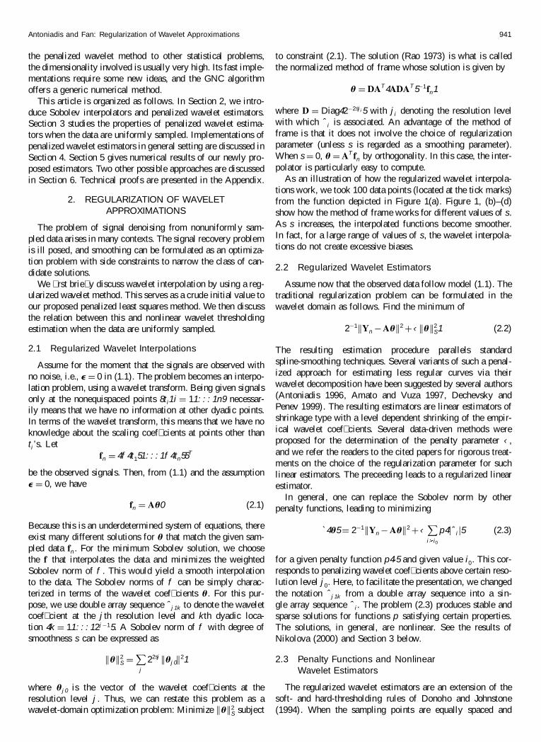
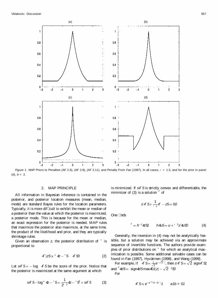