regularization with singular energies martin burger institute for computational and applied...
Post on 20-Dec-2015
213 views
TRANSCRIPT

Regularization with Singular Energies
Martin Burger
Institute for Computational and Applied MathematicsEuropean Institute for Molecular Imaging (EIMI)
Center for Nonlinear Science (CeNoS)
Westfälische Wilhelms-Universität Münster

4.6.2007 Regularization with Singular Energies AIP 2007, Vancouver, June 07
In many inverse and imaging problems, a- priori information on the solution (or its interesting parts) needs to introduced in an effective way, e.g.
- smoothness away from edges (images) - (almost) piecewise constant (material densities with interfaces) - sparsity in some basis / frame (MRI, .. ), or in space (deconvolution, EEG/MEG, ..)
Introduction
¸2kAu ¡ f k2+
12kLuk2 ! min
u

4.6.2007 Regularization with Singular Energies AIP 2007, Vancouver, June 07
Nanoscopy with optical (4pi) techniques, cell imaging: sparsity in space
© Andreas Schönle, MPI Göttingen
Examples
¸2kAu ¡ f k2+
12kLuk2 ! min
u

4.6.2007 Regularization with Singular Energies AIP 2007, Vancouver, June 07
PET / CT imaging of mouse heart coronal sagittal transverse
© Dept of Nuclear Medicine / SFB 658, WWU Münster
Examples
¸2kAu ¡ f k2+
12kLuk2 ! min
u

4.6.2007 Regularization with Singular Energies AIP 2007, Vancouver, June 07
MRI images for EEG/MEG modelling T1 PD
© Institute for BioSystemAnalysis, WWU Münster
Anisotropic Structures essential for field simulations and dipole source reconstructions in MEG
Examples
¸2kAu ¡ f k2+
12kLuk2 ! min
u

4.6.2007 Regularization with Singular Energies AIP 2007, Vancouver, June 07
MRI images for EEG/MEG modelling
Baillet, Mosher, Leahy, IEEE Signal Processing Magazine, 2001, 18(6), pp. 14-30.
Examples
¸2kAu ¡ f k2+
12kLuk2 ! min
u

4.6.2007 Regularization with Singular Energies AIP 2007, Vancouver, June 07
Aerial images of buildings: strong anisotropy
© Aerowest GmbH
Münster Visualization Project, Dept. of Computer Science, WWU
Examples
¸2kAu ¡ f k2+
12kLuk2 ! min
u

4.6.2007 Regularization with Singular Energies AIP 2007, Vancouver, June 07
A-priori information or desired structures have to be incorporated into reconstruction methods and regularization schemes
One possibility are singular energies (not differentiable and not strictly convex), see also various speakers at AIP 07: Daubechies, Candes, Fornasier, Saab, Leitao, Mizera, Kindermann, Lorenz, Ramlau, Rauhut, Zhariy, Ring, Villegas, Klann, …
Introduction
¸2kAu ¡ f k2+
12kLuk2 ! min
u

4.6.2007 Regularization with Singular Energies AIP 2007, Vancouver, June 07
Classical regularization schemes for inverse problems and imaging are based on linear smoothing = quadratic energy functionals
Example: Tikhonov regularization for linear operator equations A u = f
Linear Regularization
¸2kAu ¡ f k2+
12kLuk2 ! min
u
¸2kAu ¡ f k2+
12kLuk2 ! min
u

4.6.2007 Regularization with Singular Energies AIP 2007, Vancouver, June 07
These energy functionals are strictly convex and differentiable – standard tools from analysis and computation (Newton methods etc.) can be used Disadvantage: possible oversmoothing, seen from first-order optimality condition Tikhonov yields
Hence u is in the range of (L*L)-1A*
Linear Tikhonov
¸2kAu ¡ f k2+
12kLuk2 ! min
u
L¤Lu = ¡ ¸A¤(Auf )

4.6.2007 Regularization with Singular Energies AIP 2007, Vancouver, June 07
Classical example: integral equation of the first kind, regularization in L2 (L = Id), A = Fredholm integral operator with kernel k
Smoothness of regularized solution is determined by smoothness of kernel For typical convolution kernels like Gaussians, u is analytic !
Deblurring
¸2kAu ¡ f k2+
12kLuk2 ! min
u
u(x) = ¸Z Z
k(y;x)(¡ k(y;z)u(z) + f (z))dy dz
4.6.2007 Regularization with Singular Energies AIP 2007, Vancouver, June 07
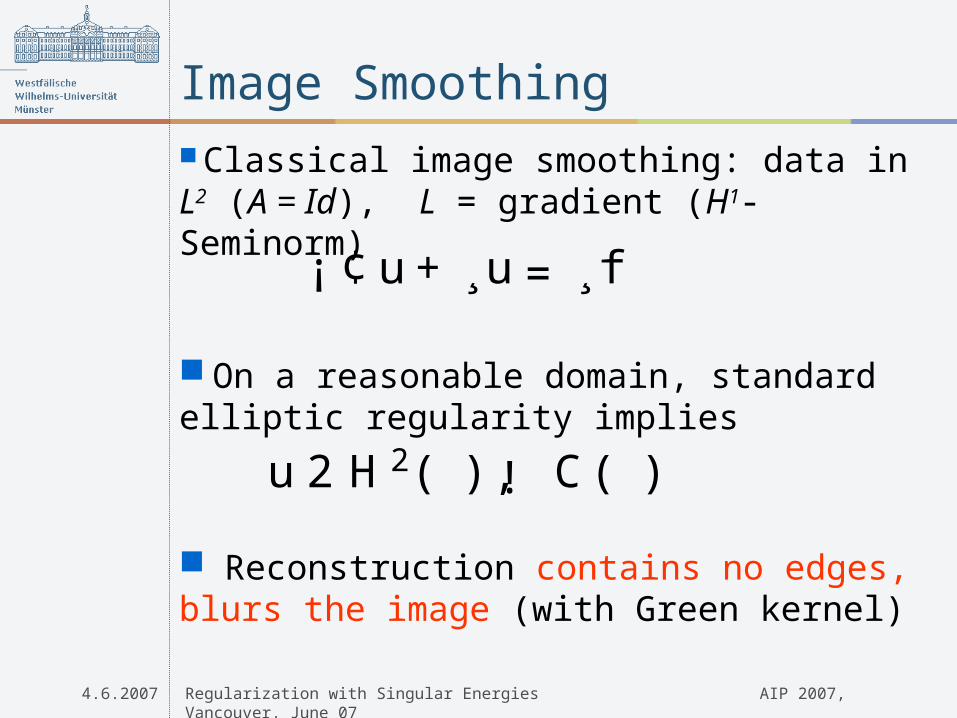
Classical image smoothing: data in L2 (A = Id), L = gradient (H1-Seminorm)
On a reasonable domain, standard elliptic regularity implies
Reconstruction contains no edges, blurs the image (with Green kernel)
Image Smoothing
¸2kAu ¡ f k2+
12kLuk2 ! min
u
¡ ¢ u+¸u = ¸f
u 2 H 2( ) ,! C( )

4.6.2007 Regularization with Singular Energies AIP 2007, Vancouver, June 07
Let A be an operator on (basis repre-sentation of a Hilbert space operator, wavelet)
Penalization by squared norm (L = Id)
Optimality condition for components of u
Decay of components determined by A*. Even if data are generated by sparse signal (finite number of nonzeros), reconstruction is not sparse !
Sparse Reconstructions ?
¸2kAu ¡ f k2+
12kLuk2 ! min
u
2̀(Z)
uk = ¸ (A¤(¡ Au+ f ))k
4.6.2007 Regularization with Singular Energies AIP 2007, Vancouver, June 07
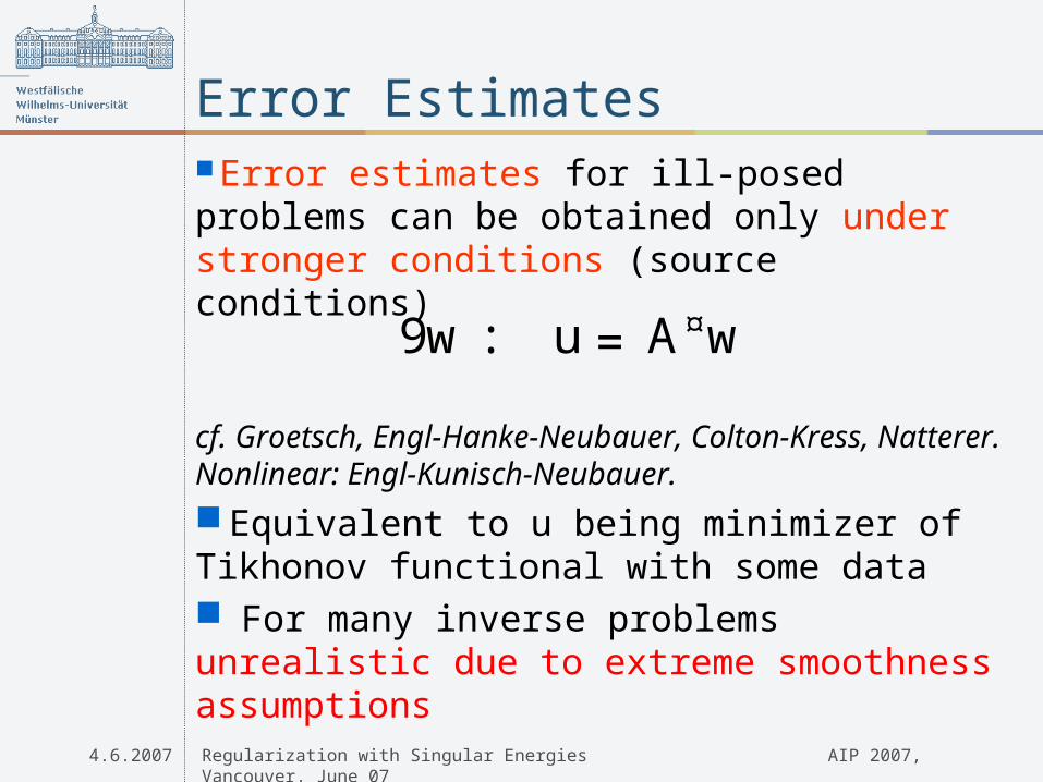
Error estimates for ill-posed problems can be obtained only under stronger conditions (source conditions)
cf. Groetsch, Engl-Hanke-Neubauer, Colton-Kress, Natterer. Nonlinear: Engl-Kunisch-Neubauer.
Equivalent to u being minimizer of Tikhonov functional with some data For many inverse problems unrealistic due to extreme smoothness assumptions
Error Estimates
¸2kAu ¡ f k2+
12kLuk2 ! min
u
9w : u = A¤w

4.6.2007 Regularization with Singular Energies AIP 2007, Vancouver, June 07
Condition can be weakened to
cf. Neubauer et al (algebraic), Hohage (logarithmic), Mathe-Pereverzyev (general).
Advantage: more realistic conditions
Disadvantage: Estimates get worse with
Error Estimates
¸2kAu ¡ f k2+
12kLuk2 ! min
u
9v : u =¾(A¤A)v
4.6.2007 Regularization with Singular Energies AIP 2007, Vancouver, June 07
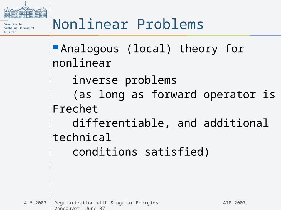
Analogous (local) theory for nonlinear
inverse problems (as long as forward operator is Frechet differentiable, and additional technical conditions satisfied)
Nonlinear Problems
¸2kAu ¡ f k2+
12kLuk2 ! min
u

4.6.2007 Regularization with Singular Energies AIP 2007, Vancouver, June 07
Image smoothing: try nonlinear energy
for penalization:
Optimality condition is nonlinear PDE
r is strictly convex and smooth: usual smoothing behaviour / elliptic regularity
r is not convex: problem not well-posed
Try borderline case: singular energy
Singular Energies
¸2kAu ¡ f k2+
12kLuk2 ! min
u
¡ r ¢((r r)(r u)) +¸u= ¸f
Rr(r u)

4.6.2007 Regularization with Singular Energies AIP 2007, Vancouver, June 07
Simplest choice yields total variation method (Rudin-Osher-Fatemi 89, Acar-Vogel 93, Chambolle-Lions 96, …)
Singular energy: nondifferentiable, not strictly convex
„ “
Total Variation Methodsr(p) = jpj
jujB V =
Zjr uj dx
jujB V = supg2C 10 ;kgk1 · 1
Zu(r ¢g) dx

4.6.2007 Regularization with Singular Energies AIP 2007, Vancouver, June 07
A operator on
Singular energy
Regularized minimization
Daubechies et al 04-07, Loubes 06/07, Ramlau, Maass, Klann 07, …
Sparsity
¸2kAu ¡ f k2+
12kLuk2 ! min
u
2̀(Z) \ 1̀(Z)
J (u) = kuk1 =Pjukj
¸2kAu ¡ f k2+J (u) ! min
u

4.6.2007 Regularization with Singular Energies AIP 2007, Vancouver, June 07
Optimality condition for components of u
A* is the adjoint operator to ,hence
Implies sparsity of u, since
Sparsity
¸2kAu ¡ f k2+
12kLuk2 ! min
u
sign (uk) = ¸A¤(f ¡ Au)k
sign (uk) 2 2̀(Z)
2̀(Z)
ksign(u)k2 =number of nonzero components
4.6.2007 Regularization with Singular Energies AIP 2007, Vancouver, June 07
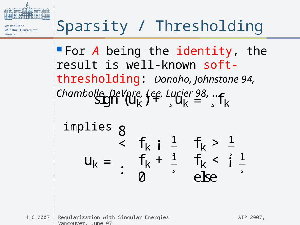
For A being the identity, the result is well-known soft-thresholding: Donoho, Johnstone 94,
Chambolle, DeVore, Lee, Lucier 98, …
implies
Sparsity / Thresholding
¸2kAu ¡ f k2+
12kLuk2 ! min
u
uk =
8<
:
f k ¡ 1¸ f k > 1
¸f k + 1
¸ f k < ¡ 1¸
0 else
sign (uk) +¸uk = ¸f k

4.6.2007 Regularization with Singular Energies AIP 2007, Vancouver, June 07
ROF model for denoising
Rudin-Osher Fatemi 89/92, Chambolle-Lions 96, Scherzer-Dobson 96, Meyer 01,…
ROF Model
¸2
Z(u ¡ f )2+jujB V ! min
u2B V
4.6.2007 Regularization with Singular Energies AIP 2007, Vancouver, June 07
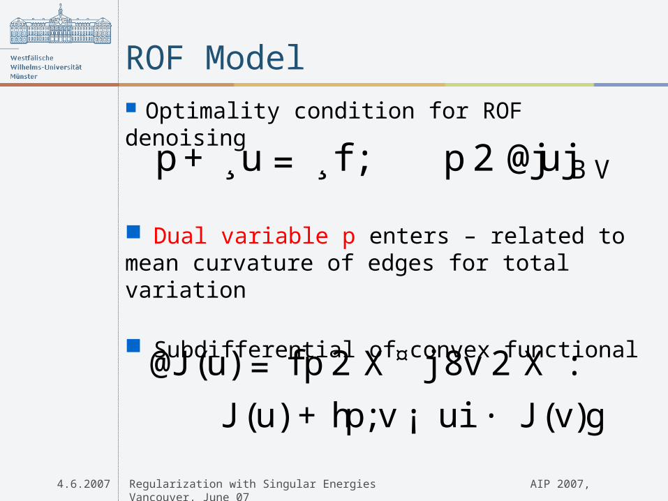
Optimality condition for ROF denoising
Dual variable p enters – related to mean curvature of edges for total variation
Subdifferential of convex functional
ROF Model
p+¸u= ¸f ; p2 @jujB V
@J (u) = fp2 X ¤ j 8v 2 X :
J (u) +hp;v ¡ ui · J (v)g

4.6.2007 Regularization with Singular Energies AIP 2007, Vancouver, June 07
ROF Model
Reconstruction (code by Jinjun Xu)
clean noisy ROF

4.6.2007 Regularization with Singular Energies AIP 2007, Vancouver, June 07
ROF model denoises cartoon images resp. computes the cartoon of an arbitrary image, natural spatial multi-scale decomposition by varying
ROF Model

4.6.2007 Regularization with Singular Energies AIP 2007, Vancouver, June 07
Bachmayr, 2007
Numerical Differentiation with TV
4.6.2007 Regularization with Singular Energies AIP 2007, Vancouver, June 07
Methods with singular energies have great potential, but still some problems:- difficult to analyze and to obtain error estimates- systematic errors (like loss of contrast)- computational challenges- strong bias – how to incorporate uncertain a-priori structures (adaptively) ?
Singular Energies
4.6.2007 Regularization with Singular Energies AIP 2007, Vancouver, June 07
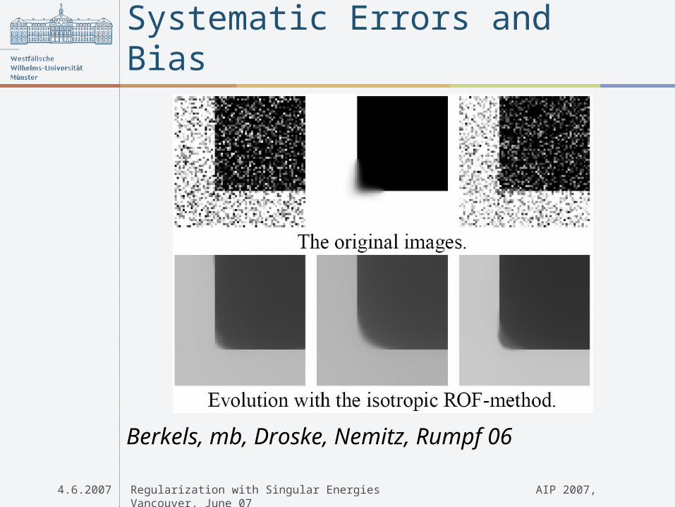
Berkels, mb, Droske, Nemitz, Rumpf 06
Systematic Errors and Bias

4.6.2007 Regularization with Singular Energies AIP 2007, Vancouver, June 07
ROF minimization loses contrast, total variation of the reconstruction is smaller than total variation of clean image. Image features left in residual f-u
g, clean f, noisy u, ROF f-u
mb-Gilboa-Osher-Xu 06
Loss of Contrast

4.6.2007 Regularization with Singular Energies AIP 2007, Vancouver, June 07
Idea: add the residual („noise“) back to the image to pronounce the features decreased too much. Then do ROF again. Iterative procedure
Osher-mb-Goldfarb-Xu-Yin 04
Iterative Refinement
uk =argminu
·¸2
Z(u ¡ f ¡ vk¡ 1)2+jujB V
¸
vk =vk¡ 1+(f ¡ uk); v0 =0

4.6.2007 Regularization with Singular Energies AIP 2007, Vancouver, June 07
Improves reconstructions significantly
Iterative Refinement & ISS

4.6.2007 Regularization with Singular Energies AIP 2007, Vancouver, June 07
Iterative Refinement & ISS

4.6.2007 Regularization with Singular Energies AIP 2007, Vancouver, June 07
Works for inverse problems in a similar way
Osher-mb-Goldfarb-Xu-Yin 04
Iterative Refinement
uk =argminu
·¸2kAu¡ f ¡ vk¡ 1k2+J (u)
¸
vk =vk¡ 1+(f Auk); v0 =0

4.6.2007 Regularization with Singular Energies AIP 2007, Vancouver, June 07
Observation from optimality condition
Implies relation between decomposed residual and subgradient
Iterates determined by equivalent minimization of
Iterative Refinement & ISS
pk = ¸A¤vk
¸2kAu¡ f k2+J (u) J (uk¡ 1) ¡ ¸hvk¡ 1;Au Auk¡ 1i
=¸2kAu¡ f k2+J (u) J (uk¡ 1) ¡ hpk¡ 1;u uk¡ 1i
pk = ¸A¤(¡ Auk +f +vk¡ 1) 2 @J (uk)

4.6.2007 Regularization with Singular Energies AIP 2007, Vancouver, June 07
Dual update formula
Iterative refinement = dual proximal method = Bregman iteration. Minimization in each step of
Generalized Bregman distance
Iterative Refinement & ISS
¸2kAu¡ f k2+Dpk ¡ 1J (u;uk¡ 1)
DqJ (u;v) = J (u) J (v) ¡ hq;u viq2 @J (v)
pk =pk¡ 1+¸A¤(¡ Auk +f )

4.6.2007 Regularization with Singular Energies AIP 2007, Vancouver, June 07
Choice of parameter less important, can be kept small (oversmoothing). Regularizing effect comes from appropriate stopping.
Quantitative stopping rules available, or „stop when you are happy“ in imaging – S.O. Limit to zero can be studied. Yields gradient flow for the dual variable („inverse scale space“)
mb-Gilboa-Osher-Xu 06, mb-Frick-Osher-Scherzer 06
Iterative Refinement & ISS
@tp(t) = A¤(¡ Au(t) + f ); p2 @J (u)

4.6.2007 Regularization with Singular Energies AIP 2007, Vancouver, June 07
Efficient numerical schemes for flow mb-Gilboa-Osher-Xu 06
Analysis of iteration and partly of the flowOsher-mb-Goldfarb-Xu-Yin 04, mb-Frick-Osher-Scherzer 06
Error estimates in Bregman distance mb-He-Resmerita 07
Non-quadratic fidelity is possible, some caution needed for L1 fidelityHe-mb-Osher 05, mb-Frick-Osher-Scherzer 06
Iterative Refinement & ISS
4.6.2007 Regularization with Singular Energies AIP 2007, Vancouver, June 07
Application to other energies, e.g. Besov norms (wavelets), is straight-forward
Starting from soft shrinkage, iterated refinement yields firm shrinkage, inverse scale space becomes hard shrinkageOsher-Xu 06
Bregman is distance natural sparsity measure, number of nonzero components is constant in error estimates
Iterative Refinement & ISS

4.6.2007 Regularization with Singular Energies AIP 2007, Vancouver, June 07
Smoothing of surfaces in level set represenation
3D Ultrasound, Kretz / GE Med.
Surface Smoothing
4.6.2007 Regularization with Singular Energies AIP 2007, Vancouver, June 07
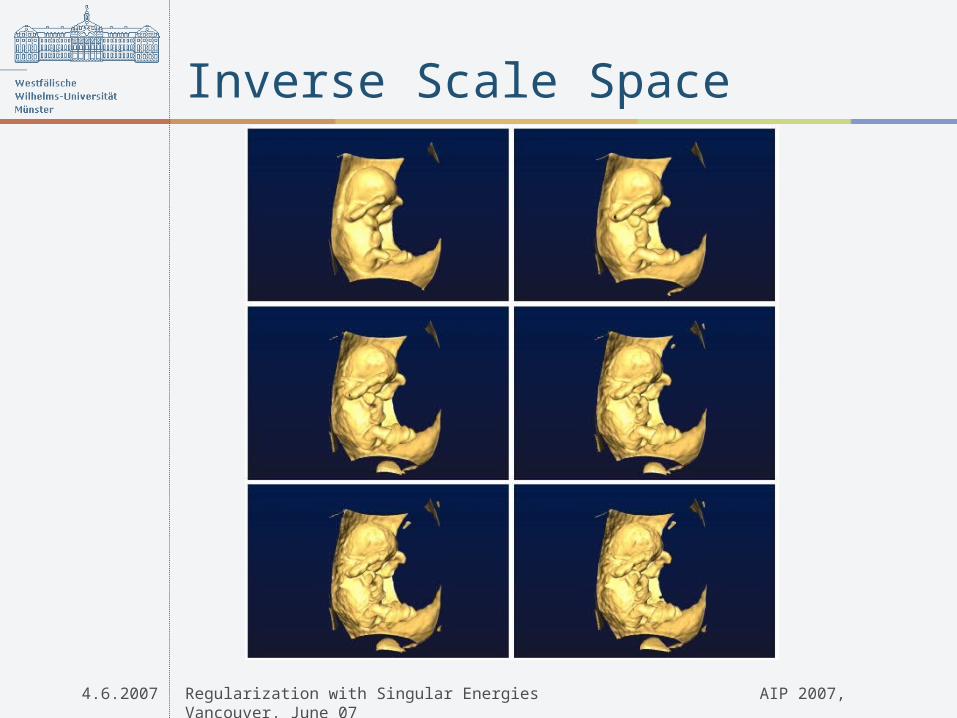
Inverse Scale Space

4.6.2007 Regularization with Singular Energies AIP 2007, Vancouver, June 07
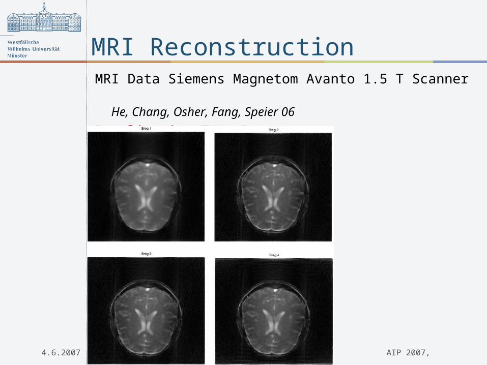
MRI Data Siemens Magnetom Avanto 1.5 T Scanner He, Chang, Osher, Fang, Speier 06
Penalization TV + Besov
MRI Reconstruction
4.6.2007 Regularization with Singular Energies AIP 2007, Vancouver, June 07
MRI Data Siemens Magnetom Avanto 1.5 T Scanner He, Chang, Osher, Fang, Speier 06
Penalization TV + Besov
MRI Reconstruction

4.6.2007 Regularization with Singular Energies AIP 2007, Vancouver, June 07
Generalization to nonlinear inverse problems possible Bachmayr, Thesis 07
Different ways of approximating nonlinearity lead to different iterative schemes (similar to iterated Tikhonov / Landweber / Levenberg-Marquardt)
Example: parameter identification (diffusivity) in elliptic PDE
Iterative Refinement & ISS

4.6.2007 Regularization with Singular Energies AIP 2007, Vancouver, June 07
Exact Solution
Reconstructions at 1 % noise
Iterative 1 Iterative 2 Standard TV
Iterative Refinement & ISS
4.6.2007 Regularization with Singular Energies AIP 2007, Vancouver, June 07
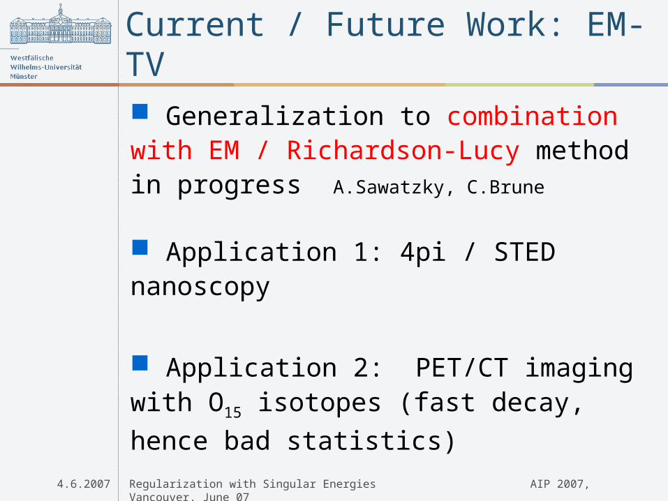
Generalization to combination with EM / Richardson-Lucy method in progress A.Sawatzky, C.Brune
Application 1: 4pi / STED nanoscopy
Application 2: PET/CT imaging with O15
isotopes (fast decay, hence bad statistics)
Current / Future Work: EM-TV

4.6.2007 Regularization with Singular Energies AIP 2007, Vancouver, June 07
Bias of one functional often too strong
Better: use a family of functionals parametrized by
Example: adaptive anisotropy in total variation methods
Adaptive Bias / Parametrization
J (u;®)®2 A

4.6.2007 Regularization with Singular Energies AIP 2007, Vancouver, June 07
In aerial images the typical anisotropy is rectangular, houses have 90° angles
But not all of them have the same orientation
Adaptive Anisotropy

4.6.2007 Regularization with Singular Energies AIP 2007, Vancouver, June 07
Bias for edges with 90° angles from functional of the form
R is rotation matrix for angle to capture
the orientation
Since orientation is not constant over the image, has to vary and to be found adaptively by minimization
Adaptive Anisotropy
J (u;®) =
Z(jv1j + jv2j) dx; v=R®r u
4.6.2007 Regularization with Singular Energies AIP 2007, Vancouver, June 07
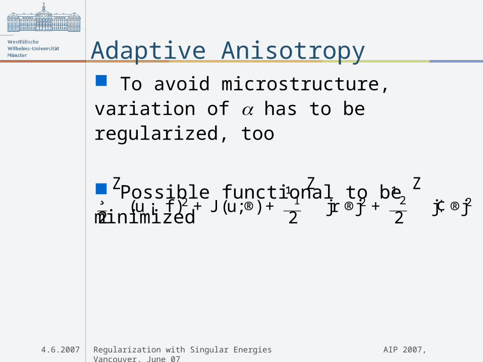
To avoid microstructure, variation of has to be regularized, too
Possible functional to be minimized
Adaptive Anisotropy
¸2
Z(u ¡ f )2+J (u;®) +
¹ 12
Zjr ®j2+
¹ 22
Zj¢®j2
4.6.2007 Regularization with Singular Energies AIP 2007, Vancouver, June 07
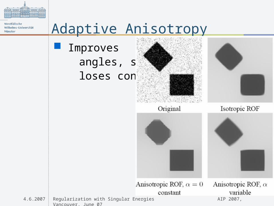
Improves angles, still loses contrast
Adaptive Anisotropy

4.6.2007 Regularization with Singular Energies AIP 2007, Vancouver, June 07
Contrast correction again by iterative refinement
Angle parameter provides classification of orientations in the image
Adaptive Anisotropy

4.6.2007 Regularization with Singular Energies AIP 2007, Vancouver, June 07
Cartoon reconstruction and orientational classification of aerial images
Berkels, mb, Droske, Nemitz, Rumpf 06
Adaptive Anisotropy

4.6.2007 Regularization with Singular Energies AIP 2007, Vancouver, June 07
Cartoon reconstruction and orientational classification of aerial images
Berkels, mb, Droske, Nemitz, Rumpf 06
Adaptive Anisotropy

4.6.2007 Regularization with Singular Energies AIP 2007, Vancouver, June 07
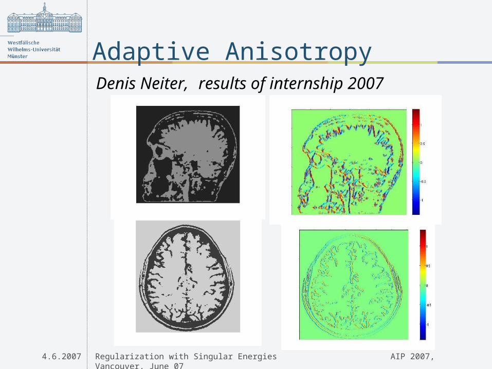
Analogous problem in segmentation of MRI brain images for EEG/MEG
Regularization by total variation (= length of curves in segmentation) kills noise, but also elongated structures
Adapt anisotropy (locally like sharp ellipse) to find sulci accurately and provide classification of normals (for dipole fitting, source reconstruction)
Adaptive Anisotropy
4.6.2007 Regularization with Singular Energies AIP 2007, Vancouver, June 07
Denis Neiter, results of internship 2007
Adaptive Anisotropy

4.6.2007 Regularization with Singular Energies AIP 2007, Vancouver, June 07
Papers and talks at
www.math.uni-muenster.de/u/burgeror by email
Thanks for input and suggestions to:
S.Osher, J.Xu, G.Gilboa, D.Goldfarb, W.Yin, L.He, E.Resmerita, M.Bachmayr, B.Berkels, M.Droske, O.Nemitz, M.Rumpf, K.Frick, O.Scherzer, A.Schönle, T.Hohage, C.Wolters, T.Kösters, K.Schäfers, F.Wübbeling, A.Sawatzky, D.Neiter
Download and Contact