regularized laplacian zero crossings as optimal edge...

Regularized Laplacian Zero Crossings as Optimal Edge Integrators

R. KIMMEL A.M. BRUCKSTEIN

Department of Computer Science

Technion–Israel Institute of Technology

Technion City, Haifa 32000, Israel

Abstract

We view the fundamental edge integration problem for object segmentation in a geometric vari-ational framework. First we show that the classical zero-crossings of the image Laplacian edgedetector as suggested by Marr and Hildreth, inherently provides optimal edge-integration with re-gard to a very natural geometric functional. This functional accumulates the inner product betweenthe normal to the edge and the gray level image-gradient along the edge. We use this observation toderive new and highly accurate active contours based on this functional and regularized by previouslyproposed geodesic active contour geometric variational models.

1. Introduction

Edge integration for segmentation is an old, yet still very active area of research in low-level image

analysis. Textbooks in computer vision treat edge detection and edge integration as separate topics, the

first being considered one of labelling edges in the image to be followed by a process of integrating

the local “edges” into meaningful curves. In fact one may view basic edge detection as a process of

estimating the gradient of the image, i.e. computing at each pixel��

the values ��and � � ��

by using the values of � � ��over a neighborhood � � ��

of� ��

and designating as edges the places

where the length of the gradient vector estimate �� exceeds some threshold value.

The more advanced edge detectors such as those proposed by Marr and Hildreth [7] attempt to locate

points or curves defined by local maxima of the image gradient. The Marr Hildreth proposal for edge

1

Tec

hnio

n - C

ompu

ter S

cien

ce D

epar

tmen

t - T

echn

ical

Rep

ort

CIS

-200

1-04

- 20

01

detection yields curves that delineate the zero crossing of the Laplacian operator applied to a smoothed

version of the image input. The smoothing proposed is via a Gaussian convolution operator and its width

is a parameter that can be varied providing the opportunity to do scale space processing and “vertical”

integration on the zero-crossing curves.

In this paper we propose to regard the edge detection and integration process as a way to determine

curves in the image plane that pass through points where the gradient is high and whose direction best

corresponds to the local edge direction predicted by the estimated gradient.

Indeed, if we somehow estimate the gradient field �� based on considering � ��for

each pixel� ��

over some neighborhood �� , where � is a size parameter, we shall have at each

point a value, given by the intensity of the gradient� � �� "!# , that tells us how likely

an edge is at this point and, if an edge exists, its likely direction will be perpendicular to the vector�� . It is therefore natural to look for curves in the image plane, $ ��%"� �&� �� %"��%'� � , that

pass through points with high intensity gradients with tangents agreeing as much as possible to the edge

directions there. Thus we are led to consider the following functional, evaluating the quality of $ ��%'�as

an edge-curve candidate,(*) � $ � %"�+� � ,.-/10324 �� $ ��%'�+�� $ � %"� � �"5768:9 ;< ; 9=>@?BA $ � %"�A % CED�FG A %

where 0 � 5 � is some monotonically increasing function. Here, the inner product of� �H�I�� J� with the

normal to $ � %"�, given by KL � %"� � 68 9 ;< ; 9

=> ?MA $ ��%'�A % C�D �where $ ��%"�

is an arclength parameterized curve, is a measure of how well $ � %"�is locally tracking an

edge. Indeed we want $ ��%'�to pass at high gradient locations in the edge direction, and hence the inner

product of its normal with the estimated gradient of � should be high, indicating both alignment and

considerable change in image intensity there. This inner product will also be proportional to the gradient

magnitude, since �� $ ��%"� �� $ � %"�+� � 68 9 ;< ; 9=> ? A $A % C D �ON � �PNQ5SRUT'V � W��

2

Tec

hnio

n - C

ompu

ter S

cien

ce D

epar

tmen

t - T

echn

ical

Rep

ort

CIS

-200

1-04

- 20

01

whereW

is the angle between the outward pointing normal

KL to $ � %"�and the gradient direction.

The functionals(X)

measure how well an arclength parameterized curve of length Y approximates an

edge in the image plane. Our task, of course is to determine several most probable edge curves in the

image plane. We shall do so by determining curves that locally maximize these functionals.

Suppose first that we are considering closed contours $ � %"�, and that 0 ��ZX� � Z

. Then, we have that( � $ ��%'�+� �\[^]E_a`cbedf � $ ��%"� � AA % ��%'� < � � $ ��%'�+� AA % ��%'��g A %��and Green’s theorem yields( � $ ��%'�+� � ,e,.h�i dkjj � � � ��E� jj � � �� g A � A �E�where l ]

is the region inside $ � %"�. But, recalling that � � ��

is an estimate of mmon � � ��and ��

an

estimate of mmop � � ��we have( � $ ��%'�+�rq� ,e, h�i d j �j � � � � ��f� j �j � � � � �� g A � A �q� ,e,.h�i ��s � � �� A � A ��t

Therefore, the functional that we want to maximize is the integrated Laplacian over the area enclosed by$ � %"�. This means that if we have an area where the Laplacian is positive

( � $ � %"� �should expand from

within this area to the places wheres � � ��

becomes zero and subsequently changes sign. This shows

that optimal edge-curves in the sense of maximizing( � $ � %"� �

are the zero crossings of the Laplacian.

If we initialize $ � %"�as a small circular “bubble” at a place where

s � � ��is positive and then let$ � %"�

evolve according to a rule that implements a gradient descent in conjunction with the functional( � $ � %"� ��i.e. we implement AA"u $ � %�� u � �Iv ( � $ � %�w u � �v $ �

the curve $ � %�� u �will expand in time

uto the nearest zero-crossing curve of the input image Laplacian.

Therefore, we have obtained a beautiful interpretation of the classical Marr-Hildreth edge detection

method [7]. The zero-crossings of the Laplacian are curves that best integrate the edges, in the sense

of our functional(X) � $ � %"� �

with 0 ��ZX� � Z, if we wish to do so based on gradients estimated for the

(smoothed) input image � � ��. While this fact is pedagogically very pleasing, it does not alleviate the

3

Tec

hnio

n - C

ompu

ter S

cien

ce D

epar

tmen

t - T

echn

ical

Rep

ort

CIS

-200

1-04

- 20

01

notorious over sensitivity properties of this edge-detector which in noisy images yields lots of false edge

curves. However, we shall show here that this insight provides the basis for a new and practical active

contour process which enhances and improves upon the previously designed such methods for image

segmentation.

We next present the full derivation of the variational results leading to the new edge integration pro-

cesses and then show the performance of the resulting algorithms.

2. Closed Active Contours: Derivation

Motivated by the classical ‘snakes’ [4], geometric active contours [5, 1], and finally the ‘geodesic active

contours’ that were shown in [2] to be related to the ‘snakes’, we search for simple parametric curves

in the plane that map their arclength interval � 9 � Yx� to the plane, such that $zy{� 9 � Yx�7| IR � , or in an

explicit parametric form $ ��%"� �}� ��%'��E� %"� � . Here%

is the arclength parameter, and we have the relation

between the arclength%

and a general arbitrary parameterization ~ , given byA % � d A �� ~ �A ~ g � � d A �E� ~ �A ~ g � A ~��ON�$*�^N A ~ tWe define, as usual,

KL ��and

Kuto be the unit normal, the curvature, and the tangent of the curve $ .

We have that� KL �\$ `c`

, and

Ku ��$ ` �\$ �S� N�$ � N . As described in the introduction, consider the geometric

functional (�) � $ � �\[ -/10 �+�K� � KL� � A %�t

This is an integration along the curve $ of a function 0 defined in terms of a vector field

K� �� ,where for example we can take

K� � � � �� p � � n � as the gray level image gradient. Our goal is to

find curves $ that minimize the above geometric functional.

In a general parametric form, we have the following re-parameterization invariant measure(*) � $ � �\[��/�0 �+�K� � KL� � N�$*�^N A ~ t

Define,Z��r� K� � KL� . The Euler Lagrange (EL) equations v ( ) � $ � � v $�� 9 should hold along the ex-

4

Tec

hnio

n - C

ompu

ter S

cien

ce D

epar

tmen

t - T

echn

ical

Rep

ort

CIS

-200

1-04

- 20

01

tremum curves, and for a closed curve these equations arev (�) � $ �v $ � 24 mmop <�� mm�p �mmon <z�� mm�n � FG 0 � Z*� N�$*�^N �or in a more compact form v (�) � $ �v $ ��d@jj $ < AA ~ jj $ � g 0 � Z*� N�$ � N �where we use the shorthand notation j � j $\�� j � j �� j � j � � D and j � j $*�� j � j � � � j � j � �� D . In case of

an open curve, one must also consider the end points and add additional constraints to determine their

optimal locations.

Before we work out the general 0 � Z*�case let us return to the simple example discussed in the intro-

duction, where 0 � Z*� � Z. In this case we have that( � $ � � [��/ � K� � KL� N�$*�^N A ~� [��/O�

K� � � < � � �� N�$*�^N � N�$*�'N A ~� [��/ � < � �B �� M� � A ~ tThe EL equation for the

�part is given byv (v � � d jj � < AA ~ jj � � g � < � � �.� � � �� < � � p �� p < AA ~ �� < � �B p �� B� p < � p � � < � n � �� < � � � p � � n � � < � �B�^�� K� ��t

In a similar way, the�

part of the EL equations is given byv (v � � dkjj � < AA ~ jj � � g.� < � � �.� � � �� < � �B n �.� �B� n � AA ~ � < � �B n �.� �B� n � p � � � n � �� p � � n � � � �B�� K� ��t5

Tec

hnio

n - C

ompu

ter S

cien

ce D

epar

tmen

t - T

echn

ical

Rep

ort

CIS

-200

1-04

- 20

01

Since the EL equations are derived with respect to a geometric measure, we can use the freedom of

reparameterization for the curve $ , divide by N�$��^N , and obtain the “geometric EL equation:” v ( � v $@��^�� K� � KL , and for

K� � � � � ��we have v ( � v $\� s � KL , where

s � � � p�p � � n�n is the usual Laplacian

operator. It is obvious from this that the geometric EL condition is satisfied along the zero crossing

curves of the image Laplacian, which as described above explains the Marr-Hildreth [7, 6] edge detec-

tor from a global-variational point of view. Below, we shall extract further insights and segmentation

schemes from this observation. We note that heuristic non-variational flows on vector fields were pre-

sented in [13, 10]. In a recent related result, introduced by Vasilevskiy and Siddiqi [12], alignment with

a vector field is used as a minimization criteria for segmentation of complicated closed thin structures in

3D medical images.

As a second example we consider 0 � Z*� ��N Z NJ�@� Z � . The EL is given byv (v $ � � K� � KL�N � K� � KL� N �^�� K� � KL� V�� "¡ �+� K� � KL�� K� � KL �

and for

K� � � � we have v ( � v $¢��V�� "¡ � � � � � KLf� ��s � KL . The new term V£�� "¡ � �� KL¤� � , allows the model

to automatically handle changing contrasts between the objects and the background. For example, it

handles equally well an image of dark objects on bright background and the negative of this image.

Now, we are ready to pursue the general case for 0 ��ZX�in the functional

(�) � $ �(where

Z � � K� � KL� ).We shall use often the following readily verified relationships,AA ~ � N�$ � N AA %j N�$ � Nj $*� � KuA KLA % � < � KuA KuA % � � KLA 0 � Z*�A % � 0�¥ Z ` � � � 0 �

Ku �A ZA % � � K� ` � KL� �¦� K� � KL ` � � � K� ` � KL� < �� K� � Ku �j Zj $*� � < N�$ � N�§ � �K� � Ku � KL �

6

Tec

hnio

n - C

ompu

ter S

cien

ce D

epar

tmen

t - T

echn

ical

Rep

ort

CIS

-200

1-04

- 20

01

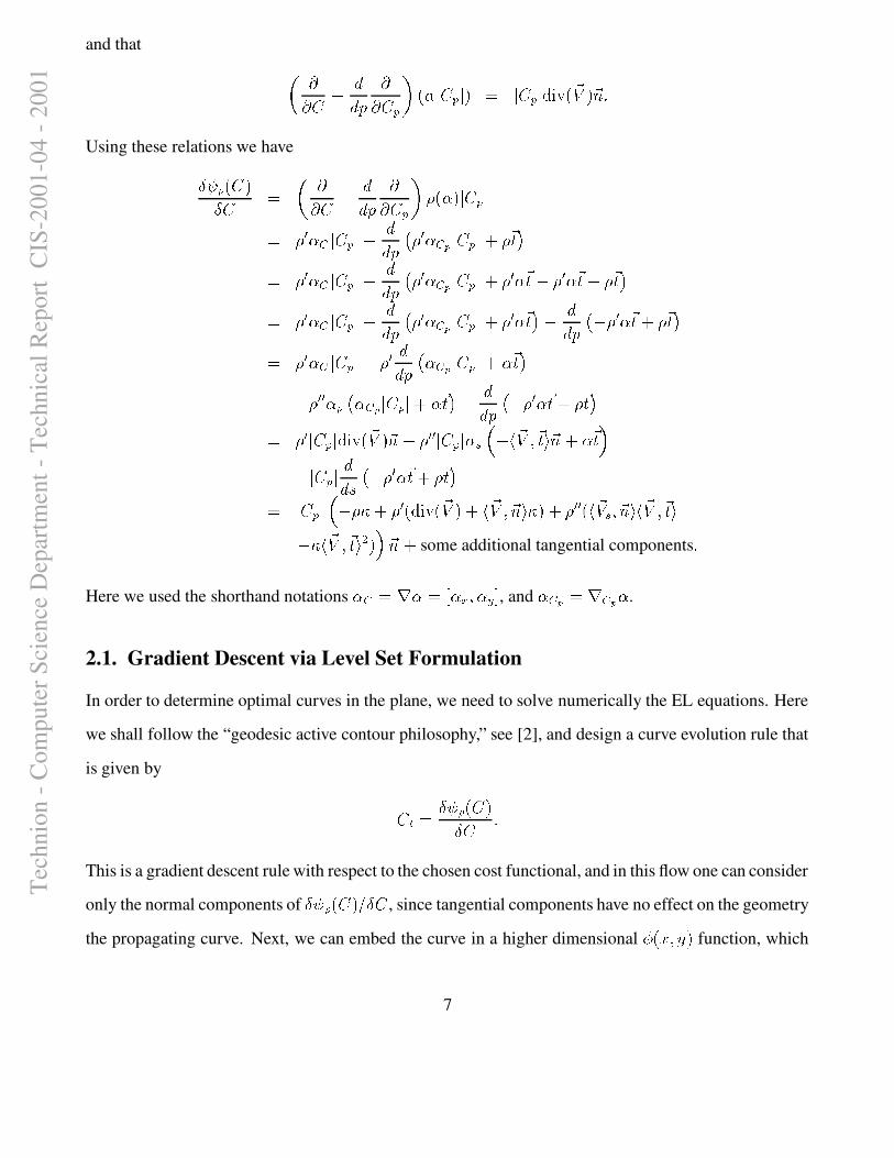
and that d jj $ < AA ~ jj $*� g.� Z N�$*�^N � � N�$*�'N¨�� K� � KL tUsing these relations we havev ( ) � $ �v $ � d jj $ < AA ~ jj $*� g 0 � Z*� N�$*�^N� 0 ¥ Z ] N�$ � N < AA ~3© 0 ¥ Z ] � N�$ � N � 0

Ku�ª� 0 ¥ Z ] N�$*�'N < AA ~ © 0 ¥ Z ] � N�$*�^N � 0 ¥ Z

Ku < 0 ¥ ZKu � 0

Ku ª� 0�¥ Z ] N�$*�'N < AA ~ © 0�¥ Z ] � N�$*�^N � 0�¥ Z

Ku ª < AA ~ © < 0�¥ ZKu � 0

Ku ª� 0 ¥ Z ] N�$*�'N < 0 ¥ AA ~3© Z ] � N�$*�^N �.Z Ku ª< 0 ¥¨¥ Z � © Z ] � N�$ � N ��Z Ku ª < AA ~ © < 0 ¥ Z

Ku � 0Ku ª� 0�¥ N�$ � N¨�� K� � KL < 0�¥¨¥ N�$ � N Z `¬« < � K� � Ku � KL ��Z Ku�< N�$ � N AA % © < 0 ¥ Z

Ku � 0Ku ª� N�$*�^N « < 0 �®� 0�¥ � �� K� �� K� � KL�� f�� 0�¥¨¥ � �

K� ` � KL�� K� � Ku �< �� K� � Ku � � � KL �some additional tangential components

tHere we used the shorthand notations

Z ] � ��Z �@� Z p ��Z n � , andZ ] � � � ] � Z .

2.1. Gradient Descent via Level Set Formulation

In order to determine optimal curves in the plane, we need to solve numerically the EL equations. Here

we shall follow the “geodesic active contour philosophy,” see [2], and design a curve evolution rule that

is given by $e¯� v (�) � $ �v $ tThis is a gradient descent rule with respect to the chosen cost functional, and in this flow one can consider

only the normal components of v (e) � $ � � v $ , since tangential components have no effect on the geometry

the propagating curve. Next, we can embed the curve in a higher dimensional ° ��function, which

7

Tec

hnio

n - C

ompu

ter S

cien

ce D

epar

tmen

t - T

echn

ical

Rep

ort

CIS

-200

1-04

- 20

01

implicitly represents the curve $ as a zero set, i.e., $±�&²³� �� ´yx° �� 9Jµ . In this way, the well

known Osher-Sethian [8, 11] level-set method can be employed to implement the propagation.

Given the curve evolution equation $ ¯ ��¶ KL , its implicit level set evolution equation reads° ¯ ��¶eN � °eN tThe equivalence of these two evolutions can be easily verified using the chain rule and the relationKL � � ° � N � °eN , ° ¯ � �� ° � $ ¯ � � � � ° � ¶ KL�� ¶ � � ° � � °N � °¬N � �¦¶¬N � °¬N tWe readily have that Ku � ·� °N � °¬N � � < ° n � ° p �N � °eN� � �^��d � °N � °eN gK� ` � �� ` � � ` �f�� Ku � �Q�� Ku � �V�� "¡ � � K� � KL�� V�� ¸¡ � � K� �� ° � ��tThereby, the explicit curve evolution as a gradient descent flow for 0 � Z*� ��N Z N is given by$ ¯ �¹V£�� "¡ �+� K� � KL� ��s � KL �for which the implicit level set evolution is given by° ¯ �¹V£�� "¡ �+� K� �� ° � ��s �fN � °¬N t3. Open Active Contours for Optimal Edge Integration

3.1. The Fua-Leclerc Geometric Model

Fua and Leclerc in [3], were first to propose a geometric model for motion of open curves in the image

to optimize an “edge” finding functional. We shall first describe the Fua-Leclerc functional and then

replace the “geodesic active contour” part of it with our new edge integration quality measure. LetY � $ � � , �/ N�$*��N A ~ �8

Tec

hnio

n - C

ompu

ter S

cien

ce D

epar

tmen

t - T

echn

ical

Rep

ort

CIS

-200

1-04

- 20

01

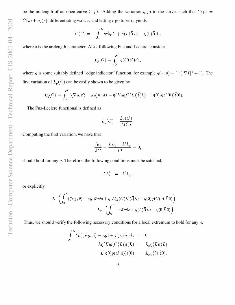
be the arclength of an open curve $ � ~ � . Adding the variation º � ~ � to the curve, such that »$ � ~ � �$ � ~ ��½¼ º � ~ � , differentiating w.r.t.¼, and letting

¼go to zero, yieldsY ¥ � $ � � < ,.-/ � KL º A %�� º � Y � Ku � Y � < º � 9 �

Ku � 9 ��where

%is the arclength parameter. Also, following Fua and Leclerc, considerY¾ � $ � � ,.-/1¿ � $ � %"� � A %J�

where ¿ is some suitably defined “edge indicator” function, for example ¿ � �� ; � � N � �fNÀ� � ; � . The

first variation of Yx¾ � $ �can be easily shown to be given byY ¥¾ � $ � � ,.-/ � � � ¿ �

KL�� < � ¿ �KL º A %�� º � Y � ¿ � $ � Y � � Ku � Y � < º � 9 � ¿ � $ � 9 � �

Ku � 9 ��tThe Fua-Leclerc functional is defined as ( ¾ � $ � � Y¾ � $ �Y � $ � t

Computing the first variation, we have thatv ( ¾v $ � Y¬Y ¥¾ < Y ¥ Y¾Y � � 9 �should hold for any º . Therefore, the following conditions must be satisfied,YeY ¥¾ � Y ¥ Y¾ �or explicitly, Á�Â�Ã^Ä -/¹Å ÆcÇ�ÈEÉ¸ÊË�ÌfÍÏÎ ÈJÐ"ÊË^Ñ�Ò"ÓxÔÕÑ Å Á ÐÖÈ�ÅØ×ÙÅ Á Ð�Ð ÊÚ Å Á Ð Í�Ñ ÅÜÛSÐÖÈPÅ�×ÙÅÝÛSÐ�Ð ÊÚ ÅÝÛSÐ Þß Á ¾ Â Ã^Ä -/ ÍeÎ ÊËEÑ�Ò"ÓxÔÕÑ Å Á Ð ÊÚ Å Á Ð ÍàÑ ÅÜÛSÐ ÊÚ ÅÜÛSÐ ÞÏáThus, we should verify the following necessary conditions for a local extremum to hold for any º ,,.-/ � Y � �� ¿ �

KL�� < � ¿ �x� Y¾ �f� KL º A % � 9Y�º � Y � ¿ � $ � Y �+� Ku � Y � � Y¾âº � Y � Ku � Y �Y�º � 9 � ¿ � $ � 9 � �Ku � 9 � � Y¾âº � 9 �

Ku � 9 ��t9

Tec

hnio

n - C

ompu

ter S

cien

ce D

epar

tmen

t - T

echn

ical

Rep

ort

CIS

-200

1-04

- 20

01

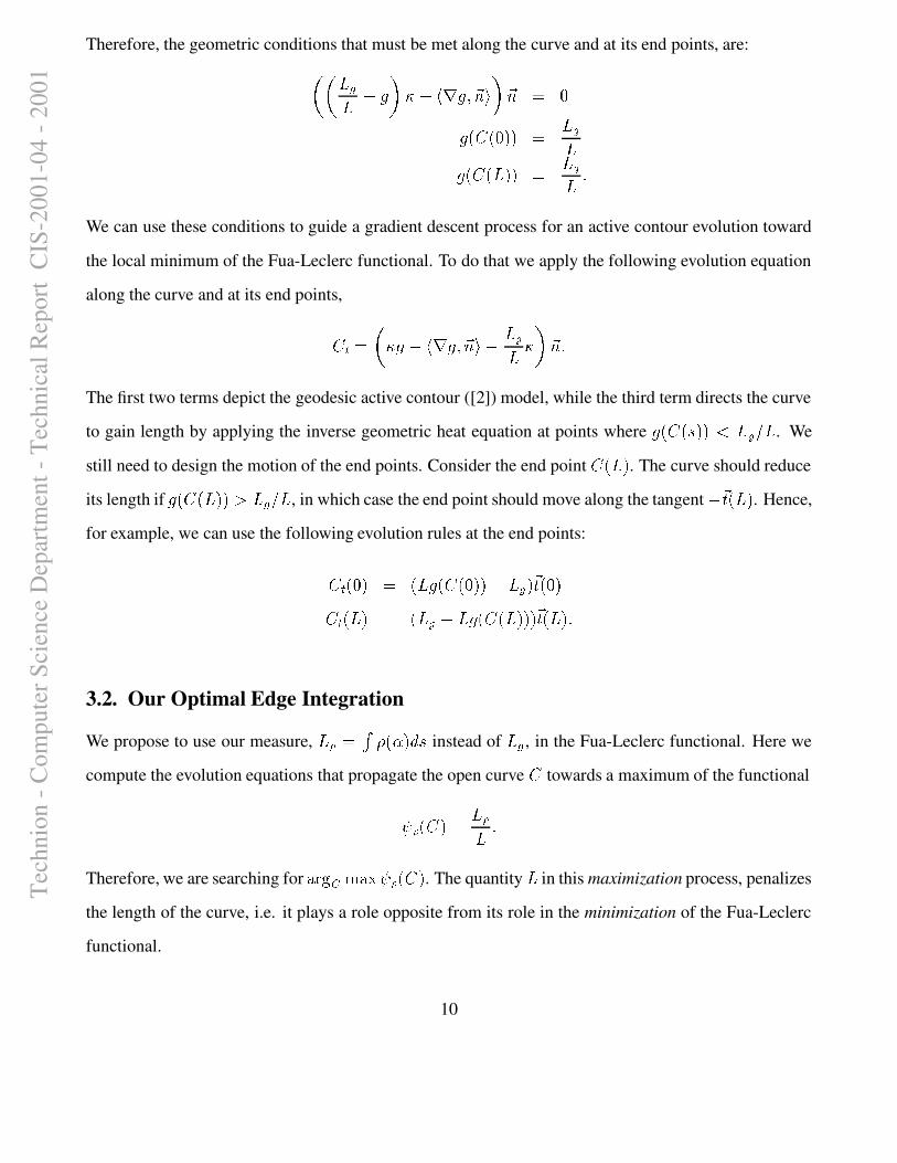
Therefore, the geometric conditions that must be met along the curve and at its end points, are:d7d Y�¾Y < ¿ gã�ä�� ¿ �KL� g KL � 9¿ � $ � 9 � � � Y¾Y¿ � $ � Y �+� � Y¾Y t

We can use these conditions to guide a gradient descent process for an active contour evolution toward

the local minimum of the Fua-Leclerc functional. To do that we apply the following evolution equation

along the curve and at its end points,$ ¯ ��d � ¿ < � � ¿ �KL�� < Y¾Y ��g KL t

The first two terms depict the geodesic active contour ([2]) model, while the third term directs the curve

to gain length by applying the inverse geometric heat equation at points where ¿ � $ ��%'�+�æå Ye¾ � Y . We

still need to design the motion of the end points. Consider the end point $ � Y �. The curve should reduce

its length if ¿ � $ � Y � ��ç Y�¾ � Y , in which case the end point should move along the tangent < Ku � Y �. Hence,

for example, we can use the following evolution rules at the end points:$e¯ � 9 � � � Y ¿ � $ � 9 �+� < Y ¾ � Ku � 9 �$ ¯ � Y � � � Y¾ < Y ¿ � $ � Y �+� � Ku � Y ��t3.2. Our Optimal Edge Integration

We propose to use our measure, Y ) �Oè 0 � Z*� A %instead of Y�¾ , in the Fua-Leclerc functional. Here we

compute the evolution equations that propagate the open curve $ towards a maximum of the functional( ) � $ � � Y )Y tTherefore, we are searching for éSê ]ìë éîí (*) � $ �

. The quantity Y in this maximization process, penalizes

the length of the curve, i.e. it plays a role opposite from its role in the minimization of the Fua-Leclerc

functional.

10

Tec

hnio

n - C

ompu

ter S

cien

ce D

epar

tmen

t - T

echn

ical

Rep

ort

CIS

-200

1-04

- 20

01

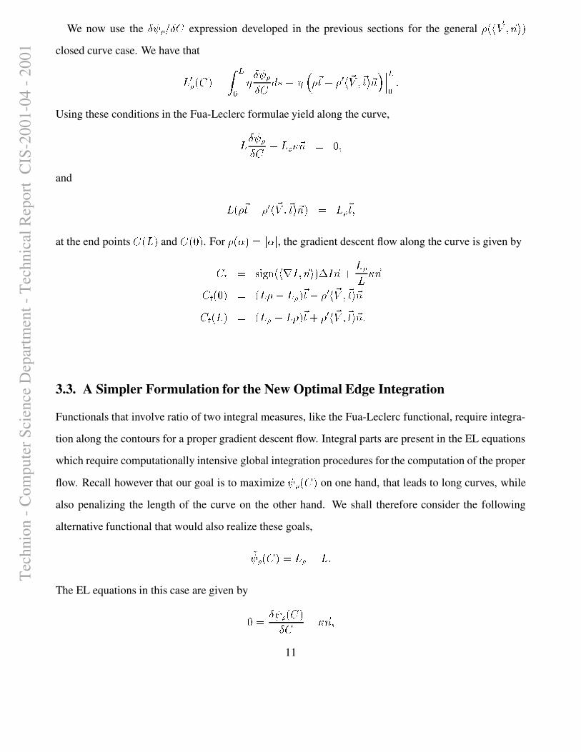
We now use the v (X) � v $ expression developed in the previous sections for the general 0 � �K� � KL� �

closed curve case. We have thatY ¥ ) � $ � � ,.-/ º v (*)v $ A %ï� º « 0Ku < 0 ¥ �

K� � Ku � KL {ððð -/ tUsing these conditions in the Fua-Leclerc formulae yield along the curve,Y v (*)v $ � Y ) � KL � 9 �and Y � 0

Ku < 0 ¥ �K� � Ku � KL � � Y ) Ku �

at the end points $ � Y �and $ � 9 � . For 0 ��ZX� �ON Z N , the gradient descent flow along the curve is given by$e¯±� V�� ¸¡ � �� KL¤� ��s � KL � Y )Y � KL$ ¯ � 9 � � � Y 0 < Y ) � Ku < 0�¥ �

K� � Ku � KL$ ¯ � Y � � � Y ) < Y 0 �Ku � 0 ¥ �

K� � Ku � KL t3.3. A Simpler Formulation for the New Optimal Edge Integration

Functionals that involve ratio of two integral measures, like the Fua-Leclerc functional, require integra-

tion along the contours for a proper gradient descent flow. Integral parts are present in the EL equations

which require computationally intensive global integration procedures for the computation of the proper

flow. Recall however that our goal is to maximize(�) � $ �

on one hand, that leads to long curves, while

also penalizing the length of the curve on the other hand. We shall therefore consider the following

alternative functional that would also realize these goals,»( ) � $ � �¹Y ) < Y tThe EL equations in this case are given by

9 �Iv (*) � $ �v $ �� KL �11

Tec

hnio

n - C

ompu

ter S

cien

ce D

epar

tmen

t - T

echn

ical

Rep

ort

CIS

-200

1-04

- 20

01

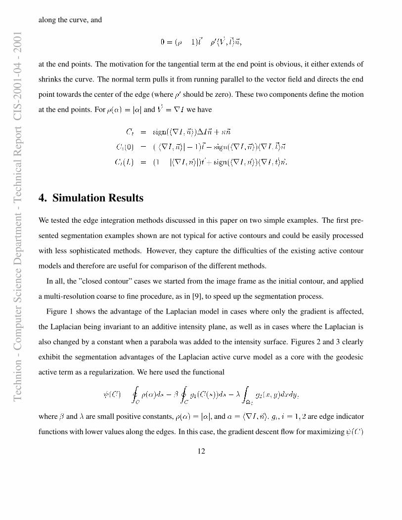
along the curve, and

9 � � 0 < ; �Ku < 0�¥ �

K� � Ku � KL �at the end points. The motivation for the tangential term at the end point is obvious, it either extends of

shrinks the curve. The normal term pulls it from running parallel to the vector field and directs the end

point towards the center of the edge (where 0 ¥ should be zero). These two components define the motion

at the end points. For 0 � Z*� ��N Z N and

K� � � � we have$ ¯ � V£�� "¡ �+� � � � KLf� �ñs � KL �.� KL$ ¯ � 9 � � � N � � � � KLf� N < ; �Ku < V£�� ¸¡ � �� KLf� �� Ku � KL$ ¯ � Y � � � ; < N � � � � KLf� N � Ku � V£�� "¡ �+� � � � KL� �� Ku � KL t

4. Simulation Results

We tested the edge integration methods discussed in this paper on two simple examples. The first pre-

sented segmentation examples shown are not typical for active contours and could be easily processed

with less sophisticated methods. However, they capture the difficulties of the existing active contour

models and therefore are useful for comparison of the different methods.

In all, the ”closed contour” cases we started from the image frame as the initial contour, and applied

a multi-resolution coarse to fine procedure, as in [9], to speed up the segmentation process.

Figure 1 shows the advantage of the Laplacian model in cases where only the gradient is affected,

the Laplacian being invariant to an additive intensity plane, as well as in cases where the Laplacian is

also changed by a constant when a parabola was added to the intensity surface. Figures 2 and 3 clearly

exhibit the segmentation advantages of the Laplacian active curve model as a core with the geodesic

active term as a regularization. We here used the functional( � $ � �¹[�] 0 ��ZX� A % <kò [³] ¿ � � $ � %"� � A % <ôó ,�h i ¿ � �� A � A ��where ò and ó are small positive constants, 0 ��ZX� �ON Z N , and

Z � � � � � KLf� . ¿Jõ , ö*� ; ��÷ are edge indicator

functions with lower values along the edges. In this case, the gradient descent flow for maximizing( � $ �

12

Tec

hnio

n - C

ompu

ter S

cien

ce D

epar

tmen

t - T

echn

ical

Rep

ort

CIS

-200

1-04

- 20

01

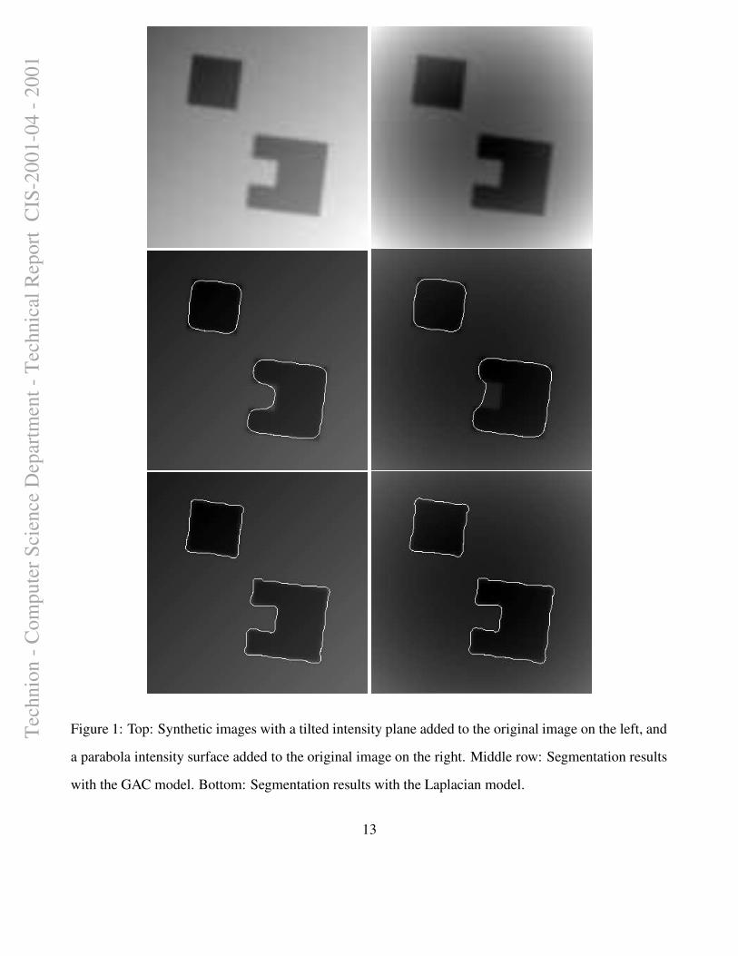
Figure 1: Top: Synthetic images with a tilted intensity plane added to the original image on the left, and

a parabola intensity surface added to the original image on the right. Middle row: Segmentation results

with the GAC model. Bottom: Segmentation results with the Laplacian model.

13

Tec

hnio

n - C

ompu

ter S

cien

ce D

epar

tmen

t - T

echn

ical

Rep

ort

CIS

-200

1-04

- 20

01

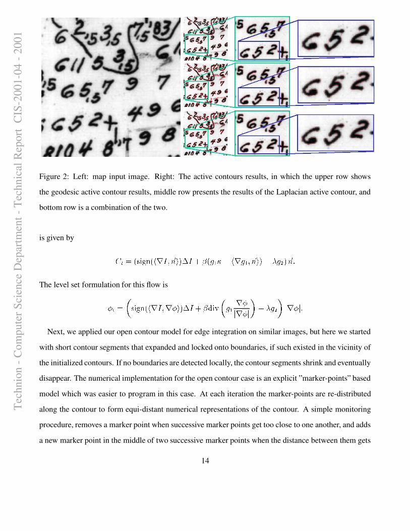
Figure 2: Left: map input image. Right: The active contours results, in which the upper row shows

the geodesic active contour results, middle row presents the results of the Laplacian active contour, and

bottom row is a combination of the two.

is given by $ ¯ � � V£�� ¸¡ � �� KL�� s � � ò � ¿ � � < �� ¿ � �KL�� <½ó ¿ � �

KL tThe level set formulation for this flow is°E¯ø��dEV£�� "¡ � �� ° � ��s � � ò ��ùd ¿ � � °N � °¬N g <½ó ¿ � g N � °¬N t

Next, we applied our open contour model for edge integration on similar images, but here we started

with short contour segments that expanded and locked onto boundaries, if such existed in the vicinity of

the initialized contours. If no boundaries are detected locally, the contour segments shrink and eventually

disappear. The numerical implementation for the open contour case is an explicit ”marker-points” based

model which was easier to program in this case. At each iteration the marker-points are re-distributed

along the contour to form equi-distant numerical representations of the contour. A simple monitoring

procedure, removes a marker point when successive marker points get too close to one another, and adds

a new marker point in the middle of two successive marker points when the distance between them gets

14

Tec

hnio

n - C

ompu

ter S

cien

ce D

epar

tmen

t - T

echn

ical

Rep

ort

CIS

-200

1-04

- 20

01

larger than a given threshold. The examples show how initial segments expand and deform until they

lock onto the boundaries of rather complex shapes. See Figures 4 and 5.

5. Conclusions

In this paper we proposed to incorporate the directional information that is generally ignored when de-

signing edge integration methods in a variational framework. Simulations that were performed with

the newly defined edge integration processes amply demonstrated their excellent performance as com-

pared to the best existing edge integration methods. Our extended active contour models are just a few

examples of the many possible combinations of geometric measures. Other functionals that could be

considered to either open or closed curves are Y ) < Y ¾ , or è 0 ��ZX�ñú�� N � �PN � A % , for an edge indicator func-

tion likeú � ; < ¿ � N � �fN � or

ú^� N � �fN � �üû N � �PN � � ; . For closed curves, the(e)

part is most effective

when the curve is close to its final location, therefore, the functional ý{� 0 � Z*�� ; < ¿ � < ¿ � A % could also be

considered.

Acknowledgments

We thank Evgeni Krimer and Roman Barsky for implementing and testing the open active contours

models.

References

[1] V. Caselles, F. Catte, T. Coll, and F. Dibos. A geometric model for active contours. Numerische

Mathematik, 66:1–31, 1993.

[2] V. Caselles, R. Kimmel, and G. Sapiro. Geodesic active contours. IJCV, 22(1):61–79, 1997.

[3] P. Fua and Y. G. Leclerc. Model driven edge detection. Machine Vision and Applications, 3:45–56,

1990.

15

Tec

hnio

n - C

ompu

ter S

cien

ce D

epar

tmen

t - T

echn

ical

Rep

ort

CIS

-200

1-04

- 20

01

[4] M. Kass, A. Witkin, and D. Terzopoulos. Snakes: Active contour models. International Journal of

Computer Vision, 1:321–331, 1988.

[5] R. Malladi, J. Sethian, and B. C. Vemuri. Shape modeling with front propagation: A level set

approach. IEEE Trans. on PAMI, 17:158–175, 1995.

[6] D. Marr. Vision. Freeman, San Francisco, 1982.

[7] D. Marr and E. Hildreth. Theory of edge detection. Proc. of the Royal Society London B, 207:187–

217, 1980.

[8] S. J. Osher and J. Sethian. Fronts propagating with curvature dependent speed: Algorithms based

on Hamilton-Jacobi formulations. J. of Comp. Phys., 79:12–49, 1988.

[9] N. Paragios and R. Deriche. Geodesic active contours and level sets for the detection and tracking

of moving objects. IEEE Trans. on PAMI, 22(3):266–280, 2000.

[10] N. K. Paragios, O. Mellina-Gotardo, and V. Ramesh. Gradient vector flow fast geodesic active

contours. In Proceedings ICCV’95, Vancouver, Canada, July 2001.

[11] J. Sethian. Level Set Methods: Evolving Interfaces in Geometry, Fluid Mechanics, Computer Vision

and Materials Sciences. Cambridge Univ. Press, 1996.

[12] A. Vasilevskiy and K. Siddiqi. Flux maximizing geometric flows. In Proceedings ICCV’95, Van-

couver, Canada, July 2001.

[13] C. Xu and J. Prince. Snakes, shapes, and gradient vector flow. IEEE Trans. IP, 7(3):359–369,

1998.

16

Tec

hnio

n - C

ompu

ter S

cien

ce D

epar

tmen

t - T

echn

ical

Rep

ort

CIS

-200

1-04

- 20

01

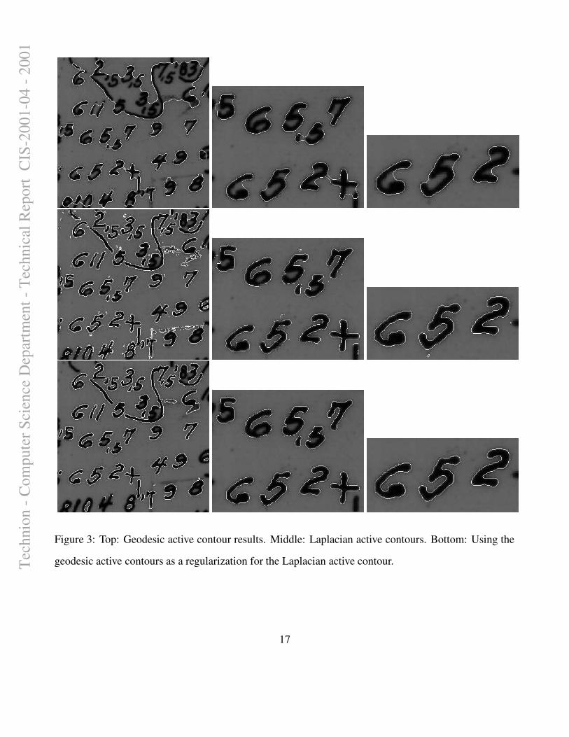
Figure 3: Top: Geodesic active contour results. Middle: Laplacian active contours. Bottom: Using the

geodesic active contours as a regularization for the Laplacian active contour.

17

Tec

hnio

n - C

ompu

ter S

cien

ce D

epar

tmen

t - T

echn

ical

Rep

ort

CIS

-200

1-04

- 20

01

time=0 time=50 time=100 time=150



Figure 4: Open geometric Laplacian active contours: The initial small diagonal lines (top left frame)

deform and either shrink and vanish or extend along the boundaries of the objects and capture their

shapes.

18

Tec

hnio

n - C

ompu

ter S

cien

ce D

epar

tmen

t - T

echn

ical

Rep

ort

CIS

-200

1-04

- 20

01




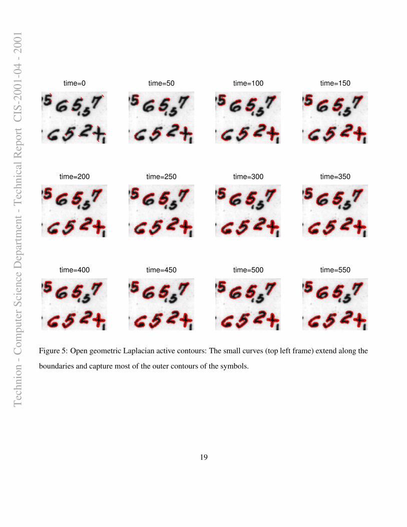
Figure 5: Open geometric Laplacian active contours: The small curves (top left frame) extend along the

boundaries and capture most of the outer contours of the symbols.

19

Tec

hnio

n - C

ompu

ter S

cien

ce D

epar

tmen

t - T

echn

ical

Rep

ort

CIS

-200

1-04

- 20

01

regularized laplacian zero crossings as optimal edge...

Documents