regularizing deep networks with semantic data augmentation

IEEE TRANSACTIONS ON PATTERN ANALYSIS AND MACHINE INTELLIGENCE 1

Regularizing Deep Networks with SemanticData Augmentation

Yulin Wang∗, Gao Huang∗, Member, IEEE , Shiji Song, Senior Member, IEEE , Xuran Pan, Yitong Xia,and Cheng Wu

Abstract—Data augmentation is widely known as a simple yet surprisingly effective technique for regularizing deep networks.Conventional data augmentation schemes, e.g., flipping, translation or rotation, are low-level, data-independent and class-agnosticoperations, leading to limited diversity for augmented samples. To this end, we propose a novel semantic data augmentation algorithm tocomplement traditional approaches. The proposed method is inspired by the intriguing property that deep networks are effective inlearning linearized features, i.e., certain directions in the deep feature space correspond to meaningful semantic transformations, e.g.,changing the background or view angle of an object. Based on this observation, translating training samples along many such directionsin the feature space can effectively augment the dataset for more diversity. To implement this idea, we first introduce a sampling basedmethod to obtain semantically meaningful directions efficiently. Then, an upper bound of the expected cross-entropy (CE) loss on theaugmented training set is derived by assuming the number of augmented samples goes to infinity, yielding a highly efficient algorithm. Infact, we show that the proposed implicit semantic data augmentation (ISDA) algorithm amounts to minimizing a novel robust CE loss,which adds minimal extra computational cost to a normal training procedure. In addition to supervised learning, ISDA can be applied tosemi-supervised learning tasks under the consistency regularization framework, where ISDA amounts to minimizing the upper bound ofthe expected KL-divergence between the augmented features and the original features. Although being simple, ISDA consistentlyimproves the generalization performance of popular deep models (e.g., ResNets and DenseNets) on a variety of datasets, i.e., CIFAR-10,CIFAR-100, SVHN, ImageNet, and Cityscapes. Code for reproducing our results is available athttps://github.com/blackfeather-wang/ISDA-for-Deep-Networks.

Index Terms—Data augmentation, deep learning, semi-supervised learning.

F

1 INTRODUCTION

DATA augmentation is an effective technique to alleviatethe overfitting problem in training deep networks

[1], [2], [3], [4], [5]. In the context of image recognition,this usually corresponds to applying content preservingtransformations, e.g., cropping, horizontal mirroring, rotationand color jittering, on the input samples. Although beingeffective, these augmentation techniques are not capableof performing semantic transformations, such as changingthe background of an object or the texture of a foregroundobject. Recent work has shown that data augmentation can bemore powerful if these (class identity preserving) semantictransformations are allowed [6], [7], [8]. For example, bytraining a generative adversarial network (GAN) for eachclass in the training set, one could then sample an infinitenumber of samples from the generator. Unfortunately, thisprocedure is computationally intensive because traininggenerative models and inferring them to obtain augmentedsamples are both nontrivial tasks. Moreover, due to the extraaugmented data, the training procedure is also likely to beprolonged.

• Y. Wang, G. Huang, S. Song, X. Pan and C. Wu are with the Departmentof Automation, BNRist, Tsinghua University, Beijing 100084, China.Email: {wang-yl19, pxr18}@mails.tsinghua.edu.cn, {gaohuang, shijis,wuc}@tsinghua.edu.cn. Corresponding author: Gao Huang.

• Y. Xia is with the School of Automation Science and Electrical Engineering,Beihang University, Beijing, China. Email: [email protected]∗. Equal contribution.

Traditional Data Augmentation

Semantic Data Augmentation

Flipping Rotating Translating

Changing Color Changing Background

Changing Visual Angle

…

…

Fig. 1. The comparison of traditional and semantic data augmentation.Conventionally, data augmentation usually corresponds to naive imagetransformations (like flipping, rotating, translating, etc.) in the pixelspace. Performing class identity preserving semantic transformations(like changing the color of a car, changing the background of an object,etc.) is another effective approach to augment the training data, which iscomplementary to traditional techniques.

In this paper, we propose an implicit semantic dataaugmentation (ISDA) algorithm for training deep networks.The ISDA is highly efficient as it does not require train-ing/inferring auxiliary networks or explicitly generatingextra training samples. Our approach is motivated by theintriguing observation made by recent work showing thatthe features deep in a network are usually linearized [9],[10]. Specifically, there exist many semantic directions in thedeep feature space, such that translating a data sample inthe feature space along one of these directions results in afeature representation corresponding to another sample withthe same class identity but different semantics. For example,

c©2021 IEEE. Personal use of this material is permitted. Permission from IEEE must be obtained for all other uses, in any current or future media, includingreprinting/republishing this material for advertising or promotional purposes, creating new collective works, for resale or redistribution to servers or lists, or reuse ofany copyrighted component of this work in other works.


Deep Features Augmented SamplesDeep Feature Space Forward

Augment Semantically

Augmented Images(Not Shown Explicitly)

Training Data

Corresponding to

ISDA Loss

… Deep Networks

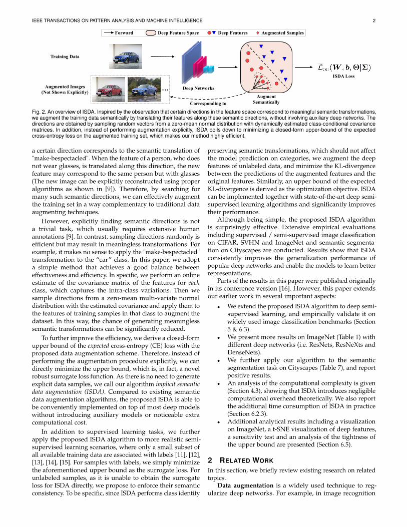
Fig. 2. An overview of ISDA. Inspired by the observation that certain directions in the feature space correspond to meaningful semantic transformations,we augment the training data semantically by translating their features along these semantic directions, without involving auxiliary deep networks. Thedirections are obtained by sampling random vectors from a zero-mean normal distribution with dynamically estimated class-conditional covariancematrices. In addition, instead of performing augmentation explicitly, ISDA boils down to minimizing a closed-form upper-bound of the expectedcross-entropy loss on the augmented training set, which makes our method highly efficient.

a certain direction corresponds to the semantic translation of"make-bespectacled". When the feature of a person, who doesnot wear glasses, is translated along this direction, the newfeature may correspond to the same person but with glasses(The new image can be explicitly reconstructed using properalgorithms as shown in [9]). Therefore, by searching formany such semantic directions, we can effectively augmentthe training set in a way complementary to traditional dataaugmenting techniques.

However, explicitly finding semantic directions is nota trivial task, which usually requires extensive humanannotations [9]. In contrast, sampling directions randomly isefficient but may result in meaningless transformations. Forexample, it makes no sense to apply the "make-bespectacled"transformation to the “car” class. In this paper, we adopta simple method that achieves a good balance betweeneffectiveness and efficiency. In specific, we perform an onlineestimate of the covariance matrix of the features for eachclass, which captures the intra-class variations. Then wesample directions from a zero-mean multi-variate normaldistribution with the estimated covariance and apply them tothe features of training samples in that class to augment thedataset. In this way, the chance of generating meaninglesssemantic transformations can be significantly reduced.

To further improve the efficiency, we derive a closed-formupper bound of the expected cross-entropy (CE) loss with theproposed data augmentation scheme. Therefore, instead ofperforming the augmentation procedure explicitly, we candirectly minimize the upper bound, which is, in fact, a novelrobust surrogate loss function. As there is no need to generateexplicit data samples, we call our algorithm implicit semanticdata augmentation (ISDA). Compared to existing semanticdata augmentation algorithms, the proposed ISDA is able tobe conveniently implemented on top of most deep modelswithout introducing auxiliary models or noticeable extracomputational cost.

In addition to supervised learning tasks, we furtherapply the proposed ISDA algorithm to more realistic semi-supervised learning scenarios, where only a small subset ofall available training data are associated with labels [11], [12],[13], [14], [15]. For samples with labels, we simply minimizethe aforementioned upper bound as the surrogate loss. Forunlabeled samples, as it is unable to obtain the surrogateloss for ISDA directly, we propose to enforce their semanticconsistency. To be specific, since ISDA performs class identity

preserving semantic transformations, which should not affectthe model prediction on categories, we augment the deepfeatures of unlabeled data, and minimize the KL-divergencebetween the predictions of the augmented features and theoriginal features. Similarly, an upper bound of the expectedKL-divergence is derived as the optimization objective. ISDAcan be implemented together with state-of-the-art deep semi-supervised learning algorithms and significantly improvestheir performance.

Although being simple, the proposed ISDA algorithmis surprisingly effective. Extensive empirical evaluationsincluding supervised / semi-supervised image classificationon CIFAR, SVHN and ImageNet and semantic segmenta-tion on Cityscapes are conducted. Results show that ISDAconsistently improves the generalization performance ofpopular deep networks and enable the models to learn betterrepresentations.

Parts of the results in this paper were published originallyin its conference version [16]. However, this paper extendsour earlier work in several important aspects:

• We extend the proposed ISDA algorithm to deep semi-supervised learning, and empirically validate it onwidely used image classification benchmarks (Section5 & 6.3).

• We present more results on ImageNet (Table 1) withdifferent deep networks (i.e. ResNets, ResNeXts andDenseNets).

• We further apply our algorithm to the semanticsegmentation task on Cityscapes (Table 7), and reportpositive results.

• An analysis of the computational complexity is given(Section 4.3), showing that ISDA introduces negligiblecomputational overhead theoretically. We also reportthe additional time consumption of ISDA in practice(Section 6.2.3).

• Additional analytical results including a visualizationon ImageNet, a t-SNE visualization of deep features,a sensitivity test and an analysis of the tightness ofthe upper bound are presented (Section 6.5).

2 RELATED WORK

In this section, we briefly review existing research on relatedtopics.

Data augmentation is a widely used technique to reg-ularize deep networks. For example, in image recognition


tasks, augmentation methods like random flipping, mirroringand rotation are applied to enforce the geometric invarianceof convolutional networks [3], [4], [5], [17]. These classictechniques are fundamental to obtain highly generalizeddeep models. It is shown in some literature that abandoningcertain information in training images is also an effectiveapproach to augment the training data. Cutout [18] andrandom erasing [19] randomly cut a rectangle region ofan input image out to perform augmentation. In addi-tion, several studies focus on automatic data augmentationtechniques. E.g., AutoAugment [20] is proposed to searchfor a better augmentation strategy among a large pool ofcandidates using reinforcement learning. A key concern onAutoAugment is that the searching algorithm suffers from ex-tensive computational and time costs. Similar to our method,learning with marginalized corrupted features [21] can beviewed as an implicit data augmentation technique, but itis limited to simple linear models. Feature transfer learning[22] explicitly augments the under-represented data in thefeature space, while it merely focuses on the imbalance faceimages. Complementarily, recent research shows that seman-tic data augmentation techniques which apply class identitypreserving transformations (e.g. changing backgrounds ofobjects or varying visual angles) to the training data areeffective as well [6], [8], [23], [24]. This is usually achieved bygenerating extra semantically transformed training sampleswith specialized deep structures such as DAGAN [8], domainadaptation networks [24], or other GAN-based generators[6], [23]. Although being effective, these approaches arenontrivial to implement and computationally expensive, dueto the need to train generative models beforehand and inferthem during training.

Robust loss function. As shown in the paper, ISDAamounts to minimizing a novel robust loss function. There-fore, we give a brief review of related work on this topic.Recently, several robust loss functions are proposed toimprove the generalization performance of deep networks.For example, the Lq loss [25] is a balanced form betweenthe cross entropy (CE) loss and mean absolute error (MAE)loss, derived from the negative Box-Cox transformation. It isdesigned to achieve the robustness against corrupted labelsin the training set, but also achieves effective performanceto improve the generalization performance. Focal loss [26]attaches high weights to a sparse set of hard examples toprevent the vast number of easy samples from dominatingthe training of the network. The idea of introducing alarge decision margin for CE loss has been studied in [27],[28], [29]. These researches propose to maximize the cosinedistance between deep features of samples from differentclasses, in order to alleviate the overfitting brought by thedistribution gap between the training data and the realdistribution. In [30], the CE loss and the contrastive lossare combined to learn more discriminative features. Froma similar perspective, center loss [31] simultaneously learnsa center for deep features of each class and penalizes thedistances between the samples and their correspondingclass centers in the feature space, enhancing the intra-classcompactness and inter-class separability.

Semantic transformations via deep features. Our workis inspired by the fact that high-level representations learnedby deep convolutional networks can potentially capture

abstractions with semantics [10], [32]. In fact, translatingdeep features along certain directions has been shownto be corresponding to performing meaningful semantictransformations on the input images. For example, deepfeature interpolation [9] leverages linear interpolations ofdeep features from a pre-trained neural network to edit thesemantics of images. Variational Autoencoder (VAE) andGenerative Adversarial Network (GAN) based methods [33],[34], [35] establish a latent representation corresponding tothe abstractions of images, which can be manipulated toperform semantic transformations. Generally, these methodsreveal that there exist some semantically meaningful direc-tions in the deep feature space, which can be leveraged toperform semantic data augmentation efficiently.

Uncertainty modeling. Similar to us, some of previousworks on deep learning with uncertainty [36], [37], [38]also assume a Gaussian distribution for the deep featureor prediction of each sample. For example, in the context offace recognition and person re-identification, the probabilisticrepresentations are leveraged to address the issues of ambigu-ous faces [39] and data outliers/label noises [40]. In multi-task learning, the homoscedastic task uncertainty is used tolearn the weights of different tasks [41]. This technique isalso exploited to object detection to model the uncertaintyof bounding boxes [42]. Given that the proposed ISDAalgorithm aims at augmenting training data semantically, ourmotivation is fundamentally different from these works. Inaddition, ISDA involves novel techniques such as estimatingclass-conditional covariance matrices and the derivation ofthe surrogate loss.

Deep semi-supervised learning. Since ISDA can also beapplied to semi-supervised learning tasks, we also brieflyreview recent work in this field. For modern deep learning,the precise annotations of a sufficiently large training set areusually expensive and time-consuming to acquire. To savethe cost of annotation, a nice solution is training models ona small set of labeled data together with a large number ofunlabeled samples, which is named semi-supervised learning.The main methods on this topic can be divided into two sorts,teacher-based methods and perturbation-based methods. Theformer establish a ‘teacher model’ to provide supervisionfor unlabeled data. For example, temporal ensemble [15]uses the moving averaged prediction of the model onunannotated samples as pseudo labels. Mean teacher [14]performs an exponential moving average on the parametersof models to obtain a teacher network. On the other hand,perturbation-based methods add small perturbations to theinput images and enforce the prediction consistency of thenetwork between the perturbed images and original images.VAT [13] proposes to apply adversarial perturbations. Π-model [15] minimizes the mean-square distance betweenthe same image with different augmentation schemes. Asan augmentation technique, the proposed semi-supervisedISDA algorithm is complementary to both the two types ofmethods.

3 SEMANTIC TRANSFORMATIONS IN DEEP FEA-TURE SPACE

Deep networks have been known to excel at extracting high-level representations in the deep feature space [4], [5], [9],


Deep Networks


Changing Background

Changing Color

Deep Feature Space

Deep Features

Semantic Directions

Corresponding to

Fig. 3. An illustration of the insight from deep feature interpolation[9] and other existing works [10], [44], which inspires our method.Transformations like ‘changing the color of the car’ or ‘changing thebackground of the image’ can be realized by linearly translating thedeep features towards the semantic directions corresponding to thesetransformations.

[43], where the semantic relationships between samples canbe captured by the spatial positions of their deep features[10]. It has been shown in previous work that translatingdeep features towards certain directions corresponds tomeaningful semantic transformations when the features aremapped back to the input space [9], [10], [44]. As a matterof fact, such an observation can be leveraged to edit thesemantics of images without the help of deep architectures.An example is shown in Figure 3. Consider feeding animage of a blue car into the deep network and obtainingits deep feature. Then if we translate the deep feature alongthe directions corresponding to ‘change-color’ or ‘change-background’, we will get the deep features corresponding tothe images of the same car but with a red paint or under adifferent background.

Based on this intriguing property, we propose to directlyaugment the semantics of training data by translating theircorresponding deep features along many meaningful seman-tic directions. Our method is highly efficient compared withtraditional approaches of performing semantic augmentation.Conventionally, to achieve semantic changes, one needs totrain, deploy and infer deep generators such as cycle-GAN[34] or W-GAN [45]. The procedure is both computationallyexpensive and time-consuming. In contrast, translating deepfeatures just introduces the negligible computational cost oflinear interpolation.

One may challenge that although semantic transforma-tions are efficient to be realized via deep features, showingthe results out in the pixel space is difficult [9]. However,our goal is not to edit the semantic contents and obtain theresults, but to train deep networks with these semanticallyaltered images for the data augmentation purpose. Since theaugmented features can be directly used for training, it is notnecessary to explicitly show the semantic transformationswe perform. In the following, we will show that our methodintegrates the augmentation procedure into the trainingprocess of deep networks.

4 IMPLICIT SEMANTIC DATA AUGMENTATION(ISDA)As aforementioned, certain directions in the deep featurespace correspond to meaningful semantic transformations

like ‘make-bespectacled’ or ‘change-visual-angle’. By lever-aging this observation, we propose an implicit semantic dataaugmentation (ISDA) approach to augment the training setsemantically via deep features. Our method has two impor-tant components, i.e., online estimation of class-conditionalcovariance matrices and optimization with a robust lossfunction. The first component aims to find a distribution fromwhich we can sample meaningful semantic transformationdirections for data augmentation, while the second saves usfrom explicitly generating a large amount of extra trainingdata, leading to remarkable efficiency compared to existingdata augmentation techniques.

4.1 Semantic Direction Sampling

A challenge faced by our method is how to obtain suitablesemantic directions for augmentation. The directions needto correspond to the semantic transformations that aremeaningful for the main object in the image, while donot change the class identity of the image. For example,transformations like wearing glasses or dressing up aresuitable to augment the images of persons, but others likeflying or sailing are meaningless. In addition, it is obviousthat persons in the images should not be transformed tohorses or other objects that do not belong to their originalclass.

Previous work [9] proposes to find semantic directionsby human annotation. Their method is shown in Figure 4(a). Take changing the color of a car from blue to red forexample. Firstly, they collect two sets of images of blue carsand red cars, respectively, and fed them into deep networksto obtain their deep features. Then they take the vector fromthe average feature of blue cars to the average feature ofred cars. The vector corresponds to the transformation of‘changing the color of the car from blue to red’. At last, for anew image to transform, they translate its deep feature alongthe vector, and map the feature back to the pixel space. It hasbeen shown that their method is able to perform the specifictransformation precisely [9]. Whereas, human annotationis not a feasible approach in the context of semantic dataaugmentation. For one thing, one needs to collect sufficientannotated images for each possible transformation of eachclass. This procedure is inefficient. For another, it is difficultto pre-define all possible semantic transformations for eachclass. The omission will lead to inferior performance.

In terms of efficiency, a possible solution is to obtainsemantic directions by random sampling. However, sincethe deep feature space is highly sparse (e.g., ResNets [4]generate 64-dimensional features on CIFAR. Even if eachdimension has two possible values, there will be 264 possiblefeatures.), sampling totally at random will yield manymeaningless semantic directions. As shown in Figure 4(b), transformations like ‘getting older’ or ‘flying’ may beperformed for a car.

To achieve a nice trade-off between the effectivenessand efficiency, we propose to approximate the procedureof human annotation by sampling random vectors froma zero-mean normal distribution with a covariance that isproportional to the intra-class covariance matrix of samples tobe augmented. The covariance matrix captures the varianceof samples in that class and is thus likely to contain rich


Changing Color

(a) Human Annotation

Wearing Glassess Flying

Dressing up

SailingGetting Older

Barking

SpreadingWings

(b) Random Sampling

EstimatingCovariance

Matrices

Augment Samples in the Corresponding Class

Changing Background


Changing Color

…Getting Older

Wearing Glassess

Dressing up

(c) Class-Conditional Gaussian Sampling

Meaningless Semantic DirectionsDeep Feature Space Deep Features

MeaningfulSemantic Directions

Corresponding to

Changing Color

Cars Persons

…

Deep Features of Classes

Cars Persons

Fig. 4. Three different ways to obtain semantic directions for augmentation in the deep feature space. Human annotation is the most precise way. Butit requires collecting annotated images for each transformation of each class in advance, which is expensive and time-consuming. In addition, it willinevitably omit potential augmentation transformations. In contrast, finding semantic directions by random sampling is highly efficient, but yields alarge number of meaningless transformations. To achieve a nice trade-off between effectiveness and efficiency, we propose to estimate a covariancematrix for the deep features of each class, and sample semantic directions from a zero-mean normal distribution with the estimated class-conditionalcovariance matrix. The covariance matrix captures the intra-class feature distribution of the training data, and therefore contains rich information ofpotential semantic transformations.

semantic information. Intuitively, features of the person classmay vary along the ‘wearing glasses’ direction, as bothimages of persons with glasses and persons without glassesare contained in the training set. In contrast, the variancealong the ‘having propeller’ direction will be nearly zero asall persons do not have propellers. Similarly, features of theplane class may vary along the ‘having propeller’ direction,but will have nearly zero variance along the ‘wearing glasses’direction. We hope that directions corresponding to mean-ingful transformations for each class are well represented bythe principal components of the covariance matrix of thatclass. In addition to its efficiency, the proposed approach canactually leverage more potential semantic transformationsthan human annotation, as the obtained semantic directionsare continuously distributed in the deep feature space.

Consider training a deep network G with weights Θon a training set D = {(xi, yi)}, where yi ∈ {1, . . . , C}is the label of the ith sample xi over C classes. Let the A-dimensional vector ai = [ai1, . . . , aiA]T = G(xi,Θ) denotethe deep feature of xi learned by G, and aij indicate the jth

element of ai.

To obtain semantic directions to augment ai, we establisha zero-mean multi-variate normal distribution N (0,Σyi),where Σyi is the class-conditional covariance matrix esti-mated from the features of all the samples in class yi. Inimplementation, the covariance matrix is computed in an

online fashion by aggregating statistics from all mini-batches.Formally, the online estimation algorithm for the covariancematrices is given by:

µ(t)j =

n(t−1)j µ

(t−1)j +m

(t)j µ

′(t)j

n(t−1)j +m

(t)j

, (1)

Σ(t)j =

n(t−1)j Σ

(t−1)j +m

(t)j Σ′

(t)j

n(t−1)j +m

(t)j

+n

(t−1)j m

(t)j (µ

(t−1)j −µ′(t)j )(µ

(t−1)j −µ′(t)j )T

(n(t−1)j +m

(t)j )2

,

(2)

n(t)j = n

(t−1)j +m

(t)j , (3)

where µ(t)j and Σ

(t)j are the estimates of average values and

covariance matrices of the features of jth class at tth step. µ′(t)jand Σ′

(t)j are the average values and covariance matrices of

the features of jth class in tth mini-batch. n(t)j denotes the

total number of training samples belonging to jth class inall t mini-batches, and m(t)

j denotes the number of trainingsamples belonging to jth class only in tth mini-batch.

During training, C covariance matrices are computed,one for each class. The augmented feature ai is obtained


by translating ai along a random direction sampled fromN (0, λΣyi). Equivalently, we have:

ai ∼ N (ai, λΣyi), (4)

where λ is a positive coefficient to control the strengthof semantic data augmentation. As the covariances arecomputed dynamically during training, the estimation in thefirst few epochs is not quite informative when the network isnot well trained. To address this issue, we let λ = (t/T )×λ0

be a function of the current iteration t, thus to reduce theimpact of the estimated covariances on our algorithm earlyin the training stage.

4.2 Upper Bound of the Expected LossA naive method to implement the semantic data augmenta-tion is to explicitly augment each ai for M times, formingan augmented feature set {(a1

i , yi), . . . , (aMi , yi)}Ni=1 of size

MN , where ami is mth sample of augmented features forsample xi. Then the networks are trained by minimizing thecross-entropy (CE) loss:

LM (W , b,Θ)=1

N

N∑i=1

1

M

M∑m=1

− log(ew

Tyi

ami +byi∑Cj=1 e

wTjami +bj

), (5)

where W = [w1, . . . ,wC ]T ∈ RC×A and b =[b1, . . . , bC ]T ∈ RC are the weight matrix and biases cor-responding to the final fully connected layer, respectively.

Obviously, the naive implementation is computationallyinefficient when M is large, as the feature set is enlargedby M times. In the following, we consider the case that Mgrows to infinity, and find that an easy-to-compute upperbound can be derived for the loss function, leading to ahighly efficient implementation.

In the case M → ∞, we are in fact considering theexpectation of the CE loss under all possible augmentedfeatures. Specifically, L∞ is given by:

L∞(W , b,Θ|Σ)=1

N

N∑i=1

Eai [− log(ew

Tyi

ai+byi∑Cj=1 e

wTj ai+bj

)]. (6)

If L∞ can be computed efficiently, then we can directlyminimize it without explicitly sampling augmented features.However, Eq. (6) is difficult to compute in its exact form.Alternatively, we find that it is possible to derive an easy-to-compute upper bound for L∞, as given by the followingproposition.

Proposition 1. Suppose that ai ∼ N (ai, λΣyi). Then we havean upper bound of L∞, given by:

L∞ ≤1

N

N∑i=1

− log(ew

Tyi

ai+byi∑Cj=1e

wTjai+bj+

λ2 vT

jyiΣyivjyi

) , L∞, (7)

where vjyi = wj −wyi .

Proof. According to the definition of L∞ in Eq. (6), we have:

L∞ =1

N

N∑i=1

Eai [log(C∑j=1

evTjyi

ai+(bj−byi ))] (8)

≤ 1

N

N∑i=1

log(C∑j=1

Eai [evTjyi

ai+(bj−byi )]) (9)

=1

N

N∑i=1

log(C∑j=1

evTjyi

ai+(bj−byi )+λ2 vT

jyiΣyivjyi ) (10)

=L∞. (11)

In the above, the Inequality (9) follows from the Jensen’sinequality E[logX] ≤ log E[X], as the logarithmic functionlog(·) is concave. The Eq. (10) is obtained by leveraging themoment-generating function:

E[etX ] = etµ+ 12σ

2t2 , X ∼ N (µ, σ2),

due to the fact that vTjyiai+(bj−byi) is a Gaussian random

variable, i.e.,

vTjyi ai+(bj−byi) ∼ N (vT

jyiai+(bj−byi), λvTjyiΣyivjyi).

Essentially, Proposition 1 provides a surrogate loss for ourimplicit data augmentation algorithm. Instead of minimizingthe exact loss function L∞, we can optimize its upper boundL∞ in a much more efficient way. Therefore, the proposedISDA boils down to a novel robust loss function, which canbe easily adopted by most deep models. In addition, wecan observe that when λ→ 0, which means no features areaugmented, L∞ reduces to the standard CE loss.

In summary, the proposed ISDA approach can be simplyplugged into deep networks as a robust loss function, andefficiently optimized with the stochastic gradient descent(SGD) algorithm. We present the pseudo code of ISDA inAlgorithm 1.

Algorithm 1 The ISDA algorithm.1: Input: D, λ0

2: Randomly initialize W , b and Θ3: for t = 0 to T do4: Sample a mini-batch {xi, yi}Bi=1 from D5: Compute ai = G(xi,Θ)6: Estimate the covariance matrices Σ1, Σ2, ..., ΣC7: Compute L∞ according to Eq. (7)8: Update W , b, Θ with SGD9: end for

10: Output: W , b and Θ

4.3 Complexity of ISDA

Here we present a theoretical analysis to show that ISDA doesnot involve notable additional computational cost. As shownabove, ISDA requires extra computation for estimating thecovariance matrices and computing the upper bound ofthe excepted loss. For a single sample, the computationalcomplexity of the former is O(D2) (using the online updateformulas Eqs. (1)(2)), while that of the later is O(C×D2),where D is the dimension of feature space. In comparison, atypical ConvNet with L layers requiresO(D2×K2×H×W×L)operations, where K is the filter kernel size, and H and Ware the height and width of feature maps. Consider ResNet-110 on CIFAR (C10 & C100) as an example, for which wehave K = 3, H =W = 8 and L= 109 (ignoring the last FC-layer), then the extra computation cost of ISDA is up to threeorders of magnitude less than the total computation cost of thenetwork. In our experiments, the results of both theoreticaland practical cost of ISDA are provided in Table 3.


5 ISDA FOR DEEP SEMI-SUPERVISED LEARNING

Deep networks have achieved remarkable success in super-vised learning tasks when fueled by sufficient annotatedtraining data. However, obtaining abundant annotations isusually costly and time-consuming in practice. In compari-son, collecting training samples without labels is a relativelyeasier task. The goal of deep semi-supervised learning is toimprove the performance of deep networks by leveragingboth labeled and unlabeled data simultaneously [11], [12],[14], [15]. In this section, we further introduce how to applythe proposed algorithm to semi-supervised learning tasks.

It is not straightforward to directly implement the afore-mentioned ISDA algorithm in semi-supervised learning,since unlabeled samples do not have ground truth labels,which are essential to compute the supervised ISDA lossL∞. Inspired by other consistency based semi-supervisedlearning methods [13], [14], [15], [46], we propose a semanticconsistency training approach to exploit unlabeled data inISDA. Our major insight here is that the prediction of agiven sample should not be significantly changed whenit is augmented, because ISDA performs class identitypreserving semantic transformations. In specific, we firstaugment the deep features of unlabeled data, and thenminimize the KL-divergence between the predictions of theaugmented samples and the corresponding original samples.Interestingly, we find it feasible to derive a closed-form upper-bound of the expected KL-divergence as a surrogate loss,which makes our semi-supervised ISDA algorithm highlyefficient, similar to the case of supervised learning. ISDA canbe incorporated into state-of-the-art deep semi-supervisedlearning algorithms to further improve their performance.

Consider training a deep network with weights Θ ona labeled training set DL = {(xL

i , yLi )} and an unlabeled

training set DU = {xUi }. For labeled samples, we simply

minimize the upper bound in Proposition 1. For unlabeledsamples, given an input xU

i , we first obtain its deep featureaUi and the corresponding prediction pU

i ∈ (0, 1)C . Then weobtain the augmented feature:

aUi ∼ N (aU

i , λΣyUi), yU

i = arg maxjpUij , (12)

where pUij indicates the jth element of pU

i and yUi is the pseudo

label of xUi . The covariance matrix ΣyU

iis estimated using

the deep features of labeled data.Then the prediction of aU

i is able to be calculated, denotedas pU

i . Since ISDA performs transformations that do not affectthe class identity of samples, we enforce pU

i and pUi to be

similar by minimizing the KL-divergence between them.As aU

i is a random variable, a straightforward approach toachieve that is to obtain M samples of aU

i and minimizethe averaged KL-divergence of all the M samples. However,as discussed in Section 4.2, such a naive implementation isinefficient due to the enlarged feature set. To alleviate theproblem, we consider the case where M →∞ and minimizethe expected KL-divergence over aU

i :

minW ,b,Θ

EaUi[DKL(pU

i ||pUi )]. (13)

Here, we treat pUi as a constant to stabilize the training

procedure following [13], [14], [15]. Formally, a semantic

consistency loss for unlabeled data is given by:

LU∞(W , b,Θ|Σ)=

1

N

N∑i=1

C∑k=1

pUikEai [− log(

ewTkai+bk∑C

j=1 ewTj ai+bj

)].(14)

It is difficult to compute Eq. (14) in the exact form. Therefore,instead of directly using Eq. (14) as the loss function, weshow in the following proposition that a closed-form upperbound of LU

∞ can be obtained as a surrogate loss. Similarto the supervised learning case, our semi-supervised ISDAalgorithm amounts to minimizing a novel robust loss, andcan be implemented efficiently.

Proposition 2. Suppose that aUi ∼ N (aU

i , λΣyUi). Then we have

an upper bound of LU∞, given by:

LU∞ ≤

1

N

N∑i=1

C∑k=1

−pUik log(

ewTkai+bk∑C

j=1ewTjai+bj+

λ2v

Tjk(ΣyU

i)vjk

) , LU∞,

(15)

where vjk = wj −wk.

Proof. According to Eq. (14), we have:

LU∞ =

C∑k=1

pUik

{1

N

N∑i=1

Eai [− log(ew

Tkai+bk∑C

j=1 ewTj ai+bj

)]

}(16)

≤C∑k=1

pUik

1

N

N∑i=1

− log(ew

Tkai+bk∑C

j=1ewTjai+bj+

λ2v

Tjk(ΣyU

i)vjk

)

(17)

=LU∞. (18)

In the above, Inequality (17) follows from the conclusion ofProposition 1.

In sum, the loss function of our method is given by:

LL∞ + η1L

U∞ + η2Lregularization, (19)

where LL∞ is the ISDA loss on labeled data. As most deep

semi-supervised learning algorithms model unlabeled datain regularization terms, they can be conveniently integratedwith ISDA by appending the corresponding regularizationterm Lregularization to the loss function. The coefficient η1

and η2 are pre-defined hyper-parameters to determine theimportance of different regularization terms.

6 EXPERIMENTS

In this section, we empirically validate the proposed algo-rithm on several tasks. First, we present the experimentalresults of supervised image classification on widely usedbenchmarks, i.e., CIFAR [1] and ImageNet [47]. Second,we show the performance of several deep semi-supervisedlearning algorithms with and without ISDA on CIFAR [1]and SVHN [48]. Third, we apply ISDA to the semanticsegmentation task on the Cityscapes dataset [49].

In addition, to demonstrate that ISDA encourages modelsto learn better representations, we conduct experiments byemploying the models trained with ISDA as backbones forthe object detection task and the instance segmentationtask on the MS COCO dataset [50], which are presentedin Appendix D.


Furthermore, a series of analytical experiments are con-ducted to provide additional insights into our algorithm.We provide the visualization results of both the augmentedsamples and the representations learned by deep networks.We also present the empirical results to check the tightnessof the upper bound used by ISDA. The performance of ex-plicit and implicit semantic data augmentation is compared.Finally, ablation studies and sensitivity tests are conductedto show how the components and hyper-parameters affectthe performance of ISDA.

6.1 Experimental Setups for Image Classification

Datasets. We use three image classification benchmarksin the experiments. (1) The two CIFAR datasets consistof 32x32 colored natural images in 10 classes for CIFAR-10 and 100 classes for CIFAR-100, with 50,000 images fortraining and 10,000 images for testing, respectively. (2) TheStreet View House Numbers (SVHN) dataset [48] consists of32x32 colored images of digits. 73,257 images for training,26,032 images for testing and 531,131 images for additionaltraining are provided. (3) ImageNet is a 1,000-class datasetfrom ILSVRC2012 [47], providing 1.2 million images fortraining and 50,000 images for validation.

Validation set and data pre-procession. (1) On CIFAR,in our supervised learning experiments, we hold out 5,000images from the training set as the validation set to searchfor the hyper-parameter λ0. These samples are also used fortraining after an optimal λ0 is selected, and the results onthe test set are reported. Images are normalized with channelmeans and standard deviations for pre-processing. We followthe basic data augmentation operations in [4], [5], [51], [52]:4 pixels are padded at each side of the image, followed by arandom 32x32 cropping combined with random horizontalflipping. In semi-supervised learning experiments, we holdout 25% of labeled images as the validation set to select λ0, η1

and η2, following [13]. Similarly, these samples are also usedfor training with the selected hyper-parameters. Followingthe common practice of semi-supervised learning [13], [14],[15], [53], we apply ZCA whitening for pre-processing andrandom 2x2 translation followed by random horizontal flipfor basic augmentation. (2) The SVHN dataset is used forsemi-supervised learning experiments, where 25% of labeledimages are held out as the validation set. The validation setis put back for training after the hyper-parameter searching.Following [14], [46], we perform random 2x2 translation toaugment the training data. (3) On ImageNet, we adopt thesame augmentation configurations as [2], [4], [5], [54], [55].

Non-semantic augmentation techniques. To study thecomplementary effects of ISDA to traditional data augmen-tation methods, three state-of-the-art non-semantic augmen-tation techniques are applied with and without ISDA. (1)Cutout [18] randomly masks out square regions of inputsduring training. (2) AutoAugment [62] automatically searchesfor the best augmentation policy using reinforcement learn-ing. (3) RandAugment [61] searches for augmentation policiesusing grid search in a reduced searching space.

Baselines for supervised learning. Our method is com-pared with several baselines including state-of-the-art robustloss functions and generator-based semantic data augmenta-tion methods. (1) Dropout [68] is a widely used regularization

approach that randomly mutes some neurons during training.(2) Large-margin softmax loss [27] introduces a large decisionmargin, measured by a cosine distance, to the standard CEloss. (3) Disturb label [63] is a regularization mechanism thatrandomly replaces a fraction of labels with incorrect ones ineach iteration. (4) Focal loss [26] focuses on a sparse set ofhard examples to prevent easy samples from dominating thetraining procedure. (5) Center loss [31] simultaneously learns acenter of features for each class and minimizes the distancesbetween the deep features and their corresponding classcenters. (6) Lq loss [25] is a noise-robust loss function, usingthe negative Box-Cox transformation. (7) Label Smoothing [64]smooth the one-hot label to a soft one with equal valuesfor other classes. (8) DistributionNet [40] models the deepfeatures of training samples as Gaussian distributions, andlearns the covariance automatically. (9) For generator-basedsemantic augmentation methods, we train several state-of-the-art GANs [45], [65], [66], [67], which are then used togenerate extra training samples for data augmentation.

Baselines for semi-supervised learning. In semi-supervised learning experiments, the performance of ISDA istested on the basis of several modern deep semi-supervisedlearning approaches. (1) Π-model [15] enforces the model tohave the same prediction on a sample with different augmen-tation and dropout modes. (2) Temp-ensemble [15] attaches asoft pseudo label to each unlabeled sample by performinga moving average on the predictions of networks. (3) Meanteacher [14] establishes a teacher network by performing anexponential moving average on the parameters of the model,and leverages the teacher network to produce supervisionfor unlabeled data. (4) Virtual Adversarial Training (VAT) [13]adds adversarial perturbation to each sample and enforcesthe model to have the same prediction on the perturbedsamples and the original samples.

For a fair comparison, all methods are implemented withthe same training configurations. Details for hyper-parametersettings are presented in Appendix C.

Implementation details. For supervised learning, weimplement the ResNet, SE-ResNet, Wide-ResNet, ResNeXt,DenseNet and Shake-shake net on the two CIFAR datasets,and implement ResNet, DenseNet and ResNeXt on ImageNet.For semi-supervised learning, we implement the widely usedCNN-13 network [13], [14], [15], [46], [53], [69], [70]. Detailsfor implementing these models are given in Appendix A andAppendix B for supervised learning and semi-supervisedlearning, respectively. The hyper-parameter λ0 for ISDA isselected from the set {0.1, 0.25, 0.5, 0.75, 1} according to theperformance on the validation set. On ImageNet, due to GPUmemory limitation, we approximate the covariance matricesby their diagonals, i.e., the variance of each dimensionof the features. The best hyper-parameter λ0 is selectedfrom {1, 2.5, 5, 7.5, 10}. For semi-supervised learning tasks,the hyper-parameter η1 is selected from {0.5, 1, 2}. In allexperiments, the average test error of the last 10 epochs iscalculated as the result to be reported.

6.2 Supervised Image Classification

6.2.1 Main ResultsResults on ImageNet. Table 1 presents the performance ofISDA on the large scale ImageNet dataset with state-of-the-


TABLE 1Single crop error rates (%) of different deep networks on the validation set of ImageNet. We report the results of our implementation with and without

ISDA. The better results are bold-faced, while the numbers in brackets denote the performance improvements achieved by ISDA. For a faircomparison, we present the baselines reported by other papers [5], [56] as well. We also report the theoretical computational overhead and the

additional training time introduced by ISDA in the last two columns, which is obtained with 8 Tesla V100 GPUs.

Networks ParamsTop-1/Top-5 Error Rates (%) Additional Cost Additional Cost

Reported in [5], [56] Our Implementation ISDA (Theoretical) (Wall Time)ResNet-50 [4] 25.6M 23.7 / 7.1 23.0 / 6.8 21.9(1.1) / 6.3 0.25% 7.6%ResNet-101 [4] 44.6M 21.9 / 6.3 21.7 / 6.1 20.8(0.9) / 5.7 0.13% 7.4%ResNet-152 [4] 60.3M 21.7 / 5.9 21.3 / 5.8 20.3(1.0) / 5.5 0.09% 5.4%

DenseNet-BC-121 [5] 8.0M 25.0 / 7.7 23.7 / 6.8 23.2(0.5) / 6.6 0.20% 5.6%DenseNet-BC-265 [5] 33.3M 22.2 / 6.1 21.9 / 6.1 21.2(0.7) / 6.0 0.24% 5.4%

ResNeXt-50, 32x4d [57] 25.0M – / – 22.5 / 6.4 21.3(1.2) / 5.9 0.24% 6.6%ResNeXt-101, 32x8d [57] 88.8M – / – 21.1 / 5.9 20.1(1.0) / 5.4 0.06% 7.9%

TABLE 2Evaluation of ISDA on CIFAR with different models. We report mean values and standard deviations in five independent experiments. The better

results are bold-faced.

Networks ParamsCIFAR-10 CIFAR-100

Basic ISDA Basic ISDAResNet-32 [4] 0.5M 7.39 ± 0.10% 7.09 ± 0.12% 31.20 ± 0.41% 30.27 ± 0.34%

ResNet-110 [4] 1.7M 6.76 ± 0.34% 6.33 ± 0.19% 28.67 ± 0.44% 27.57 ± 0.46%SE-ResNet-110 [58] 1.7M 6.14 ± 0.17% 5.96 ± 0.21% 27.30 ± 0.03% 26.63 ± 0.21%

Wide-ResNet-16-8 [59] 11.0M 4.25 ± 0.18% 4.04 ± 0.29% 20.24 ± 0.27% 19.91 ± 0.21%Wide-ResNet-28-10 [59] 36.5M 3.82 ± 0.15% 3.58 ± 0.15% 18.53 ± 0.07% 17.98 ± 0.15%ResNeXt-29, 8x64d [57] 34.4M 3.86 ± 0.14% 3.67 ± 0.12% 18.16 ± 0.13% 17.43 ± 0.25%DenseNet-BC-100-12 [5] 0.8M 4.90 ± 0.08% 4.54 ± 0.07% 22.61 ± 0.10% 22.10 ± 0.34%

Shake-Shake (26, 2x32d) [60] 3.0M 3.45 ± 0.01% 3.20 ± 0.03% 20.12 ± 0.39% 19.45 ± 0.16%Shake-Shake (26, 2x112d) [60] 36.4M 2.92 ± 0.02% 2.61 ± 0.09% 17.42 ± 0.44% 16.73 ± 0.18%

TABLE 3The theoretical computational overhead and the empirical additional time consumption of ISDA on CIFAR. The results are obtained with a single

Tesla V100 GPU.

Networks

CIFAR-10 CIFAR-100Standard Additional Cost

Additional Cost(Wall Time)

Additional CostAdditional Cost

(Wall Time)FLOPs (Theoretical) (Theoretical)Absolute Relative Absolute Relative

ResNet-32 [4] 69.43M 0.05M 0.07% 1.85% 0.44M 0.63% 1.85%ResNet-110 [4] 254.20M 0.05M 0.02% 4.48% 0.44M 0.17% 2.94%

SE-ResNet-110 [58] 254.73M 0.05M 0.02% 2.17% 0.44M 0.17% 1.08%Wide-ResNet-16-8 [59] 1.55G 2.96M 0.19% 3.39% 27.19M 1.76% 10.77%Wide-ResNet-28-10 [59] 5.25G 4.61M 0.09% 2.37% 42.46M 0.81% 12.35%ResNeXt-29, 8x64d [57] 5.39G 11.80M 0.22% 1.90% 109.00M 2.02% 12.32%DenseNet-BC-100-12 [5] 292.38M 1.35M 0.46% 5.50% 12.43M 4.25% 12.03%

Shake-Shake (26, 2x32d) [60] 426.69M 0.19M 0.04% 5.77% 1.76M 0.41% 2.21%Shake-Shake (26, 2x112d) [60] 5.13G 2.31M 0.05% 3.85% 21.30M 0.42% 5.07%

art deep networks. It can be observed that ISDA significantlyimproves the generalization performance of these models.For example, the Top-1 error rate of ResNet-50 is reducedby 1.1% via being trained with ISDA, approaching the per-formance of ResNet-101 (21.9% v.s. 21.7%) with 43% fewerparameters. Similarly, the performance of ResNet-101+ISDAsurpasses that of ResNet-152 with 26% less parameters.Compared to ResNets, DenseNets generally suffer less fromoverfitting due to their architecture design, and thus appearto benefit less from our algorithm.

Results on CIFAR. We report the error rates of severalmodern deep networks with and without ISDA on CIFAR-10/100 in Table 2. Similar observations to ImageNet canbe obtained. On CIFAR-100, for relatively small models likeResNet-32 and ResNet-110, ISDA reduces test errors by about1%, while for larger models like Wide-ResNet-28-10 and

ResNeXt-29, 8x64d, our method outperforms the competitivebaselines by nearly 0.7%.

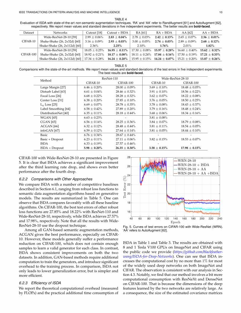
Complementing explicit augmentation techniques. Ta-ble 4 shows the experimental results with recently proposedtraditional image augmentation methods (i.e., Cutout [18],RandAugment [61] and AutoAugment [62]). Interestingly,ISDA seems to be even more effective when these techniquesexist. For example, when applying AutoAugment, ISDAachieves performance gains of 1.34% and 0.98% on CIFAR-100 with the Shake-Shake (26, 2x112d) and the Wide-ResNet-28-10, respectively. Note that these improvements are moresignificant than the standard situations. A plausible explana-tion for this phenomenon is that non-semantic augmentationmethods help to learn a better feature representation, whichmakes semantic transformations in the deep feature spacemore reliable. The curves of test errors during training on


TABLE 4Evaluation of ISDA with state-of-the-art non-semantic augmentation techniques. ‘RA’ and ‘AA’ refer to RandAugment [61] and AutoAugment [62],

respectively. We report mean values and standard deviations in five independent experiments. The better results are bold-faced.

Dataset Networks Cutout [18] Cutout + ISDA RA [61] RA + ISDA AA [62] AA + ISDA

CIFAR-10Wide-ResNet-28-10 [59] 2.99 ± 0.06% 2.83 ± 0.04% 2.78 ± 0.03% 2.42 ± 0.13% 2.65 ± 0.07% 2.56 ± 0.01%

Shake-Shake (26, 2x32d) [60] 3.16 ± 0.09% 2.93 ± 0.03% 3.00 ± 0.05% 2.74 ± 0.03% 2.89 ± 0.09% 2.68 ± 0.12%Shake-Shake (26, 2x112d) [60] 2.36% 2.25% 2.10% 1.76% 2.01% 1.82%

CIFAR-100Wide-ResNet-28-10 [59] 18.05 ± 0.25% 16.95 ± 0.11% 17.30 ± 0.08% 15.97 ± 0.28% 16.60 ± 0.40% 15.62 ± 0.32%

Shake-Shake (26, 2x32d) [60] 18.92 ± 0.21% 18.17 ± 0.08% 18.11 ± 0.24% 17.84 ± 0.16% 17.50 ± 0.19% 17.21 ± 0.33%Shake-Shake (26, 2x112d) [60] 17.34 ± 0.28% 16.24 ± 0.20% 15.95 ± 0.15% 14.24 ± 0.07% 15.21 ± 0.20% 13.87 ± 0.26%

TABLE 5Comparisons with the state-of-the-art methods. We report mean values and standard deviations of the test errors in five independent experiments.

The best results are bold-faced.

MethodResNet-110 Wide-ResNet-28-10

CIFAR-10 CIFAR-100 CIFAR-10 CIFAR-100Large Margin [27] 6.46 ± 0.20% 28.00 ± 0.09% 3.69 ± 0.10% 18.48 ± 0.05%Disturb Label [63] 6.61 ± 0.04% 28.46 ± 0.32% 3.91 ± 0.10% 18.56 ± 0.22%Focal Loss [26] 6.68 ± 0.22% 28.28 ± 0.32% 3.62 ± 0.07% 18.22 ± 0.08%Center Loss [31] 6.38 ± 0.20% 27.85 ± 0.10% 3.76 ± 0.05% 18.50 ± 0.25%Lq Loss [25] 6.69 ± 0.07% 28.78 ± 0.35% 3.78 ± 0.08% 18.43 ± 0.37%Label Smoothing [64] 6.58 ± 0.42% 27.89 ± 0.20% 3.79 ± 0.16% 18.48 ± 0.24%DistributionNet [40] 6.35 ± 0.11% 28.18 ± 0.44% 3.68 ± 0.06% 18.34 ± 0.16%WGAN [45] 6.63 ± 0.23% - 3.81 ± 0.08% -CGAN [65] 6.56 ± 0.14% 28.25 ± 0.36% 3.84 ± 0.07% 18.79 ± 0.08%ACGAN [66] 6.32 ± 0.12% 28.48 ± 0.44% 3.81 ± 0.11% 18.54 ± 0.05%infoGAN [67] 6.59 ± 0.12% 27.64 ± 0.14% 3.81 ± 0.05% 18.44 ± 0.10%Basic 6.76 ± 0.34% 28.67 ± 0.44% - -Basic + Dropout 6.23 ± 0.11% 27.11 ± 0.06% 3.82 ± 0.15% 18.53 ± 0.07%ISDA 6.33 ± 0.19% 27.57 ± 0.46% - -ISDA + Dropout 5.98 ± 0.20% 26.35 ± 0.30% 3.58 ± 0.15% 17.98 ± 0.15%

CIFAR-100 with Wide-ResNet-28-10 are presented in Figure5. It is clear that ISDA achieves a significant improvementafter the third learning rate drop, and shows even betterperformance after the fourth drop.

6.2.2 Comparisons with Other ApproachesWe compare ISDA with a number of competitive baselinesdescribed in Section 6.1, ranging from robust loss functions tosemantic data augmentation algorithms based on generativemodels. The results are summarized in Table 5. One canobserve that ISDA compares favorably with all these baselinealgorithms. On CIFAR-100, the best test errors of other robustloss functions are 27.85% and 18.22% with ResNet-110 andWide-ResNet-28-10, respectively, while ISDA achieves 27.57%and 17.98%, respectively. Note that all the results with Wide-ResNet-28-10 use the dropout technique.

Among all GAN-based semantic augmentation methods,ACGAN gives the best performance, especially on CIFAR-10. However, these models generally suffer a performancereduction on CIFAR-100, which does not contain enoughsamples to learn a valid generator for each class. In contrast,ISDA shows consistent improvements on both the twodatasets. In addition, GAN-based methods require additionalcomputation to train the generators, and introduce significantoverhead to the training process. In comparison, ISDA notonly leads to lower generalization error, but is simpler andmore efficient.

6.2.3 Efficiency of ISDAWe report the theoretical computational overhead (measuredby FLOPs) and the practical additional time consumption of

Epoch40 60 80 100 120 140 160 180 200 220 240

Tes

tErr

or(%

)

16

18

20

22

24

26

28WRN-28-10WRN-28-10 + ISDAWRN-28-10 + AAWRN-28-10 + AA +ISDA

Fig. 5. Curves of test errors on CIFAR-100 with Wide-ResNet (WRN).‘AA’ refers to AutoAugment [62].

ISDA in Table 1 and Table 3. The results are obtained with8 and 1 Tesla V100 GPUs on ImageNet and CIFAR usingthe public code we provide (https://github.com/blackfeather-wang/ISDA-for-Deep-Networks). One can see that ISDA in-creases the computational cost by no more than 1% for mostof the widely used deep networks on both ImageNet andCIFAR. The observation is consistent with our analysis in Sec-tion 4.3. Notably, we find that our method involves a bit morecomputational consumption with ResNeXt and DenseNeton CIFAR-100. That is because the dimensions of the deepfeatures learned by the two networks are relatively large. Asa consequence, the size of the estimated covariance matrices


TABLE 6Performance of state-of-the-art semi-supervised learning algorithms with and without ISDA. We conduct experiments with different numbers of

labeled samples. Mean results and standard deviations of five independent experiments are reported. The better results are bold-faced.

Dataset CIFAR-10 CIFAR-100 SVHNLabeled Samples 1,000 2,000 4,000 10,000 20,000 500

Π-model [15] 28.74 ± 0.48% 17.57 ± 0.44% 12.36 ± 0.17% 38.06 ± 0.37% 30.80 ± 0.18% -Π-model + ISDA 23.99 ± 1.30% 14.90 ± 0.10% 11.35 ± 0.19% 36.93 ± 0.28% 30.03 ± 0.41% -

Temp-ensemble [15] 25.15 ± 1.46% 15.78 ± 0.44% 11.90 ± 0.25% 41.56 ± 0.42% 35.35 ± 0.40% -Temp-ensemble + ISDA 22.77 ± 0.63% 14.98 ± 0.73% 11.25 ± 0.31% 40.47 ± 0.24% 34.58 ± 0.27% -

Mean Teacher [14] 18.27 ± 0.53% 13.45 ± 0.30% 10.73 ± 0.14% 36.03 ± 0.37% 30.00 ± 0.59% 4.18 ± 0.27%Mean Teacher + ISDA 17.11 ± 1.03% 12.35 ± 0.14% 9.96 ± 0.33% 34.60 ± 0.41% 29.37 ± 0.30% 4.06 ± 0.11%

VAT [13] 18.12 ± 0.82% 13.93 ± 0.33% 11.10 ± 0.24% 40.12 ± 0.12% 34.19 ± 0.69% 5.10 ± 0.08%VAT + ISDA 14.38 ± 0.18% 11.52 ± 0.05% 9.72 ± 0.14% 36.04 ± 0.47% 30.97 ± 0.42% 4.86 ± 0.18%

TABLE 7Performance of state-of-the-art semantic segmentation algorithms on Cityscapes with and without ISDA. ‘Multi-scale’ and ‘Flip’ denote employing theaveraged prediction of multi-scale ({0.75, 1, 1.25. 1.5}) and left-right flipped inputs during inference. We present the results reported in the originalpapers in the ‘original’ row. The numbers in brackets denote the performance improvements achieved by ISDA. The better results are bold-faced.

Method BackbonemIoU (%)

Single Scale Multi-scale Multi-scale + FlipPSPNet [71] ResNet-101 77.46 78.10 78.41

PSPNet + ISDA ResNet-101 78.72 (↑ 1.26) 79.64 (↑ 1.54) 79.44 (↑ 1.03)

DeepLab-v3 (Original) [72] ResNet-101 77.82 79.06 79.30DeepLab-v3 ResNet-101 78.38 79.20 79.47

DeepLab-v3 + ISDA ResNet-101 79.41 (↑ 1.03) 80.30 (↑ 1.10) 80.36 (↑ 0.89)

Initial Augmented Initial Augmented

Fig. 6. Visualization of the semantically augmented images on CIFAR.

is large, and thus more computation is required to updatethe covariance. Whereas, the additional computational costis up to 4.25%, which will not significantly affect the trainingefficiency. Empirically, due to implementation issues, weobserve 5% to 7% and 1% to 12% increase in training timeon ImageNet and CIFAR, respectively.

6.3 Semi-supervised Image ClassificationTo test the performance of ISDA on semi-supervised learningtasks, we divide the training set into two parts, a labeledset and an unlabeled set, by randomly removing parts ofthe labels, and implement the proposed semi-supervisedISDA algorithm on the basis of several state-of-the-artsemi-supervised learning algorithms. Results with differentnumbers of labeled samples are presented in Table 6. It canbe observed that ISDA complements these methods and fur-ther improves the generalization performance significantly.On CIFAR-10 with 4,000 labeled samples, adopting ISDAreduces the test error by 1.38% with the VAT algorithm. Inaddition, ISDA performs even more effectively with fewerlabeled samples and more classes. For example, VAT + ISDAoutperforms the baseline by 3.74% and 4.08% on CIFAR-10 with 1,000 labeled samples and CIFAR-100 with 10,000labeled samples, respectively.

6.4 Semantic Segmentation on Cityscapes

As ISDA augments training samples in the deep featurespace, it can also be adopted for other classification basedvision tasks, as long as the softmax cross-entropy loss is used.To demonstrate that, we apply the proposed algorithm to thesemantic segmentation task on the Cityscapes dataset [49],which contains 5,000 1024x2048 pixel-level finely annotatedimages and 20,000 coarsely annotated images from 50 differ-ent cities. Each pixel of the image is categorized among 19classes. Following [73], [74], we conduct our experiments onthe finely annotated dataset and split it by 2,975/500/1,525for training, validation and testing.

We first reproduce two modern semantic segmentationalgorithms, PSPNet [71] and Deeplab-v3 [72], using thestandard hyper-parameters

∗. Then we fix the training setups

and utilize ISDA to augment each pixel during training.Similar to ImageNet, we approximate the covariance matricesby their diagonals to save GPU memory. The results on thevalidation set are shown in Table 7. It can be observed thatISDA improves the performance of both the two baselines bynearly 1% in terms of mIoU. In our experiments, we witnessabout 6% increase in training time with ISDA.

∗. https://github.com/speedinghzl/pytorch-segmentation-toolbox


Initial Augmented Randomly Generated

Fig. 7. Visualization of the semantically augmented images on ImageNet. ISDA is able to alter the semantics of images that are unrelated to the classidentity, like backgrounds, actions of animals, visual angles, etc. We also present the randomly generated images of the same class.

(a) ResNet-110, SupervisedError rate: 6.76 %

(b) ResNet-110 + ISDA, SupervisedError rate: 6.33 %

(c) VAT, Semi-supervisedError rate: 11.10 %

(d) VAT + ISDA, Semi-supervisedError rate: 9.72 %

Fig. 8. Visualization of deep features on CIFAR-10 using the t-SNE algorithm [75]. Each color denotes a class. (a), (b) present the results ofsupervised learning with ResNet-110, while (c), (d) present the results of semi-supervised learning with the VAT algorithm and 4000 labeled samples.The standard non-semantic data augmentation techniques are implemented.

6.5 Analytical Results

6.5.1 Visualization

Visualization of augmented images. To demonstrate thatour method is able to generate meaningful semanticallyaugmented samples, we introduce an approach to map theaugmented features back to the pixel space to explicitly showsemantic changes of the images. Due to space limitations,we defer the detailed introduction of the mapping algorithmand present it in Appendix E. Figure 6 and Figure 7 showthe visualization results. The first column represents theoriginal images. The ’Augmented’ columns present theimages augmented by the proposed ISDA. It can be observedthat ISDA is able to alter the semantics of images, e.g.,backgrounds, visual angles, actions of dogs and color ofskins, which is not possible for traditional data augmentationtechniques. For a clear comparison, we also present the

randomly generated images of the same class.Visualization of Deep Features. We visualize the learned

deep features on CIFAR-10 with and without ISDA using thet-SNE algorithm [75]. The results of both supervised learningwith ResNet-110 and semi-supervised learning with VATare presented. It can be observed that, with ISDA, the deepfeatures of different classes form more tight and concentratedclusters. Intuitively, they are potentially more separable fromeach other. In contrast, features learned without ISDA aredistributed in clusters that have many overlapped parts.

6.5.2 Tightness of the Upper Bound L∞As aforementioned, the proposed ISDA algorithm uses theupper bound of the expected loss as the the surrogate loss.Therefore, the upper boundL∞ is required to be tight enoughto ensure that the expected loss is minimized. To check thetightness of L∞ in practice, we empirically compute L∞


Epoch0 50 100 150

Ave

rage

Los

s

0

0.5

1

1.5L1L1

(a) CIFAR-10

Epoch0 50 100 150

Ave

rage

Los

s

0

1

2

3

4L1L1

(b) CIFAR-100

Fig. 9. Values of L∞ and L∞ over the training process. The value of L∞is estimated using Monte-Carlo sampling with a sample size of 1,000.

��

��

��

�

��

�

� ��

� �!

� ��

� ��

��

�"�� #�$% #��& '�(��( )*+�#�$% #��& '�(��( )*�"�� #�+�#�

(a) w/ Cutout

��

��

��

�

��

��

��

��

��

��

��

�!�� "�#$ "��% &�'��' ()*�"�#$ "��% &�'��' ()�!�� "�*�"�

(b) w/ AutoAugment

Fig. 10. Comparisons of explicit semantic data augmentation (explicitSDA) and ISDA. For the former, we vary the value of the sample timesM , and train the networks by minimizing Eq. (5). As a baseline, we alsoconsider directly updating the covariance matrices (Cov) Σ1, Σ2, ..., ΣC

with gradient decent. The results are presents in red lines. We reportthe test errors of Wide-ResNet-28-10 on CIFAR-100 with the Cutout andAutoAugment augmentation. M = 0 refers to the baseline results, whileM =∞ refers to ISDA.

and L∞ over the training iterations of ResNet-110, shown inFigure 9. We can observe that L∞ gives a very tight upperbound on both CIFAR-10 and CIFAR-100.

6.5.3 Comparisons of Explicit and Implicit Semantic DataAugmentationTo study whether the proposed upper bound L∞ leads tobetter performance than the sample-based explicit semanticdata augmentation (i.e., explicit SDA, minimizing Eq. (5) withcertain sample times M ), we compare these two approachesin Figure 10. We also consider another baseline, namelylearning the covariance matrices Σ1, Σ2, ..., ΣC directlyby gradient decent. For explicit SDA, this is achieved bythe re-parameterization trick [40], [76]. To ensure learningsymmetrical positive semi-definite covariance matrices, welet Σi = DiD

Ti , and update Di instead, which has the same

size as Σi. In addition, to avoid trivially obtaining all-zerocovariance matrices, we add the feature uncertainty loss in[40] to the loss function for encouraging the augmentationdistributions with large entropy. Its coefficient is tuned onthe validation set.

From the results one can observe that explicit SDA withsmall M manages to reduce test errors, but the effects are lesssignificant. This might be attributed to the high dimensionsof feature space. For example, given that Wide-ResNet-28-10produces 640-dimensional features, small sample numbers(e.g., M = 1, 2, 5) may result in poor estimates of theexpected loss. Accordingly, when M grows larger, theperformance of explicit SDA approaches ISDA, indicatingthat ISDA models the case of M → ∞. On the otherhand, we note that the dynamically estimated intra-classcovariance matrices outperform the directly learned ones

60

0 0.25 0.5 0.75 1 5 10

Err

orR

ate

(%)

16.5

17

17.5

18

18.5

19ISDABasic

(a) Supervised learning

60

0 0.25 0.5 0.75 1 5 10

Err

orR

ate

(%)

10

11

12 ISDABasic

(b) Semi-supervised learning

Fig. 11. Sensitivity analysis of ISDA. For supervised learning, we reportthe test errors of Wide-ResNet-28-10 on CIFAR-100 with different valuesof λ0. The Cutout augmentation is adopted. For semi-supervised learning,we present the results of VAT + ISDA on CIFAR-10 with 4,000 labels.

TABLE 8The ablation study for ISDA.

Setting CIFAR-10 CIFAR-100CIFAR-100+ Cutout

Basic 3.82 ± 0.15% 18.58 ± 0.10% 18.05 ± 0.25%Identity matrix 3.63 ± 0.12% 18.53 ± 0.02% 17.83 ± 0.36%Diagonal matrix 3.70 ± 0.15% 18.23 ± 0.02% 17.54 ± 0.20%Single covariance matrix 3.67 ± 0.07% 18.29 ± 0.13% 18.12 ± 0.20%Constant λ0 3.69 ± 0.08% 18.33 ± 0.16% 17.34 ± 0.15%ISDA 3.58 ± 0.15% 17.98 ± 0.15% 16.95 ± 0.11%

consistently for both explicit and implicit augmentation. Wetentatively attribute this to the rich class-conditional semanticinformation captured by the former.

6.5.4 Sensitivity Test

To study how the hyper-parameter λ0 affects the performanceof our method, sensitivity tests are conducted for both super-vised learning and semi-supervised learning. The results areshown in Figure 11. It can be observed that ISDA achievessuperior performance robustly with 0.25≤λ0≤ 1, and theerror rates start to increase with λ0>1. However, ISDA is stilleffective even when λ0 grows to 5, while it performs slightlyworse than baselines when λ0 reaches 10. Empirically, werecommend λ0 = 0.5 for naive implementation or a startpoint of hyper-parameter searching.

6.5.5 Ablation Study

To get a better understanding of the effectiveness of differentcomponents in ISDA, we conduct a series of ablation studies.In specific, several variants are considered: (1) Identity matrixmeans replacing the covariance matrix Σj by the identitymatrix. (2) Diagonal matrix means using only the diagonalelements of the covariance matrix Σj . (3) Single covariancematrix means using a global covariance matrix computedfrom the features of all classes. (4) Constant λ0 means usinga constant λ0 instead of a function of the training iterations.

Table 8 presents the ablation results. Adopting the identitymatrix increases the test error by 0.05%, 0.55% and 0.88% onCIFAR-10, CIFAR-100 and CIFAR-100+Cutout, respectively.Using a single covariance matrix greatly degrades thegeneralization performance as well. The reason is likelyto be that both of them fail to find proper directions inthe deep feature space to perform meaningful semantictransformations. Adopting a diagonal matrix also hurts theperformance as it does not consider correlations of features.


7 CONCLUSION

In this paper, we proposed an efficient implicit semantic dataaugmentation algorithm (ISDA) to complement existing dataaugmentation techniques. Different from existing approachesleveraging generative models to augment the training setwith semantically transformed samples, our approach isconsiderably more efficient and easier to implement. Infact, we showed that ISDA can be formulated as a novelrobust loss function, which is compatible with any deepnetwork using the softmax cross-entropy loss. Additionally,ISDA can also be implemented efficiently in semi-supervisedlearning via the semantic consistency training technique.Extensive experimental results on several competitive visionbenchmarks demonstrate the effectiveness and efficiency ofthe proposed algorithm.

ACKNOWLEDGMENTS

This work is supported in part by the Ministry of Scienceand Technology of China under Grant 2018AAA0101604,the National Natural Science Foundation of China underGrants 62022048, 61906106 and 61936009, the Institute forGuo Qiang of Tsinghua University and Beijing Academy ofArtificial Intelligence.

REFERENCES

[1] A. Krizhevsky and G. Hinton, “Learning multiple layers of featuresfrom tiny images,” Citeseer, Tech. Rep., 2009.

[2] A. Krizhevsky, I. Sutskever, and G. E. Hinton, “Imagenet classifica-tion with deep convolutional neural networks,” in NeurIPS, 2012,pp. 1097–1105.

[3] K. Simonyan and A. Zisserman, “Very deep convolutional networksfor large-scale image recognition,” in ICLR, 2015.

[4] K. He, X. Zhang, S. Ren, and J. Sun, “Deep residual learning forimage recognition,” in CVPR, 2016, pp. 770–778.

[5] G. Huang, Z. Liu, G. Pleiss, L. Van Der Maaten, and K. Wein-berger, “Convolutional networks with dense connectivity,” IEEETransactions on Pattern Analysis and Machine Intelligence.

[6] A. J. Ratner, H. Ehrenberg, Z. Hussain, J. Dunnmon, and C. Ré,“Learning to compose domain-specific transformations for dataaugmentation,” in NeurIPS, 2017, pp. 3236–3246.

[7] C. Bowles, L. J. Chen, R. Guerrero, P. Bentley, R. N. Gunn,A. Hammers, D. A. Dickie, M. del C. Valdés Hernández, J. M.Wardlaw, and D. Rueckert, “Gan augmentation: Augmentingtraining data using generative adversarial networks,” CoRR, vol.abs/1810.10863, 2018.

[8] A. Antoniou, A. J. Storkey, and H. A. Edwards, “Data augmentationgenerative adversarial networks,” CoRR, vol. abs/1711.04340, 2018.

[9] P. Upchurch, J. R. Gardner, G. Pleiss, R. Pless, N. Snavely, K. Bala,and K. Q. Weinberger, “Deep feature interpolation for imagecontent changes,” in CVPR, 2017, pp. 6090–6099.

[10] Y. Bengio, G. Mesnil, Y. Dauphin, and S. Rifai, “Better mixing viadeep representations,” in ICML, 2013, pp. 552–560.

[11] A. Rasmus, M. Berglund, M. Honkala, H. Valpola, and T. Raiko,“Semi-supervised learning with ladder networks,” in NeurIPS, 2015,pp. 3546–3554.

[12] D. P. Kingma, S. Mohamed, D. J. Rezende, and M. Welling, “Semi-supervised learning with deep generative models,” in NeurIPS,2014, pp. 3581–3589.

[13] T. Miyato, S.-i. Maeda, M. Koyama, and S. Ishii, “Virtual ad-versarial training: a regularization method for supervised andsemi-supervised learning,” IEEE transactions on pattern analysis andmachine intelligence, vol. 41, no. 8, pp. 1979–1993, 2018.

[14] A. Tarvainen and H. Valpola, “Mean teachers are better role models:Weight-averaged consistency targets improve semi-supervised deeplearning results,” in NeurIPS, 2017, pp. 1195–1204.

[15] S. Laine and T. Aila, “Temporal ensembling for semi-supervisedlearning,” arXiv preprint arXiv:1610.02242, 2016.

[16] Y. Wang, X. Pan, S. Song, H. Zhang, C. Wu, and G. Huang, “ImplicitSemantic Data Augmentation for Deep Networks,” in NeurIPS,2019.

[17] R. K. Srivastava, K. Greff, and J. Schmidhuber, “Training very deepnetworks,” in NeurIPS, 2015, pp. 2377–2385.

[18] T. DeVries and G. W. Taylor, “Improved regularization of convolu-tional neural networks with cutout,” arXiv preprint arXiv:1708.04552,2017.

[19] Z. Zhong, L. Zheng, G. Kang, S. Li, and Y. Yang, “Random erasingdata augmentation,” arXiv preprint arXiv:1708.04896, 2017.

[20] E. D. Cubuk, B. Zoph, D. Mané, V. Vasudevan, and Q. V. Le,“Autoaugment: Learning augmentation policies from data,” CoRR,vol. abs/1805.09501, 2018.

[21] L. Maaten, M. Chen, S. Tyree, and K. Weinberger, “Learning withmarginalized corrupted features,” in ICML, 2013, pp. 410–418.

[22] X. Yin, X. Yu, K. Sohn, X. Liu, and M. Chandraker, “Feature transferlearning for face recognition with under-represented data,” inCVPR, 2019, pp. 5704–5713.

[23] M. Jaderberg, K. Simonyan, A. Vedaldi, and A. Zisserman, “Readingtext in the wild with convolutional neural networks,” InternationalJournal of Computer Vision, vol. 116, no. 1, pp. 1–20, 2016.

[24] K. Bousmalis, N. Silberman, D. Dohan, D. Erhan, and D. Krishnan,“Unsupervised pixel-level domain adaptation with generativeadversarial networks,” in CVPR, 2017, pp. 3722–3731.

[25] Z. Zhang and M. R. Sabuncu, “Generalized cross entropy loss fortraining deep neural networks with noisy labels,” in NeurIPS, 2018.

[26] T.-Y. Lin, P. Goyal, R. B. Girshick, K. He, and P. Dollár, “Focal lossfor dense object detection,” in ICCV, 2017, pp. 2999–3007.

[27] W. Liu, Y. Wen, Z. Yu, and M. Yang, “Large-margin softmax lossfor convolutional neural networks.” in ICML, 2016.

[28] X. Liang, X. Wang, Z. Lei, S. Liao, and S. Z. Li, “Soft-margin softmaxfor deep classification,” in ICONIP, 2017.

[29] X. Wang, S. Zhang, Z. Lei, S. Liu, X. Guo, and S. Z. Li, “Ensemblesoft-margin softmax loss for image classification,” in IJCAI, 2018.

[30] Y. Sun, X. Wang, and X. Tang, “Deep learning face representationby joint identification-verification,” in NeurIPS, 2014.

[31] Y. Wen, K. Zhang, Z. Li, and Y. Qiao, “A discriminative featurelearning approach for deep face recognition,” in ECCV, 2016, pp.499–515.

[32] Y. Bengio et al., “Learning deep architectures for ai,” Foundationsand trends R© in Machine Learning, vol. 2, no. 1, pp. 1–127, 2009.

[33] Y. Choi, M.-J. Choi, M. Kim, J.-W. Ha, S. Kim, and J. Choo, “Stargan:Unified generative adversarial networks for multi-domain image-to-image translation,” in CVPR, 2018, pp. 8789–8797.

[34] J.-Y. Zhu, T. Park, P. Isola, and A. A. Efros, “Unpaired image-to-image translation using cycle-consistent adversarial networks,” inICCV, 2017, pp. 2223–2232.

[35] Z. He, W. Zuo, M. Kan, S. Shan, and X. Chen, “Attgan: Facialattribute editing by only changing what you want.” CoRR, vol.abs/1711.10678, 2017.

[36] A. Kendall and Y. Gal, “What uncertainties do we need in bayesiandeep learning for computer vision?” in NeurIPS, 2017, pp. 5574–5584.

[37] Y. Gal and Z. Ghahramani, “Bayesian convolutional neural net-works with bernoulli approximate variational inference,” in ICLR,2015.

[38] ——, “Dropout as a bayesian approximation: Representing modeluncertainty in deep learning,” in ICML, 2016, pp. 1050–1059.

[39] Y. Shi and A. K. Jain, “Probabilistic face embeddings,” in ICCV,2019, pp. 6902–6911.

[40] T. Yu, D. Li, Y. Yang, T. M. Hospedales, and T. Xiang, “Robustperson re-identification by modelling feature uncertainty,” in ICCV,2019, pp. 552–561.

[41] A. Kendall, Y. Gal, and R. Cipolla, “Multi-task learning usinguncertainty to weigh losses for scene geometry and semantics,” inCVPR, 2018, pp. 7482–7491.

[42] Y. He, C. Zhu, J. Wang, M. Savvides, and X. Zhang, “Bounding boxregression with uncertainty for accurate object detection,” in CVPR,2019, pp. 2888–2897.

[43] S. Ren, K. He, R. Girshick, and J. Sun, “Faster r-cnn: Towards real-time object detection with region proposal networks,” in NeurIPS,2015, pp. 91–99.

[44] M. Li, W. Zuo, and D. Zhang, “Convolutional network for attribute-driven and identity-preserving human face generation,” CoRR, vol.abs/1608.06434, 2016.

[45] M. Arjovsky, S. Chintala, and L. Bottou, “Wasserstein gan,” CoRR,vol. abs/1701.07875, 2017.


[46] Y. Luo, J. Zhu, M. Li, Y. Ren, and B. Zhang, “Smooth neighbors onteacher graphs for semi-supervised learning,” in CVPR, 2018, pp.8896–8905.

[47] J. Deng, W. Dong, R. Socher, L. Li, K. Li, and L. Fei-Fei, “Imagenet:A large-scale hierarchical image database,” in ICML, 2009, pp. 248–255.

[48] I. J. Goodfellow, Y. Bulatov, J. Ibarz, S. Arnoud, and V. Shet, “Multi-digit number recognition from street view imagery using deepconvolutional neural networks,” arXiv preprint arXiv:1312.6082,2013.

[49] M. Cordts, M. Omran, S. Ramos, T. Rehfeld, M. Enzweiler, R. Be-nenson, U. Franke, S. Roth, and B. Schiele, “The cityscapes datasetfor semantic urban scene understanding,” in CVPR, 2016, pp. 3213–3223.

[50] T.-Y. Lin, M. Maire, S. Belongie, J. Hays, P. Perona, D. Ramanan,P. Dollár, and C. L. Zitnick, “Microsoft coco: Common objects incontext,” in ECCV. Springer, 2014, pp. 740–755.

[51] Y. Wang, R. Huang, G. Huang, S. Song, and C. Wu, “Collaborativelearning with corrupted labels,” Neural Networks, vol. 125, pp. 205–213, 2020.

[52] Y. Wang, Z. Ni, S. Song, L. Yang, and G. Huang, “Revisiting locallysupervised learning: an alternative to end-to-end training,” in ICLR,2021.

[53] V. Verma, A. Lamb, J. Kannala, Y. Bengio, and D. Lopez-Paz,“Interpolation consistency training for semi-supervised learning,”in IJCAI, 2019.

[54] L. Yang, Y. Han, X. Chen, S. Song, J. Dai, and G. Huang, “Resolutionadaptive networks for efficient inference,” in CVPR, 2020, pp. 2369–2378.

[55] Y. Wang, K. Lv, R. Huang, S. Song, L. Yang, and G. Huang, “Glanceand focus: a dynamic approach to reducing spatial redundancy inimage classification,” in NeurIPS, 2020.

[56] S. Yun, D. Han, S. J. Oh, S. Chun, J. Choe, and Y. Yoo, “Cutmix:Regularization strategy to train strong classifiers with localizablefeatures,” in CVPR, 2019, pp. 6023–6032.

[57] S. Xie, R. Girshick, P. Dollár, Z. Tu, and K. He, “Aggregated residualtransformations for deep neural networks,” in CVPR, 2017, pp.1492–1500.

[58] J. Hu, L. Shen, and G. Sun, “Squeeze-and-excitation networks,” inCVPR, 2018, pp. 7132–7141.

[59] S. Zagoruyko and N. Komodakis, “Wide residual networks,” inBMVC, 2017.

[60] X. Gastaldi, “Shake-shake regularization,” arXiv preprintarXiv:1705.07485, 2017.

[61] E. D. Cubuk, B. Zoph, J. Shlens, and Q. V. Le, “Randaugment:Practical automated data augmentation with a reduced searchspace,” in NeurIPS, 2020, pp. 702–703.

[62] E. D. Cubuk, B. Zoph, D. Mane, V. Vasudevan, and Q. V. Le,“Autoaugment: Learning augmentation policies from data,” inCVPR, 2019.

[63] L. Xie, J. Wang, Z. Wei, M. Wang, and Q. Tian, “Disturblabel:Regularizing cnn on the loss layer,” in CVPR, 2016, pp. 4753–4762.

[64] R. Müller, S. Kornblith, and G. E. Hinton, “When does labelsmoothing help?” in NeurIPS, 2019, pp. 4694–4703.

[65] M. Mirza and S. Osindero, “Conditional generative adversarialnets,” CoRR, vol. abs/1411.1784, 2014.

[66] A. Odena, C. Olah, and J. Shlens, “Conditional image synthesiswith auxiliary classifier gans,” in ICML, 2017, pp. 2642–2651.

[67] X. Chen, Y. Duan, R. Houthooft, J. Schulman, I. Sutskever, andP. Abbeel, “Infogan: Interpretable representation learning by infor-mation maximizing generative adversarial nets,” in NeurIPS, 2016,pp. 2172–2180.

[68] N. Srivastava, G. E. Hinton, A. Krizhevsky, I. Sutskever, and R. R.Salakhutdinov, “Dropout: a simple way to prevent neural networksfrom overfitting,” Journal of Machine Learning Research, vol. 15, pp.1929–1958, 2014.

[69] Q. Xie, Z. Dai, E. Hovy, M.-T. Luong, and Q. V. Le, “Unsuperviseddata augmentation,” arXiv preprint arXiv:1904.12848, 2019.

[70] Y. Wang, J. Guo, S. Song, and G. Huang, “Meta-semi: A meta-learning approach for semi-supervised learning,” arXiv preprintarXiv:2007.02394, 2020.

[71] H. Zhao, J. Shi, X. Qi, X. Wang, and J. Jia, “Pyramid scene parsingnetwork,” in CVPR, 2017, pp. 2881–2890.

[72] L.-C. Chen, G. Papandreou, F. Schroff, and H. Adam, “Rethink-ing atrous convolution for semantic image segmentation,” arXivpreprint arXiv:1706.05587, 2017.

[73] Z. Huang, X. Wang, L. Huang, C. Huang, Y. Wei, and W. Liu,“Ccnet: Criss-cross attention for semantic segmentation,” in ICCV,2019, pp. 603–612.

[74] Y. Liu, C. Shu, J. Wang, and C. Shen, “Structured knowledgedistillation for dense prediction,” IEEE Transactions on PatternAnalysis and Machine Intelligence, 2020.

[75] L. v. d. Maaten and G. Hinton, “Visualizing data using t-sne,”Journal of machine learning research, vol. 9, pp. 2579–2605, 2008.

[76] D. P. Kingma and M. Welling, “Auto-encoding variational bayes,”CoRR, vol. abs/1312.6114, 2014.

[77] I. Loshchilov and F. Hutter, “Sgdr: Stochastic gradient descent withwarm restarts,” arXiv preprint arXiv:1608.03983, 2016.

[78] K. He, G. Gkioxari, P. Dollár, and R. Girshick, “Mask r-cnn,” inICCV, 2017, pp. 2961–2969.

[79] Z. Cai and N. Vasconcelos, “Cascade r-cnn: Delving into highquality object detection,” in CVPR, 2018, pp. 6154–6162.

[80] K. Chen, J. Wang, J. Pang, Y. Cao, Y. Xiong, X. Li, S. Sun, W. Feng,Z. Liu, J. Xu, Z. Zhang, D. Cheng, C. Zhu, T. Cheng, Q. Zhao, B. Li,X. Lu, R. Zhu, Y. Wu, J. Dai, J. Wang, J. Shi, W. Ouyang, C. C. Loy,and D. Lin, “MMDetection: Open mmlab detection toolbox andbenchmark,” arXiv preprint arXiv:1906.07155, 2019.

[81] T.-Y. Lin, P. Dollár, R. Girshick, K. He, B. Hariharan, and S. Belongie,“Feature pyramid networks for object detection,” in CVPR, 2017,pp. 2117–2125.

[82] A. Mahendran and A. Vedaldi, “Understanding deep imagerepresentations by inverting them,” in CVPR, 2015, pp. 5188–5196.

[83] A. Brock, J. Donahue, and K. Simonyan, “Large scale gan train-ing for high fidelity natural image synthesis,” arXiv preprintarXiv:1809.11096, 2018.


APPENDIX ATRAINING DETAILS FOR SUPERVISED LEARNING

On CIFAR, we implement the ResNet, SE-ResNet, Wide-ResNet, ResNeXt and DenseNet. The SGD optimization algorithmwith a Nesterov momentum is applied to train all models. Specific hyper-parameters for training are presented in Table 9.

TABLE 9Training configurations on CIFAR. ‘lr ’ denotes the learning rate.

Network Total Epochs Batch Size Weight Decay Momentum Initial lr lr ScheduleResNet 160 128 1e-4 0.9 0.1 Multiplied by 0.1 in 80th and 120th epoch.

SE-ResNet 200 128 1e-4 0.9 0.1 Multiplied by 0.1 in 80th, 120th and 160th epoch.Wide-ResNet 240 128 5e-4 0.9 0.1 Multiplied by 0.2 in 60th, 120th, 160th and 200th epoch.DenseNet-BC 300 64 1e-4 0.9 0.1 Multiplied by 0.1 in 150th, 200th and 250th epoch.

ResNeXt 350 128 5e-4 0.9 0.05 Multiplied by 0.1 in 150th, 225th and 300th epoch.Shake Shake 1800 64 1e-4 0.9 0.1 Cosine learning rate.

On ImageNet, we train all models for 300 epochs using the same L2 weight decay and momentum as CIFAR. The initiallearning rate is set to 0.2 and annealed with a cosine schedule [77]. The size of mini-batch is set to 512. We adopt λ0 = 1 forDenseNets and λ0 = 7.5 for ResNets and ResNeXts, except for using λ0 = 5 for ResNet-101.

APPENDIX BTRAINING DETAILS FOR SEMI-SUPERVISED LEARNING

In semi-supervised learning experiments, we implement the CNN-13 network, which has been widely used for semi-supervised learning [13], [14], [15], [46], [53], [69]. The network architecture of CNN-13 is shown in Table 10. Following[53], the network is trained for 400 epochs using the SGD optimization algorithm with a Nesterov momentum. The initiallearning rate is set to 0.1 and then annealed to zero with the cosine annealing technique. We use a momentum of 0.9 and aL2 weight decay of 1e-4. The batch size is set to 128.

TABLE 10The network architecture of CNN-13.

Input: 3× 32× 32 RGB image3× 3 conv. 128 lReLU (α = 0.1)3× 3 conv. 128 lReLU (α = 0.1)3× 3 conv. 128 lReLU (α = 0.1)

2× 2 max-pool, dropout 0.53× 3 conv. 256 lReLU (α = 0.1)3× 3 conv. 256 lReLU (α = 0.1)3× 3 conv. 256 lReLU (α = 0.1)

2× 2 max-pool, dropout 0.53× 3 conv. 512 lReLU (α = 0.1)1× 1 conv. 256 lReLU (α = 0.1)1× 1 conv. 128 lReLU (α = 0.1)

6× 6 Global average poolFully connected 128→ 10 or 128→ 100 softmax

APPENDIX CHYPER-PARAMETER SELECTION FOR BASELINES

All baselines are implemented with the training configurations mentioned above. In supervised learning experiments, thedropout rate is set as 0.3 for comparison if it is not applied in the basic model, following the instruction in [68]. For noiserate in disturb label, 0.05 is adopted in Wide-ResNet-28-10 on both CIFAR-10 and CIFAR-100 datasets and ResNet-110 onCIFAR 10, while 0.1 is used for ResNet-110 on CIFAR 100. Focal Loss contains two hyper-parameters α and γ. Numerouscombinations have been tested on the validation set and we ultimately choose α = 0.5 and γ = 1 for all four experiments.For Lq loss, although [25] states that q = 0.7 achieves the best performance in most conditions, we suggest that q = 0.4 ismore suitable in our experiments, and therefore adopted. For center loss, we find its performance is largely affected by thelearning rate of the center loss module, therefore its initial learning rate is set as 0.5 for the best generalization performance.

For generator-based augmentation methods, we apply the GANs structures introduced in [45], [65], [66], [67] to train thegenerators. For WGAN, a generator is trained for each class in CIFAR-10 dataset. For CGAN, ACGAN and infoGAN, asingle model is simply required to generate images of all classes. A 100 dimension noise drawn from a standard normaldistribution is adopted as input, generating images corresponding to their label. Specially, infoGAN takes additional inputwith two dimensions, which represent specific attributes of the whole training set. Synthetic images are involved with a fixedratio in every mini-batch. Based on the experiments on the validation set, the proportion of generalized images is set as 1/6.

In semi-supervised learning experiments, we use exactly the same hyper-parameter settings and searching policiesmentioned in the original papers of baselines [13], [14], [15]. Our implementations achieve the same or sometimes betterresults than the reported results in their papers under the same experimental settings.


TABLE 11Object detection results on COCO. We initialize the backbones of several modern detection methods using ResNets pre-trained on ImageNet with

and without ISDA. The COCO style box average precision (AP) metric is adopted, where AP50 and AP75 denote AP over 50% and 75% IoUthresholds, mAP takes the average value of AP over different thresholds (50%–95%), and mAPS, mAPM and mAPL denote mAP for objects at

different scales. For a fair comparison, we report the baselines using the official pre-trained models provided by PyTorch in the ‘original’ row. Allresults are presented in percentages (%). The better results are bold-faced.

Method Backbone mAP AP50 AP75 mAPS mAPM mAPL

Faster-RCNN-FPN [43]ResNet-50 (Original) 37.4 58.1 40.4 21.2 41.0 48.1

ResNet-50 (Our Implementation) 38.0 58.8 41.2 21.6 41.9 48.6ResNet-50 + ISDA 38.6 59.5 41.8 22.8 42.6 48.7

Mask-RCNN-FPN [78]ResNet-50 (Original) 38.2 58.8 41.4 21.9 40.9 49.5


Cascade-RCNN-FPN [79]ResNet-50 (Original) 40.3 58.6 44.0 22.5 43.8 52.9


TABLE 12Instance segmentation results on COCO. We report the COCO style mask average precision (AP) of Mask-RCNN with different backbones. The

baselines using the official pre-trained models provided by PyTorch is reported in the ‘original’ row. All results are presented in percentages (%). Thebetter results are bold-faced.

Method Backbone mAP AP50 AP75 mAPS mAPM mAPL

Mask-RCNN-FPN [78]ResNet-50 (Original) 34.7 55.7 37.2 18.3 37.4 47.2


APPENDIX DRESULTS ON COCOTo demonstrate that deep networks learn better representations with ISDA, we employ the models (i.e., ResNet-50) reportedin Table 1 as backbones, and finetune them for the object detection task and the instance segmentation task on MS COCO[50]. We consider three state-of-the-art methods, Faster-RCNN [43], Mask-RCNN [78] and Cascade-RCNN [79] implementedin the default configuration of MMDetection [80] with FPN backbones [81]. The results of the two tasks are presentedin Table 11 and Table 12 respectively. We find that ISDA contributes to a better initialization than the standard models,improving the performance of different algorithms on both tasks consistently.

APPENDIX EVISUALIZATION OF AUGMENTED SAMPLES

To explicitly demonstrate the semantic changes generated by ISDA, we propose an algorithm to map deep features back tothe pixel space. Some extra visualization results are shown in Figure 13.

An overview of the algorithm is presented in Figure 12. As there is no closed-form inverse function for convolutionalnetworks like ResNet or DenseNet, the mapping algorithm acts in a similar way to [82] and [9], by fixing the modeland adjusting inputs to find images corresponding to the given features. However, given that ISDA augments semanticsof images in essence, we find it ineffective to directly optimize the inputs in the pixel space. Therefore, we add a fixedpre-trained generator G, which is obtained from training a wasserstein GAN [45] on CIFAR and the pre-trained BigGAN[83] on ImgeNet

∗, to produce images for the classification model, and optimize the inputs of the generator instead. This

approach makes it possible to effectively reconstruct images with augmented semantics.The mapping algorithm can be divided into two steps:Step I. Assume a random variable z is normalized to z and input to G, generating fake image G(z). xi is a real image

sampled from the dataset (such as CIFAR). G(z) and xi are forwarded through a pre-trained convolutional network to obtaindeep feature vectors f(G(z)) and ai. The first step of the algorithm is to find the input noise variable zi corresponding toxi, namely

zi = arg minz‖f(G(z))− ai‖22 + η‖G(z)− xi‖22, s.t. z =

z − zstd(z)

, (20)

where z and std(z) are the average value and the standard deviation of z, respectively. The consistency of both the pixelspace and the deep feature space are considered in the loss function, and we introduce a hyper-parameter η to adjust therelative importance of two objectives.

Step II. We augment ai with ISDA, forming ai and reconstructe it in the pixel space. Specifically, we search for z′icorresponding to ai in the deep feature space, with the start point zi found in Step I:

z′i = arg minz′‖f(G(z′))− ai‖22, s.t. z′ =

z′ − z′std(z′)

. (21)

∗. https://github.com/ajbrock/BigGAN-PyTorch


Generator(Fixed)

Convolutional Networks

(Fixed)

Normalize

Fake Images

Real Images

Features

Augment

Fig. 12. Overview of the reverse mapping algorithm. We adopt a fixed generator G obtained by training a wasserstein GAN to generate fake imagesfor convolutional networks, and optimize the inputs of G in terms of the consistency in both the pixel space and the deep feature space.

Initial Restored Augmented Initial Restored Augmented

Fig. 13. Visualization of the semantically augmented images on CIFAR. ISDA is able to alter the semantics of images that are unrelated to the classidentity, like backgrounds, colors of skins, type of cars, etc.

Augmented Images

Training Set Nearest Neighbors in Pixel Space(from left to right: Top-1 to Top-5)

Augmented Images

Training Set Nearest Neighbors in Pixel Space(from left to right: Top-1 to Top-5)

Fig. 14. Training set nearest neighbors of the augmented images in pixel space on ImageNet.

As the mean square error in the deep feature space is optimized to nearly 0, G(zi′) is supposed to represent the image

corresponding to ai.On CIFAR, the proposed algorithm is performed on a single batch. In practice, a ResNet-32 network is used as the

convolutional network. We solve Eq. (20), (21) with the standard gradient descent (GD) algorithm of 10,000 iterations. Theinitial learning rate is set as 10 and 1 for Step I and Step II respectively, and is divided by 10 every 2,500 iterations. We applya momentum of 0.9 and a L2 weight decay of 1e-4.

In addition, to illustrate that the GAN model does not trivially “remember” the samples in the training set, we presentthe Top-5 nearest neighbors of the augmented images in pixel space on ImageNet. One can observe that the augmentedsamples and the nearest neighbors are visually distinct, suggesting that the former are not simply obtained via memorizingtraining data.

regularizing deep networks with semantic data augmentation

Documents