regulatory reforms and the dollar funding of global banks · 1 . regulatory reforms and . the ....
TRANSCRIPT

Regulatory Reforms and the Dollar Funding
of Global Banks:
Evidence from the Impact of Monetary
Policy Divergence
Tomoyuki Iida * [email protected]
Takeshi Kimura ** [email protected]
Nao Sudo *** [email protected]
No.16-E-14 August 2016
Bank of Japan 2-1-1 Nihonbashi-Hongokucho, Chuo-ku, Tokyo 103-0021, Japan
* International Department ** Financial System and Bank Examination Department *** Monetary Affairs Department
Papers in the Bank of Japan Working Paper Series are circulated in order to stimulate discussion and comments. Views expressed are those of authors and do not necessarily reflect those of the Bank. If you have any comment or question on the working paper series, please contact each author. When making a copy or reproduction of the content for commercial purposes, please contact the Public Relations Department ([email protected]) at the Bank in advance to request permission. When making a copy or reproduction, the source, Bank of Japan Working Paper Series, should explicitly be credited.
Bank of Japan Working Paper Series
1
Regulatory Reforms and the Dollar Funding of Global Banks:
Evidence from the Impact of Monetary Policy Divergence
Tomoyuki Iida, TakeshiKimura, and Nao Sudo Bank of Japan
August 2016
Abstract
Deviations from the covered interest rate parity (CIP), the premium paid to the U.S. dollar (USD) supplier in the foreign exchange swap market, have long attracted the attention of policy makers, since they often accompany a banking crisis. In this paper, we document the emergence of the new drivers of CIP deviations taking the place of banks’ creditworthiness and assess their roles. We first provide theoretical evidence to show that monetary policy divergence between the Federal Reserve and other central banks widens CIP deviations, and that regulatory reforms such as stricter leverage ratios raise the sensitivity of CIP deviations to monetary policy divergence by increasing the marginal cost of global banks’ USD funding. We then empirically examine whether the data accords with our theory, and find that monetary policy divergence has recently emerged as an important driver that boosts CIP deviation. We also show that regulatory reforms have brought about dual impacts on the global financial system. By increasing the sensitivity of CIP deviations to various shocks, the stricter financial regulations have limited banks’ excessive “search for yield” activities resulting from monetary policy divergence, and have thereby contributed to financial stability. However, the impact of severely adverse shocks in the asset management sector is amplified by the stricter financial regulations and is transmitted to the FX swap market and beyond, inducing non-U.S. banks to cut back on their USD-denominated lending.
JEL classification: F39; G15; G18
Keywords: FX swap market; Monetary policy divergence; Regulatory reform; Financial stability
We are grateful for helpful discussions with and comments from R. McCauley, P. McGuire, T.
Nagano, J. Nakajima, V. Sushko, and T. Yoshiba, as well as seminar participants at the Bank of Japan. The views expressed herein are those of the authors alone and do not necessarily reflect those of the Bank of Japan. Corresponding author, Financial System and Bank Examination Department
E-mail addresses: [email protected] (T. Iida), [email protected] (T. Kimura), [email protected] (N. Sudo).

2
1. Introduction
Non-U.S. banks have continued to play an important role in U.S. dollar (USD)
denominated international financial transactions. The amount of USD-denominated
foreign claims extended by these banks, which is much larger than that of U.S. banks,
has maintained pre-Lehman crisis period levels (Figure 1).1 Transactions in USD,
however, come at a cost for non-U.S. banks, because of the gap that often arises
between the amount of lending in USD and the amount of funding in USD.2 Non-U.S.
banks try to fill this gap since they are typically unwilling to bear a foreign exchange
(FX) risk. They do this by collecting deposits and issuing bonds denominated in USD,
or by participating in cross-currency markets. In the FX swap market, for example,
banks can raise dollar funding without being exposed to FX risk. Suppose that a bank
needs USD today, but it only has Japanese yen (JPY) in its hands; it can raise USD by
exchanging JPY for USD on the spot market and simultaneously promising to exchange
USD back for JPY on the forward market.
As shown in Figure 1, the dependence of non-U.S. banks’ USD funding on
cross-currency markets has been on an increasing trend, but with a sharp decline in
times of stress such as the Lehman crisis and the eurozone sovereign debt crisis. From a
macroprudential perspective, it is very important to understand how cross-currency
markets function, because severe strains in wholesale funding markets, including FX
swap transactions, force non-U.S. financial institutions to cut their dollar lending, which
may destabilize the global financial system.
If the FX swap market is frictionless and allows market participants to
instantaneously exploit arbitrage trading opportunities, the following condition holds,
which is often referred to as the covered interest rate parity (CIP);
1 “Foreign claims” in Figure 1 is defined as claims on residents of countries other than the country where the controlling parent is located, i.e., claims of domestic banks on non-residents of the reporting country. Foreign claims comprise local claims of the bank’s offices abroad as well as cross-border claims of the bank’s offices worldwide. 2 See McGuire and von Peter (2009) for the size of USD gap for the banking sector in major countries. See also Avdjiev and Takats (2016) for the choice of currency made by non-U.S. banks in their cross-border lending. They show, based on BIS international banking statistics, that the bulk of international claims are extended in USD.

3
(1 + 𝑟∗) =𝑋1
𝑋0(1 + 𝑟), (1)
where 𝑟∗ and r are the interest rates applied to the same entity from a period t = 0 to t =
1 in USD and JPY, respectively. 𝑋0 is the FX spot rate between USD and JPY at t = 0,
and 𝑋1 is the FX forward rate contracted at t = 0 for exchange at t = 1. In practice,
however, this condition is often violated, and the equality below holds;
(1 + 𝑟∗) + Δ =𝑋1
𝑋0(1 + 𝑟), (2)
where Δ is what is called a “CIP deviation”. The right hand side of equation (2) is often
referred to as the “FX swap-implied dollar rate”, while 1 + 𝑟∗ is referred to as the
“dollar cash rate”. A CIP deviation is the premium paid to the USD supplier in the FX
swap market.
CIP deviations have attracted the attention of policy makers over the last two
decades. This is because CIP conditions have been severely violated whenever a
banking crisis has occurred. Figure 2 displays the time path of CIP deviations against
USD in four major currencies, the euro (EUR), JPY, Swiss franc (CHF), and U.K.
pound sterling (GBP), as well as that of banks’ default probabilities measured by
Moody’s Expected Default Frequency (EDF) and the “Japan premium”.3 Three banking
crises are shaded in gray: Japan’s banking crisis, the Lehman crisis, and the eurozone
sovereign debt crisis. The figure shows that whenever a bank’s creditworthiness
deteriorated, a CIP deviation that involved the currency of the jurisdiction soared,
suggesting that USD suppliers required a larger premium during these periods. During
Japan’s banking crisis, the CIP deviation in the USD/JPY pair increased, while the
deviation was minimal in the other currency pairs. In contrast, during the Lehman crisis
and the eurozone sovereign debt crisis, the increase in the respective CIP deviation of
the GBP/USD and EUR/USD pairs was pronounced, compared with the other currency
pairs.
This close relationship between CIP deviation and banks’ creditworthiness seems
3 The EDF is released by Moody’s Analytics, and it measures the probability at period t that a bank will default over a horizon of one year starting from the period t, or alternatively that the market value of the bank’s assets will fall below its liabilities payable over the period.
4
to have weakened more recently. Around the time of the Federal Reserve’s tapering
announcement in May 2013, the CIP deviation in the four currency pairs started to
increase. For example, the level of CIP deviation for USD/JPY at the end of 2015 was
as high as the level recorded in Japan’s banking crisis. However, there has been no clear
sign so far of a deterioration in banks’ creditworthiness in Japan’s banking sector.
In this paper, we explore the determinants of the premium attached to USD in the
FX swap market, by specifically focusing on the impact of monetary policy divergence
and regulatory reforms. We first extend the theoretical model of CIP deviation
developed by Ivashina et al. (2015) and He et al. (2015) and discuss what drives CIP
deviation. The model consists of two types of agents: non-U.S. financial institutions
(such as Japanese banks and insurance companies) and arbitrageurs (such as U.S. banks
and real money investors). A Japanese bank maximizes its profits by optimally setting
its plans for asset investment and funding in the two currencies, JPY and USD. As the
interest margin (i.e., the difference between the interest rate on lending and that on
borrowing) in the U.S. becomes larger than that in Japan, the Japanese bank increases
its investment in USD-denominated assets. When the bank confronts a funding gap in
USD, it raises USD funding in the FX swap market. An arbitrageur also optimizes its
asset and funding allocation in the two currencies, but acts as the supplier of USD in the
FX swap market.
According to the model, CIP deviations arise due to either of the following: (i) a
widening in the interest margin differential between U.S. and non-U.S. jurisdictions, (ii)
a rise in a non-U.S. bank’s default probability or a fall in U.S. arbitrageur’s default
probability, or (iii) an increase in banks’ liquidity needs or a decrease in the wealth
endowment of arbitrageurs. Specifically, a widening in the interest margin differential
encourages non-U.S. banks to invest more in USD-denominated assets, which is
accompanied by their increased demand for USD through the FX swap market, leading
to a higher CIP deviation. A rise in the default probability of a non-U.S. bank makes it
more costly to raise dollar funding from the uncollateralized U.S. money market than
otherwise, again increasing its demand for USD from FX swap transactions, which also
results in a higher CIP deviation. Higher liquidity needs among non-U.S. banks and U.S.
5
arbitrageurs tightens the demand-supply balance of USD in the FX swap market,
leading to a higher CIP deviation.
We investigate whether the model’s predictions are consistent with the data using
monthly series of CIP deviations in EUR/USD, USD/JPY, USD/CHF, and GBP/USD,
from January 2007 to February 2016. We conduct a series of panel regression analyses
that use a CIP deviation as the dependent variable and the three factors discussed above
as the independent variables, and we find that the predictions of our model accord with
the data. We also find that monetary policy divergence between the Fed and other
advanced economies’ central banks has contributed to the recent upsurge in CIP
deviations. As suggested in previous literature, monetary policy has a significant effect
on financial institutions’ net interest margins, which suggests that interest margin
differentials between U.S. and non-U.S. countries depend on the degree of monetary
policy divergence between them.4 In other words, CIP deviation rises when the balance
sheet of the central bank in a non-U.S. jurisdiction grows at a quicker pace than that in
the U.S. in an unconventional monetary policy regime.
We next discuss how regulatory reforms such as stricter leverage ratios affect the
sensitivity of CIP deviations to interest margin differentials. When an arbitrageur (e.g., a
U.S. bank) faces a widening interest margin differential, it seeks to increase its
USD-denominated assets. As stricter regulations are imposed on the financial sector, it
is more costly for an arbitrageur to expand its balance sheet. The arbitrageur therefore
shifts its USD funds away from FX swap transactions toward other dollar-denominated
investments, which leads to a decrease in the supply of USD in the FX swap market.
Similarly, a non-U.S. bank facing a widening interest margin differential seeks to
increase its USD-denominated investments. As regulations become stricter, it shifts its
USD funding source toward the FX swap market because of the higher marginal cost of
raising USD from the U.S. money market. This leads to an increase in the demand for
USD in the FX swap market. As a result, the widening interest margin differential
causes a higher CIP deviation at the equilibrium in the case of stricter financial 4 As regards the influence of monetary policy on banks’ net interest margins, see Borio et al (2015), for example.
6
regulations. Because higher CIP deviations limit global banks’ excessive “search for
yield” activities resulting from monetary policy divergence, regulatory reforms which
increase the marginal cost of USD funding are expected to contribute to financial
stability.
However, it should also be noted that stricter financial regulations may amplify the
impact on the global financial system of adverse shocks in the asset management
sector.5 While arbitrage trading activities by banks have declined due to regulatory
reforms, real money investors, such as asset management companies, sovereign wealth
funds and foreign official reserve managers, have increased their supply of USD in the
FX swap market. In this market environment, when real money investors face a fall in
total assets under management (AUM) and reduce the supply of USD in the FX swap
market, the demand-supply of USD becomes tightened. Because stricter financial
regulations raise the marginal cost of banks’ dollar funding, the impact of such an
adverse shock is amplified in the FX swap market, leading to an even higher CIP
deviation and hence a larger cutback in USD-denominated assets by non-U.S. banks.
This then feeds back into the asset management sector by driving down asset prices,
thereby having a further negative impact on the real money investors’ AUM.
Our study is built upon a small but growing literature on the identification of the
sources of CIP deviation. Baba and Packer (2009a) study the EUR/USD FX swap
market from 2007 to 2008, and argue that the difference in perceived counterparty risk
between European and U.S. financial institutions contributed to a rise in CIP deviation.
Ivashina et al. (2015) argue that there is a linkage between CIP deviation and the
creditworthiness of eurozone banks, focusing on the period of the eurozone sovereign
debt crisis in 2011. Terajima, Vikstedt, and Witmer (2010) examine why the CIP
deviation in Canadian dollars/USD was minor during the global financial crisis, and
argue that economic conditions specific to Canada, such as the presence of a stable U.S.
retail deposit base that provides USD, have the potential to mitigate Canadian banks’
5 Following FSB (2016), throughout the current paper, we broadly refer to the sector that conducts various asset management activities, including those of sovereign wealth funds and pension funds, as the “asset management sector.”
7
reliance on the FX swap market. Pinnington and Shamloo (2016) decompose the CIP
deviation for a set of currency pairs that involve CHF into three components: foreign
exchange market distortion, interbank market distortion, and transaction costs. They
argue that the last component was responsible for the CIP deviation of the studied
currency pairs during the first half of 2015 when the Swiss National Bank abandoned its
minimum exchange rate policy. Our paper is also related to He et al. (2015) which
studies the impact of monetary policy in advanced economies on USD-denominated
loans extended by non-U.S. banks.
In comparison with existing studies, our paper has two novel features. First, it
constructs an equilibrium model that gives a theory of what determines a CIP deviation.
While this approach is close to the one taken by Ivashina et al. (2015), our paper sharply
contrasts with theirs in explicitly taking into account the role played by monetary policy
divergence and tightening of financial regulation in addition to bank’s creditworthiness.
Second, our paper empirically checks our model’s prediction regarding CIP deviations
and shows that the model is consistent with the data, based on the observation of four
currency pairs. By doing this, it provides a comprehensive picture of what has driven
CIP deviations from 2007 to 2016. While Pinnington and Shamloo (2016) also
document the decomposition of the CIP deviation involving CHF into different driving
forces, our paper differs from theirs in highlighting macroeconomic factors as important
drivers of CIP deviation. Our paper also differs from Borio et al. (2016). They estimate
the demand for USD of Japanese financial institutions using BIS international banking
statistics, and gauge the contribution of this demand and other factors to the CIP
deviation for the USD/JPY pair. In contrast, we focus rather on the underlying shocks
that drive banks’ demand for USD. In particular, our study is unique in using central
banks’ balance sheet data to show explicitly the growing importance of monetary policy
divergence in the recent rise in CIP deviation facing major currencies.6 In addition, we
discuss the possibility of changes in the market structure of FX swaps, such as the 6 Borio et al. (2016) also point out the growing importance of monetary policy divergence behind movements in CIP deviations in recent years. The key difference between their paper and ours arises from our direct estimation of the quantitative relationship between the central bank’s policy instruments and CIP deviation.
8
emergence of real money investors as new arbitrageurs, and the effect of regulatory
reforms on market liquidity in FX swaps. As far as we know, our paper is the first to
examine the impact of regulatory reforms on the FX swap market in both theoretical and
empirical terms.
The rest of this paper is organized as follows. The next section provides a simple
equilibrium model that explains how a CIP deviation is determined by the economic
environment, including interest margin differentials and the creditworthiness of global
banks. Section 3 describes our econometric methodologies and the results. Section 4
discusses the impact of monetary policy divergence and regulatory reforms on the FX
swap market in terms of financial stability. Section 5 presents our conclusions.
2. A theoretical model of CIP deviation
The basic setting of our model is borrowed from Ivashina et al. (2015) and He et al.
(2015). In our model, a borrower and a lender in the FX swap market are explicitly
modelled, and a CIP deviation is determined as the price that clears the demand and
supply of USD. Our setting, however, deviates from these two studies as it highlights
the impact of interest margin differentials between U.S. and non-U.S. economies,
regulatory reforms and liquidity shocks facing market participants, as well as the impact
of banks’ creditworthiness that is central to their studies.
The model is static. The economy consists of two countries, the U.S. and a
non-U.S. country (e.g., Japan), and two types of financial intermediaries, which we refer
to as an arbitrageur and a non-U.S. financial institution respectively.7 The former is
headquartered in the U.S., and the latter is headquartered in a non-U.S. country.
2.1. Demand for USD in the FX swap market: The non-U.S. bank’s optimization
problem
A non-U.S. financial institution (e.g., a Japanese bank) invests in two types of 7 A non-U.S. financial institution in our paper is broadly defined as it includes non-bank financial institutions such as insurance companies that have recently played an increasingly important role in the market. See, for example, BOJ (2016).

9
assets: USD-denominated assets (loans and bonds, etc.) that are issued by borrowers in
the U.S., and JPY-denominated assets that are issued by borrowers in Japan. We denote
the two types of assets by 𝐿𝑈𝑆 and 𝐿𝐽𝑃. In addition to the two types of assets, we
assume that a non-U.S. financial institution holds a certain amount of USD in cash to
prepare for liquidity needs, which we denote by 𝑀. Our preferred interpretation is that
liquidity needs capture a liquidity demand with several motives: a precautionary
hoarding of liquid assets in response to an increase in uncertainty, regulatory
requirements imposed on banks to hold a liquid asset, and liquidity demand arising from
banks’ transactions.8
We further assume that the minimum size of liquidity needs is exogenously given
and denoted by 𝑉, and cash delivers zero return. A non-U.S. bank raises dollar funding
from the U.S. money market by issuing uninsured certificates of deposit (CDs) and
commercial paper (CP), with a funding rate 1 + 𝑟∗ + 𝑝𝛼. Here, 𝑟∗ is the risk-free rate
in the U.S., 𝛼 is the size of default risk of a non-U.S. bank, and 𝑝 is a parameter that
takes a positive value. A non-U.S. bank raises funding in JPY from the deposits or the
money market in Japan. We assume that the deposits collected in Japan are insured by
the government so that the borrowing rate associated with JPY funding is equal to the
risk-free rate in Japan which we denote by 𝑟. We denote the two types of funding by
𝐷𝑈𝑆 and 𝐷𝐽𝑃. Figure 3 shows the balance sheet of a non-U.S. bank.
A non-U.S. bank takes no FX risk. Whenever a non-U.S. bank’s USD-denominated
assets, which is the sum of 𝑀 and 𝐿𝑈𝑆, is larger than the amount of USD funding 𝐷𝑈𝑆,
the bank raises USD of amount 𝑆 from the FX swap market to fill the gap. The
objective of a non-U.S. bank is to maximize its profits, taking all prices as given, and its
optimization problem is given as follows:
max𝐿𝑈𝑆,𝐿𝐽𝑃,𝐷𝑈𝑆,𝐷𝐽𝑃,𝑀,𝑎𝑛𝑑 𝑆
{𝑔𝑓(𝐿𝑈𝑆) + 𝑔ℎ(𝐿𝐽𝑃) − 𝑐𝑓(𝐷𝑈𝑆) − 𝑐ℎ(𝐷𝐽𝑃)
−(𝑋1 × 𝑋0−1 − 1)𝑆
} (3)
subject to
8 Similar to Aoki and Sudo (2013), we assume that a bank faces two classes of constraint, one that originates from regulatory requirements that are explicitly stated, and one that originates from the bank’s own risk management policy, such as value at risk constraints conducted for the bank’s own sake, and that only the tighter of the two binds the bank’s activities.

10
𝑀 ≥ 𝑉
𝐿𝑈𝑆 + 𝑀 = 𝐷𝑈𝑆 + 𝑆 𝐿𝐽𝑃 = 𝐷𝐽𝑃 − 𝑆,
(4)
where
𝑔𝑓(𝐿𝑈𝑆) = (1 + 𝑞∗)𝐿𝑈𝑆 −𝜏∗
2(𝐿𝑈𝑆)2,
𝑔ℎ(𝐿𝐽𝑃) = (1 + 𝑞)𝐿𝐽𝑃 −𝜏
2(𝐿𝐽𝑃)
2,
𝑐𝑓(𝐷𝑈𝑆) = (1 + 𝑟∗ + 𝑝𝛼)𝐷𝑈𝑆 +𝜂∗
2(𝐷𝑈𝑆)2,
𝑐ℎ(𝐷𝐽𝑃) = (1 + 𝑟)𝐷𝐽𝑃 +𝜂
2(𝐷𝐽𝑃)
2.
Here, 𝑞∗ and q are the interest rate on USD-denominated assets and on
JPY-denominated assets, and 𝑋0 and 𝑋1 are the exchange rate between JPY and USD
at spot and forward transaction.9 The bank earns an expected net return of 𝑔𝑓(𝐿𝑈𝑆)
from USD-denominated assets and 𝑔ℎ(𝐿𝐽𝑃) from JPY-denominated assets, where 𝜏∗
and 𝜏 are parameters that govern the size of credit costs and administrative costs
associated with 𝐿𝑈𝑆 and 𝐿𝐽𝑃. 𝑐𝑓(𝐷𝑈𝑆) and 𝑐ℎ(𝐷𝐽𝑃) are the cost function of raising
funds in USD and JPY respectively, where 𝜂∗ and 𝜂 are parameters that govern the
costs associated with changing the size of a bank’s balance sheets. We assume that the
four parameters (𝜏∗, 𝜏, 𝜂∗, 𝜂) always take a positive value, which means that a bank’s
profit from assets decreases with scale, and its funding cost increases with scale. As
discussed later, the impact of regulatory reforms, such as the new (or stricter) leverage
ratios and money market reforms, is reflected in an increase in the parameters 𝜂 and 𝜂∗.
In equation (3), the first two terms stand for the net earnings of a non-U.S. bank
from USD-denominated assets and JPY-denominated assets, while the third and fourth
terms stand for the net funding cost of USD and JPY. The last term stands for the cost
9 For simplicity, following Ivashina et al. (2015) and He et al. (2015), we assume that there is no interaction between the FX spot rate 𝑋0 and USD-denominated lending. By contrast, Shin (2016) discusses the role of FX rates on USD-denominated lending. He points out that when the USD depreciates, global banks lend more in USD to borrowers outside the U.S., and when it appreciates, they reduce their USD lending. He further argues that the violation of CIP is a symptom of tighter dollar credit conditions putting a squeeze on accumulated dollar liabilities built up outside the U.S. during the previous period of easy dollar credit.
11
associated with FX swap transactions. Equation (4) specifies the minimum level of
liquidity that a non-U.S. bank needs to hold.10 Note that the cost of borrowing USD
from the FX swap market is comprised of the cost associated with FX swap transactions,
𝑋1 × 𝑋0−1-1, and the cost associated with funding of JPY, which is r. The total cost is
therefore collapsed to the FX swap implied dollar rate.11
Taking the first order condition of a non-U.S. bank’s optimization problem and
assuming for simplicity that 𝜂 = 𝜂∗ and 𝜏 = 𝜏∗ , we can derive a non-U.S. bank’s
demand for USD through the FX swap market.
𝑆 =1
2𝜏{[(𝑞∗ − 𝑟∗) − (𝑞 − 𝑟)] −
𝜏+𝜂
𝜂Δ +
𝜏𝑝
𝜂𝛼 + 𝜏𝑉}. (5)
Here, 𝑞∗ − 𝑟∗ is the interest margin in the U.S., and 𝑞 − 𝑟 is that in Japan. An interest
margin differential is defined as the spread between them. The first term in the right
hand side of equation (5) states that the demand for USD increases with the interest
margin differential between the two countries.12 Other things being equal, a widening in
the interest margin differential makes an investment in USD-denominated assets more
attractive, leading to a higher demand for USD through the FX swap market. The
second term states that the demand declines with CIP deviation Δ, as it implies that FX
swap becomes more costly than otherwise. The third term states that the demand
increases as a non-U.S. bank becomes riskier. A non-U.S. bank cannot make a
USD-denominated borrowing at the risk-free rate 𝑟∗, but needs to pay the premium 𝑝𝛼
to lenders in the U.S. money market. With a higher default probability, the bank’s
funding cost from the U.S. money market rises, which in turn leads the bank to shift its
funding source from the U.S. money market to the FX swap market. The interpretation
for the last term is straightforward. When more USD needs to be held in cash, the
demand for USD thorough the FX swap market increases.
Similarly, the amount of USD-denominated assets held by a non-U.S. bank, i.e., 10 Because the return from holding cash is dominated by lending returns, this inequality always holds with equality. 11 Using the log-approximated version of expression (2), we obtain the following expression for a CIP deviation: 𝑟∗ + Δ ≈ 𝑋1 × 𝑋0
−1 − 1 + 𝑟. 12 We assume that the interest margin differential is sufficiently large so that a non-U.S. bank always raises a positive amount of USD from the FX swap market.

12
their supply of USD in the U.S. loan and bond market, is given as follows.
𝐿𝑈𝑆 =1
𝜏+𝜂{(1 +
𝜂
2𝜏) (𝑞∗ − 𝑟∗) −
𝜂
2𝜏(𝑞 − 𝑟) −
𝜏+𝜂
2𝜏Δ −
𝑝
2𝛼 −
𝜂
2𝑉}. (6)
The signs of the coefficients on interest margin and CIP deviation Δ are the same as
those that appear in the demand equation (5). By contrast, a bank’s default probability
𝛼 affects the amount of USD-denominated assets in the opposite direction, as a higher
funding cost from the U.S. money market increases the total cost of dollar funding,
reducing investment in USD-denominated assets. Similarly, when a non-U.S. bank faces
a liquidity shortage (i.e., higher liquidity needs 𝑉), it cuts back on USD-denominated
assets.
2.2. Supply of USD in the FX swap market: The US arbitrageur’s optimization
problem
We assume that a non-U.S. bank cannot take the supply side in the FX swap
market, and that the supplier of USD, which we call the arbitrageur hereafter,
maximizes its profit under some constraints. An arbitrageur (e.g., a U.S. bank) raises
USD funds with a size 𝐷𝑈𝑆∗ from U.S. markets and JPY funds with a size 𝐷𝐽𝑃
∗ from the
Japanese money market. It is assumed that an arbitrageur can collect USD funds such as
insured retail deposits at the risk-free rate 𝑟∗, but cannot raise JPY funds at the risk-free
rate 𝑟. It needs to pay an additional risk premium 𝑝∗α∗ to raise JPY funds. Here, 𝛼∗ is
the size of the default risk of an arbitrageur, and 𝑝∗ is a parameter that takes a positive
value. An arbitrageur allocates its funds to investment in USD-denominated assets by
the amount of 𝐿𝑈𝑆∗ , and investment in JPY-denominated asset by the amount of 𝐿𝐽𝑃
∗ .
Whenever 𝐿𝐽𝑃∗ is larger than 𝐷𝐽𝑃
∗ , an arbitrageur raises JPY of amount 𝑆 from the FX
swap market to fill the gap. In addition, just like a non-U.S. bank, an arbitrageur holds a
certain amount of USD in cash, which we denote by 𝑀∗, due to precautionary demand,
regulatory requirements, or both. The minimum size of liquidity needs is exogenously
given and denoted as 𝑉∗. Finally, we assume that an arbitrageur is exogenously given
capital or wealth of the amount 𝑊∗ in USD. The rationale behind this setting is the

13
presence of real money investors, such as asset management companies and sovereign
wealth funds (SWFs). They participate in FX swap market together with U.S. banks as
USD suppliers. By incorporating a wealth endowment of 𝑊∗, we intend to capture the
total AUM of these real money investors. Figure 3 shows the balance sheet of an
arbitrageur.
The optimization problem of an arbitrageur is then given as follows.
max𝐿𝑈𝑆
∗ ,𝐿𝐽𝑃∗ ,𝐷𝑈𝑆
∗ ,𝐷𝐽𝑃∗ ,𝑀∗,𝑎𝑛𝑑 𝑆
{ℎ𝑓(𝐿𝑈𝑆
∗ ) + ℎℎ(𝐿𝐽𝑃∗ ) − 𝜅𝑓(𝐷𝑈𝑆
∗ ) − 𝜅ℎ(𝐷𝐽𝑃∗ )
+(𝑋1 × 𝑋0−1 − 1)𝑆
} (7)
subject to
𝑀∗ ≥ 𝑉∗
𝐿𝑈𝑆∗ + 𝑀∗ = 𝑊∗ + 𝐷𝑈𝑆
∗ − 𝑆 𝐿𝐽𝑃
∗ = 𝐷𝐽𝑃∗ + 𝑆,
(8)
where
ℎ𝑓(𝐿𝑈𝑆∗ ) = (1 + 𝑞∗)𝐿𝑈𝑆
∗ −𝛾∗
2(𝐿𝑈𝑆
∗ )2,
ℎℎ(𝐿𝐽𝑃∗ ) = (1 + 𝑞)𝐿𝐽𝑃
∗ −𝛾
2(𝐿𝐽𝑃
∗ )2,
𝜅𝑓(𝐷𝑈𝑆∗ ) = (1 + 𝑟∗)𝐷𝑈𝑆
∗ +𝜃∗
2(𝐷𝑈𝑆
∗ )2,
𝜅ℎ(𝐷𝐽𝑃∗ ) = (1 + 𝑟 + 𝑝∗𝛼∗)𝐷𝐽𝑃
∗ +𝜃
2(𝐷𝐽𝑃
∗ )2.
An arbitrageur earns an expected net return of ℎ𝑓(𝐿𝑈𝑆∗ ) from USD-denominated assets
and ℎℎ(𝐿𝐽𝑃∗ ) from JPY-denominated assets, where 𝛾∗ and 𝛾 are parameters that
govern the size of credit costs and administrative costs associated with 𝐿𝑈𝑆∗ and 𝐿𝐽𝑃
∗
respectively. 𝜅𝑓(𝐷𝑈𝑆∗ ) and 𝜅ℎ(𝐷𝐽𝑃
∗ ) are the cost function of raising funds in USD and
JPY respectively, where 𝜃∗ and 𝜃 are parameters that govern the costs associated with
changing the size of an arbitrageur’s balance sheets. We assume that these four
parameters ( 𝛾∗ , 𝛾 , 𝜃∗, 𝜃 ) always take a positive value, which means that an
arbitrageur’s profits from financial assets decreases with scale, and its funding cost
increases with scale. As discussed later, regulatory reforms, such as the new (or stricter)
leverage ratios and the Volcker rule, contribute to an increase in the parameters
𝜃∗ and 𝜃. Equation (8) specifies the minimum level of liquidity that an arbitrageur
14
needs to hold.
Taking the first order condition of an arbitrager’s problem and assuming
that 𝛾 = 𝛾∗ and 𝜃 = 𝜃∗ for simplicity, we can derive an arbitrageur’s supply function
for USD through the FX swap market.
𝑆 =1
2𝛾{−[(𝑞∗ − 𝑟∗) − (𝑞 − 𝑟)] +
(𝛾+𝜃)
𝜃Δ +
𝑝∗ γ
𝜃α∗ − 𝛾(𝑉∗ − 𝑊∗)} . (9)
In contrast to a non-U.S. bank’s decision, the interest margin differential works in the
opposite direction in an arbitrageur’s decision. When an interest margin differential
(𝑞∗ − 𝑟∗) − (𝑞 − 𝑟) widens, it is more profitable for an arbitrageur to substitute the
supply of USD away from the FX swap transaction to other USD-denominated assets.
The supply of USD increases with CIP deviation Δ, because FX swap transactions
become more profitable with a higher CIP deviation. It is also important to note that the
size of liquidity needs and endowment influences the supply of FX swaps. When
liquidity needs 𝑉∗ increase and/or wealth endowment 𝑊∗ decreases, there are less
USD funds left for FX swap transactions.
2.3. Equilibrium condition
The flow of funds of USD and JPY is shown in Figure 4. Combining the demand
and supply functions (5) and (9), a CIP deviation at the equilibrium is given by the
following expression.
Δ =𝜂𝜃
(𝜏+𝜂)𝛾𝜃+(𝛾+𝜃)𝜏𝜂{
(𝜏 + 𝛾)[(𝑞∗ − 𝑟∗) − (𝑞 − 𝑟)]
+𝜏𝛾𝑝
𝜂𝛼 −
𝜏𝛾𝑝∗
𝜃𝛼∗ + 𝜏𝛾(𝑉 + 𝑉∗ − 𝑊∗)
} . (10)
According to this equation, CIP deviation Δ is determined by three factors: (i) the
interest margin differential, (𝑞∗ − 𝑟∗) − (𝑞 − 𝑟), (ii) the default probability of a non-U.S.
bank and an arbitrageur, 𝛼 and 𝛼∗, and (iii) the liquidity needs of a non-U.S. bank and
an arbitrageur, which is the sum of 𝑉 and 𝑉∗ , and the wealth endowed to an
arbitrageur, 𝑊∗. The first factor influences CIP deviation through investment decisions
made by non-U.S. banks and arbitrageurs. The second factor influences CIP deviation
through funding decisions made by these two types of agents. For instance, suppose that
the default probability of a non-U.S. bank (𝛼) increases, lenders in U.S. money markets

15
require a higher premium, which in turn leads the bank to raise more USD from the FX
swap market, increasing the CIP deviation. The higher default probability of an
arbitrager (𝛼∗) affects CIP deviation through a similar mechanism, but in the opposite
direction. The third factor influences CIP deviation by directly changing the size of
demand and supply for USD that is transacted in the FX swap market.
The volume of the FX swap transaction 𝑆 at the equilibrium is given by
𝑆 =(𝜏+𝛾)Ω−1−1
2γ[(𝑞∗ − 𝑟∗) − (𝑞 − 𝑟)] +
(1−𝜏Ω−1)𝑝∗
2θ𝛼∗ +
𝜏Ω−1𝑝
2η𝛼
+𝜏Ω−1
2𝑉 −
1−𝜏Ω−1
2(𝑉∗ − 𝑊∗)
,
(11)
where
Ω =1
𝜂(𝛾+𝜃)[𝜃𝛾(𝜏 + 𝜂) + 𝜂𝜏(𝛾 + 𝜃)] and (1 − 𝜏Ω−1) > 0 .
Except for the interest margin differential, the sign of the coefficients of all other factors
is uniquely determined. Whether a widening interest margin differential (𝑞∗ − 𝑟∗) −
(𝑞 − 𝑟) leads to an increase in the volume of FX transaction S depends on parameter
values, because, as shown in equation (5) and (9), a change in the interest margin
differential makes the demand and supply curves for USD shift in the opposite direction.
If inequality 𝜃𝜏 < 𝛾𝜂 holds, the widening differential affects the transaction volume
positively. That is, the impact of the rightward shift of the demand curve is larger than
that of the leftward shift of the supply curve. This inequality is satisfied when, for
example, the marginal cost of USD funding for non-U.S. banks (𝜂) is sufficiently larger
than that for U.S. arbitrageurs (𝜃).13
3. Empirical analysis
3.1 Exploring determinants of CIP deviation
Data
Our model predicts that, as shown in equation (10), a CIP deviation is determined 13 As shown later in Section 4.3, we empirically observe that swap transaction volume is positively correlated with the interest rate differential (see Figure 10 (2-b)). Therefore, in the following analysis, we assume that 𝜃𝜏 < 𝛾𝜂 holds.

16
by three factors: (i) an interest margin differential, (ii) default risk of market participants,
and (iii) liquidity needs of market participants and wealth endowment of arbitrageurs. In
this section, we empirically examine if the model’s prediction accords with the data, by
regressing CIP deviations on these factors. We study the CIP deviation in four currency
pairs, EUR/USD, USD/JPY, GBP/USD, and USD/CHF, for the sample period from
January 2007 to February 2016, unless otherwise noted.
As regards the interest margin (𝑞∗ − 𝑟∗) and (𝑞 − 𝑟) , we use the 10-year
government bond yield less OIS rate for the U.S. and the four non-U.S. jurisdictions.14
The time path of measures for interest margin differential is shown in Figure 5.
As for banks’ default probabilities 𝛼 and 𝛼∗ , we use the Expected Default
Frequency (EDF) series of large banks shown in Figure 2.15 In our model, a bank’s
default probability affects CIP deviation, as it alters the size of demand and supply of
USD in the FX swap market through a change in funding costs in the money market. In
addition to this channel, Baba and Packer (2009a,b) argue that a bank’s default
probability influences CIP deviation through the counterparty credit risk associated with
FX swap transactions. They claim that even though FX swap transactions are
collateralized, counterparty credit risks are not fully covered by the collateral, because
the replacement cost varies over the contract period, due to changes in underlying risk
factors, in particular those associated with exchange rates.16 When this is the case,
counterparty credit risk works in such a way that CIP deviation Δ increases with α and
decreases with 𝛼∗, reflecting the relative degree of creditworthiness between the two
14 Admittedly, in practice, non-U.S. financial institutions and U.S. arbitrageurs invest in a broader class of assets other than government bonds. We choose this measure, however, so as to ensure comparability of the measures across jurisdictions. 15 Because we focus on financial transactions made by large globally active banks, we construct our measure of default risk 𝛼𝑖 of a bank that is headquartered in a country i by an average of the EDF of all GSIBs that are headquartered in the country i. For the euro area, the average of the EDF of the GSIBs in France, Germany, and Italy is used. We similarly construct the measure of default risk of an arbitrageur 𝛼∗ by taking the average value of the EDF of all GSIBs in the U.S. Some existing studies, such as Baba and Packer (2009a, b) and He et al. (2015), use CDS spread as a measure of a bank’s default probability. As a robustness check, we construct a similar series for large banks from CDS spread, and estimate the model using CDS spread instead of EDF. We find that the results are indeed little changed. 16 Baba and Packer (2009a, b) and Baba et al. (2008) empirically show that CIP deviation is affected by the default risk of the counterparties involved in an FX swap transaction.

17
counterparties. While this channel is absent in our theoretical model, it is possible that
the empirical exercise conducted below captures this effect as well.
It is difficult to find the data counterpart for liquidity needs of market participants
(𝑉, 𝑉∗). This is because they are not observable, and driven by different economic
factors such as precautionary demand, transaction motive, and financial regulations. Our
strategy is to make use of VIX, the Chicago Board Options Exchange (CBOE) Volatility
Index, to capture a portion of variations in 𝑉 and 𝑉∗. This index is widely considered as
reflecting the sentiments of global investors and arbitrageurs. We use this variable as a
proxy of liquidity needs due to precautionary demand originating from market
uncertainty. Components unexplained by VIX are included in error terms. Data on the
wealth endowment of arbitrageurs (𝑊∗) is also not available, and we discuss this issue
later in Section 4.
Following the most common treatment in the existing literature, we use the CIP
deviation based on LIBOR as a dependent variable (Δ).17 Note that the CIP deviation
based on LIBOR can be decomposed into two components: (1) the CIP deviation based
on the OIS (Overnight-Index Swap) rate, and (2) the difference in LIBOR-OIS spreads
between USD and other currencies. Since we use the OIS rate as a risk-free rate (𝑟, 𝑟∗),
the CIP deviation based on the OIS rate corresponds to Δ in equations (2) and (10).18
Therefore, using the CIP deviation based on LIBOR as a dependent variable in our
estimation implies that the contribution of the differential between LIBOR-OIS spreads
is captured by independent variables, in particular, the credit risk of market participants
(𝛼, 𝛼∗).
Methodology
Our baseline model is a set of regressions that includes a CIP deviation as the
dependent variable and measures of the three factors as the independent variables.
(Model 1) 17 See, for example, Baba and Packer (2009a, b), He et al. (2015), and Coffey et al. (2009). 18 The OIS is an interest rate swap in which the floating leg is linked to a publicly available index of daily overnight rates. The counterparty risk associated with OIS contracts is relatively small because no principal is exchanged.

18
Δ𝑖𝑡 = 𝛿1[(𝑞𝑡∗ − 𝑟𝑡
∗) − (𝑞𝑖𝑡 − 𝑟𝑖𝑡)] + 𝛽1𝛼𝑖𝑡 + 𝛽1∗𝛼𝑡
∗ + 𝜆1𝑉𝐼𝑋𝑡 + 𝑐1𝑖 + 휀1𝑖𝑡 (12)
(Model 2)
Δ𝑖𝑡 = 𝛿2∗(𝑞𝑡
∗ − 𝑟𝑡∗) + 𝛿2(𝑞𝑖𝑡 − 𝑟𝑖𝑡) + 𝛽2𝛼𝑖𝑡 + 𝛽2
∗𝛼𝑡∗ + 𝜆2𝑉𝐼𝑋𝑡 + 𝑐2𝑖 + 휀2𝑖𝑡 (13)
(Model 3)
Δ𝑖𝑡 = 𝛿3𝑖[(𝑞𝑡∗ − 𝑟𝑡
∗) − (𝑞𝑖𝑡 − 𝑟𝑖𝑡)] + 𝛽3𝑖𝛼𝑖𝑡 + 𝛽3𝑖∗ 𝛼𝑡
∗ + 𝜆3𝑖𝑉𝐼𝑋𝑡 + 𝑐3𝑖 + 휀3𝑖𝑡 (14)
Here, the subscript i stands for a currency, interest margin, or banks’ default probability
in a jurisdiction i, for i= the euro area, Japan, Switzerland, and the U.K. 𝑐1𝑖, 𝑐2𝑖, and 𝑐3𝑖
are the country-specific fixed effects. Greek letters are the coefficients to be estimated,
and 휀1𝑖𝑡, 휀2𝑖𝑡, and 휀3𝑖𝑡 are error terms. The three models are different from each other
regarding how parameter restrictions on the coefficients are imposed. Model 1
corresponds to our theoretical model in which the following two assumptions are
imposed on technology parameters.
∙ For both non-U.S. financial institutions and U.S. arbitrageurs, parameters related to the marginal return of financial assets and the marginal cost of funding are identical across currencies (𝜏 = 𝜏∗, 𝜂 = 𝜂∗, 𝜃 = 𝜃∗, 𝛾 = 𝛾∗).
∙ For non-U.S. financial institutions, each parameter related to the marginal return of financial assets (𝜏, 𝜏∗) and the marginal cost of funding (𝜂, 𝜂∗) is identical across jurisdictions.
Model 2 corresponds to the case where the first assumption is dropped, and Model 3
corresponds to the case where the second assumption is dropped, while one other
assumption is maintained in both cases.
Results
Table 1 shows the results of the panel regression.19 We compute the standard
deviation of an estimated coefficient using White period standard errors & covariance,
allowing the residuals in each model to be serially correlated.20 In all the three models,
19 As for GBP/USD in Model 3, we exclude the arbitrageur’s default probability 𝛼∗ from the set of explanatory variables in order to avoid the multicollinearity problem. As suggested in Figure 2, the EDF of U.K. banks has recently developed in a similar way to the EDF of U.S. banks. 20 The error terms 휀1𝑖𝑡 , 휀2𝑖𝑡 , and 휀3𝑖𝑡 represent banks’ liquidity needs (𝑉, 𝑉∗) unexplained by VIX and the wealth endowment of arbitrageurs (𝑊∗). Given our model structure, it is reasonable to assume that these error terms are uncorrelated with explanatory variables. As a robustness check, we

19
the estimated signs of coefficients of explanatory variables are consistent with the
model’s prediction shown in equation (10). A higher interest margin in the U.S.
(𝑞∗ − 𝑟∗), or a lower interest margin in non-U.S. jurisdictions (𝑞 − 𝑟), or both, tightens
the demand-supply balance of USD in the FX swap market, resulting in a larger positive
CIP deviation. The estimated coefficients of non-U.S. banks’ default risk (𝛼) are
positive, and those of U.S. arbitrageurs’ default risk (𝛼∗) are negative and statistically
significant. This observation is consistent with the substitution effect captured in the
second and third terms in equation (10) and/or the credit risk channel emphasized in
Baba and Packer (2009a,b).21 The coefficients of VIX are positive and statistically
significant, suggesting that heightened market uncertainty increases precautionary
demand by both non-U.S. banks and arbitrageurs, pushing up CIP deviations.
3.2 Sensitivity analysis
Use of alternative terms
In our baseline estimation, we focus on CIP deviations measured by the
three-month FX swap-implied dollar rate. Here, we examine whether the estimated
results are robust to a choice of terms. To do this, we employ Model 1 with the
dependent variable replaced by CIP deviations measured by the six-month and one year
FX swap-implied dollar rate, respectively. Table 2 shows the results based on these
alternative estimation settings. Estimation results are little changed from those reported
in Table 1.22
CIP deviation based on OIS
Following the most common treatment in the existing literature, we use the CIP estimate the three models using the lagged value of the explanatory variables in order to avoid possible correlation between error terms and explanatory variables. The results are little changed from those reported in Table 1. 21 Baba and Packer (2009b) report that during the Lehman crisis even U.S. banks participated in the FX swap market to raise USD. They examine how the CDS spreads of U.S. financial institutions are correlated with CIP deviation. Similar to our finding, they find that CDS spreads of U.S. financial institutions are negatively correlated with CIP deviation. 22 Although not reported, we conduct the estimation exercise using alternative terms based on Model 2 and Model 3 as well. The results are little changed.
20
deviation based on LIBOR as the dependent variable (Δ) in the baseline estimation.
Theoretically, however, the CIP deviation based on the risk-free rate is more compatible
with our model, because interest rates 𝑟 and 𝑟∗ are the risk-free rates in the model. We
repeat the regression exercises for Model 1, with the dependent variable replaced by the
CIP deviation based on the OIS rate. As shown in Table 3, estimation results are little
changed from those reported in Table 1, although the estimated coefficient on a default
probability of non-U.S. banks (𝛼) is statistically insignificant with an opposite sign.
When CDS spread is used as an alternative measure of default probability, the estimated
coefficients on the default probability of both U.S. arbitrageurs and non-U.S. banks are
statistically significant with the correct sign.
A model with a third-country effect
In the baseline model, we implicitly assume that FX swap transactions of USD/JPY
are independent from those of EUR/USD. We now relax this assumption, allowing an
arbitrageur to choose its trading partner by looking at the opportunity cost of supplying
USD to one counterparty instead of the other. We assume that there are two types of
non-U.S. banks, one headquartered in Japan and the other in the euro area, and both
types of bank are subject to an economic environment similar to that described in
Section 2. In this economy, the CIP deviation for USD/JPY is given as follows.
Δ = 𝜌𝑞∗−𝑟∗(𝑞∗ − 𝑟∗) + 𝜌𝑞−𝑟(𝑞 − 𝑟) + 𝜌�̃�−�̃�(�̃� − �̃�) + 𝜌𝛼∗𝛼∗ + 𝜌𝛼𝛼 + 𝜌�̃��̃� +
𝜌𝑉∗𝑉∗ + 𝜌𝑉𝑉 + 𝜌�̃�
�̃� + 𝜌𝑊∗𝑊∗,
(15)
where 𝜌𝑞−𝑟, 𝜌�̃�−�̃�, 𝜌𝛼∗ , 𝜌𝑊∗ < 0 and 𝜌𝑞∗−𝑟∗ , 𝜌𝛼 , 𝜌�̃� , 𝜌𝑉∗ , 𝜌𝑉 , 𝜌�̃� > 0 under simplifying
assumptions about parameter values.23 We denote a variable 𝑍 in the euro area by �̃�,
and the coefficient of a variable 𝑍 by 𝜌𝑧. Each of the coefficients 𝜌𝑧 is given by the
combination of parameters related to the marginal return of financial assets and
marginal cost of funding (𝜏, 𝜏∗, �̃�, 𝜂, 𝜂∗, �̃�, 𝜃, 𝜃∗, �̃�, 𝛾, 𝛾∗, �̃�) in the three jurisdictions. As
discussed in the Appendix, variables in the euro area affect the CIP deviation for
USD/JPY. A widening interest margin in the euro area (�̃� − �̃�) reduces the demand for
23 See Appendix for details of the setting.
21
USD by eurozone banks, which then increases USD available for Japanese banks in the
FX swap market. Consequently, the CIP deviation for USD/JPY falls. A rise in eurozone
banks’ default probability �̃� and liquidity needs �̃� pushes up the CIP deviation for
USD/JPY, because eurozone banks’ demand for USD through the FX swap market
increases, which leads to a decrease in the USD available to Japanese banks.
In order to empirically assess the third-country effect, we run the following panel
regression in which variables in the third country are explicitly included in the
explanatory variables.
Δ𝑖𝑡 = 𝛿∗(𝑞𝑡∗ − 𝑟𝑡
∗) + 𝛿(𝑞𝑖𝑡 − 𝑟𝑖𝑡) + 𝛿(�̃�𝑖𝑡 − �̃�𝑖𝑡) + 𝛽∗𝛼𝑡∗ + 𝛽𝛼𝑖𝑡 + 𝛽�̃�𝑖𝑡
+𝜆𝑉𝐼𝑋𝑡 + 𝑐𝑖 + 휀𝑖𝑡 ,
(16)
where 𝑐𝑖 is the country-specific fixed effect. Greek letters are the coefficients to be
estimated, and 휀𝑖𝑡 is residual. We construct the interest margin (�̃�𝑖𝑡 − �̃�𝑖𝑡) and a bank’s
default probability (�̃�𝑖𝑡) in the third country in the estimation equation of a jurisdiction i
using the weighted average of the corresponding variables in the other three
jurisdictions.24 Table 4 shows the estimation result. Although the third country effect
through a bank’s default probability �̃� is not statistically significant, the effect through
the interest margin has a statistically significant explanatory power on CIP deviation.
That is, the coefficient for the interest margin �̃�𝑖𝑡 − �̃�𝑖𝑡 takes a negative value at a
statistically significant level. This indicates that a widening in the interest margin in the
third country reduces the demand for USD by banks in that country, which then leads
arbitrageurs to supply more USD to banks in jurisdiction i, lowering the CIP deviation
of the pair that includes the currency of jurisdiction i. However, it should be noted that
including third-country variables has little quantitative impact of on the explanatory
power of the estimation model. Compared with Model 1 or Model 2 in Table 1, the
adjusted R² only increases from 0.49 to 0.50. In the analysis below, therefore, we use a
model that abstracts from the third-country effects as our baseline.
24 In the equation of CIP deviation for USD/JPY, for instance, variables in the third country are the average of the variables in the euro area, the U.K., and Switzerland. As for the weight, we use the total amount of USD-denominated cross-border claims extended by banks in each jurisdiction as given in the BIS locational banking statistics by nationality (LBSN).

22
4. Discussion
In this section, we extend the analysis conducted above by turning our attention to
(i) monetary policy divergence, (ii) regulatory reforms, and (iii) the emergence of
alternative arbitrageurs. We then consider the policy implications of our analysis for
financial stability.
4.1. The impact of monetary policy divergence
Existing studies agree that monetary policy significantly influences banks’ net
interest margins, which implies that interest margin differentials between U.S. and
non-U.S. countries depend on the degree of divergence in monetary policy stance
between them. In addition, there is considerable empirical evidence that unconventional
monetary policies such as quantitative easing have the effect of lowering medium- to
long-term bond yields and term premiums, which is closely related to the interest
margin in our model.25
Methodology
We provide an empirical study of how monetary policy affects CIP deviation by
explicitly including a monetary policy instrument in our regression models. In most of
the sampled jurisdictions during our sample periods, the policy instrument has changed
from the short-term interest rate to quantitative measures. Therefore, as regards our
model estimation, we move forward the starting period of the sample period from
January 2007 to December 2008, the month after quantitative easing (QE) was first
launched by the Federal Reserve, and use the size of the central bank’s balance sheet as
the policy instrument. This approach is consistent with existing studies such as
Gambacorta et al. (2014) and He et al. (2015). More precisely, we estimate Models 1, 2,
and 3 by replacing interest margin with the size of the central bank’s balance sheet.
(Model 1)
Δ𝑖𝑡 = 𝛿1[𝐶𝐵𝑡∗ − 𝐶𝐵𝑖𝑡] + 𝛽1𝛼𝑖𝑡 + 𝛽1
∗𝛼𝑡∗ + 𝜆1𝑉𝐼𝑋𝑡 + 𝜙1𝜉𝑖𝑡 + 𝑐1𝑖 + 𝜖1𝑖𝑡 (17)
(Model 2) 25 See, for instance, Rogers et al. (2014) and Nakajima and Kimura (2016).
23
Δ𝑖𝑡 = 𝛿2∗𝐶𝐵𝑡
∗ + 𝛿2𝐶𝐵𝑖𝑡 + 𝛽2𝛼𝑖𝑡 + 𝛽2∗𝛼𝑡
∗ + 𝜆2𝑉𝐼𝑋𝑡 + 𝜙2𝜉𝑖𝑡 + 𝑐2𝑖 + 𝜖2𝑖𝑡 (18)
(Model 3)
Δ𝑖𝑡 = 𝛿3𝑖[𝐶𝐵𝑡∗ − 𝐶𝐵𝑖𝑡] + 𝛽3𝛼𝑖𝑡 + 𝛽3
∗𝛼𝑡∗ + 𝜆3𝑖𝑉𝐼𝑋𝑡 + 𝜙3𝜉𝑖𝑡 + 𝑐3𝑖 + 𝜖3𝑖𝑡 (19)
Here, 𝐶𝐵𝑡∗ and 𝐶𝐵𝑖𝑡 are the monthly growth rate of the seasonally adjusted size of the
balance sheet of the Fed and that of the central bank in the non-U.S. jurisdiction i,
respectively. Since financial institutions invest in a broader class of assets whose returns
are affected by central banks’ actions through the portfolio-rebalancing channel, the size
of the central bank’s balance sheet may be a good proxy for interest margin in the
unconventional monetary policy regime. Note that the expected sign for the difference
in growth rate of central banks’ balance sheets (i.e., 𝐶𝐵𝑡∗ − 𝐶𝐵𝑖𝑡) is negative rather than
positive. When the growth rate of the central bank’s balance sheet in the non-U.S.
jurisdiction outpaces that in the U.S., the interest margin differential is expected to
widen, which bring about a higher CIP deviation. 𝑐1𝑖, 𝑐2𝑖, and 𝑐3𝑖 are the
country-specific fixed effects. Greek letters are the coefficients to be estimated, and
𝜖1𝑖𝑡, 𝜖2𝑖𝑡, and 𝜖3𝑖𝑡 are residuals. 𝜉𝑖𝑡 is the vector of control variables that serves for
extracting policy shocks from the change in the growth rates of the central bank’s
balance sheet, which consists of the CPI inflation rate and capacity utilization of the
manufacturing sector in jurisdiction i.26
Results
As shown in Table 5, the estimation results indicate that the impact of monetary
policy divergence on CIP deviations is statistically significant with the correct sign.
That is, CIP deviations rise when the growth rate of the central bank’s balance sheet in
the non-U.S. jurisdiction outpaces that in the U.S. This is because such diverging
monetary stances encourage non-U.S. financial institutions to “search for yield” on
USD-denominated assets and lead to an increase in demand for USD through the FX
swap market. The signs of the estimated coefficients of banks’ default probabilities and
VIX are unaffected by replacing the interest margin with the central bank’s balance 26 As a sensitivity analysis, we estimate the models without the control variables. The results are little changed from those reported in Table 5.
24
sheet in the regression equation.
Based on the estimation results of Model 3, we compute the contribution of the
explanatory variables to CIP deviations and see how the relative significance of each
variable to movements in CIP deviation has changed over time. Figure 6 shows the time
path of this decomposition. Two observations are particularly noteworthy. First and
most importantly, the differential in growth rates of the central bank’s balance sheet has
contributed to a rise in CIP deviation, in particular after 2014. Its positive contribution is
pronounced in two currency pairs, EUR/USD and USD/JPY. Second, banks’ default
probabilities played the key role in increasing CIP deviations for the currency pair
EUR/USD during the eurozone sovereign debt crisis, possibly through the substitution
of funding source that is highlighted in Ivashina et al. (2015). It is also notable that, for
pairs USD/JPY and USD/CHF, banks’ default probabilities resulted in a net lowering of
CIP deviation during the Lehman crisis. This reflects the fact that the decline in banks’
creditworthiness at that time was disproportionately larger in the U.S. than in Japan and
Switzerland, leading to a smaller premium for USD supply. A similar finding is also
reported in Baba and Packer (2009b). In recent years, however, the contribution of
banks’ default probabilities has been very minor.
4.2. The impact of regulatory reforms
Expected impact on the cost structure of banks
Since the global financial crisis, a good number of regulatory reforms have already
been introduced or are expected to be implemented in order to strengthen the financial
system. Under these frameworks, restrictions have typically been imposed on the size or
composition of banks’ balance sheets, potentially affecting the supply of USD in the FX
swap market. In our theoretical model, a tightening of regulatory frameworks alters the
liquidity position and funding structure of banks in the following three ways.
First, the size of the liquidity needs of both non-U.S. banks and U.S. arbitrageurs
increases. For example, the LCR, which came into force from January 2015, requires
banks to hold a certain amount of highly liquid assets, increasing 𝑉 and 𝑉∗.

25
Second, some regulatory reforms may increase the marginal cost of raising USD
for non-U.S. banks, increasing the parameter 𝜂∗ of the cost function 𝑐𝑓(𝐷𝑈𝑆). Money
market reforms require institutional prime money market funds (MMF), which
principally invest in CDs and CP, to shift from constant net asset value to
floating/variable net asset value, while institutional government MMFs are exempt from
this rule. The rule is to be implemented by October 2016, and institutional investors
have been switching from prime MMFs to government MMFs, as shown in Figure 7.
Reduced investment by prime MMFs in CDs and CP issued by non-U.S. banks lowers
the availability of their wholesale USD funding. This implies that it costs more for
non-U.S. banks to raise USD in the U.S. market than in the past. They have to invest in
advertising and promotions, and the more they increase their dollar assets, the greater
the marginal costs of dollar funding.
Third, stricter financial regulations increase the marginal cost for arbitrageurs of
expanding their balance sheets, increasing the parameters 𝜃 and 𝜃∗ of the cost
functions 𝜅𝑓(𝐷𝑈𝑆∗ ) and 𝜅ℎ(𝐷𝐽𝑃
∗ ). The new leverage ratio framework, along with the
public disclosure requirements introduced in January 2015, has increased the cost of
arbitrage activities, as intended. In addition, due to liquidity regulations applied to
individual currencies, arbitrageurs have less scope to take advantage of the differences
in funding costs. Market participants also suggest that uncertainty remains as to whether
short-term USD lending through cross-currency funding markets, with USD funded in
the money market, may lead to violation of the Volcker rule which came into effect in
July 2015. This has induced U.S. banks to be cautious and avoid arbitrage through FX
swap transactions.
With our theoretical model, we then assess how regulatory reforms affect CIP
deviation through an increase in the marginal cost of dollar funding and liquidity needs.
Note that, for simplification, we continue to assume that for both non-U.S. financial
institutions and U.S. arbitrageurs, the values of parameters related to marginal return on
assets and marginal cost of funding are identical across currencies (𝜏 = 𝜏∗, 𝜂 = 𝜂∗, 𝜃 =
𝜃∗, 𝛾 = 𝛾∗). As equation (10) indicates, provided that participating banks are sufficiently
creditworthy, CIP deviation collapses to zero in the case of 𝜃 = 0 or 𝜂 = 0, which
26
means that an arbitrageur can expand its balance sheet without any constraints, or a
non-U.S. bank can borrow funds much more easily from the U.S. money market. 27
Indeed, CIP deviations in the 2000s remained almost zero until the global financial
crisis occurred and financial regulation was tightened (Figure 2). This is probably
because unusually easy financial conditions in this period made the value of these
parameters negligible.28
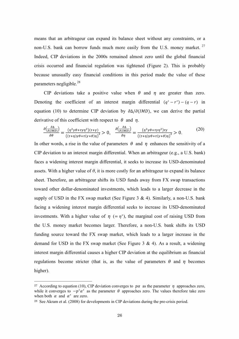
CIP deviations take a positive value when 𝜃 and 𝜂 are greater than zero.
Denoting the coefficient of an interest margin differential (𝑞∗ − 𝑟∗) − (𝑞 − 𝑟) in
equation (10) to determine CIP deviation by 𝜕Δ/𝜕(𝐼𝑀𝐷), we can derive the partial
derivative of this coefficient with respect to 𝜃 and 𝜂.
𝜕(𝜕Δ
𝜕(𝐼𝑀𝐷))
𝜕𝜃=
(𝜂2𝛾𝜃+𝜏𝛾𝜂2)(𝜏+𝛾)
((𝜏+𝜂)𝛾𝜃+𝜏(𝛾+𝜃)𝜂)2 > 0,
𝜕(𝜕Δ
𝜕(𝐼𝑀𝐷))
𝜕𝜂=
(𝜂2𝛾𝜃+𝜏𝛾𝜂2)𝜏𝛾
((𝜏+𝜂)𝛾𝜃+𝜏(𝛾+𝜃)𝜂)2 > 0.
(20)
In other words, a rise in the value of parameters 𝜃 and 𝜂 enhances the sensitivity of a
CIP deviation to an interest margin differential. When an arbitrageur (e.g., a U.S. bank)
faces a widening interest margin differential, it seeks to increase its USD-denominated
assets. With a higher value of θ, it is more costly for an arbitrageur to expand its balance
sheet. Therefore, an arbitrageur shifts its USD funds away from FX swap transactions
toward other dollar-denominated investments, which leads to a larger decrease in the
supply of USD in the FX swap market (See Figure 3 & 4). Similarly, a non-U.S. bank
facing a widening interest margin differential seeks to increase its USD-denominated
investments. With a higher value of 𝜂 (= 𝜂∗), the marginal cost of raising USD from
the U.S. money market becomes larger. Therefore, a non-U.S. bank shifts its USD
funding source toward the FX swap market, which leads to a larger increase in the
demand for USD in the FX swap market (See Figure 3 & 4). As a result, a widening
interest margin differential causes a higher CIP deviation at the equilibrium as financial
regulations become stricter (that is, as the value of parameters 𝜃 and 𝜂 becomes
higher).
27 According to equation (10), CIP deviation converges to 𝑝𝛼 as the parameter 𝜂 approaches zero, while it converges to −𝑝∗𝛼∗ as the parameter 𝜃 approaches zero. The values therefore take zero when both 𝛼 and 𝛼∗ are zero. 28 See Akram et al. (2008) for developments in CIP deviations during the pre-crisis period.

27
We can also derive the relationship regarding how coefficients of liquidity needs
(𝑉, 𝑉∗) vary with the two parameters. Denoting these coefficients by 𝜕Δ/𝜕𝑉 and
𝜕Δ/𝜕𝑉∗ respectively, we can show that the following qualitative relationships hold.
∂(∂Δ
∂𝑉)
∂𝜃,
∂(∂Δ
∂𝑉)
∂𝜂,
∂(∂Δ
∂𝑉∗)
∂𝜃,
∂(∂Δ
∂𝑉∗)
∂𝜂> 0.
(21)
Again, this equation shows that CIP deviations react much more to a change in liquidity
needs when a tighter regulatory reform is implemented.
Note that the extent to which regulatory reforms influence the effect of banks’
default probabilities (𝛼, 𝛼∗) on CIP deviation differs across parameters.
∂(∂Δ
∂𝛼)
∂𝜃,
∂(∂Δ
∂𝛼∗)
∂𝜃> 0, and
∂(∂Δ
∂𝛼)
∂𝜂,
∂(∂Δ
∂𝛼∗)
∂𝜂< 0.
(22)
For example, when the default probability of a non-U.S. bank (𝛼) increases, lenders in
the U.S. money market require a higher premium, which in turn leads the bank to raise
more USD from the FX swap market. With a higher value of θ, an arbitrageur requires a
much larger premium to compensate for the higher marginal cost of dollar funding,
resulting in an even higher CIP deviation. In contrast, with a higher value of 𝜂 (= 𝜂∗), a
non-U.S. bank faces a larger marginal cost in raising USD from the U.S. money market,
and it reduces dollar lending given an interest margin differential. Therefore, the
demand by a non-U.S. bank for USD is suppressed, resulting in a modest rise in CIP
deviation.
Empirical evidence for the impact on CIP deviation
We empirically examine whether the effect of regulatory reforms is reflected in the
change in coefficients of the model. To this end, we estimate Model 1 in equation (12),
using the same monthly series but with different sample periods for the four currency
pairs, and see how the estimated coefficients vary depending on the sample period. We
set the staring period of the sample period to January 2007 and allow the ending point to
differ across examples. Note that the effect of new regulations is expected to appear in
the later stages of the sample period. As explained above, against the backdrop of MMF
reforms, institutional investors have been switching from prime MMFs to government
MMFs since fall 2015. As for the new leverage ratio framework, the public disclosure

28
requirements were introduced in January 2015, and the Volcker rule also took effect in
July 2015.
The upper panels in Figure 8 show the results. The x-axis represents the end of the
sample period. The y-axis represents the estimated coefficients of each explanatory
variable. We can see that the coefficient of interest margin differentials increases
gradually as the ending point of the sample period is extended forward. This observation
is consistent with the model’s prediction in equation (20). That is, the sensitivity of CIP
deviations to interest margin differentials increases with stricter financial regulation (i.e.,
higher θ and 𝜂). In contrast, the estimated coefficients of banks’ default probabilities
(𝛼, 𝛼∗) are stable across the sample periods. This is probably because a rise in the value
of parameters θ and 𝜂 has the opposite effect on the sensitivity of a CIP deviation to
banks’ default probabilities, as shown in equation (22).29
In order to examine whether the change in the coefficients of an interest margin
differential is statistically significant, we estimate Model 1 with a dummy variable
(𝐷𝑈𝑀𝑡𝑇), which takes zero from January 2007 to a point before the period T, and takes
unity from period T to February 2016. Using this variable, we estimate the following
panel equation for i = the euro area, Japan, Switzerland, and the U.K.
Δ𝑖𝑡 = (𝛿𝑇 + 𝛿𝑇𝐷 × 𝐷𝑈𝑀𝑡
𝑇)[(𝑞𝑡∗ − 𝑟𝑡
∗) − (𝑞𝑖𝑡 − 𝑟𝑖𝑡)] + 𝛽𝑇𝛼𝑖𝑡 + 𝛽𝑇∗ 𝛼𝑡
∗ +
𝜆𝑇𝑉𝐼𝑋𝑡 + 𝑐𝑇𝑖 + 휀𝑇𝑖𝑡 ,
where 𝐷𝑈𝑀𝑡𝑇= {
0, 𝑡 < 𝑇
1, 𝑇 ≤ 𝑡 .
(23)
The lower panel of Figure 8 shows the estimation results. The y-axis stands for
estimated coefficients 𝛿𝑇 and 𝛿𝑇𝐷, and the x-axis stands for the period T. Both of the
parameters are positive and statistically significant. While the estimated coefficient
𝛿𝑇 is stable, 𝛿𝑇𝐷 rises as the period T is extended forward. Specifically, the estimation
results suggest that the sensitivity of a CIP deviation to interest margin differentials
becomes higher from around 2014, which corresponds to the period when financial
29 The estimated coefficients of VIX are also stable, although equation (21) suggests that the sensitivity of a CIP deviation to liquidity needs (𝑉, 𝑉∗) rises with higher θ and 𝜂. This may be related to the fact that VIX is an imperfect measure of liquidity needs, as we have discussed.

29
regulations related to the parameters 𝜃 and 𝜂 become stricter. The sensitivity of a CIP
deviation in 2015 is about two times higher than before.
Impact on the liquidity of FX swap markets
Market contacts suggest that regulatory reforms affect not only arbitrage trading
but also market-making by banks in the FX swap market.30 Specifically, some of the
current regulatory reforms have made it difficult for banks to change the size of their
balance sheets flexibly, which has reduced their capacity for market making services,
thereby reducing market liquidity. While our model does not incorporate
market-maker’s activities, we can examine indirectly how the liquidity in the FX swap
market changes.
The importance of market liquidity in CIP deviations is highlighted in several
existing studies, such as Coffey et al. (2009) and Pinnington and Shamloo (2016).
Market liquidity and CIP deviation are considered to interact closely. For example, a
decline in market liquidity may discourage arbitrage trading and market-making activity
by banks, amplifying the widening of CIP deviations.
The upper panel of Figure 9 shows the bid-ask spread for USD/JPY in the Tokyo
FX swap market. The bid-ask spread is a commonly used indicator of market liquidity.
It increased sharply during the middle of the Lehman crisis, then evolved at a low level
for about seven years until it started to rise again in the latter half of 2015, suggesting
that the market has recently become less liquid than before.
As a market-maker in FX swaps, banks borrow USD from other market
participants with a short tenor, typically less than a month, and lend USD with a longer
tenor to borrowers of USD. When the bid-ask spread is high, banks may perceive that
losses are incurred in continuing market making activities, because it is more difficult to
match the needs of market participants. Consequently, banks limit their market-making
activities and reduce the supply of USD in the FX swap market, resulting in a higher
CIP deviation. According to existing studies such as Elliot (2015) and Pinnington and
30 We thank Teppei Nagano (Bank of Japan) for his valuable information on liquidity of the FX swap markets. See also Arai et al. (2016).

30
Shamloo (2016), the bid-ask spreads reflect perceived uncertainty from the market
makers’ perspective in the FX swap market, as well as the cost of executing transactions.
When market makers expect the demand or supply of USD tomorrow will be very
different from that of today, they then raise the bid-ask spread so as to prepare for the
uncertainty, which in turn reduces liquidity in the market.
In order to quantitatively assess the effect of these channels, we run the following
equation for USD/JPY using the EGARCH-in-Mean model.
Δ𝑡 = 𝛿[(𝑞𝑡∗ − 𝑟𝑡
∗) − (𝑞𝑡 − 𝑟𝑡)] + 𝛽𝛼𝑡 + 𝛽∗𝛼𝑡∗ + 𝜆𝑉𝐼𝑋𝑡 + 𝜋𝜎𝑡 + 𝑐 + 𝜖𝑡
𝑙𝑛𝜎𝑡2 = 𝑐𝑜 + 𝑐1 |
𝜖𝑡−1
𝜎𝑡−1| + 𝑐2 (
𝜖𝑡−1
𝜎𝑡−1) + 𝑐3𝑙𝑛𝜎𝑡−1
2 + 𝑐4𝜉𝑡.
(24)
Here, 𝜎𝑡2 is the conditional variance which captures the effect of liquidity of the FX
swap market on CIP deviation. In the conditional variance equation, the variable 𝜉𝑡 is
the liquidity stress of the U.S. money market, which may interact with the liquidity of
the FX swap market.31
Table 6 shows the estimation results. All the estimated coefficients have the correct
sign, and not only the coefficients of interest margin and banks’ default probability, but
the coefficient of conditional standard deviation (𝜎𝑡) is also statistically significant.
Note also that the liquidity shock of the U.S. money market has a statistically significant
impact on the conditional variance (𝜎𝑡2). The upper panel of Figure 9 shows the
estimated conditional standard deviation (𝜎𝑡) together with the bid-ask spread. The
estimated standard deviation (𝜎𝑡) closely tracks the movement of the bid-ask spread,
indicating that the recent decline in market liquidity has contributed to a rise in CIP
deviation.
In order to examine if there is a change in the way that market liquidity affects CIP
deviations, we also estimate the above EGARCH-in-Mean model using different sample
periods. If regulatory reforms influence not only arbitrage trading but also banks’
market-making, there should be a rise in the sensitivity of CIP deviation to both interest
31 The LIBOR-OIS spread can be considered a good indicator of credit risk and liquidity premium. In order to extract liquidity premium from the LIBOR-OIS spread and use it as a proxy of the variable 𝜉𝑡, we regress the USD Libor-OIS spread on the EDF of large U.S. banks (i.e., a proxy of their credit risk). The residual series of the regression is used as the variable 𝜉𝑡.

31
margin differentials and market liquidity (proxied by conditional variance). Similar to
the exercise conducted above, we estimate the model, setting the starting point of the
sample to January 2007 and gradually extending the ending point forward. As shown in
Figure 9, both coefficients of interest margin differential and conditional standard
deviation (𝜎𝑡) increase as the ending point is extended, particularly in 2015 and beyond,
implying that regulatory reform plays a definite role.
4.3. Real money investors as alternative arbitrageurs
While arbitrage trading activities by banks have declined partly due to regulatory
reforms, real money investors, such as asset management companies, sovereign wealth
funds (SWFs) and foreign official reserve managers, have increased their supply of
USD in the FX swap market. For example, market contacts suggest that against the
backdrop of widening CIP deviations, foreign real money investors supply USD through
the FX swap market to invest in JPY-denominated assets. Indeed, foreign investors have
continued to increase their holdings of Japanese Government Bonds in spite of low or
negative yields. In the following, we empirically assess the role of real money investors
in the FX swap market, by assuming that their total AUM is captured by the wealth
endowment of arbitrageurs (𝑊∗) in our model.
Methodology
Based on equations (10) and (11), we first estimate the following equations for
USD/JPY.32
Δ𝑡 = 𝛿1∗(𝑞𝑡
∗ − 𝑟𝑡∗) + 𝛿1(𝑞𝑡 − 𝑟𝑡) + 𝛽1𝛼𝑡 + 𝛽1
∗𝛼𝑡∗ + 𝜆1𝑉𝐼𝑋𝑡 + 𝑐1 + 𝑣1𝑡 (25)
𝑆𝑡 = 𝛿2∗(𝑞𝑡
∗ − 𝑟𝑡∗) + 𝛿2(𝑞𝑡 − 𝑟𝑡) + 𝛽2𝛼𝑡 + 𝛽2
∗𝛼𝑡∗ + 𝜆2𝑉𝐼𝑋𝑡 + 𝑐2 + 𝑣2𝑡 (26)
𝑣1𝑡 and 𝑣2𝑡 are error terms, which represent banks’ liquidity needs (𝑉, 𝑉∗) unexplained
by VIX and the wealth endowment of arbitrageurs (𝑊∗). Note that, as shown in equation
(5), an increase in non-U.S. banks’ liquidity needs (𝑉) means a rightward shift in the
demand curve for USD through the FX swap market, which leads to an increase in both
32 The monthly volume of FX swap transaction (𝑆) is available only for USD/JPY. We use the daily average turnover of FX swaps traded by foreign exchange brokers in Tokyo in each month.
32
CIP deviation (Δ) and the transaction volume of FX swap (S). In contrast, as shown in
equation (9), an increase in arbitrageurs’ liquidity needs (𝑉∗) or a decrease in their
wealth endowment (𝑊∗) means a leftward shift in the supply curve for USD through the
FX swap market, which leads to an increase in CIP deviation (Δ) and a decrease in the
transaction volume of FX swap (𝑆).
By making use of these characteristics and applying the VAR identification scheme
with sign restrictions, we next decompose the error terms into two components: (i)
demand shock related to non-U.S. banks’ liquidity needs, and (ii) supply shock related to
arbitrageurs’ liquidity needs and wealth endowment.33 That is, we assume that the error
terms 𝑣1𝑡 and 𝑣2𝑡 are expressed by a linear combination of two structural shocks in
the VAR model, and identify demand shock and supply shock by making use of sign
restrictions.
Estimation results
The upper panel in Figure 10 shows the time paths of two estimated structural
shocks for USD/JPY. The middle panels show the decomposition of a CIP deviation and
swap transaction volume into interest margin differential, banks’ EDFs, VIX, and two
structural shocks based on the model.34 Both demand and supply shocks have been an
important source of variations in CIP deviation Δ and transaction volume S. Demand
shock affected CIP deviation Δ and the transaction volume S positively in the latter half
of 2015 and beyond. While supply shock lowered CIP deviation Δ and boosted the
transaction volume S in 2012 and 2013, the sign of the shock’s effects was flipped in the
middle of 2014, increasing CIP deviation Δ and lowering the transaction volume S.
As regards supply shock, we are unable to disentangle the contributions of 𝑉∗ and
33 In order to estimate demand and supply shocks from residual series 𝑣1𝑡 and 𝑣2𝑡 , we first formulate the vector autoregression (VAR) that consists of these two residual series, and then extract demand and supply shocks from error terms of this VAR by imposing two restrictions. The first restriction is that a positive demand shock contemporaneously increases 𝑣1𝑡 and 𝑣2𝑡, and the second restriction is that a positive supply shock contemporaneously increases 𝑣1𝑡 and decreases 𝑣2𝑡. See Uhlig (2005) for details of VAR identification with sign restrictions. 34 The contribution of demand shocks and supply shocks can be obtained as the linear combination of a sequence of these shocks based on the VAR model.
33
𝑊∗, and only able to discuss the combined role played by liquidity needs of arbitrageurs
and their wealth endowment. However, what we observe from the lower panel of Figure
10 is the presence of the sovereign wealth funds (SWFs) of oil-producing countries in
the FX swap market. This panel shows that the correlation with oil price is negative for
the impact of supply shock on CIP deviation, and positive for that on FX swap
transaction volume. In addition, for both CIP deviation and FX swap transaction volume,
the absolute values of the correlation coefficients are recently larger than before,
indicating that the relationship between supply shock and oil price has become strong.
Market contacts indicate that SWFs in oil-producing countries have supplied USD in
the FX swap market. This seems to hold true especially in the period from 2011 to the
middle of 2014 when oil prices were fairly high, which implies an increase in the wealth
endowment (𝑊∗) of SWFs and hence the leftward shift of the supply curve of USD
through the FX swap market. Indeed, in this period, supply shocks tend to be negative
(Figure 10 (1)), and they contribute to a decline in CIP deviation and an increase in FX
swap transaction volume (Figure 10 (2)).
However, market contacts say that since oil prices plummeted in 2015, the SWFs
that had formerly allocated their oil money in USD to the FX swap market have started
to withdraw from the market. Such a development should appear as a negative shock
in 𝑊∗, which would cause a leftward shift in the supply curve of USD through the FX
swap market. Indeed, from mid-2014, supply shocks tend to be positive (Figure 10 (1)),
and they contribute to an increase in CIP deviation and a decline in FX swap transaction
volume (Figure 10 (2)). Because statistics are not available on the portfolio of real
money investors, such as SWFs and foreign official reserves, we cannot show direct
evidence of their impact on the FX swap market. However, other market contacts
indicate that during the period of emerging market currency depreciation in mid-2015,
official reserve managers shifted their USD-denominated assets from less liquid
cross-currency funding markets to US Treasury bills, driven by their increased need to
intervene in the FX markets to support their home-currency.35 Again, such a change in
35 According to US Treasury (2016), in the latter half of 2015, many emerging market central banks responded to capital outflows by intervening in FX markets to defend their currencies, and the

34
real money investors’ portfolios is reflected in supply shock, i.e. a decline in
arbitrageurs’ wealth endowment (𝑊∗) in our model.
It should be also noted that stricter financial regulations (i.e., higher 𝜃 and 𝜂 in
our model) increases the sensitivity of CIP deviations to wealth endowment shocks.
That is, from equation (10), the following qualitative relationships hold.
∂(∂Δ
∂𝑊∗)
∂𝜃,
∂(∂Δ
∂𝑊∗)
∂𝜂< 0.
(27)
When real money investors face a fall in total AUM (𝑊∗) and reduce the supply of USD
in the FX swap market, the demand-supply balance of USD tightens, leading to an
increase in CIP deviation. With a higher value of 𝜂, a non-U.S. bank faces a higher
marginal cost for funding USD from the U.S. money market, and becomes less
responsive to changes in CIP deviation. That is, the demand curve of USD in the FX
swap market becomes steeper, as shown in equation (5). Consequently, the fall in supply
of USD is more easily translated into an even higher CIP deviation. Similarly, with a
higher value of θ, a U.S. bank requires a much larger premium to compensate for the
higher funding costs, which implies that the supply curve of USD in the FX swap
market becomes steeper, as shown in equation (9). Again, the leftward shift of the
steeper supply curve leads to a much higher CIP deviation. In this sense, an adverse
shock in the asset management sector, such as a fall in the AUM of real money investors,
is amplified by stricter financial regulations.
4.4. Implications for financial stability
Historically, non-U.S. bank’s creditworthiness has largely affected their overseas
dollar lending and financial stability through variations in CIP deviation. During both
Japan’s banking crisis in the late 1990s and the eurozone sovereign debt crisis in 2011,
an increase in CIP deviation brought about by a worsening of banks’ creditworthiness
was followed by a cut in overseas lending extended by non-U.S. banks. In the former
crisis, as Peek and Rosengren (2001, 2002) document, because of the deterioration in
their balance sheet conditions and an increase in the dollar funding premium (the
intervention caused central banks to dip into their stocks of foreign exchange reserves.

35
so-called “Japan premium”), Japanese banks cut lending, in particular wholesale lending
to the U.S. As for the latter crisis, Ivashina et al. (2015) document that eurozone banks
cut their dollar lending more than their euro lending. The impact of non-U.S. banks’
creditworthiness on the dollar funding premium and their dollar lending in cases such as
these is well described in our model. Differentiating equations (6) and (10) with respect
to non-U.S. banks’ default probability (𝛼) yields the following relationships:
∂Δ
∂𝛼> 0, and 𝜕𝐿𝑈𝑆
𝜕𝛼< 0. (28)
In recent years, however, the linkage between banks’ creditworthiness and CIP
deviation has been weakened. One possible reason behind the diminishing impact of
banks’ creditworthiness is advances in regulatory reforms, such as revised capital
requirements based on the Basel Accords. Instead of banks’ creditworthiness, interest
margin differentials due to diverging monetary stances have a larger impact on the
dollar funding premium, as explained in Section 4.1. This then begs the question, how
does monetary policy divergence, especially resulting from changes in the Fed’s policy
stance, affect non-U.S. financial institutions’ lending and investing behavior? Although
a rise in the U.S. interest margin (𝑞∗ − 𝑟∗) encourages non-U.S. financial institutions to
“search for yield” on USD-denominated assets (i.e., 𝜕𝐿𝑈𝑆
𝜕(𝑞∗−𝑟∗)> 0), our model suggests that
regulatory reforms limit the impact of U.S. monetary policy on their activities. That is,
the following qualitative relationships hold.36
𝜕(𝜕𝐿𝑈𝑆
𝜕(𝑞∗−𝑟∗))
𝜕𝜃,
𝜕(𝜕𝐿𝑈𝑆
𝜕(𝑞∗−𝑟∗))
𝜕𝜂< 0 .
(29)
Because regulatory reforms (i.e., higher 𝜃 and 𝜂 in our model) raise the marginal
costs of USD funding and increase the sensitivity of CIP deviations to interest margin
differentials (see equation (20)), such reforms dampen the impact of a rise in the U.S.
interest margin (𝑞∗ − 𝑟∗) on non-U.S. financial institutions’ lending and investments
(𝐿𝑈𝑆) and prevent them from engaging in excessive “search for yield” activities. This
36 Unlike CIP deviation Δ in equation (10), USD-denominated loan 𝐿𝑈𝑆 in equation (6) cannot be expressed as a function of an interest margin differential. We therefore derive a change in USD-denominated loans 𝐿𝑈𝑆 only with respect to a change in interest margin in USD. It should also be noted that similar to the discussion in Section 2, we maintain the assumption that 𝛾𝜂 > 𝜃𝜏 here.

36
then helps the U.S. monetary authorities avoid financial imbalances like Alan
Greenspan’s “bond conundrum,” and contributes to global financial stability.37
It should be noted, however, that the regulatory reforms bring about dual impacts
on the global financial system. Although stricter regulations (i.e., higher 𝜃 and 𝜂 in
our model) limit the impact of monetary policy divergence on non-U.S. financial
institutions’ “search for yield” activities, they amplify the impact of liquidity shortage of
banks and wealth shocks facing arbitrageurs. Namely, we can derive the following
qualitative relationships from equations (6) and (10).
𝜕(𝜕𝐿𝑈𝑆
𝜕𝑉)
𝜕𝜃,
𝜕(𝜕𝐿𝑈𝑆
𝜕𝑉)
𝜕𝜂,
𝜕(𝜕𝐿𝑈𝑆𝜕𝑉∗ )
𝜕𝜃,
𝜕(𝜕𝐿𝑈𝑆𝜕𝑉∗ )
𝜕𝜂< 0, and
𝜕(𝜕𝐿𝑈𝑆𝜕𝑊∗ )
𝜕𝜃,
𝜕(𝜕𝐿𝑈𝑆𝜕𝑊∗ )
𝜕𝜂> 0.
(30)
An increase in banks’ liquidity needs and a decline in the total AUM of real money
investors leads to a tightening of demand-supply balance in the FX swap market and a
higher dollar funding premium. This effect is amplified by stricter regulations which
increase the marginal costs of dollar funding for banks. As a result, given interest
margin differentials, non-U.S. financial institutions further reduce their
USD-denominated investments. If their investments are cut rapidly and on a large scale,
this may destabilize the global financial system.
Although financial regulations, such as LCR and NSFR, contribute to reducing the
risk of liquidity shortage for global banks, there remains the risk of adverse shocks in
the asset management sector, whose presence in the FX swap market has increased
recently. Our model suggests that the impact of severely adverse shocks in the asset
management sector, such as a sharp fall in the AUM of real money investors, are
amplified by stricter financial regulations (i.e., higher 𝜃 and 𝜂) and transmitted to
the FX swap market and beyond, inducing non-U.S. banks to further cut back on their
USD-denominated lending. This then feeds back into the asset management sector by
driving down asset prices and thereby having a further negative impact on the real
money investors’ AUM.
37 See, for instance, King (2006) for a discussion of the conundrum.
37
5. Conclusion
In this paper, we study the determinants of CIP deviations and outline the
implications for monetary policy divergence and financial stability. First, we
theoretically show that CIP deviation is driven by several factors: interest margin
differentials, banks’ default probabilities, banks’ liquidity needs, and the wealth
endowment of arbitrageurs. We then empirically show that our model’s predictions are
consistent with the data. In addition, we find that in recent years the key driver of CIP
deviation has changed from banks’ default probabilities to interest margin differentials.
Given that interest margin is largely affected by the monetary policy stance, this result
suggests the growing importance of monetary policy divergence in the FX swap market.
We also discuss the impact of regulatory reforms on the FX swap market and
non-U.S. banks’ lending and investing behavior. While stricter regulations limit non-U.S.
banks’ excessive “search for yield” activities resulting from monetary policy divergence,
they amplify the impact of adverse shocks in the asset management sector on the dollar
funding market and hence non-U.S. banks’ dollar lending. Both these positive and
negative effects of regulatory reforms are attributable to an increase in the marginal cost
of banks’ dollar funding. We have pointed out that the latter negative (and unintended)
effect of regulations has become potentially larger due to changes in the cross-currency
market structure, particularly in the type of arbitragers as USD liquidity providers.
While arbitrage trading by banks has declined due to regulatory reforms, real money
investors have come to play a greater role in the supply of USD in the FX swap market.
However, as in 2015 when emerging market currencies depreciated and oil prices
declined, real money investors such as foreign official reserve managers and SWFs are
not stable or reliable USD liquidity providers. When a severely adverse shock occurs in
the global financial system, real money investors, as well as U.S. banks, may sell off
their USD-denominated assets and/or reduce the supply of USD to non-U.S. financial
institutions in the FX swap market. This then induces non-U.S. financial institutions to
cut their USD-denominated assets, which may amplify the sale of financial assets by
real money investors. It is therefore important to seek measures that minimize the

38
unintended negative effects of financial regulations without compromising their positive
effect.38
38 Financial Stability Board (2016) proposes policy recommendations to address structural vulnerabilities from asset management activities. These policies are expected to help reduce the risk of adverse shocks in the asset management sector.
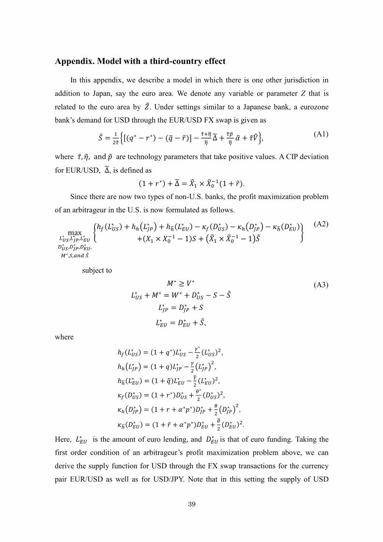
39
Appendix. Model with a third-country effect
In this appendix, we describe a model in which there is one other jurisdiction in
addition to Japan, say the euro area. We denote any variable or parameter Z that is
related to the euro area by �̃�. Under settings similar to a Japanese bank, a eurozone
bank’s demand for USD through the EUR/USD FX swap is given as
�̃� =1
2�̃�{[(𝑞∗ − 𝑟∗) − (�̃� − �̃�)] −
�̃�+�̃�
�̃�Δ̃ +
�̃��̃�
�̃��̃� + �̃��̃�}, (A1)
where �̃�, �̃�, and 𝑝 are technology parameters that take positive values. A CIP deviation
for EUR/USD, Δ̃, is defined as
(1 + 𝑟∗) + Δ̃ = �̃�1 × �̃�0−1(1 + �̃�).
Since there are now two types of non-U.S. banks, the profit maximization problem
of an arbitrageur in the U.S. is now formulated as follows.
max𝐿𝑈𝑆
∗ ,𝐿𝐽𝑃∗ ,𝐿𝐸𝑈
∗
𝐷𝑈𝑆∗ ,𝐷𝐽𝑃
∗ ,𝐷𝐸𝑈∗ ,
𝑀∗,𝑆,𝑎𝑛𝑑 �̃�
{ℎ𝑓(𝐿𝑈𝑆
∗ ) + ℎℎ(𝐿𝐽𝑃∗ ) + ℎℎ̃(𝐿𝐸𝑈
∗ ) − 𝜅𝑓(𝐷𝑈𝑆∗ ) − 𝜅ℎ(𝐷𝐽𝑃
∗ ) − 𝜅ℎ̃(𝐷𝐸𝑈∗ )
+(𝑋1 × 𝑋0−1 − 1)𝑆 + (�̃�1 × �̃�0
−1 − 1)�̃�}
(A2)
subject to
𝑀∗ ≥ 𝑉∗
𝐿𝑈𝑆∗ + 𝑀∗ = 𝑊∗ + 𝐷𝑈𝑆
∗ − 𝑆 − �̃� 𝐿𝐽𝑃
∗ = 𝐷𝐽𝑃∗ + 𝑆
𝐿𝐸𝑈∗ = 𝐷𝐸𝑈
∗ + �̃�,
(A3)
where
ℎ𝑓(𝐿𝑈𝑆∗ ) = (1 + 𝑞∗)𝐿𝑈𝑆
∗ −𝛾∗
2(𝐿𝑈𝑆
∗ )2,
ℎℎ(𝐿𝐽𝑃∗ ) = (1 + 𝑞)𝐿𝐽𝑃
∗ −𝛾
2(𝐿𝐽𝑃
∗ )2,
ℎℎ̃(𝐿𝐸𝑈∗ ) = (1 + �̃�)𝐿𝐸𝑈
∗ −�̃�
2(𝐿𝐸𝑈
∗ )2,
𝜅𝑓(𝐷𝑈𝑆∗ ) = (1 + 𝑟∗)𝐷𝑈𝑆
∗ +𝜃∗
2(𝐷𝑈𝑆
∗ )2,
𝜅ℎ(𝐷𝐽𝑃∗ ) = (1 + 𝑟 + 𝛼∗𝑝∗)𝐷𝐽𝑃
∗ +𝜃
2(𝐷𝐽𝑃
∗ )2,
𝜅ℎ̃(𝐷𝐸𝑈∗ ) = (1 + �̃� + 𝛼∗𝑝∗)𝐷𝐸𝑈
∗ +�̃�
2(𝐷𝐸𝑈
∗ )2.
Here, 𝐿𝐸𝑈 ∗ is the amount of euro lending, and 𝐷𝐸𝑈
∗ is that of euro funding. Taking the
first order condition of an arbitrageur’s profit maximization problem above, we can
derive the supply function for USD through the FX swap transactions for the currency
pair EUR/USD as well as for USD/JPY. Note that in this setting the supply of USD

40
through the EUR/USD FX swap and that through the USD/JPY FX swap are
interrelated. Namely, the supply for USD through the USD/JPY FX swap, denoted as 𝑆,
is expressed as follows:
𝑆 = 𝜓𝑞∗−𝑟∗(𝑞∗ − 𝑟∗) + 𝜓𝑞−𝑟(𝑞 − 𝑟) + 𝜓�̃�−�̃�(�̃� − �̃�) + 𝜓𝛼∗ 𝛼∗ + 𝜓Δ Δ +
𝜓Δ̃Δ̃ + 𝜓𝑉∗−𝑊∗(𝑉∗ − 𝑊∗),
(A4)
where coefficient 𝜓𝑧 that is attached to a variable 𝑍 is given as the combination of
parameters 𝜃 , 𝜃∗, �̃�, 𝛾, 𝛾∗, �̃�, 𝑝∗. Assuming that 𝛾 = 𝛾∗ = �̃� and 𝜃 = 𝜃∗ = �̃�, the signs
of these coefficients can be determined such that 𝜓𝑞∗−𝑟∗ , 𝜓�̃�−�̃�, 𝜓𝑉∗−𝑊∗ , 𝜓�̃� < 0 and
𝜓𝑞−𝑟 , 𝜓𝛼∗ , 𝜓𝛥 > 0. The symmetric equation holds for USD supply of an arbitrageur to
Eurozone banks, which is
�̃� = 𝜙𝑞∗−𝑟∗(𝑞∗ − 𝑟∗) + 𝜙𝑞−𝑟(𝑞 − 𝑟) + 𝜙�̃�−�̃�(�̃� − �̃�) + 𝜙𝛼∗ 𝛼∗ + 𝜙Δ Δ +
𝜙Δ̃Δ̃ + 𝜙𝑉∗−𝑊∗(𝑉∗ − 𝑊∗),
(A5)
where coefficient 𝜙𝑧 that is attached to a variable 𝑍 is given as the combination of
parameters 𝜃, 𝜃∗, �̃�, 𝛾, 𝛾∗, �̃�, 𝑝∗. Assuming the same conditions for the parameters, the
signs of these coefficients can be determined again, such that
𝜙𝑞∗−𝑟∗ , 𝜙𝑞−𝑟 , 𝜙𝑉∗−𝑊∗ , 𝜙𝛥 < 0 and that 𝜙�̃�−�̃� , 𝜙𝛼∗ , 𝜙�̃� > 0.
Using equations (5), (A1), (A4), and (A5), the CIP deviation for USD/JPY at the
equilibrium is expressed as follows.
Δ = 𝜌𝑞∗−𝑟∗(𝑞∗ − 𝑟∗) + 𝜌𝑞−𝑟(𝑞 − 𝑟) + 𝜌�̃�−�̃�(�̃� − �̃�) + 𝜌𝛼∗𝛼∗ + 𝜌𝛼𝛼 + 𝜌𝛼 ̃�̃�
+ 𝜌𝑉∗𝑉∗ + 𝜌𝑉𝑉 + 𝜌�̃��̃� + 𝜌𝑊∗𝑊∗
(A6)
Coefficient 𝜌𝑧 that is attached to a variable 𝑍 is given as the combination of
technology parameters. It can be shown that under the symmetric assumption about the
parameter values, their signs are pinned down such that 𝜌𝑞−𝑟, 𝜌�̃�−�̃�, 𝜌𝛼∗ , 𝜌𝑊∗ < 0 and
𝜌𝑞∗−𝑟∗ , 𝜌𝛼 , 𝜌�̃� , 𝜌𝑉 , 𝜌𝑉∗ , 𝜌�̃� > 0. 39
It is seen from equation (A6) that CIP deviation Δ of USD/JPY is now influenced
not only by the interest rate margin in Japan, together with the Japanese bank’s default
probability and its liquidity needs but also by those associated with the euro area. For
instance, other things being equal, a widening interest margin in the euro area reduces
the demand for USD by Eurozone banks, which then increases USD available for
39 We assume, similar to discussion in Section 2, that inequality 𝜂𝛾 > 𝜃𝜏 holds here.

41
Japanese banks in the FX swap market. Consequently, CIP deviation falls.

42
Reference
Akram, Q. F., D. Rime, and L. Sarno (2008) "Arbitrage in the Foreign Exchange Market: Turning on the Microscope," Journal of International Economics, vol.76, pp. 237-253.
Aoki, K., and N. Sudo (2013) "Bank’s regulation, asset portfolio choice of banks, and macroeconomic dynamics," CARF F-Series CARF-F-323, Center for Advanced Research in Finance, Faculty of Economics, The University of Tokyo.
Arai, T., Y. Makabe, Y. Ookawara, and T. Nagano (2016) "Recent trends in cross-currency basis," Bank of Japan Review Series, forthcoming.
Avdjiev, S., and E. Takats (2016) "Monetary policy spillovers and currency networks in cross-border bank lending," BIS Working Papers, 549.
Baba, N., and F. Packer (2009a) "Interpreting Deviations from Covered Interest Parity During the Financial Market Turmoil of 2007--08," Journal of Banking & Finance vol. 33, pp. 1953-1962
Baba, N., and F. Packer (2009b) "From Turmoil to Crisis: Dislocations in the FX Swap Market Before and After the Failure of Lehman Brothers," BIS Working Papers, No 285.
Baba, N., F. Packer, and T. Nagano (2008) "The spillover of Money Market Turbulence to FX Swap and Cross-Currency Swap Markets," BIS Quarterly Review, pp. 73-86.
Bank of Japan (2016) "Financial System Report," April. Borio, C., L. Gambacorta, and B. Hofmann (2015) "The Influence of Monetary Policy on
Bank Profitability," BIS Working Paper, No. 514. Borio, C., R. McCauley, P. McGuire, and V. Sushko (2016) "Whatever happened to covered
interest parity? Hedging demand meets limits to arbitrage," forthcoming. Coffey, N., W. B. Hrung, and A. Sarkar (2009) "Capital Constraints, Counterparty Risk, and
Deviations from Covered Interest Rate Parity," Federal Reserve Bank of New York Staff Reports, No. 393.
Elliott, D. J. (2015) "Market liquidity: A primer," Brookings Institution. Financial Stability Board (2016) "Consultative Document, Proposed Policy
Recommendations to Address Structural Vulnerabilities from Asset Management Activities."
Gambacorta, L., B. Hofmann, and G. Peersman (2014) "The Effectiveness of Unconventional Monetary Policy at the Zero Lower Bound: A Cross-Country Analysis," Journal of Money, Credit and Banking, vol. 46, pp. 615-642.
He, D., E. Wong, A. Tsang, and K. Ho (2015) "Asynchronous Monetary Policies and International Dollar Credit," HKIMA Working Paper No. 19/2015.
Ivashina, V., D. S. Scharfstein, and J. C. Stein (2015) "Dollar Funding and the Lending Behaviour of Global Banks," Quarterly Journal of Economics vol. 130, pp. 1241-1281.
Kimura, T. and J. Nakajima (2016) "Identifying conventional and unconventional monetary policy shocks: a latent threshold approach," The B.E. Journal of Macroeconomics, vol. 16, pp. 277-300.
King, M. A. (2006) "The Governor’s speech in Ashford, Kent," Bank of England
43
Quarterly Bulletin, pp. 80-82. McGuire, P., and G. von Peter (2009) "The US Dollar Shortage in Global Banking," BIS
Quarterly Review, pp. 47-63. Peek, J., and E. S. Rosengren (2001) " Determinants of the Japan premium: actions speak
louder than words," Journal of International Economics, vol. 53, pp. 283-305. Peek, J., and E. S. Rosengren (2002) "Japanese Banking Problems: Implications for
Southeast Asia," Banking, Financial Integration, and International Crises, vol. 3, chapter 10, pp. 303-332.
Pinnington, J., and M. Shamloo (2016) "Limits to Arbitrage and Deviations from Covered Interest Rate Parity," Bank of Canada Staff Discussion Paper.
Rogers, J. H., C. Scotti, and J. Wright (2014) "Evaluating Asset-Market Effects of Unconventional Monetary Policy: A Cross-Country Comparison," International Finance Discussion Papers 1101, Board of Governors of the Federal Reserve System (U.S.).
Shin, H. S. (2016) "Global Liquidity and Procyclicality," Speech at World Bank Conference “The State of Economics, The State of the World”.
Terajima, Y., H. Vikstedt, and J. Witmer (2010) "The Impact of the Financial Crisis on Cross-Border Funding," Bank of Canada Financial System Review, pp. 33-40.
Uhlig, H. (2005) "What are the effects of monetary policy on output? Results from an agnostic identification procedure," Journal of Monetary Economics, vol. 52, pp. 381-419.
U.S. Department of the Treasury (2016) "Foreign Exchange Policies of Major Trading Partners of the United States."

Note:
Source:
Figure 1: USD-denominated foreign position of banks
“Non-U.S. banks’ USD-denominated foreign claims” and “Non-U.S. banks’ USD-denominatedforeign liabilities” are calculated as USD-denominated foreign claims and liabilities of all countriesminus those of U.S. banks, respectively. “Non-U.S. banks’ cross currency funding (i.e., FX swap)”is defined as “Non-U.S. banks’ USD-denominated foreign claims” minus “Non-U.S. banks’ USD-denominated foreign liabilities.” See McGuire and von Peter (2009) on how to calculate the USDposition of banks using BIS international banking statistics.
BIS consolidated banking statistics (immediate borrower basis); BIS locational banking statistics bynationality.
4
6
8
10
12
14
16
0
4
8
12
16
20
24
CY2000 01 02 03 04 05 06 07 08 09 10 11 12 13 14 15
U.S. banks’ USD-denominated foreign claims (lhs)
Non-U.S. banks’ USD-denominated foreign claims (lhs)
Non-U.S. banks’ USD-denominated foreign liabilities (lhs)
Non-U.S. banks’ cross currency funding ratio (rhs)
tril. USD %
①
②
① −②
①

(1) CIP deviation (3M)
(2) Banks’ default probability
Notes: 1.
2. CIP deviation is calculated as FX swap-implied dollar rates minus USD Libor. 3.
4. “Japan Premium” is calculated as 3-month USD TIBOR minus 3-month USD LIBOR. Source: Bloomberg; Moody’s; BOJ.
The shaded areas correspond to the period of Japan’s financial crisis (November 1997 throughJanuary 1999) , the global financial crisis (December 2007 through June 2009), and the eurozonesovereign debt crisis (May 2011 through June 2012).
Figure 2: CIP deviation and banks’default probability
The average of the Expected Default Frequency (EDF) of the GSIBs, which are headquartered ineach country, is used as the measure of banks’ default probability. For the euro area, the average ofthe EDF of the GSIBs in France, Germany, and Italy is used.
-0.8-0.6-0.4-0.20.00.20.40.60.81.01.21.41.6
CY1995 2000 2005 2010 2015
EUR/USD USD/JPY
%
0.0
0.2
0.4
0.6
0.8
1.0
1.2
0
1
2
3
4
5
6
7
CY1995 2000 2005 2010 2015EDF of banks in Japan (lhs)EDF of banks in the euro area (lhs)Japan Premium (rhs)
% %pts
-0.8-0.6-0.4-0.20.00.20.40.60.81.01.21.41.6
CY1995 2000 2005 2010 2015
USD/CHF GBP/USD
%
0
1
2
3
4
5
6
7
CY1995 2000 2005 2010 2015EDF of banks in the U.S.EDF of banks in SwitzerlandEDF of banks in the U.K.
%

(Assets) (Liabilities)
(Assets) (Liabilities)
Note: The figures in parentheses are the interest rates applied to each asset or liability.
Japanese banks (Non-U.S. financial institutions)U
SDde
nom
inat
edJP
Yde
nom
inat
ed
Figure 3: Balance sheets of global banks in the model economy
JPY
deno
min
ated
USD
deno
min
ated
USD
deno
min
ated
JPY
deno
min
ated
USD
deno
min
ated
JPY
deno
min
ated
U.S. banks and other arbitrageurs
(𝑟∗ + 𝛼𝑝)
(𝑞∗)
(0)
(q) (r)
𝐿𝑈𝑆
𝑀
𝐿𝐽𝑃 𝐷𝐽𝑃
𝐷𝑈𝑆
𝑆 (𝑟∗ − 𝑟 + Δ)
(𝑟∗)
(𝑞∗)
(0)
(q)
𝐿𝑈𝑆∗
𝑀∗
𝐿𝐽𝑃∗
𝐷𝐽𝑃∗
𝐷𝑈𝑆∗
𝑊∗
(𝑟 + 𝛼∗𝑝∗)
𝑆 (𝑟∗ − 𝑟 + Δ)

Flow of USDFlow of JPY
Note: The figures in parentheses are the interest rates applied to each asset or liability.
JPY fundingand deposit markets
JPY bondand loan markets
U.S. banks andother arbitrageurs
Japanese banks(Non-US financial
institutions)
Figure 4: Flow of funds in the model economy
USD bondand loan markets
USD fundingand deposit markets
FX swap market
𝐿𝑈𝑆 (𝑞∗)
𝐿𝑈𝑆∗
(𝑞∗)
𝐷𝑈𝑆 (𝑟∗ + 𝛼𝑝)
𝐷𝑈𝑆∗
(𝑟∗)
(𝑟∗ − 𝑟 + Δ)
𝑆 𝑆
(𝑟∗ − 𝑟 + Δ)
𝐷𝐽𝑃
(𝑟)
𝐷𝐽𝑃∗
(𝑟 + 𝛼∗𝑝∗)
𝐿𝐽𝑃
(𝑞)
𝐿𝐽𝑃∗
(𝑞)
FED (Monetary policy)
Borrowers
Borrowers
BOJ (Monetary policy)
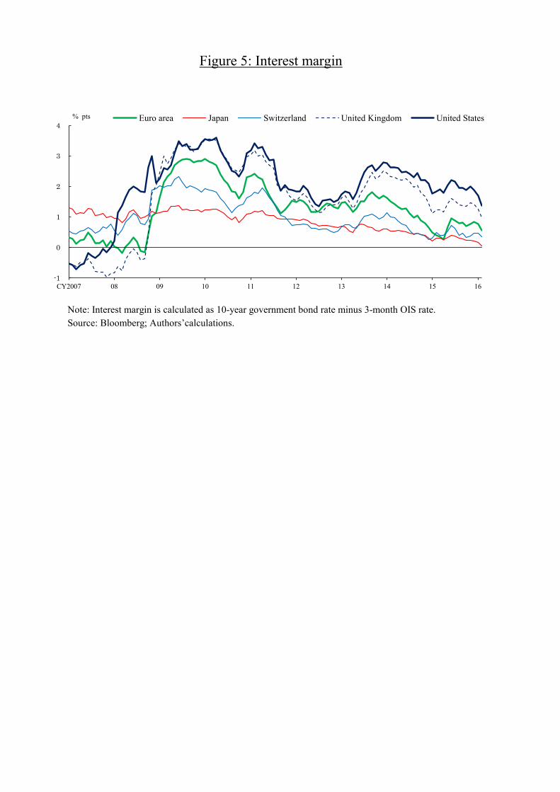
Note: Interest margin is calculated as 10-year government bond rate minus 3-month OIS rate. Source: Bloomberg; Authors’calculations.
Figure 5: Interest margin
-1
0
1
2
3
4
CY2007 08 09 10 11 12 13 14 15 16
Euro area Japan Switzerland United Kingdom United States% pts

(1) EUR/USD (2) USD/JPY
(3) USD/CHF (4) GBP/USD
Notes: 1.
2.
Figure 6: Decomposition of CIP deviation
Each panel shows the quarterly average of the decomposition of a CIP deviation based on theregression results of Model 3 shown in table 5. Contributions of constant terms are not depicted.“Central banks’ balance sheet” in each panel is the contribution of the difference in growth rates ofthe central banks’ balance sheets. “EDF” in each panel is the sum of the contribution of EDF in thenon-U.S. jurisdiction and EDF in the U.S., indicating the net effect of banks’ default probabilities.Residuals in each panel include the contribution of control variables.
-0.6
-0.4
-0.2
0.0
0.2
0.4
0.6
CY2008 10 12 14 16
%
-0.8
-0.6
-0.4
-0.2
0.0
0.2
0.4
0.6
0.8
CY2008 10 12 14 16
%
-0.4
-0.2
0.0
0.2
0.4
0.6
0.8
CY2008 10 12 14 16
%
-0.4
-0.2
0.0
0.2
0.4
0.6
0.8
1.0
CY2008 10 12 14 16
Central banks’ balance sheet EDFVIXResidualCIP deviation
%

Notes: 1.
2.
Source: Investment Company Institute.
Figure 7: MMF total assets
Government MMFs are defined as MMFs that invest 99.5% or more of their total assets in cash, governmentsecurities, and/or government repurchase agreements. Prime MMFs are defined as MMFs that primarilyinvest in corporate debt securities.The vertical line corresponds to the compliance date for amendments related to MMF reforms released by theSecurities and Exchange Commission (October 2016).
0
1
2
3
07 08 09 10 11 12 13 14 15 16
Prime MMFs Government MMFstril. USD
CY2007

(1) Coefficients estimated based on different sample periods(a) Interest margin differential (b) US banks’ EDF
(c) Non-US banks’ EDF (d) VIX
(2) Coefficients of interest margin differential based on the dummy-variable approach(a) Interest margin differential (b) DUM × Interest margin differential
Notes: 1.
2.
Figure 8: Estimated effects of regulatory reforms
For panels (2), the x-axis denotes the starting period from which the dummy variable takes unity.Dotted lines indicate 95 percent confidence intervals.
For panels (1), the x-axis denotes the end of the sample period used to estimate the coefficient ofthe variable, which is depicted in the y-axis. Dotted lines indicate 95 percent confidence intervals.
-0.05
0.00
0.05
0.10
0.15
0.20
CY2012 13 14 15
0.00
0.02
0.04
0.06
0.08
CY2012 13 14 15 16
0.00
0.05
0.10
0.15
0.20
CY2012 13 14 15 16
-0.10
-0.08
-0.06
-0.04
-0.02
0.00
CY2012 13 14 15 16
0.00
0.01
0.02
0.03
CY2012 13 14 15 16
End of sample period
-0.05
0.00
0.05
0.10
0.15
0.20
CY2012 13 14 15
End of sample period
End of sample period End of sample period
𝛿𝑇
𝑇 𝑇
𝛿𝑇𝐷

(1) Bid-ask spread of FX forwards (3M) and conditional standard deviation estimated by EGARCH model
(2) Coefficients of explanatory variables in EGARCH model(a) Conditional standard deviation (b) Interest margin differential
Note:
Source: Bloomberg; BOJ; Authors’ calculations.
Figure 9: Effects of market liquidity on CIP deviation
For panels (2), the x-axis denotes the end of the sample period used to estimate the coefficient ofthe variable, which is depicted in the y-axis. Dotted lines indicate 95 percent confidence intervals.
0.0
0.2
0.4
0.6
0.8
0
2
4
6
8
CY2007 08 09 10 11 12 13 14 15 16
Bid-ask spread (lhs) Conditional standard deviation (rhs)pips
-4
-2
0
2
4
6
8
CY2012 13 14 15 160.00
0.02
0.04
0.06
0.08
0.10
CY2012 13 14 15 16End of sample period End of sample period
𝜎𝑡 𝑞𝑡∗ − 𝑟𝑡
∗ − 𝑞𝑡 − 𝑟𝑡

(1) Demand and supply shocks
(2) Decomposition of CIP deviation and FX swap transaction volume(a) CIP deviation (b) FX swap transaction volume
(3) Relationship between oil price and the impact of supply shocks
Notes: 1. 2.
3.
Source: Bloomberg; Authors’calculations.
Figure 10: Decomposition of CIP deviation and FX swap transaction volume (USD/JPY)
For panel (3), figures in parenthesis are correlation coefficients. We use WTI (West TexasIntermediate) as the measure of oil price.
The middle panel shows the quarterly average of the decomposition of CIP deviation and FX swaptransaction based on the estimation results. Note that contributions of constant terms are notdepicted. “Interest margin differential” and “EDF” in each panel are the sum of the contribution ofinterest margin in Japan and in the U.S., and the sum of the contribution of EDF in Japan and theU.S., respectively. “FX swap transaction volume” is the log deviation of the volume from its averagein 2006.
The size of demand and supply shocks is normalized so that its variance is unity.
-0.4
-0.3
-0.2
-0.1
0.0
0.1
0.2
0.3
0.4
CY2007 08 09 10 11 12 13 14 15 16
Quantity of FX swap transaction
Log deviation
-4
-2
0
2
4
CY2007 08 09 10
Demand shock Supply shock
-80
-60
-40
-20
0
20
40
60
80
100
120
-0.2 -0.1 0.0 0.1 0.2
2007-2010
2011-2016
Oil
pric
e (y
/y %
chg
.)
( -0.21)
(-0.50)
Impact of supply shock on CIP deviation
-80
-60
-40
-20
0
20
40
60
80
100
120
-0.2 -0.1 0.0 0.1 0.2
2007-2010
2011-2016
Oil
pric
e (y
/y %
chg
.)
( 0.30)
(0.69)
Impact of supply shock on FX swap transaction volume
-0.5
-0.4
-0.3
-0.2
-0.1
0
0.1
0.2
0.3
0.4
CY2007 08 09 10 11 12 13 14 15 16
Interest margin differentialEDFVIXDemand shockSupply shockCIP deviation
%
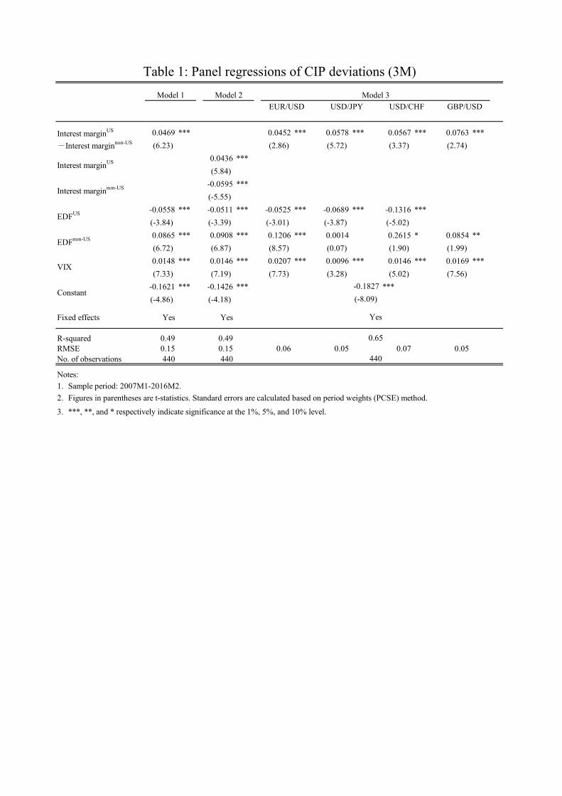
0.0469 *** 0.0452 *** 0.0578 *** 0.0567 *** 0.0763 ***(6.23) (2.86) (5.72) (3.37) (2.74)
0.0436 ***(5.84)
-0.0595 ***(-5.55)
-0.0558 *** -0.0511 *** -0.0525 *** -0.0689 *** -0.1316 ***(-3.84) (-3.39) (-3.01) (-3.87) (-5.02) 0.0865 *** 0.0908 *** 0.1206 *** 0.0014 0.2615 * 0.0854 **(6.72) (6.87) (8.57) (0.07) (1.90) (1.99)0.0148 *** 0.0146 *** 0.0207 *** 0.0096 *** 0.0146 *** 0.0169 ***(7.33) (7.19) (7.73) (3.28) (5.02) (7.56)
-0.1621 *** -0.1426 *** ***(-4.86) (-4.18)
Fixed effects Yes Yes
R-squared 0.49 0.49RMSE 0.15 0.15 0.06 0.05 0.07 0.05No. of observations 440 440
Notes:1. Sample period: 2007M1-2016M2.2.
3. ***, **, and * respectively indicate significance at the 1%, 5%, and 10% level.
Table 1: Panel regressions of CIP deviations (3M)
-0.1827
Interest marginUS
Interest marginnon-US
EDFUS
Model 1
Interest marginUS
-Interest marginnon-US
Model 2 Model 3EUR/USD USD/JPY USD/CHF GBP/USD
Figures in parentheses are t-statistics. Standard errors are calculated based on period weights (PCSE) method.
Constant
EDFnon-US
VIX
Yes
0.65
440
(-8.09)

0.0469 *** 0.0510 *** 0.0736 ***(6.23) (6.54) (8.42)
-0.0558 *** -0.1093 *** -0.1163 ***(-3.84) (-7.60) (-8.62) 0.0865 *** 0.1353 *** 0.1386 ***(6.72) (11.17) (9.78)0.0148 *** 0.0147 *** 0.0158 ***(7.33) (6.06) (5.56)
-0.1621 *** -0.1976 *** -0.2389 ***(-4.86) (-4.93) (-5.07)
Fixed effects Yes Yes Yes
R-squared 0.49 0.50 0.48RMSE 0.15 0.16 0.18No. of observations 440 440 440
Notes:1. Sample period: 2007M1-2016M2.2.
3. ***, **, and * respectively indicate significance at the 1%, 5%, and 10% level.
Figures in parentheses are t-statistics. Standard errors are calculated based on period weights (PCSE) method.
Constant
VIX
Table 2: Panel regressions of CIP deviations of different terms
CIP deviation (6M) CIP deviation (1Y)
Interest marginUS
-Interest marginnon-US
EDFnon-US
EDFUS
CIP deviation (3M)Dependent variable:
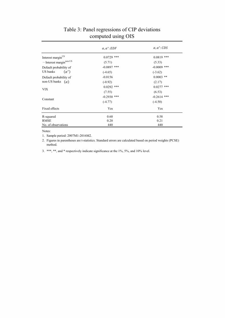
0.0729 *** 0.0819 ***(5.71) (5.33)
-0.0897 *** -0.0009 ***(-4.65) (-3.62) -0.0156 0.0003 **(-0.92) (2.17)0.0292 *** 0.0277 ***(7.55) (6.53)
-0.2930 *** -0.2614 ***(-4.77) (-4.50)
Fixed effects Yes Yes
R-squared 0.60 0.58RMSE 0.20 0.21No. of observations 440 440
Notes:1. Sample period: 2007M1-2016M2.2.
3. ***, **, and * respectively indicate significance at the 1%, 5%, and 10% level.
Table 3: Panel regressions of CIP deviationscomputed using OIS
Interest marginUS
-Interest marginnon-US
Default probability ofUS banks
Default probability ofnon-US banks
VIX
Constant
Figures in parentheses are t-statistics. Standard errors are calculated based on period weights (PCSE)method.
𝛼, 𝛼∗: 𝐸𝐷𝐹 𝛼, 𝛼∗: 𝐶𝐷𝑆
𝛼∗
𝛼

0.0597 ***(6.13)
-0.0572 ***(-5.23) -0.0475 ***(-2.74) -0.0431 ***(-2.84) 0.0926 ***(6.65)0.0307(1.63)0.0135 ***(6.51)
-0.1359 ***(-4.00)
Fixed effects Yes
R-squared 0.50RMSE 0.15No. of observations 440
Notes:1. Sample period: 2007M1-2016M2.2.
3. ***, **, and * respectively indicate significance at the 1%, 5%, and 10% level.
Table 4: Panel regressions of CIP deviation (3M)with the third-country effect
Interest margin3rd country
EDF3rd country
Constant
Interest marginnon-US
Interest marginUS
EDFnon-US
Figures in parentheses are t-statistics. Standard errors are calculated based on period weights(PCSE) method.
EDFUS
VIX

-2.8470 *** -2.8276 *** -3.8069 *** -2.1985 *** -1.6965 ***(-9.36) (-6.15) (-4.05) (-5.45) (-3.03)
-2.5289 ***(-4.34) 3.0476 ***(8.51)
-0.0334 * -0.0332 * 0.0298 -0.0645 *** -0.1369 ***(-1.74) (-1.74) (0.87) (-2.64) (-4.14) 0.0730 *** 0.0733 *** 0.1010 *** 0.0224 0.0933 0.0857 *(5.60) (5.63) (6.82) (1.28) (0.64) (1.68)0.0112 *** 0.0108 *** 0.0126 *** 0.0141 *** 0.0141 *** 0.0120 ***(5.05) (5.51) (3.14) (3.95) (3.91) (4.18)
-0.0469 -0.0460 ***(-1.54) (-1.58)
Fixed effects Yes Yes
R-squared 0.56 0.56RMSE 0.12 0.12 0.05 0.04 0.06 0.04No. of observations 348 348
Notes:1. Sample period: 2008M12-2016M2.2.
3. ***, **, and * respectively indicate significance at the 1%, 5%, and 10% level.
348
Figures in parentheses are t-statistics. Standard errors are calculated based on period weights (PCSE) method.
Table 5: Panel regressions of the impact of monetary policy divergenceon CIP deviation (3M)
VIX
Constant-0.0806(-3.09)
Yes
0.72
BS (monthly growth rate)US
-BS (monthly growth rate)non-US
BS (monthly growth rate)US
BS (monthly growth rate)non-US
EDFUS
EDFnon-US
EUR/USD USD/JPY USD/CHF GBP/USDModel 1 Model 2 Model 3

0.0437 ***(5.61)
-0.0338 ***(-3.68) 0.0313 ***(2.70)0.0028(1.64)
-0.1044 ***(-3.34) 2.5463 ***(7.74)
-3.6760 ***(-12.31)
0.2443 **(2.13)0.6720 ***(8.75)0.3509 ***(5.29)0.7787 **(2.43)
Log likelihood 141.49No. of observations 110
Notes: 1. Sample period: 2007M1-2016M22.
3. ***, **, and * respectively indicate significance at the 1%, 5%, and 10% level.4.
Conditional standard deviation
Dependent variable: CIP deviation
C0
C1
C2
C3
Liquidity shock
Figures in parentheses are z-statistics. Standard errors are calculated based onBollerslev-Wooldridge method.
Liquidity shock is calculated as the residual of the regression of USD LIBOR-OIS spread on US banks’ EDF.
VIX
Constant
Mean equation
Variance equation
Table 6: CIP deviation and market liquidity
Interest marginUS
-Interest marginJP
EDFUS
EDFJP
𝜎𝑡