rehabilitation and maintenance system: state optimal … is an integer nonlinear knapsack problem...
TRANSCRIPT

TECHNICAL REPORT STANDARD TITLE PAGE
1. Report No. 2. Gove>rnment Accession No. 3. Recipient's Catalog No.
f------,--------,----------__j_-----------------4----------------4. Title and Subtitle 5. Report Date
January 1981 6. Performing Organization Code
Rehabilitation and Maintenance System State Optimal Fund Allocation - Program II ( RAMS-SOFA~_-=-'2)~--------------!-------~---:-;------l
8. Pedorming Organization Report No. 7. Authorls)
Don T. Phillips, Chiyyarath V. Shanmugham, Farhad Ghasemi-Tari, Robert L. Lytton
9. Performing Organization Nome and Address
Texas Transportation Institute The Texas A&M University System College Station, Texas 77843
----------------~ 12. Sponsoring Agency Nome and Address
Texas State Department of Highways and Public Transportation; Transportation Planning Division
P. 0. Box 5051 Austin, Texas 78763
15. Supplementary Notes
Research Report 239-2 10. Work Unit No.
1 l. Contract or Grant No.
Research Study 2-18-79-239 13. Type of Report ond Period Covered
. · September, 1978 Interlm - January, 1981
14. Sponsoring Agency Code
Research Study Title: Pavement Rehabilitation Fund A-location 16. Abstract
The Rehabilitation and Maintenance System - State Optimal Fund Allocation Program II (RAMS-SOFA-2) has been developed to aid the Texas State Department of Highways and Public Transportation in determining the optimal statewide strategy and fund allocation district by district. The program is specially designed to make decisions on rehabilitation and maintenance work on Interstate and spine networks on a statewide basis. The program uses a dynamic programming technique. The complete documentation on the program and an example problem are presented in this report. The model developed and the program can be utilized to determine the fund allocation to the residencies of an individual district.
17. Key Words
Pavements, Rehabilitation and Maintenance, Fund Allocation, Dynamic Programming
18. Distribution Statement
No restrictions. This document is available to the public through the National Technical Information Service, Springfield, Virginia 22161
19. Security Classif. (of this report) 20. Security Classif. (of this page) 21. No. of Pages 22. Price
Unclassified Unclassified 141 Form DOT F 1700.7 IB·69l

REHABILITATION AND t1AINTENANCE SYSTEM STATE OPTH1AL FUND ALLOCATION - PROGRAM I I
( RAMS-SOFA-2)
by
Don T. Phi 11 ips
Chiyyarath V. Shanmugham
Farhad Ghasemi-Tari
Robert L. Lytton
Research Report Number 239-2
Pavement Rehabilitation Fund Allocation
Research Project 2-18-79-239
conducted for The Texas State Department of Highways and
Public Transportation
by the
Texas Transportation Institute The Texas A&~1 University System
January 1981

ABSTRACT
The Rehabilitation And Maintenance System - State Optimal Fund
Allocation Program II (RAMS-SOFA-2) has been developed to aid the Texas
State Department of Highways and Public Transportation in determining the
optimal statewide strategy and fund allocation district by district. The
program is specially designed to make decisions on rehabilitation and
maintenance work on Interstate and spine networks on a statewide basis. The
program uses a dynamic programming technique. The complete documentation on
the program and an example problem are presented in this report. The model
developed and the program can be utilized to determine the fund alloca-
tion to the residencies of an individual district.
i

SUMMARY
This report describes the State Optimal Fund Allocation Program 2 of
the RAMS (Rehabilitation And Maintenance System) family of computer programs
developed by the Texas Transportation Institute to aid the Texas State
Department of Highways and Public Transportation to optimally allocate
rehabilitation and maintenance funds between the Districts. The report
contains a detailed description of the mathematical model, an algorithm
to solve the problem, a computer program based on the algorithm, and
a user•s manual.
An overview of all of the RAMS programs and how they are used
sequentially in the fund allocation process is given in the first
report of this series, Research Report 239-1, 11 Rehabilitation and Main
tenance Systems: The Optimization Models ...
The problem that is solved with the program described in this
report is an integer nonlinear knapsack problem with multiple resource
constraints. The algorithm developed uses dynamic programming
methodology. A diverging branch dynamic programming model was developed
for the problem. Each branch of the dynamic programming model is
considered as a District, in which a set of maintenance strategies must
be selected. The objective is to maximize the summation of calculated
utilities subject to the limited resources of materials, equipment
and manpower. The results obtained by solving each branch (District)
are then used for allocation of the state-wide highway maintenance
budget through maintenance Districts. That is, all the branches of the
nonserial dynamic programming model are related to a single state variable.
i i

(amount of the budget), while each branch of a serial dynamic programming
problem with multi-dimensional state variables must be solved.
A computer program has been written based on the developed algorithm
and has been tested on an example problem which has three Districts with 10
highway segments considered for rehabilitation or maintenance in each
District. A user•s guide and program listing is provided in the Appendix.
; ; ;

IMPLEMENTATION STATEMENT
The Texas Transportation Institute at Texas A&M University developed
the Rehabilitation And Maintenance System- State Optimal Fund Allocation -
Program II to help the Texas State Department of Highways and Public
Transporation to determine and distribute optimally the rehabilitation and
maintenance funds among the various districts in the State of Texas. The
RAMS-SOFA-II is to be used in conjunction with the other programs in the
RAMS family of programs. This report is intended as a working document
which can be used by implementation workshops to train Texas SDHPT
personne 1 in the use of RAMS-SOFA-II programs.
DISCLAIMER
The contents of this report reflect the views of the authors who are
responsible for the facts and the accuracy of the data presented herein.
The contents do not necessarily reflect the official views or policies of
the Federal Highway Administration. This report does not constitute a
standard, specification or regulation.
iv

ABSTRACT
SUMMARY
IMPLEMENTATION STATEMENT
LIST OF FIGURES
LIST OF TABLES .
CHAPTER 1 - INTRODUCTION
TABLE OF CONTENTS
CHAPTER 2 - ANALYSIS OF THE HIGHWAY ~1AINTENANCE PROBLEM
CHAPTER 3 - FORMULATION OF THE MATHEMATICAL f10DEL . . .
3.1 -A Dynamic Programming Model for Maintenance Strategic
i
ii
iii
vi
vii
1
5
10
Planning for a Single District . . . . . . . . . . . 10 3.2- A Dynamic Programming Model for r~aintenance Strategic
Planning Considering Multiple Districts 14
CHAPTER 4 - OPTIMIZATION OF THE t10DEL
4.1 -The Imbedded State Approach 4.2 - The Hybrid Algorithm ... 4.3- A t~odified Hybrid Algorithm . . . . . 4.4 - A Multiple District Optimization Example
CHAPTER 5 - SUMMARY
REFERENCES .
APPENDIX A - DEVELOPMENT OF ALGORITHt,1S TO SOLVE THE STATE
22
22 35 53 57
72
73
OPTH1IZATION PROBLEM . . 74
A. 1 - Scope of Hybrid Algorithm . . . . . . . . . . 75 A.2 - The Imbedded State Approach . . . . . . . . . 76 A.3 - Calculation of Initial Lower and Upper Bounds 81 A.4 - Development of the Hybrid Algorithm . . . . . . 86 A.5- Modifications of the Hybrid Algorithm for Large
Scale Nonlinear Knapsack Problem . . . 97
APPENDIX B - DOCUMENTATION OF THE COMPUTER PROGRAM . . . . 101
APPENDIX C - INPUT DATA AND OUTPUT OF THE EXAt~PLE PROBLEM 105
APPENDIX D - LISTING OF C0~1PUTER PROGRA~1 115
v

Figure
1
2
LIST OF FIGURES
Schematic Representation of the Allocation of Funds \~ithin and Between Districts . . . . .
Flow Chart for Hybrid Algorithm .............. .
vi
18
92-96

Table
I
II
III
IV
v VI
VII
VIII
IX
X
XI
XII
XI II
XIV
XV
XVI
c. 1
C.2
LIST OF TABLES
DEDUCT VALUES OF THE DIFFERENT DISTRESSES ON FLEXIBLE PAVEMENT •••.•.••.•••..••
Rj(Xj) -OBJECTIVE FUNCTION COEFFICIENTS •••••••
Aij(Xj) - CONSTRAINT COEFFICIENTS ••••••••••
SOLUTION OF THE SURROGATE PROBLEM AS A FUNCTION OF RHS
HIGHWAY SEGMENT DATA ••••
CURRENT RATINGS OF SEG~1ENTS
GAIN-OF-RATING MATRIX •.
ROAD DETERIORATION FACTORS FOR RAM STRATEGY 1
ROAD DETERIORATION FACTORS FOR RAM STRETEGY 2
ROAD DETERIORATION FACTORS FOR RAM STRATEGY 3
ROAD DETERIORATION FACTORS FOR RAM STRATEGY 4
ROAD DETERIORATION FACTORS FOR RAM STRETEGY 5
ROAD DETERIORATION FACTORS FOR RA~1 STRATEGY 6
RESOURCE REQUIREMENTS ••
OPTIMAL ~1AINTENANCE DECISIONS
OPTIMAL BUDGET UTILIZATION ••
INPUT DATA FOR EXAMPLE PROBLEM • • •
OUTPUT OF EXAMPLE PROBLEM •••
vii
7
24
24
42
60
61
62
63
64
65
66
67
68
69
70
71
106
112

CHAPTER I
INTRODUCTION
The allocation of funds for the rehabilitation and maintenance of
the Texas State highway system required the use of a systematic approach
to maximize return of the taxpayers dollars and to use all available resources
most effectively. Until recently, the establishment of funding levels
allocated to different highway segments have been based upon historical
allocation formulas. Recently, a 0-1 integer linear programming model has
been proposed for allocating the rehabilitation and maintenance funds to
the highway segments in a network which is based upon needs and expected
benefits, considering a one-year period of time (9). However, there is
still a need for an appropriate model to project desirable funding levels
for both single and multiple year rehabilitation and maintenance programs (10).
A second major problem currently being approached is that of distributing the
rehabilitation and maintenance funds among the 25 Districts within the
State of Texas (8).
The strategic objective of the rehabilitation and maintenance of
the Texas highway system is the selection of the optimal policy for each
highway segment in a highway network in order to maximize the total
effectiveness of all maintenance activities scheduled for the entire
highway network in each year of a perpetual sequence of years. This is
an optimization process, requiring a sequence of interrelated decisions
within and between each funding period. Each single period can be con
sidered individually as an optimization problem in which the objective
is to find the most effective maintenance policy, subject to the existing
manpower, equipment, materials, and cost limitations.
1

The single-period optimization is a 11 knapsack type 11 problem with mul
tiple-resource constraints. An earlier attempt to find a solution to
this single-period optimization problem was made by Ahmed (1) who for
mulated the problem as a 0-1 integer linear programming problem. As a
result of this formulation, a large scale 0-1 problem was solved heuristi
cally and a near-optimal solution was obtained.
An alternative approach to the single-period optimization is to for
mulate the problem as a 11 nonlinear knapsack problem11 (NKP) which signi
ficantly reduces the number of variables and eliminates all the constraints
except the resource constraints (8). A promising solution approach to handle
NKP is discrete dynamic programming. Although this approach reduces the
dimensionality of the decision variables, it suffers from the fact that
the existence of more than three resource constraints renders this approach
computationally intractable. This is the well-known problem of dimension
ality of state variables in the dynamic programming technique. One way
to reduce the M-state variable dynamic programming problem to a single
state variable problem is through the use of Lagrangian multipliers (3, 5).
However, the problem of duality gaps, which is likely in the case of
discrete variables, makes this approach somewhat dubious. An alternative
method to reduce the dimensionality of the state variables is by employ-
ing the 11 imbedded state 11 technique (6). Althou.gh the comparative efficiency
of both the Lagrangian and imbedded state approach is a questionable
matter, and probably depends on the structure of the problem, the latter
approach is reported to be relatively more effd:jent for NKP ~
A fundamental advantage in using dynamic programming techniques for single
period optimization is that it provides a bookkeeping record of returns for
2

different maintenance funding levels which can be used for the overall
distribution of funds, in an optimal manner, throughout different years
in a given District. Development of a dynamic programming based model
also provides the capability of distributing funds over all Districts in
the State for a given budget cycle (8). Conversely, by using 0-1 integer
programming for single-period optimization, the overall distribution of
funding levels would be either impossible or a very difficult and time
consuming task.
This report presents a model which is capable of distributing
available rehabiliation and maintenance funds over a single period
throughout all Districts in the State, and allocating other available
resources within each District. The resulting model is also capable of
optimally distributing limited funds through a finite time horizon for
a single District or to allocate funds available in a single time period
to different residencies within the District. When it is used for time
staging of projects, it is called RAMS-DT0-2 (District Time Optimization
No. 2) and when it is used to optimally allocate funds between residencies
for a single time period it is called RAMS-D0-2 (District Optimization,
No. 2). A user's manual on RAMS-DT0-2 with changes in the program and
the input data and results of an example problem will be presented in
a forthcoming report.
When the same program is used to allocate funds available in a
single time period between Districts, it is called RAMS-SOFA-2. (State
Optimal Fund Allocation Progra111 No. C7 An over•tie~~ of the RAt4S (Rehabilitation
and Maintenance System) family of programs that have been developed by
the Texas Transportation Institute to aid the Texas State Department of
Highways and Public Transportation to optimally allocate rehabilitation
3

and maintenance funds between and within the Districts is given in the
first report of this series, Research Report 239-1, "Rehabilitation and
Maintenance Systems: The Optimization Models." A new dynamic programming
algorithm, capable of efficiently handling multiple constraints, will
also be discussed.
4

CHAPTER 2
ANALYSIS OF THE HIGH!~AY t1AINTENANCE PROBLEM
Allocation of funds for highway maintenance operations is one of the
basic components of the general rehabilitation and maintenance management
system. In general, the basic components of a maintenance management
system include maintenance standards, inventories of maintenance equipment,
maintenance work loads, management information systems, and capital budgeting.
The last component, capital budgeting, will likely become more stringently
controlled in the future, and hence there exists a need for systematic,
optimal allocation of these limited resources. Moreover, the use of an
analytical technique for systematic allocation of available resources at
the District level can identify maintenance practices that can potentially
save money through more efficient utilization. Before describing the
mathematical development of the problem, some useful terms should be
defined:
a. Highway segment. A highway segment is a portion of a highway
section or a combination of highway sections under consideration.
This term is used to identify several highway sections which are
similar or identical in traffic condition and environmental
factors which affect the effectiveness of maintenance and reha
bilitation activities.
b. Analysis period. The analysis period is a time duration greater
than the expected life of any maintenance or rehabilitation
method.
c. Types of distress. The usual categories of distress types for
flexible pavements are: (1) rutting, (2) raveling, (3) flushing,
5

(4) corrugation, (5) roughness, (6) alligator cracking, (7) longi
tudingal cracking, (8) transverse cracking, and (9) patching.
d. Maintenance Strategy. A maintenance strategy is an activity
selected for a highway segment in order to increase the pavement
rating above a specified minimum requirement. Numerous strategies
can be applied to each pavement segment. Among the more generally
used strategies are the following: (l) strip seal, (2) fog seal,
(3) seal coat, (4) light patching, (5) extensive patching and
seal coating, (6) seal coat and planned thin overlay, (7) plant-mix
seal or open~graded friction course, (8) thin overlay (less than
two inches of asphalt concrete), (9) moderate overlay (two to
three inches of asphalt concrete), (10) heavy overlay (three to
six inches of asphalt concrete), and (11) reconstruction.
e. Pavement condition. The following criteria are used for deter
mining current pavement condition: (1) the current pavement con
dition rating of each segment for each type of distress, (2) the
potential gains of rating of each segment for each maintenance
strategy and type of distress, (3) the pavement survival rate for
each type of distress through a given time period for each type
of pavement, (4) the minimum rating requirement of each segment
for each type of distress over a specified time period.
f. Current pavement condition rating. The present condition of the
pavement is determined by evaluation of the highway segment
with respect to various types of distress. The rating score is
obtained by subtracting the total "deduct values" associated
with various types of distress from 100. Table 1 represents an
example of deduct values for six types of distress for flexible
pavement ( 2).
6
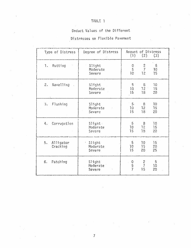
TABLE 1
Deduct Values of the Different
Distresses on Flexible Pavement
Type of Distress Degree of Distress Amount of Distress (l) (2) (3)
1. Rutting Slight I 0 2 5 Model~ate 5 7 10 Severe 10 12 15
2. Rave 11 i ng Slight I 5 8 10 I Moderate 10 12 15 I I I Severe 15 18 20 I
') Flushing Slight 5 8 10 I .j.
Moderate 10 12 15 Severe 15 18 20
I i
4. Corrugation Slight 5 8 10 I ~~ode rate 10 12 15 l
I Severe 15 18 20 I
,... Alligator Slight 5 10 15 o. Cracking Moderate 10 15 20
Severe 15 20 25
6. Patching Slight 0 2 5 ~lode rate 5 7 10 Severe 7 15 20
7

g. Potential gain in rating. Potential gain in rating is defined
as the net expected increase in pavement rating for each segment
for each type of distress and maintenance strategy.
h. Pavement survival rate. When a maintenance strategy is applied
to a highway segment, the pavement condition must achieve a high
enough rating to survive for one year. Therefore, the survival
probability immediately following a maintenance activity is one.
As time passes, the pavement deteriorates and the survival probabil
ity of that segment is reduced.
i. Maintenance activity. Maintenance activity is a general term
for the varous types of work that can be done to increase the
rating score of a given pavement section.
j. Minimum rating requirement. The ninimum rating requirement is
used as an indication of when a maintenance activity must be
scheduled. There are two such indicators: the first indicator
results when the distress rating for any single type of distress
falls below a minimum acceptable rating; the second indicator
occurs when the total of all distress type ratings are less than
the minimum total rating requirement.
k. Resource information. The restrictions on the availability of
the resources usually appear as a set of constraints on the
mathematical model. For strategic planning of pavement main
tenance and rehabilitation, the resources are categorized in the
following groups: (1) material and supply, (2) equipment,
(3) personnel' and (4) cristrict budget.
8
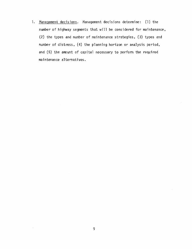
1. Management decisions. Management decisions determine: (1) the
number of highway segments that will be considered for maintenance,
(2) the types and number of maintenance strategies, (3) types and
number of distress, (4) the planning horizon or analysis period,
and (5) the amount of capital necessary to perform the required
maintenance alternatives.
9

CHAPTER 3
FORMULATION OF THE MATHEMATICAL MODEL
The zero-one integer linear program formulation described by Phillips
and Lytton (9) for optimal allocation of resources within a district is the
basic model for pavement maintenance strategy planning. A detailed descrip
tion of this model and a solution process is given in Ahmed (1) and Ahmed
et al. (2). For a realistic problem, the model will involve a large number
of zero-one decision variables and a very large number of constraints. For
example, consider a District highway network with 200 highway segments, with
ten maintenance alternatives per segment. Assume that there are 15 resource
constraints and 5 different types of distress. Hith a planning horizon
of 10 years as the period of analysis, the model will have approximately
2000 decision variables, 200 multiple choice constraints, 16 resource
constraints including budget, 10,000 minimum rating constraints and
2,000 minimum overall rating constraints.
For the state-wide system optimization, a zero-one integer linear
programming model whould be approximately 20 times larger.
3.1 A Dynamic Programming Model for Maintenance Strategic Planning for a Single District
An alternative approach, which will alleviate the diffi-
culties identified in the previous section, is the development of a
dynamic programming model for problem solution. Both the problem of
allocating resources within a District and the problem of allocation of
total budget between Districts can be handled by such a model. The
decomposition of dynamic programming converts the larger problem into a
sequence of smaller problems through which the process of achieving an
10

optimal solution to the overall problem becomes easier. Further, the
capability of obtaining the optimal solution values as a function of
resource availability provides an inherent sensitivity analysis that
can take into account the different budget levels at each District. As
described in a subsequent section, the optimization process can be
performed only once in each District, and the required information for
distributin9 the budget to the.different Districts can be achieved
by solving a single dynamic programming problem.
This dynamic programming model for allocation of resources at the
District level can be represented as a nonlinear knapsack problem. In
general, a nonlinear knapsack model can be presented in this form shown
bel ow.
Prob 1 em A:
~1ax. f(~) = N 2::
j=l
Subject to:
N 2::
j=l a .. (X.) < b. lJ -J - 1
r. (X.) J -J
xj is contained in sj.
i=l,2, ... ,M
j = 1, 2, ... N
Problem A is a general form of the resource allocation problem.
In the specific case of the highway maintenance allocation problem N
is the number of high1t1ay segments in a district; Kj is the number of dif
ferent types of maintenance strategies that can be applied to highway
11

segment j; bi is the available amount of resource type i; Xj is a decision
variable taking values 1, 2, ... , Kj which indicates what strategy is being
selected; aij is the amount of resource type i consumed by highway segment
j if strategy Xj is being selected; rj (Xj) is the return benefit obtained
from using maintenance strategy Xj on highway segment j, and M is the total
number of limited resources.
The form of the mode 1 presented as Problem A can be expanded by
defining its individual terms as follows:
Problem B
Max.
Subject to:
N z:
j=l
N z:
j=l
N z:
j=l
N z:
j=l
N N z:
j=l r. (X.) = z: L1 J. J J j=l
S . (X.) L l . L2. < TS g 9J J J J -
Ef.(X.) L1. L2. < TEf J J J J -
H .(X.) L1. L2. < TH qJ J J J - q
C . ( X . ) L l . L2 . < T C J J J J -
[N0 ~ ]
L2 . z: z: D.k(X.) P.kt(X.) J k=l t=l J J J J
g = 1, 2, ••• , NG
f = 1, 2, ••. , NF
q = 1, 2, ... ,No
where the terms of the model are defined as follows:
( 3. 1)
(3.2)
(3.3)
(3.4)
(3.5)
Cj =the overhead cost function of strategy Xj at highway segment j.
12

Efj =consumption of equipment type fat highway segment j.
Hqj = consumption of work force type q as a function of strategy
Xj at highway segment j.
Llj =the length of highway segment j.
L2j =the width of highway segment j.
N = the member of highway segments.
N0 = the number of distress types.
NF = the number of different types of equipment.
NG =the number of different types of material.
NQ = the number of different types of workforce.
NT = the number of years in the analysis period.
Pjkt = pavement survival probability as a funtion of strategy Xj
for the type of distress kat period t, in highway segment j.
Sgj = consumption of type g material per unit surface area as a
function of strategy Xj at highway segment j.
TC = total budget available, in dollars.
TEf =total amount of type f equipment available (equipment-day).
THq =total amount of q work force (human resource) available
(person-day).
TSg = total amount of type g material available.
In order to compare the dimensionality of the 0-1 integer linear
program and dynamic programming, consider the example used earlier. It
was stated that the zero-one integer linear program formulated for the
problem involves approximately 2000 decision variables and 12,216 constraints.
The nonlinear knapsack model for the same problem involves only 200 decision
variables and only 16 inequality constraints. This illustrates a significant
13

reduction of 1800 decision variables and 12,200 inequality constraints.
It must be recognized that the decision variables in the later model take
on 10 different values. However, the use of a proper solution technique,
dynamic programming, will yield an efficient solution to the problem.
3.2 A Dynamic Programming Model for Maintenance Strategic Planning Considering Multiple-Districts
The models discussed in Section 3.1 have been developed to allocate
funds within a specific District. In this section, the problem of state
wide fund allocation will be discussed. In particular, a model will be
developed to allocate the state-wide budget to the Districts and at the
same time, to allocate resources within individual Districts. The task
of projecting the required budget levels for the annual maintenance program
is also considered in this model.
Consider the nonlinear knapsack model discussed as Problem A. This
formulation is a general representation of the allocation of resources
within a highway District. The availability of each resource, such as
equipment, materials, and manpower is determined by the District engineer
and usually has fixed values. However, the amount of funds available to
the Texas State Department of Highways and Public Transportation is
determined by the State legislature. Recently, a systematic method for
allocating the statewide budget to Districts has been proposed by Phillips
and Lytton (8). The proposed method provides a range of budget allocations
to each District. An optimal maintenance policy is determined for the
selected number of possible budget levels within each District. The
overall maintenance policy at this state level is then determined through
an overall synthesis and optimization model based upon dynamic programming.
14

In order to be certain that the Interstate and other spine networks are
maintained at acceptable levels of service in all Districts, a more desirable
approach to the problem of allocating the statewide spine network budget to
individual Districts is to develop a model capable of handling both the within
and between District allocation process at the same time. The mathematical
representation of such a model in the form of a nonlinear knapsack problem is
presented below.
Problem C
D N Max. L: L:
d=1 j=1 r.d(X.)
J J
Subject to:
where
N L: a .. d(X.) < b.d i = 1 ' 2, . ' M-1
j=1 lJ J - 1
d = 1 ' 2, . . . D '
D N L: L: c.d(x.) < TC
d=l j=l J J
x. is contained in sjd d = 1 ' 2' . D J '
j = 1, 2, . N ' sjd = ( l ' 2, . . . Kjd) '
aijd = the amount of resource type i (excluding overhead cost)
consumed as a function of strategy Xj' for highway segment j at
District d.
bid= total amount of type i available resource (excluding budget level)
at District d.
15

Cjd = the amount of consumption costs which is a function of the
strategy Xj' for highway segment j in District d.
D = the number of Districts in the analysis.
Kjd = the number of maintenance strategies that can be applied to
highway segment j in District d.
M = the number of resource constraints excluding costs.
rjd =the return function of strategy Xj' for highway segment
j, in District d.
TC = total amount of available budget for entire state.
x. = the decision variable indicating the type of strategy to be J
selected.
Problem C can be decomposed into two separate problems. The first is a
decomposition of the problem according to Districts. Each District can then
be considered as a single state in a statewide dynamic programming formulation.
The second problem is a decomposition of all District subproblems into indi-
vidual highway segments which yields a problem similar to Problem A. This
process can be illustrated by expanding Problem C.
Problem D
N Max. z
j=l
N N
16

Subject to:
N I a .. 1(x.)
1 J J j=l
N I
j=l a .. 2(x.) lJ J
fo r i = 1 , 2 , • • • , M- 1
N N I c.1(x.) + I c. 2(x.) +
j=l J J j=l J J
N I
j=l
N I
j=l
c.D(x.) J J
a .. D( X.) lJ J
< b., - _,
< b.2 - _,
< b.D - _,
< TC
Referring to Problem D, the limitations on all the resources are considered
independently for each District with the exception of the limitation on the budget
level (TC) which interrelates the decisions in all Districts. However, the
allocation process within each District could be developed independently if
it were developed as a function of budget level in that District. That is, a
vector presenting the optimal return as a function of budget level in each
District could be obtained. These District benefits and associated cost levels
could be used for the allocation of the total budget to individual Districts.
17

I-' 00
OIST. 1
OIST. 2
r11 r21 j, t ~·· "1
z, ;.. z21 . \ z31
r -=:4 Se. g. I ---~.' s:. g., __ ,.,... · :. , 1 1 _ -, 2 _ .
yll i y21 y31
000
000
! r. 1
J '
z. 1 : z. 1 1 J, r--"---~ J+ ' ~ I--- , I S~g. [ ooo -~ J :~ 000
y . 1 1 __j y. +1 1 J ' J '
l ~ !
z12~, L.... z22~·· ' z32 ~zj 2 ' zj+l 2 ----;,;;...o_; Seg. -. --"~ Seg. ·-·--~ ooo ·-·' S~g. ~----.. ~ ooo . 1 -- '' 2 -- 000 .. J ! ~ 000
..... ,;>1' ..... ., ....... ..... ~ .......
yl2 d y22 d 1 y32 Yj,2 d 1 yj+1 12 22 j,2
r N, 1
zN,l rJ,z~l ,-·--ol S eg ·I / -1 N IV y N '1 1 N+ 1 '1
4 zN,2 ~ ZN+l ,l -~[ S~g·1=-: - A -YN,2 d i YN+l;2
N,2 r-; .
c ( j ' ~ s li<
0 0
z OIST. t t, 1 ...
000
000
0
DIST. 0
-y t '1 0 0
0 0
r r ' t 1,0 A 2,0 \ z \ z z I 1~0 · .. ·• I 2,0 I 3,0
Seg. 1 ~ Seg. ~ 1 . ' 2 •
y . y ~ y 1,0 , 2,0 3,0
!
d1, 0 d2 ,0
r. t
~!J'
z z.+ ooo -----. J ~,tooo
; . 000 . .. 000
- I J ~-
y j , t . i y N+ 1 , t j,t
r. 0 J '
z. 0 L z. +l D ZN D
~J, ' J ' '
000 ~ 000 ..
000 ~ 000 - -Yj,O ; yj+l,O YN,D
d. J,O
Figure 1. Schematic Representation of the Allocation of
Funds Within and Between Districts
0
0
0
dN,O

This two-level allocation process can be suitably performed using a non
serial dynamic programming model. This model is illustrated schematically in
Figure 1. In this figure, each branch represents the allocation of resources
within a District, and the node S from which each branch diverges represents
the allocation of the total budget to each individual District.
In each branch there will be N stages representing the number of segments
in that branch {Districts), and D branches diverging from NodeS. Each branch
may be solved as an initial-value problem in terms of Zjt' This is accomplished
using forward recursion carrying Zjt as an extra state variable. At the final
stage the return vector, which is a function of the state variables, will be
obtained for each branch. The state variables represent the consumption of the
resources such as types of equipment, materials, personnel, and the total budget
level. Among these state variables, only the consumption of the budget is the
subject of further optimization and all other state variable inputs are fixed.
As a result, the returns in each District, as a function of budget level, are
obtained. Considering each District as a single stage in the dynamic program
ming model, a decision must be made with regard to the allocation of budget
levels to each District in order to obtain the maximum return.
Referring to Figure 1, it can be seen that each branch involves a multiple
constraint dynamic programming problem. These constraints are divided into two
groups. The first group is represented by a state vector yjd' The second
group, rehabilitation cost, is represented by a single~state variable, Zjd'
This separation has just been justified; i.e., the cost constraint interrelates
the decision-making process between the different branches, which enables the
group of constraints represented by yit to be considered independently within
each branch.
Consider District d; allocation of resources to this District using a
19

dynamic programming technique results in the following recursive equations: ~
Rdl (Zld' v1d) = ~1ax. r1d(Xj)
over
fqr a fixed d
~
Rdj(ZJd' Yjd) =Max. rjd(Zj) +Max. Rj-l,d(Zj=l,t'yj-l,d)
for j = 2 , 3 , ••• , N
over ~
o < A.d(x.) < v1.d - J J -
for j = 2, 3, ... , N
The state recursion equations are:
j = 2, 3, •.• , N
~ ~
yj-l,t = yjt- Ajt(Xj) j = 2, 3, .•• , N
where the state variables are defined as
and
Zjt =the amount of budget available for stages (segments) j,
j+l, ... ,N. ~
Yjt = the vector whose components represent the amount of each
type of resource available for stages (segments) j, j + 1, ... , N.
20

The recursive equations developed for District t can be applied
to all Districts, i.e., d = l, 2, ... ,D. After a dynamic programming
solution procedure is applied to each District, the return RNd (ZNd, YNd)
will be obtained. Since the first group of constraints is not involved in
the allocation of budget to Districts, let Rd (Zd) = RNd (ZNd' YNd}. The
distribution of budget levels to each District is then obtained by solving
the following problem:
Problem E:
D Max. E
d=l
Subject to:
11here
D E
d=l
S~ = the vector of the budget levels in the final stage of branch
d ((District d).
R~ = the return vector obtained in the final stage of branch d
(District d) .
Problem E is a one-dimensional (single linking constraint) nonlinear
knapsack model which can also be solved with dynamic programming techniques.
The optimal solution resulting from solving Problem E will define the
optimal budget level, Z~*, and after obtaining this value, the optimal
set of maintenance policies for every segment of each District can be
recovered. 21

CHAPTER 4
OPTIMIZATION OF THE t~ODEL
This chapter presents the development of the required algorithm
for solving separable nonlinear, multi-dimensional knapsack problems.
The algorithm is called a 11 hybrid algorithm 11, and it is essentially a
dynamic programmming approach in the sense that the problem is divided
into smaller subproblems. However, the idea of fathoming the partial
solution by branch and bound is incorporated within the algorithm.
The main feature of the hybrid algorithm is its capability of reducing
the state-space which otherwise would present an obstacle in solving
multiple-constraint dynamic programming problems. Part of this reduction
is due to the use of the imbedded-state approach, which reduces an M
dimensional dynamic program to a one-dimensional problem. Other reductions
are made through fathoming the state-space and subsequent elimination
of state-space regions, which tend to eliminate inferior solutions when
compared to the predetermined lower bound or updated lower bound.
The use of a surrogate constraint methodology is implemented in the
algorithm to obtain initial lower and upper bounds for the objective
function. At each stage, the lower and upper bounds are also updated
by use of a surrogated problem, and the updated upper bound is used
for termination criteria. The procedure for updating lower and upper
bounds in the surrogated problem is very efficient. In addition, the
primary advantages of using the surrogate problem to estimate these
bounds, are (1) it provides a narrow range between the lower and upper
bound, and (2) it might provide the optimal solution to the problem at
the first step.
22

A modification of the hybrid algorithm has been developed for appli-
cation to large scale NKP's. However, the modified algorithm, though
computationally much faster, may not provide an optimal solution to some
problems, but rather will obtain a near-optimal solution. The modified
algorithm follows roughly the same procedure as the hybrid algorithm.
However, instead of evaluating all promising solution spaces, it attempts
only to improve the lower bound calculated by the surrogated problem.
The details of the hybrid and the modified hybrid algorithm are
presented in Appendix A. The documentation and the user's guide to the
computer programs are given in Appendices B and C. The algorithms will
now be explained by use of a simple example.
4.1: The Imbedded State Approach
Consider a District highway network problem, with 4 highway segments.
There are 5 maintenance strategies available per segment. The two con
straints deal with the budget and one type of resource. Therefore=
N = 4
K· = 5 J
M = 2
Considering the model presented in Problem A, X. is contained ins. i.e. J J
x. E: s. = (1, 2, 3, 4, 5) J J
forj = 1, 2, 3, 4.
The objective function coefficients and the constraints are given in
Table II and Table III respectively. The right hand sides (availability
of resources) are 28 in each constraint.
23

j
*
i
1
2
1
2
l
2
1
2
*
TABLE II
Rj(Xj) -OBJECTIVE FUNCTION COEFFICIENTS
X. J
E: s. J
j 1 2 3 4
1 0 2 3 5
2 0 3 4 5
3 0 6 9 11
4 0 4 7 10
j is the index on the highway segments.
j 1
l 0
l 0
2 0
2 0
3 0
3 0
4 0
4 0
TABLE I II
A .. (X.) - CONSTRAINT COEFFICIENT 1J J
x. J
E: s. J
2 3 4
6 8 9
3 4 5
7 10 12
4 6 8
8 10 12
6 8 9
5 6 9
/!. () 12 <.)
i = the index on the constraints. j = the index on the highway segments.
24
5
8
6
13
11
5
11
7
14
10
15
12
10
5

Solution:
Stage 1 Calculations
j = 1 ' K = K = 5 1
The imbedded-state space for stage 1 is
G1 = {co,o), (6,3), (8,4), (9,5), (11,7)}
F1 - G - 1
r 1 = ( 0, 2 , 3, 5, 8)
The T 1 and TS,, matrices are created using elements of F1 and r 1.
Ts1
Row xl Pointer gl rl ~ to
Stage 0
1 1 -- 0 0 0
2 2 -- 6 3 2
3 3 -- 8 4 3
4 4 -- 9 5 5
5 5 -- 11 7 8
Since each element of F1 satifies the feasibility conditions,
{0,0) < (28, 28)'
( 6 ,3) < (28, 28),
{8,4) < (28, 28)'
(9,5) < (28, 28),
(11,7) < (28, 28)'
25

none of these solutions are eliminated and hence
and
The updated version of TS1,and T1 will be the same as the ones before
since no points are eliminated.
Stage 2 Calculations
J = 2, K = K2 = 5
~ = {<o.o) {7,4), {10,6}, (12,8), {14,1o)}
in F e 1
The number of elements in F2 is the product ofK2 and the elements
F2 = { {0,0), {6,3), {8,4), {9,5), {11,7), {7,4), {13,7) (15,8),
(16,9), 18,11), (10,6), (16,9), (18,11), (10,6), (16,9),)
(18,11), (10,6), (16,9) (18,10), (19,11), (21,13), (12,8),
(18,11), (20,12), (21,13), 23,15), (14,10), (20,13), (22,12),
{23,15), (25,17)}.
The T2 and TS2 matrices are generated as follows.
26
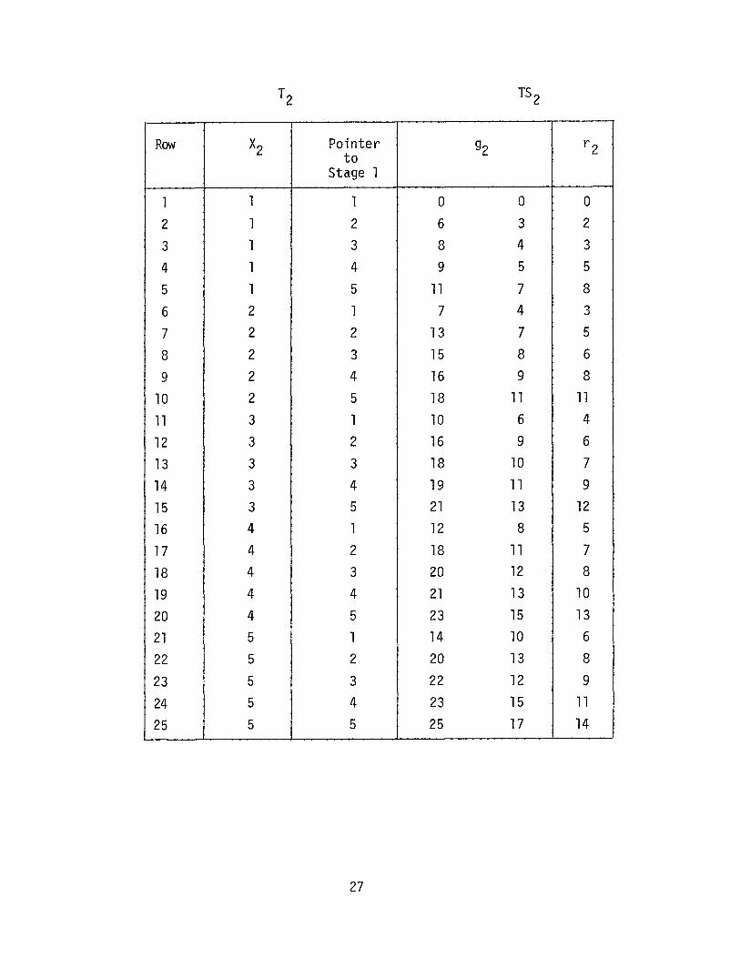
Row x2 Pointer g2 r2 to
Stage 1
1 1 1 0 0 0
2 1 2 6 3 2
3 1 3 8 4 3
4 1 4 9 5 5
5 1 5 11 7 8
6 2 1 7 4 3
7 2 2 13 7 5
8 2 3 15 8 6
9 2 4 16 9 8
10 2 5 18 11 11
11 3 1 10 6 4
12 3 2 16 9 6
13 3 3 18 10 7
14 3 4 19 11 9
15 3 5 21 13 12
16 4 1 12 8 5
17 4 2 18 11 7
18 4 3 20 12 8
19 4 4 21 13 10
20 4 5 23 15 13
21 5 1 14 10 6
22 5 2 20 13 8
23 5 3 22 12 9
24 5 4 23 15 11
25 5 5 25 17 14
27
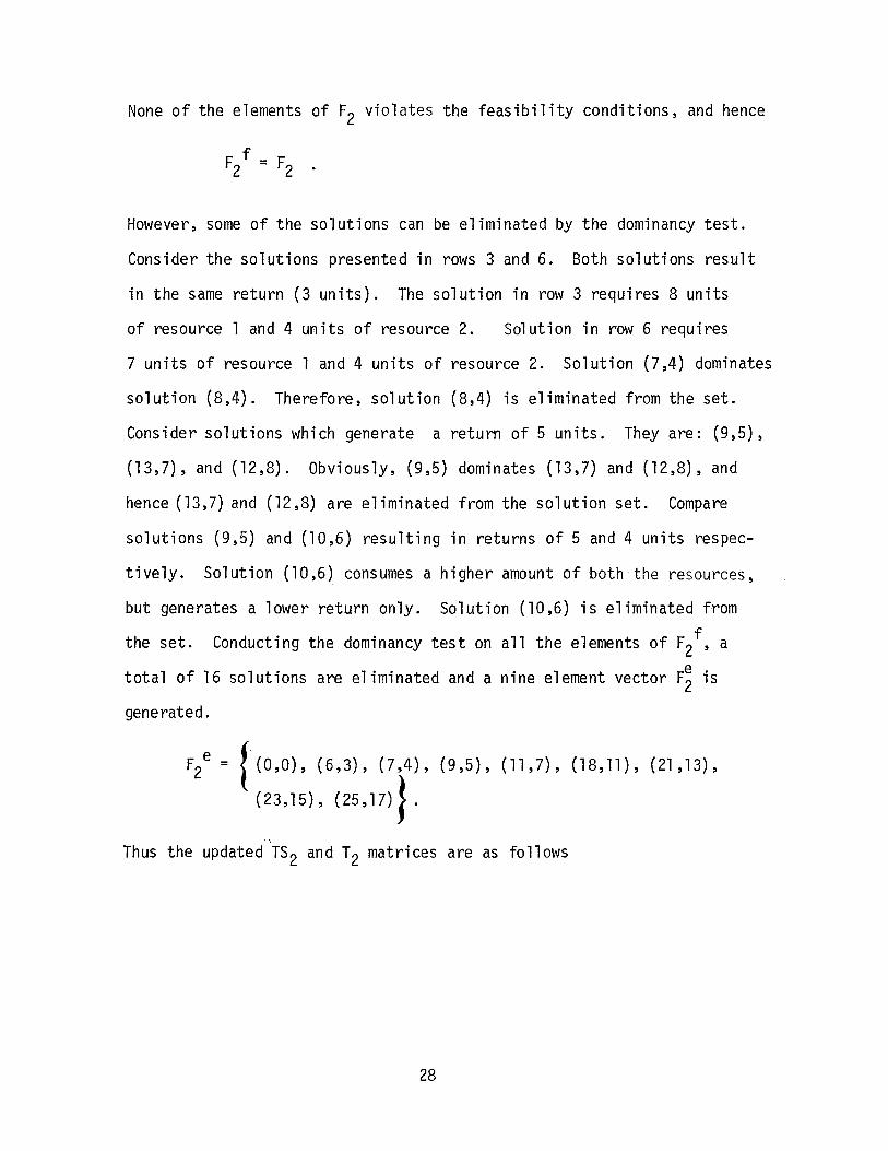
None of the elements of F2 violates the feasibility conditions, and hence
However, some of the solutions can be eliminated by the dominancy test.
Consider the solutions presented in rows 3 and 6. Both solutions result
in the same return (3 units). The solution in row 3 requires 8 units
of resource 1 and 4 units of resource 2. Smution in row 6 requires
7 units of resource 1 and 4 units of resource 2. Solution (7,4) dominates
solution (8,4). Therefore, solution (8,4) is eliminated from the set.
Consider solutions which generate a return of 5 units. They are: (9,5),
(13,7), and (12,8). Obviously, (9,5) dominates (13,7) and (12,8), and
hence (13,7) and (12,8) are eliminated from the solution set. Compare
solutions (9,5) and (10,6) resulting in returns of 5 and 4 units respec
tively. Solution (10,6) consumes a higher amount of both the resources,
but generates a lower return only. Solution (10,6) is eliminated from
the set. Conducting the dominancy test on all the elements of F2f, a
total of 16 solutions are eliminated and a nine element vector F~ is
generated.
F e 2 = { (0,0), {6,3), (7,4), {9,5), {11,7), (18,11), (21,13),
(23, 15)' {25, 17)}.
Thus the updated 'Ts2 and T2 matrices are as follows
28

l Row x2 Pointer 92 r2
to Stage l
l l l 0 0 0
2 l 2 6 3 2
3 2 l 7 4 3
4 l 4 9 5 5
5 l 5 11 7 8
6 2 5 18 11 11
7 3 5 21 13 12
8 4 5 23 15 13
9 5 5 25 17 14
Stage 3 Calculations
J = 3, K = K3 = 5
G3 = {(0,0), (8,6), (10,8), (12,9), (15,12)}
and
e Since G3 and F2 have 5 and 9 elements respectively, F3 will have 45
elements. The elements of F3 with the associated returns are listed in
the TS 3 matrix.
29

Row x3 Pointer to
93 r3
Stage 2
1 1 1 0 0 0
2 1 2 6 3 2
3 1 3 7 4 3
4 1 4 9 5 5
5 1 5 11 7 8
6 1 6 18 11 11
7 1 7 21 13 12
8 1 8 23 15 13
9 1 9 25 17 14
10 2 1 8 6 6
11 2 2 14 9 8
12 2 3 15 10 9
13 2 4 17 11 11
. . . . . .
. . . . . .
. . . . . 33 4 6 30 20 22
34 4 7 33 22 23
35 4 8 35 24 24
36 4 9 37 26 25
37 5 1 15 12 13
38 5 2 21 15 15
39 5 3 22 16 16
40 5 4 24 17 18
41 5 5 26 19 21
42 5 6 33 23 24
43 5 7 36 25 25
44 5 8 38 27 26
45 5 9 40 29 27 I
30
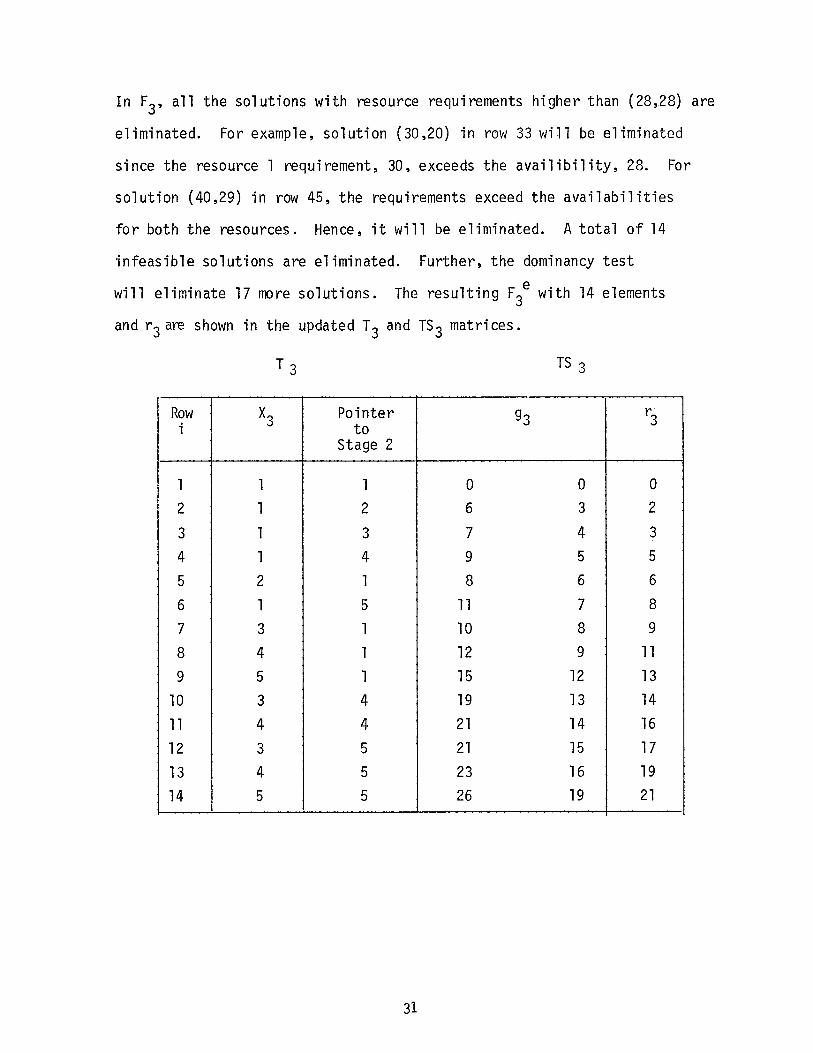
In F3, all the solutions with resource requirements higher than (28,28) are
eliminated. For example, solution (30,20) in rovJ 33 will be eliminated
since the resource 1 requirement, 30, exceeds the availibility, 28. For
solution (40,29) in row 45, the requirements exceed the availabilities
for both the resources. Hence, it will be eliminated. A total of 14
infeasible solutions are eliminated. Further, the dominancy test
will eliminate 17 more solutions. The resulting F3e with 14 elements
and r3 are shown in the updated T 3 and rs3 matrices.
TS 3
Row x3 Pointer g3 r3 i to
Stage 2
1 1 1 0 0 0 2 1 2 6 3 2
3 1 3 7 4 3
4 1 4 9 5 5
5 2 1 8 6 6
6 1 5 11 7 8
7 3 1 10 8 9
8 4 1 12 9 11
9 5 1 15 12 13 10 3 4 19 13 14
11 4 4 21 14 16
12 3 5 21 15 17
13 4 5 23 16 19
14 5 5 26 19 21
31

Stage 4 Calculations
J = 4, K = K4 = 5
G4 = {(0,0), (5,4), (6,8), (9,12), (10,15)}
~d
F4 = G4o F3 ~ contains 70 elements of which 37 elements are eli
minated by feasibility and dominancy tests. The resulting F4e will have
33 solutions and are shown in the following r4 and rs4 matrices.
32

Row x4 Points 94 Y'3 i to
Stage 3
1 1 1 0 0 0
2 1 2 6 3 2
3 2 1 5 4 4
4 1 4 9 5 5
5 1 5 8 6 6
6 3 1 6 8 7
7 2 3 12 6 7
8 1 6 11 7 8
9 1 7 10 8 9
10 4 1 9 12 10
11 5 1 10 15 11
12 1 8 12 9 11
13 2 6 10 11 12
14 1 9 15 12 13
15 3 5 14 14 13
16 1 10 19 13 14
17 2 8 17 13 15
18 1 11 21 14 16
19 2 7 16 16 16
20 1 12 21 15 17
21 2 9 20 16 17
22 3 8 18 17 18
23 1 13 23 16 19
33
Row x4 Pointer g4 r4 i to
Step 3
24 4 7 19 20 19
25 3 9 21 18 20
26 5 7 20 23 20
27 1 14 26 19 21
28 4 8 21 21 21
29 5 8 22 24 22
30 2 13 28 20 23
31 3 11 27 22 23
32 4 9 24 24 23
33 3 12 27 23 24
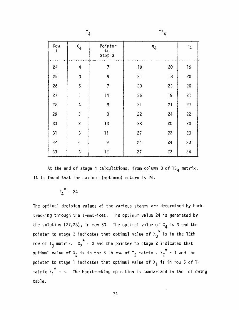
At the end of stage 4 calculations, from column 3 of TS 4 matrix,
it is found that the maximum (optimum) return is 24.
* R4 = 24
The optimal decision values at the various stages are determined by back
tracking through the T-matrices. The optimum value 24 is generated by
the solution (27,23), in row 33. The optimal value of x4 is 3 and the
* pointer to stage 3 indicates that optimal value of x3 is in the 12th
* row of T3 matrix. x3 = 3 and the pointer to stage 2 indicates that
* optimal value of x2 is in the 5 th row of T2 matrix . x2 = 1 and the
pointer to stage 1 indicates that optimal value of x1 is in row 5 of T1 * matrix x1 = 5. The backtracking operation is summarized in the following
table.
34

* Stage x. Pointed to A1
. ( X . ) A2
. ( X • ) r. (X.) j J Stage j-1 J J J J J J
4 3 12 6 8 7
3 3 5 10 8 9
2 1 5 0 0 0
1 5 - 11 7 8
* g4 = (27,23) R = 24 4
4.2 The Hybrid Algorithm
The solution of the same example problem will now be obtained using
the hybrid algorithm. The algorithm requires an initial lower and upper
bounds to the objective which is obtained by the surrogate constraint
methode 1 ogy.
The surrogate problem of Problem A is as follows:
Problem E
N t1ax I
j=l
subject to
N M I I
j=l i=l
r. J
(X.) J
M a. A .. (Xj) 2. I a. b.
1 1J i=l l 1
n I a. = 1
1 i=l
a.>O,i=l,2, ... ,~1 1
35

j=l,2, ... ,N
Let
~1 A.(X.) = I a. A .. (X.) J J i=l 1 lJ J
M and B = I a; b;
i =1
where
[I] defines the largest integer value less than or equal to I.
Then, the surrogate problem is:
max N I A.(X.) < B
j=l J J -
j = l, 2, ... , N.
For the example problem Aj and rj are as follows:
j A.(X.) J J
1 (0, 4, 6, 7, 9)
2 ( 0, 5, 8, 10, 12)
3 ( 0, 7, 9, 10, 13)
4 ( 0' 4, 7, 10, 12)
36
r. (X.) J J
(0, 2, 3, 5, 8)
(0, 2, 4, 5, 6)
( 0, 6, 9, 11, 13)
(0, 4, 7, 10, 11) I

The solution to the surrogate problem is obtained using the dynamic pro
gramming techniques in tabular form (7).
Stage 1 Calculations
Table of Returns for Stage 1
xl 1 2 3 4 5 * * Al 0 4 6 7 9 Rl xl
rl 0 2 3 5 8 B
0-3 0 - - - - 0 1
4-5 0 2 - - - 2 2
6 0 2 3 - - 3 3
7-8 0 2 3 5 - 5 4
9-28 0 2 3 5 8 8 5
37

Stage 2 Calculations
x2 1
B ~ 0
r2 0
0 - 3 0
4 2
5 2
6 3
7 5
8 5
9 8
10 8
11 6
12 - 13 8
14 8
15 8
16 8
17 :8
18 8
19 - 20 18
21 - 28 8
Table of Cumulative Returns for Stages 2 and 1
2 3 4
5 8 10
3 4 5
- - -- - -3 - -
3 - -
3 - -
3 4 -
5 4 -
5 4 5
6 4 5
8 6 5
11 7 7
11 9 7
11 9 8
11 12 10
11 12 10
11 12 13
11 12 13
38
5
12 R * 2 X * 2 6
- 0 1
- 2 1
- 3 2
- 3 1,2
- 5 1
- 5 1
- 8 1
- 8 1
- 8 1
6 8 1 ,2
6 11 2
6 11 2
8 11 2
8 12 3
9 12 3
11 13 4
11 13 4

Stage 3 Calculations Table of Cumulative Returns for Stages 3, 2, 1
x3 1 2 3 4 5
B A3 0 7 9 10 13 R * 3 ~*
r3 0 6 9 11 13
0 - 3 0 - - - - 0 1
4 2 - - - - 2 1
5 3 - - - - 3 1
6 3 - - - - 3 1
7 5 6 - - - 6 2
8 5 6 - - - 6 2
9 8 6 9 - - 9 3
10 8 6 9 11 - 11 4
11 8 8 9 11 - 11 4
12 8 9 9 11 - 11 4
13 8 9 11 11 13 13 5
14 11 11 12 13 13 13 4,5
15 11 11 12 14 13 14 4
16 11 14 14 14 13 14 2,3,4
17 12 14 14 16 15 16 4
18 12 14 17 16 16 17 3
19 13 14 17 19 16 19 4
20 13 14 17 19 18 19 4
21 13 17 17 19 18 19 4
22 13 17 17 19 21 21 5
23 13 17 20 19 21 21 5
24 13 18 20 22 21 22 4
25 13 18 20 22 21 22 4
26 13 19 21 22 21 22 4
27 13 19 21 23 24 24 5
28 13 19 21 23 24 24 5
39

Stage 4 Calculations
Table of Cumulative Returns for Stages 4, 3, 2, and 1
x4 1 2 3 4 5
A4 0 4 7 10 12 R * X * B
4 4 r4 0 4 7 10 11
0 - 3 0 - - - - 0 1
4 2 4 - - - 4 2
5 3 4 - - - 4 2
6 3 4 - - - 4 2
7 6 4 7 - - 7 3
8 6 4 7 - - 7 3
9 9 7 7 - - 9 1
10 11 7 7 10 - 11 1
11 11 10 9 10 - 11 1
12 11 10 10 10 11 11 1 ,5
13 13 13 10 10 11 13 1,2
14 13 15 13 12 11 15 2
15 14 15 13 13 11 15 2
16 14 15 16 13 13 16 3
17 16 17 18 16 14 18 3
18 17 17 18 16 14 18 3
19 19 18 18 19 17 19 1 ,4
20 19 18 20 21 17 21 4
21 19 20 20 21 20 21 4
22 21 21 21 21 22 22 5
23 21 23 21 23 22 23 2,4
24 22 23 23 23 22 23 2,3,4
25 22 23 24 24 24 24 3,4,5
26 22 25 26 24 24 26 3
27 24 25 26 26 25 26 3,4
28 24 26 26 27 25 27 4
40

The maximum value of the returns is 27 when B equals 28. The corresponding
optimal decisions for the various stages are obtained by tracing back
through the stage calculations and are illustrated below:
Stage B X.* A. r.* j J J J
4 28 4 10 10
3 18 3 9 9
2 9 l 0 0
l 9 5 9 8
= {5, l' 3, 4)
Similarly, the optimal decisions for various values of B can be determined
by tracing back through the stage calculations. The solution of the surro
gate problem for various values of B are shown in Table IV. In Table IV,
the solution forB equal to 27 is eliminated since B = 26 and B = 27
generate the same objective function value, Rsp (27) = Rsp (26) = 26.
In addition, it should be noted that certain values of B generate
alternate optimum solutions; e.g. when B = 25, there are three alternate
optimal decisions.
The initial lower and upper bounds to be used in the hybrid
algorithm are determined as follows:
UB0 = Rsp (28) = 27.
41

TABLE IV. SOLUTION OF THE SURROGATE PROBLEM
AS A FUNCTION OF RIGHT HAND SIDE
State (B) Return R(B) . Optimal decisions
0 0 1 1 1 1
4 4 1 1 2
7 7 1 1 l 3
9 9 1 3 l
10 11 1 1 4 1
13 13 1 1 5 1
13 13 l 1 3 2
14 15 1 1 4 2
16 16 1 1 3 3
17 18 1 1 4 3
19 19 5 1 4
19 19 l 1 3 4
20 21 1 1 4 4
22 22 1 1 4 5
23 23 5 1 4 2
25 24 5 1 3 3
25 24 1 1 5 5
25 24 1 2 4 4
26 26 5 1 4 3
28 27 5 3 4
42
X

The lower bound LB0
is the largest optimal return value of the surrogate
problem with the corresponding optimal decisions being feasible to the
original problem.
Consider B = 28; * X = (5,1,3,4)
Since
= 11 + 0 + 10 + 9 = 30 > 28 = b1,
the first constraint is violated and x* = (5,1,3,4) is an infeasible
solution.
Let B = 26; x* = (5,1,4,3)
= 11 + 0 + 12 + 6 = 29 > 28 = b1
implies that x* = (5,1,4,3) is also infeasible.
Consider B = 25; * X = (1,2,4,4)
= 0 + 7 + 12 + 9 = 28 = b1,
x* satisfies first constraint.
= 0 + 4 + 9 + 12 = 25 < 28 = b1
* implies second constraint also is satisfied. X = (1,2,4,4) is a feasible
solution to the original problem.
Therefore
LB0 = Rsp (25) = 24.
43

Solution of the Example Problem:
Let i
Stage 1 Calculations
Gl = (0, 0), (6,3), (8,4), (9,5), (11,7)
R1 = (0, 2, 3, 5, 8)
No points are eliminated by the feasibility and dominancy tests. The T1 and TS1 matrices are as follows.
Row xl Pointer 9\ Rl(gil) - to
Stage 0
1 1 -- 0 0 0
2 2 -- 6 3 2
3 3 -- 8 4 3
4 4 -- 9 5 5
5 5 -- 11 7 8
= 1 gil = (0,0)
4 UBl1l = R1 (gll) + l rt (kt)
t=2
= 0 + (6 + 13 + 11) = 30
44
UB211 = R1 (g11) + Rsp (B - B1(g11) )
= 0 + R (28 - O + O ) sp 2
= 0 + Rsp (28)
= 0 + 27 = 27
g11 = (0,0) is not discarded.
Let i = 2 g12 = (6,3)
4 (g12) + l rt (kt)
t=2
= 2 + (6 + 13 + 11)
= 32
= 2 + Rsp (24)
= 2 + 23 = 25
g12 = (6,3) is not eliminated.
45

Let i = 3
UB2 3 3 R (28 - 8 ; 4) 1 = + sp
= 3 + R (22) = 3 + 22 sp
= 25 > LB0
•
913 = (8,4) is not discarded.
Let i = 4 4 91 = (9,5)
= 5 + 21 = 26 > LB . 0
914 = (9,5) is not eliminated.
Let i = 5 5 91 = (11 ,7)
UB2 5 8 R (28 - 11 ~ 7) 1 = + sp
=8+R (19) sp
= 8 + 19 = 27 > LB • 0
915 = (11,7) is not eliminated.
T1 and TS1 matrices are as shown before.
46

The upper and lower bounds are updated as follows:
UB1 = Min { M1n { UB21 i } , UB 0 J = Min { Mjn f 27,25,25,26 ,27 J ' 27} = Min {25,27} = 25.
LB1 = Max {M~x ~ R(gli)l, LBo}
= Max { M~x ( 0,2,3,5,81, 24}
= Max { 8,24}
= 24.
Stage 2 Calculations
First, T2 and TS2 matrices are generated similar to the imbedded
state approach. T2 and TS2 are given below:
Row x2 Points to i R2(g2i) g2 i stage 1 1 1 1 0 0 0
2 1 2 6 3 2 3 2 1 7 4 3 4 1 4 9 5 5 5 1 5 11 7 8 6 2 5 18 11 11 7 3 5 21 13 12 8 4 5 23 15 13 9 5 5 25 17 14
47

The following can be easily observed.
UB1 21 = 0 + 24 = 24{ LB 1
UB221 = 0 + Rsp(28) = 27 { LB1
g21 = (0,0) is not eliminated.
Simi 1 arly,
g25
= (11 ,7), and g26 = (18,11) are not to be eliminated.
Let i = 7 g2 7 = (21,13)
UB1 27 = 12 + 24 f LB1
UB2 7 12 R (28-21;13) 2 = + sp
=12+R (11). sp
= 12 + 11 = 23 < LB1.
g27 = (21,13) is eliminated.
Similarly g28 = (23,15) and g2
9 = (25,17) are also eliminated. The
updated T2 and TS2 matrices are as follows.
48

Row x2 Pointer to g2 i i stage 1
1 1 1 0 0
2 1 2 6 3
3 2 1 7 4
4 1 4 9 5
5 1 5 11 7
6 2 5 18 ll
The bounds are updated as follows:
UB2 =Min {Min {27,25,26,26,27,26), 25}
= Min { 25 ,25l = 25.
LB2 = Max { Max { 0,2 ,3 ,5 ,8, 11), 24}
=Max {11,24} = 24.
LB2 :f UB2•
Stage 3 Calculations
R2(g2i)
0
2
3
5
8
11
After eliminating the solutions which are infeasible and are
dominated, T3 and rs3 matrices are obtained as follows:
49

Row x3 i
1
2 3 4 5 6 7 8 9
10 11
12 13 14
Let i = 1
UB1 1 = 0 + 11 = 3
1
1 1 1 2 1 3 4 5 3 4 3 4 5
Pointer to stage 2
1
2 3 4 1 5 1 1 l
4 4 5 5 5
i R3(g3i) 93
0 0 0
6 3 2
7 4 3 9 5 5
8 6 6
11 7 8 10 8 9 12 9 11
15 12 13 19 13 14
21 14 16
21 15 17
23 16 19 26 19 21
S. "1 1 2 3 1m1 ar y g3 , g3 ,
4 5 6 7 8 93 , 93 , 93 , 93 , and 93 are eliminated. ·
For i = 9 -14 the computations are as fo 11 ows:
i i UB1 i UB2 i 93 3 3
9 15 12 24 28
10 19 13 25 25
11 21 14 27 27
12 21 15 28 28
13 23 16 29 28
14 26 19 32 25
50

UB1 3i and UB23i, fori = 9,14, are not less than LB2. Therefore
g3i (i = 9,14) are not eliminated. The updated T3 and TS 3 matrices are
as follows:
Row x3 Pointer to g i i stage 2 3
1 5 1 15 12 2 3 4 19 13 3 4 4 21 14 4 3 5 21 15 5 4 5 23 16 6 5 5 26 19
The bounds are updated as follows:
UB 3 ~ Min { Min ~28,25 ,27 ,28 ,28,251, 25}
~Min {25,25 }~ 25.
LB3 ~Max {Max \l3,14,16,17,19,2ll, 24}
~ Max { 21 ,24} ~ 24.
Stage 4 Calculations
i R3(g3 )
13 14 16 17 19 21
After eliminating the solutions which are infeasible and dominated,
the T4 and TS4 matrices are generated as follows:
51

Row x4 Pointer to g4 i R4(g4i) i stage 3
1 1 1 15 12 13
2 1 2 19 13 14
3 1 3 21 14 16
4 1 4 21 15 17
5 2 1 20 16 17
6 1 5 23 16 19
7 3 1 21 18 20
8 1 14 26 19 21
9 2 5 28 20 23
10 3 3 27 22 23
11 4 1 24 24 23
12 3 4 27 23 24
Since UB1 4i (i = 1 ,11) are less than 24 = LB 3, g4i (i = 1,11) are
eliminated from the set. The updated T4 and TS4 matrices are as
follows:
Row x4 i
1 3
Pointer to stage 3
4
UB2 l = 24 4
UB4 = Min { 24,25 } = 24
LB4 = Max { 24,24} = 24.
LB4 = UB4.
*
g4 i R4(g4i)
27 23 24
The optimal solution is found with R = 24. The optimal decision variable
52

are determined by tracing back through the T-matrices.
* X = (5,1,3,3).
4.3: A Modified Hydrid Algorithm
The example problem will again be solved using the modified hybrid
algorithm. After calculation of lower and upper bounds, three points with
the objective function value of 24 are obtained, as shown in Table III. I
Any of these points can be considered as X , i e.
Case 1: X' = (5, 1 ' 3, 3) or
Case 2: VI = ( 1 ' 1 ' 5, 5) or 1\
Case 3: x• = ( 1 ' 2, 4, 4)
In this example we consider the first two cases individually to
demonstrate the performance of the modified algorithm:
Case 1:
xl = (5, 1 ' 3, 3) ; Rsp (Xl) = 24
x2 = (5, 1 ' 3' 4); Rsp (X2) = 27
Stage 1
1 1 x1 > x2 =>s1 = { xll} = {s }. Tl TS1
Row xl Pointer to i Rl ( gl i ) i stage 0 gl
1 5 - 11 7 8
53

Stage 2
x1 2
> x/ ~> s2 = { x/} = { 1 }
Row x2 Pointer to g i R2(g2i) i stage 1 2
1 1 1 11 7 8
Stage 3
xl 3? x2 3=> s3 = { xl 3 J = { 3}
T3
Row x3 Pointer to g3 i R3(g3i) i stage 2
1 3 1 21 15 17
Stage 4
xl 4 < x4=>S4 = { xl 4, xl 4 + 1, . • . , x2 4}
= { 3,4}
Row x4 Pointer to i R4(g4i) i stage 3 g4
1 3 1 27 23 24 2 4 1 30 27 27
Feasibility test will eliminate g42.
Thus optimal objective function value,
* * R(X) = 24 and X = (5, 1, 3, 3).
54

Case 2:
xl = ( 1 ' 1 ' 5, 5) ' Rsp (Xl) = 24
x2 = ( 5' 1 ' 3' 4) ' Rsp (X2) = 27 -
Stage 1
x, 1 < x, 2
> s, = { 1 ' 2' 3' 4' 5 }
rs1
Row x, Pointer to g i Rl ( gl i) i stage 0 1
1 1 - 0 0 0
2 2 - 6 3 2 3 3 - 8 4 3
4 4 - 9 5 5 5 5 - 11 7 8
None of g1 i is eliminated by the tests.
Stage 2
Row x2 i
1 1 2 1 3 1 4 1 5 1
Pointer to 92 i stage 1
1 0
2 6
3 8
4 9
5 11
UB2 = 25 'I 24 = LB2 55
R2{g2i)
0 0
3 2 4 3
5 5 17 8

Stage 3
Row x4 Pointer to 94i R3(g3i) i stage 2
1 5 1 15 12 13 2 5 2 21 15 15
3 5 3 23 16 16
4 5 4 24 17 18
5 5 5 26 29 21
g35 is eliminated (infeasibility).
Stage 4
Row x4 Pointer to g i R4(g4i) i stage 3 4
1 5 1 25 27 24 2 5 2 31 30 26 3 5 3 33 31 27 4 5 4 34 32 29
2 3 4 Infeasibility eliminates g4 , g4 and g4 . Therefore the
optimal solution is
x*=(l,l,5,5), with R(x*)=24.
5'3

4.4: A Multiple District Optimization Example
The State of Texas is divided into 25 highway Districts. In each
District there are more than 200 highway segments which are considered
annually for rehabilitation and maintenance activities. In each budget
cycle it is necessary to observe or estimate each highway•s pavement condi
tion and also to estimate the condition of the segment in succeeding years.
If any segment does not satisfy the minimum serviceability or maximum
distress requirements, a maintenance strategy should only be considered if its
use results in this segment exceeding the minimum requirements. The
model requires the following data information.
1. A description of the highway segments used in each district.
2. Pavement condition ratings for each segment.
3. The gain-of-rating matrices.
4. The pavement survivor matrices.
5. Resource information in each district.
6. Available state budget.
Since most of the data needed are not readily available at present
for most of the Districts in the state of Texas, a hypothetical example
problem was generated.
The example problem has 3 highway Districts, each with 10 highway
segments to be considered for maintenance in each district. A total
of six maintenance strategies are adopted. They are: (1) seal coat,
(2) 1.0 11 overlay, (3) 2.0 11 overlay, (4) 3.0 11 overlay, (5) 5.0 11 overlay,
and (6) 7.0 11 overlay. Six types of pavement distress are used to
measure the segment deterioration. They are: (1) rutting, (2) alligator
cracking, (3) longitudinal cracking, (4) transverse cracking, (5) failures
per mile, and (6) the serviceability index. The manpower resources are:
57

(1) asphalt cement, (2) grader, (3) loader, (4) truck, (5) grader
operator, (6) loader operator and (7) truck operator. The budget is the
last resource to be considered here.
In each District, highway segments are divided into 2 classes. The
first class consists of 1 U.S. • and 'State highways' and the second type
consists of 'Farm-to-Market' highways.
Highway Segment Information. The following information is needed for
each highway segment within all Districts; (a) Highway type, (b) length
(miles) and (c) width (feet) of each highway segment. The traffic index
and environmental factors are assumed to be unity for this example.
The data required is as shown in Table V.
The current rating of highway segments by distress types are shown
in Table VI. This information is needed for each District.
The enhancement in pavement quality level attained through the
application of a maintenance strategy for various distress types are
shown in Table VII. The quality level cannot be greater than the maximum
possible rating. If an application of any one strategy causes this to
occur, the highway rating is fixed at this maximum level.
Pavement survivor matrices are developed for each distress type
and maintenance strategy combination. All highway segments within each
District are assumed to have identical pavement deterioration curves.
Road deterioration curve fractions for each type of maintenance strategy
are listed in Tables IX, X, XI, XII, and XIII by distress type. The
road deterioration curves are determined by multiplying the road deterior
ation fractions by the maximum quality levels.
The resources constraints need two major inputs: requirements and
availability. The first indicates how much of a given resource will be
58

used by maintenance strategy (per mile-ft. of the pavement) and the second
indicates how much of the resources are available. These are shown in
Table XIV.
The optimum solution to the three District example is given in
Tables XV, and XVI.
Table XV shows the resulting optimal maintenance strategy schedule
for each highway segment in the three Districts. The optimal budget
utilization is shown in Table XVI. As a result of solving each branch
(District) of the dynamic programming model, the minimum required and
the maximum needed funds for a District to maintain the pavement quality
are obtained. Columns 2 and 3 of the Table XVI, indicate the maximum
and minimum budget levels. The sum of maximum budget levels for the
three Districts is 256,000 dollars; but the available budget for the three
Districts is only 250,000 dollars. (If the sum of minimum required
budgets exceeds the available budget, an infeasible solution will result).
The optimum budget levels for the three Districts are shown in Column 4
and the corresponding utilities are shown in Column 5.
59
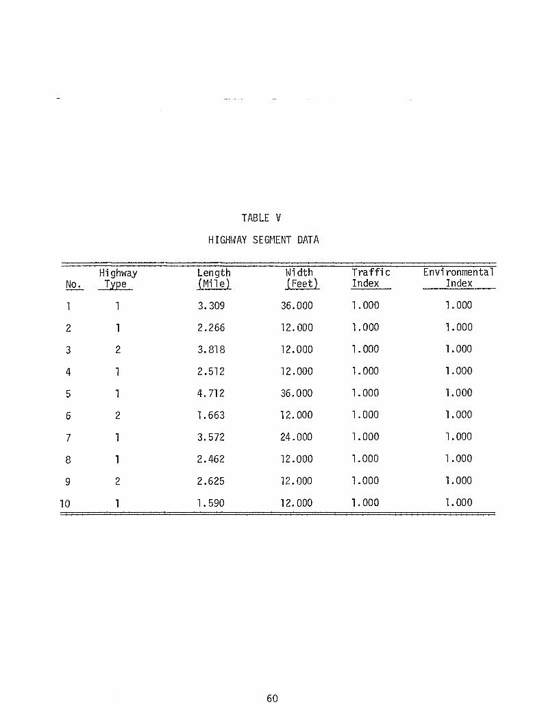
TABLE V
HIGHWAY SEGMENT DATA
Highway Length \!Ji dth Traffic Environmental No. Type (Mi 1 e) (Feet) Index Index
1 1 3.309 36.000 1. 000 1. 000
2 1 2.266 12.000 1. 000 1. 000
3 2 3.818 12.000 1. 000 1. 000
4 1 2.512 12.000 1. 000 1.000
5 1 4.712 36.000 1. 000 1.000
6 2 1.663 12. 000 1. 000 1.000
7 1 3. 572 24.000 1. 000 1. 000
8 1 2.462 12.000 1.000 1. 000
9 2 2.625 12.000 1.000 1. 000
10 1 1. 590 12.000 1. 000 1. 000
60

TABLE VI
CURRENT RATING OF SEGMENTS
Segment DISTRESS T Y P E No. 1 2 3 4 5 6
1 15.000 25.000 20.000 25.000 30.000 40.000
2 5.000 20.000 20.000 25.000 30.000 0.000
3 15.000 10.000 5.000 25.000 30.000 10.000
4 5.000 25.000 25.000 25.000 30.000 40.000
5 5.000 10.000 15.000 5.000 30.000 0.000
6 15.000 25.000 15.000 25.000 30.000 40.000
7 15.000 25.000 25.000 25.000 30.000 40.000
8 15.000 20.000 20.000 25.000 30.000 40.000
9 5.000 25.000 20.000 5.000 30.000 10.00
10 5. 000 5.000 5.000 5.000 30.000 10.000
61

TABLE VII
GAIN-OF-RATING MATRIX
Strategy DISTRESS T Y P E No. 1 2 3 4 5 6
1 0.000 15.000 15.000 15.000 10.000 2.000
2 13.000 19.000 19.000 19.000 24.000 45.000
3 13.000 20.000 20.000 20.000 25.000 45.000
4 15.000 25.000 25.000 20.000 30.000 50.000
5 15.000 25.000 25.000 20.000 35.000 50.000
6 15.000 25.000 25.000 20.000 40.000 50.000
62

TABLE VIII
-PA-VEr1Hff-I}E-fE-RI8PJ\"FI-0N-FAH8RS-FOR-R-&~1-S-FAA"F-E-GV-l
Year DISTRESS T Y P E
1 2 3 4 5 6
1 1. 000 1. 000 1.000 1. 000 1.000 1.000
2 0.930 0.940 0.930 0.920 1. 000 0.900
3 0.910 0.890 0.880 0.860 0.910 0.700
4 0.880 0.890 0.870 0.850 0.780 0.500
5 0.780 0.650 0.670 0.670 0.470 0.400
6 0.310 o. 280 0.370 0.380 0.220 0. 300
7 0.220 0.240 0.320 0.330 0.200 0.200
8 0.150 o. 150 0.180 0.180 0.100 0.100
9 0.070 0.090 0.090 0.090 0.040 0.100
10 0.050 0.070 0.070 0.060 0.010 0.000
11 0.020 0.020 0.020 0.010 0.000 0.000
12 0.020 0.010 0.010 0.010 o.ooo o.ooo 13 0.020 0.010 0.010 0.010 o.ooo o.ooo 14 0.020 0.010 0.010 0.000 0.000 0.000
15 0.010 0.000 0.000 o.ooo o.ooo 0.000
16 o. 010 o.ooo o.ooo o.ooo o.ooo 0.000
17 o. 010 0.000 0.000 0.000 0.000 0.000
18 0.010 o.ooo 0.000 0.000 0.000 0.000
19 0.010 o.ooo 0.000 0.000 0.000 0.000
20 0.010 0.000 0.000 0.000 0.000 0.000
63

TABLE IX
P-AVE MENT-DETERIURATTO~r-FATTORs--FoR-R&l\1-s TRATEGY 2
Year DISTRESS T Y P E
1 2 3 4 5 6
1 1. 000 1.000 l. 000 1.000 1.000 1. 000
2 1. 000 1.000 1. 000 1.000 1. 000 1. 000
3 1.000 0.890 1. 000 1.000 1. 000 1. 000
4 1. 000 0.820 1. 000 1. 000 1. 000- 0.900
5 0.880 0.730 1. 000 1.000 1.000 0.800
6 0.780 0.670 0.750 0.830 1. 000 0.700
7 0.460 0.670 0.500 0.670 1.000 0.600
8 0.250 0.670 0.500 0.670 0.330 0.500
9 0.250 0.670 0.250 0.330 0.330 0.400
10 0.250 0.360 0.000 0.000 0.330 0.300
11 0.000 o. 110 0.000 0.000 0.000 0.000
12 0.000 0.090 0.000 0.000 0.000 0.000
13 0.000 0.000 0.000 0.000 0.000 0.000
14 0.000 o. 000 0.000 0.000 0.000 0.000
15 0.000 0.000 0.000 0.000 0.000 0.000
16 0.000 0.000 0.000 0.000 0.000 0.000
17 0.000 0.000 0.000 0.000 0.000 0.000
18 0.000 0.000 0.000 0.000 0.000 0.000
19 0.000 0.000 0.000 0.000 0.000 0.000
20 0.000 0.000 0.000 0.000 0.000 0.000
64

TABLE X
FAVEMENT-DETERIUR7\TTON--FATTURS_FO_R-R&M -sTRATFGY -3
Year DISTRESS T Y P E
1 2 3 4 5 6
1 1. 000 1.000 1. 000 1.000 1.000 1.,000
2 1.000 1.000 1.000 1.000 1.000 1. 000
3 1. 000 0.950 0.930 0.940 1. 000 1. 000
4 1. 000 0.910 0. 930 0.940 0.890 0.900
5 0.790 0.900 0.400 0.430 0.530 0. 800
6 o. 750 0.610 0.140 o. 180 0.230 0.700
7 0. 750 0.560 0.140 o. 180 0.160 0.600
8 0.750 0.550 0. 120 0.140 o. 150 0.500
9 0.750 0.510 0.070 0.060 0.130 0.400
10 0. 750 0.280 0.020 0.010 0.080 0.300
11 0.330 o. 170 0.000 0.000 0.020 0.000
12 0.250 0.140 0.000 0.000 0.000 0.000
13 0.250 0.140 0.000 0.000 0.000 0.000
14 0.170 0.140 0.000 0.000 0.000 0.000
15 0.080 0.080 0.000 0.000 0.000 0.000
16 0.000 0.010 0.000 0.000 0.000 0.000
17 0.000 0.000 0.000 0.000 0.000 0.000
18 0.000 0.000 0.000 0.000 0.000 0.000
19 0.000 0.000 0.000 0.000 0.000 0.000
20 0.000 0.000 0.000 0.000 0.000 OJOOO
65

TABLE XI
PAVE~1ENf-DE-fERIO RAT-ION·· FAeT0RS- F0R---R-&t1-S-fRA1EGY 4
Year DISTRESS T Y P E
1 2 3 4 5 6
1 1.000 1. 000 1. 000 1. 000 1.000 1. 000
2 1.000 1. 000 1.000 1. 000 1. 000 1. 000
3 1. 000 1. 000 1. 000 1. 000 1. 000 1. 000
4 1. 000 1.000 1.000 1.000 1.000 1. 000
5 1. 000 0. 770 1.000 1. 000 0. 770 0.900
6 0.830 0.640 0.330 0.630 0.510 0.800
7 0.710 0. 580 0.110 0.260 0.480 0.700
8 0.660 0. 530 0.000 0.220 0.360 0.600
9 0.620 0.510 0.000 0. 110 0.330 0.500
10 0.380 0.380 0.000 0.040 0.240 0.500
11 0.300 0.210 0.000 0.000 0.170 0.000
12 0.300 0.190 0.000 0.000 o. 170 0.000
13 0.300 o. 190 0.000 0.000 0.170 0.000
14 0.280 0.170 0.000 0.000 o. 170 0.000
15 0.220 0.150 0.000 0.000 0.170 0.000
16 0.170 0.100 0.000 0.000 o. 170 0.000
17 0.120 0.070 0.000 0.000 0.070 0.000
18 0.040 0.060 0.000 0.000 0.000 0.000
19 0.040 0.060 0.000 0.000 0.000 0.000
20 0.040 0.030 0.000 0.000 0.000 0.000
66

TABLE XI I
. PAVEMENrDETERIORATION-FA-CTDRS-FOR--R&WSTRATEGY 5
Year D I STRESS T Y P E
1 2 3 4 5 6
1 1. 000 1. 000 1. 000 1.000 1. 000 1. 000
2 1. 000 1. 000 1.000 1.000 1. 000 1.000
3 1.000 1. 000 1. 000 1. 000 1. 000 1. 000
4 1. 000 1.000 1. 000 1. 000 1. 000 1.000
5 1.000 1. 000 1.000 1. 000 1. 000 1. 000
6 1 .000 0.710 0.330 0.330 0.750 0.900
7 1.000 0.620 0. 330 0.330 0.590 0.900
8 1. 000 0.440 0.280 0.280 0.500 0.800
9 1. 000 0.290 o. 170 0.170 0.480 0.700
10 1. 000 0.290 0.170 0.170 0.250 0.600
11 0.670 0.290 0.170 o. 170 0.250 0.000
12 0.670 0.170 0.170 0.170 0.250 0.000
13 0. 670 0.140 0.170 o. 170 0.250 0.000
14 0.670 0.140 o. 170 o. 170 0.250 0.000
15 0.220 0.120 o. 170 0.170 0.200 0.000
16 0.000 0.000 0.170 0.170 0.000 0.000
17 0.000 0.000 o. 170 0.170 0.000 0.000
18 0.000 0.000 o. 170 0.170 0.000 0.000
19 0.000 0.000 0.170 o. 170 0.000 0.000
20 0.000 0.000 o. 170 o. 170 0.000 0.000
67

TABLE XIII
PAVD1ENT DETERIORATION-F.II.CTORS FOv-R7JJSTRAlTGY 6
Year DISTRESS T Y P E
1 2 3 4 5 6
1 1. 000 1.000 1.000 1. 000 1. 000 1.000
2 1. 000 1. 000 1. 000 1.000 1. 000 1.000
3 1. 000 1. 000 1.000 1. 000 1. 000 1. 000
4 1. 000 1. 000 1. 000 1. 000 1. 000 0.900
5 1. 000 1. 000 1. 000 1. 000 1. 000 o. 800
6 0. 720 0.490 1. 000 1. 000 0.470 0.700
7 0.670 0.360 1. 000 1. 000 0.360 0.600
8 0.580 0.360 1.000 1. 000 0.320 0.500
9 0.500 0.360 0.650 0.650 0.270 0.400
10 0.500 0.290 0.600 0.600 o. 270 0. 300
11 0.360 0. 270 0.600 0. 600 0.270 0.000
12 0.330 o. 270 0.600 0.600 0.200 0.000
13 0.330 0.270 o. 530 0.510 o. 180 0.000
14 0.280 0.270 0.400 0.400 0.180 0.000
15 0.170 0.210 o. 380 0.380 0.150 0.000
16 o. 170 o. 190 0.210 0.200 0.090 0.000
17 0.170 0.190 0.200 0.000 0.090 0.000
18 o. 170 0.180 0.200 o.ooo 0.090 0.000
19 o. 170 0.110 0.200 0.000 0.090 0.000
20 o. 170 0.090 0.200 0.000 0.090 0. 000
68
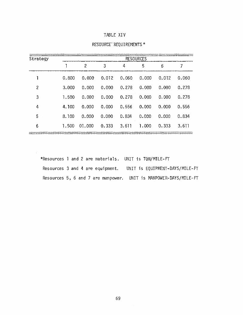
TABLE XIV
RESOURCE-. REQUIRH1ENTS-*
Strategy RESOURCES
1 2 3 4 5 6 7
1 0.800 0.000 0.012 0.060 0.000 0.012 0.060
2 3.000 0.000 0.000 0.278 0.000 0.000 0.278
3 1. 500 0.000 0.000 0.278 0.000 0.000 0.278
4 4.100 0.000 0.000 0.556 0.000 0.000 0.556
5 8.100 0.000 0.000 0. 834 0.000 0.000 0.834
6 1. 500 01.000 0.333 3. 611 1. 000 0.333 3. 611
*Resources 1 and 2 are materials. UNIT is TON/MILE-FT
Resources 3 and 4 are equipment. UNIT is EQUIPMENT-DAYS/MILE-FT
Resources 5, 6 and 7 are manpower. UNIT is MANPOWER-DAYS/MILE-FT
69

TABLE XV
OPTIMAL ~~AINTENANCE DECISIONS
S E G M E N T S
DISTRICT 1 2 3 4 5 6 7 8 9 10
1 5 4 2 2 6 4 4 2 1 1
2 5 5 2 2 2 5 2 2 1 1
3 5 4 2 3 2 6 4 4 1 1
70

TABLE XVI
OPTIMAL BUDGET UTILIZATION
District Budget Uti1 ity Maximum Mininum Optimum
1 71 ,000 66,000 71,000 2171
2 84,000 68,000 78,000 1772
3 101,000 92,000 101,000 1742
TOTAL 250,000 5685
71

CHAPTER 5
~~MMARY
The major purpose of this report was to describe a technique which can be
used in determining the optimal allocation of resources and budget for rehabi
litation and maintenance of the highway network system in the State of Texas.
In TTI Research Report No. 207-3, the highway maintenance problem at the
district level was represented as a 0-1 integer linear programming problem,
and an efficient optimization technique presented. In this report, solution
of the statewide maintenance problem is presented.
The allocation problem at the state level is modeled as a dynamic program
ming problem. As shown in Chapter 3, the problem cannot be efficiently
modeled as a 0-1 problem, since it will be too large to solve. A solution
technique, based on dynamic programming was developed to solve this large,
discrete, nonlinear knapsack problem.
A FORTRAN based computer program was written using the algorithm.
A hypothetical example was formulated and solved by this program. The
compilation time on the FORTRAN H - Extended compiler was 2.43 seconds and
the example problem presented took 8.4 seconds of execution time.
72

REFERENCES
l. Ahmed, N. V., "A Code for 0-l Integer Linear Programming Problems with Multiple Choice Constraints," an unpublished Dissertation, Industrial Engineering, Texas A&M University, College Station, Texas (1978).
2. Ahmed, N.V., Lytton, R.L., Mahoney, J.P., and Phillips, D.T., "Texas Rehabilitation and Maintenance District Optimization Systems," Research Report No. 207-3, Texas Transportation Institute, Texas A&M University, College Station, Texas (1978).
3. Brooks, R. and Geoffrion, A., "Finding Everett's Lagrangian Multipliers by Linear Programming," Operations Research, Vol. 14, No. 6 (1966), pp. 1149-1152.
4. Epps, J.A.,& IV<e.yer, A.H., et al., "Roadway Maintenance Evaluation User's Manual," Maintenance Quality, Methods and Rating, Research Report 151-2, Texas Transportation Institute, Texas A&M University, Texas, 1974.
5. Everett, H.M., "Generalized Lagrangian Multiplier Method for Solving Problems of Optimal Allocation of Resources," Operations Research, Vol 11 (1963), pp. 399-417.
6. t·1arsten, R.E. and Morin, T.L., "M~1DP a Computer Code for Solving MultiConstrained Knapsack Problems in Integer Variables: User's Guide, Purdue University, West Lafayette, IN 1978.
7. Nemhauser, G.L., Introduction to Dynamic Programming, John Wiley & Sons, Inc., New York, London, Sydney, 1966.
8. Phillips, D.O., Shanumgham, C.V., Ghasemi-Tari, F. and Lytton, R.L., "Rehabilitation And Maintenance System: State Optimal Fund Allocation -Program I," Research Report No. 239-4, Texas Transportation Institute, Texas A&M University, College Station, Texas (1980)
9. Phillips, D.T. and Lytton, R.L., "A Resource Constrained Capital Budgeting Model for State Highway Rehabilitation and Maintenance," Proc. AIIE Spring Annual Conference, Dallas, Texas (1977), pp. 279-304.
10. Phillips, D.T., Shanmughan, C.V., Sathaye, S., and Lytton, R.L., "Rehabilitation And Maintenance System: District Time Optimization," Research Report No. 239-3, Texas Transportation Institute, Texas A&M University, College Station, Texas (1980).
11. Taha, H.A., Integer Programming Theory, "Applications and Computations," Academic Press, New York, San Francisco, London, 1977.
73

APPENDIX A
DEVELOPMENT OF ALGORITHMS TO SOLVE
THE STATE OPTIMIZATION PROBLEM
74

APPENDIX A
A. l Scope of the Hybrid Algorithm
The hybrid algorithm was developed to solve problems in the general
form of a separable nonlinear knapsack problem with non-negativity as
sumptions on all the problem coefficients and decision variables. The
mathematical representation of such a problem is as follows:
N R = Max. L:
j=l
Subject to
r. (X.) J J
N L:
j=l a .. (X.) <b.
lJ J - 1
Xj is contained in S.
J
(A. 1)
i = l, 2, ••• , M
j = 1, 2, ... , N
lJ Kj , j = 1 , 2, ... , N.
K. is a finite positive integer, while r.(X.) and a .. (X.) are non-J J J lJ J
decreasing positive valued functions, and b. > 0 for all i = 1, 2, ... , M. 1 -
It is assumed that rJ.(O) = 0 for all j = 1, 2, ... ,Nand a .. (0) = 0 for lJ a 11 va 1 ues of i = l , 2, ... , M and j = l , 2, ... , N.
This mathematical model is the general form of knapsack-type resource
allocation problems in which there are N different sections, each section
involving Kj different projects, and the selection of project Xj in
section j consumes aij(Xj) of resource type i, and provides the return
of r.(X.). Each section is assumed to have a 11 do nothing 11 alternative J J
action which consumes zero amount of resources with an associated return
value of zero. The objective is to maximize the summation of the returns
75

obtained in each section. The amount of resource i available is b;, fori
i = 1 , 2, ••• , M. A special case of the model is where the return and
resource consumption functions are presented in a linear form. In that
case, the proposed algorithm is a dynamic programming solution procedure
for the general linear integer programming problem. For the case of Kj = 2
for all j 's, the model is a 0-1 integer linear program and can be solved
by the hybrid algorithm.
The algorithmic procedure is based upon a combinatorial enumeration
scheme. This concept provides the capability of solving problems with
non-integral state spaces, i.e., the aij(Xj) can be a real-valued step
function, and in the case of linear integer programs, aij can be a real
valued coefficient. Note that the integrality assumption on aij in the
tabular dynamic programming problem has limited the application of this
method.
A.2 The Imbedded-State Approach
The imbedded-state approach for state reduction in dynamic program
ming problems is a methodology which converts an M-dimensional state
variable (vector) to a single-state variable. This is accomplished utilizing
the points of discontinuity of the return function as a possible'solution
space. It is assumed that the return function remains constant in the
consecutive points of discontinuity. This is a realistic assumption since
in the case of integer programming, the function's value between two in
teger points is of no concern to decision makers. To illustrate the con
cept of imbedded-state, consider the model presented in Section A.l.
Let Gj be the state space at the jthstage of the model, defined as follows:
76

The imbedded-state space for the jth stage is defined as follows:
F· = G· o G· 1 J J J- for j = 2, 3, ••• , N
where the operator 11 011 is defined as the sums of each element of Gj with
each element of Gj-1, for all the elements contained in set Gj and Gj-1·
The resulting set Fj defines the state space for stages 1, 2, ... , j,
which can then be modified by feasibility and dominancy tests. The feasi
bility of the elements in Fj is checked and those elements which provide an
infeasible solution are eliminated. As a result, a set of feasible points
is obtained at each stage. Let FtC F· define the set of feasible points J - J
at stage j. The mathematical expression for FJ is:
The dominancy test is performed to eliminate those solution points with
lower return and higher resource consumption. As as result, a set of feas
ible and efficient points are obtained. Let FJ ~ F! ~ Fj represent this
set. This iterative procedure is continued until FN is reached. The point(s)
in F~ with the highest return value comprise the optimal solution to the
problem. The imbedded-state algorithmic procedure can now be prescribed
as follows:
77

Algorithm 1
Step 1- Set j = 1, K = Kl' F1 = G1 = {a11 (~1 ), a 12 (~1 ), ... ,
alM(~1 ) ~1 s s1}, and r1 = {r1(x1) 1 ?51 s s1}
Step 2- F~ = Ff = {g1 I g1 ~ (b1, b2, ... , b~1 )} St~p 3- Set j = j+l, K = K ..
J
Step 4 - Set Gj = {a. 1(x.), a. 2(x.), ... , a.M(x.) I x. s S.} J -J J -J J J -J J
Step 5 Set
Step 6 - Set
F.= J
F~ = J
e G. o F. l J J-
{g~ I g'. sF. and g.< (b1, b2, ... , bM)} J J J J -
Step 7- Set r. ={r.(g~) + r.(x.) and x. s S.} J J J J -J -J J
Step 8- Set Fj = {Ff - all points dominated by better points}
Step 9 - If j = N got to 10, otherwise go to 3.
* Step 10- Find the maximum rN.
Step ll - Stop.
For computational purposes, the information regarding the state space and
return values at each stage are stored in a temporary matrix called TS.
This matrix consists of M+l columns and a number of rows which varies for
each stage. As an example, the TS matrix at the first stage consists of
K1 rows while in the jth stage it consists of ~ k. rows, less rows eli. 1 1 1=
minated either because they are infeasible or dominated. In addition
another matrix Tj is employed to store the information required to recover
the optimal values of the decision variables through the backtracking
procedure. The Tj matrix is composed of two columns and the same number
of rows as the TS matrix (in the jth stage), where the rows of Tj possess
a one-to-one correspondence to TS. The first column stones the value of
78

the decision variables, Xjs, corresponding to the point in the state space for
this row, and the second column stores an index showing the row number of the
previous stage from which the current state is obtained.
The algorithm is implemented by first setting TS1 and T1 to the following
initial values:
Row x. Pointer to i i Rl ( gl)
i 1 stage 0 gl
I !
1 xl - a11 ( x1), . . . . ' alM(Xl) r( x1)
2 x2 i
all (X2), alM(X2) r(X2) I - . . . . ' I . . I
. . . i I . . . . . I
. . . . .
Kl XK - all(XK ), . . . ' alM(XK ) r(XK ) 1 1 1 1
79

In the following stages, the matrix TS will be updated and will conj
tain the number of rows equal to rr Ki' less those eliminated by i=l
feasibiiity and dominancy considerations. The matrix Tj is constructed
accordingly. At any stage, the matrix TS is sorted according to increas
ing return values and Tj is arranged in a similar fashion.
* When the last stage is enumerated, the optimal value of rN is obtained
from the last row of the matrix TS. Referring to the corresponding row
* of matrix TN' the value of XN is obtained from the first column. The
* second column of TN indicates the row of TN-l from which XN-l can be
obtai ned, and so forth.
It is apparent that this method creates a large number of poin.ts
in the state-space, even for small problems, particularly at intermediate
stages, because in each stage almost all combinations of the previous state
must be considered. That is, feasibility will not remove many points un-
til the later stages. However. the dominancy properties may provide signi
ficant reduction. Therefore, one must find a way to eliminate those states
which do not provide a good solution from the outset. An analytical method
will subsequently be developed and presented which will eliminate a consider
able number of points in the state space which do not lead to a good
solution. Since the proposed method is based on the imbedded-state approach,
a simple example problem to better illustrate the imbedded state concept was
presented in Chapter 4.
In the following sections a methodology will be presented which reduces
the state-space solutions by elimination through partial enumeration using
a branch and bound (B&B) approach. First, a technique will be presented
for calculating the initial lower and upper bounds, and second, and al-
gorithm wi 11 be de vel oped by combining the imbedded-state approach and B&B
80

me tho do 1 ogy.
A.3 Calculation of Initial Lower and Upper Bounds
Fathoming of a partial solution by branch and bound (B&B) effective
ly eliminates nonpromising points from the state space and hence provides
extensive savings in computational time and storage. Since the potential
state-space grows in a combinatorial fashion with each stage, the use of
implicit enumeration approaches such as B&B can be used to reduce the
burden of this growth to a reasonable degree. ~1oreover, the degree of state
reduction through the bounds is highly dependent upon how near-optimal the
initial bounds are. As an example, if one considers a lower bound of
zero, (LB=O) none of the state-space is eliminated in the first stage.
However, the use of a better lower bound might eliminate most of the non
promising state-space in the first stage. Therefore, the efficiency of the
method is dependent upon the calculation of a good lower and upper bound.
There are several ways of calculating a lower and upper bound for
the optimal solution(s). The use of a surrogate constraint, which con
verts the problem to a single-constraint problem, provides a narrow bound
on the optimal solution. Moreover the surrogate might provide a solution
which satisfies the feasibility condition of the original problem, and
hence is an optimal solution to the original problem. Subsequent discussion
will show that the surrogate problem is merely a relaxation of the constraints
and thereby should provide good bounds. A mathematical presentation of the
problem with its associated surrogate problem is shown as P and SP, re
spectively.
81

Problem P
N Max. l: r. (X.)
j=l J J
Su Qject to:
N l: a .. (X.) <b. i = 1 ' 2, r~ ... '
j=l 1J J - 1
x. E: s. {1, 2, ... ' K.} J J J
Problem SP
N Max. l: r. (X.)
j=l J J
Subject to:
M N M l: l: a. a .. (X.) < z: <X· b.
i =1 j=l 1 1J J - i=l 1 1
M l: a. = 1
i =1 1
<X· > 0 lJ i = 1 ' 2, M 1 ... '
Before further discussion regarding the calculation of the lower
and upper bounds, it will be useful to present some of the properties
of the surrogate problem. Let H 1 (~) and H 2 (~) be two set-functions de
fining the feasible region of Problem P and Problem SP respectively.
1. If X is a feasible solution to Problem P, it is also feasible
to Problem SP, i.e.
82

1 {h~ (X) hl(~) N
If X s H (X) = = z:: a .. (X.) <b. for i = 1 ' 2' ••• ' M} - - 1J J - 1 j=l
X s H2(X) {h2(~) h2{~) M N M
= I = z:: z:: a.a .. (X.) < z:: a.b.} - - i=l i =1 1 1 J J - i =1 1 1
* 2. If X is an optimal solution to problem SP with objective func-
* * tion value RsP (~),the objective funtion value of problem P for any
* * X is always less than or equal to the RsP (~),i.e.
* * 3. If ~ is an optimal solution to Problem SP, and X satisfies
* the feasibility conditions of Problem P, then X is an optimal solution
to Problem P.
The above three properties are the consequence of Theorem 3-5 page
101 of Taha (6), where aij(Xj) is a linear function defined by aijxj.
For the general case where aij(Xj) is not a linear function, it can be
demonstrated that the above properties still hold. This demonstration
is aided by the extension of the above theorems to the case of discrete
nonlinear constraints. The extension is stated in the following theorem
and proved as follows:
Theorem: Any feasible solution point in Problem P is a feasible
solution to the problem SP, i.e.,
Proof: 1 Let ~be any point such that~ s H (~). This means that
h X s {h~ (~) = z:: a .. (x.) < b. fori= 1, 2, ... , ~1}
1 j=l 1J J - 1
83

h {h~ (~) = E
1 j=l a .. (X.) <b. 1J J - 1 for i = 1 , 2, ... , r,n
On the other hand, the expanded form of H2 (~) is
N a N H 2 (~) = {h 2 (~) j a 1 l: a .. (X.) + x2 E a2 .(x.) +
j=l 1J J j=l J J
N + a~~ E aMJ' ( XJ.) _::. a1 b l + a2b2 + . . . + aMbM}
j=l
1 1 but X ~:: h . ( X ) < b . X ~:: a . h . ( X ) < a . b . for a . > 0 - 1--1- 11--11 1-
Thus, each term of the left-hand side of the inequality is less than
each term of the right-hand side in Equation (A.3). Therefore, any
(A. 3)
0 ~:: H 1 (~) also belongs to H 2 (~). It should be noted, however, that any
point feasible in Problem SP is not necessarily a feasible solution to
Problem P. Therefore, SP is a relaxation of Problem P, and hence the above
three properties also hold for the non-linear case.
The results obtained by this theorem reveal that to obtain a good
initial lower and upper bound, one may solve a single-constraint D.P.
problem SP, and if the optimal solution of SP is feasible with respect
to Problem P, the optimal solution has been found. On the other hand,
if the solution is not feasible with respect to Problem P, the right
hand side of the single-constraint problem could be reduced until a
feasible solution to Problem P is obtained. This solution could be used
as an initial lower bound for the optimal solution of Problem P, since
84

it is feasible, and the optimal solution of SP could be used as an upper
bound.
The algorithmic procedure for obtaining lower and upper bounds is
similar to a tabular D.P. algorithm. For this reason, all the data of
the surrogate problem is rounded to integer-valued data. A conservative
way to obtain integer-valued data is to round down all the coefficients
of the surrogated right-hand side. This calculation is expressed mathe
matically as follows:
Let (I] define the largest integer value less than or equal to I.
B
The surrogate constraint coefficients are obtained by:
A.(x.) =[ ~ J J i=l
a.a .. (X.)l 1 1J J
and the right hand side of the surrogated constraint is:
M ~1 M ~ a.b. if 2: a.b. = 2:
i =1 1 1 i=l 1 1 i=l =
M 2: a.b. +1 otherwise
i =1 1 1
a.b. 1 1
The following algorithm provides a procedure for obtaining the initial
lower and upper bounds. Notice that the inherent sensitivity analysis
in D.P. enables one to find the optimal solution for different values of
the right-hand side (RHS).
Algorithm 2 - Calculation of Initial Bounds
Step 1 - Set k=J
Step 2 - Solve the following single constraint D.P. problem
85

N Max. R(B) = l: r. (X.)
j=l J J
Subject to:
N E A. (X.) < B
j=l J J
x. is contained J
in s. J
Step 3 - Check whether the solution obtained in Step 2 is feasible to
* Problem P, i.e., if the optimal solution from Step 2, .~ , satisfies
N I
j=l * a .. (X.) <b.
lJ J - 1
go to Step 5, otherwise go to Step 4.
fori=l,2, ... ,M
Step 4 - Find the optimal solution of SP for the RHS of B-k, i.e.,
* designate this solution as ~ , and set k = k+l. Go. to 3.
Step 5 - If k > 1 got to Step 6, otherwise set LB = UB = R(B) and stop.
Step 6 - Set UB = R(B) and LB = R(B-.k) and stop.
Depending on the result of this algorithm, it will be determined
whether further calculations are needed, or the optimal solution has
already been obtained (LB=UB). If LB < UB, further iterations must be
performed in order to push the bounds to equality. The procedure for
further computations is discussed in the next section.
A.4 Development of the Hybrid Algorithm
As previously mentioned, the computational effort required to solve
86

a NKP grows rapidly as the problem size increases. This is due to the
combinatorial nature of the problem , which demands the evaluation of
a large state space, which increases substantially at each stage. However,
implementation of the algorithm in Section A.3 fathoms partial solutions
in the state-space which would result in a solution worse than the pre
determined lower bound. Although this will reduce the solutions to be
examined by a significant amount, it is still important to consider the
computational demands of the remaining problem. Therefore, additional
reduction techniques are important for increasing the computational
capability. This additional reduction can be accomplished by updating
the lower and upper bound as the computation progresses. These updates
are performed as the size of the gap between the lower and upper bound
becomes smaller, until either the size of the gap reaches zero or becomes
very small.
The upper and lower bounds can easily be calculated for incorporation
in the hybrid algorithm. At each stage, two sets of upper bounds for
the objective function value is calculated by two different methods.
The first method is to ignore all the constraints in succeeding stages.
This set of upper bounds can be calculated by:
N UBl~ = R(g~) + L rt (Kt)
J J t=j+l (A.4)
where R(g~) is the return of the ithelement of the state space gJ. at J N
stage j, and L rt (Kt) is the sum of maximum possible returns from t=j+l
ih~ succeeding stages.
The second method for obtaining a set of upper bounds is based on the
87

surrogate approach. At any stage j, the bound can be estimated by com
bining the return of the ith point in gj with the returns of the succeed
ing stages calculated from the surrogate problem. Note that returns
from the succeeding stages of the surrogate problem con easily be obtained
by sensitivity analysis on the RHS of the surrogate solution. The set
of upper bounds assigned by the second method can be calculated as follows:
(A.5)
where RsP is the return of the surrogate problem as a function of the RHS,
and B- s•(gj) is the initial RHS value (B) less the integer value of
the surrogated resource consumed through stage j. These two sets of upper
bounds will then be utilized as one of the criteria for discarding ineffi
cient points from gj. The discarded points are those that satisfy the
following relations.
UBl ~ < LB . l or UB2 ~ < LB. l J J- J J-(A. 6)
Further, at each stage the upper and lower bounds are updated and used
as a termination criterion; i.e., the algorithm terminates whenever the
lower bound reaches the upper bound. The updated upper bound is determined
as follows;
UB. =Min. {Min.(UB2~),UB. l} J i J J-
(A. 7)
Based on the concept of the imbedded state and surrogate bounding
along with the above updating considerations, a hybrid algorithm has
been developed to find the optimal solution to the NKP. In summary,
88

the first algorithm gives a procedure for generating a reduced state
space, the second algorithm facilitates the computation of an initial
bounding criteria to aid further reduction of state space, and the com
bination of these two algorithms incorporating updating of the lower and
upper bounds provides an efficient algorithmic procedure for solving NKP's
in a reduced state space.
A general description of the hybrid algorithm is given below and
also appears in flowchart form as Figure A. 1. Steps 1-8 of the algorithm
comprise the solution of the original surrogate problem to obtain an initial
bound. If the optimal solution of the surrogate problem satisfies the
feasibility condition of the main problem, steps 9-29 are discarded and
the final solution will be obtained by step 30; otherwise, further compu
tation will take place starting from step 9. The computations regarding
the first stage are performed through steps 10-11. Steps 11 and 12 com
prise the construction of the imbedded state space. The reductions in the
imbedded state space through feasibility and dominancy tests are performed
by steps 13-15, and the further reductions by bounding are achieved through
steps 18-22. The lower and upper bounds are updated by steps 23-24 and the
remaining steps comprise the tests for termination of the algorithm.
Algorithm 3- The Hybrid Algorithm
- 1 Step 1 - Set R=O ~,=Q and a; - M for 1 = 1 , 2 , ••• , M,
Step 2- Set A.(X.) = [ ~ a. a .. (x.)] for j = 1, 2, ... , N J J i=l 1 lJ J
89

M M a.b. =[ ~ L: a.b. if L: a.b.] i =1 1 1 i =1 1 1 i=l 1 1
Step 3 - Set B = ~~I a.b.J + 1 otherwise '=1 1 1
Step 4 - Find the optimal solution to the following problem:
N r1ax. Rsp(B) = L: r.(X.)
j=l J J
Subject to:
N L: A.(X.) < B
j=l J J -
call the solution * * ~ and Rsr(B), and let UB0 = Rsr(B).
N Step 5 - If L:
j=l * a .. (X.) <b. fori= 1, 2, ... , M go to step 8,
1J J - 1
otherwise go to step 6.
Step 6 - Set z = z + 1
A A
Step 7- Let B = 8-z and find the optimal solution of Rsp(B), call
* * A this solution X , Rsp(B), and go to step 5.
* A Step 8- If z > 0, set LB0
= RsP (B), go to step 9, otherwise set
LB0
(B) = UB0
(B), go to step 30.
90

Step 10 - Go to step 16.
Step 11 Let j = j + 1, S=SJ., K. =K and G. J J
ajM(Xj); for xj e: S} e F. =G. o F. 1 J J J-Step 12 -
Step 13 - f - i i F. and g~ < (b1, b2' ... , BM)} F. - {9. g. E J J ~J J ~J -
Step 14 - i r~ R. ( g ~ ) + r. (X . ) and X. e: S . } R. = {r. = J J J J J J ~J ~J J
Step 15 - Let Fj = {Ff- all the points dominated by better points}
Step 16 - Let the number of points in F~ be KK J
Step 17- i=l
Step 18 - Let UB1} N
= R(g~) + ~ ~J t=J+ 1
Step 19- Let UB21 = R(~1) + Rsp (B- s•(~})
Step 20- Let R(g}) = -1 for those i which satisfy UBl} < LBj-l or
i UB2. < LB. l J J-
Step 21 - If i=KK go to step 22 otherwise set i=i+1 and go to step 18
Step 22 - Redefine R(gj) by elimination of all negative R(gj)
Step 24 - Set LBj = Max. {M~x. R(~j), LBj-l} 1
Step 25- If LBj = UBj go to step 27, otherwise go to step 26
91

Start
* Set R=O, 9-=0 and let the
constra5nt mu)tipliers be a.
- ., 1 - M
f Construct the surrogate
problem SP
{ I Find the optimal solution
of SP, and let * US =R o SP
],
Define R;p (il) as a I function of RHS values .,..fil------
of SP
Let 9-:£+1 ~-"\loo,l A
B=B-9-
Figure A.l. Flow Chart for Hybrid Algorithm
92
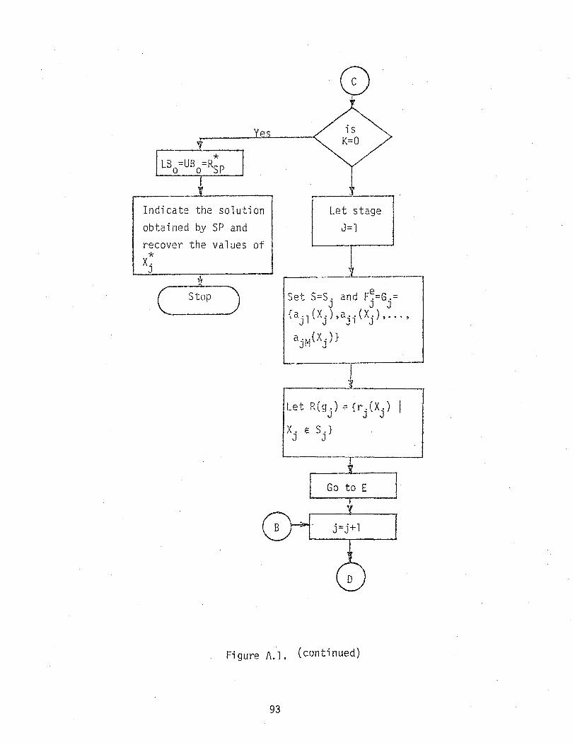
Indicate the solution obtained by SP and recover the values of * x. J
0 I
Let stage ! . J=l
Let R(g .) == {r.(X.) J J J
X. E S.} J J
Figure A.l. (continued)
93

Set S=Sj,K=Kj' and 1et the G.={a. 1(x.),a. 2(x.),
J J J J J
. . . , a j ~1 ( X j ) }
I '-----~
Define imbedded state e space as F.=G. oF.
1 J J J-
1 ·--Define the feasible l state space as I Ff -{ ' ' ' ,.. and j -- ~ j I ~ j € r j i
[2j5_(g)} J
~ Deterrni ne the return of the feasible points as r.=r.(g'.)
J J -J'
Define the efficient state space as F~={Ff- all the
J dominated points}
Figure A. 1. (continued)
94

Let KK be the number
of points in Fj
Determine UBl, and UB2
~~"'"-"'-~;e.-JUBl~ = R(g~) + J -J
UB~ = R(g~) + J -J
N I rt(K)
t=j+l
R(B-[B'(g~)]) -J
I_L_e_t~i -R (_~_}_..;) ~-=......;_-_1 ~~-f-UB-1 J-~ o;- ~~J UB2. < LB. l
J . J-
L
i=i+l
Discard all the points R(g~) < 0 from R.
-J - J
Figure A.l. (continued)
95
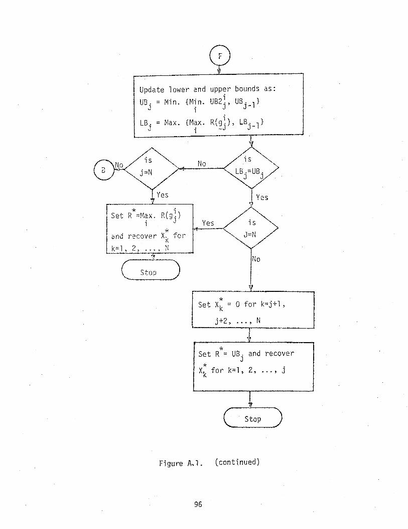
Update lower and upper bounds as: UB. =Min. {Min. UB2~, UB. l}
J J J- . i
LBj = ~1ax. {Max. R(§}), LBj-l} i
Set
and
k= l , 2, ••. , N
No
* Set Xk = 0 for k=j+l,
j+2, ... , N
* Set R = UB. and recover J
* xk for k=l, 2, ... , j
Stop
Figure A~l. (continued)
96

Step 26 - If j=N go to step 28, otherwise go to step 11
Step 27- If j<N, set Xj+l, Xj+2' ... , XN = 0 go to step 29, otherwise
go to step 28.
* R( gj) * Step 28 - Set R = Max and recover xk for k = 1' 2' ••• ' N
and stop.
* * Step 29 - Set R = UB. J
and recover xk for k = 1, 2, ... , j and stop.
Step 30 - Indicate that the solution is obtained by surrogate problem,
* * set R = UB1 and recover \ for k = 1, 2, . . . ' N, and stop .
The information regarding the returns at each stage, and the corres
ponding state space solutions, is stored in a matrix similar to the matrix
TS presented in Section A.2. Similarly, the Tj vectors are used for
* backtracking to obtain the optimal solution ~ .
A.5 Modifications of the Hybrid Algorithm for Large Scale NKP
In order to find a solution to a large NKP, a computationally effi
cient routine must be developed. The hybrid algorithm developed in Section
A.4 provides optimal solutions to medium-size problems in a reasonable
amount of computer time. However, the combinatorial increases in
the state space solution will result in the enumeration of a very
large state variable vector at each stage for large problems even
with the reductions provided by the hybrid algorithm. This causes the
algorithm to require a very large computational time. In this section,
a heuristic procedure is developed and is incorporated in the hybrid
algorithm in order to limit the growth of the state variable vector.
This modification will increase the computational sp~ed and convergence
rate, and reduce the storage required by the algorithm. A mathematical
97

support for the heuristic procedure is demonstrated in the form of a pro
position. This modification suffers from the fact that the solution ob
tained by the modified method may not be an optimum. However, it should
be a good solution to a previously intractable problem.
Preliminary investigation has shown that the increase in the size
of the state variable vector is the primary cause of the increase in
computation time. The size of this vector is a monotonically increasing
function of Kj (number of alternatives in each stage) and N (number of
stages). Therefore, to resolve the problem of slow computational speed,
either N and/or Kj must be kept at reasonably low value(s). In general,
the number of stages N cannot be reduced. However, the value of Kj can
be limited by a systematic approach.
The modification of the hybrid algorithm is based primarily on the
limitation of Kj values. In order to construct a good heuristic proce
dure, consider the monotonicity and separation properties of the objec
tive function. Let ~l =(X~, x1, ... , X~) be any feasible solution to
the following problem:
Problem A. 1
N Max • R ( ~) = z: r • ( X . )
j=l J J
Subject to:
N 2:
j=l a .. (x.) <b.
1J J - 1
X. is contained in S. J J
i=l,2, ... ,M
98

2 2 2 2 Let X = (X1, x2, ... , XN) be an optimal solution obtained from the
surrogated version of the above problem. As discussed in Section A.3~
it is known that the optimal solution to problem A. 1 satisfies the follow
ing relationship:
(A.9)
Thus, a good heuristic procedure would be to find a solution which
falls within the limits defined by A.9. Let s} be a set defined by
1 1 1 X~) 1 2 (X. ' X.+ 1, x.+2, ... for X. <X. s~
J J J J J J =
J X~ 1 2 for X. > X. J J- J
Then the following proposition can be stated:
Proposition: Any feasible point x3 belonging to the set Sj will
have an objective funtion value within the limits defined by F(~ 1 ) as a
satisfactory solution to the original problem, and F(X2) as the optimal
solution of the surrogate Problem A. 1. That is,
(A.lO)
Proof- The following holds true based on the monotonicity and separa
tion properties of the objective function:
(1) By the separation property:
(2) by the monotonicity property:
r . ( X~) > r . ( X~ ) J J - J J
11 xm xn. "' . > J - J
99

~ .
therefore, the following relation holds:
N ~
j=l
m N r (X.) > ~ j J -j=l
r. (X~) J J
m n lJ j where X. > X. J - J
Since any point belonging to s} is greater than or equal to that of
X~ s S ~ and j = 1, 2, ... , N J J
Further, since x2 is the optimal point obtained from a relaxation
(surrogate) of the constraints, any feasible point in s] has the property
that;
N for XJ~ s SJ~ and ~
j=l k a .. (X.) <b.
lJ J - ,
The above proposition has indicated that the choice of S~ will limit J
the variation of the alternative solution and provide a good solution
point if ~l is calculated properly. Algorithm 2 presented in Section
A.3 seems to have the ability of providing such a point. Thus, the only
modification to the hybrid algorithm is to substitute sj for sj.
100

APPENDIX B
PROGRAM DOCUMENTATION OF
RAMS STATE PLANNING PROGRAM
101
-----------------------------

Card
A
'B
c
D
E
F
DESCRIPTION OF INPUT DATA
Column Variable Description
6-65 Title Name of the problem
6-10 NODS No. of districts
11-15 N No. of segments in each districts
16-20 M No. of constraints
21-25 KJ No. of maintenance strategies
26-35 CAPT The capital available in (10,000) dollars
The names of maintenance strategies along with the overhead budget requirements for the strategies. KJ cards are read in.
6-25
26-40
STRT
CR. 1
Strategy Name
Overhead budget requirement for mile-foot
Names of distress type and maximum possible rating for the distress type. ND (number of distress type) cards are read in
6-25
26-40
DSTR Distress type
Maximum possible rating for the distress i
Names of resources types and amounts of resources available per mile-ft. 01-l) cards to be read in.
6-25 RSRC Resource type
26-40 RS. Amount of ith resource 1 available per mile-foot
Resource requirements per mile-foot unit for each strategy.
6-10 L Strategy number
11-17 RSRL 1 1st . resource requ1re-
ments for Lth strategy
102

G
H
18-24
74-80
2nd . t resource requ1remen for Lth strategy
1oth resource requirement for Lth strategy.
The number cards to be read in are KJ. Currently the assumption is that there are at most 10 resources, excluding money.
Potential gains of pavement rating for each distress type. When a certain maintenance strategy is applied. KJ cards are read in. Currently the assumption is that there are at most 10 distress types.
6-10
11-17
18-24
74-80
L
DISTL1
DISTL, 2
DIS\, l O
Strategy number
Gain of rating for the 1st distress when Lth strategy is applied
Gain of rating for theth 2nd distress for the L strategy is applied
Gain of rating for the lOth distress when Lth strategy is applied
Probability of survival for different strategies and distress types for the length of the planning horizon. Length of planning horizon is assumed to be 20 years. (KJ x 20) cards are to be read in. The maximum number of distress types are assumed to be less than 10
6-7
8-10
11-17
74-80
p
L
~1
L,M, 1
p L,M,lO
Strategy number
Year in the planning horizon
Probability of survival for the Lth strategy in Mth year when 1st distress type is present
Probability of survival for the Lth strategy in Mth year when 10 th distress type is present.
Cards type 9, 10, and 11 are associated with each district.
103
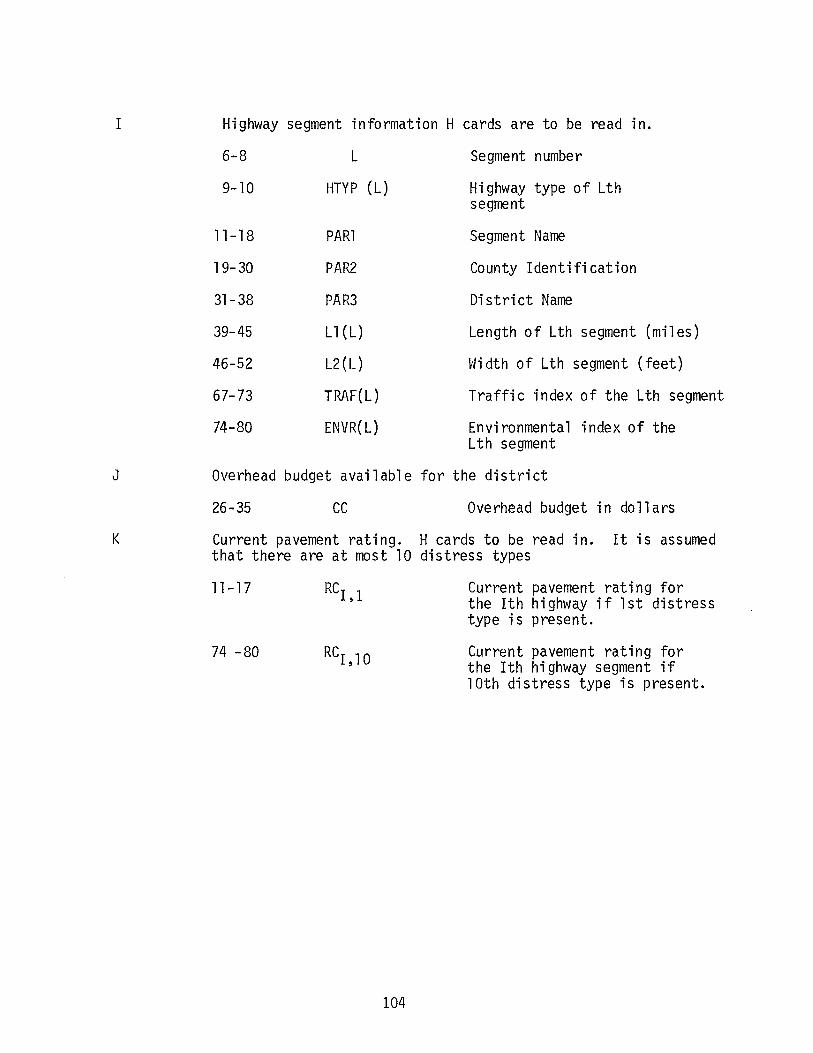
I
J
K
Highway segment information H cards are to be read in.
6-8 L Segment number
9-10 HTYP (L) Highway type of Lth segment
11-18 PARl Segment Name
19-30 PAR2 County Identification
31-38 PAR3 District Name
39-45 Ll(L) Length of Lth segment (miles)
46-52 L2(L) Width of Lth segment (feet)
67-73 TRAF(L) Traffic index of the Lth segment
74-80 ENVR(L) En vi ronmenta 1 index of the Lth segment
Overhead budget available for the district
26-35 cc Overhead budget in dollars
Current pavement rating. H cards to be read in. It is assumed that there are at most 10 distress types
11-17
74 -80 RCI, 10
104
Current pavement rating for the Ith highway if 1st distress type is present.
Current pavement rating for the Ith highway segment if lOth distress type is present.

APPENDIX C
INPUT AND OUTPUT OF
THE EXAMPLE PROBLEM FOR
STATE OPTIMAL FUND ALLOCATION PROGRAM II
105

INPUT DATA
FOR
EXAMPLE PROBLEM
106

0000000001111111111222222222233333333334444444444555555555566666666667 1234567890123456789012345678901234567890123456789012345678901234567890
A STATE OPTIMAL FUND ALLOCATION - PROGRAM II B 3 10 8 6 250
R1 SEAL COAT R2 1.0 INCH OVERLAY R3 2.5 INCH OVERLAY R4 4.0 INCH OVERLAY R5 7.5 INCH OVERLAY R6 10. INCH OVERLAY RUTTING ALLIGATOR CRACKING LONGTUO. CRACKING TRANSVERSE CRACKING FAILURES/MILE SERVICEABILITY INDEX 1\SPHALT CEMENT GRADER LOADER TRUCK GRADER OPERATCR LOADER OPERATOR TRUCK OPERATOR
214.000 950.000 925.000
2ooo.ooo 2600.000 3549.000
1s.ooo 25.000 25.000 20.000 40.000 so.ooo
4.600 0.700 0.340 0.840 0.700 0.340 0.840
c c c c c c 0 D 0 D D 0 E E E E E E E F
F F F F F G
G
G
t o.aoo o.ooo 2 3.000 o.ooo
0.012 o.ooo
0.060 o.ooo 0.278 o.ooo
o.o12 o.o6o o.ooo 0.278
3 I .500 4 4al00 s 8.too
o.ooo o.ooo 0.278 o.ooo o.ooo o.ooo o.ooo 0.556 o.ooo o.ooo o.ooo o.ooo 0.834 o.ooo o.ooo
6 t.5oo o1.ooo o.333 3.611 t.ooo o.333 1 o.ooc 15.000 15.000 15.000 10.000 2.000 2 13.000 19.000 19.000 19.000 24.000 45.000 3 13.000 20.000 20.000 20.000 25.000 45.000
G 4 15.000 25.000 25.000 20.000 30.000 50.000 G 5 15.000 25.000 25.000 20.000 35.000 50.000 G 6 15.000 25.000 25.000 20.000 40.000 50.000 H 1 1 t.ooo t.ooo 1.ooo t.ooo 1.ooo 1.ooo H H H
H H H H H
H
H H
H H H H H
1 1 1 1 1 1 1
2 0.930 3 0.910 4 o.8ao 5 0.780 6 0.310 7 0.220 a o.t5o
1 9 l 10 l 11 1 12 1 13 1 14 1 15 l 16 l 17
0.070 o.oso 0.020 0.020 0.020 0.020 o.oto o.oto o.oto
c.<J40 0.890 0.890 0.650 0.280 0.240 c.t50
Ce930 0.880 0.870 0.670 0.370 0.320 0.180
0.090 0.090 0.070 0.070 0.020 0.020 o.oto o.oto o.o1o o.o1o o.oto o.o1o o.ooo o.ooo o.ooo o.ooo o.ooo o.ooo
107
o.92o t.ooo 0.860 0.910 o.850 0.780 0.670 0.470 0.380 0.2.20 0.330 0.200 0.180 0.100
0.900 0.700 0 .. !:00 0.400 0.300 0.200 o.too
0.090 0.060 o.oto o.oto o.oto o.ooo o.ooo o.ooo o.ooo
o.o40 o.too o.oto o.ooo o.oao o.ooo o.ooo o.ooo o.ooo o.ooo o.ooo o.ooo o.ooo o.ooo o.ooo o.ooo o.ooo o.ooo
0.278 0.556 0.834 3.611

0000000001llllll1112222222222:33333333334444444444555555555566666666667 1234567890123456789012345678901234567890123456789012345678901234567890
H H H H H H H
H H H H
H H H H H H H H
H H
H H H
H
H H H H H
H
H H H H H H H H H H H H H
H H H H H
H
1 18 1 19 1 20 2 1 2 2 2 3 2 4 2 5 2 6 2 7 2 8 2 9 2 10 2 11 2 12 2 13 2 14-2 15 2 16 2 17 2 18 2 19 2 20 3 1 3 2 3 3 3 4
3 5 3 6 3 7 3 8 3 9 3 10 3 11 3 12 3 13 3 14 3 15 3 16 3 17 3 18 3 19 3 20
o.oto o.oto 0.010 1.ooo t.ooo t.ooo t.ooo 0.880 0.780 0.460 0.250 0.250 0.250 o.ooo o.ooo o.ooo o.ooo o.ooo o.ooo o.occ o.ooo o.ooo o.ooo t.ooo 1.000 t.ooo 1.ooo 0.790 0.750 0.750 0.750 0.750 0.750 0.330 0.250 0.250 0.170 o.oeo o.ooc o.ooo o.ooo o.ooc o.ooo
4 1 1.ooo 4 2 1.ooo 4 3 t.ooo 4 4 t.ooo 4 5 t.ooo 4 6 0.830 4 7 0.710
o.ooo o.ooo o.ooo t.ooo t.ooo 0.890 C.820 c.730 0.670 0.670 0.670 0.670 c.360 0.110 0.090 o.ooo o.ooo o.ooo o.ooo o.ooo o.ooo o.ooo o.ooo
o.ooo o.ooo o.ooo t.ooo 1.ooo t.ooo 1.ooo t.ooo 0.750 o.soo 0.500 0.250 o.ooo o.ooo o.ooo o.ooo o.ooo o.ooo o.ooo o.ooo o.ooo o.ooo o.ooo
o.ooo o.ooo o.ooo t.ooo t.ooo 1.ooo 1.ooo t.ooo 0.830 0.670 0.670 0.330 o.ooo o.ooo o.ooo o.ooo o.ooo o.ooo o.ooo o.ooo o.ooo o.ooo o.ooo
o.ooo o.ooo o.ooo 1.ooo t.ooo t.ooo
o.ooo o.ooo o.ooo t.ooo 1.ooo t.ooo
t.ooo o.qoo t.ooo o.aoo 1.ooo 1.ooo 0.330 o.T30 0.330 o.ooo o.ooo o.ooo o.ooo o.ooo o.ooo o.oco o.ooo o.aoo o.ooo
0.700 0.600 0.500 0.400 0.300 o.ooo o.ooo o.ooo o.ooo o.ooo o.ooo o.ooo o.ooo o.ooo o.ooo
1.ooo 1.ooo t.ooo 1.ooo t.ooo t.ooo 1.ooo 1.ooo t.ooo t.ooo o.950 c.930 o.940 t.ooo t.ooo o.9to c.930 o.940 o.890 o.9oo o.9oo o.4oo o.430 o.s3o o.aoo 0.610 0.560 c.550 0.510 0.280 0.170 0.140 0.140 c.t4o o.o8o o.ot o o.ooo o.ooo c.ooo o.ooo t.ooo t.ooo t.ooo t.ooo 0.770 0.640 c.s8o
c.t4o 0.140 0.120 0.070 c.o2o o.ooo o.ooo o.ooo o.ooo o.ooo o.ooo o.ooo o.ooo o.ooo o.ooo t.ooo t.ooo t.ooo t.ooo t.ooo 0.330 0.110
108
0.180 o.tao 0.140 0.060 0.010 o.ooo o.ooo o.ooo o.ooo o.ooo o.ooo o.ooo o.ooo o.ooo o.ooo t.ooo 1.ooo t.ooo t.ooo t.ooo c.630 0.260
0.230 0.160 0.150 0.130 o.oao 0.020 o.ooo o.ooo o.ooo o.ooo o.ooo o.ooo o.ooo o.ooo o.ooo
0.700 0.600 o.soo 0.400 0.300 o.ooo o.ooo o.ooo o.ooo o.ooo o.ooo o.ooo o.ooo o.ooo o.ooo
t.ooo t.ooo t.ooo t.ooo t.ooo t.ooo t.ooo t.ooo 0.770 0.900 0.510 o.soo 0.480 0.700

0000000001111111111222222222233333333334444444444555555555566666666667 1234557890123456789012345678901234567890123456789012345678901234567890
H 4 8 0.660 0.530 0.000 0.220 0.360 0.600 H H H
H H H H H H H H H H H
H H H H H H H H H H H H H
H H
H H H
H H
H H H H H H H H H
H H H H
H H
4 9 4 10 4 11 4 12 4 13
4 14 4 15 4 16 4 17 4 18 4 19 4 20 5 1 5 2 5 3 5 4
5 5 5 6 5 7 5 8 5 9 5 10 5 11 5 12 5 13 5 14 5 15 5 16 5 17 5 18 5 19 5 20 6 1 6 2 6 3 6 4 6 5 6 6 6 7 6 8 6 9 6 10 6 11 6 12 6 13 6 14 6 15 6 16 6 17
0.620 0.380 0.300 0.300 0.300 0.280 0.220 0.170 0.120 0.040 0.040 0.040 t.ooo 1.ooo t.ooo t.ooo t.ooo t.ooo t.ooo 1.ooo t.ooo t.ooo 0.670 0.670 0.670 0.670 0.220 o.ooo o.ooo o.occ o.ooo o.oac 1 .. 000 t.ooo t.ooo t.ooo t.ooo 0.720 0.670 o.sao o.soo 0.500 0.360 0.330 0.330 o.2eo 0.170 0.170 0.170
o.sto c.ooo c.3qo c.ooo 0.210 o.ooo 0.190 o.ooo 0.190 o.ooo 0.170 o.ooo o.tso o.ooo o.too o.ooo o. 070 o. 000 0.060 o.ooo 0.060 o.ooo Oe030 OeOOO t.ooo t.ooo t.ooo .t.ooo .t.ooo t.ooo .t.ooo .t.ooo t.ooo t.ooo o.7to o.330 o.620 o.330 0.440 0.280 0.290 0.170 Oe290 c.290 o.t7o o.t4o Cel40 o.120 o.ooo o.ooo o.ooo o.ooo c.ooo t.ooo t.ooo 1.ooo t.ooo t.ooo c.49o 0.360 0.360 0.360 0.290 c.21o Oe270 0.270 o .. 21o o.21 o c.19o c.t9o
o.t70 c.t 10 0.170 0.170 0.170 0.170 0.110 o.t7o o.1 10 0.170 0.170 1.ooo t.ooo t. 000 t.ooo t.ooo t.ooo t.ooo t.ooo 0.650 0.600 0.600 0.600 c.s3o 0.400 0.380 0.210 Oe200
109
o.tto o.330 o.5oo 0.040 0.240 0.500 o.ooo 0.170 o.ooo o.ooo o.170 n.ooo o.ooo o.t7o o.ooo o.ooo 0.170 o.ooo o.ooo 0.170 o.ooo o.ooo 0.170 o.ooo o.ooo 0.070 o.ooo o.ooo o.ooo o.ooo o.ooo o.ooo o.ooo o.ooo o.ooo o.ooo t.ooo t.ooo 1.ooo t.ooo t.ooo t.ooo t.ooo t.ooo 1.ooo 1.ooo t.ooo t.ooo 1. ooo 1.ooo 1.ooo 0.330 0.750 0.900 0.330 0.590 0.900 o.2ao o.sco n.aoo o.t70 o.soo o.1oo 0.170 0.170 0.170 o.t70 o. 170 o.t70 o.t70 0.170 0.170 o.t7o 0.170 t.ooo t.ooo t.ooo t.ooo t.ooo t.ooo t.ooo t.ooo 0.650 0.600 0.600 0.600 0.510 Oe400 0.380 0.200 o.ooo
0.480 0.250 0.250 0.250 0.250 0.200 o.ooo o.ooo o.ooo o.ooo o.ooo t.ooo t.ooo t.ooo t.oco t.ooo 0.470 0.360 0.320 0 •. 270 0.270 0.270 0.200 0.180 o.tao 0.150 0.090 0.090
0.600 o.ooo o.ooo o.coo o.ooo o.ooo o.ooo o.ooo o.coo o.ooo o.ooo t.ooo 1.ooo t.ooo o.c;oo o.8oo o.7oo 0.600 o.soo 0.400 0.300 o.ooo o.ooo o.ooo o.ooo o.ooo o.ooo o.ooo

0000000001111111111222222222233333333334444444444555555555566666666667 123456 789012345678901234567890123456789012345.6789012345678901234567890
H H H I I I I I I I I I I J K
K
K K K
K K K K K
I I I I I I I I I I J K K
K K K K K
K K K I I I I I
6 18 0.170 6 19 o.t7o 6 20 o.t 70
1 1 DlST 2 lDIST 3 2DIST 4 tDIST 5 1DIST 6 2DIST 1 1DIST 8 lD.IST 9 2DlST
c.t8o c. t 10 0.090
0.200 0.200 0.200
o.ooo o.ooo o.ooo
o.o~o o.ooo 0.090 o.ooo o.oso o.ooo 3.309 36.000 2.266 12.000 3.818 12.000 2.512 12.000 4.712 36.000 1.663 12.000 3.572 24.000 2.462 12.000 2.625 12.000 1.590 12.000 10 lOIST
OVERHEAD BUCGET 705800 1 15.000 25.000 20.000 25.000 30.000 40.000 2 5.000 20.000 20.000 25.000 30.000 o.ooo 3 t5.ooo to.ooo 5.ooo 2s.ooo 3o.ooo 10.ooo 4 5.000 25.000 25.000 25.000 30.000 40.000 5 5.ooo 1o.ooo t5.ooo s.ooo 3o.ooo o.ooo 6 15.000 25.000 15.000 25.000 30.000 40.000 7 15.000 25.000 25.000 25.000 30.000 40.000 8 15.000 20.000 20.000 25.000 30.000 40.000 9 5.ooo 2s.ooo 2o.ooo s.ooo 3o.ooo to.ooo
10 5.000 s.ooo s.ooo 1 lDIST 2 lOIST 3 20IST 4 lOIST 5 1DIST 6 lDIST 7 10IST 8 20IST 9 2DIST
10 101 ST
5.ooo 3o.ooo to.ooo 3.~17 3f:.OOO 2.313 12.000 4.029 12.000 3.356 12.000 3.876 24.000 Le054 12.000 3.439 24.000 3.151 12.000 3.948 24.000 3.331 12.000
OVERHEAD BUDGET 837700 1 s.ooo 1o.ooo 15.ooo 25.ooo 3o.ooo 40.ono 2 15.000 25.000 5.000 25.000 30.000 o.ooo 3 5.000 20.000 25.000 25.000 30.000 40.000 4 s.ooo 25.000 20.000 25.000 30.000 o.ooo 5 t5.ooo to.ooo 2s.ooo 25.ooo 3o.ooo 1o.ooo 6 t5.ooc 25.ooo s.ooo 25.ooo 3o.ooo 4o.ooo 7 15.ooo 25.ooo 2s.ooo 25.ooo 3o.ooo to.ooo a 15.ooc to.ooo 2s.ooo 25.ooo 30.ooo o.ooo 9 15.000 20.000 15.000 25.000 30.000 40.000
10 15.000 25.000 25.000 25.000 30.000 40.000 l lDIST 3.324 36.000 2 lOIST 3 201ST 4 lDIST 5 lDIST
110
2.360 12.000 4.240 12.000 4.200 12.000 3.040 12.000

000000000 llllllllll2222222222.3333333333444 4444444555555555566666666667 1234567890123456789012345678901234567890123456789012345678901234567890
I 6 lOIST 4e445 12 .. 000 I 7 lDIST 3.307 .24.000 l 8 10IST 3.8:39 12 .ooo 1 9 2DIST 1.270 12.000 I 10 lOIST 1.073 36.000 J OVERHEAD BUC<:ET 1002300 K 1 15.000 25.000 25.000 25.000 30.000 o.ooo K 2 15.000 to.ooo 20.000 25.000 30.000 10.000 K 3 15.000 25.000 25.000 25.000 30.000 40.000 K 4 5.000 25.000 20.000 25.000 30.000 40.000 K 5 15.000 20.000 20.000 s.ooo 30.000 40.000 K 6 15.000 25.000 5.000 25.000 30.000 40 .. 000 K 7 5.000 25.000 20.000 25.000 30.0'00 to .. ooo K 8 15.000 25.000 25.000 5.000 .30.000 40.000 K 9 15.000 to.ooo 20.000 25.000 30.000 o.ooo K 10 15.000 5.000 s.ooo 25.000 30.000 40.000
111

OUTPUT OF
EXAMPLE PROBLn1
112

TEXAS TRANSPORTATION INSTITUTE TEXAS A&M UNIVERSITY
COLLEGE STATION, TEXAS 77843
REHABILITATION AND MAINTENANCE SYSTEMS STATE OPTIMAL FUND ALLOCATION - PROGRAM II
BUDGET LEVELS DISTRICT MAXIMUM MINIMUM OPTIMUM BENEFIT
1
2
3
710000
840000
1010000
690000 710000
770000 770000
930000 1010000
2490000
113
2187.
1896.
180 3.
5886.
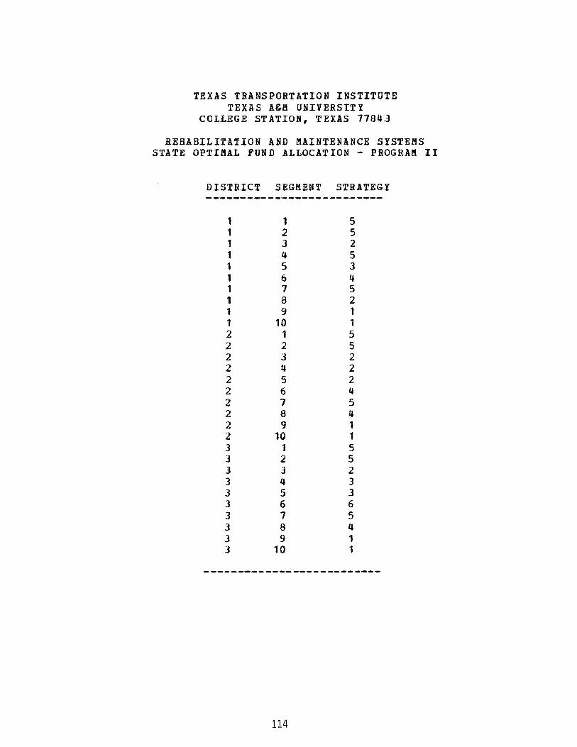
TEXAS TRANSPORTATION INSTITUTE TEXAS A&M UNIVERSITY
COLLEGE STATION, TEXAS 77843
REHABILITATION AND MAINTENANCE SYSTEMS STATE OPTIMAL FUND ALLOCATION - PROGRAM II
DISTRICT SEGMENT STRATEGY
1 1 1 1 1 1 1 1 1 1 2 2 2 2 2 2 2 2 2 2 3 3 3 3 3 3 3 3 3 3
1 2 3 4 5 6 7 8 9
10 1 2 3 4 5 6 7 8 9
10 1 2 3 4 5 6 7 8 9
10
114
5 5 2 5 3 4 5 2 1 1 5 5 2 2 2 4 5 4 1 1 5 5 2 3 3 6 5 4 1 1

APPENDIX D
LISTING OF COMPUTER PROGRAM
115
c c ********************************************************* c C REHABILATATIGN AND MAINTENANCE SYSTEM c C STATE OPTIMAL FUND ALLOCATION - PROGRAM II c C TEXAS TRANSPORTATION INSTITUTE C TEXAS A&M UNIVERSITY C COLLEGE STATICN, TEXAS 77843 c c c c c c c c c c c c c c
AUTHORS
lNSTALLATICN
LANGUAGE
DATE
: EHASHEMI F. TARI CHIYYARATH V. SHA~MUGHAM
: AMDAHL 470V/6 O.ATA PROCESSING CEN.TER TEXAS A&M UNIVERSITV
: FORTRAN IV
: SEPTEMBER .1980
c ********************************************************** c
500 510 520 530 540
COMMON COMMON COMMON COMMON COMMON COMMON COMMON COMMON COMMON COMMON COMMON COMMON COMMON COMMON COMMON INTEGER INTEGER INTEGER REAL FORMAT FORMAT FORMAT FORMAT FORMAT UNIT
/Al/ /A2/ /A3/ /81/ /82/ /83/ /Cl/ /C2./ ./C3/ /C4/ /01/ /El/ /E2/ /F3/ /E4/
NODS, N, M, KJ, CC, CAPT NO, INFIS, UNIT. AICH, TLV, ICHEK, IB. IR Mt, JON, FMAX. lOMAX, L~. LB, UB MIN( 5), MINA( 5), ILOW( 5), NALT( 5) ~AX( 5), MAXA( 5)• IHIG( 5), ZIBR( 5) Bl{ 5t110), Bit{ 5,110), ICY( 5,110), ICZ( 5tl10) IKL(IO), BAR(lO), X(lO) IKU(lO), 100(10), FM(lO) R(l0,6), ICS(t0,8), F(l0,300)• 10{10,300) C(8,10,6), TRACE(500t10t2), 8(8) 15(500)~ TRC(500t2)~ IMS(500,9)~ IMS1(500,9) HTYP(lO). Ll(lO)• L2(10) PAR1{10,2), PAR2(10,3), PAR3(10,2) PAR4(10), PAR5(10), TRAF(lOh ENVR(lO) RC(10.6) CAPT. UNIT, TOTC, x. TRACE TRC, TRCl, TRC2t TRC3• TLV ~TYP. PARlt PAR2, PAR3. D Le, H~S. IMSl, Lt. L2
( 5X. t5A4 ) ( sx. 415. 110 ) ( 5 X • 13, I 2 • 7 A 4, 6F 7 • 3 ) ( 25X. FtO.O } ( lOX. 10F7.3 )
:: 10000 TLV READ WRITE
= tOO (5.500) TITL (6,500) TITL
READ (5.510) NODS, N, Mt KJ, CAPT
116

c
1 2
WRITE (6.510) NODS• ~. ~. KJ. CAPT CALL DATA IN DO 2000 0 = 1• NODS 00 11 0 0 I --= 1 • N READ (5.520) L• HTYP(Ll• ( PARl(L.JJ. J = 1. 2 ).
( PAR2(L.J). J = 1• 3 ). ( PAR3(L,J), J = t. 2 >• Ll{L)• L2(L). PAR4(L), PAR5(L), TRAF(L), ENVR(L)
WRITE (6,520) L, HTYP(L). ( PARl(L.J), J = 1• 2 ), 1 ( PAR2(L.J), J = 1• 3 >• { PAR3(L.J). J = 1. 2 >• 2 Ll(L). L2(L), PAR4(L). PAR5(L)~ TRAF(L). ENVR(L)
1100 CONTINUE
1.200
READ (5.530} cc DO 1200 I = 1 • N READ (5.540) (
WRITE (6.540) (
CONTINUE CALL OBJFCt\ DO 2345 I = 1, N WRITE ( 6.666)
RC(I.Jl. J = t. KJ RC(I,J). J = 1. KJ
WRITE (6,667) ( R(I.J), J = 1, KJ ) WRITE (6,666} DO 1234 J = 1• KJ
)
)
WRITE (6,667) ( C{K,I,J), K = t. M J 1234 CONTINUE 2345 CONTINUE 666 FORMAT ( IX ) 667 FORMAT ( 10F12.5)
ND = D LB=O• UB=O• ZIBR(ND)=O•
C TO CALCULATE THE INITIAL LOWER AND UPPER BCUNOS c
DO 10 J=2.N UB=UB+R ( J • KJ)
10 CONTINUE DO 11 J=l•N 00 11 K=l.KJ S=O. DO 12 I= 1 • M S=S+C(I.J.K)
12 CONTINUE ICS(J.K}=S/M
1l CONTINUE TlB=O• DO 13 I= 1 • M TIB=TIB+B(I)
13 CONTINUE C DO 3456 J = 1, N C WRITE (6,669) ( ICS(J,KJ. K = 1, KJ ) C3456 CONTINUE C 669 FORMAT ( '
IB=TIB/M+t ICS '• 10110 )
C WRITE (6.670) TIB. [8
117

C 670 FORMAT ( ' TIS•, Ft2.3, ' CALL RETRNl I NFS -= 0 CALL SERCHl ( lNFS ) IF ( INFS .ea. 0 ) GO TO 4738 WRITE (6,6E9) NO
IB '• 15 )
689 FORMAT ( ' OJSTRICT'• 13• • IS INFEASIBLE ' ) GO TO 2000
4738 CONTINUE C PRINT,LBeUA
c c c c
c
IF(ICHEK.EO.O) GO TO 15 CALL IMBEDD IOL~=IR
IF(JON.GT.O) GO TO 1000 Z=IMS1(1R,Ml) DO 90 JJ=leN J=N-JJ+l X{J)=TRACE(IR~J,1)
IR=TRACE(IR,Je2) 90 CONTINUE
GO TO 16 1000 Z=IMSl(IReMl)
DO 1001 JJ=leJON J=JON-.JJ+t X(J)-:TRACE(IReJel) IR=TRACE { IR, J ,2)
1001 CONTINUE JON=JON+l
1002
15
60
202
17
DO 1002 JJ=JCN,N X(JJ)=l CONTINUE GO TO 16 Z=FM(N) DO 60 J=l,N X ( J) ·= I OD ( J ) CONT.INUE PRINT 202 FORMAT(20X,•SUROGATE SOLUTION'e//) PRINT 203,Z PR:INT 206 DO 17 Jc=1 ,N PRINT 205tJ,)((J) CONTINUE MAXA(NOl=AICH+l. M INA( ND)=A ICH+l. ZIBR(ND)=-10. BI I(ND,l}-=Z NALT(ND)=l ICZ(ND.1)=l DO 30 .J=ltN ICY(ND,J)=X(J)
30 CONTINUE GO TO 2000
C 16 PRINT 203tZ 16 CONTINUE
118

C 203 FORMAT{20X,•GBJECTIVE FUNCTION VALUE=•,Ft2.5,//) C PRINT 206 C 206 FORMAT(12X, 1 CPT. DEC. VALUE•./)
DO 18 J=t,N C PRINT 205,J.X(J) C 205 FORMAT(12X.I3,12X,I3)
18 CONTINUE IR=IOLP LOC=~ 1-1 MINA(ND):IMSl{l,LOC)+l KOK=MINA(ND) ICZ(NO,t)=KOK-MINA(NO)+l ICY{NO.l)=l BII{ND,tl=IMS(l,Ml) K=l DO 21 J= 1 • IR SUB=IMS1(J,LOC) IF(KOK-SUB) 22,23,23
23 BII(NOeKl=IMSl(J,Ml) GO TO 21
22 KOK=l MSl { J ,LOC) +1 K=K+l ICZ(NO,Kl=KOK-MINA(NO)+l ICY{ND.Kl=J BIICNO.K)=lMSt(J.Ml)
21 CONTINUE NALT(ND)=K MAXA(ND)=ICZ(NO,K)+MINA(N0)-1
2000 CONTINUE UNIT=lOOOO CALL RESULT STOP END
SUBROUTINE COMMON /At./ COMMON /A2/ COMMON /A3/ COMMON. /81/ COMMON /82/ COMMON /83/ COMMON /Cl/ COMMON /C2./ C0'4MON /C3/ COMMON /C4/ COMMON /01/ DIMENSION INTEGER INTEGER REAL
RESULT NODS, N, M, KJe CCe CAPT NOe INFIS, UNIT. AICHe TLVe IC~EK, 18, IR Ml, JONe FMAXe lOMAX, LMe LBe UB MIN( 5h MINA( 5), ILOW( 5>. NALT( 5) N AX ( 5l • MA XA ( 5) • I HI G ( 5) • Z I BR ( 5) 81( 5e110)e Bll( 5e110)e ICY( 5e110)e ICZ( 5ell0l IKL(lO), BAR(lO), X(10) IKU(lO)e 100(10), FM(lO) R(t0,6), ICS(10,8), F(l0,300)e 10(10,300) C(8,10e6), TRACE(500,10t2)• B(E)
15(500), TRC(500,2), IMS(500,9), IMS1(500,9) IY( 5,10) C-PT, UNITe TOTCe Xe TRACE TRC, TRCl, TRC2e TRC3. TLV LB. IMS. IMSl
600 FORMAT ( lHl. //// ) 610 FORMAT ( 51X, 30HTEXAS TRANSPORTATION INSTITUTE, /,
119

c
l 2 3 4
620 FORMAT 1
630 FORMAT 631 FORMAT 635 FORMAT 640 FORMAT
1
(
(
(
(
(
56X• 20HTEXAS A&M UNIVERSITY, /, 52X. 28HCOLLEGE STATION, TEXAS 77843, //, 47X, 38HREHA8ILITATION AND MAINTENANCE SYSTEMS. /, 45X, 42HSTATE OPTIMAL FUND ALLOCATION- PROGRAM ([, // ) 59X, 13HBUOGET LEVELS, /• 44X, 44HDISTRICT MAXIMUM MINIMU~ OPTIMUM BENEFIT •. / 47X, 12• 3X, I9. 19. 19, F9.0., / ) '• 1ox. I9. F9.0J /, 44X, 43( 1 -•), /)
53X, 27HDISTRICT SEGMENT STRATEGY, /• 53X. 26(•-•), / l
650 FORMAT ( 55X. 12w 6X., 12, 8X. 12 ) 660 FORMAT { /, 53X• 26( 9 -•), / )
WRITE {6,600) WRITE (6,610) WRITE ( 6, 620) CAPTN=O• DO 826 I=t.NCOS CAPTN=CAPTN+MINA(IJ
826 CONTINUE CAPT=CAPT-CAPTN+NODS DO 806 I= 1 • NODS NOAL=NALT ( I}
DO 806 J'=l.NCAL
806 C506
PRINT 506.I,ICZ(I.~),BII(I,J) CONTINUE FORMAT(32X.J3,8X.,I8,5X.Ft0.2} INFIS=-99999<;
c c c
DO 4 IN=t,NOOS MAX(IN)=MAXA(INJ-MINA(IN)+l MINCIN)=l CALL RETRt\2(IN)
4 CONTINUE CALL SERCH2
TOTC.=O DO 30 I=t.NODS MIN(IJ=MINA( !)*UNIT MAX(IJ=MAXA(l)*UNIT
OLT PUT
J=IOO(l) ICZ(I,J):(JCZ(I,J)+MINA(I)-l)*UNIT TOTC=TOTC+ICZ(I,J) IF(I.EOel) GO TO 31 11=1-1 RIGH=FM(II} 8I(I,Jl=F~(I)-RIGH
GO TO 32 31 BI(I.J)=FM{I) 32 CONTINUE
WRITE (6,630) I.MAX(IJ.~IN(I),ICZ(I,~).BIII.J)
IF(ZIBR(I).E0.-10.) GO TO 855 IR=ICY( I,J} DO 850 JJ=l•N
120

NIN=N-JJ+l IY(I,NIN)~TRACF.(IR.NIN,t)
IR~TRACE(I~.NIN,2)
850 CONTINUE GO TO 30
855 00 856 J=l•N IY(I,JJ=ICY(l,J)
856 CONTINUE 30 CONTINUE
TOTR=FM(NODS) WRITE (6,~35) WRITE {6.631) TOTC. TOTR WRITE (6,600) WRITE (6,610) WRITE (6,640) DO 1236 I = 1, NODS 00 1235 J = 1• N WRITE (6,650J I, J. IY(I,J)
1235 CONTINUE 1236 CONTINUE
WRITE (6,660) WRITE (6,600) RETURN END
SUBROUTINE COMMON /AI/
COMMON /A2/ COMMON /A3/ COMMON /81/ COMMON /82/ COMMON /83/ COMMON /Ct/ COMMON /C2/ COMMON /C3/ COMMON /C4/ COMMON /01/ INTEGER INTEGER REAL
RETRN2(1) NODS, N, M, KJ, CC, CAPT NO. INFIS. UNIT. AICH, TLV. ICHEK, IBe IR Ml, JONe FMAXe lOMAX. LM, LB. US M IN ( 5 ) • M I NA ( 5 ) , I LOW ( 5 ) • N AL T ( 5 ) ~AX( 5), MAXA( 5)• IHIG( 5), ZIBR( 5) Bl( 5,110), Bill 5,110), ICY( 5,110), ICZ( 5,110) I KL ( 1 0 h BAR ( 1 0 ) , X ( 1 0) IKU(lO), IOD(lO), FM(lO) R(10,6}, ICS(t0,8), F(t0,300), 10(10,300) C(8,t0,6), TRACE(500.t0.2l• 8(8) 15{500), TRC(S00.2), IMS(500,9), IMS1{500,9) CAPT, UNIT. TOTC. x. TRACE TRC, TRCt, TRC2, TRC3, TLV LB. I MS, IMSt
IF{I.GT.t) GC TO 3 KK=MAX( I) ISS=MIN(l)-l NOAL=NAL T ( l ) K=MlN(I)-1 IF(NOAL.EOel) GO TO 40 NIL=NOAL-1 GO TO 41
40 NIL=l 41 DO 2 JOZ=leNIL
K01=ICZ(I,JOZ) JOZY=JOZ+l
121
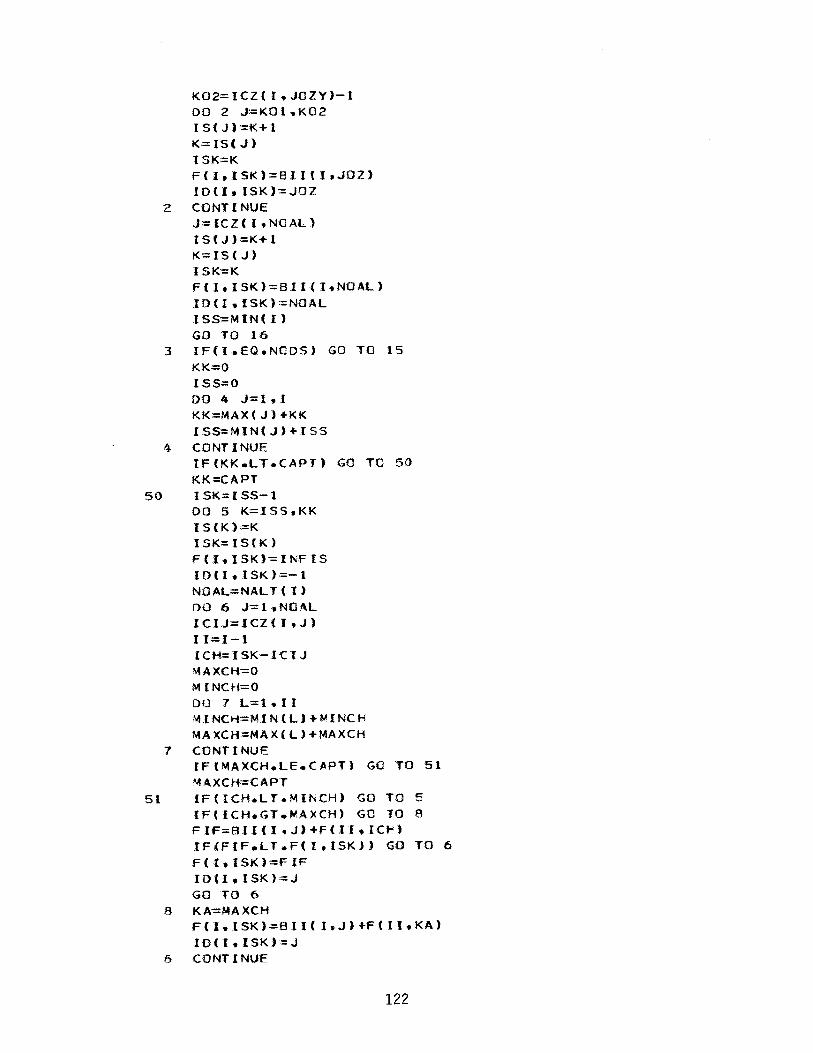
50
51
K02=ICZ( 1-.JOZY)-l DO 2 J-=K01-.K02 IS(J)::K+l K=IS(J} ISK=K F(I-.ISK)=EII(J-.JOZ) ID(I.ISK)=JOZ
2 CONTINUE J = l C Z ( I -. NO .AL ) IS(J):K+l K=IS(J) ISK=K F(I.ISK)=BIICI-.NO.AL) ID( I -.ISK) ::NOAL ISS=MIN( I) GO TO 16
3 IF(I.EOeNODS) GO TO 15 KK=O ISS=O DO 4 J=l•I KK=M.AX(J)+KK ISS=MIN(J)+ISS
4 CONTINUE
7
8
lF(KKeLTeCAPT) GO TO 50 KK=CAPT I SK=I SS-1 DO 5 K=ISS-.KK I S(K):=K ISK=IS(K) F(l-.ISK)-=lt\FIS 10(1-.ISK)-=-1 NO.AL=NALT ( I) DO 6 J=l -.NOAL ICIJ=ICZ(I-.J) JJ:I-1 ICH=ISK-ICIJ MAXCH=O M INCH=O DO 7 L=l-.11 MINCH=MIN(L)+MINCh MAXCH=MAX(L)+MAXCH CONTINUE IF(MAXCH.LE.CAPT) GO TO MAXCH=CAPT IF( ICH.LTeMINCH) GO TO IF(ICH.GT.N!AXCH) GO TO FIF=Bil(l-.J)+F(ll-.IC~)
IFCFIFeLT.F(l-.ISKJ) GO F(l-.ISK)=FIF I D (1 • I SK ) -= J GO TO 6 KA-=MAXCH
51
5 8
TO
F{I.ISKJ=BIICI-.J)+F(II-.KA) 10(1-.ISK)=J
6 CONTINUE
122
6

5 CONTINUE GO TO 16
15 CONTINUE NOAL=NAL T ( I)
DO q .J= 1, NOAL IF(CAPT.GT.300) GO TC 61 ISK=CAPT GO TO 62
61 ISK=249 CAPT=ISK
6 2 F ( I. I SK) ·= I NF I S IDU.ISKl=-1 II=I-1 ICI.J-=ICZ( I,J) ICH=ISK-ICI.J MAXCH=O MINCH.:::O 00 11 L=l,II MINCH=MINCL )+t.!INCH MAXCH=MAX(L)+MAXCH
11 CONTINUE IFIMAXCH.LE.CAPT) GO TO 52 MAXCH=CAPT
52 IF(JCH.LT.~INCH) GO TO 9 IF(lCHeGTeMAXCH) GO TO 12 FIF=B.Il(l,.J)+F(Il,ICh) IF(FIF.LT.F(I,ISK)) GO TO 9 F(I,ISK)==FIF IO(I,ISKl=J GO TO 9
12 KA=MAXCH F(I.ISK)=BII(I,Jl+F(li,KA) ID(I.ISK)=J
9 CONTINUE 16 ILOW( Il=ISS
I HIG( I )=KK RETURN END
SUBROUTINE COMMON /AI/ COMMON /A2/ COMMON /A3/ COMMON /81/ COMMON /82/ COMMON /83/ COMMON /Cl/ COMMON /C2/ COMMON /C3/ COMMON /C4/ COMMON /01./ INTEGER.
SERCH2 NODS, N. M, KJ, CC, CAPT 1\0, INFIS• UNIT, AICH. TLV, ICHEK, IS, IR Mt, JON, FMAX, lOMAX, LM, LE. UB MIN( 5), MINA( 5), ILOW( 5), NALT( 5) MAX( ~) • MAXA( 5) • IHlG( 5), ZIBR( 5) 81( 5,110), BII( 5.110)• ICY( 5,110), ICZ( 5,110} I KL ( 1 0 t • BAR ( 1 0 ) • X ( 1 0 ) lKU(lO), 100(10), FM(lO) R(t0,6), ICS(t0,8), F(10,30Q), 10{10,300) C(9,tO,E), TRACE(500,10,2), 8(8) 15(500), TRC(500,2), IMS(500,9), IM$1(500,9) CAPT, UNIT, TOTC. x~ TRACE
123

INTEGER REAL Jc=NOOS
TRC, TRCI, TRC2• TRC3, TLV LB, IMS, .1"451
F M ( I ) =F ( I • C APT } IOO(J):IO(I,CAPT) J:IOO(l) KEK=NODS-1 ISIS=CAPT-ICZCI,J) 00 2 I=ltKEK JI:NOOS-.1 IF(ISIS.GT.IHIG(ll)) GO TO 3 K=IS.IS FM (I I )c::F ( I I t K ) IOO(IIl=IDCJI.Kl J=IOD(If) ISIS=ISIS-ICZ(lltJl GO TO 2
3 K:JHIG{ll) FM {I I )=F (I 1 ,I<)
IOD{IIJ=IO(II,K) J=IOD(II) ISIS=ISIS-ICZ(II.J)
2 CONTINUE RETURN END
SUBROUTINE COMMON ./Al/ COMMON /A2./ COMMON /A3./ COMMON /Bl/ COMMON /82/ COMMON ./83/ COMMON ./Cl/ COMMON /C2./ COMMON /C3/ COMMON /C4/ COMMON /01./ INTEGER INTEGER REAL FMAX=O•
RETRNt NODS, N, M, KJ, CC, CAPT ~C. INFISt UNIT, AICH, TLV. ICHEKt IB, IR Mt, JON, FMAX, IDMAX. LM, LBt UB MIN( 5), MINA( 5). ILOW{ 5), NALT( 5) MAX( 5), MAXA( 5), IHIG( 5), ZIBR( 5) 81( 5,110), BII( 5tl10), ICY( 5.110), ICZ( 5,110} IKL(lO), BAR(tO), X(lO) IKU(lO), 100(10), FM(lO) R(10,6lt ICS{lO,S), F(10t300), 10(10.300) CC8.10t6), TRACE(500tl0t2l. 8(8) 15(500), TRC(500,2), IMS(500t9), IMS1(500t9) CAPT, UNIT, TOTC, X, TRACE TRC, TRClt TRC2. TRC3t TLV LBt H~S. IMSl
LM - 0 IF ( IB .LE. 300 ) GO TO 1200 WRITE ( 6,667) 18 = 300
1200 CONTINUE 667 FORMAT ( • **** 18 GT 300. SET 18 = 300' )
DO 11 J: 1 eN DO 11 L:t,I8 ID(J,L)=l F(J,L)=-999.
124

DO 12 K=t~KJ ICSI=ICS{J,Kl ISL=L-1 IF{ISL.LT.ICSI) GO TO 11 IF(J.GT.1) GO TO 13 FI=R(J~K)
GO TO 14 13 JJ=ISL-ICSI+1
JK=J-1 FI=R(J,K)+F(JK~JJ}
14 IF(FI.LT.F{J.L)) GO TO 12 F{J,L)=FI ID(J,L).=K
12 CONTINUE IF(J.LT.N) GO TO 11 IF(FMAX.GE.F(J,L)) GO TO 11 FMAX=F(,J.L) IDMAX=IO(J,L) L M:::L
11 CONTINUE C DO 1234 L::: It IB C WRITE (6,777) ( ID(J,L), J = 1• N ), ( F(J,L), J = t, N ) C1234 CONTINUE C 777 FORMAT ( 1015, 10F7.1 ) C WRITE (6,778) LM C 778 FORMAT ( 1 LM '• 15 )
IF ( LM aGT. 0 ) RETURN WRITE (6,666) LM
666 FORMAT ( 1Xt '?????????????? LM IS '~ 13 ) STOP END
SUBROUTINE COMMON /Al/ COMMON /A2/ COMMON /A3/ COMMON /81/ COMMON /82./ COMMON /83/ COMMON /Ct/ COMMON /C2/ COMMON /C3./ COMMON /C4/ COMMON /01./ INTEGER INTEGER REAL IND=O
16 LM=LM-INO KK=ID(N.LM)
SERCHl ( lNFS ) NODS, N, M, KJ, CC, CAPT NO, INFIS, UNITt AICHt TLV, ICHEK. IB, IR M1, JON, FMAX, lOMAX, L~. LB, UB MIN( 5), MINA( 5), lLOW( 5), NALT( 5) MAX( 5) • MAXA( 5} • IHIG( 5h ZIBR( 5) 81( 5,110), 811( 5t110), ICY( 5,110), ICZ( 5,110) IKL(lO), BAR(lQ), X(lO) lKU(lO), 100(10), FM(10) R(l0,6), ICS(10t8lt F(10,300), 10(10.300) CC8.t0,6)• TRACE(500.t0.2)t 8(8) I S { 50 0 ) , TR C ( 50 0 • 2 ) , I M S ( 50 0 • 9 ) • I MS 1 {50 0 • 9) CAPT, UNIT. TOTC. X, TRACE TRC, TRCl, TRC2. TRC3, TLV L8, IMS, lMSt
F M ( N ) =F ( N , U~ l IOD{N)=ID(I\,LM)
125
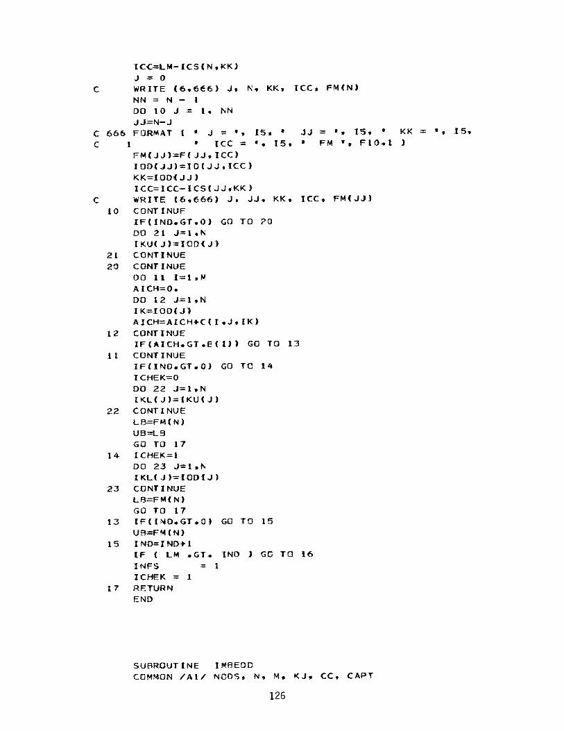
ICC-=LM-ICS(N,KK) J = 0
C WRITE (6,666) J, N. KK. ICC. FM(N) NN = N - l DO 10 J :::: 1. NN JJ:::N-J
C 666 FORMAT ( • J = •, C 1 • ICC =
15. • JJ = •• 15 •• '• 15, ' FM '• FtO.t
FM(JJ)=F(JJ.ICC) IOD(JJ)=ID(J~.ICC)
KK=IOD(JJ) ICC=ICC-ICS(JJ.KK)
c WRITE (6.666) J. J.J. KK. ICC. FM(JJl 10 CONTINUE
1F(IND.GT.O) GO TO ?0
00 21 J=l,N IKU(Jl=IOO(J)
21 CONTINUE 20 CONTINUE
DO 11 I=l• M AICH=O. DO 12 J=1,N IK=IOO(J) AICH=AICH+C(I.J.IK)
12 CONTINUE IF(AICH.GTeE(I)) GO TO 13
1 1 CONTINUE IF(INO.GT .. O) GO TO 14 ICHEK=O DO 22 J=l•N IKL(J)=IKU(J)
22 CONTINUE LB=FM(N) UB-=LB GO TO 17
14 ICHEK-=1 DO 23 J=l,N IKL(J)=IOO(J)
23 CONTINUE LB=FM(N) GO TO 17
13 lF{l1140eGT.Ol GO TO 15 UB=FM(N}
15 I NO= I ND+l IF ( LM eGTe INO ) GO TO 16
INFS ·- 1 ICHEK :::: 1
17 RETURN END
SUBROUTINE IMBEDD COMMON /Al/ NCDS. N, M, KJ, CC. CAPT
126
KK = '• I 5. )
COMMON /A2/ COMMON /A3./ COMMON /Bl/ COMMON /82/ COMMON /83/ COMMON /Cl/ COMMON /C2/ COMMON /C3/ COMMON /C4/
COMMON /01/ .INTEGER INTEGER REAL J=l JON=O UCB=UB DO 10 K=l,KJ IR=K
ND. INFIS, UNIT. AICH, TLV, ICHEK, IB. IR ~~. JON, FMAX, IDMAX. LM• LE. UB MIN( 5)• MINA( 5), ILOW( 5), NALT( 5) MAX{ 5), MAXA( 5), IHIG( 5), ZIBR( 5) BI( 5,110), 811( 5,110), ICY( 5,110), ICZ( 5,110} IKLC10), 8AR(10), X(lO) IKU{lQ), 100(10), FM(10) R(t0,6). ICS(t0,8), F(l0,300), 10(10.300) C(8,t0,6), TRACE(500,10,2), 8(8) 15(500), TRC(500,2), IMS(500,9), IMS1{500,9) CAPT, UNIT, TOTC, X, TRACE TRC. TRCt, TRC2. TRC3, TLV LE, IMS, IMSl
DO 11 1=1• M IMSICK.IJ=CCI.J,K) IMS(K,Il=C(I,J.K)
t 1 CONTINUE Ml=M+l IMSl(K.Ml)=R(J,K) IMS(K,Mt )=fHJ,K) TRC(IR.l}=l< TRC(IR,2)=1 TRACE( IR, 1 ,1 }::K TRACE( IR • 1.2 ):::1
10 CONTINUE DO 12 J=2,N DO 18 IRR=l.IR TRC(IRR.1).:1 TRC(IRR,2}=1RR
18 CONTINUE IRB=IR TLILY=IMSl(IR.Ml) TLILI=IMS1(IR,M) IRM=IR KJU=IKU(J) KJL=IKL(JJ IF(KJL.EQ.t) GO TO 3 IF(KJU-KJL) 2.2.4
2 KJU=KJL GO TO 4
3 KJL=2 IF(KJU.GE.2) GO TO 4 GO TO 76
4 DO 13 K=KJL,t<JU 00 14 L=l.IRM
c C FEASIBILITY TEST c
DO 99 l=l•M F IS I B-= I MS 1 ( L • I H·C ( I • J • K)
127

c
1F(FISIB.GT.8(1)) GO TO 14 99 CONTINUE
lF(J.EO.N) GO TO 85 RTl=IMSl(L.Ml)+R(J.K) JK=J+l UBI=RT1 DO 15 JJ=JK.tUBl=UBl+R(..JJ .I<J)
15 CONTINUE TMSR=O• DO 16 1=1 .M TMSR=TMSR+ I MS 1 (L • I )+C (I • J ,K)
16 CONTINUE IMSR=TMSR/M LL=IB-IMSR UB2=F< N.LL )+RTl
C THE LOWER BOUND TEST c
c
IF(UBt.LT.LB) GO TO 14 IF(UB2.LT.LB) GO TO 14
C TO UPDATE THE UPPER BOUND c
c
IF(UB2.GT.UB) GO TC 85 UB=UB2
85 I RB=IRB+l
C TO CONSTRUCT Tt"E IMBEDDED STATE VECTOR c
00 17 1=1,M IMSCIRB.I)=IMSt(L,I)+C(I,J.Kl
17 CONTINUE IMS(IRB,Mll=IMS1(L.M1)+R(J,K) TRC(IRB,l)=K TRC(IRB.2)=L
14 CONTINUE 13 CONTINUE
I R=IRB IF(J.EO.NJ GO TC 50 IF{IR.LT .TLV) GD TO 76
50 DO 19 JRR=1.1R NI=IR-IRR+l B 0 Z= I MS ( l • M 1 ) JAK=l IF(NI.EQ.l) GC TO 19 DO 21 IRC=2.f\l lF{IMS(IRC.Ml).LTeBCZ) GO TO 21 BOZ=I MS( lRC. M l) TRCl=TRC( .IRC .1) TRC2=TRC( IRC.2) DO 40 1-=l,Ml BAR(I)=lMS(I~C.Il
40 CONTINUE JAK=IRC
128

c
21 CONTINUE DO 22 I=l,Ml IMS(JAK,I)=I~S(NI,I)
I MS( N I • I) =EAR (I) 22 CONTINUE
00 23 f:=l .2 TRC(JAK.IJ=TRC(NI.I)
23 CONTINUE TRC(NI,l)=TRCl TRC{Nle2)=TRC2
19 CONTINUE IF(J.EQ.N) GC TO 76
C DOMINANCY TEST c
00 24 IRR=2.IR IFCIMS{IRR,Mtl.LT.-1.) GO TO 24 IRI-=IRR-1
39 IF(lMS(IRt,Mt).GT.O) GO TO 45 IF(IRt.EQ.l) GO TO 24 IRl=IRl-1 GO TO 39
45 IF(IMS(IRl,Ml)-IMS(IRR,Mt)) 25,26,24 25 DO 28 I=leM
IF(IMS(IRR,IJ-IMS(IRlel)) 28,28,24 28 CONTINUE
IMS(IRl,Ml)-=-~99.
IF(IRl.EO.l) GO TO 24 IRl=IRl-1 GO TO 39
26 ICH1=0 I CH2=0 DO 31 I= l • M IF(IMS(IRRei)-IMS(JR191)) 32,33934
32 I CHI-= 1 GO TO 31
34 ICH2=1 GO TO 31
33 ICH3=ICHI*ICH2 IF(ICH3.EQ.O) GO TC 31 GO TO 24
31 CONTINUE ICH3=ICHl*ICI-'2 IF(ICH3.EQ.t) GO TO 24 IF(ICHleEO.O) GO TO 35 IMS(IRleMl)=-~99.
IF(IRt.EQ.l) GO TO 24 IRl:JRl-1 GO TO 39
35 IMS(IRR,Ml)=-999. 24 CONTINUE
IF(J.EQ.N) GC TO 76 JAHL=J+l IRM=IR IRMl=IR
129

DO 88 L= t • IRM IF(IMS(L.Mt).LT.O.) GO TO 88 TOKH=O• 00 77 JJ=JAHt..N TOKH=JMS(L.M1)+R(JJ.KJ)+TOKH
77 CONTINUE IF(TOKH.GE.LB) GO TC 76 IMS(L,Ml }c=-999.
88 CONTINUE 76 111=0
IF(IR.GT.O) GC TO 200 GO TO 300
200 I RIM= 1 IF(IReLTeTLV) GO TO 201 HHM=IR-TLV+l
201 00 36 IRR=lRI~.IR IF(IMS(IRR.Mt).LT.O) GO TO 36 III-=III+l DO 37 I=l• t-'1 I~Sl(III.I)=IMS(IRR.I)
IMS(III.I}:It-'Sl(III.I) 37 CONTINUE
DO 38 1=1.2 TRACE(III.J.Il=TRC(IRR.I)
38 CONTINUE 36 CONTINUE 6 IR=III
IF(III.EO.O) GO TC 1002 C PRINT.ND.J.IR.IMSl(III.Ml)
LIIB=IMSltiii.Ml) c C TO UPDATE THE LOWER BOUND c
c
IF(LIIB.LEeLB) GO TO 12 LB=LI IB
C TERMINATION TEST c
IF(LB.GE.UB) GO TO 1000 12 CONTINUE
GO TO 1001 1002 IR=IRM
IMSl(IR,Ml}=TLILY LILA=Ml-1 IMSl(IR,LJLA}:TLILI
300 JON=J-1 GO TO 1001
1000 IF(J.EQ.N) GO TO 1001 JON-=J
C1001 PRINT.UB 1001 CONTINUE
RETURN END
130

500 510 520
SUBROUTINE CAT AIN COMMON COMMON COMMON COMMON
/At/ /Fl/ /F2/ /F3/
~ODS. N. NC. NS. CC. CAPT STRT(6.5), DSTR(6.5), RSRC(10,5) CR{6), R~AX(6), RS(lO), RSR(6,10) OIST(6,6), P(6,20.6)
COMMON INTEGER Mt FORMAT FORMAT
/Gl/ T. NPAN. NTYP
(
(
T
- NC - 1 5X, 5A4. Fl5.3 ) !: X, 15 • 1 OF7 • 3 )
FORMAT NO
( 5 X " I 2 • .13 • 1 OF 7 • 3 )
= 6 NTYP .: 2 T = 10 NPAN = 20 DO 1200 I = 1• NS READ (5,500) ( STRT(I,J), WRITE (6.500) ( STRT(I,J),
J ..J
- t. 5 ) . CR (.I)
= t. 5 ) . CR(I) 1200 CONTINUE
DO 1300 I = t, NO READ (5,500) ( DSTR(I,J), WRITE (6,500} ( DSTR(I,J),
1300 CONTINUE DO 1400 I = t, Ml READ (5.500) ( RSRC(I.J), WRITE (6,500) ( RSRC(I,J),
1400 CONT.INUE DO 1500 I = 1, NS
J = .J =
J ·-J =
1. 5 ) . RMAX(I) t • 5 ) . FiMAX(I)
1 • 5 ) . RS( I} 1. 5 ) . RS(l)
READ (5.510) L• { RSR(I.J), J = 1• Mt ) WRITE (6.510) L
1500 CONTINUE DO 1600 I = 1• NS READ (5.510) L, ( DIST(I,J), J = l• ND ) WRITE (6,510) L
1600 CONTINUE DO 1800 I = t, NS DO 1800 J = 1, NPAN READ (5,520) L, M. ( P(L,M,K). K = t, NO ) WRITE (6,!:20) L• M
1800 CONTINUE RETURN END
SUBROUTINE COMMON /Al/ COMMON /A2/ COMMON /C3/ COMMON /C4./ COMMON /El/ COMMON /F2/
OBJFCN NODS. N. M• NS, CC. CAPT NO. INFIS. UNIT, AICH, TLV. ICHEK~ IB. IR R(10,6). ICS(\0,8), F(10,300l. 10(10.300) C(8,t0,6), TRACE(500.t0.2). 8(8} HTYP(lO). Ll(lO), L2(10) CR(6). RMAX(6)• RS(lO), RSR(6,10)
131

2000
2100
3100
3700 4000
2500
COMMON /Gl/ T-. NPAN-. NTYP DIMENSION XL(lO) INTEGER .T • UNIT REAL L 1-. L2 Ml -- M - 1 XXL - o.o 00 2000 I - 1 • N XL(I) = L 1{ l) * L2(1) XXL = XXL + XL( I) CONTINUE DO 2100 I = 1. Ml RS(l) = PS(I) * XXL 8( I) = 70.000 CONTINUE 804) = cc / UNIT 00 4000 I -- 1 • N
INOX = 0 DO 3700 J = 1 .. NS CALL BENFIT { 1-. J. SUM )
R{l-.J} -- SUM * XL( I) / 100.0 XSGR -= o.o DO 3100 K - 1 • Ml C(K.I-.J) = too.o * XL( I) * RSR(J-.K) CONTINUE C{M-.1-...J) -- ( XL( I) * CR(J) ) / UNIT CONTINUE CONTINUE RETURN END
SUBROUTINE EENFIT ( 1-. J-. SUM ) COMMON /At/ NODS-. N. M-. NS-. CC-. CAPT
/ RS(K}
COMMON /C3/ R(l0-.6)-. ICS(lO-.R)-. F(l0-.300)-. lD(l0-.300) COMMON /E3/ PAR4(10}-. PAR5(10), TRAF(lO)• ENVR(tO) COMMON /E4/ ~<(10.6) COMMON /F2/ CR(6)-. RMAX{6), RS(lO)-. RSR(6-.10) COMMON /F3/ DIST(6-.6)-. P(6.20-.6) COMMON /Gl/ T-. NPAf\-. NTYP INTEGER T REAL SUM DO 3000 L IT DTJK RR CONT.INUE L ;:>p
pp
IF ( RR IF ( pp
Ll-. L2 - o.o
K - 1-. NS - 0 = T = AMINl(DIST(J.K)-.RMAX(K)-RC(l-.K)+O.l) - RC{l-.K) + DTJK
- L + 1 - l-.0- TR~F(I) * ENVR(l) * ( 1.0- P(J.L.K) ) = AMAXl(O.O-.PP*RMAX(K))
~LT. PP ) GO TO 2600 .LT• RC(I-.K) ) GO TO 3000
132

SUM = SUM + PP- RC(l.K) IF ( SUM .LE. o.o ) SUM = 0.0 GO TO 2700
2600 IT = IT + 1 2700 IF ( IT .GE. NPAN ) GO TO 3000
IF ( L .LT. IT ) GO TO 2500 3000 CONTINUE
RETURN END
133