reinforcement learning 2 slides

Artificial Intelligence: Representation and Problem

Solving

15-381

May 3, 2007

Reinforcement Learning 2

Michael S. Lewicki ! Carnegie MellonArtificial Intelligence: Reinforcement Learning 2

Announcements again

• Don’t forget: fill out FCE’s

www.cmu.edu/fce

• Review session for final:

Tuesday, May 8

6:00 - 8:00 pm

Wean 4623

2


Reinforcement learning so far

• Goal is the same as MDPs: discover policy that maximizes reward

• But, unlike MDPs, we don’t know: state space (world), transition model, or reward function

- only know what state you’re in and the available actions

• Need to explore state space to discover best policy

• Model estimation:

- do a set of trials (each that runs until a terminal state is reached)

- estimate the rewards and a transition probabilities using the counts across trials

• Now use estimates in MDP policy estimation techniques

3

?

??

?

T (s, a, s′) = ?R(s) = ?

3

2

1

1 2 3 4


Evaluating value function from estimates

• Problem: how long do we wait before estimating V(s) (in order to estimating policies)?

• If we want to adapt our policy or use it for more efficient exploration, we need to have an up-to-date estimate

• Estimating V(s) is expensive if done at each iteration.

• Ideas for improvement:

- “one backup” only update the value estimate for state si (ie one state back) instead of all

- Prioritized sweeping: use priority queue to update states with large potential for change

4

?

??

?

T (s, a, s′) = ?R(s) = ?

3

2

1

1 2 3 4


Direct estimation of the value function

• Note, that we could also use the trials to estimate the value function directly:

- at the end of each trial, calculate the observed future reward for each state

- get estimates for V(s) for each state by averaging over trials, and multiple visits within a trial.

• Also called Monte Carlo estimation, since it samples randomly using the policy !(s).

• Utility of each state equals its own reward + the expected utility of successor states:

• But, this is also inefficient than the other methods and learning only occurs at the end of each trial.

5

?

??

?

T (s, a, s′) = ?R(s) = ?

3

2

1

1 2 3 4

V (s) = R(s) + γ∑

s′

T (s,π(s), s′)V (s′)


Temporal distance learning

• After each trial we will have noisy estimates of the true values V(s)

• Consider transition (3,2) "(3,3) and its two noisy estimates.

• What value do we expect for V(3,2)?

V(3,2) = -0.04 + V(3,3)

= -0.04 + 0.94 = 0.90

• The observed value is lower than the current estimate, so V(3,3) is too high.

• Why don’t we adjust it to make it more consistent with our new observation?

6

3 0.85 0.94

2

1

1 2 3 4

two current estimates of V(s)

3 0.812 0.868 0.912 +1

2 0.762 0.660 -1

1 0.705 0.655 0.611 0.388

1 2 3 4

true values of V(s)


• For any successor state s’, we can adjust V(s) so it better agrees with the constraint equations, ie closer to the expected future rewards.

• Note: this doesn’t involve the transitions T(s,a,s’). We only update the values V(s).

• Not quite as accurate as earlier methods, but:

- much simpler and requires much less computation

• Why “temporal” ? In terms of a state sequence:

Temporal difference learning

7

current value

expected future reward

New estimate is weighted sum of

V̂ (s) ← (1− α)V̂ (s) + α(R(s) + γV̂ (s′))= V̂ (s) + α(R(s) + γV̂ (s′)− V̂ (s))

current value

difference between current value and new estimate after

transitioning to s’.

The TD (or temporal difference) equation

+

V (st)← V (st) + α [Rt + γV (st+1)− V (st)]


TD algorithm

1. initialize V(s) (arbitrarily)

2. for each trial

3. initialize s

4. for each step in trial

5. observe reward R(s); take action a = !(s); observe next state s’

6.

7.

8. until s is terminal

8

V (s)← V (s) + α [R(s) + γV (s′)− V (s)]

s← s′


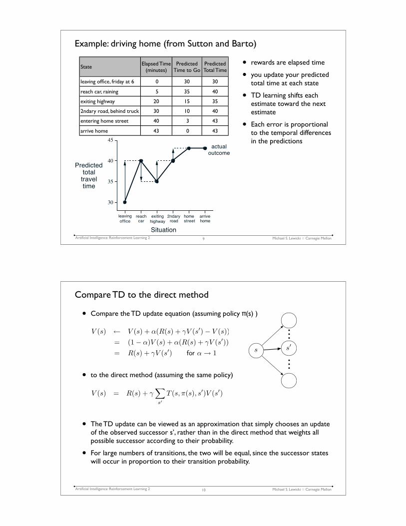
Example: driving home (from Sutton and Barto)

9

StateElapsed Time

(minutes)Predicted

Time to GoPredictedTotal Time

leaving office, friday at 6 "0 30 30

reach car, raining "5 35 40

exiting highway 20 15 35

2ndary road, behind truck 30 10 40

entering home street 40 "3 43

arrive home 43 "0 43

actualoutcome

Situation

30

35

40

45

Predictedtotaltraveltime

roadleaving

officeexiting

highway

2ndary home arrivereachcar street home

• rewards are elapsed time

• you update your predicted total time at each state

• TD learning shifts each estimate toward the next estimate

• Each error is proportional to the temporal differences in the predictions


• Compare the TD update equation (assuming policy !(s) )

• to the direct method (assuming the same policy)

• The TD update can be viewed as an approximation that simply chooses an update of the observed successor s’, rather than in the direct method that weights all possible successor according to their probability.

• For large numbers of transitions, the two will be equal, since the successor states will occur in proportion to their transition probability.

Compare TD to the direct method

10

V (s) ← V (s) + α(R(s) + γV (s′)− V (s))= (1− α)V (s) + α(R(s) + γV (s′))= R(s) + γV (s′) for α→ 1

V (s) = R(s) + γ∑

s′

T (s,π(s), s′)V (s′)

• • •• • •

s s′


The temporal difference equation

• How do we choose # (the learning rate)?

• It’s a weighted sum, so 0 < # < 1.

• Too small: V(s) will converge slowly, biased toward current estimate

• Too large: V(s) will change too quickly, biased toward new estimate

• Decaying learning rate strategy: start large when we’re not sure, then reduce as we become more sure of our estimates, eg #t = 1/t.

11

∞∑

t=1

αt =∞

∞∑

t=1

α2t <∞

Theorem: for V(s) to converge to

correct value #t must satisfy:

V (s)← V (s) + α(R(s) + γV (s′)− V (s))

t

!t


What about policies?

• Previously, we estimated the policy using MDP approaches, e.g. via value iteration

• But, this involves estimating the transition model, which is expensive.

• Can we do it without?

12

π∗(s) = arg maxa

[R̂(s) + γ

∑

s′

T̂ (s, a, s′)V ∗(s′)

]


Q-learning

• Idea: Learn an action-value function that estimates the expected utility of taking action a in state s.

• Define a state-action pair: Q(s,a)

- value of taking action a at state s

- best expected sum of future rewards after taking action a at state s

• This is like the value function before, except with an associated action a:

• The max over actions defines the best over all possible succeeding states.

• Do we need T(s,a,s’) ?

• No. Idea: try estimating Q(s,a) like we estimated V(s).

13

Q(s, a) = R(s) + γ∑

s′

T (s, a, s′) maxa′

Q(s′, a′)


Q-learning

• How do we avoid estimating the model, T(s,a,s’) ?

• A model-free update of Q. Like before, after transitioning from s, to s’:

• The policy is estimated as in value iteration for MDPs

• Guaranteed to converge the optimal policy for appropriate #.

14

Q(s, a) = R(s) + γ∑

s′

T (s, a, s′) maxa′

Q(s′, a′)

π(s) = arg maxa

Q(s, a)

new estimate

old estimate

learning rate

difference between best old estimate of expected utility

and that just observed

Q(s, a) → Q(s, a) + α(R(s) + γ maxa′

Q(s′, a′) − Q(s, a)︸︷︷︸

)


Q-learning: exploration strategies

• Here we have the same exploration / exploitation dilemma as before.

• How do we choose the next action while we learning Q(s,a) ?

• Strategies:

- random: ie no learning estimate best policy at end

- greedy: always choose best estimated action !(s)

- $-greedy: choose best estimated action with probability 1-$

- softmax (or Boltzmann): choose best estimated action with probability:

15

p ∼

eQ(si,a)/T

∑j eQ(sj ,a)/T


Evaluation

• How do we measure how well the learning algorithm is doing?

• Ideal is to compare to optimal value:

- V(s) = value estimate at current iteration

- V*(s) = optimal value assuming we know true model

• RMS Error is one standard evaluation (where N = # states)

• Or simple absolute value of difference |V = V*|

• Percentage of times optimal action was chosen is another.

16

Error =1

N

√

∑

s

[V (s) − V ∗(s)]2


Learning curves

• Constant learning rate

17

Data from Rohit & Vivek, 2005


Learning curves

• Decaying learning rate

18



Learning curves

• Changing environments

19



Learning curves

• Adaptive learning rate with changing environments

20



Approximating utility functions for large state spaces

• For small state spaces we could keep tables.

• What do we do with large spaces?

- How many states for chess?

- How many for a real-world environment?

• Infeasible to use tables.

• Moreover, it wouldn’t generalize even if you did have sufficient data.

• For most large problems: large not all states are independent.

• Want to learn structure of state space and how it maps to the value function.

• That is, we want generalization.

21

31

Generalization

We have sample values of U for some of the states s1, s2

States s States s

Value U(s) Value U(s)

s1 s2………..

f(sn) ~ U(sn)

We interpolate a function f(.), such that for any query state sn, f(sn)approximates U(sn)

Generalization• Possible function approximators:

– Neural networks– Memory-based methods

• …… and many others solutions to representing U over large state spaces:– Decision trees– Clustering– Hierarchical representations

State s Value U(s)

31

Generalization

We have sample values of U for some of the states s1, s2

States s States s

Value U(s) Value U(s)

s1 s2………..

f(sn) ~ U(sn)

We interpolate a function f(.), such that for any query state sn, f(sn)approximates U(sn)

Generalization• Possible function approximators:

– Neural networks– Memory-based methods

• …… and many others solutions to representing U over large state spaces:– Decision trees– Clustering– Hierarchical representations

State s Value U(s)

f(si) ≈ V (si)

si

V (s)

V (s)


Approximating state-value mappings

• If we can approximate large state spaces well, then we can apply RL to much larger and more complex problems.

• What is the learning objective?

• Common: minimize the mean squared error between true and predicted values:

• Then we can apply optimization strategies, e.g. gradient descent:

22

E(θ) =∑

s

p(s)[V (s) − f(s, θ)]2

θt+1 = θt + α∂E(θ)

∂θ

=∂

∂θ

∑

s

p(s)[V (s) − f(s, θ)]2

= θt + α[V (s) − f(s, θ)]∂

∂θf(s, θ)

The function f() can be anything:

• decision trees

• polynomials

• neural networks

• cluster models

Whatever best fits the data.


Case study: TD-Gammon (Tesauro)

• State space: number of black and white pieces at each location

• That’s ~1020 states!

• Branching factor ~400; prohibits direct search.

• Treat as RL problem:

- actions are the set of legal moves

• But table estimation is impossible: need to approximate state-value mapping.

- Idea: use a neural net

23

white pieces move

counterclockwise

1 2 3 4 5 6 7 8 9 1 0 1 1 1 2

1 8 1 7 1 6 1 5 1 4 1 31 92 02 12 22 32 4

black pieces

move clockwise

Vt+1! Vt

hidden units (40-80)

backgammon position (198 input units)

predicted probabilityof winning, Vt

TD error,

. . . . . .

. . . . . .

. . . . . .


Case study: TD-Gammon (Tesauro)

• Amazing result:

- TD-Gammon can learn to play very well just starting from a random policy

- Just by moving randomly and observing what resulted in a win or loss

- initial games lasted thousands of movies until a random win

• By playing random games (and both sides), it teaches itself!

• Contrast that with Tesauro’s previous effort, Neurogammon:

- train neural network on a large dataset of exemplary moves

- NN is limited by number of training examples

24

ProgramHidden Units

Training Games

Opponents Results

TD-Gam 0.0

40 300,000other

programstied for best

TD-Gam 1.0

80 300,000Robertie, Magriel, ...

-13"pts / 51"games

TD-Gam 2.0

40 800,000various

Grandmasters-7"pts /

38"games

TD-Gam 2.1

80 1,500,000 Robertie-1"pt /

40"games

TD-Gam 3.0

80 1,500,000 Kazaros+6"pts /

20"games

Performance against Gammon-tool

# hidden units

TD-Gammon (self-play)

Neurogammon (15,000 supervised learning examples)


Many other successful applications of RL#

• checker’s (Samuel, 59)

• elevator dispatcher (Crites et al, 95)

• inventory management (Bertsekas et al 95)

• many pole balancing and acrobatic challenges

• robotic manipulation

• path planning

• ... and many others.

25


Announcements again

• Don’t forget: fill out FCE’s

www.cmu.edu/fce

• Review session for final:

Tuesday, May 8

6:00 - 8:00 pm

Wean 4623

26

reinforcement learning 2 slides

Documents