reinforcement learning - mlvu learning.annotated.pdfreinforcement learning problem (although better...

Reinforcement Learning

Machine Learning 2018 Peter Bloem

the adaptive intelligent agent

2

The %irst thing we did, in the %irst lecture, when we %irst discussed the idea of machine learning, was to take it of)line. We simplify the problem by assuming that we have a training set from which we learn a model in a single pass. We reduced the problem of adaptive intelligence to a single pass over a dataset by removing the idea of interacting with an outside world, and by removing the idea of continually learning and actin at the same time.

Sometimes those aspects can not be reduced away. In such cases we can use the framework of Reinforcement Learning. Reinforcement learning is the practice of training agents (e.g. robots) that interact with a dynamic world, and to train them to learn while they’re interacting.

the plan

part 1:Reinforcement Learning

Approaches: Random search, Policy Gradients, Q-Learning

part 2:AlphaGoAlphaZeroAlphaStar

3

reinforcement learning

4

learnermodel (policy)

Environment

state

reward

action

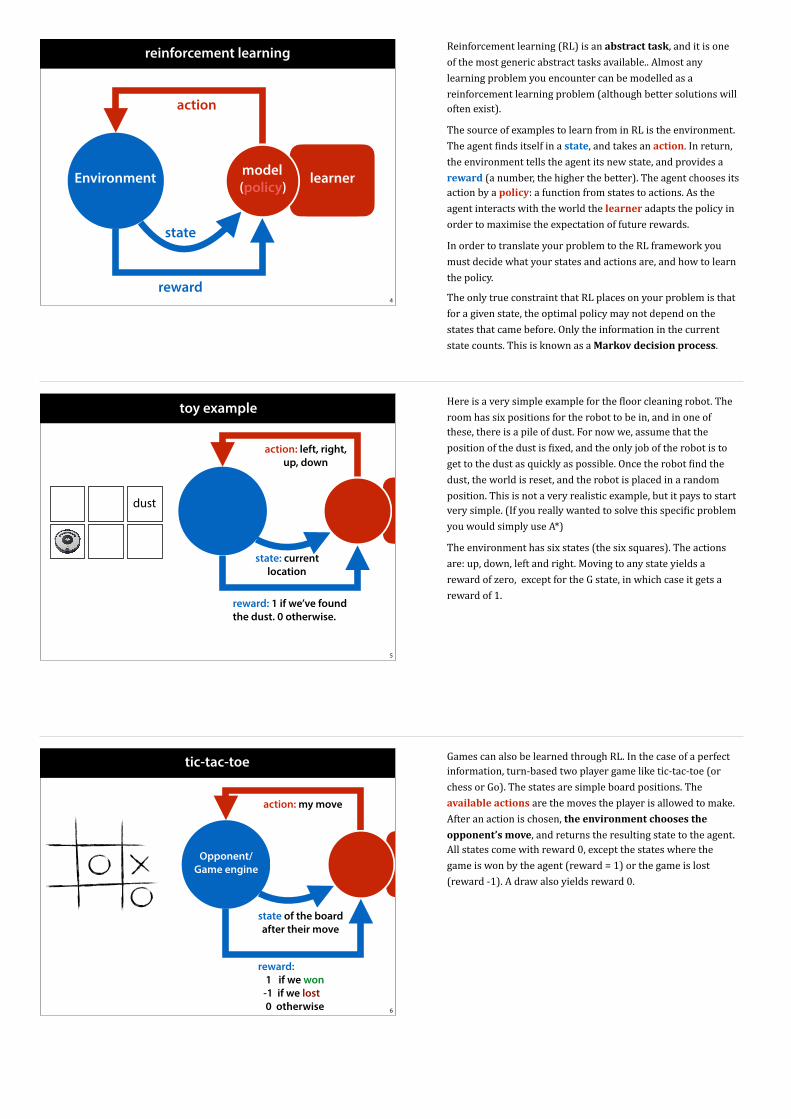
Reinforcement learning (RL) is an abstract task, and it is one of the most generic abstract tasks available.. Almost any learning problem you encounter can be modelled as a reinforcement learning problem (although better solutions will often exist).

The source of examples to learn from in RL is the environment. The agent %inds itself in a state, and takes an action. In return, the environment tells the agent its new state, and provides a reward (a number, the higher the better). The agent chooses its action by a policy: a function from states to actions. As the agent interacts with the world the learner adapts the policy in order to maximise the expectation of future rewards.

In order to translate your problem to the RL framework you must decide what your states and actions are, and how to learn the policy.

The only true constraint that RL places on your problem is that for a given state, the optimal policy may not depend on the states that came before. Only the information in the current state counts. This is known as a Markov decision process.

toy example

5

state: current location

reward: 1 if we’ve found the dust. 0 otherwise.

action: left, right, up, down

dust

Here is a very simple example for the %loor cleaning robot. The room has six positions for the robot to be in, and in one of these, there is a pile of dust. For now we, assume that the position of the dust is %ixed, and the only job of the robot is to get to the dust as quickly as possible. Once the robot %ind the dust, the world is reset, and the robot is placed in a random position. This is not a very realistic example, but it pays to start very simple. (If you really wanted to solve this speci%ic problem you would simply use A*)

The environment has six states (the six squares). The actions are: up, down, left and right. Moving to any state yields a reward of zero, except for the G state, in which case it gets a reward of 1.

tic-tac-toe

6

Opponent/ Game engine

state of the board after their move

reward: 1 if we won -1 if we lost 0 otherwise

action: my move

Games can also be learned through RL. In the case of a perfect information, turn-based two player game like tic-tac-toe (or chess or Go). The states are simple board positions. The available actions are the moves the player is allowed to make. After an action is chosen, the environment chooses the

opponent’s move, and returns the resulting state to the agent. All states come with reward 0, except the states where the game is won by the agent (reward = 1) or the game is lost (reward -1). A draw also yields reward 0.

cart pole

7

physics engine/ real world

angle of pole

reward: -1 if poll vertical 0 otherwise

left, right

image source: https://medium.com/@tuzzer/cart-pole-balancing-with-q-learning-b54c6068d947

8source: https://www.youtube.com/watch?v=VCdxqn0fcnE

Here is an example with a slightly faster rate of actions chosen: controlling a helicopter. The helicopter is %itted with a variety of sensors, telling it which way up it is, how high it is, it’s speed and so on. The combined values for all these sensors at a given moment form the state. The actions following this state are the possible speeds of the main and tail rotor. The rewards, again, are zero unless the helicopter crashes, in which case it gets a negative reward. To train the helicopter to do speci%ic tricks (like %lying upside down), we can give certain states a positive reward depending on the trick

source: https://www.youtube.com/watch?v=VCdxqn0fcnE

sparse loss

Start with imitation learning:Supervised learning, copying human action

Reward shaping:Guessing the reward for intermediate states, or states near to good states.

Auxiliary goals:Curiosity, maximum distance traveled

9

Good explanation of reward shaping: https://

www.youtube.com/watch?v=xManAGjbx2k

DeepMind Atari

10

One bene%it of RL is that a single system can be developed for many different tasks, so long as the interface between the world and the learner stays the same. Here is a famous experiment by DeepMind, the company behind AlphaGo. The environment is an Atari simulator. The state is a single image, containing everything that can be seen on the screen. The actions are the four possible movements of the joystick and the pressing of the %ire button. The reward is determined by the score shown on the screen.

The amazing thing here is that the system was not pre-programmed with any knowledge of any of the games. For several of the games the system learned play the game better than the top human performance. source: https://www.youtube.com/watch?v=V1eYniJ0Rnk

a policy network

11

state

action

posi

tion

angl

e

left

right

softmaxs s

Before we decide how to train our model, let’s decide what it is, %irst. There are many ways to represent RL models, but most of the recent breakthroughs have come from using neural networks. Our job is to map states to actions, to states to a distribution over actions. We represent the state by two numbers (the position of the cart and the angle of the pole) and we use a softmax output layer to produce a probability distribution over the two possible actions.

If we somehow %igure out the right weights, this is all we need to solve the problem: for every state, we simply feed it through the network and either choose the action with the highest probability, or sample from the outputs.

So now all we need is a way to %igure out the weights.

the three problems of RL

Non differentiable loss

Balance exploration and exploitation

Delayed reward/sparse loss

12

If your problem has any of these properties, it can pay to tackle in a reinforcement learning setting.

This can cause some confusion when the problem doesn’t

exploration vs. exploitation

in state s, take action a

13

+1

start

+100

This is a classic trade-off in online learning: exploration vs.

exploitation. Look at this scenario. Each time the agent %inds a reward it is reset to the start state.

An agent stumbling around randomly will most likely %ind the reward top right %irst. After a few resets it has a good policy to reach that states. If it exploits only the things it has learned so far, it will keep coming back for the +1 reward, never-ending the +100 reward at the end of the long tunnel. An agent that follows a more random policy will explore more and eventually %ind the bigger treasure. At %irst, however, the exploring agent does markedly worse than the exploiting agent.

There is no de%inite answer to how to optimise this tradeoff, although a few best practices exist.

credit assignment problem

14

r(s,a) =0

r(s,a) =0

r(s,a) =0

r(s,a) =0

r(s,a) =0

r(s,a) =0

r(s,a) =-1

The main problem in reinforcement learning, is that we have to decide on our immediate action, but we don’t get immediate feedback. If the pole falls over, it may be because we made a mistake 20 timesteps ago, but we only get the (negative) reward when the pole %inally tips over. Once the pole started tipping over to the right, we may have move right twenty times: these were good actions, that should be rewarded, they were just too late to save the situation.

Another example is crashing a car. If we’re learning to drive, this is a bad outcome that should carry a negative reward. However most people brake just before they crash. These are good actions that led to a bad outcome. We shouldn’t learn not to brake before a crash, we should work backward to where we went wrong (lik taking a turn at too high a speed) and apply the negative feedback to those actions.

This is what’s called the credit assignment problem, and it’s what reinforcement learning is all about.

notation

reward function: r(s, a) = 0.01 (the higher the better)

state transitions d(s, a) = s’

policy π(s) = a or p(a|s) = 0.2

15

the

envi

ronm

ent

our m

odel

s’r(s’, a)

a

π(s) = ad(s, a) = s’

Here is some basic notation for the elements of Reinforcement learning. In most cases, the agent will not have access to the reward function, or the transition function and it will have to learn them. Sometimes the agent will learn a deterministic policy, where every state is always followed by the same action. In other cases it’s better to learn a probabilistic policy where all actions are possible, but certain ones have a higher probability.

also possible

16

probabilistic state transitions

partially observablestates

G

Here are some extensions to RL that we won’t go into (too much) today.

Sometimes the state transitions are probabilistic. Consider the example of controlling a robot: the agent might tell its left wheel to spin 5 mm, but on a slippery %loor the resulting movement may be anything from 0 to 5 mm.

Another thing you may want to model is partially observable states. For example, in a poker game, there may be %ive cards on the table, but three of them might be face down.

image source: http://www.dwaynebaraka.com/blog/

2013/10/03/why-most-csr-budgets-are-wasted/

choosing the weights (aka learning)

17

state

action

posi

tion

angl

e

0.9

0.1

softmax

reward = 0

“move left”

Simple backpropagation doesn’t work, because we don’t have labeled examples that tell us which move to take for a given state. All we can do, is choose a move and observe the reward. And as mentioned, a big reward (positive or negative) is usually a response to the action chosen a while ago instead of the current action.

So how do we turn this into a way to update our weights?

random search

pick a random point m in the model space

loop:

pick a random point m’ close to m

if loss(m) < loss(m’):

m <- m’

18

Let’s start with a very simple example: random search.

“close to”

19

m

m’m

m’m

The basic random search algorithm chooses the next point by sampling uniformly among all points with some pre-chosen distance r from w. Formally: it picks from the hypersphere (or circle, in 2D) with radius r, centered on w.

random search

20

Here is random search in action. The transparent red offshoots are successors that turned out to be worse than the current point. The algorithm starts on the left, and slowly (with a bit of a detour) stumbles in the direction of the low loss region.

random search (Dec 2017)

21

policy gradient descent

22

r(s,a) =0

r(s,a) =0

r(s,a) =0

r(s,a) =0

r(s,a) =0

r(s,a) =0

r(s,a) = 1<- go

od

<- good

<- good

<- good

<- good

<- good

<- good

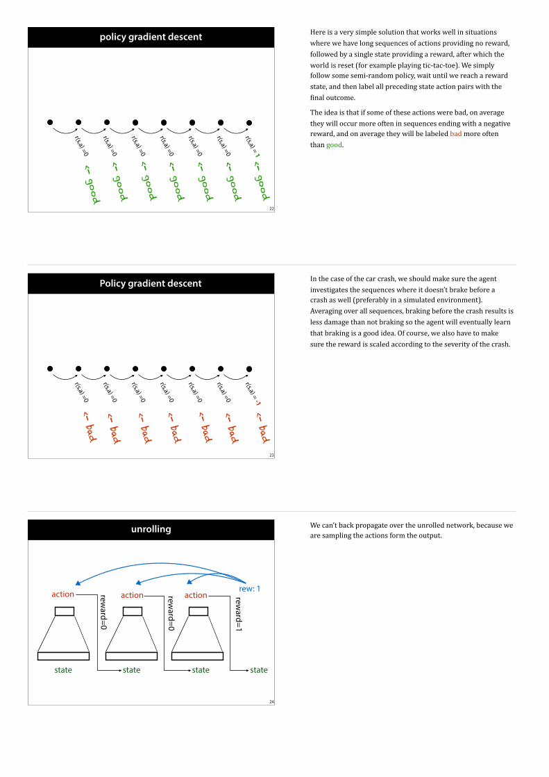
Here is a very simple solution that works well in situations where we have long sequences of actions providing no reward, followed by a single state providing a reward, after which the world is reset (for example playing tic-tac-toe). We simply follow some semi-random policy, wait until we reach a reward state, and then label all preceding state action pairs with the %inal outcome.

The idea is that if some of these actions were bad, on average they will occur more often in sequences ending with a negative reward, and on average they will be labeled bad more often than good.

Policy gradient descent

23

r(s,a) =0

r(s,a) =0

r(s,a) =0

r(s,a) =0

r(s,a) =0

r(s,a) =0

r(s,a) = -1<- bad

<- bad

<- bad

<- bad

<- bad

<- bad

<- bad

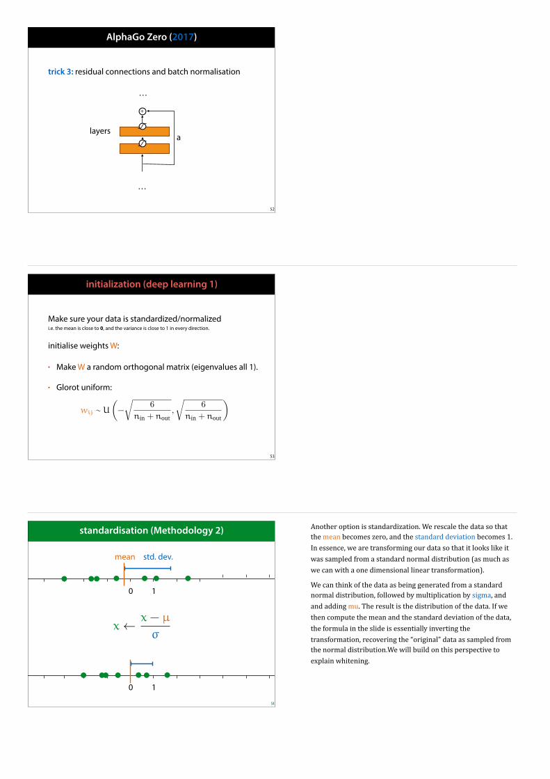
In the case of the car crash, we should make sure the agent investigates the sequences where it doesn’t brake before a crash as well (preferably in a simulated environment). Averaging over all sequences, braking before the crash results is less damage than not braking so the agent will eventually learn that braking is a good idea. Of course, we also have to make sure the reward is scaled according to the severity of the crash.

unrolling

24

state state

action

state

action

state

action reward=1

reward=0

reward=0

rew: 1

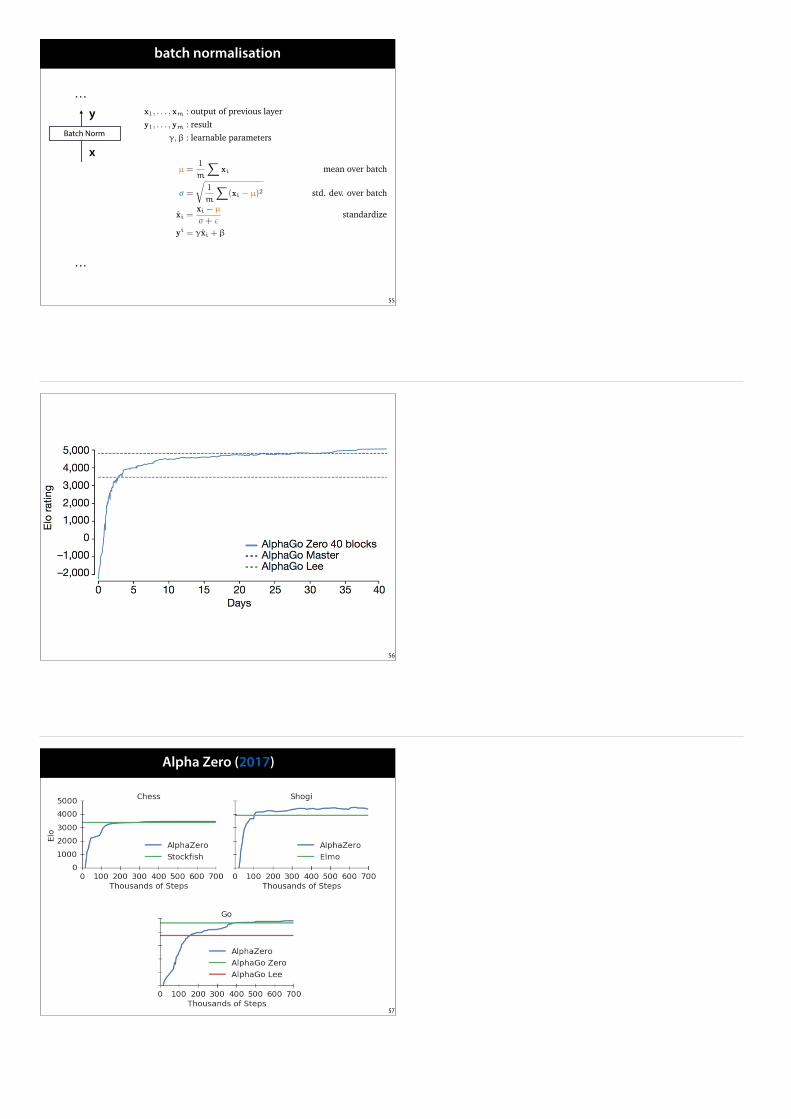
We can’t back propagate over the unrolled network, because we are sampling the actions form the output.

25image source: http://karpathy.github.io/2016/05/31/rl/

image source: http://karpathy.github.io/2016/05/31/rl/

policy gradients: the math

26

rEar(a) = rX

a

p(a)r(a)

=X

a

rp(a)r(a)

=X

a

p(a)rp(a)

p(a)r(a)

=X

a

p(a)r lnp(a)r(a) r ln(z) =1

zrz

= Ear(a)r lnp(a)<latexit sha1_base64="NilzGXAaMr2q4WPQA0ew7AzSfnA=">AAAIunicjVVdb9s2FJXbrfO8dWu2x70IM1akgxFIzpqkwAJ0TbIW29pkQewUiIyAoq9twZREkJRjmeBP2w/Z8163/zDqy9HXhurFF/ecc8l7eE26lHhcWNafnQcPP/r40SfdT3ufff74iy+f7Hw15mHEMIxwSEL23kUciBfASHiCwHvKAPkugWt3eZLg1ytg3AuDKxFTmPhoHngzDyOhU7c7nbETIJcg0zm7dRiWSJlsNwuemU+PzQLlkV/gdIvfMx2np8kVWq78QPY9zZkxhGVdreR9+MGV8r2ToHUXT01nuV1Ik3Y3z8zjfHlbyc22hY0qlmnxqHWRXu/2Sd/as9LPbAZ2HvSN/Lu43Xn0qzMNceRDIDBBnN/YFhUTiZjwMAHVcyIOFOElmsNNJGZHE+kFNBIQYGV+p7FZREwRmskhm1OPARYk1gHCzNMVTLxAujGhR6FXLcUhQD7wwXTlUZ6FfDXPAqF7g4lcp3OmHleUcs4QXXh4XdmaRD73kVg0kjz23WoSIgJs5VeTyTb1JmvMNTDs8cSEC+3MOU1ml1+FFzm+iOkCAq5kxIgqCzUAjMFMC9OQg4ioTLvRf5glPxYsgkESprnjU8SWlzAd6DqVRHU7MxIiUU25ug3tTgB3OPR9FEylQ5V0BKyFdAZ7KvWujF4qKZ3EKNc1LxO4gr4roe+UqoJnJfBMg1V0tEVn5qguHZfAcWPV6xJ6XZe6UQmNGuiqhK4ald27EnzXgNcldN1A4xIaN9BNCd00fUZ6LG6GE5mdRXqo8px4K3jNAAIl+0NV74Xp876xq5JkBmTfVqndU5jp2zYD/DihyzdXb39T8uRo+Nw6UHWGSyIoKNb+wfMTq0GZZ7vJOdbR0fBVgxMyFMy3hU7PDn6ym4VoxCjZkg4P939+0awUAyHh3bbSyavT4X59jhhumJD3avZts2HavI2ed9UqcNsEmVOt/GWT/5qh+D/YYVv1wsBWBW1TFG62KuI2RWFtoag1QZNpTV4dmtzriGSUU9A3PoO3eorP9S2FRMi+16PL5r6n7dO/ziCJ/o+I1gVRR+nzY9cfm2YwHu7Z+3vW7z/0X/6SP0Rd4xvjW2PXsI1D46XxxrgwRgbu/NH5q/N355/uj12363WXGfVBJ9d8bVS+rvgXHpwjAA==</latexit>

rEar(a) = rX

a

p(a)r(a)

=X

a

rp(a)r(a)

=X

a

p(a)rp(a)

p(a)r(a)

=X

a


zrz


rEar(a) = rX

a

p(a)r(a)

=X

a

rp(a)r(a)

=X

a

p(a)rp(a)

p(a)r(a)

=X

a


zrz


rEar(a) = rX

a

p(a)r(a)

=X

a

rp(a)r(a)

=X

a

p(a)rp(a)

p(a)r(a)

=X

a


zrz


rEar(a) = rX

a

p(a)r(a)

=X

a

rp(a)r(a)

=X

a

p(a)rp(a)

p(a)r(a)

=X

a


zrz


rEar(a) = rX

a

p(a)r(a)

=X

a

rp(a)r(a)

=X

a

p(a)rp(a)

p(a)r(a)

=X

a


zrz


rEar(a) = rX

a

p(a)r(a)

=X

a

rp(a)r(a)

=X

a

p(a)rp(a)

p(a)r(a)

=X

a


zrz


Note r is not the immediate reward but the ultimate reward at the end of the trajectory.

Q-Learning

27

A B

While policy gradient descent is a nice trick, it doesn’t really get to the heart of reinforcement learning. To understand the problem better let’s look at Q-learning, which is what was used in the Atari challenge.

The example we’ll use is the robotic hoover, also used in the %irst lecture. We will make the problem so simple that we can write out the policy explicitly: The room will have two states, the hoover can move left or right, and one of the states has dust in it. Once the hoover %inds the dust, we reset. (The robot is reset to state A, and the dust is replaced, but the robot keeps its learned experience).

what do we want to optimize?

discounted reward: r(s0, a0) + γ r(s1, a1) + γ2 r(s2, a2) + γ3 r(s3, a3) + …

with γ = 0.99or something similarly close to 1

28

If we %ix our policy, then we know for a given policy what all the future states are going to be, and what rewards we are going to get. The discounted reward is the value we will try to optimise for: we want to %ind the policy that gives us the greatest discounted reward for all states. Note that this can be an in%inite sum.

Note also that we are limiting ourselves here to deterministic policies: for a %ixed policy we always do the same thing in the same state.

If our problem is %inished after a certain state is reached (like a game of chess) the discounted reward has a %inite number of terms. If the problem can (potentially) go on forever (like the cart pole) the sum has an in%inite number of terms. In that case the discounting ensures that the sum still converges to a %inite value.

definitions

policy: π(s)

value function:Vπ(s0) = r(s0, a0) + γ r(s1, a1) + γ2 r(s2, a2) + …

Vπ(s0) = r(s0, a0) + γ Vπ(s1)

29

optimal policy:π* : the π such that for all states s, π* = argmax Vπ(s)

optimal value function:V*(s) = Vπ*(s)

π

The discounted reward we get from state s for a given policy π is called Vπ(s0), the value function. This represents the value of state s: how much we like to be in state s, given that we stick to policy π.

Using the value function, we can de%ine our optimal policy, π*. This the policy that gives us the highest value function for all states. Note that this is always possible if policy A gives us the maximal value in state s but not in state q, and policy B gives us the maximal value in state q but not in state s, we can de%ine a new policy that follows A in state s and B in state q.

We can then de%ine V*(s), which is just the value function for the optimal policy.

definitions

π*(s) = argmax [ “discounted reward of V*” ]

π*(s) = argmax [ r(s, a) + γ V*(d(s, a))]

30

Q*(s, a) = r(s, a) + γ V*(d(s, a))

π*(s) = argmax Q*(s, a) a

V*(s) = max Q*(s, a)a

a

a

Using V* we can rewrite π* as a recursive de%inition. The optimal policy is the one that chooses the action which maximises the future, assuming that we follow the optimal policy. We %ill in the optimal value function to get rid of the in%inite sum. We’ve now de%ined the optimal policy in a way that depends on what the optimal policy is. While this doesn’t allow us to compute π*, it does de4ine it. If someone gives us a policy, we can recognise it by checking if this equality holds.

To make this easier, we take the part inside the argmax and call it Q(s, a). We then rewrite the de%initions of the optimal policy and the optimal value function in terms of Q(s,a).

How has this helped us? Q(s,a) is a function from state-action pairs to a number expressing how good that particular pair is. If we were given Q, we could automatically compute the optimal policy, and the optimal value function. And it turns out, that in many problems it’s much easier to learn the Q-function, than it is to learn the policy directly.

making the definition of Q* recursive

Q*(s, a) = r(s, a) + γ V*(d(s, a))

Q*(s, a) = r(s, a) + γ max Q*(d(s, a), a’)

31

a’

In order to see how the Q function can be learned we rewrite it. Earlier, we rewrote the V functions in terms of the Q function, now we plug that de%inition back into the Q function. We now get a recursive de%inition of Q.

Again, this may be a little dif%icult to wrap your head around. If so think of it this way: If we were given a random Q-function, how could we tell whether it was optimal? We don’t know π* or V* so we can’t use the original de%initions. But this equality must hold true! If we loop over all possible states and actions, and plug them into this equality, we must get the same number on both sides. Let’s try it for a simple example.

Is my Q-function optimal?

32

s a r(s,a) Q(s,a)

A L 0 1

A R 1 2

B L 0 1

B R 0 -1

A B

Q(s, a) = r(s, a) + γ max Q(d(s, a), a’)a’

r(A, R) = 1, all others 0

?

This is the two-state hoover problem again. We have states A and B, and actions left and right. The agent only gets a reward when moving from A to B. On the bottom left we see some random policy, generated by assigning random numbers to each state action pair. Did we get lucky and stumble on the optimal policy? Try it for yourself and see. (take γ = 0.9)

solving recurrent equations by iteration

33

x = x2 - 2

x= 0 :

0 ! 02 - 2 = -2

x= -2 :

-2 ! -22 - 2 = 2

x= 2 :

2 ! 22 - 2 = 2<latexit sha1_base64="qcB5mvPQdH1a6aSKB9hmNmFivQ4=">AAAIEHicfVVdb9s2FJW7rm69dk3Xx70QNVYUgxNIypqkAwy0cbIW29pkQZwUiLyAoq9lwdQHSMqWSuhP7H/sfW/DXvcP9m9GWbKhr40vur7nnGvewwvSDqnLha7/07nz2d3P73XvP+h98fDRl493nnx1xYOIERiTgAbso405UNeHsXAFhY8hA+zZFK7txSjDr5fAuBv4lyIJYeJhx3dnLsFCpW53fo/R8yGKfzXRLjKRZfWsBZFxip5n3yHSv0+zpK5+M9eZC8xYsEJ6QR+i3RbNrpmLFFZR7ZpbWYuqENU0NcntTl/f09cLNQOjCPpasc5vn9z7yZoGJPLAF4Rizm8MPRQTiZlwCYW0Z0UcQkwW2IGbSMyOJtL1w0iAT1L0jcJmEUUiQJl1aOoyIIImKsCEuaoCInPMMBHK4F61FAcfe8AH06Ub8jzkSycPBFanM5Hx+vTSRxWldBgO5y6JK1uT2OMeFvNGkieeXU1CRIEtvWoy26baZI0ZAyMuz0w4V86chdlE8MvgvMDnSTgHn6cyYjQtCxUAjMFMCdchBxGFct2NGsMFHwoWwSAL17nhCWaLC5gOVJ1KorqdGQ2wqKZs1YZyx4cVCTwP+1Npham0BMRCWoO9dO1dGb1IpbQyo2wbXWRwBf1QQj+kaRU8LYGnCqyi4y06Q+O69KoEXjX+9bqEXteldlRCowa6LKHLRmV7VYJXDTguoXEDTUpo0kA/ldBPTZ+xGosbcyLzs1gfqjyj7hLeMgA/lX0zrffC1HnfGFVJNgOyb6Rru6cwU3dYDnhJRpfvLt//nMrRkflSP0jrDJtGsKHo+wcvR3qD4uS7KTj60ZF53OAEDPvOttDJ6cEbo1kojFhIt6TDw/0fXjUrJUBpsNpWGh2fmPv1OWKkYULRK+obqGGa00YvumoV2G2C3KlW/qLJf8tw8h/soK36xsBWRdim2LjZqkjaFBtrN4paE2E2reoVscLsXsc0p5yAuvEZvFdTfKZuKSwC9q0aXeZ4rrJPfa1BFv0fEccboop62fNj1B+bZnBl7hn7e/ov3/Vf/1g8RPe1r7Vn2gvN0A6119o77Vwba6TztPOqc9wZdX/r/tH9s/tXTr3TKTRPtcrq/v0vwADeiQ==</latexit>

x = x2 - 2

x= 0 :

0 ! 02 - 2 = -2

x= -2 :

-2 ! -22 - 2 = 2

x= 2 :


x = x2 - 2

x= 0 :

0 ! 02 - 2 = -2

x= -2 :

-2 ! -22 - 2 = 2

x= 2 :


x = x2 - 2

x= 0 :

0 ! 02 - 2 = -2

x= -2 :

-2 ! -22 - 2 = 2

x= 2 :


Of course, random sampling of policy functions is not an ef%icient search method. How do we get from a recursive de%inition to the value that satis%ies that de%inition? Here is a simple example from a single number: de%ine x as the value for which x = x2 - 2 holds. This is analogous to the de%inition above: we have one x on the left and a function of x on the right.

Of course, we all learned in high school how to solve this by rewriting, but we can also solve it by iteration. We replace the equals sign by an arrow and write: x <- x2 - 2. We start with some randomly chosen value of x, compute x2 - 2, and replace x by the new value. We iterate this and we end up with a functions for which the de%inition holds. Try it for yourself (start with x = 0)

Note that in this example in%inity also counts as a solution, so if you pick the wrong starting state you may end up with larger and larger numbers. For other functions, there may be stable states that jump back from one point to another, or even chaotic states (see https://en.wikipedia.org/wiki/Logistic_map for more information if you’re interested, but this is not exam material).

Q-Learning

init Q(s, a) = 0 for all s and a

loop: • in state s, take action a

• arrive in s’ • receive reward r

• update Q(s, a) <- r + γ max Q(s’, a’)

34

a’

This gives us the Q-learning algorithm shown here.

Note that the algorithm does not tell you how to choose the action. It may be tempting to use your current policy to choose the action, but that may lead you repeat early successes with out learning much about the world.

NB:While we are learning a deterministic policy here (the Q function), the function that decides which actions to take can be anything, and should contain some randomness.

35

A

B C

D F

E

s a Q(s,a)A U 0A R 0B U 0B R 0C U 0C R 0D U 0D R 0E U 0

Q(s,a)000000000

U

Q(s,a)000000000

R R

Q(s,a)000001000

Q(s, a) <- r + γ max Q(s’, a’)

Q(s,a)000001000

U R R

*reset*Q(s,a)

0000

0.91000

Q(s,a)0000

0.91000

a’

A B C E A B C E

To see how Q learning operates, imagine setting a robot in the bottom-left square (A) in the %igure shown and letting it explore. The robot chooses the actions up, right, right and when it reaches the goal state (E) it gets reset to the start state. It gets +1 immediate reward for entering the goal state and 0 reward for any other action.

What we see is that the Q function stays 0 for all values until the robot enters the goal state. At that point Q(C, R) west updated to value one. In the next run, Q(B, R) gets updated to 0.9. In the next run after, Q(A, U) is updated to 0.9 * 0.9. This is how Q-learning updates. In every run of the algorithm the immediate rewards from the previous runs are propagated to neighbouring states.

Q-Learning

Which actions should we take?

epsilon-greedy: follow current pollicy, expect with probability epsilon, take a random actionDecay epsilon as learning progresses

36

Deep Q-learning

update Q(s, a) <- r + γ max Q(s’, a’)

37

a’

s

a

break

38source: https://warandpeas.com/2016/10/09/robot/

AlphaGO

39

source: https://www.youtube.com/watch?v=8tq1C8spV_g

In 2016 AlphaGo, a Go playing computer developed by the company DeepMind beat the world champion Lee Sedol. Many AI researchers were convinced that this AI breakthrough was at least decades away.

image source: http://gadgets.ndtv.com/science/news/lee-

sedol-scores-surprise-victory-over-googles-alphago-in-

game-4-813248

The game of Go

41

First, some intuition about how Go works. The rules are very simple: players (black and white) move, one after the other, placing stones on a 19 by 19 grid. The aim of the game is to have as many stones on the board, when no more stones can be placed. The only way to remove stones is to encircle your opponent. Why is Go so dif%icult and what has AlphaGo done to %inally solve these issues?

claims from the media

AlphaGo is an important move towards general purpose AI.

AlphaGo thinks and learns in a human way.

AlphaGo mimics the human brain.

Go has more possible positions than there are atoms in the universe. That’s why it’s difficult.

What makes Go difficult is the high branching factor.

42

When the win against Lee Sedol was publicised, many claims were made in the media, some by DeepMind themselves. Here are some of them. All of these are dubious for various reasons

From top to bottom:

• AlphaGO is very much purpose-built for Go. It’s not an architecture that can be translated 1-on-1 to any other games, and Go has some features that are exploited in a very speci%ic way. However, DeepMind hasher projects that are impressive milestones toward general purpose AI. It’s also true that projects like Deep Blue (the chess computer that beat Kasparov) were %illed with hand-coded chess knowledge, written with the help of experts. This is not true for AlphaGo: the rules of Go were hardcoded into it, and it learned everything else by simply observing existing matches, and playing against itself

• AlphaGo learns. It’s thinking is probably more human than Deep Blue’s, but we don’t understand human thinking well enough to make this claim.

• AlphaGo uses convolutional neural networks, which very loosely inspired by brain architecture.

minimax

43

The minimax algorithm is mostly useless when it comes to Go. For each node in the tree there are up to 361 children, compared to about 30 for chess. This means almost 17 billion terminal nodes if we just search two turns deep. And as we discussed, you need to search very deep to %ind the nodes that show clear rewards.

image source: By Nuno Nogueira (Nmnogueira) - http://

en.wikipedia.org/wiki/Image:Minimax.svg, created in Inkscape by author, CC BY-SA 2.5, https://commons.wikimedia.org/w/

index.php?curid=2276653

rollouts

44

This simple principle was an early success in playing Go: we simply choose random moves from some fast policy, and play a few full games for each immediate successor. We then average the rewards we got over these as a value for the successor states, and choose the action that lead to the highest values. The rollout policy should ideally give good moves high probability, but also be very fast to compute.

monte-carlo tree search (MCTS)

45

Monte Carlo Tree Search (MCTS) is a simple, but effective algorithm, combining rollouts with an incomplete tree search. We start the search with an unexpanded root node labeled 0/0 (this value represents the probability of winning from the given state). We then iterate the following algorithm

• Selection: select unexpanded node. At %irst, this will be the root node. But once the tree is further expanded we perform a random walk from the root down to one of the leaves.

• Expansion: Once we hit a leaf (an unexpanded node), we expand it and give its children the value 0/0.

• Simulation: From each expanded child we do a rollout.

• Back propagation (nothing to do with the backpropagation we know from NNs): If we win the rollout let v = 1 otherwise v = 0. For the new child and everyone of its parents update the value. If the old value was a/b, the new value is a+v / b+1. The value is the proportion of simulated games crossing that state that we’ve won.

The random walk performed in the selection phase should favour nodes with a high value, but also explore the nodes with

AlphaGo (2016)

46

the functions that AlphaGo learns are convolutional networks. One type is a policy network (from states to moves) and one is a value network (from states to a numeric value).

Here are the networks it learns

SL: policy network: from a database of games (like ALVINN, watching human drivers)

RL: policy network, start with SL, but re%ine with reinforcement learning (policy gradient descent)

slow policy network (with softmax layer on top )

fast policy network with (with linear activations)

V: value network learned from observing older versions of itself playing games. Once the game is %inished and the outcome of the game (eg. “black wins”) is used as the label for all the states observed in the game.

The value network predicts the winner form the current board state.

putting it all together

start with imitation learning.

improve by playing against previous iterations and selfupdate weights by policy gradients

Boost network performance by MCTS

47

The networks are trained by reinforcement learning using policy gradient descent.

During actual play, AlphaGO uses an MCTS algorithm. The value on each node (as in basic MCTS) represents the probability that black will win from that state.

- When it comes to rollouts, use the slow policy network to do a rollout for T steps, then %inish with the fast policy

- The value v of the newly opened state is the average of the value (computed with the the value network) after T steps, and the win/lose value at the end of the rollout. (image c)

- Backup as with standard MCTS: each node’s value becomes the probability of a win from that state. Precisely the value of node n becomes the sum of the values of all simulations crossing node n, divided by the total number of simulations crossing node n. A simulation is counted as a full game simulated from the root node down to a terminal (win/loss) node. (image(d))

AlphaGo Zero (2017)

Learns from scratch, no imitation learning, reward shaping etc.Also applicable to Chess, Shogi…

Uses three tricks to simplify/improve AlphaGo

1. Combine policy and value nets

2. View MCTS as a policy improvement operator

3. Add residual connections, batch normalization

48

AlphaGo Zero (2017)

trick 1: combine policy and value nets.

49

AlphaGo Zero (2017)

trick 2: view MCTS as a policy improvement operator.

50

image source: Mastering the game of Go without human

knowledge, David Silver, Julian Schrittwieser, Karen Simonyan et al.

AlphaGo Zero (2017)

trick 2: view MCTS as a policy improvement operator.

51

image source: Mastering the game of Go without human knowledge, David Silver, Julian Schrittwieser, Karen Simonyan et

al.

AlphaGo Zero (2017)

trick 3: residual connections and batch normalisation

52

+

layersa

…

…

initialization (deep learning 1)

Make sure your data is standardized/normalized i.e. the mean is close to 0, and the variance is close to 1 in every direction.

initialise weights W:

• Make W a random orthogonal matrix (eigenvalues all 1).

• Glorot uniform:

53

wij ⇠ U

✓-

r6

nin + nout,

r6

nin + nout

◆

<latexit sha1_base64="O3jviuWNpP291jJzAXNpBSmkLGY=">AAAINHicjVXLbttGFKXcJkqUR512mQ0RIUDaKAYpN7a7CJD40WTRxK5h2QFMQRiOLilWw0dnhpKYwfxOP6H/UiC7ott+Q4aipJActghXV/ecc3nn3KGum5CAccv6q7X11dc3brZv3e7cuXvv/jfbD769ZHFKMQxwTGL63kUMSBDBgAecwPuEAgpdAlfu9CjHr2ZAWRBHFzxLYBgiPwq8ACOuUqPtmRNjMR+J4DcpTYcFoTlwCHj8yTOH/U65cDyKsNiTIho5HBZcBJF8aq5/xCmXUvbML+c6NPAn/PvRdtfasZaPqQf2Kugaq+ds9ODmH844xmkIEccEMXZtWwkfCkR5gAnIjpMySBCeIh+uU+4dDNXbk5RDhKX5WGFeSkwem7kH5jiggDnJVIAwDVQFE0+Qap4rpzrVUgwiFALrjWdBwoqQzfwi4EjZPBSL5RjkvYpS+BQlkwAvKq0JFLIQ8YmWZFnoVpOQEqCzsJrM21RN1pgLoDhguQlnypnTJB8tu4jPVvgkSyYQMSlSSmRZqACgFDwlXIYMeJqI5WnUfZqyF5ym0MvDZe7FMaLTcxj3VJ1KotqOR2LEqylXHUO5E8Ecx2GIorFwEimKe+H0duTSuzJ6LoVwcqNc1zzP4Qr6roS+k7IKnpTAEwVW0cEG9cxBXXpZAi+1t16V0Ku61E1LaKqhsxI60yq78xI81+BFCV1oaFZCMw39UEI/6D4jdS2u+0NRzGI5VHFKghm8pgCRFN2+rJ+Fqnlf21VJfgdE15ZLu8fgqT+jAgiznC7eXLz9RYqjg/5za0/WGS5JYU2xdveeH1kaxS+6WXGsg4P+ocaJKYr8TaHjk71Xtl4oSWlCNqT9/d2ff9IrZUBIPN9UOjo87u/WD6YcqTZl79uWVb9tFGtWrRwxu7apWes30VevaRS4TYLCz0b+VOe/pij7D3bcVH1tc6MiaVKsPW9UZE2K9QDWiqokarDp8zg2mtrJk/xDmGLVY74yECnqHoNaJhTeqg/kVP0BIh7TH9RXQf1Q7S61XHynl0f/R0SLNVFFnY7abHZ9j+nBZX/HtnbsX3/svjxc7bhbxkPjkfHEsI1946XxxjgzBgY2Pra2Wndad9t/tj+2/27/U1C3WivNd0blaf/7CT/7/6Y=</latexit><latexit sha1_base64="O3jviuWNpP291jJzAXNpBSmkLGY=">AAAINHicjVXLbttGFKXcJkqUR512mQ0RIUDaKAYpN7a7CJD40WTRxK5h2QFMQRiOLilWw0dnhpKYwfxOP6H/UiC7ott+Q4aipJActghXV/ecc3nn3KGum5CAccv6q7X11dc3brZv3e7cuXvv/jfbD769ZHFKMQxwTGL63kUMSBDBgAecwPuEAgpdAlfu9CjHr2ZAWRBHFzxLYBgiPwq8ACOuUqPtmRNjMR+J4DcpTYcFoTlwCHj8yTOH/U65cDyKsNiTIho5HBZcBJF8aq5/xCmXUvbML+c6NPAn/PvRdtfasZaPqQf2Kugaq+ds9ODmH844xmkIEccEMXZtWwkfCkR5gAnIjpMySBCeIh+uU+4dDNXbk5RDhKX5WGFeSkwem7kH5jiggDnJVIAwDVQFE0+Qap4rpzrVUgwiFALrjWdBwoqQzfwi4EjZPBSL5RjkvYpS+BQlkwAvKq0JFLIQ8YmWZFnoVpOQEqCzsJrM21RN1pgLoDhguQlnypnTJB8tu4jPVvgkSyYQMSlSSmRZqACgFDwlXIYMeJqI5WnUfZqyF5ym0MvDZe7FMaLTcxj3VJ1KotqOR2LEqylXHUO5E8Ecx2GIorFwEimKe+H0duTSuzJ6LoVwcqNc1zzP4Qr6roS+k7IKnpTAEwVW0cEG9cxBXXpZAi+1t16V0Ku61E1LaKqhsxI60yq78xI81+BFCV1oaFZCMw39UEI/6D4jdS2u+0NRzGI5VHFKghm8pgCRFN2+rJ+Fqnlf21VJfgdE15ZLu8fgqT+jAgiznC7eXLz9RYqjg/5za0/WGS5JYU2xdveeH1kaxS+6WXGsg4P+ocaJKYr8TaHjk71Xtl4oSWlCNqT9/d2ff9IrZUBIPN9UOjo87u/WD6YcqTZl79uWVb9tFGtWrRwxu7apWes30VevaRS4TYLCz0b+VOe/pij7D3bcVH1tc6MiaVKsPW9UZE2K9QDWiqokarDp8zg2mtrJk/xDmGLVY74yECnqHoNaJhTeqg/kVP0BIh7TH9RXQf1Q7S61XHynl0f/R0SLNVFFnY7abHZ9j+nBZX/HtnbsX3/svjxc7bhbxkPjkfHEsI1946XxxjgzBgY2Pra2Wndad9t/tj+2/27/U1C3WivNd0blaf/7CT/7/6Y=</latexit><latexit sha1_base64="O3jviuWNpP291jJzAXNpBSmkLGY=">AAAINHicjVXLbttGFKXcJkqUR512mQ0RIUDaKAYpN7a7CJD40WTRxK5h2QFMQRiOLilWw0dnhpKYwfxOP6H/UiC7ott+Q4aipJActghXV/ecc3nn3KGum5CAccv6q7X11dc3brZv3e7cuXvv/jfbD769ZHFKMQxwTGL63kUMSBDBgAecwPuEAgpdAlfu9CjHr2ZAWRBHFzxLYBgiPwq8ACOuUqPtmRNjMR+J4DcpTYcFoTlwCHj8yTOH/U65cDyKsNiTIho5HBZcBJF8aq5/xCmXUvbML+c6NPAn/PvRdtfasZaPqQf2Kugaq+ds9ODmH844xmkIEccEMXZtWwkfCkR5gAnIjpMySBCeIh+uU+4dDNXbk5RDhKX5WGFeSkwem7kH5jiggDnJVIAwDVQFE0+Qap4rpzrVUgwiFALrjWdBwoqQzfwi4EjZPBSL5RjkvYpS+BQlkwAvKq0JFLIQ8YmWZFnoVpOQEqCzsJrM21RN1pgLoDhguQlnypnTJB8tu4jPVvgkSyYQMSlSSmRZqACgFDwlXIYMeJqI5WnUfZqyF5ym0MvDZe7FMaLTcxj3VJ1KotqOR2LEqylXHUO5E8Ecx2GIorFwEimKe+H0duTSuzJ6LoVwcqNc1zzP4Qr6roS+k7IKnpTAEwVW0cEG9cxBXXpZAi+1t16V0Ku61E1LaKqhsxI60yq78xI81+BFCV1oaFZCMw39UEI/6D4jdS2u+0NRzGI5VHFKghm8pgCRFN2+rJ+Fqnlf21VJfgdE15ZLu8fgqT+jAgiznC7eXLz9RYqjg/5za0/WGS5JYU2xdveeH1kaxS+6WXGsg4P+ocaJKYr8TaHjk71Xtl4oSWlCNqT9/d2ff9IrZUBIPN9UOjo87u/WD6YcqTZl79uWVb9tFGtWrRwxu7apWes30VevaRS4TYLCz0b+VOe/pij7D3bcVH1tc6MiaVKsPW9UZE2K9QDWiqokarDp8zg2mtrJk/xDmGLVY74yECnqHoNaJhTeqg/kVP0BIh7TH9RXQf1Q7S61XHynl0f/R0SLNVFFnY7abHZ9j+nBZX/HtnbsX3/svjxc7bhbxkPjkfHEsI1946XxxjgzBgY2Pra2Wndad9t/tj+2/27/U1C3WivNd0blaf/7CT/7/6Y=</latexit><latexit sha1_base64="O3jviuWNpP291jJzAXNpBSmkLGY=">AAAINHicjVXLbttGFKXcJkqUR512mQ0RIUDaKAYpN7a7CJD40WTRxK5h2QFMQRiOLilWw0dnhpKYwfxOP6H/UiC7ott+Q4aipJActghXV/ecc3nn3KGum5CAccv6q7X11dc3brZv3e7cuXvv/jfbD769ZHFKMQxwTGL63kUMSBDBgAecwPuEAgpdAlfu9CjHr2ZAWRBHFzxLYBgiPwq8ACOuUqPtmRNjMR+J4DcpTYcFoTlwCHj8yTOH/U65cDyKsNiTIho5HBZcBJF8aq5/xCmXUvbML+c6NPAn/PvRdtfasZaPqQf2Kugaq+ds9ODmH844xmkIEccEMXZtWwkfCkR5gAnIjpMySBCeIh+uU+4dDNXbk5RDhKX5WGFeSkwem7kH5jiggDnJVIAwDVQFE0+Qap4rpzrVUgwiFALrjWdBwoqQzfwi4EjZPBSL5RjkvYpS+BQlkwAvKq0JFLIQ8YmWZFnoVpOQEqCzsJrM21RN1pgLoDhguQlnypnTJB8tu4jPVvgkSyYQMSlSSmRZqACgFDwlXIYMeJqI5WnUfZqyF5ym0MvDZe7FMaLTcxj3VJ1KotqOR2LEqylXHUO5E8Ecx2GIorFwEimKe+H0duTSuzJ6LoVwcqNc1zzP4Qr6roS+k7IKnpTAEwVW0cEG9cxBXXpZAi+1t16V0Ku61E1LaKqhsxI60yq78xI81+BFCV1oaFZCMw39UEI/6D4jdS2u+0NRzGI5VHFKghm8pgCRFN2+rJ+Fqnlf21VJfgdE15ZLu8fgqT+jAgiznC7eXLz9RYqjg/5za0/WGS5JYU2xdveeH1kaxS+6WXGsg4P+ocaJKYr8TaHjk71Xtl4oSWlCNqT9/d2ff9IrZUBIPN9UOjo87u/WD6YcqTZl79uWVb9tFGtWrRwxu7apWes30VevaRS4TYLCz0b+VOe/pij7D3bcVH1tc6MiaVKsPW9UZE2K9QDWiqokarDp8zg2mtrJk/xDmGLVY74yECnqHoNaJhTeqg/kVP0BIh7TH9RXQf1Q7S61XHynl0f/R0SLNVFFnY7abHZ9j+nBZX/HtnbsX3/svjxc7bhbxkPjkfHEsI1946XxxjgzBgY2Pra2Wndad9t/tj+2/27/U1C3WivNd0blaf/7CT/7/6Y=</latexit>

standardisation (Methodology 2)

54

0 1

std. dev.mean

0 1

x x- µ

�<latexit sha1_base64="8j9BeoJt9JTSHyQ9yl+WPZDB8Bc=">AAAGlXicdZRLb9NAEIBdoKEECi1ckLhYREgIhcgOtIRDUaGhrRBtQtU0leKoWm/GjhW/tLtO4q72r/BruMKdf8M6cSs/wl4ynm9mNK+MGboOZZr2d+3O3XvrlfsbD6oPH20+frK1/fSCBhHB0MOBG5BLE1FwHR96zGEuXIYEkGe60DcnBwnvT4FQJ/DPWRzC0EO271gORkyqrrZaho35XKiGCxZDhAQz1bAIwjzVv1WNQH54kRDcMKVEHdtDQqhXWzWtoS2eWhb0VKgp6eteba8fGqMARx74DLuI0oGuhWzIEWEOdkFUjYhCiPAE2TCImNUacscPIwY+FuoryazIVVmgJlWoI4cAZm4sBYSJIyOoeIxk3kzWWs2HouAjD2h9NHVCuhTp1F4KDMlGDfl80UixmfPkNkHh2MHzXGocedRDbFxS0tgz80qIXCBTL69M0pRJFiznQLBDkyZ0ZWc6YTIceh50Uz6OwzH4VPCIuCLrKAEQApZ0XIgUWBTyRTVyIyZ0j5EI6om40O21EZmcwagu4+QU+XQsN0BMyGb4MMOB5yF/xI1QLgCDOeNGvSEWrcrSM8Hllsi+mKZ6luAcPc3QU1GM3LulltqTNAcvMvCiFLifof2iqxllaFSi0wydliKbswyelfA8Q+clGmdoXKLXGXpdbiWSgx40h3zZ7sWYeMd1pnBEAHzBa01RrIXICQ70vEsyVV7TxaLdI7DkgVgCL07M+fH5yXfBD1rNHW1XFC1MN4IbE+3d7s6BVjKxl9mkNlqr1fxSsgkI8u3bQO2vu591rTh9gkuppxmqNV0tlWqvMk9zWelgrnJY1rfSflK2PyIo/o91sCr6Tdk3HoWKJ2GyABN5TMPk+CF3OaM2yLNI4EQuRkf+lRELyBu5DcT2HFmb/DXqiVSVl1cv3tmy0Gs2Pja0H+9r+9/SE7yhvFBeKq8VXfmg7CvHSlfpKVj5qfxSfit/Ks8rnyrtyuHS9M5a6vNMyb1K5x+RzV2Z</latexit><latexit sha1_base64="8j9BeoJt9JTSHyQ9yl+WPZDB8Bc=">AAAGlXicdZRLb9NAEIBdoKEECi1ckLhYREgIhcgOtIRDUaGhrRBtQtU0leKoWm/GjhW/tLtO4q72r/BruMKdf8M6cSs/wl4ynm9mNK+MGboOZZr2d+3O3XvrlfsbD6oPH20+frK1/fSCBhHB0MOBG5BLE1FwHR96zGEuXIYEkGe60DcnBwnvT4FQJ/DPWRzC0EO271gORkyqrrZaho35XKiGCxZDhAQz1bAIwjzVv1WNQH54kRDcMKVEHdtDQqhXWzWtoS2eWhb0VKgp6eteba8fGqMARx74DLuI0oGuhWzIEWEOdkFUjYhCiPAE2TCImNUacscPIwY+FuoryazIVVmgJlWoI4cAZm4sBYSJIyOoeIxk3kzWWs2HouAjD2h9NHVCuhTp1F4KDMlGDfl80UixmfPkNkHh2MHzXGocedRDbFxS0tgz80qIXCBTL69M0pRJFiznQLBDkyZ0ZWc6YTIceh50Uz6OwzH4VPCIuCLrKAEQApZ0XIgUWBTyRTVyIyZ0j5EI6om40O21EZmcwagu4+QU+XQsN0BMyGb4MMOB5yF/xI1QLgCDOeNGvSEWrcrSM8Hllsi+mKZ6luAcPc3QU1GM3LulltqTNAcvMvCiFLifof2iqxllaFSi0wydliKbswyelfA8Q+clGmdoXKLXGXpdbiWSgx40h3zZ7sWYeMd1pnBEAHzBa01RrIXICQ70vEsyVV7TxaLdI7DkgVgCL07M+fH5yXfBD1rNHW1XFC1MN4IbE+3d7s6BVjKxl9mkNlqr1fxSsgkI8u3bQO2vu591rTh9gkuppxmqNV0tlWqvMk9zWelgrnJY1rfSflK2PyIo/o91sCr6Tdk3HoWKJ2GyABN5TMPk+CF3OaM2yLNI4EQuRkf+lRELyBu5DcT2HFmb/DXqiVSVl1cv3tmy0Gs2Pja0H+9r+9/SE7yhvFBeKq8VXfmg7CvHSlfpKVj5qfxSfit/Ks8rnyrtyuHS9M5a6vNMyb1K5x+RzV2Z</latexit><latexit sha1_base64="8j9BeoJt9JTSHyQ9yl+WPZDB8Bc=">AAAGlXicdZRLb9NAEIBdoKEECi1ckLhYREgIhcgOtIRDUaGhrRBtQtU0leKoWm/GjhW/tLtO4q72r/BruMKdf8M6cSs/wl4ynm9mNK+MGboOZZr2d+3O3XvrlfsbD6oPH20+frK1/fSCBhHB0MOBG5BLE1FwHR96zGEuXIYEkGe60DcnBwnvT4FQJ/DPWRzC0EO271gORkyqrrZaho35XKiGCxZDhAQz1bAIwjzVv1WNQH54kRDcMKVEHdtDQqhXWzWtoS2eWhb0VKgp6eteba8fGqMARx74DLuI0oGuhWzIEWEOdkFUjYhCiPAE2TCImNUacscPIwY+FuoryazIVVmgJlWoI4cAZm4sBYSJIyOoeIxk3kzWWs2HouAjD2h9NHVCuhTp1F4KDMlGDfl80UixmfPkNkHh2MHzXGocedRDbFxS0tgz80qIXCBTL69M0pRJFiznQLBDkyZ0ZWc6YTIceh50Uz6OwzH4VPCIuCLrKAEQApZ0XIgUWBTyRTVyIyZ0j5EI6om40O21EZmcwagu4+QU+XQsN0BMyGb4MMOB5yF/xI1QLgCDOeNGvSEWrcrSM8Hllsi+mKZ6luAcPc3QU1GM3LulltqTNAcvMvCiFLifof2iqxllaFSi0wydliKbswyelfA8Q+clGmdoXKLXGXpdbiWSgx40h3zZ7sWYeMd1pnBEAHzBa01RrIXICQ70vEsyVV7TxaLdI7DkgVgCL07M+fH5yXfBD1rNHW1XFC1MN4IbE+3d7s6BVjKxl9mkNlqr1fxSsgkI8u3bQO2vu591rTh9gkuppxmqNV0tlWqvMk9zWelgrnJY1rfSflK2PyIo/o91sCr6Tdk3HoWKJ2GyABN5TMPk+CF3OaM2yLNI4EQuRkf+lRELyBu5DcT2HFmb/DXqiVSVl1cv3tmy0Gs2Pja0H+9r+9/SE7yhvFBeKq8VXfmg7CvHSlfpKVj5qfxSfit/Ks8rnyrtyuHS9M5a6vNMyb1K5x+RzV2Z</latexit>

Another option is standardization. We rescale the data so that the mean becomes zero, and the standard deviation becomes 1. In essence, we are transforming our data so that it looks like it was sampled from a standard normal distribution (as much as we can with a one dimensional linear transformation).

We can think of the data as being generated from a standard normal distribution, followed by multiplication by sigma, and and adding mu. The result is the distribution of the data. If we then compute the mean and the standard deviation of the data, the formula in the slide is essentially inverting the transformation, recovering the “original” data as sampled from the normal distribution.We will build on this perspective to explain whitening.

batch normalisation

55

+

x

…

Batch Norm

…

y x1, . . . , xm : output of previous layery1, . . . , ym : result

�,� : learnable parameters

µ =1

m

Xxi mean over batch

� =

r1

m

X(xi - µ)2 std. dev. over batch

x̂i =xi - µ

�+ ✏standardize

yi = �x̂i + �<latexit sha1_base64="VHKEgWifsQbU5zuX+c/79NOWVGM=">AAAJA3icfVXdbuNEFHazUEJgYctecjMiolrYbGSn9AekSsu2ZVfAbkvVtCvV2WhsnyRWxj/MjNO4o7nkOXgA7hC3PAhvw7GdRHYcsCL5ZL6fOXPmeMaJmS+kaf6z1Xjw3vvbHzQ/bH308cNPPn2089m1iBLuQt+NWMTfOlQA80PoS18yeBtzoIHD4MaZnmT4zQy48KPwSqYxDAI6Dv2R71KJQ8Odrd/t+dDqEJt5kRT4ng8DsvsdsSXMpYoSGSeSRCOCpjM/SgRhNAWuiW237LQiTMtCDiJhsqCNaRBQJDgg6YrAgPKQYpYkppwGIDHHgo6/yFV2kGiye0zsEaeusrQKtC2SIMvPJ7uFRwA0JBGujjhUupNC7qBW+OOAFnLxK5dq3eRJ7vKMLCf66l1PL02F9LrEg1m35jyhsph9mdWai1blyZ8Se4r/IBY+i0KN/mQ5AQ09yj3/HhZlfFd45nVazfK0KBgZPmqbXTN/SD2wFkHbWDwXw53tn2wvcpMAQukyKsStZcZyoCiXvstAt+xEQEzdKR3DbSJHRwPlh7jLELqafInYKGFERiTrFuL5HFzJUgyoy310IO4EN8zN9qtVtRIQ4kaKjjfzY1GEYjYuAplt9UDN84bVDytKNeY0nvjuvJKaooEIqJzUBkUaONVBSBjwWVAdzNLEJNeYc+CuL7IiXGBlzuPsIxBX0cUCn6TxBEKhVcKZLgsRAM5hhMI8FCCTWOWrwS9vKo4lT6CThfnY8Snl00vwOuhTGaimM2IRldUhB5eB1Qnhzo2wHUJP2TE2Vt45dqer89qV0UutsPuwUI5DLjO4gr4poW+0roJnJfAMwSraX6Ej0l+XXpfA69qsNyX0Zl3qJCU0qaGzEjqrOTt3JfiuBs9L6LyGpiU0raH3JfS+XmeKbXHbG6hiL/JNVefMn8FLDhBq1e7p9bVw3O9bqyrJekC1LZ2X24MRHtsFEKQZXb26ev2zVidHvX3zQK8zHJbAkmLuHeyfmDXKuMhmwTGPjnovapyI03C8Mjo9O/jeqhvFCY/ZinR4uPfDt3WnFBiL7lZOJy9Oe3vrfcTdWhEWayVti9SKNt5EX6xqo8DZJCgqtZE/rfNfcpr+Bzva5L4s4EZFvEmxrOZGRbpJsSztUrG2iDjr1uyCibNznbKCcgp44nN4jV18jqcUlRH/GluXjwMfy4dvu5NF/0ek8yURo1YLrx9r/bKpB9e9rrXXNX/5pv38x8VF1DQ+N74wnhiWcWg8N14ZF0bfcBvbjU5jv3HQ/K35R/PP5l8FtbG10Dw2Kk/z738BO5hBmA==</latexit>

56

Alpha Zero (2017)

57

AlphaStar

58source: https://deepmind.com/blog/alphastar-mastering-real-time-strategy-game-starcraft-ii/

Starcraft

Real timeNo “searching the game tree”

Imperfect informationUse scouting to trade units against information

Large, diverse action spaceHundred of units and building with many possible actions

No single best strategy

59

60

transformer torso for the units

deep LSTM core with

• autoregressive policy head

• pointer network

multi-agent learning

61

transformer: relational inductive bias

62

transformer

Self attention

63

AN

embe

ddin

gs

embeddings

N

pointer networks

64

65

xt xt+1

yt-1 yt

+

+

+

+

Wf Wi WC Wo

Here is what happens inside the cell. It looks complicated, but we’ll go through all the elements step by step.

sequential sampling from a language model

start with a small seed sequence s = [c1, c2, c3] of tokens.

loop:

Sample next char c according to p(C = c | c1, c2, …)feed the whole seed to the network

append c to s

also known as a autoregressive RNN

66

Note that this time, there is no Markov assumption. The network has to see the whole sequence so far to predict the next character.

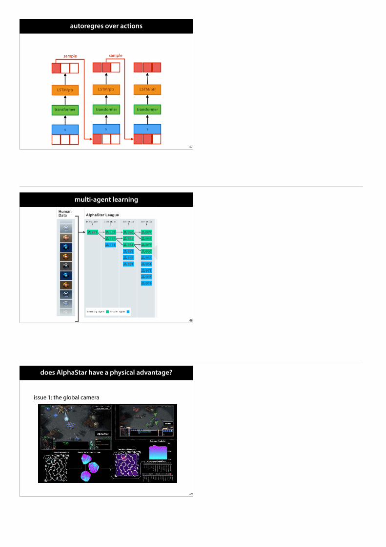
autoregres over actions

67

s

transformer

LSTM/ptr

s

transformer

LSTM/ptr

sample

s

transformer

LSTM/ptr

sample

multi-agent learning

68

does AlphaStar have a physical advantage?

issue 1: the global camera

69

does AlphaStar have a physical advantage?

issue 2: actions-per-minute

70

[email protected] 71

reinforcement learning - mlvu learning.annotated.pdfreinforcement learning problem (although better...

Documents