reinforcement learning or active inference?karl/reinforcement learning or active... ·...
TRANSCRIPT
Reinforcement Learning or Active Inference?Karl J. Friston*, Jean Daunizeau, Stefan J. Kiebel
The Wellcome Trust Centre for Neuroimaging, University College London, London, United Kingdom
Abstract
This paper questions the need for reinforcement learning or control theory when optimising behaviour. We show that it isfairly simple to teach an agent complicated and adaptive behaviours using a free-energy formulation of perception. In thisformulation, agents adjust their internal states and sampling of the environment to minimize their free-energy. Such agentslearn causal structure in the environment and sample it in an adaptive and self-supervised fashion. This results inbehavioural policies that reproduce those optimised by reinforcement learning and dynamic programming. Critically, we donot need to invoke the notion of reward, value or utility. We illustrate these points by solving a benchmark problem indynamic programming; namely the mountain-car problem, using active perception or inference under the free-energyprinciple. The ensuing proof-of-concept may be important because the free-energy formulation furnishes a unified accountof both action and perception and may speak to a reappraisal of the role of dopamine in the brain.
Citation: Friston KJ, Daunizeau J, Kiebel SJ (2009) Reinforcement Learning or Active Inference?. PLoS ONE 4(7): e6421. doi:10.1371/journal.pone.0006421
Editor: Olaf Sporns, Indiana University, United States of America
Received February 12, 2009; Accepted March 19, 2009; Published July 29, 2009
Copyright: � 2009 Friston et al. This is an open-access article distributed under the terms of the Creative Commons Attribution License, which permitsunrestricted use, distribution, and reproduction in any medium, provided the original author and source are credited.
Funding: The Wellcome Trust: Grant#: WT056750; Modelling functional brain architecture. The funders had no role in study design, data collection and analysis,decision to publish, or preparation of the manuscript.
Competing Interests: The authors have declared that no competing interests exist.
* E-mail: [email protected]
Introduction
Traditionally, the optimization of an agent’s behaviour is
formulated as maximizing value or expected reward or utility or
[1–8]. This is seen in cognitive psychology, through the use of
reinforcement learning models like the Rescorla-Wagner model
[1]; in computational neuroscience and machine-learning as
variants of dynamic programming, such as temporal difference
learning [2–7] and in economics, as expected utility theory [8]. In
these treatments, the problem of optimizing behaviour is reduced
to optimizing expected reward or utility (or conversely minimizing
expected loss or cost). Effectively, this prescribes an optimal policy
in terms of the reward that would be expected by pursuing that
policy. Our work suggests that this formulation may represent a
slight misdirection in explaining adaptive behaviour. In this paper,
we specify an optimal policy in terms of the probability distribution
of desired states and ask if this is a simpler and more flexible
approach. Under this specification, optimum behaviour emerges
in agents that conform to a free-energy principle, which provides a
principled basis for understanding both action and perception
[9,10]. In what follows, we review the free-energy principle, show
how it can be used to solve the mountain-car problem [11] and
conclude by considering the implications for the brain and
behaviour.
Methods
The free-energy principleWe start with the premise that adaptive agents or phenotypes
must occupy a limited repertoire of states. See Friston et al [9] for
a detailed discussion: In brief, for a phenotype to exist it must
possess defining characteristics or traits; both in terms of its
morphology and exchange with the environment. These traits
essentially limit the agent to a bounded region in the space of all
states it could be in. Once outside these bounds, it ceases to
possess that trait (cf, a fish out of water). This speaks to self-
organised autopoietic interactions with the world that ensure
phenotypic bounds are never transgressed (cf, [12]). In what
follows, we formalise this notion in terms of the entropy or
average surprise associated with a probability distribution on an
agent’s state-space. The basic idea is that adaptive agents occupy
a compact part of this space and therefore minimise the average
surprise associated with finding itself in unlikely states (cf, a fish
out of water - sic). Starting with this defining attribute of adaptive
agents, we will look at how agents might minimise surprise and
then consider what this entails, in terms of their action and
perception.
The free-energy principle starts with the notion of an ensemble
density p ~xxjt,mð Þ on the generalised states [13], ~xx tð Þ~ x,x’,x’’, . . .f gan agent, m can find itself in. Generalised states cover position,
velocity, acceleration, jerk and so on. We assume these states evolve
according to some complicated equations of motion; _~xx~xx~f ~xx,hð Þz~ww,
where w are random fluctuations, whose amplitude is controlled by
c. Here, h are parameters of a nonlinear function f ~xx,hð Þ, encoding
environmental dynamics. Collectively, causes q6 ~xx,h,cð Þ are all the
environmental quantities that affect the agent, such as forces,
concentrations, rate constants and noise levels. Under these
assumptions, the evolution of the ensemble density is given by the
Fokker-Planck equation
_pp ~xxjt,mð Þ~P h,cð Þp ~xxjt,mð Þ ð1Þ
Where P h,cð Þ~+: V+{f½ � is the Fokker-Planck operator and
V cð Þ is a diffusion tensor corresponding to half the covariance of
~ww. The Fokker-Planck operator plays the role of a probability
transition matrix and determines the ultimate distribution of
states that agents will be found in. The solution to Equation 1, for
PLoS ONE | www.plosone.org 1 July 2009 | Volume 4 | Issue 7 | e6421
which P hð Þp ~xxjmð Þ~0, is the equilibrium density (i.e., when the
density stops changing) and depends only on the parameters
controlling motion and the amplitude of the random fluctuations.
This equilibrium density p ~xxjmð Þ can be regarded as the
probability of finding an agent in a particular state, when
observed on multiple occasions or, equivalently, the density of a
large ensemble of agents at equilibrium with their environment.
Critically, for an agent to exist, the equilibrium density should
have low entropy. As noted above, this ensures that agents
occupy a limited repertoire of states because a low entropy
density has most of its mass in a small part of its support. This
places an important constraint on the states sampled by an agent;
it means agents must somehow minimise their equilibrium
entropy and counter the dispersive effects of random or
deterministic forces. In short, biological agents must resist a
natural tendency to disorder; but how do they do this?
Active agentsAt this point, we introduce the notion of active agents [14] that
sense a subset of states (with sensory organs) and can change others
(with effector organs). We can quantify this exchange with the
environment with sensory, ~ss tð Þ~ s,s’,s’’, . . .f g and action or
control signals, a(t). We will describe sensory sampling (e.g.,
retinotopic encoding) as a probabilistic mapping, ~ss~g ~xx,hð Þz~zz,
where z is sensory noise. Control (e.g., saccadic eye-movements)
can be represented by treating action as a state; a5~xx; which we
will call hidden states from now on because they are not sensed
directly. From the point of view of reinforcement learning and
optimum control theory, action depends on sensory signals, where
this dependency constitutes a policy, a~p ~ssð Þ.Under a sensory mapping, the equilibrium entropy is bounded
by the entropy of sensory signals minus a sensory transfer term
H ~xxð ÞƒH ~ssð Þ{ð
p ~xxð ÞlnjLg=L~xxjd~xx
H ~ssð Þ~{
ðp ~ssjmð Þln ~ssjmð Þd~ss
H ~xxð Þ~{
ðp ~xxjmð Þln p ~xxjmð Þd~xx
ð2Þ
with equality in the absence of sensory noise. This means it is
sufficient to minimise the terms on the right to minimise the
equilibrium entropy of hidden states. The second term depends on
the sensitivity of sensory inputs to changes in the agent’s states,
where Lg=L~xx is the derivative of the sensory mapping with respect
to generalised hidden states. Minimising this term maximises the
mutual information between hidden states and sensory signals.
This recapitulates the principle of maximum information transfer
[15], which has been very useful in understanding things like
receptive fields [16]. Put simply, sensory channels should match
the dynamic range of states they sample (e.g., the spectral
sensitivity profile of photoreceptors and the spectrum of ambient
light).
In the present context, the interesting term is the sensory
entropy; H ~ssð Þ, which can be minimised through action because
sensory signals depend upon hidden states, which include action.
The argument here is that it is necessary but not sufficient to
minimise the entropy of the sensory signals. To ensure the
entropy of the hidden states per se is minimised one has to assume
the agent is equipped with (and uses) its sensory apparatus to
maximise information transfer. We will assume this is assured
through natural selection and focus on the minimisation of
sensory entropy:
Crucially, because the density on sensory signals is at
equilibrium, it can be interpreted as the proportion of time each
agent entertains these signals (this is called the sojourn time). This
ergodic argument [17] means that the ensemble entropy is the
long-term average or path integral of {ln p ~ssjmð Þ experienced by
any particular agent:
H ~ssð Þ~ limT??
{1
T
ðT0
ln p ~ss tð Þjmð Þdt ð3Þ
In other words, active agents minimise {ln p ~ss,mð Þ over time
(by the fundamental lemma of the calculus of variations). This
quantity is known as self-information or surprise in information
theory (and as the negative log-evidence in statistics). When
friends and colleagues first come across this conclusion, they
invariably respond with; ‘‘but that means I should just close my
eyes or head for a dark room and stay there’’. In one sense this is
absolutely right; and is a nice description of going to bed.
However, this can only be sustained for a limited amount of time,
because the world does not support, in the language of dynamical
systems, stable fixed-point attractors. At some point you will
experience surprising states (e.g., dehydration or hypoglycaemia).
More formally, itinerant dynamics in the environment preclude
simple solutions to avoiding surprise; the best one can do is to
minimise surprise in the face of stochastic and chaotic sensory
perturbations. In short, a necessary condition for an agent to exist
is that it adopts a policy that minimizes surprise. However, there
is a problem:
The need for perceptionThe problem faced by real agents is that they cannot quantify
surprise, which entails marginalizing over the unknown causes,
q6 ~xx,h,cf g of sensory input
{ln p ~ssjmð Þ~{ln
ðp ~ss,qjmð Þdq ð4Þ
However, there is an alternative and elegant solution to
minimizing surprise, which comes from theoretical physics [18]
and machine learning [19,20]. This involves minimizing a free-
energy bound on surprise that can be evaluated (minimising the
bound implicitly minimises surprise because the bound is always
greater than surprise). This bound is induced by a recognition
density; q q : mð Þ, whose sufficient statistics m are, we assume,
encoded by the internal states of the agent (e.g., neuronal activity
or metabolite concentrations and connection strengths or rate-
constants). The recognition density is a slightly mysterious
construct because it is an arbitrary probability density specified by
the internal states of the agent. Its role is to induce free-energy,
which is a function of the internal states and sensory inputs. We
will see below that when this density is optimised to minimise free-
energy it becomes the conditional density on the causes of sensory
data; in Bayesian inference this is known as the recognition
density. In what follows, we try to summarise the key ideas behind
a large body of work in statistics and machine learning referred to
as ensemble learning or variational Bayes.
Active Inference
PLoS ONE | www.plosone.org 2 July 2009 | Volume 4 | Issue 7 | e6421
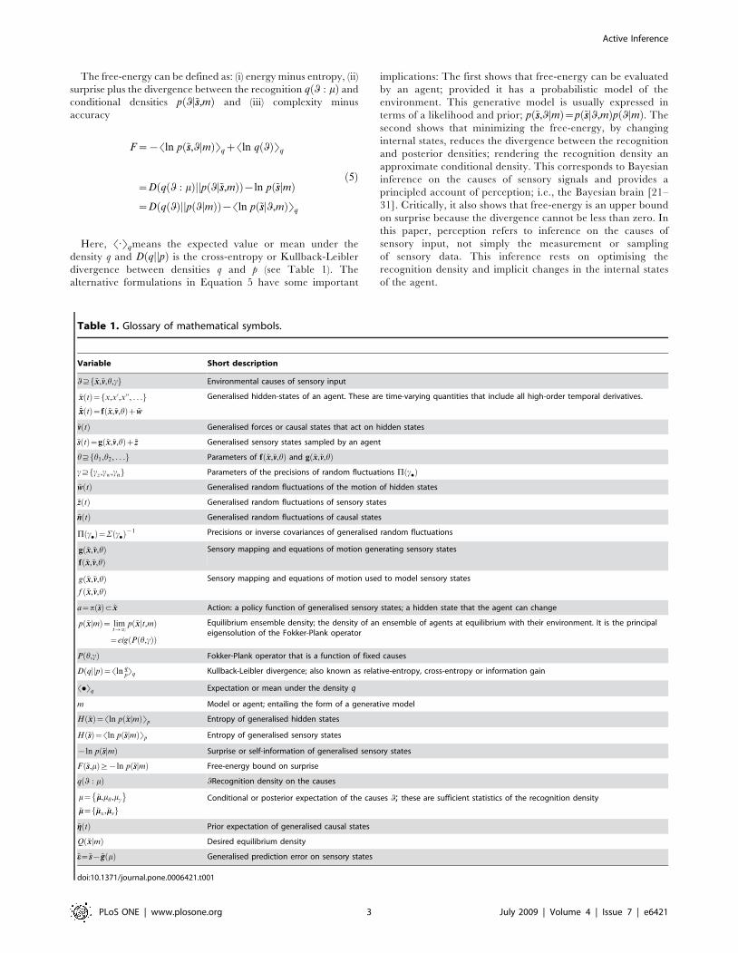
The free-energy can be defined as: (i) energy minus entropy, (ii)
surprise plus the divergence between the recognition q q : mð Þ and
conditional densities p qj~ss,mð Þ and (iii) complexity minus
accuracy
F~{Sln p ~ss,qjmð ÞTqzSln q qð ÞTq
~D q q : mð Þjjp qj~ss,mð Þð Þ{ln p ~ssjmð Þ
~D q qð Þjjp qjmð Þð Þ{Sln p ~ssjq,mð ÞTq
ð5Þ
Here, S:Tqmeans the expected value or mean under the
density q and D qjjpð Þ is the cross-entropy or Kullback-Leibler
divergence between densities q and p (see Table 1). The
alternative formulations in Equation 5 have some important
implications: The first shows that free-energy can be evaluated
by an agent; provided it has a probabilistic model of the
environment. This generative model is usually expressed in
terms of a likelihood and prior; p ~ss,qjmð Þ~p ~ssjq,mð Þp qjmð Þ. The
second shows that minimizing the free-energy, by changing
internal states, reduces the divergence between the recognition
and posterior densities; rendering the recognition density an
approximate conditional density. This corresponds to Bayesian
inference on the causes of sensory signals and provides a
principled account of perception; i.e., the Bayesian brain [21–
31]. Critically, it also shows that free-energy is an upper bound
on surprise because the divergence cannot be less than zero. In
this paper, perception refers to inference on the causes of
sensory input, not simply the measurement or sampling
of sensory data. This inference rests on optimising the
recognition density and implicit changes in the internal states
of the agent.
Table 1. Glossary of mathematical symbols.
Variable Short description
q) ~xx,~vv,h,cf g Environmental causes of sensory input
~xx tð Þ~ x,x’,x’’, . . .f g_~xx~xx tð Þ~f ~xx,~vv,hð Þz~ww
Generalised hidden-states of an agent. These are time-varying quantities that include all high-order temporal derivatives.
~vv tð Þ Generalised forces or causal states that act on hidden states
~ss tð Þ~g ~xx,~vv,hð Þz~zz Generalised sensory states sampled by an agent
h) h1,h2, . . .f g Parameters of f ~xx,~vv,hð Þ and g ~xx,~vv,hð Þc) cz,cw,cnf g Parameters of the precisions of random fluctuations P c.ð Þ~ww tð Þ Generalised random fluctuations of the motion of hidden states
~zz tð Þ Generalised random fluctuations of sensory states
~nn tð Þ Generalised random fluctuations of causal states
P c.ð Þ~S c.ð Þ{1 Precisions or inverse covariances of generalised random fluctuations
g ~xx,~vv,hð Þf ~xx,~vv,hð Þ
Sensory mapping and equations of motion generating sensory states
g ~xx,~vv,hð Þf ~xx,~vv,hð Þ
Sensory mapping and equations of motion used to model sensory states
a~p ~ssð Þ5~xx Action: a policy function of generalised sensory states; a hidden state that the agent can change
p ~xx mjð Þ~ limt??
p ~xxjt,mð Þ
~eig P h,cð Þð Þ
Equilibrium ensemble density; the density of an ensemble of agents at equilibrium with their environment. It is the principaleigensolution of the Fokker-Plank operator
P h,cð Þ Fokker-Plank operator that is a function of fixed causes
D qjjpð Þ~Sln qpTq Kullback-Leibler divergence; also known as relative-entropy, cross-entropy or information gain
S.Tq Expectation or mean under the density q
m Model or agent; entailing the form of a generative model
H ~xxð Þ~Sln p ~xxjmð ÞTp Entropy of generalised hidden states
H ~ssð Þ~Sln p ~ssjmð ÞTp Entropy of generalised sensory states
{ln p ~ssjmð Þ Surprise or self-information of generalised sensory states
F ~ss,mð Þ§{ln p ~ssjmð Þ Free-energy bound on surprise
q q : mð Þ qRecognition density on the causes
m~ ~mm,mh,mc
� �~mm~ ~mmx,~mmvf g
Conditional or posterior expectation of the causes q; these are sufficient statistics of the recognition density
~gg tð Þ Prior expectation of generalised causal states
Q ~xxjmð Þ Desired equilibrium density
~ee~~ss{~gg mð Þ Generalised prediction error on sensory states
doi:10.1371/journal.pone.0006421.t001
Active Inference
PLoS ONE | www.plosone.org 3 July 2009 | Volume 4 | Issue 7 | e6421
The third equality shows that free-energy can also be suppressed
by action, through its vicarious effects on sensory signals. In short, the
free-energy principle prescribes perception and an optimum policy
m~ arg minm
F ~ss,mð Þ
a~p ~ss,mð Þ~ arg mina
F ~ss,mð Þð6Þ
This policy reduces to sampling input that is expected under the
recognition density (i.e., sampling selectively what one expects to
see, so that accuracy is maximised; Equation 5). In other words,
agents must necessarily (if implicitly) make inferences about the
causes of their sensory signals and sample those that are consistent
with those inferences. This is similar to the notion that ‘‘perception
and behaviour can interact synergistically, via the environment’’ to
optimise behaviour [32]. Furthermore, it echoes recent perspec-
tives on sequence learning that ‘‘minimize deviations from the
desired state, that is, to minimize disturbances of the homeostasis
of the feedback loop’’. See Worgotter & Porr [33] for a fuller
discussion.
At first glance, sampling the world to ensure it conforms
to our expectations may seem to preclude exploration or
sampling salient information. However, the minimisation in
Equation 6 could use a stochastic search; sampling the
sensorium randomly for a percept with low free-energy. Indeed,
there is compelling evidence that our eye movements implement
an optimal stochastic strategy [34]. This raises interesting
questions about the role of stochastic schemes; from visual
search to foraging. However, in this treatment, we will focus on
gradient descent.
SummaryIn summary, the free-energy principle requires the internal
states of an agent and its action to suppress free-energy. This
corresponds to optimizing a probabilistic model of how
sensations are caused, so that the ensuing predictions can guide
active sampling of sensory data. The resulting interplay between
action and perception (i.e., active inference) engenders a policy
that ensures the agent’s equilibrium density has low entropy. Put
simply, if you search out things you expect, you will avoid
surprises. It is interesting that the second law of thermodynamics
(which applies only to closed systems) can be resisted by
appealing to the more general tendency of (open) systems to
reduce their free-energy [35,36]. However, it is important not to
confuse the free-energy here with thermodynamic free-energy in
physics. Variational free-energy is an information theory
measure that is a scalar function of sensory states or data and a
probability density (the recognition density). This means
thermodynamic arguments are replaced by arguments based on
population dynamics (see above), when trying to understand why
agents minimise their free-energy. A related, if abstract,
treatment of self-organisation in non-equilibrium systems can
be found in synergetics; where ‘‘patterns become functional
because they consume in a most efficient manner the gradients
which cause their evolution’’ [37]. Here, these gradients can be
regarded as surprise. Finally, Distributed Adaptive Control [38]
also relates closely to the free-energy formulation, because it
addresses the optimisation of priors and provides an integrated
solution to both the acquisition of state-space models and
policies, without relying on reward or value signals: see [32]
and [38].
Active inferenceTo see how active inference works in practice, one must first
define an environment and the agent’s model of that environment.
We will assume that both can be cast as dynamical systems with
additive random effects. For the environment we have
~ss~g ~xx,~vv,a,hð Þz~zz
_~xx~xx~f ~xx,~vv,a,hð Þz~wwð7Þ
which is modelled as
~ss~g ~xx,~vv,hð Þz~zz
_~xx~xx~f ~xx,~vv,hð Þz~ww
~vv~~ggz~nn
ð8Þ
These stochastic differential equations describe how sensory
inputs are generated as a function of hidden generalized states, ~xxand exogenous forces, ~vv plus sensory noise, ~zz. Note that we
partitioned hidden states into hidden states and forces so that
q6 ~xx,~vv,a,hf g. The hidden states evolve according to some
equations of motion plus state noise, ~ww. The use of generalised
coordinates may seem a little redundant, in the sense that one
might use a standard Langevin form for the stochastic differential
equations above. However, we do not assume the random
fluctuations are Weiner processes and allow for temporally
correlated noise. This induces a finite variance on all higher
derivatives of the fluctuations and necessitates the use of
generalised coordinates. Although generalised coordinates may
appear to complicate matters, they actually simplify inference
greatly; see [13] and [39] for details.
Gaussian assumptions about the random fluctuations furnish a
likelihood model; p ~ssjqð Þ~N g,S czð Þð Þ and, critically, priors on the
dynamics, p _~xx~xxj~vv,h� �
~N f ,S cwð Þð Þ. Here the inverse covariances or
precisions c6 cz,cwf g determine the amplitude and smoothness of
the generalised fluctuations. Note that the true states depend on
action, whereas the generative model has no notion of action; it
just produces predictions that action tries to fulfil. Furthermore,
the generative model contains a prior on the exogenous forces;
p ~vvð Þ~N ~gg,S cnð Þð Þ. Here, c6cn is the precision of the noise on the
forces, ~nn and is effectively a prior precision. It is important to
appreciate that the equations actually generating data (Equation 7)
and those employed by the generative model (Equation 8) do not
have to be the same; indeed, it is this discrepancy that action tries
to conceal. Given a specific form for the generative model the free-
energy can now be optimised:
This optimisation obliges the agent to infer the states of the
world and learn the unknown parameters responsible for its
motion by optimising the sufficient statistics of its recognition
density; i.e., perceptual inference and learning. This can be
implemented in a biologically plausible fashion using a principle of
stationary action as described in [39]. In brief, this scheme
assumes a mean-field approximation; q qð Þ~q ~xx,~vvð Þq hð Þq cð Þ with
Gaussian marginals, whose sufficient statistics are expectations and
covariances. Under this Gaussian or Laplace assumption, it is
sufficient to optimise the expectations, m~ ~mmx,~mmv,mh,mc
� �because
they specify the covariances in closed form. Using these
assumptions, we can formulate Equation 6 as a gradient descent
that describes the dynamics of perceptual inference, learning and
action:
Active Inference
PLoS ONE | www.plosone.org 4 July 2009 | Volume 4 | Issue 7 | e6421
_~mm~mmx~D~mmx{+~xxF
_~mm~mmv~D~mmv{+~vvF
€mmh~{+hF
€mmc~{+cF
_aa~{+aF~{+a~eeTP~ee
ð9Þ
We now unpack these equations and what they mean. The top-
two equations prescribe recognition dynamics on expected states
of the world. The second terms of these equations are simply free-
energy gradients. The first terms reflect the fact that we are
working in generalised coordinates and ensure _~mm~mm~D~mm when free-
energy is minimised and its gradient is zero (i.e., the motion of the
expectations is the expected motion). Here, D is a derivative
operator with identity matrices in the first leading diagonal. The
solutions to the next pair of equations are the optimum parameters
and precisions. Note that these are second-order differential
equations because these expectations optimise a path-integral of
free-energy; see [13] for details. The final equation describes
action as a gradient descent on free-energy. Recall that the only
way action can affect free-energy is through sensory signals. This
means, under the Laplace assumption, action must suppress
prediction error; ~ee~~ss að Þ{g ~mmð Þ at the sensory level; where P mzc
� �is the expected precision of sensory noise.
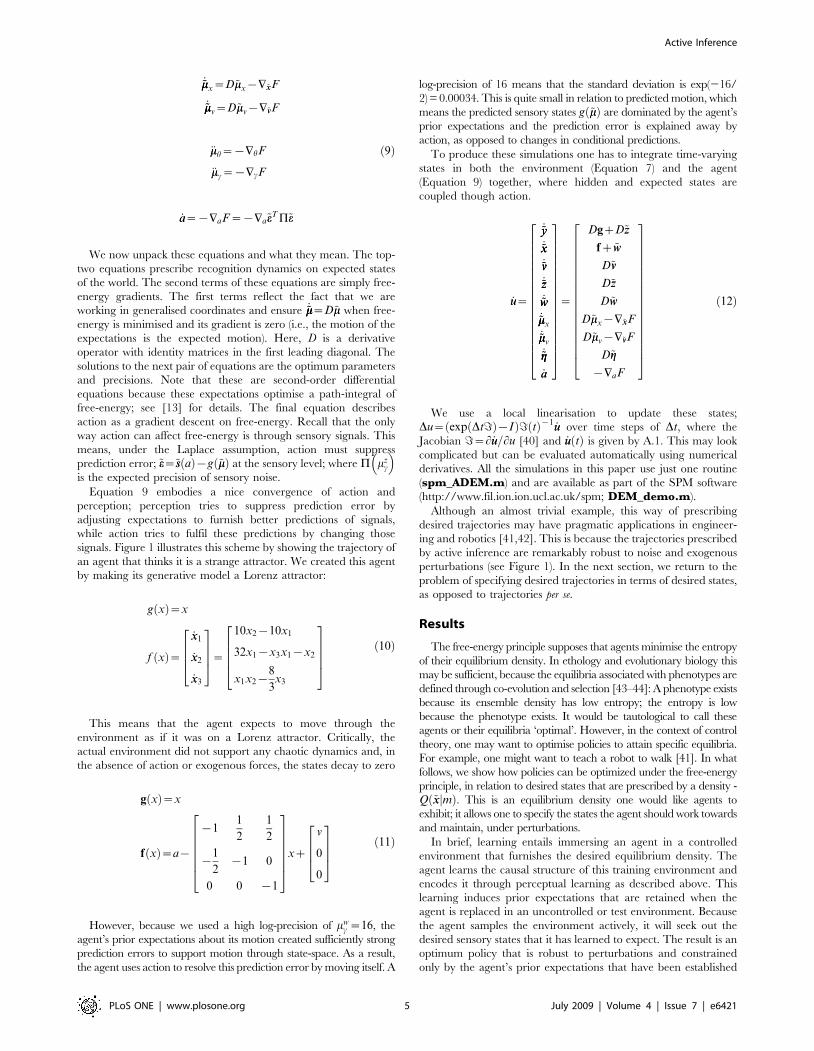
Equation 9 embodies a nice convergence of action and
perception; perception tries to suppress prediction error by
adjusting expectations to furnish better predictions of signals,
while action tries to fulfil these predictions by changing those
signals. Figure 1 illustrates this scheme by showing the trajectory of
an agent that thinks it is a strange attractor. We created this agent
by making its generative model a Lorenz attractor:
g xð Þ~x
f xð Þ~
_xx1
_xx2
_xx3
2664
3775~
10x2{10x1
32x1{x3x1{x2
x1x2{8
3x3
26664
37775
ð10Þ
This means that the agent expects to move through the
environment as if it was on a Lorenz attractor. Critically, the
actual environment did not support any chaotic dynamics and, in
the absence of action or exogenous forces, the states decay to zero
g xð Þ~x
f xð Þ~a{
{11
2
1
2
{1
2{1 0
0 0 {1
2666664
3777775xz
v
0
0
26643775 ð11Þ
However, because we used a high log-precision of mwc ~16, the
agent’s prior expectations about its motion created sufficiently strong
prediction errors to support motion through state-space. As a result,
the agent uses action to resolve this prediction error by moving itself. A
log-precision of 16 means that the standard deviation is exp(216/
2) = 0.00034. This is quite small in relation to predicted motion, which
means the predicted sensory states g ~mmð Þ are dominated by the agent’s
prior expectations and the prediction error is explained away by
action, as opposed to changes in conditional predictions.
To produce these simulations one has to integrate time-varying
states in both the environment (Equation 7) and the agent
(Equation 9) together, where hidden and expected states are
coupled though action.
_uu~
_~yy~yy_~xx~xx_~vv~vv
_~zz~zz
_~ww~ww
_~mm~mmx
_~mm~mmv
_~gg~gg
_aa
266666666666666664
377777777777777775
~
DgzD~zz
fz~ww
D~vv
D~zz
D~ww
D~mmx{+~xxF
D~mmv{+~vvF
D~gg
{+aF
266666666666666664
377777777777777775
ð12Þ
We use a local linearisation to update these states;
Du~ exp Dt=ð Þ{Ið Þ= tð Þ{1 _uu over time steps of Dt, where the
Jacobian =~L _uu=Lu [40] and _uu tð Þ is given by A.1. This may look
complicated but can be evaluated automatically using numerical
derivatives. All the simulations in this paper use just one routine
(spm_ADEM.m) and are available as part of the SPM software
(http://www.fil.ion.ion.ucl.ac.uk/spm; DEM_demo.m).
Although an almost trivial example, this way of prescribing
desired trajectories may have pragmatic applications in engineer-
ing and robotics [41,42]. This is because the trajectories prescribed
by active inference are remarkably robust to noise and exogenous
perturbations (see Figure 1). In the next section, we return to the
problem of specifying desired trajectories in terms of desired states,
as opposed to trajectories per se.
Results
The free-energy principle supposes that agents minimise the entropy
of their equilibrium density. In ethology and evolutionary biology this
may be sufficient, because the equilibria associated with phenotypes are
defined through co-evolution and selection [43–44]: A phenotype exists
because its ensemble density has low entropy; the entropy is low
because the phenotype exists. It would be tautological to call these
agents or their equilibria ‘optimal’. However, in the context of control
theory, one may want to optimise policies to attain specific equilibria.
For example, one might want to teach a robot to walk [41]. In what
follows, we show how policies can be optimized under the free-energy
principle, in relation to desired states that are prescribed by a density -
Q ~xxjmð Þ. This is an equilibrium density one would like agents to
exhibit; it allows one to specify the states the agent should work towards
and maintain, under perturbations.
In brief, learning entails immersing an agent in a controlled
environment that furnishes the desired equilibrium density. The
agent learns the causal structure of this training environment and
encodes it through perceptual learning as described above. This
learning induces prior expectations that are retained when the
agent is replaced in an uncontrolled or test environment. Because
the agent samples the environment actively, it will seek out the
desired sensory states that it has learned to expect. The result is an
optimum policy that is robust to perturbations and constrained
only by the agent’s prior expectations that have been established
Active Inference
PLoS ONE | www.plosone.org 5 July 2009 | Volume 4 | Issue 7 | e6421
during training. To create a controlled environment one can
simply minimise the divergence between the uncontrolled
equilibrium density and the desired density. We now illustrate
this form of learning using a ubiquitous example from dynamic
programming - the mountain-car problem.
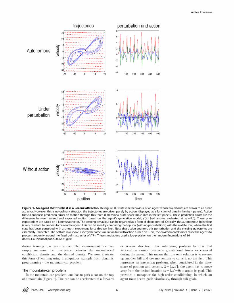
The mountain-car problemIn the mountain-car problem, one has to park a car on the top
of a mountain (Figure 2). The car can be accelerated in a forward
or reverse direction. The interesting problem here is that
acceleration cannot overcome gravitational forces experienced
during the ascent. This means that the only solution is to reverse
up another hill and use momentum to carry it up the first. This
represents an interesting problem, when considered in the state-
space of position and velocity, ~xx~ x,x’f g; the agent has to move
away from the desired location (x~1,x’~0) to attain its goal. This
provides a metaphor for high-order conditioning, in which an
agent must access goals vicariously, through sub-goals.
Figure 1. An agent that thinks it is a Lorenz attractor. This figure illustrates the behaviour of an agent whose trajectories are drawn to a Lorenzattractor. However, this is no ordinary attractor; the trajectories are driven purely by action (displayed as a function of time in the right panels). Actiontries to suppress prediction errors on motion through this three dimensional state-space (blue lines in the left panels). These prediction errors are thedifference between sensed and expected motion based on the agent’s generative model; f ~xxð Þ (red arrows: evaluated at x3~0:5). These priorexpectations are based on a Lorentz attractor. The ensuing behaviour can be regarded as a form of chaos control. Critically, this autonomous behaviouris very resistant to random forces on the agent. This can be seen by comparing the top row (with no perturbations) with the middle row, where the firststate has been perturbed with a smooth exogenous force (broken line). Note that action counters this perturbation and the ensuing trajectories areessentially unaffected. The bottom row shows exactly the same simulation but with action turned off. Here, the environmental forces cause the agents toprecess randomly around the fixed point attractor of f ~xxð Þ. These simulations used a log-precision on the random fluctuations of 16.doi:10.1371/journal.pone.0006421.g001
Active Inference
PLoS ONE | www.plosone.org 6 July 2009 | Volume 4 | Issue 7 | e6421
The mountain-car environment can be specified with the
sensory mapping and equations of motions (where 6 denotes the
Kronecker tensor product)
g~~xx
f~_xx
_xx’
" #~
x’
{b{1
4x’zvzs azcð Þ
24
35
b~2xz1 : xƒ0
1z5x2� �{1=2
{5x2 1z5x2� �{3=2
{ x=2ð Þ4 : xw0
(
c~h1zh2~xxzh3 ~xx6~xxð Þ
ð13Þ
The first equality means the car has a (noisy) sense of its position
and velocity. The second means that the forces on the car, _xx’ have
four components: a gravitational force b, friction {x’=4, an
exogenous force v and a force that is bounded by a squashing
(logistic) function; {1ƒsƒ1. The latter force comprises action
and a state-dependent control, c. Control is approximated here
with a second-order polynomial expansion of any nonlinear
function of the states, whose parameters are h~ h1,h2,h3f g. When
h~0 the environment is uncontrolled; otherwise the car
experiences state-dependent forces that enable control.
To create a controlled environment that leads to an optimum
equilibrium, we simply optimise the parameters to minimise the
divergence between the equilibrium and desired densities; i.e.
hQ~ arg minh
D Q ~xxjmð Þjjp ~xxjmð Þð Þ
D Q ~xxjmð Þjjp ~xxjmð Þð Þ~ð
Q ~xxjmð Þln Q ~xxjmð Þeig P h,cð Þð Þd~xx
ð14Þ
The equilibrium density is the eigensolution p ~xxjmð Þ~eig P h,cð Þð Þof the Fokker-Planck operator in Equation 1, which depends on the
parameters and the precision of random fluctuations (we assumed
these had a log-precision of 16). We find these eigensolutions by
iterating Equation 1 until convergence to avoid inverting large
matrices. The minimization above can use any nonlinear function
minimization or optimization scheme; such as Nelder-Mead.
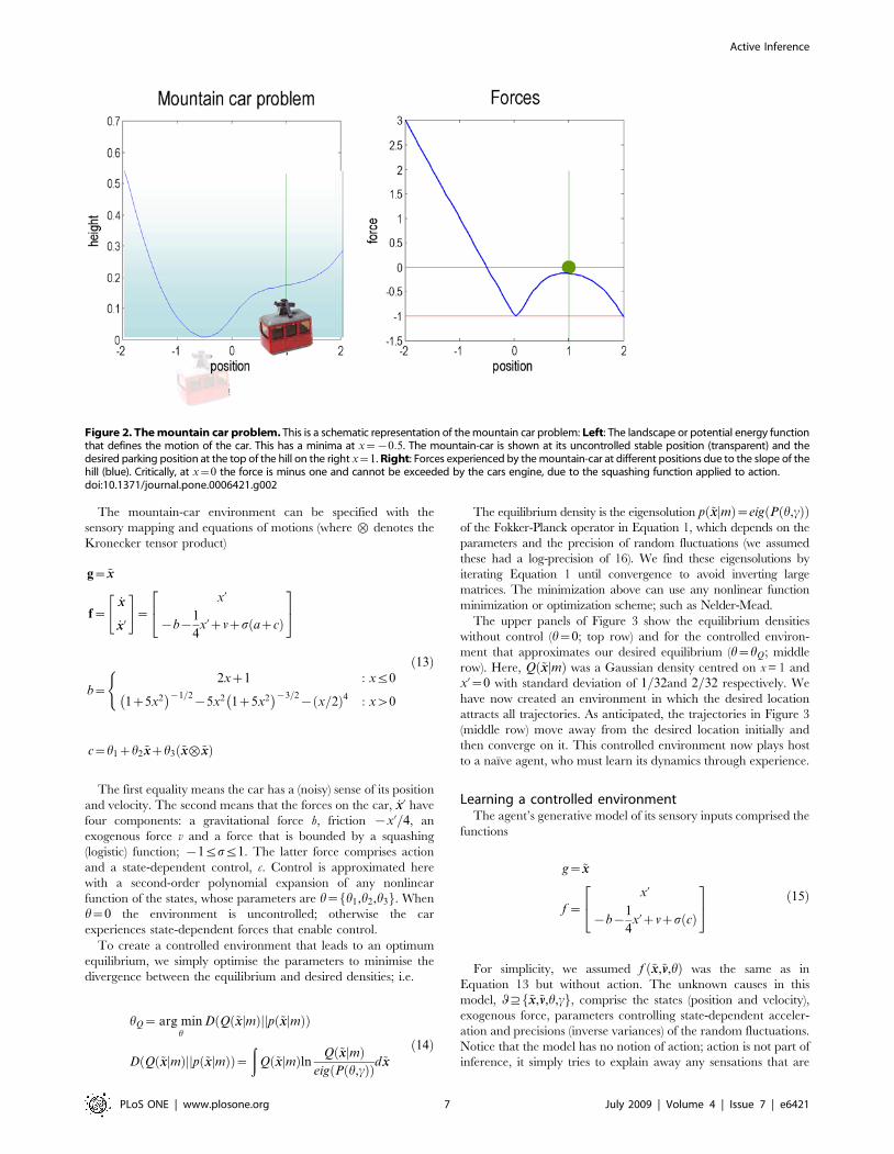
The upper panels of Figure 3 show the equilibrium densities
without control (h~0; top row) and for the controlled environ-
ment that approximates our desired equilibrium (h~hQ; middle
row). Here, Q ~xxjmð Þ was a Gaussian density centred on x = 1 and
x’~0 with standard deviation of 1=32and 2=32 respectively. We
have now created an environment in which the desired location
attracts all trajectories. As anticipated, the trajectories in Figure 3
(middle row) move away from the desired location initially and
then converge on it. This controlled environment now plays host
to a naıve agent, who must learn its dynamics through experience.
Learning a controlled environmentThe agent’s generative model of its sensory inputs comprised the
functions
g~~xx
f ~
x’
{b{1
4x’zvzs cð Þ
24
35 ð15Þ
For simplicity, we assumed f ~xx,~vv,hð Þ was the same as in
Equation 13 but without action. The unknown causes in this
model, q) ~xx,~vv,h,cf g, comprise the states (position and velocity),
exogenous force, parameters controlling state-dependent acceler-
ation and precisions (inverse variances) of the random fluctuations.
Notice that the model has no notion of action; action is not part of
inference, it simply tries to explain away any sensations that are
Figure 2. The mountain car problem. This is a schematic representation of the mountain car problem: Left: The landscape or potential energy functionthat defines the motion of the car. This has a minima at x~{0:5. The mountain-car is shown at its uncontrolled stable position (transparent) and thedesired parking position at the top of the hill on the right x~1. Right: Forces experienced by the mountain-car at different positions due to the slope of thehill (blue). Critically, at x~0 the force is minus one and cannot be exceeded by the cars engine, due to the squashing function applied to action.doi:10.1371/journal.pone.0006421.g002
Active Inference
PLoS ONE | www.plosone.org 7 July 2009 | Volume 4 | Issue 7 | e6421
Figure 3. Equilibria in the state-space of the mountain car problem. Left panels: Flow-fields and associated equilibria for an uncontrolledenvironment (top), a controlled or optimised environment (middle) and under prior expectations after learning (bottom). Notice how the flow ofstates in the controlled environment enforces trajectories that start by moving away from the desired location (green dot at x~1). The arrows denotethe flow of states (position and velocity) prescribed by the parameters. The equilibrium density in each row is the principal eigenfunction of theFokker-Plank operator associated with the parameters. For the controlled and expected environments, these are low entropy equilibria, centred onthe desired location. Right panels: These panels show the flow fields in terms of their nullclines. Nullclines correspond to lines in state-space wherethe rate of change or one variable is zero. Here the nullcline for position is along the x-axis, where velocity is zero. The nullcline for velocity is whenthe change in velocity goes from positive (grey) to negative (white). Fixed points correspond to the intersection of these nullclines. It can be seen thatunder an uncontrolled environment (top) there a stable fixed point, where the velocity nullcline intersects the position nullcline with negative slope.Under controlled (middle) and expected (bottom) dynamics there are three fixed points. The rightmost fixed-point is under the desired equilibriumdensity and is stable. The middle fixed-point is halfway up the hill and the final fixed-point is at the bottom. Both of these are unstable and repeltrajectories so that they are ultimately attracted to the desired location. The red lines depict exemplar trajectories, under deterministic flow, fromx~x’~0. In a controlled environment, this shows the optimum behaviour of moving up the opposite hill to gain momentum so that the desiredlocation can be reached.doi:10.1371/journal.pone.0006421.g003
Active Inference
PLoS ONE | www.plosone.org 8 July 2009 | Volume 4 | Issue 7 | e6421
not predicted. The agent was exposed to 16 trials of 32 second
time-bins. Simulated training involved integrating Equation 12
with h~hQ. On each trial, the car was ‘pushed’ with an exogenous
force, sampled from a Gaussian density with a standard deviation
of eight. This enforced a limited exploration of state-space. The
agent was aware of these perturbations, which entered as priors on
the forcing term; i.e. ~gg~~vv (see Equation 8). During learning, we
precluded active inference, a = 0; such that the agent sensed its
trajectory passively, as it was expelled from the desired state and
returned to it.
Note that the agent does know the true states because we added
a small amount of observation error (with a log-precision of eight)
to form sensory inputs. Furthermore, the agent’s model allows for
random fluctuations on both position and velocity. When
generating sensory data we used a small amount of noise on the
motion of the velocity (log-precision of eight). After 16 trials the
parameters converged roughly to the values used to construct the
control environment. This means, in effect, the agent expects to be
delivered, under state-dependent forces, to the desired state. These
optimum dynamics have been learned in terms of (empirical)
priors on the generalised motion of states encoded by mh, the
expected parameters of the equations of motion. These expecta-
tions are shown in the lower row of Figure 3 in term of trajectories
encoded by f ~xx,~vv,mhð Þ. It can be seen that the nullclines (lower
right) based on the parameters after training have a similar
topology to the controlled environment (middle right), ensuring
the fixed-points that have been learnt are the same as those
desired. So what would happen if the agent was placed in an
uncontrolled environment that did not conform to its expecta-
tions?
Active inferenceTo demonstrate the agent has learnt the optimum policy, we
placed it in an uncontrolled environment; i.e., h~0 and allowed
action to minimize free-energy. Although it would be interesting to
see the agent adapt to the uncontrolled environment, we
precluded any further perceptual learning. An example of active
inference after learning is presented in Figure 4. Again this
involved integrating environmental and recognition dynamics
(Equations 7 and 9); where these stochastic differential equations
are now coupled through action (Equation 12). The coloured lines
show the conditional expectations of the states, while the grey
areas represent 90% confidence intervals. These are very tight
because we used low levels of noise. The dotted red line on the
upper left corresponds to the prediction error; namely the
discrepancy between the observed and predicted states. The
ensuing trajectory is superimposed on the nullclines and shows the
agent moving away from its goal initially; to build up the
momentum required to ascend the hill. Once the goal has been
attained action is still required because, in the test environment, it
is not a fixed-point attractor.
To illustrate the robustness of this behaviour, we repeated the
simulation using a smooth exogenous perturbation (e.g., a strong
wind, modelled with a random normal variate, smoothed with a
Gaussian kernel of eight seconds). Because the agent did not
expect this, it was explained away by action and not perceived.
The ensuing goal-directed behaviour was preserved under this
perturbation (lower panels of Figure 4). Note the mirror
symmetry between action and the displacing force it counters
(action is greater because it exerts its effects through a squashing
function).
In this example, we made things easy for the agent by giving it
the true form of the process generating its sensory data. This
meant the agent only had to learn the parameters. In a more
general setting, agents have to learn both the form and parameters
of their generative models. However, there is no fundamental
distinction between learning the form and parameters of a model,
because the form can be cast in terms of priors that switch
parameters on or off (c.f., automatic relevance determination and
model optimisation; [45]). In brief, this means that optimising the
parameters (and hyperparameters) of a model can be used to
optimise its form. Indeed, in statistics, Bayesian model selection is
based upon a free-energy bound on the log-evidence for
competing models [46]. They key thing here is that the free-
energy principle reduces the problem of learning an optimum
policy to the much simpler and well-studied problem of perceptual
learning, without reference to action. Optimum control emerges
when active inference is engaged.
Optimal behaviour and conditional confidenceOptimal behaviour depends on the precision of expected
motion of the hidden states encoded by mwc . In this example, the
agent was fairly confident about its prior expectations but did not
discount sensory evidence completely (with log-precisions of
mwc ~mz
c~8). These conditional precisions are important quanti-
ties and control the relative influence of bottom-up sensory
information relative to top-down predictions. In a perceptual
setting they mediate attentional gain; c.f., [9,47,48]. In active
inference, they also control whether an action is emitted or not
(i.e., motor intention): Increasing the relative precision of
empirical priors on motion causes more confident behaviour,
whereas reducing it subverts action, because prior expectations
are overwhelmed by sensory input and are therefore not
expressed at the level of sensory predictions. In biological
formulations of the free-energy principle, current thinking is that
dopamine might encode the precision of prior expectations
[39,48]. A deficit in dopaminergic neurotransmission would
reduce the operational potency of priors to elicit action and lead
to motor poverty; as seen in Parkinson’s disease, schizophrenia
and neuroleptic bradykinesia.
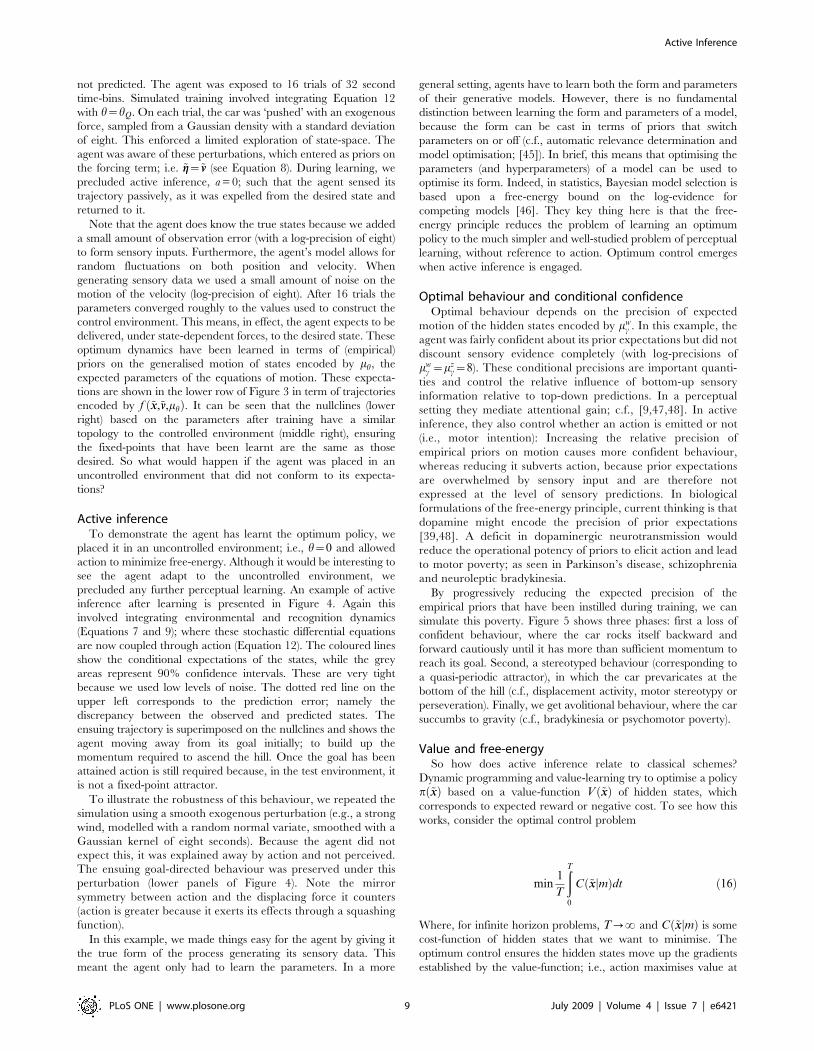
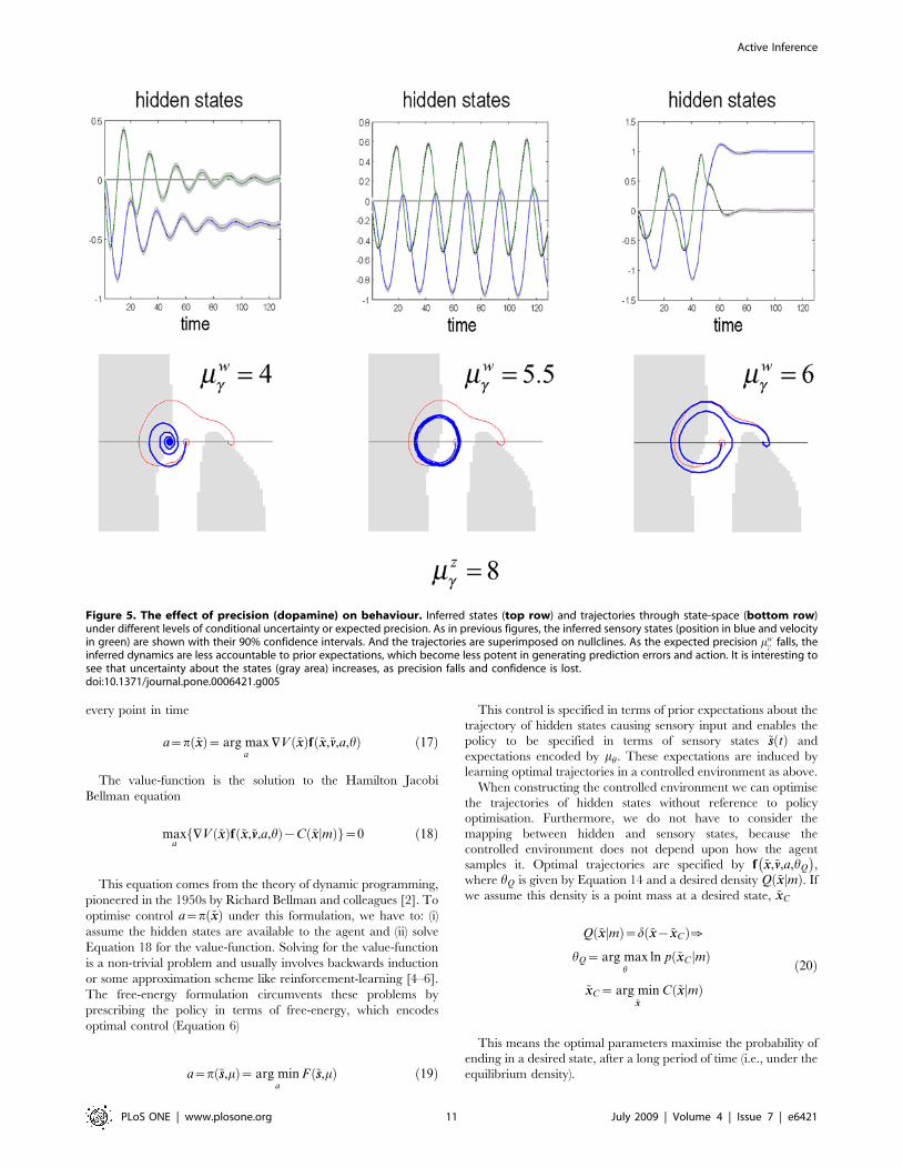
By progressively reducing the expected precision of the
empirical priors that have been instilled during training, we can
simulate this poverty. Figure 5 shows three phases: first a loss of
confident behaviour, where the car rocks itself backward and
forward cautiously until it has more than sufficient momentum to
reach its goal. Second, a stereotyped behaviour (corresponding to
a quasi-periodic attractor), in which the car prevaricates at the
bottom of the hill (c.f., displacement activity, motor stereotypy or
perseveration). Finally, we get avolitional behaviour, where the car
succumbs to gravity (c.f., bradykinesia or psychomotor poverty).
Value and free-energySo how does active inference relate to classical schemes?
Dynamic programming and value-learning try to optimise a policy
p ~xxð Þ based on a value-function V ~xxð Þ of hidden states, which
corresponds to expected reward or negative cost. To see how this
works, consider the optimal control problem
min1
T
ðT0
C ~xxjmð Þdt ð16Þ
Where, for infinite horizon problems, T?? and C ~xxjmð Þ is some
cost-function of hidden states that we want to minimise. The
optimum control ensures the hidden states move up the gradients
established by the value-function; i.e., action maximises value at
Active Inference
PLoS ONE | www.plosone.org 9 July 2009 | Volume 4 | Issue 7 | e6421

Figure 4. Inferred motion and action of an mountain car agent. Top row: The left panel shows the predicted sensory states (position in blue andvelocity in green). The red lines correspond to the prediction error based upon conditional expectations of the states on (right panel). These expectationsare optimised using Equation 9. This is a variational scheme that optimises the free-energy in generalised coordinates of motion. The associatedconditional covariance is displayed as 90% confidence intervals (thin grey areas). Middle row: The nullclines and implicit fixed points associated withthe parameters learnt by the agent, after exposure to a controlled environment (left). The actual trajectory through state-space is shown in blue (the redline is the equivalent trajectory under deterministic flow). The action causing this trajectory is shown on the right and shows a poly-phasic response, untilthe desired position is reached, after which a small amount of force is required to stop it sliding back down the hill (see Figure 2). Bottom row: As for themiddle row but now in the context of a smoothly varying perturbation (broken line in the right panel). Note that this exogenous force has very littleeffect on behaviour because it is unexpected and countered by action. These simulations used expected log-precisions of: mz
c~mwc ~8.
doi:10.1371/journal.pone.0006421.g004
Active Inference
PLoS ONE | www.plosone.org 10 July 2009 | Volume 4 | Issue 7 | e6421
every point in time
a~p ~xxð Þ~ arg maxa
+V ~xxð Þf ~xx,~vv,a,hð Þ ð17Þ
The value-function is the solution to the Hamilton Jacobi
Bellman equation
maxa
+V ~xxð Þf ~xx,~vv,a,hð Þ{C ~xxjmð Þf g~0 ð18Þ
This equation comes from the theory of dynamic programming,
pioneered in the 1950s by Richard Bellman and colleagues [2]. To
optimise control a~p ~xxð Þ under this formulation, we have to: (i)
assume the hidden states are available to the agent and (ii) solve
Equation 18 for the value-function. Solving for the value-function
is a non-trivial problem and usually involves backwards induction
or some approximation scheme like reinforcement-learning [4–6].
The free-energy formulation circumvents these problems by
prescribing the policy in terms of free-energy, which encodes
optimal control (Equation 6)
a~p ~ss,mð Þ~ arg mina
F ~ss,mð Þ ð19Þ
This control is specified in terms of prior expectations about the
trajectory of hidden states causing sensory input and enables the
policy to be specified in terms of sensory states ~ss tð Þ and
expectations encoded by mh. These expectations are induced by
learning optimal trajectories in a controlled environment as above.
When constructing the controlled environment we can optimise
the trajectories of hidden states without reference to policy
optimisation. Furthermore, we do not have to consider the
mapping between hidden and sensory states, because the
controlled environment does not depend upon how the agent
samples it. Optimal trajectories are specified by f ~xx,~vv,a,hQ
� �,
where hQ is given by Equation 14 and a desired density Q ~xxjmð Þ. If
we assume this density is a point mass at a desired state, ~xxC
Q ~xx mjð Þ~d ~xx{~xxCð Þ[
hQ~ arg maxh
ln p ~xxC jmð Þ
~xxC~ arg min~xx
C ~xxjmð Þ
ð20Þ
This means the optimal parameters maximise the probability of
ending in a desired state, after a long period of time (i.e., under the
equilibrium density).
Figure 5. The effect of precision (dopamine) on behaviour. Inferred states (top row) and trajectories through state-space (bottom row)under different levels of conditional uncertainty or expected precision. As in previous figures, the inferred sensory states (position in blue and velocityin green) are shown with their 90% confidence intervals. And the trajectories are superimposed on nullclines. As the expected precision mw
c falls, theinferred dynamics are less accountable to prior expectations, which become less potent in generating prediction errors and action. It is interesting tosee that uncertainty about the states (gray area) increases, as precision falls and confidence is lost.doi:10.1371/journal.pone.0006421.g005
Active Inference
PLoS ONE | www.plosone.org 11 July 2009 | Volume 4 | Issue 7 | e6421
Clearly, under controlled equilibria, Q ~xxjmð Þ encodes an implicit
cost-function but what about the uncontrolled setting, in which
agents are just trying to minimise their sensory entropy?
Comparison of Equations 17 and 19 suggests that value is simply
negative free-energy; V ~ssð Þ~{F ~ss,mð Þ. Here, value is been defined
on sensory states, as opposed to hidden states. This means,
valuable states are unsurprising and, by definition, are the sensory
states available within the agent’s environmental niche.
SummaryIn summary, the free-energy formulation dispenses with value-
functions and prescribes optimal trajectories in terms of prior
expectations. Active inference ensures these trajectories are followed,
even under random perturbations. In what sense are priors optimal?
They are optimal in the sense that they restrict the states of an agent
to a small part of state-space. In this formulation, rewards do not
attract trajectories; rewards are just sensory states that are visited
frequently. If we want to change the behaviour of an agent in a social
or experimental setting, we simply induce new (empirical) priors by
exposing the agent to a new environment. From the engineering
perceptive, the ensuing behaviour is remarkably robust to noise and
limited only by the specification of the new (controlled) environment.
From a neurobiological perceptive, this may call for a re-
interpretation of the role of things like dopamine, which are usually
thought to encode the prediction error of value [49]. However,
dopamine may encode the precision of prediction errors on sensory
states [39]. This may reconcile the role of dopamine in movement
disorders (e.g., Parkinson’s disease; [50]) and reinforcement learning
[51,52]. In brief, stimuli that elicit dopaminergic responses may signal
that predictions are precise. These predictions may be proprioceptive
and elicit behavioural responses through active inference. This may
explain why salient stimuli, which elicit orienting responses, can excite
dopamine activity even when they are not classical reward stimuli
[53,55]. Furthermore, it may explain why dopamine signals can be
evoked by many different stimuli; in the sense that a prediction can be
precise, irrespective of what is being predicted.
Discussion
Using the free-energy principle, we have solved a benchmark
problem in reinforcement learning using a handful of trials. We did not
invoke any form of dynamic programming or value-function:
Typically, in dynamic programming and related approaches in
economics, one posits the existence of a value-function of every point
in state-space. This is the reward expected under the current policy and
is the solution to the relevant Bellman equation [2]. A policy is then
optimised to ensure states of high value are visited with greater
probability. In control theory, value acts as a guiding function by
establishing gradients, which the agent can ascend [2,3,5]. Similarly, in
discrete models, an optimum policy selects states with the highest value
[4,6]. Under the free-energy principle, there is no value-function or
Bellman equation to solve. Does this mean the concepts of value,
rewards and punishments are redundant? Not necessarily; the free-
energy principle mandates action to fulfil expectations, which can be
learned and therefore taught. To preclude specific behaviours (i.e.,
predictions) it is sufficient to ensure they are never learned. This can be
assured by decreasing the expected precision of prediction errors by
exposing the agent to surprising or unpredicted stimuli (i.e.,
punishments like foot-shocks). By the same token, classical rewards
are necessarily predictable and portend a succession of familiar states
(e.g. consummatory behaviour). It is interesting to note that classical
rewards and punishments only have meaning when one agent teaches
another; for example in social neuroscience or exchanges between an
experimenter and subject. It should be noted that in value-learning and
free-energy schemes there are no distinct rewards or punishments;
every sensory signal has an expected cost, which, in the present context,
is just surprise. From a neurobiological perspective [51–56], it may be
that dopamine (encoding mwc ) does not encode the prediction error of value
but the value of prediction error; i.e., the precision of prediction errors that
measure surprise to drive perception and action.
We claim to have solved the mountain car-problem without
recourse to Bellman equations or dynamic programming.
However, it could be said that we have done all the hard work
in creating a controlled environment; in the sense that this specifies
an optimum policy, given a desired equilibrium density (i.e., value-
function of states). This may be true but the key point here is that
the agent does not need to optimise a policy. In other words, it is
us that have desired states in mind, not the agent. This means the
notion that agents optimise their policy may be a category error,
because the agent only needs to optimise its perceptual model.
This argument becomes even more acute in an ecological setting,
where there is no ‘desired’ density. The only desirable state is a
state that the agent can frequent, where these states defines the
nature of that agent.
In summary, we have shown how the free-energy principle can
be harnessed to optimise policies usually addressed with
reinforcement learning and related theories. We have provided
proof-of-principle that behaviour can be optimised without
recourse to utility or value functions. In ethological terms, the
implicit shift is away from reinforcing desired behaviours and
towards teaching agents the succession of sensory states that lead
to desired outcomes. Underpinning this work is a unified approach
to action and perception by making both accountable to the
ensemble equilibria they engender. In the examples above, we
have seen that perceptual learning and inference is necessary to
induce prior expectations about how the sensorium unfolds.
Action is engaged to resample the world to fulfil these
expectations. This places perception and action in intimate
relation and accounts for both with the same principle.
Furthermore, this principle can be implemented in a simple and
biologically plausible fashion. The same scheme used in this paper
has been used to simulate a range of biological processes; ranging
from perceptual categorisation of bird-song [57] to perceptual
learning during the mismatch negativity paradigm [10]. If these
ideas are valid; then they suggest that value-learning, reinforce-
ment learning, dynamic programming and expected utility theory
may be incomplete metaphors for how complex biological systems
actually operate and speak to a fundamental role for perception in
action; see [58–60] and [61].
Acknowledgments
We would like to thank our colleagues for invaluable discussion and Neil
Burgess in particular for helping present this work more clearly.
Author Contributions
Conceived and designed the experiments: KJF JD SJK. Performed the
experiments: KJF. Analyzed the data: KJF. Contributed reagents/
materials/analysis tools: KJF JD SJK. Wrote the paper: KJF.
References
1. Rescorla RA, Wagner AR (1972) A theory of Pavlovian conditioning: variations
in the effectiveness of reinforcement and nonreinforcement. In: Black AH,
Prokasy WF, eds (1972) Classical Conditioning II: Current Research and
Theory. New York: Appleton Century Crofts. pp 64–99.
Active Inference
PLoS ONE | www.plosone.org 12 July 2009 | Volume 4 | Issue 7 | e6421
2. Bellman R (1952) On the Theory of Dynamic Programming, Proceedings of the
National Academy 38: 716–719.3. Sutton RS, Barto AG (1981) Toward a modern theory of adaptive networks:
expectation and prediction. Psychol Rev Mar;88(2): 135–70.
4. Watkins CJCH, Dayan P (1992) Q-learning. Machine Learning 8: 279–292.5. Friston KJ, Tononi G, Reeke GN Jr, Sporns O, Edelman GM (1994) Value-
dependent selection in the brain: simulation in a synthetic neural model.Neuroscience Mar; 59(2): 229–43.
6. Todorov E (2006) Linearly-solvable Markov decision problems. In Advances in
Neural Information Processing Systems 19: 1369–1376, Scholkopf, et al (eds),MIT Press.
7. Daw ND, Doya K (2006) The computational neurobiology of learning andreward. Curr Opin Neurobiol Apr;16(2): 199–204.
8. Camerer CF (2003) Behavioural studies of strategic thinking in games. TrendsCogn Sci May; 7(5): 225–231.
9. Friston K, Kilner J, Harrison L (2006) A free-energy principle for the brain.
J Physiol Paris 100(1–3): 70–87.10. Friston K (2005) A theory of cortical responses. Philos Trans R Soc Lond B Biol
Sci Apr 29; 360(1456): 815–36.11. Sutton RS (1996) Generalization in reinforcement learning: Successful examples using sparse
coarse coding. In Advances in Neural Information Processing Systems 8. pp
1038–1044.12. Maturana HR, Varela F (1972) De maquinas y seres vivos. Santiago, Chile:
Editorial Universitaria. English version: ‘‘Autopoiesis: the organization of the living,’’ inMaturana, HR, and Varela, FG, 1980. Autopoiesis and Cognition. Dordrecht,
Netherlands: Reidel.13. Friston KJ, Trujillo-Barreto N, Daunizeau J (2008) DEM: A variational
treatment of dynamic systems. NeuroImage Jul 1; 41(3): 849–85.
14. Schweitzer F (2003) Brownian Agents and Active Particles: Collective Dynamics in the
Natural and Social Sciences. Series: Springer Series in Synergetics. 1st ed. 2003. 2nd
printing, 2007 ISBN: 978-3-540-73844-2.15. Linsker R (1990) Perceptual neural organisation: some approaches based on
network models and information theory. Annu Rev Neurosci 13: 257–81.
16. Olshausen BA, Field DJ (1996) Emergence of simple-cell receptive fieldproperties by learning a sparse code for natural images. Nature 381: 607–609.
17. Anosov DV (2001) Ergodic theory, in Hazewinkel, Michiel, Encyclopaedia ofMathematics, Kluwer Academic Publishers, ISBN 978-1556080104 .
18. Feynman RP (1972) Statistical mechanics. Benjamin, Reading MA, USA.19. Hinton GE, von Cramp D (1993) Keeping neural networks simple by
minimising the description length of weights. In: Proceedings of COLT-93. pp 5–13.
20. MacKay DJC (1995) Free-energy minimisation algorithm for decoding andcryptoanalysis. Electronics Letters 31: 445–447.
21. Helmholtz H (1860/1962) Handbuch der physiologischen optik. In:Southall JPC, ed (1860/1962) English trans. New York: Dover Vol. 3.
22. Barlow HB (1969) Pattern recognition and the responses of sensory neurons.
Ann NY Acad Sci 156: 872–881.23. Ballard DH, Hinton GE, Sejnowski TJ (1983) Parallel visual computation.
Nature 306: 21–6.24. Mumford D (1992) On the computational architecture of the neocortex. II. The
role of cortico-cortical loops. Biol. Cybern 66: 241–51.25. Dayan P, Hinton GE, Neal RM (1995) The Helmholtz machine. Neural
Computation 7: 889–904.
26. Rao RP, Ballard DH (1998) Predictive coding in the visual cortex: A functionalinterpretation of some extra-classical receptive field effects. Nature Neuroscience
2: 79–87.27. Lee TS, Mumford D (2003) Hierarchical Bayesian inference in the visual cortex.
J Opt Soc Am Opt Image Sc Vis 20: 1434–48.
28. Knill DC, Pouget A (2004) The Bayesian brain: the role of uncertainty in neuralcoding and computation. Trends Neurosci Dec; 27(12): 712–9.
29. Kersten D, Mamassian P, Yuille A (2004) Object perception as Bayesianinference. Annu Rev Psychol 55: 271–304.
30. Friston K, Stephan KE (2007) Free energy and the brain Synthese 159:
417–458.31. Deneve S (2008) Bayesian spiking neurons I: Inference. Neural Computation
20(1): 91–117.32. Verschure PF, Voegtlin T, Douglas RJ (2003) Environmentally mediated
synergy between perception and behaviour in mobile robots. Nature 425:620–624.
33. Worgotter F, Porr B (2005) Temporal sequence learning, prediction, andcontrol: a review of different models and their relation to biological mechanisms.
Neural Comput 2005 Feb; 17(2): 245–319.
34. Najemnik J, Geisler WS (2008) Eye movement statistics in humans are consistent
with an optimal search strategy. J Vis Mar 7; 8(3): 4.1–14.
35. Evans DJ (2003) A non-equilibrium free-energy theorem for deterministic
systems. Molecular Physics 101: 15551–1554.
36. Gontar V (2000) Entropy principle of extremality as a driving force in thediscrete dynamics of complex and living systems. Chaos, Solitons and Fractals
11: 231–236.
37. Tschacher W, Haken H (2007) Intentionality in non-equilibrium systems? The
functional aspects of self-organised pattern formation. New Ideas in Psychology25: 1–15.
38. Verschure PF, Voegtlin T (1998) A bottom up approach towards the acquisition
and expression of sequential representations applied to a behaving real-worlddevice: Distributed Adaptive Control III. Neural Netw Oct; 11(7–8): 1531–1549.
39. Friston K (2008) Hierarchical models in the brain. PLoS Comput Biol Nov;4(11): e1000211. PMID: 18989391.
40. Ozaki T (1992) A bridge between nonlinear time-series models and nonlinearstochastic dynamical systems: A local linearization approach. Statistica Sin 2:
113–135.
41. Manoonpong P, Geng T, Kulvicius T, Porr B, Worgotter F (2007) Adaptive, fast
walking in a biped robot under neuronal control and learning. PLoS Comput
Biol. 2007 Jul; 3(7): e134.
42. Prinz AA (2006) Insights from models of rhythmic motor systems. Curr Opin
Neurobiol 2006 Dec; 16(6): 615–20.
43. Demetrius L (2000) Thermodynamics and evolution. J Theor Biol Sep 7; 206(1):
1–16.
44. Traulsen A, Claussen JC, Hauert C (2006) Coevolutionary dynamics in large,
but finite populations. Phys Rev E Stat Nonlin Soft Matter Phys Jul; 74(1 Pt 1):011901.
45. Tipping ME (2001) Sparse Bayesian learning and the Relevance Vector
Machine. J. Machine Learning Research 1: 211–244.
46. Friston K, Mattout J, Trujillo-Barreto N, Ashburner J, Penny W (2007)
Variational free energy and the Laplace approximation. NeuroImage Jan 1;34(1): 220–34.
47. Abbott LF, Varela JA, Sen K, Nelson SB (1997) Synaptic depression and corticalgain control. Science Jan 10; 275(5297): 220–4.
48. Yu AJ, Dayan P (2005) Uncertainty, neuromodulation and attention. Neuron46: 681–692.
49. Schultz W, Dayan P, Montague PR (1997) A neural substrate of prediction and
reward. Science 275: 1593–1599.
50. Gillies A, Arbuthnott G (2000) Computational models of the basal ganglia.
Movement Disorders 15(5): 762–770.
51. Schultz W (1998) Predictive reward signal of dopamine neurons. Journal of
Neurophysiology 80(1): 1–27.
52. Kakade S, Dayan P (2002) Dopamine: Generalization and bonuses. Neural
Networks 15(4–6): 549–559.
53. Horvitz JC (2000) Mesolimbocortical and nigrostriatal dopamine responses to
salient non-reward events. Neuroscience 96(4): 651–656.
54. Doya K (2002) Metalearning and neuromodulation. Neural Networks 15(4–6):
495–506.
55. Redgrave P, Gurney K (2006) The short-latency dopamine signal: A role indiscovering novel actions? Nature Reviews Neuroscience 7(12): 967–975.
56. Montague PR, Dayan P, Person C, Sejnowski TJ (1995) Bee foraging inuncertain environments using predictive Hebbian learning. Nature Oct 26;
377(6551): 725–8.
57. Kiebel SJ, Daunizeau J, Friston KJ (2008) A hierarchy of time-scales and the
brain. PLoS Comput Biol Nov;4(11):e1000209. PMID. pp 19008936.
58. Wolpert DM, Ghahramani Z, Jordan MI (1995) An internal model for
sensorimotor integration. Science 269(5232): 1880–1882.
59. Shadmehr R, Krakauer JW (2008) A computational neuroanatomy for motorcontrol. Exp Brain Res Mar; 185(3): 359–81.
60. Wei K, Kording KP (2008) Relevance of error: what drives motor adaptation?J Neurophysiol Nov 19;[Epub ahead of print].
61. Kulviciusa T, Porr B, Worgotter F (2007) Development of receptive fields in aclosed-loop behavioural system. Neurocomputing 70: 2046–2049.
Active Inference
PLoS ONE | www.plosone.org 13 July 2009 | Volume 4 | Issue 7 | e6421