Policy Research Working Paper 6306

Reinsurance as Capital Optimization Tool under Solvency II

Eugene N. Gurenko Alexander Itigin

The World BankFinance and Private Sector DevelopmentNon-Banking Financial InstitutionsJanuary 2013

WPS6306P

ublic

Dis

clos

ure

Aut

horiz

edP

ublic

Dis

clos

ure

Aut

horiz

edP

ublic

Dis

clos

ure

Aut

horiz

edP

ublic

Dis

clos

ure

Aut

horiz

edP

ublic

Dis

clos

ure

Aut

horiz

edP

ublic

Dis

clos

ure

Aut

horiz

edP

ublic

Dis

clos

ure

Aut

horiz

edP

ublic

Dis

clos

ure

Aut

horiz

ed

Produced by the Research Support Team

Abstract

The Policy Research Working Paper Series disseminates the findings of work in progress to encourage the exchange of ideas about development issues. An objective of the series is to get the findings out quickly, even if the presentations are less than fully polished. The papers carry the names of the authors and should be cited accordingly. The findings, interpretations, and conclusions expressed in this paper are entirely those of the authors. They do not necessarily represent the views of the International Bank for Reconstruction and Development/World Bank and its affiliated organizations, or those of the Executive Directors of the World Bank or the governments they represent.

Policy Research Working Paper 6306

This paper compares solvency capital requirements under Solvency I and Solvency II for a sample mid-size insurance portfolio. According to the results of a study, changing the solvency capital regime from Solvency I to Solvency II will lead to a substantial additional solvency capital requirement that might represent a heavy burden for the company’s shareholders. One way to reduce the capital requirement under Solvency II is to increase reinsurance protection, which will reduce the net retained risk exposure and hence also the solvency capital requirement. Therefore, this paper proposes an extended reinsurance structure that, under Solvency II, brings the capital requirement back to the level of that required under Solvency I. In a step-by-step approach, the paper demonstrates the extent of solvency

This paper is a product of the Non-Banking Financial Institutions, Finance and Private Sector Development. It is part of a larger effort by the World Bank to provide open access to its research and make a contribution to development policy discussions around the world. Policy Research Working Papers are also posted on the Web at http://econ.worldbank.org. The author may be contacted at egurenko@worldbank.org.

relief attained by the insurer by applying different possible adjustments in the reinsurance structure. To evaluate the efficiency of reinsurance as the solvency capital relief instrument, the authors introduce a cost-of-capital based approach, which puts the achieved capital relief in relation to the costs of extending the reinsurance protection. This approach allows a direct comparison of reinsurance as a capital relief instrument with debt instruments available in the capital market. With the help of the introduced approach, the authors show that the best capital relief efficiency under all examined reinsurance alternatives is achieved when a financial quota share contract is chosen for proportional reinsurance.

Reinsurance as Capital Optimization Tool under Solvency II

Eugene N. Gurenko1

Alexander Itigin2

Keywords: Solvency I, Solvency II, Reinsurance, Insurance Portfolio, Non-Life, Capital Requirement, Risk Management

JEL code: G22

Sector Board: Financial Sector

1 Eugene N. Gurenko is a Lead Insurance specialist at the World Bank Capital Markets and Non-Bank Finance Practice. Email: egurenko@worldbank.org 2 Alexander Itigin is a World Bank Consultant and a senior actuary at a leading global and a member of the German Society of Certified Actuaries.

We are very grateful for useful comments provided by our colleagues Serap Gonulal, Senior Insurance Specialist, World Bank and Craig Thorburn, Lead Insurance Specialist, World Bank.

2

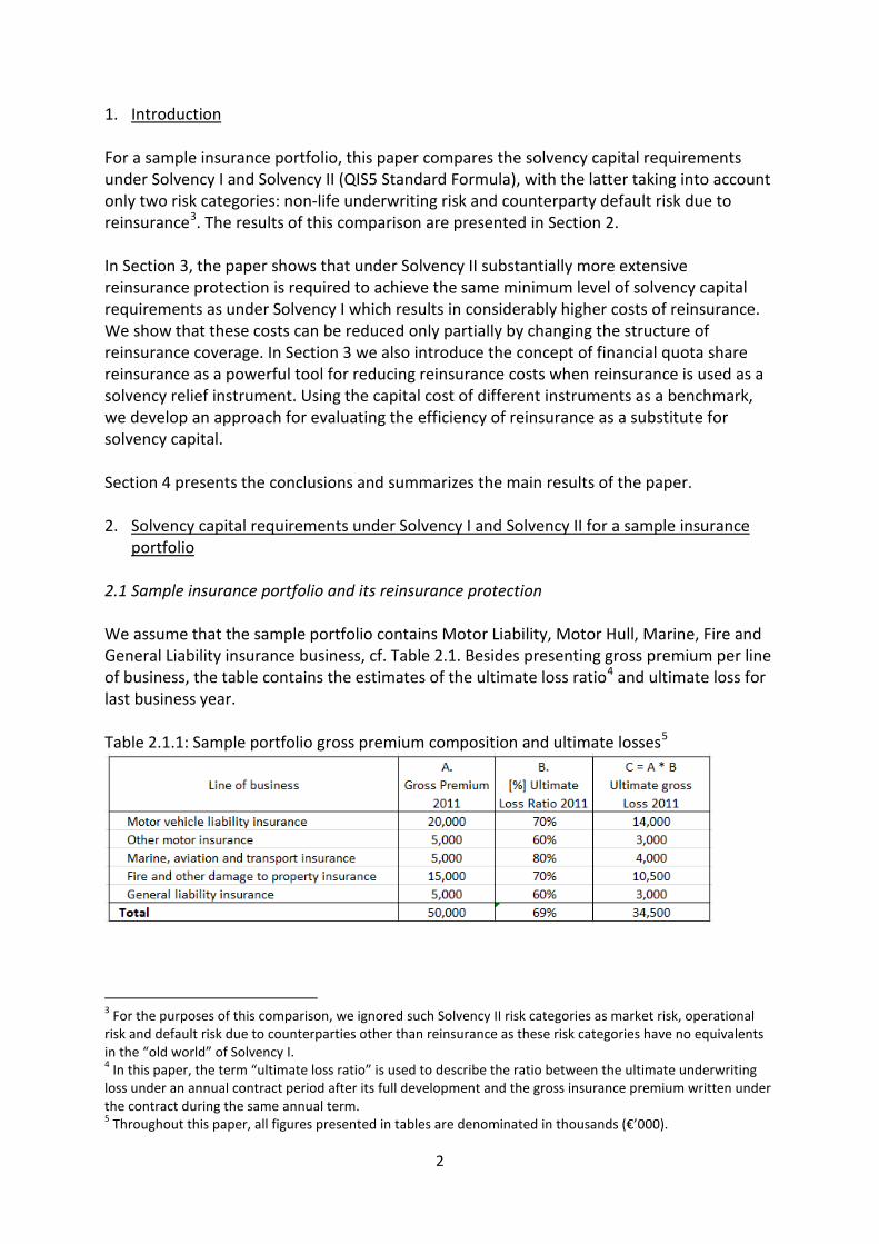
1. Introduction For a sample insurance portfolio, this paper compares the solvency capital requirements under Solvency I and Solvency II (QIS5 Standard Formula), with the latter taking into account only two risk categories: non-life underwriting risk and counterparty default risk due to reinsurance3. The results of this comparison are presented in Section 2. In Section 3, the paper shows that under Solvency II substantially more extensive reinsurance protection is required to achieve the same minimum level of solvency capital requirements as under Solvency I which results in considerably higher costs of reinsurance. We show that these costs can be reduced only partially by changing the structure of reinsurance coverage. In Section 3 we also introduce the concept of financial quota share reinsurance as a powerful tool for reducing reinsurance costs when reinsurance is used as a solvency relief instrument. Using the capital cost of different instruments as a benchmark, we develop an approach for evaluating the efficiency of reinsurance as a substitute for solvency capital. Section 4 presents the conclusions and summarizes the main results of the paper. 2. Solvency capital requirements under Solvency I and Solvency II for a sample insurance

portfolio

2.1 Sample insurance portfolio and its reinsurance protection We assume that the sample portfolio contains Motor Liability, Motor Hull, Marine, Fire and General Liability insurance business, cf. Table 2.1. Besides presenting gross premium per line of business, the table contains the estimates of the ultimate loss ratio4 and ultimate loss for last business year. Table 2.1.1: Sample portfolio gross premium composition and ultimate losses5

3 For the purposes of this comparison, we ignored such Solvency II risk categories as market risk, operational risk and default risk due to counterparties other than reinsurance as these risk categories have no equivalents in the “old world” of Solvency I. 4 In this paper, the term “ultimate loss ratio” is used to describe the ratio between the ultimate underwriting loss under an annual contract period after its full development and the gross insurance premium written under the contract during the same annual term. 5 Throughout this paper, all figures presented in tables are denominated in thousands (€’000).

3

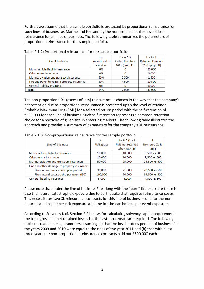
Further, we assume that the sample portfolio is protected by proportional reinsurance for such lines of business as Marine and Fire and by the non-proportional excess of loss reinsurance for all lines of business. The following table summarizes the parameters of proportional reinsurance for the sample portfolio. Table 2.1.2: Proportional reinsurance for the sample portfolio

The non-proportional XL (excess of loss) reinsurance is chosen in the way that the company’s net retention due to proportional reinsurance is protected up to the level of retained Probable Maximum Loss (PML) for a selected return period with the self-retention of €500,000 for each line of business. Such self-retention represents a common retention choice for a portfolio of given size in emerging markets. The following table illustrates the approach and provides a summary of parameters for the company’s XL reinsurance. Table 2.1.3: Non-proportional reinsurance for the sample portfolio

Please note that under the line of business Fire along with the “pure” fire exposure there is also the natural catastrophe exposure due to earthquake that requires reinsurance cover. This necessitates two XL reinsurance contracts for this line of business – one for the non-natural-catastrophe per risk exposure and one for the earthquake per event exposure. According to Solvency I, cf. Section 2.2 below, for calculating solvency capital requirements the total gross and net retained losses for the last three years are required. The following table calculates these parameters assuming (a) that the loss burdens per line of business for the years 2009 and 2010 were equal to the ones of the year 2011 and (b) that within last three years the non-proportional reinsurance contracts paid out €500,000 each.

4

Table 2.1.4: Total gross and net underwriting loss for the last three business years

2.2 Solvency capital requirements for the sample insurance portfolio according to Solvency I6 First, the Retention Ratio needs to be calculated. The following table provides the result for the sample portfolio whereas the figures in columns A and B were taken from the Table 2.1.4, columns K and N. Table 2.2.1: Solvency I, Retention Ratio

Then we can calculate the Premium Index (Table 2.2.2) and the Claims Index (Table 2.2.3) Table 2.2.2: Solvency I, Premium Index (EUR 000)

Adjusted gross premium in column D of Table 2.2.2 is computed as the total gross premium plus 50% of the premium for general liability, cf. Table 2.1.1 and Annex A1. Table 2.2.3: Solvency I, Claims Index (EUR 000)

The adjusted gross loss in column H of Table 2.2.3 is the product of the total gross loss plus 50% of the loss for general liability, cf. Table 2.1.4 and Annex A1.

6 For more details on calculating solvency capital requirements under Solvency I, see Annex A1.

5

The solvency capital requirement according to Solvency I is calculated as the maximum between the Premium Index and Claims Index. For the sample portfolio, we obtain Solvency Capital Requirement = max (Premium Index; Claims Index)

= max (7,765; 7,691)= €7,765

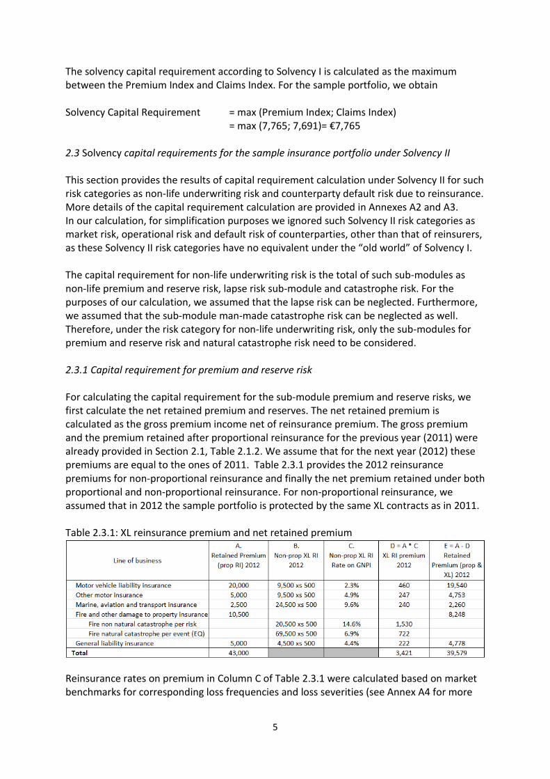
2.3 Solvency capital requirements for the sample insurance portfolio under Solvency II This section provides the results of capital requirement calculation under Solvency II for such risk categories as non-life underwriting risk and counterparty default risk due to reinsurance. More details of the capital requirement calculation are provided in Annexes A2 and A3. In our calculation, for simplification purposes we ignored such Solvency II risk categories as market risk, operational risk and default risk of counterparties, other than that of reinsurers, as these Solvency II risk categories have no equivalent under the “old world” of Solvency I. The capital requirement for non-life underwriting risk is the total of such sub-modules as non-life premium and reserve risk, lapse risk sub-module and catastrophe risk. For the purposes of our calculation, we assumed that the lapse risk can be neglected. Furthermore, we assumed that the sub-module man-made catastrophe risk can be neglected as well. Therefore, under the risk category for non-life underwriting risk, only the sub-modules for premium and reserve risk and natural catastrophe risk need to be considered. 2.3.1 Capital requirement for premium and reserve risk For calculating the capital requirement for the sub-module premium and reserve risks, we first calculate the net retained premium and reserves. The net retained premium is calculated as the gross premium income net of reinsurance premium. The gross premium and the premium retained after proportional reinsurance for the previous year (2011) were already provided in Section 2.1, Table 2.1.2. We assume that for the next year (2012) these premiums are equal to the ones of 2011. Table 2.3.1 provides the 2012 reinsurance premiums for non-proportional reinsurance and finally the net premium retained under both proportional and non-proportional reinsurance. For non-proportional reinsurance, we assumed that in 2012 the sample portfolio is protected by the same XL contracts as in 2011. Table 2.3.1: XL reinsurance premium and net retained premium

Reinsurance rates on premium in Column C of Table 2.3.1 were calculated based on market benchmarks for corresponding loss frequencies and loss severities (see Annex A4 for more

6

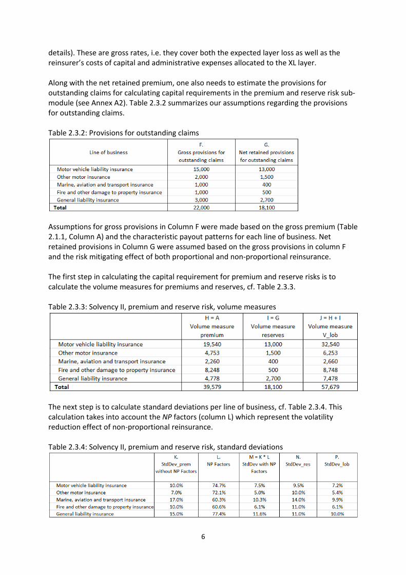
details). These are gross rates, i.e. they cover both the expected layer loss as well as the reinsurer’s costs of capital and administrative expenses allocated to the XL layer. Along with the net retained premium, one also needs to estimate the provisions for outstanding claims for calculating capital requirements in the premium and reserve risk sub-module (see Annex A2). Table 2.3.2 summarizes our assumptions regarding the provisions for outstanding claims. Table 2.3.2: Provisions for outstanding claims

Assumptions for gross provisions in Column F were made based on the gross premium (Table 2.1.1, Column A) and the characteristic payout patterns for each line of business. Net retained provisions in Column G were assumed based on the gross provisions in column F and the risk mitigating effect of both proportional and non-proportional reinsurance. The first step in calculating the capital requirement for premium and reserve risks is to calculate the volume measures for premiums and reserves, cf. Table 2.3.3. Table 2.3.3: Solvency II, premium and reserve risk, volume measures

The next step is to calculate standard deviations per line of business, cf. Table 2.3.4. This calculation takes into account the NP factors (column L) which represent the volatility reduction effect of non-proportional reinsurance. Table 2.3.4: Solvency II, premium and reserve risk, standard deviations

7

Table 2.3.5 completes the calculation. It provides the results for the total volume measure (column Q), total standard deviation (column R), the function 𝜌 of the total standard deviation, which approximates the 99.5% VaR (column S), and finally the capital requirement for non-life premium and the reserve risk (column T). Table 2.3.5: Solvency II, capital requirement for premium and reserve risk

For a detailed explanation of the calculation steps presented in Tables 2.3.3, 2.3.4 and 2.3.5, please refer to Annex A2, section A2.2. 2.3.2 Capital requirement for natural catastrophe risk The only natural catastrophe risk covered by the sample portfolio is the earthquake risk. According to Table 2.1.3, the PML for the earthquake risk is € 100m. We assume that this PML is the 200 years loss. The capital requirement for earthquake risk according to Solvency II is equal to the 200 years loss net of the risk mitigation due to reinsurance. The following Table 2.3.6 summarizes the calculation of risk mitigation and provides the resulting capital requirement. Table 2.3.6 Capital requirement for natural catastrophe risk

For more details on the calculation of capital requirement for natural catastrophe risk, please refer to Annex A2, section A2.4. 2.3.3 Total capital requirement for premium and reserve risk and natural catastrophe risk In this section, we calculate the total capital requirement for premium and reserve risks and the natural catastrophe risk. Capital requirements for these sub-modules taken individually were calculated in sections 2.3.1 and 2.3.2. The total capital requirement results from both individual capital requirements and some diversification effects, cf. Annex A2, section A2.1. Table 2.3.7 provides the resulting capital requirement.

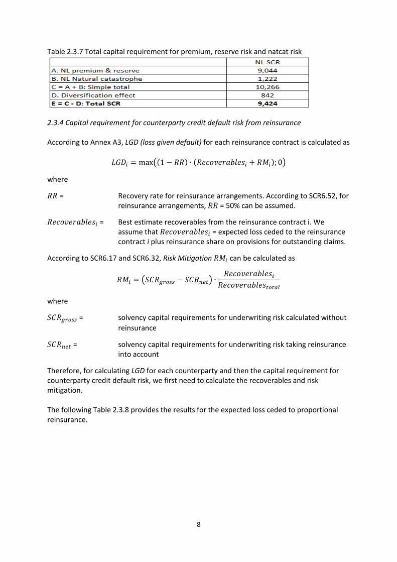
8

Table 2.3.7 Total capital requirement for premium, reserve risk and natcat risk

2.3.4 Capital requirement for counterparty credit default risk from reinsurance According to Annex A3, LGD (loss given default) for each reinsurance contract is calculated as

𝐿𝐺𝐷𝑖 = max�(1 − 𝑅𝑅) ∙ (𝑅𝑒𝑐𝑜𝑣𝑒𝑟𝑎𝑏𝑙𝑒𝑠𝑖 + 𝑅𝑀𝑖); 0�

where

𝑅𝑅 = Recovery rate for reinsurance arrangements. According to SCR6.52, for reinsurance arrangements, 𝑅𝑅 = 50% can be assumed.

𝑅𝑒𝑐𝑜𝑣𝑒𝑟𝑎𝑏𝑙𝑒𝑠𝑖 = Best estimate recoverables from the reinsurance contract i. We assume that 𝑅𝑒𝑐𝑜𝑣𝑒𝑟𝑎𝑏𝑙𝑒𝑠𝑖 = expected loss ceded to the reinsurance contract i plus reinsurance share on provisions for outstanding claims.

According to SCR6.17 and SCR6.32, Risk Mitigation 𝑅𝑀𝑖 can be calculated as

𝑅𝑀𝑖 = �𝑆𝐶𝑅𝑔𝑟𝑜𝑠𝑠 − 𝑆𝐶𝑅𝑛𝑒𝑡� ∙𝑅𝑒𝑐𝑜𝑣𝑒𝑟𝑎𝑏𝑙𝑒𝑠𝑖

𝑅𝑒𝑐𝑜𝑣𝑒𝑟𝑎𝑏𝑙𝑒𝑠𝑡𝑜𝑡𝑎𝑙

where

𝑆𝐶𝑅𝑔𝑟𝑜𝑠𝑠 = solvency capital requirements for underwriting risk calculated without reinsurance

𝑆𝐶𝑅𝑛𝑒𝑡 = solvency capital requirements for underwriting risk taking reinsurance into account

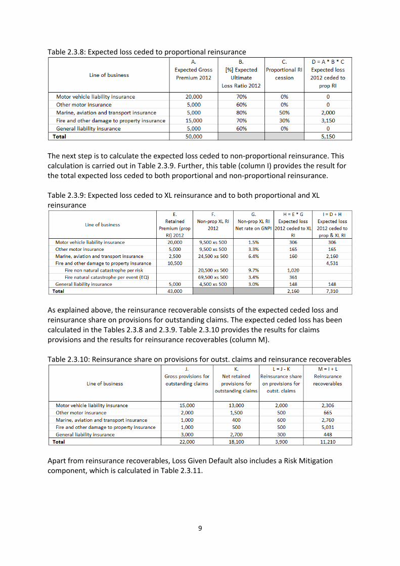
Therefore, for calculating LGD for each counterparty and then the capital requirement for counterparty credit default risk, we first need to calculate the recoverables and risk mitigation. The following Table 2.3.8 provides the results for the expected loss ceded to proportional reinsurance.

9

Table 2.3.8: Expected loss ceded to proportional reinsurance

The next step is to calculate the expected loss ceded to non-proportional reinsurance. This calculation is carried out in Table 2.3.9. Further, this table (column I) provides the result for the total expected loss ceded to both proportional and non-proportional reinsurance. Table 2.3.9: Expected loss ceded to XL reinsurance and to both proportional and XL reinsurance

As explained above, the reinsurance recoverable consists of the expected ceded loss and reinsurance share on provisions for outstanding claims. The expected ceded loss has been calculated in the Tables 2.3.8 and 2.3.9. Table 2.3.10 provides the results for claims provisions and the results for reinsurance recoverables (column M). Table 2.3.10: Reinsurance share on provisions for outst. claims and reinsurance recoverables

Apart from reinsurance recoverables, Loss Given Default also includes a Risk Mitigation component, which is calculated in Table 2.3.11.

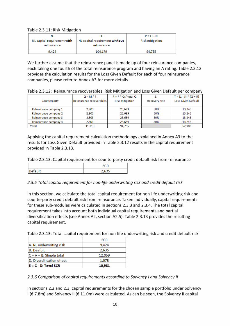
10

Table 2.3.11: Risk Mitigation

We further assume that the reinsurance panel is made up of four reinsurance companies, each taking one fourth of the total reinsurance program and having an A rating. Table 2.3.12 provides the calculation results for the Loss Given Default for each of four reinsurance companies, please refer to Annex A3 for more details. Table 2.3.12: Reinsurance recoverables, Risk Mitigation and Loss Given Default per company

Applying the capital requirement calculation methodology explained in Annex A3 to the results for Loss Given Default provided in Table 2.3.12 results in the capital requirement provided in Table 2.3.13. Table 2.3.13: Capital requirement for counterparty credit default risk from reinsurance

2.3.5 Total capital requirement for non-life underwriting risk and credit default risk In this section, we calculate the total capital requirement for non-life underwriting risk and counterparty credit default risk from reinsurance. Taken individually, capital requirements for these sub-modules were calculated in sections 2.3.3 and 2.3.4. The total capital requirement takes into account both individual capital requirements and partial diversification effects (see Annex A2, section A2.5). Table 2.3.13 provides the resulting capital requirement. Table 2.3.13: Total capital requirement for non-life underwriting risk and credit default risk

2.3.6 Comparison of capital requirements according to Solvency I and Solvency II In sections 2.2 and 2.3, capital requirements for the chosen sample portfolio under Solvency I (€ 7.8m) and Solvency II (€ 11.0m) were calculated. As can be seen, the Solvency II capital

11

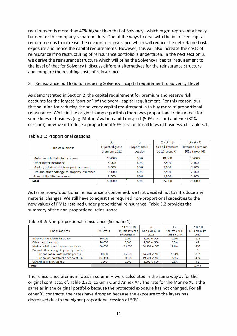
requirement is more than 40% higher than that of Solvency I which might represent a heavy burden for the company’s shareholders. One of the ways to deal with the increased capital requirement is to increase the cession to reinsurance which will reduce the net retained risk exposure and hence the capital requirements. However, this will also increase the costs of reinsurance if no restructuring of reinsurance portfolio is undertaken. In the next section 3, we derive the reinsurance structure which will bring the Solvency II capital requirement to the level of that for Solvency I, discuss different alternatives for the reinsurance structure and compare the resulting costs of reinsurance. 3. Reinsurance portfolio for reducing Solvency II capital requirement to Solvency I level As demonstrated in Section 2, the capital requirement for premium and reserve risk accounts for the largest “portion” of the overall capital requirement. For this reason, our first solution for reducing the solvency capital requirement is to buy more of proportional reinsurance. While in the original sample portfolio there was proportional reinsurance for some lines of business (e.g. Motor, Aviation and Transport (50% cession) and Fire (30% cession)), now we introduce a proportional 50% cession for all lines of business, cf. Table 3.1. Table 3.1: Proportional cessions

As far as non-proportional reinsurance is concerned, we first decided not to introduce any material changes. We still have to adjust the required non-proportional capacities to the new values of PMLs retained under proportional reinsurance. Table 3.2 provides the summary of the non-proportional reinsurance. Table 3.2: Non-proportional reinsurance (Scenario 1)

The reinsurance premium rates in column H were calculated in the same way as for the original contracts, cf. Table 2.3.1, column C and Annex A4. The rate for the Marine XL is the same as in the original portfolio because the protected exposure has not changed. For all other XL contracts, the rates have dropped because the exposure to the layers has decreased due to the higher proportional cession of 50%.

12

Table 3.3 provides the solvency capital requirement which results from the above reinsurance structure defined by Table 3.1 and Table 3.2. Table 3.3: Total capital requirement for non-life underwriting risk and credit default risk

As we see, we have achieved a substantial reduction of solvency capital requirement compared to the original portfolio (Table 2.3.13), however the level of Solvency I (€ 7.8m) has not yet been achieved. Now, we will adjust the non-proportional reinsurance and see what effect on the capital requirement such an adjustment will have. We will reduce the retentions of non-proportional contract to a € 250k. The following Table 3.4 summarizes the new non-proportional reinsurance portfolio. Table 3.4: Non-proportional reinsurance (Variant 2)

Pricing rates in column H were calculated in the same way as for the original contracts, cf. Table 2.3.1, column C and Table 3.2, column H and Annex A4. With these adjusted non-proportional reinsurance contracts, the resulting capital requirement is as per Table 3.5. Table 3.5: Total capital requirement for non-life underwriting risk and credit default risk (Scenario 2)

One can see that although the resulting capital requirement is getting closer to the one of Solvency I, it is still above it by about € 1.1m. The comparison of Table 3.3 and Table 3.5 shows that the capital requirement for the underwriting risk has dropped while the capital requirement for the counterparty default risk has increased. Both movements can be explained by the more extensive XL reinsurance covers in Scenario 2 - the net retained

13

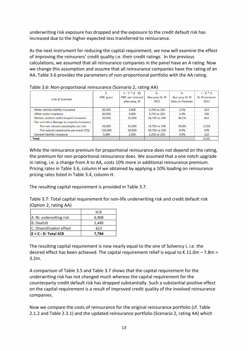
underwriting risk exposure has dropped and the exposure to the credit default risk has increased due to the higher expected loss transferred to reinsurance. As the next instrument for reducing the capital requirement, we now will examine the effect of improving the reinsurers’ credit quality i.e. their credit ratings. In the previous calculations, we assumed that all reinsurance companies in the panel have an A rating. Now we change this assumption and assume that all reinsurance companies have the rating of an AA. Table 3.6 provides the parameters of non-proportional portfolio with the AA rating. Table 3.6: Non-proportional reinsurance (Scenario 2, rating AA)

While the reinsurance premium for proportional reinsurance does not depend on the rating, the premium for non-proportional reinsurance does. We assumed that a one notch upgrade in rating, i.e. a change from A to AA, costs 10% more in additional reinsurance premium. Pricing rates in Table 3.6, column H we obtained by applying a 10% loading on reinsurance pricing rates listed in Table 3.4, column H. The resulting capital requirement is provided in Table 3.7. Table 3.7: Total capital requirement for non-life underwriting risk and credit default risk (Option 2, rating AA)

The resulting capital requirement is now nearly equal to the one of Solvency I, i.e. the desired effect has been achieved. The capital requirement relief is equal to € 11.0m – 7.8m = 3.2m. A comparison of Table 3.5 and Table 3.7 shows that the capital requirement for the underwriting risk has not changed much whereas the capital requirement for the counterparty credit default risk has dropped substantially. Such a substantial positive effect on the capital requirement is a result of improved credit quality of the involved reinsurance companies. Now we compare the costs of reinsurance for the original reinsurance portfolio (cf. Table 2.1.2 and Table 2.3.1) and the updated reinsurance portfolio (Scenario 2, rating AA) which

14

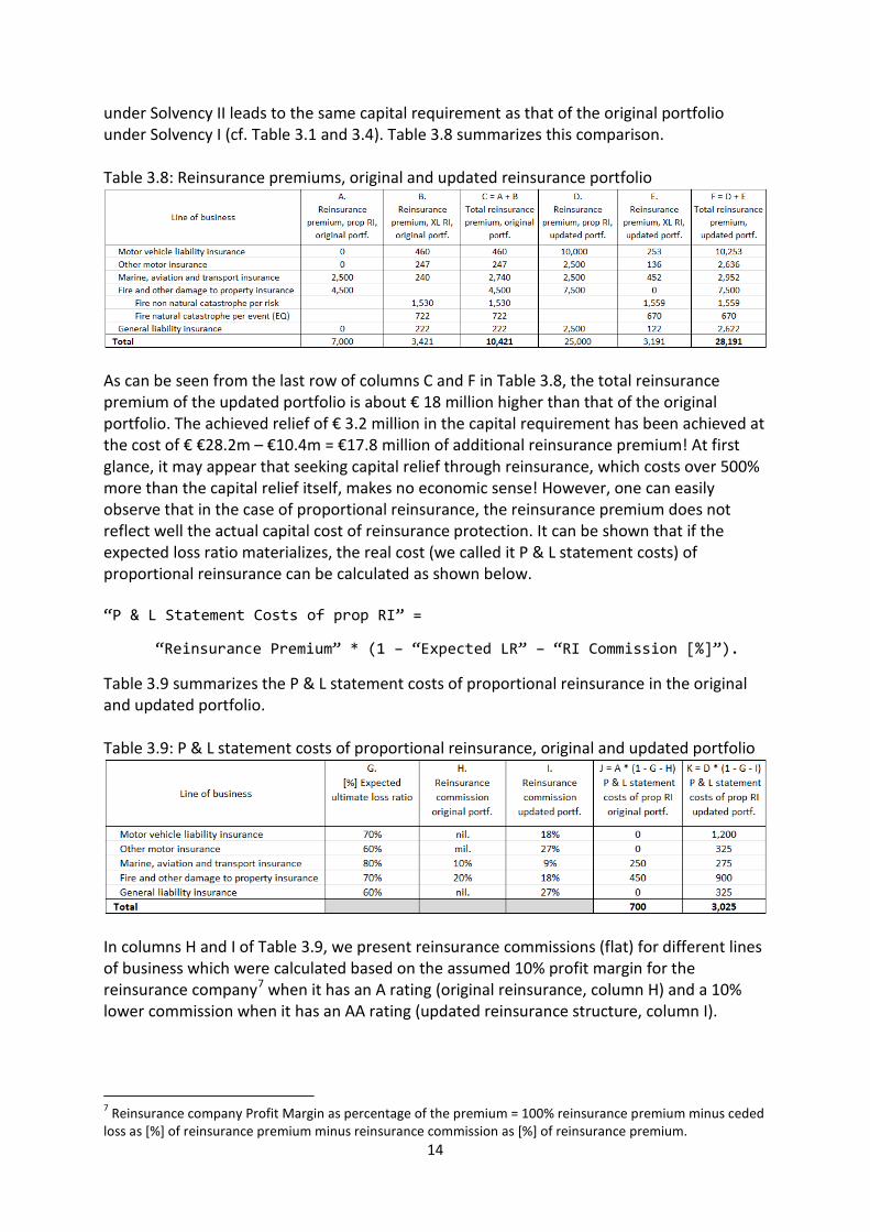
under Solvency II leads to the same capital requirement as that of the original portfolio under Solvency I (cf. Table 3.1 and 3.4). Table 3.8 summarizes this comparison. Table 3.8: Reinsurance premiums, original and updated reinsurance portfolio

As can be seen from the last row of columns C and F in Table 3.8, the total reinsurance premium of the updated portfolio is about € 18 million higher than that of the original portfolio. The achieved relief of € 3.2 million in the capital requirement has been achieved at the cost of € €28.2m – €10.4m = €17.8 million of additional reinsurance premium! At first glance, it may appear that seeking capital relief through reinsurance, which costs over 500% more than the capital relief itself, makes no economic sense! However, one can easily observe that in the case of proportional reinsurance, the reinsurance premium does not reflect well the actual capital cost of reinsurance protection. It can be shown that if the expected loss ratio materializes, the real cost (we called it P & L statement costs) of proportional reinsurance can be calculated as shown below. “P & L Statement Costs of prop RI” =

“Reinsurance Premium” * (1 – “Expected LR” – “RI Commission [%]”).

Table 3.9 summarizes the P & L statement costs of proportional reinsurance in the original and updated portfolio. Table 3.9: P & L statement costs of proportional reinsurance, original and updated portfolio

In columns H and I of Table 3.9, we present reinsurance commissions (flat) for different lines of business which were calculated based on the assumed 10% profit margin for the reinsurance company7 when it has an A rating (original reinsurance, column H) and a 10% lower commission when it has an AA rating (updated reinsurance structure, column I).

7 Reinsurance company Profit Margin as percentage of the premium = 100% reinsurance premium minus ceded loss as [%] of reinsurance premium minus reinsurance commission as [%] of reinsurance premium.

15

Now we can compare the overall costs of the original and updated reinsurance portfolio made of reinsurance premium for non-proportional XL reinsurance and P & L statement costs of proportional reinsurance, cf. Table 3.10. Table 3.10: total P & L statement costs of reinsurance, original and updated portfolio

Based on the P & L statement costs of reinsurance, the additional costs for the updated reinsurance structure calculates to € 6.2m – 4.1m = 2.1m – the amount which no longer exceeds the achieved € 3.2 million relief in capital requirement. To evaluate the efficiency of reinsurance as the solvency capital relief instrument, we now introduce the relative costs of capital ratio which is calculated as the cost of reinsurance divided by the achieved capital relief. Obviously, the lower this ratio, the better the efficiency of the given reinsurance structure as the capital relief instrument. Furthermore, the straight forward cost of capital approach afforded by this ratio also allows a direct comparison of reinsurance as a capital relief instrument with capital borrowed from the capital markets. That is if the rates offered by the capital markets are higher than the relative cost of capital ratio resulting for a prospected reinsurance structure, then a given reinsurance structure has a cost advantage over debt instruments as a solvency capital relief instrument. In our case, we calculate the relative cost of capital 2.1m / 3.2m = 65.6% (cost of capital relief divided by the capital relief) which clearly is very high. Most likely, the insurance company would be able to borrow from the capital markets at a much lower rate. To increase the attractiveness of reinsurance as a solvency capital relief instrument compared to borrowing, the cost of reinsurance protection should be reduced substantially. One conventional way to reduce the costs of reinsurance protection is to replace conventional proportional contracts with flat reinsurance commissions with the so called financial quota share (FQS) contracts – a type of proportional contracts which usually has a broad sliding scale reinsurance commission that depends on the underwriting performance of the contract. Such contracts are called financial because along with the transfer of insurance risk they are usually motivated also by financing objectives such as achieving a solvency capital relief. The diagram below provides an example of a sliding scale reinsurance commission. In the loss ratio range of 45%-85% the reinsurance commission is chosen in the way that the total of the loss ratio and commission is kept constant at 95%. Obviously, the resulting reinsurer’s margin in this broad loss ratio range is 5%.

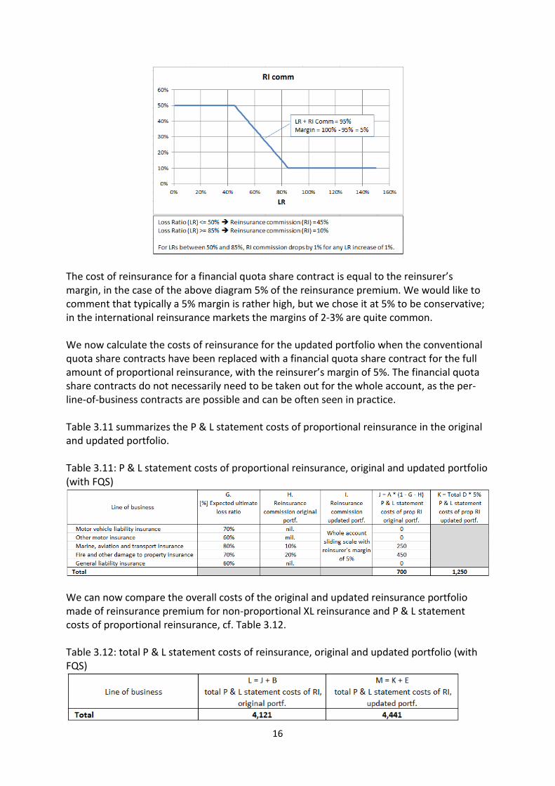
16

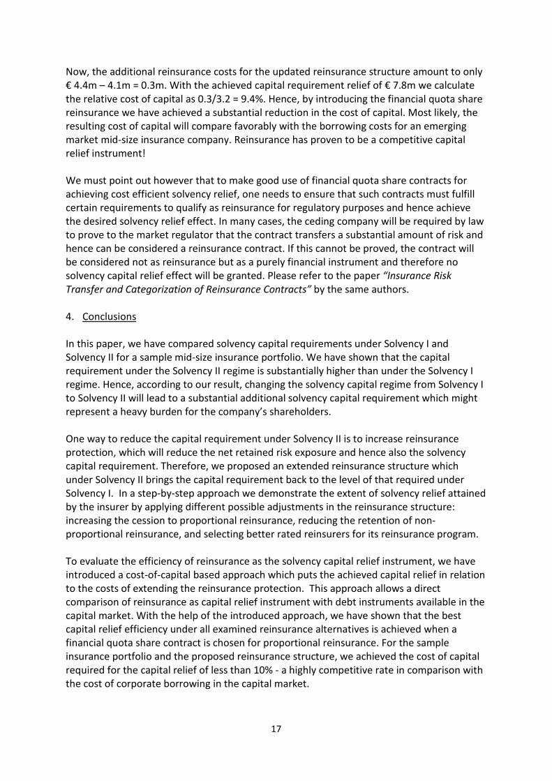
The cost of reinsurance for a financial quota share contract is equal to the reinsurer’s margin, in the case of the above diagram 5% of the reinsurance premium. We would like to comment that typically a 5% margin is rather high, but we chose it at 5% to be conservative; in the international reinsurance markets the margins of 2-3% are quite common. We now calculate the costs of reinsurance for the updated portfolio when the conventional quota share contracts have been replaced with a financial quota share contract for the full amount of proportional reinsurance, with the reinsurer’s margin of 5%. The financial quota share contracts do not necessarily need to be taken out for the whole account, as the per-line-of-business contracts are possible and can be often seen in practice. Table 3.11 summarizes the P & L statement costs of proportional reinsurance in the original and updated portfolio. Table 3.11: P & L statement costs of proportional reinsurance, original and updated portfolio (with FQS)

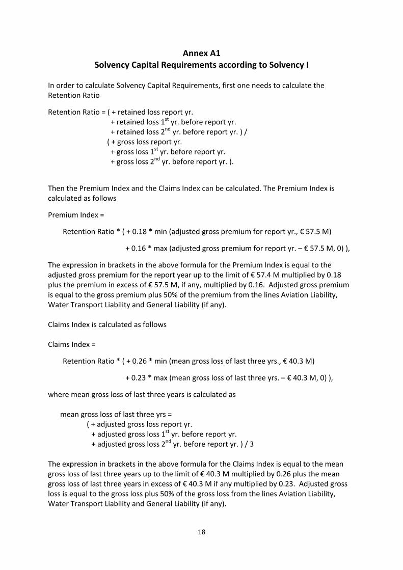
We can now compare the overall costs of the original and updated reinsurance portfolio made of reinsurance premium for non-proportional XL reinsurance and P & L statement costs of proportional reinsurance, cf. Table 3.12. Table 3.12: total P & L statement costs of reinsurance, original and updated portfolio (with FQS)

17

Now, the additional reinsurance costs for the updated reinsurance structure amount to only € 4.4m – 4.1m = 0.3m. With the achieved capital requirement relief of € 7.8m we calculate the relative cost of capital as 0.3/3.2 = 9.4%. Hence, by introducing the financial quota share reinsurance we have achieved a substantial reduction in the cost of capital. Most likely, the resulting cost of capital will compare favorably with the borrowing costs for an emerging market mid-size insurance company. Reinsurance has proven to be a competitive capital relief instrument! We must point out however that to make good use of financial quota share contracts for achieving cost efficient solvency relief, one needs to ensure that such contracts must fulfill certain requirements to qualify as reinsurance for regulatory purposes and hence achieve the desired solvency relief effect. In many cases, the ceding company will be required by law to prove to the market regulator that the contract transfers a substantial amount of risk and hence can be considered a reinsurance contract. If this cannot be proved, the contract will be considered not as reinsurance but as a purely financial instrument and therefore no solvency capital relief effect will be granted. Please refer to the paper “Insurance Risk Transfer and Categorization of Reinsurance Contracts” by the same authors. 4. Conclusions In this paper, we have compared solvency capital requirements under Solvency I and Solvency II for a sample mid-size insurance portfolio. We have shown that the capital requirement under the Solvency II regime is substantially higher than under the Solvency I regime. Hence, according to our result, changing the solvency capital regime from Solvency I to Solvency II will lead to a substantial additional solvency capital requirement which might represent a heavy burden for the company’s shareholders. One way to reduce the capital requirement under Solvency II is to increase reinsurance protection, which will reduce the net retained risk exposure and hence also the solvency capital requirement. Therefore, we proposed an extended reinsurance structure which under Solvency II brings the capital requirement back to the level of that required under Solvency I. In a step-by-step approach we demonstrate the extent of solvency relief attained by the insurer by applying different possible adjustments in the reinsurance structure: increasing the cession to proportional reinsurance, reducing the retention of non-proportional reinsurance, and selecting better rated reinsurers for its reinsurance program. To evaluate the efficiency of reinsurance as the solvency capital relief instrument, we have introduced a cost-of-capital based approach which puts the achieved capital relief in relation to the costs of extending the reinsurance protection. This approach allows a direct comparison of reinsurance as capital relief instrument with debt instruments available in the capital market. With the help of the introduced approach, we have shown that the best capital relief efficiency under all examined reinsurance alternatives is achieved when a financial quota share contract is chosen for proportional reinsurance. For the sample insurance portfolio and the proposed reinsurance structure, we achieved the cost of capital required for the capital relief of less than 10% - a highly competitive rate in comparison with the cost of corporate borrowing in the capital market.

18

Annex A1 Solvency Capital Requirements according to Solvency I

In order to calculate Solvency Capital Requirements, first one needs to calculate the Retention Ratio

Retention Ratio = ( + retained loss report yr. + retained loss 1st yr. before report yr.

+ retained loss 2nd yr. before report yr. ) / ( + gross loss report yr.

+ gross loss 1st yr. before report yr. + gross loss 2nd yr. before report yr. ).

Then the Premium Index and the Claims Index can be calculated. The Premium Index is calculated as follows

Premium Index =

Retention Ratio * ( + 0.18 * min (adjusted gross premium for report yr., € 57.5 M)

+ 0.16 * max (adjusted gross premium for report yr. – € 57.5 M, 0) ),

The expression in brackets in the above formula for the Premium Index is equal to the adjusted gross premium for the report year up to the limit of € 57.4 M multiplied by 0.18 plus the premium in excess of € 57.5 M, if any, multiplied by 0.16. Adjusted gross premium is equal to the gross premium plus 50% of the premium from the lines Aviation Liability, Water Transport Liability and General Liability (if any). Claims Index is calculated as follows Claims Index =

Retention Ratio * ( + 0.26 * min (mean gross loss of last three yrs., € 40.3 M)

+ 0.23 * max (mean gross loss of last three yrs. – € 40.3 M, 0) ),

where mean gross loss of last three years is calculated as mean gross loss of last three yrs = ( + adjusted gross loss report yr. + adjusted gross loss 1st yr. before report yr. + adjusted gross loss 2nd yr. before report yr. ) / 3

The expression in brackets in the above formula for the Claims Index is equal to the mean gross loss of last three years up to the limit of € 40.3 M multiplied by 0.26 plus the mean gross loss of last three years in excess of € 40.3 M if any multiplied by 0.23. Adjusted gross loss is equal to the gross loss plus 50% of the gross loss from the lines Aviation Liability, Water Transport Liability and General Liability (if any).

19

Finally, the Solvency Capital Requirement is calculated as maximum of both Premium Index and Claims Index Solvency Capital Requirement = max (Premium Index, Claims Index) If the resulting Solvency Capital Requirement for the report year is lower than for the previous year, the following further calculation needs to be carried out. Loss reserve ratio = max (1, loss reserves at the end of report yr. / loss reserves at the beginning of report yr.) Solvency Capital Requirement = max (max (Premium Index, Claims Index), Loss reserve ratio * Solvency Capital Requirement previous yr.)

20

Annex A2 Solvency Capital Requirements for non-life underwriting risk under Solvency

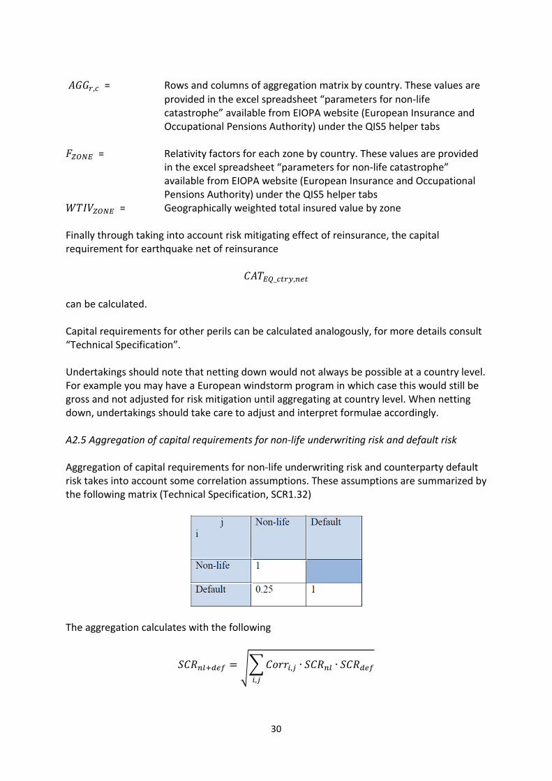
II (QIS5) standard formula This Annex describes the calculation of solvency capital requirements for non-life underwriting risk according to Solvency II (QIS5) standard formula, as defined by EU document “QIS5 Technical Specification” (Brussels, July 2010). The Annex is organized as follows. Section A2.1 describes the overall approach for calculating the solvency capital requirement for non-life underwriting risk based on the results of three sub-modules: non-life premium and reserve risk, non-life lapse risk and non-life catastrophe risk sub-module. Sections A2.2 and A2.4 then provide a detailed explanation of the capital requirement calculation for the sub-modules non-life premium and reserve risk (Section A2.3) and non-life catastrophe risk (Section A2.4). Section A2.3 provides an explanation on the objective and motivation behind the non-life lapse risk sub-module However, the section provides no calculation details as we assume this risk category does not materialize for the sample portfolio under consideration. Finally Section A2.4 explains the aggregation of the capital requirements for the non-life underwriting risk module and the counterparty default risk module (cf. Annex 3). This aggregation takes into account some correlation assumptions between these two risk categories. A2.1 Calculation of the overall capital requirement for non-life underwriting risk The non-life underwriting risk module consists of the following sub-modules:

• The non-life premium and reserve risk sub-module • The non-life lapse risk sub-module • The non-life catastrophe risk sub-module

Capital requirements for each module are denoted by 𝑁𝐿𝑝𝑟 = Capital requirement for non-life premium and reserve risk 𝑁𝐿𝑙𝑎𝑝𝑠𝑒 = Capital requirement for non-life lapse risk 𝑁𝐿𝐶𝐴𝑇 = Capital requirement for non-life catastrophe risk The resulting solvency Capital requirement for non-life underwriting risk is denoted by 𝑆𝐶𝑅𝑛𝑙 = Capital requirement for non-life underwriting risk It calculates by combining the capital requirements for the non-life sub-risks using a correlation matrix as follows

𝑆𝐶𝑅𝑛𝑙 = ��𝐶𝑜𝑟𝑟𝑁𝐿𝑟,𝑐 ∙ 𝑁𝐿𝑟 ∙ 𝑁𝐿𝑐

where 𝐶𝑜𝑟𝑟𝑁𝐿𝑟,𝑐 = The entries of the correlation matrix 𝐶𝑜𝑟𝑟𝑁𝐿

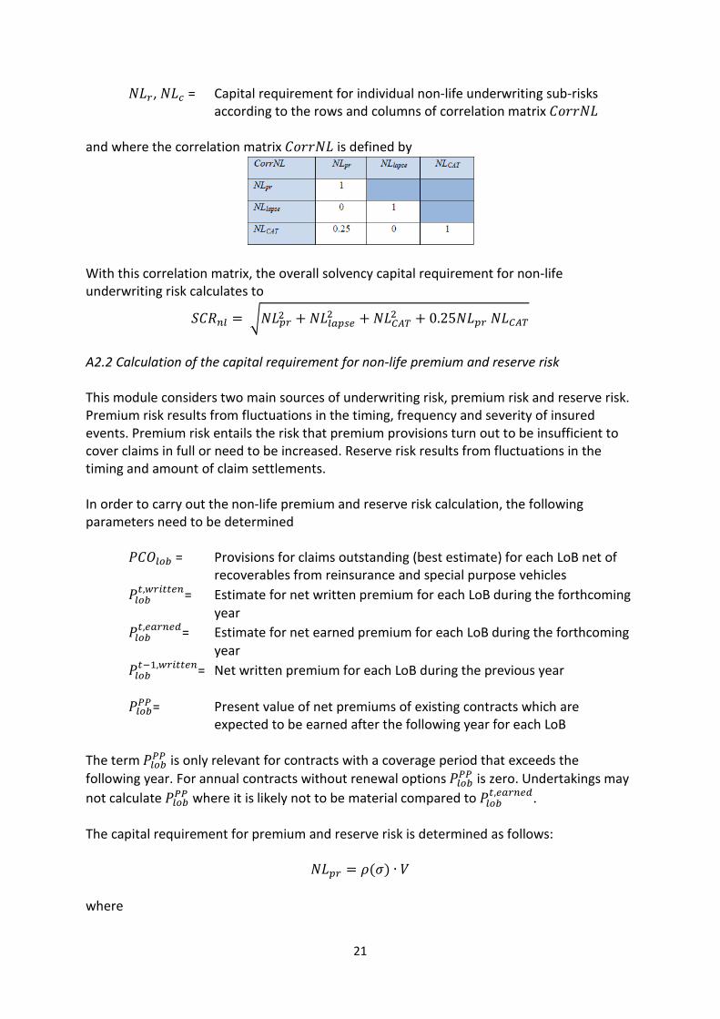
21

𝑁𝐿𝑟, 𝑁𝐿𝑐 = Capital requirement for individual non-life underwriting sub-risks according to the rows and columns of correlation matrix 𝐶𝑜𝑟𝑟𝑁𝐿

and where the correlation matrix 𝐶𝑜𝑟𝑟𝑁𝐿 is defined by

With this correlation matrix, the overall solvency capital requirement for non-life underwriting risk calculates to

𝑆𝐶𝑅𝑛𝑙 = �𝑁𝐿𝑝𝑟2 + 𝑁𝐿𝑙𝑎𝑝𝑠𝑒2 + 𝑁𝐿𝐶𝐴𝑇2 + 0.25𝑁𝐿𝑝𝑟 𝑁𝐿𝐶𝐴𝑇

A2.2 Calculation of the capital requirement for non-life premium and reserve risk This module considers two main sources of underwriting risk, premium risk and reserve risk. Premium risk results from fluctuations in the timing, frequency and severity of insured events. Premium risk entails the risk that premium provisions turn out to be insufficient to cover claims in full or need to be increased. Reserve risk results from fluctuations in the timing and amount of claim settlements. In order to carry out the non-life premium and reserve risk calculation, the following parameters need to be determined

𝑃𝐶𝑂𝑙𝑜𝑏 = Provisions for claims outstanding (best estimate) for each LoB net of recoverables from reinsurance and special purpose vehicles

𝑃𝑙𝑜𝑏𝑡,𝑤𝑟𝑖𝑡𝑡𝑒𝑛= Estimate for net written premium for each LoB during the forthcoming

year 𝑃𝑙𝑜𝑏𝑡,𝑒𝑎𝑟𝑛𝑒𝑑= Estimate for net earned premium for each LoB during the forthcoming

year 𝑃𝑙𝑜𝑏𝑡−1,𝑤𝑟𝑖𝑡𝑡𝑒𝑛= Net written premium for each LoB during the previous year

𝑃𝑙𝑜𝑏𝑃𝑃= Present value of net premiums of existing contracts which are

expected to be earned after the following year for each LoB The term 𝑃𝑙𝑜𝑏𝑃𝑃 is only relevant for contracts with a coverage period that exceeds the following year. For annual contracts without renewal options 𝑃𝑙𝑜𝑏𝑃𝑃 is zero. Undertakings may not calculate 𝑃𝑙𝑜𝑏𝑃𝑃 where it is likely not to be material compared to 𝑃𝑙𝑜𝑏

𝑡,𝑒𝑎𝑟𝑛𝑒𝑑. The capital requirement for premium and reserve risk is determined as follows:

𝑁𝐿𝑝𝑟 = 𝜌(𝜎) ∙ 𝑉

where

22

𝑉 = Volume measure 𝜎 = Combined standard deviation 𝜌(𝜎) = A function of the combined standard deviation

The function 𝜌(𝜎) is specified as follows:

𝜌(𝜎) = exp (𝑁0.995 ∙ �log (𝜎2 + 1))

√𝜎2 + 1 − 1

where

𝑁0.995 = 99.5% quantile of the standard normal distribution (≈2.576) The function 𝜌(𝜎) is set in such a way that, assuming a lognormal distribution of the underlying risk, a risk capital requirement consistent with the VaR 99.5% calibration objective is produced. Roughly, 𝜌(𝜎) ≈ 3 ∙ 𝜎. The volume measure V and the combined standard deviation σ for the overall non-life insurance portfolio are determined in two steps as follows:

• For each individual LoB, the standard deviations and volume measures for both premium risk and reserve risk are determined;

• The standard deviations and volume measures for the premium risk and the reserve risk in the individual LoBs are aggregated to derive an overall volume measure V and a combined standard deviation σ.

The calculations needed to perform these two steps are set out below. Step 1: Volume measures and standard deviations per LoB The following numbering of LoBs applies for the calculation:

For each LoB, the volume measures and standard deviations for premium and reserve risk are denoted as follows:

23

𝑉(𝑝𝑟𝑒𝑚,𝑙𝑜𝑏) = The volume measure for premium risk 𝑉(𝑟𝑒𝑠,𝑙𝑜𝑏) = The volume measure for reserve risk 𝜎(𝑝𝑟𝑒𝑚,𝑙𝑜𝑏) = Standard deviation for premium risk 𝜎(𝑟𝑒𝑠,𝑙𝑜𝑏) = Standard deviation for reserve risk

The volume measure for premium risk in the individual LoB is determined as follows:

𝑉(𝑝𝑟𝑒𝑚,𝑙𝑜𝑏) = max�𝑃𝑙𝑜𝑏𝑡,𝑤𝑟𝑖𝑡𝑡𝑒𝑛; 𝑃𝑙𝑜𝑏

𝑡,𝑒𝑎𝑟𝑛𝑒𝑑; 𝑃𝑙𝑜𝑏𝑡−1,𝑤𝑟𝑖𝑡𝑡𝑒𝑛� + 𝑃𝑙𝑜𝑏𝑃𝑃

If the undertaking has committed to its regulator that it will restrict premiums written over the period so that the actual premiums written (or earned) over the period will not exceed its estimated volumes, the volume measure is determined only with respect to estimated premium volumes, so that in this case:

𝑉(𝑝𝑟𝑒𝑚,𝑙𝑜𝑏) = max�𝑃𝑙𝑜𝑏𝑡,𝑤𝑟𝑖𝑡𝑡𝑒𝑛; 𝑃𝑙𝑜𝑏

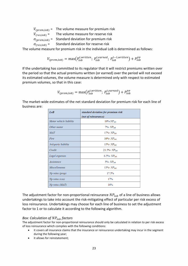
𝑡,𝑒𝑎𝑟𝑛𝑒𝑑� + 𝑃𝑙𝑜𝑏𝑃𝑃 The market-wide estimates of the net standard deviation for premium risk for each line of business are:

The adjustment factor for non-proportional reinsurance 𝑁𝑃𝑙𝑜𝑏 of a line of business allows undertakings to take into account the risk-mitigating effect of particular per risk excess of loss reinsurance. Undertakings may choose for each line of business to set the adjustment factor to 1 or to calculate it according to the following algorithm. Box: Calculation of 𝑁𝑃𝑙𝑜𝑏 factors The adjustment factor for non-proportional reinsurance should only be calculated in relation to per risk excess of loss reinsurance which complies with the following conditions:

• it covers all insurance claims that the insurance or reinsurance undertaking may incur in the segment during the following year;

• it allows for reinstatement;

24

• it meets the requirements for risk mitigation techniques, set out in subsection SCR.13 of the defined by EU document “QIS5 Technical Specification” (Brussels, July 2010).

𝑁𝑃𝑙𝑜𝑏 = �1 + (Ω𝑙𝑜𝑏𝑛𝑒𝑡 ∕ 𝑀𝑙𝑜𝑏

𝑛𝑒𝑡)2

1 + (Ω𝑙𝑜𝑏𝑔𝑟𝑜𝑠𝑠 ∕ 𝑀𝑙𝑜𝑏

𝑔𝑟𝑜𝑠𝑠)2

where 𝑀𝑙𝑜𝑏

𝑛𝑒𝑡 = 𝑀𝑙𝑜𝑏𝑔𝑟𝑜𝑠𝑠 ⋅ �1 − 𝐹𝑚+𝜎2,𝜎(𝑎 + 𝑏) + 𝐹𝑚+𝜎2,𝜎(𝑎)� + 𝑎 ∙ �𝐹𝑚,𝜎(𝑎 + 𝑏) − 𝐹𝑚,𝜎(𝑎)� − 𝑏 ∙ �1 − 𝐹𝑚,𝜎(𝑎 + 𝑏)�

Ω𝑙𝑜𝑏𝑛𝑒𝑡 = ���Ω𝑙𝑜𝑏𝑔𝑟𝑜𝑠𝑠�2 + �𝑀𝑙𝑜𝑏

𝑔𝑟𝑜𝑠𝑠�2� ∙ �1 − 𝐹𝑚+2𝜎2,𝜎(𝑎 + 𝑏) + 𝐹𝑚+2𝜎2,𝜎(𝑎)� + 𝑎2 ∙ �𝐹𝑚,𝜎(𝑎 + 𝑏) − 𝐹𝑚,𝜎(𝑎)�

− 2𝑏 ∙ 𝑀𝑙𝑜𝑏𝑔𝑟𝑜𝑠𝑠 ∙ �1 − 𝐹𝑚+𝜎2,𝜎(𝑎 + 𝑏)� + 𝑏2 ∙ �1 − 𝐹𝑚,𝜎(𝑎 + 𝑏)� − (𝑀𝑙𝑜𝑏

𝑛𝑒𝑡)2�1/2

𝜎 = �ln�1 + �Ω𝑙𝑜𝑏𝑔𝑟𝑜𝑠𝑠

𝑀𝑙𝑜𝑏𝑔𝑟𝑜𝑠𝑠�

2

�

𝑚 = ln𝑀𝑙𝑜𝑏𝑔𝑟𝑜𝑠𝑠 −

𝜎2

2

𝑀𝑙𝑜𝑏𝑔𝑟𝑜𝑠𝑠 = �

𝑀�𝑙𝑜𝑏𝑔𝑟𝑜𝑠𝑠 if 𝑆 ≥ 1

𝑆 ∙ 𝑀�𝑙𝑜𝑏𝑔𝑟𝑜𝑠𝑠 otherwise

Ω𝑙𝑜𝑏𝑔𝑟𝑜𝑠𝑠 = �

Ω�𝑙𝑜𝑏𝑔𝑟𝑜𝑠𝑠 if 𝑆 ≥ 1

𝑆 ∙ Ω�𝑙𝑜𝑏𝑔𝑟𝑜𝑠𝑠 otherwise

𝑆 = �𝑛 ∙ 𝜎(𝑝𝑟𝑒𝑚,𝑔𝑟𝑜𝑠𝑠,𝑙𝑜𝑏)

2 ∙ 𝑉(𝑝𝑟𝑒𝑚,𝑔𝑟𝑜𝑠𝑠,𝑙𝑜𝑏)2

𝑁 ∙ ��Ω�𝑙𝑜𝑏𝑔𝑟𝑜𝑠𝑠�2 + �𝑀�𝑙𝑜𝑏

𝑔𝑟𝑜𝑠𝑠�2�

The terms used in these formulas are defined as follows

𝑀�𝑙𝑜𝑏

𝑔𝑟𝑜𝑠𝑠 = Average cost per claim gross of reinsurance per LoB estimated from the claims of the last 𝑛 years where 𝑛 ≥ 1

Ω�𝑙𝑜𝑏𝑔𝑟𝑜𝑠𝑠 = Standard deviation of the cost per claim gross of reinsurance per LoB estimated with

the standard estimator from the claims of the last 𝑛 years where 𝑛 ≥ 1 𝑎 = Retention of non-proportional reinsurance contract 𝑏 = Limit of non-proportional reinsurance contract 𝐹𝑚,𝜎 = Distribution function of a Lognormal random variable with parameters (𝑚,𝜎) 𝐹𝑚+𝜎2,𝜎 = Distribution function of a Lognormal random variable with parameters (𝑚 + 𝜎2,𝜎) 𝐹𝑚+2𝜎2,𝜎 = Distribution function of a Lognormal random variable with parameters (𝑚 + 2𝜎2,𝜎) 𝑛 = Number of years used in the estimation of 𝑀�𝑙𝑜𝑏

𝑔𝑟𝑜𝑠𝑠 and Ω�𝑙𝑜𝑏𝑔𝑟𝑜𝑠𝑠

𝑁 = Number of claims during the last 𝑛 years

25

𝜎(𝑝𝑟𝑒𝑚,𝑔𝑟𝑜𝑠𝑠,𝑙𝑜𝑏) = Standard deviation for premium risk gross of reinsurance, calculated by putting the adjustment factor 𝑁𝑃𝑙𝑜𝑏 to 1.

𝑉(𝑝𝑟𝑒𝑚,𝑔𝑟𝑜𝑠𝑠,𝑙𝑜𝑏) = Volume measure for premium risk gross of reinsurance, calculated in the

same way as the usual volume measure but based on gross premiums instead of net premiums

Where the excess of loss reinsurance contract has no limit the adjustment factor for non-proportional reinsurance of a line of business shall be calculated in the same way as set out above, but with the following changes: 𝑀𝑙𝑜𝑏

𝑛𝑒𝑡 = 𝑀𝑙𝑜𝑏𝑔𝑟𝑜𝑠𝑠 ⋅ 𝐹𝑚+𝜎2,𝜎(𝑎) + 𝑎 ∙ �1 − 𝐹𝑚,𝜎(𝑎)�

Ω𝑙𝑜𝑏𝑛𝑒𝑡 = ���Ω𝑙𝑜𝑏𝑔𝑟𝑜𝑠𝑠�2 + �𝑀𝑙𝑜𝑏

𝑔𝑟𝑜𝑠𝑠�2� ∙ 𝐹𝑚+2𝜎2,𝜎 + 𝑎2 ∙ �1 − 𝐹𝑚,𝜎(𝑎)� − (𝑀𝑙𝑜𝑏𝑛𝑒𝑡)2�

1/2

End Box The volume measure for reserve risk for each individual LoB is determined as follows:

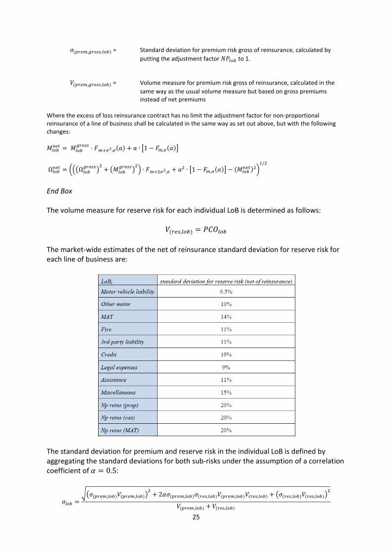
𝑉(𝑟𝑒𝑠,𝑙𝑜𝑏) = 𝑃𝐶𝑂𝑙𝑜𝑏 The market-wide estimates of the net of reinsurance standard deviation for reserve risk for each line of business are:

The standard deviation for premium and reserve risk in the individual LoB is defined by aggregating the standard deviations for both sub-risks under the assumption of a correlation coefficient of 𝛼 = 0.5:

𝜎𝑙𝑜𝑏 =��𝜎(𝑝𝑟𝑒𝑚,𝑙𝑜𝑏)𝑉(𝑝𝑟𝑒𝑚,𝑙𝑜𝑏)�

2 + 2𝛼𝜎(𝑝𝑟𝑒𝑚,𝑙𝑜𝑏)𝜎(𝑟𝑒𝑠,𝑙𝑜𝑏)𝑉(𝑝𝑟𝑒𝑚,𝑙𝑜𝑏)𝑉(𝑟𝑒𝑠,𝑙𝑜𝑏) + �𝜎(𝑟𝑒𝑠,𝑙𝑜𝑏)𝑉(𝑟𝑒𝑠,𝑙𝑜𝑏)�2

𝑉(𝑝𝑟𝑒𝑚,𝑙𝑜𝑏) + 𝑉(𝑟𝑒𝑠,𝑙𝑜𝑏)

26

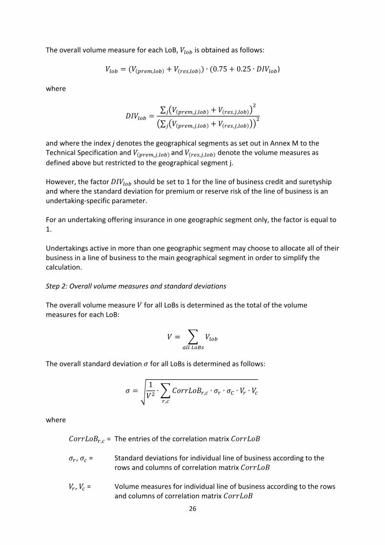
The overall volume measure for each LoB, 𝑉𝑙𝑜𝑏 is obtained as follows:

𝑉𝑙𝑜𝑏 = (𝑉(𝑝𝑟𝑒𝑚,𝑙𝑜𝑏) + 𝑉(𝑟𝑒𝑠,𝑙𝑜𝑏)) ∙ (0.75 + 0.25 ∙ 𝐷𝐼𝑉𝑙𝑜𝑏)

where

𝐷𝐼𝑉𝑙𝑜𝑏 =∑ �𝑉(𝑝𝑟𝑒𝑚,𝑗,𝑙𝑜𝑏) + 𝑉(𝑟𝑒𝑠,𝑗,𝑙𝑜𝑏)�

2𝑗

�∑ �𝑉(𝑝𝑟𝑒𝑚,𝑗,𝑙𝑜𝑏) + 𝑉(𝑟𝑒𝑠,𝑗,𝑙𝑜𝑏)�𝑗 �2

and where the index j denotes the geographical segments as set out in Annex M to the Technical Specification and 𝑉(𝑝𝑟𝑒𝑚,𝑗,𝑙𝑜𝑏) and 𝑉(𝑟𝑒𝑠,𝑗,𝑙𝑜𝑏) denote the volume measures as defined above but restricted to the geographical segment j. However, the factor 𝐷𝐼𝑉𝑙𝑜𝑏 should be set to 1 for the line of business credit and suretyship and where the standard deviation for premium or reserve risk of the line of business is an undertaking-specific parameter. For an undertaking offering insurance in one geographic segment only, the factor is equal to 1. Undertakings active in more than one geographic segment may choose to allocate all of their business in a line of business to the main geographical segment in order to simplify the calculation. Step 2: Overall volume measures and standard deviations The overall volume measure 𝑉 for all LoBs is determined as the total of the volume measures for each LoB:

𝑉 = � 𝑉𝑙𝑜𝑏𝑎𝑙𝑙 𝐿𝑜𝐵𝑠

The overall standard deviation 𝜎 for all LoBs is determined as follows:

𝜎 = �1𝑉2

∙�𝐶𝑜𝑟𝑟𝐿𝑜𝐵𝑟,𝑐 ∙ 𝜎𝑟 ∙ 𝜎𝐶 ∙ 𝑉𝑟 ∙ 𝑉𝑐𝑟,𝑐

where

𝐶𝑜𝑟𝑟𝐿𝑜𝐵𝑟,𝑐 = The entries of the correlation matrix 𝐶𝑜𝑟𝑟𝐿𝑜𝐵 𝜎𝑟, 𝜎𝑐 = Standard deviations for individual line of business according to the

rows and columns of correlation matrix 𝐶𝑜𝑟𝑟𝐿𝑜𝐵

𝑉𝑟, 𝑉𝑐 = Volume measures for individual line of business according to the rows and columns of correlation matrix 𝐶𝑜𝑟𝑟𝐿𝑜𝐵

27

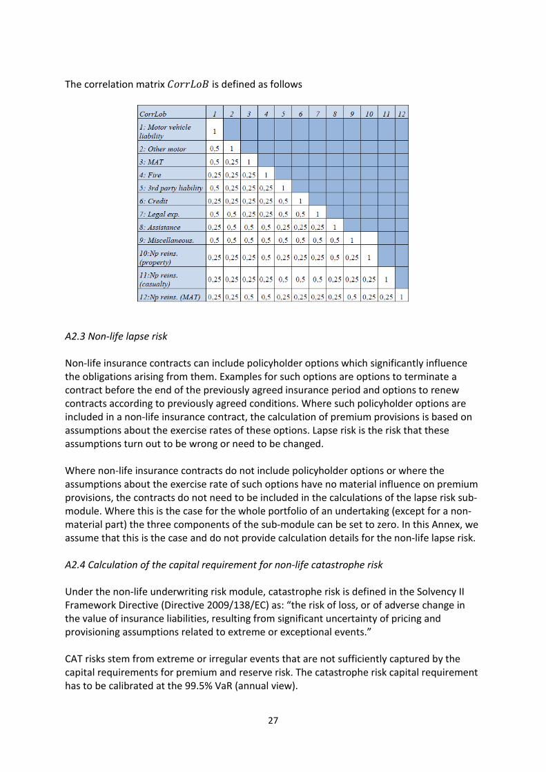
The correlation matrix 𝐶𝑜𝑟𝑟𝐿𝑜𝐵 is defined as follows

A2.3 Non-life lapse risk Non-life insurance contracts can include policyholder options which significantly influence the obligations arising from them. Examples for such options are options to terminate a contract before the end of the previously agreed insurance period and options to renew contracts according to previously agreed conditions. Where such policyholder options are included in a non-life insurance contract, the calculation of premium provisions is based on assumptions about the exercise rates of these options. Lapse risk is the risk that these assumptions turn out to be wrong or need to be changed. Where non-life insurance contracts do not include policyholder options or where the assumptions about the exercise rate of such options have no material influence on premium provisions, the contracts do not need to be included in the calculations of the lapse risk sub-module. Where this is the case for the whole portfolio of an undertaking (except for a non-material part) the three components of the sub-module can be set to zero. In this Annex, we assume that this is the case and do not provide calculation details for the non-life lapse risk. A2.4 Calculation of the capital requirement for non-life catastrophe risk Under the non-life underwriting risk module, catastrophe risk is defined in the Solvency II Framework Directive (Directive 2009/138/EC) as: “the risk of loss, or of adverse change in the value of insurance liabilities, resulting from significant uncertainty of pricing and provisioning assumptions related to extreme or exceptional events.” CAT risks stem from extreme or irregular events that are not sufficiently captured by the capital requirements for premium and reserve risk. The catastrophe risk capital requirement has to be calibrated at the 99.5% VaR (annual view).

28

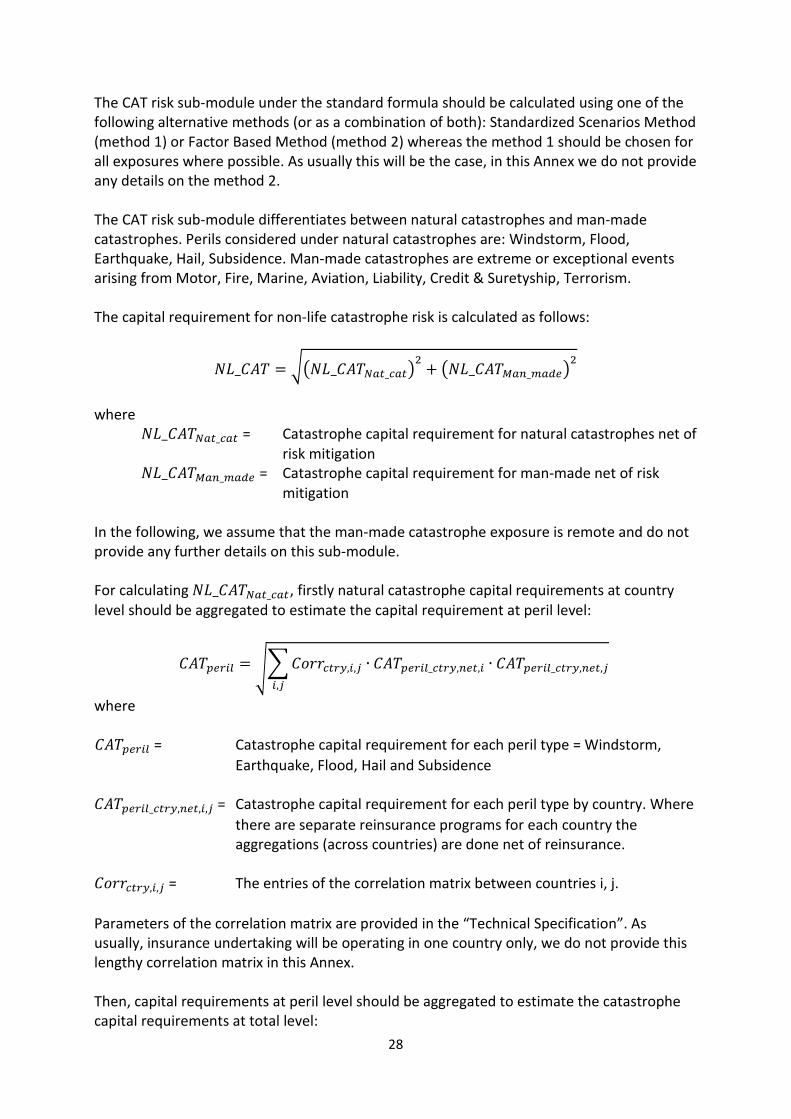
The CAT risk sub-module under the standard formula should be calculated using one of the following alternative methods (or as a combination of both): Standardized Scenarios Method (method 1) or Factor Based Method (method 2) whereas the method 1 should be chosen for all exposures where possible. As usually this will be the case, in this Annex we do not provide any details on the method 2. The CAT risk sub-module differentiates between natural catastrophes and man-made catastrophes. Perils considered under natural catastrophes are: Windstorm, Flood, Earthquake, Hail, Subsidence. Man-made catastrophes are extreme or exceptional events arising from Motor, Fire, Marine, Aviation, Liability, Credit & Suretyship, Terrorism. The capital requirement for non-life catastrophe risk is calculated as follows:

𝑁𝐿_𝐶𝐴𝑇 = ��𝑁𝐿_𝐶𝐴𝑇𝑁𝑎𝑡_𝑐𝑎𝑡�2

+ �𝑁𝐿_𝐶𝐴𝑇𝑀𝑎𝑛_𝑚𝑎𝑑𝑒�2

where

𝑁𝐿_𝐶𝐴𝑇𝑁𝑎𝑡_𝑐𝑎𝑡 = Catastrophe capital requirement for natural catastrophes net of risk mitigation

𝑁𝐿_𝐶𝐴𝑇𝑀𝑎𝑛_𝑚𝑎𝑑𝑒 = Catastrophe capital requirement for man-made net of risk mitigation

In the following, we assume that the man-made catastrophe exposure is remote and do not provide any further details on this sub-module. For calculating 𝑁𝐿_𝐶𝐴𝑇𝑁𝑎𝑡_𝑐𝑎𝑡, firstly natural catastrophe capital requirements at country level should be aggregated to estimate the capital requirement at peril level:

𝐶𝐴𝑇𝑝𝑒𝑟𝑖𝑙 = ��𝐶𝑜𝑟𝑟𝑐𝑡𝑟𝑦,𝑖,𝑗 ∙ 𝐶𝐴𝑇𝑝𝑒𝑟𝑖𝑙_𝑐𝑡𝑟𝑦,𝑛𝑒𝑡,𝑖 ∙ 𝐶𝐴𝑇𝑝𝑒𝑟𝑖𝑙_𝑐𝑡𝑟𝑦,𝑛𝑒𝑡,𝑗𝑖,𝑗

where 𝐶𝐴𝑇𝑝𝑒𝑟𝑖𝑙 = Catastrophe capital requirement for each peril type = Windstorm,

Earthquake, Flood, Hail and Subsidence 𝐶𝐴𝑇𝑝𝑒𝑟𝑖𝑙_𝑐𝑡𝑟𝑦,𝑛𝑒𝑡,𝑖,𝑗 = Catastrophe capital requirement for each peril type by country. Where

there are separate reinsurance programs for each country the aggregations (across countries) are done net of reinsurance.

𝐶𝑜𝑟𝑟𝑐𝑡𝑟𝑦,𝑖,𝑗 = The entries of the correlation matrix between countries i, j. Parameters of the correlation matrix are provided in the “Technical Specification”. As usually, insurance undertaking will be operating in one country only, we do not provide this lengthy correlation matrix in this Annex. Then, capital requirements at peril level should be aggregated to estimate the catastrophe capital requirements at total level:

29

𝑁𝐿_𝐶𝐴𝑇𝑁𝑎𝑡_𝑐𝑎𝑡 = ��𝐶𝑜𝑟𝑟𝑝𝑒𝑟𝑖𝑙,𝑖,𝑗 ∙ 𝐶𝐴𝑇𝑝𝑒𝑟𝑖𝑙,𝑛𝑒𝑡,𝑖 ∙ 𝐶𝐴𝑇𝑝𝑒𝑟𝑖𝑙,𝑛𝑒𝑡,𝑗𝑖,𝑗

where 𝑁𝐿_𝐶𝐴𝑇𝑁𝑎𝑡_𝑐𝑎𝑡 = Catastrophe capital requirement for non-life net of risk mitigation 𝐶𝐴𝑇𝑝𝑒𝑟𝑖𝑙,𝑛𝑒𝑡,𝑖,𝑗 = Catastrophe capital requirement for each peril. Where there are

separate reinsurance programs for each country the aggregations (across countries) are done net of reinsurance.

𝐶𝑜𝑟𝑟𝑝𝑒𝑟𝑖𝑙,𝑖,𝑗 = The entries of the correlation matrix between perils i, j. The peril correlation matrix 𝐶𝑜𝑟𝑟𝑝𝑒𝑟𝑖𝑙 is as follows

Notice that among all perils, some correlation is assumed for the pairs (windstorm; flood) and (windstorm; hail) only. The capital requirements per peril, country 𝐶𝐴𝑇𝑝𝑒𝑟𝑖𝑙_𝑐𝑡𝑟𝑦 gross of reinsurance are obtained from the sum insured aggregates per cresta zone, relativity factor for each zone and the zone aggregation matrix per country. Then the recoverables of reinsurance contract are taken into account. This provides the capital requirements per peril and country net of reinsurance 𝐶𝐴𝑇𝑝𝑒𝑟𝑖𝑙_𝑐𝑡𝑟𝑦,𝑛𝑒𝑡. For example, for earthquake, the calculation is as follows:

𝐶𝐴𝑇𝐸𝑄_𝑐𝑡𝑟𝑦 = 𝑄𝐶𝑇𝑅𝑌��𝐴𝐺𝐺𝑟.𝑐 ∙ 𝑊𝑇𝐼𝑉𝑍𝑂𝑁𝐸,𝑟 ∙ 𝑊𝑇𝐼𝑉𝑍𝑂𝑁𝐸,𝑐𝑟,𝑐

where 𝑊𝑇𝐼𝑉𝑍𝑂𝑁𝐸 = 𝐹𝑍𝑂𝑁𝐸 ∙ 𝑇𝐼𝑉𝑍𝑂𝑁𝐸 𝑇𝐼𝑉𝑍𝑂𝑁𝐸 = 𝑇𝐼𝑉𝑍𝑂𝑁𝐸_𝐹𝑖𝑟𝑒 + 𝑇𝐼𝑉𝑍𝑂𝑁𝐸_𝑀𝐴𝑇 𝑇𝐼𝑉𝑍𝑂𝑁𝐸_𝐹𝑖𝑟𝑒 = Total insured value for Fire and other damage by zone 𝑇𝐼𝑉𝑍𝑂𝑁𝐸_𝑀𝐴𝑇 = Total insured value for Marine by zone 𝑄𝐶𝑇𝑅𝑌 = 1 in 200 year factor for each country. These factors for different perils, countries are provided in Annex L5 to the “Technical Specification”

30

𝐴𝐺𝐺𝑟,𝑐 = Rows and columns of aggregation matrix by country. These values are

provided in the excel spreadsheet “parameters for non-life catastrophe” available from EIOPA website (European Insurance and Occupational Pensions Authority) under the QIS5 helper tabs

𝐹𝑍𝑂𝑁𝐸 = Relativity factors for each zone by country. These values are provided

in the excel spreadsheet “parameters for non-life catastrophe” available from EIOPA website (European Insurance and Occupational Pensions Authority) under the QIS5 helper tabs

𝑊𝑇𝐼𝑉𝑍𝑂𝑁𝐸 = Geographically weighted total insured value by zone Finally through taking into account risk mitigating effect of reinsurance, the capital requirement for earthquake net of reinsurance

𝐶𝐴𝑇𝐸𝑄_𝑐𝑡𝑟𝑦,𝑛𝑒𝑡 can be calculated. Capital requirements for other perils can be calculated analogously, for more details consult “Technical Specification”. Undertakings should note that netting down would not always be possible at a country level. For example you may have a European windstorm program in which case this would still be gross and not adjusted for risk mitigation until aggregating at country level. When netting down, undertakings should take care to adjust and interpret formulae accordingly. A2.5 Aggregation of capital requirements for non-life underwriting risk and default risk Aggregation of capital requirements for non-life underwriting risk and counterparty default risk takes into account some correlation assumptions. These assumptions are summarized by the following matrix (Technical Specification, SCR1.32)

The aggregation calculates with the following

𝑆𝐶𝑅𝑛𝑙+𝑑𝑒𝑓 = ��𝐶𝑜𝑟𝑟𝑖,𝑗 ∙ 𝑆𝐶𝑅𝑛𝑙 ∙ 𝑆𝐶𝑅𝑑𝑒𝑓𝑖,𝑗

31

Calculation of the capital requirement for the counterparty default 𝑆𝐶𝑅𝑑𝑒𝑓 risk is described in Annex A3.

32

Annex A3 Solvency capital requirements for reinsurance counterparty default risk under

Solvency II (QIS5) standard formula This specification follows “Technical Specification QIS5”, Section SCR.6 (SCR Counterparty risk module), pp. 193-203.

QIS5 differentiates between two kinds of counterparty risk exposure, denoted by type1 and type2 exposures. The class of type1 exposures covers the exposures which may not be diversified and where the counterparty is likely to be rated. Reinsurance arrangements belong to this type 1 class of exposures. The class of type2 exposures covers the exposures which are usually diversified and where the counterparty is likely to be unrated. Example of this class are receivables from intermediaries, policyholders debtors etc. Please refer to QIS5 Sections SCR6.2-6.4 for more details. We will consider only credit default risk exposure from reinsurance arrangements (type1) and assume there’s no exposure of type 2.

Solvency capital requirements for the type 1 of exposure can be calculated as (SCR6.6):

𝑆𝐶𝑅 = min (𝐿𝐺𝐷1 + 𝐿𝐺𝐷2 + ⋯+ 𝐿𝐺𝐷𝑁; 𝑞 ∙ √𝑉)

where

𝐿𝐺𝐷𝑖 = Loss-given-default for counterparty i

𝑞 = Quantile factor

𝑉 = Variance of the loss distribution for the credit risk exposure

According to SCR6.16, 𝐿𝐺𝐷𝑖 can be calculated as

𝐿𝐺𝐷𝑖 = max�(1 − 𝑅𝑅) ∙ (𝑅𝑒𝑐𝑜𝑣𝑒𝑟𝑎𝑏𝑙𝑒𝑠𝑖 + 𝑅𝑀𝑖 − 𝐶𝑜𝑙𝑙𝑎𝑡𝑒𝑟𝑎𝑙𝑖); 0�

where

𝑅𝑅 = Recovery rate for reinsurance arrangements. According to SCR6.52, for reinsurance arrangements, 𝑅𝑅 = 50% can be assumed.

𝑅𝑒𝑐𝑜𝑣𝑒𝑟𝑎𝑏𝑙𝑒𝑠𝑖 = Best estimate recoverables from the reinsurance contract i. We assume that 𝑅𝑒𝑐𝑜𝑣𝑒𝑟𝑎𝑏𝑙𝑒𝑠𝑖 = expected loss ceded to the reinsurance contract i plus reinsurance share on provisions for claims provisions.

𝐶𝑜𝑙𝑙𝑎𝑡𝑒𝑟𝑎𝑙𝑖 = Risk-adjusted value of collateral in relation to the reinsurance arrangement i. We assume 𝐶𝑜𝑙𝑙𝑎𝑡𝑒𝑟𝑎𝑙𝑖 = 0.

According to SCR6.17 and SCR6.32, Risk Mitigation 𝑅𝑀𝑖 can be calculated as

𝑅𝑀𝑖 = �𝑆𝐶𝑅𝑔𝑟𝑜𝑠𝑠 − 𝑆𝐶𝑅𝑛𝑒𝑡� ∙𝑅𝑒𝑐𝑜𝑣𝑒𝑟𝑎𝑏𝑙𝑒𝑠𝑖

𝑅𝑒𝑐𝑜𝑣𝑒𝑟𝑎𝑏𝑙𝑒𝑠𝑡𝑜𝑡𝑎𝑙

where

33

𝑆𝐶𝑅𝑔𝑟𝑜𝑠𝑠 = solvency capital requirements for underwriting risk calculated without reinsurance

𝑆𝐶𝑅𝑛𝑒𝑡 = solvency capital requirements for underwriting risk taking reinsurance into account

𝑅𝑒𝑐𝑜𝑣𝑒𝑟𝑎𝑏𝑙𝑒𝑠𝑖 = Best estimate recoverables from the reinsurance contract i.

𝑅𝑒𝑐𝑜𝑣𝑒𝑟𝑎𝑏𝑙𝑒𝑠𝑡𝑜𝑡𝑎𝑙 = Best estimate recoverables from all reinsurance contracts together.

According to SCR6.55, Quantile factor 𝑞 can be chosen as

𝑞 = �3 if √𝑉 ≤ 5% ⋅ (𝐿𝐺𝐷1 + 𝐿𝐺𝐷2 + ⋯+ 𝐿𝐺𝐷𝑁)5 else

Calculation of the variance 𝑉 is described in SCR6.7. We differentiate between counterparties belonging to different rating classes from AAA to CCC. We assume that in our case there are M rating classes for reinsurance counterparties. For each rating class j we first calculate 𝑦𝑗 and 𝑧𝑗 according to

𝑦𝑗 = 𝐿𝐺𝐷1 + 𝐿𝐺𝐷2 + ⋯+ 𝐿𝐺𝐷𝑁𝑗

𝑧𝑗 = 𝐿𝐺𝐷12 + 𝐿𝐺𝐷22 + ⋯+ 𝐿𝐺𝐷𝑁𝑗2

where the sums are over all counterparties in the rating class j and 𝑁𝑗 denotes the total number of counterparties in the rating class j.

Then, we calculate

𝑉 = (𝑢11 ∙ 𝑦1 ∙ 𝑦1 + 𝑢12 ∙ 𝑦1 ∙ 𝑦2 + ⋯+ 𝑢1𝑀 ∙ 𝑦1 ∙ 𝑦𝑀 + 𝑢21 ∙ 𝑦2 ∙ 𝑦1 + 𝑢22 ∙ 𝑦2 ∙ 𝑦2 + ⋯+ 𝑢2𝑀 ∙ 𝑦2 ∙ 𝑦𝑀 + ⋯+ 𝑢𝑀1 ∙ 𝑦𝑀 ∙ 𝑦1 + 𝑢𝑀2 ∙ 𝑦𝑀 ∙ 𝑦2 + ⋯+ 𝑢𝑀𝑀 ∙ 𝑦𝑀 ∙ 𝑦𝑀)+ (𝜈1 ∙ 𝑧1 + 𝜈2 ∙ 𝑧2 + ⋯+ 𝜈𝑀 ∙ 𝑧𝑀)

Finally, the coefficients 𝑢𝑖𝑗 and 𝜈𝑖 are calculated from the default probabilities valid for each different rating class

𝑢𝑖𝑗 =𝑝𝑖 ∙ (1 − 𝑝𝑖) ∙ 𝑝𝑗 ∙ (1 − 𝑝𝑗)

(1 + 𝛾) ⋅ �𝑝𝑖 + 𝑝𝑗� − 𝑝𝑖 ⋅ 𝑝𝑗

𝜈𝑖 =(1 + 2𝛾) ⋅ 𝑝𝑖 ⋅ (1 − 𝑝𝑖)

(2 + 2𝛾 − 𝑝𝑖)

where

𝛾 = 0.25

and probabilities 𝑝𝑖 are according to the following table

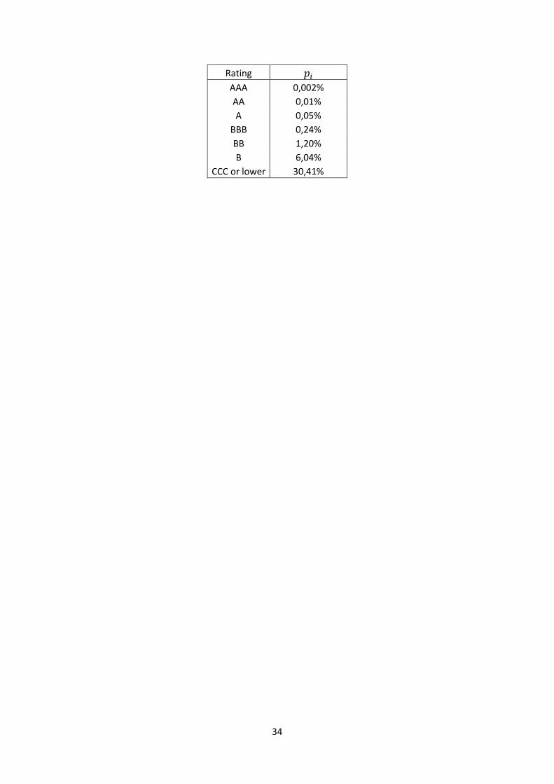
34

Rating 𝑝𝑖 AAA 0,002% AA 0,01% A 0,05%

BBB 0,24% BB 1,20% B 6,04%

CCC or lower 30,41%

35

Annex A4

Indicative pricing of non-proportional reinsurance for the sample portfolio

The indicative pricing of non-proportional reinsurance in this paper is based on the following formalism.

For an arbitrary non-proportional reinsurance layer, we first introduce the parameter called layer centroid which has the following property: Expected loss covered by a layer A xs B with the liability limit A and retention B is equal to the liability level of the layer multiplied by the expected number of losses higher than the centroid of this layer.

𝐸𝑥𝑝. 𝐿𝑜𝑠𝑠𝐴 𝑥𝑠 𝐵 = 𝐴 ∙ 𝐸𝑥𝑝.𝑁𝑙𝑜𝑠𝑠 > 𝐿𝐶 (A4.e1)

where 𝐸𝑥𝑝. 𝐿𝑜𝑠𝑠𝐴 𝑥𝑠 𝐵 denotes the expected loss covered by the layer A xs B and 𝐸𝑥𝑝.𝑁𝑙𝑜𝑠𝑠 > 𝐿𝐶 denotes the expected number of losses higher than the layer centroid.

From the above relation, we then derive for the net rate on line of the layer A xs B:

𝑁𝑒𝑡𝑅𝑜𝐿𝐴 𝑥𝑠 𝐵 ≜𝐸𝑥𝑝.𝐿𝑜𝑠𝑠𝐴 𝑥𝑠 𝐵

𝐴= 𝐸𝑥𝑝.𝑁𝑙𝑜𝑠𝑠 > 𝐿𝐶 (A4.e2)

Therefore, the layer price parameter NetRoL which is per definition equal to the expected loss covered by the layer divided by the layer liability limit can be calculated as the expected number of losses higher than the layer centroid.

For calculating 𝐸𝑥𝑝.𝑁𝑙𝑜𝑠𝑠 > 𝐿𝐶 we use the following relation

𝐸𝑥𝑝.𝑁𝑙𝑜𝑠𝑠 > 𝐿𝐶 = 𝐸𝑥𝑝.𝑁𝑙𝑜𝑠𝑠 > 𝐿𝐿𝐿 ⋅ 𝑃(𝑙𝑜𝑠𝑠 > 𝐿𝐶) (A4.e3)

= 𝐸𝑥𝑝.𝑁𝑙𝑜𝑠𝑠 > 𝐿𝐿𝐿 ⋅ �1 − 𝑃(𝑙𝑜𝑠𝑠 ≤ 𝐿𝐶)�

= 𝐸𝑥𝑝.𝑁𝑙𝑜𝑠𝑠 > 𝐿𝐿𝐿 ⋅ �1 − 𝐶𝐷𝐹(𝐿𝐶)�

where 𝐸𝑥𝑝.𝑁𝑙𝑜𝑠𝑠 > 𝐿𝐿𝐿 denotes the expected number of losses higher than lower loss limit (LLL) – the lower threshold of the loss severity distribution; 𝑃(𝑙𝑜𝑠𝑠 > 𝐿𝐶) denotes the probability that the loss severity is higher than layer centroid LC according to the chosen loss severity distribution and 𝐶𝐷𝐹(𝐿𝐶) denotes the cumulative distribution function of the chosen loss severity distribution. We further assume that 𝐿𝐶 > 𝐿𝐿𝐿 and that due to the fact that 𝐿𝐿𝐿 is the lower threshold of loss severity distribution 𝑃(𝑙𝑜𝑠𝑠 ≤ 𝐿𝐿𝐿) = 𝐶𝐷𝐹(𝐿𝐿𝐿) =0.

For calculating NetRoL according to (A4.e2) and (A4.e3), the value of the layer centroid is required. It can be shown that the following expression provides a good proxy:

Layer centroid of the layer A xs B ≅ �𝐵 ∙ (𝐴 + 𝐵) (A4.e4)

With the proxy (A4.e4), we can calculate NetRoL of an arbitrary layer A xs B which expresses the expected loss covered by the layer divided by the liability limit A. The market price of layer can be expressed with help of the parameter called GrossRoL which expresses the total of the expected loss covered by the layer and the costs allocated to the layer (costs of capital and management expenses) divided by the liability limit A.

36

𝐺𝑟𝑜𝑠𝑠𝑅𝑜𝐿𝐴 𝑥𝑠 𝐵 = 𝑁𝑒𝑡𝑅𝑜𝐿𝐴 𝑥𝑠 𝐵 + 𝐶𝑜𝑠𝑡𝑠

𝐴 (A4.e5)

Instead of estimating the costs in (A4.e5), we apply an approach as adopted by capital markets when pricing catastrophe bonds. It estimates the GrossRoL as a product of NetRoL and the factor called Multiple which expresses the relation of the gross layer price (which includes the expected loss and the allocated costs) to the pure expected loss.

𝐺𝑟𝑜𝑠𝑠𝑅𝑜𝐿𝐴 𝑥𝑠 𝐵 = 𝑀𝑢𝑙𝑡𝑖𝑝𝑙𝑒 ⋅ 𝑁𝑒𝑡𝑅𝑜𝐿𝐴 𝑥𝑠 𝐵 (A4.e6)

Expected loss covered by the layer A xs B and the reinsurance premium can be calculated from the net and gross rate on line according to the following:

𝐸𝑥𝑝. 𝐿𝑜𝑠𝑠𝐴 𝑥𝑠 𝐵 = 𝐴 ⋅ 𝑁𝑒𝑡𝑅𝑜𝐿𝐴 𝑥𝑠 𝐵 (A4.e7)

𝑅𝐼 𝑃𝑟𝑒𝑚𝑖𝑢𝑚𝐴 𝑥𝑠 𝐵 = 𝐴 ⋅ 𝐺𝑟𝑜𝑠𝑠𝑅𝑜𝐿𝐴 𝑥𝑠 𝐵 (A4.e8) Often, the expected loss and the price of an XL layer are expressed as rate on GNPI (gross net premium income) – premium retained under preceding proportional reinsurance (if any):

𝑁𝑒𝑡𝑅𝑎𝑡𝑒𝐴 𝑥𝑠 𝐵 = 𝐸𝑥𝑝. 𝐿𝑜𝑠𝑠𝐴 𝑥𝑠 𝐵 /𝐺𝑁𝑃𝐼 (A4.e9)

𝐺𝑟𝑜𝑠𝑠𝑅𝑎𝑡𝑒𝐴 𝑥𝑠 𝐵 = 𝑅𝐼 𝑃𝑟𝑒𝑚𝑖𝑢𝑚𝐴 𝑥𝑠 𝐵 /𝐺𝑁𝑃𝐼 (A4.e10) For the loss severity we chose censored Pareto distribution with the following cumulative distribution function

𝐶𝐷𝐹𝑃𝑎𝑟𝑒𝑡𝑜(𝑥) = 𝐿𝐿𝐿−𝛼−𝑥−𝛼

𝐿𝐿𝐿−𝛼−𝑈𝐿𝐿−𝛼 (A4.e11)

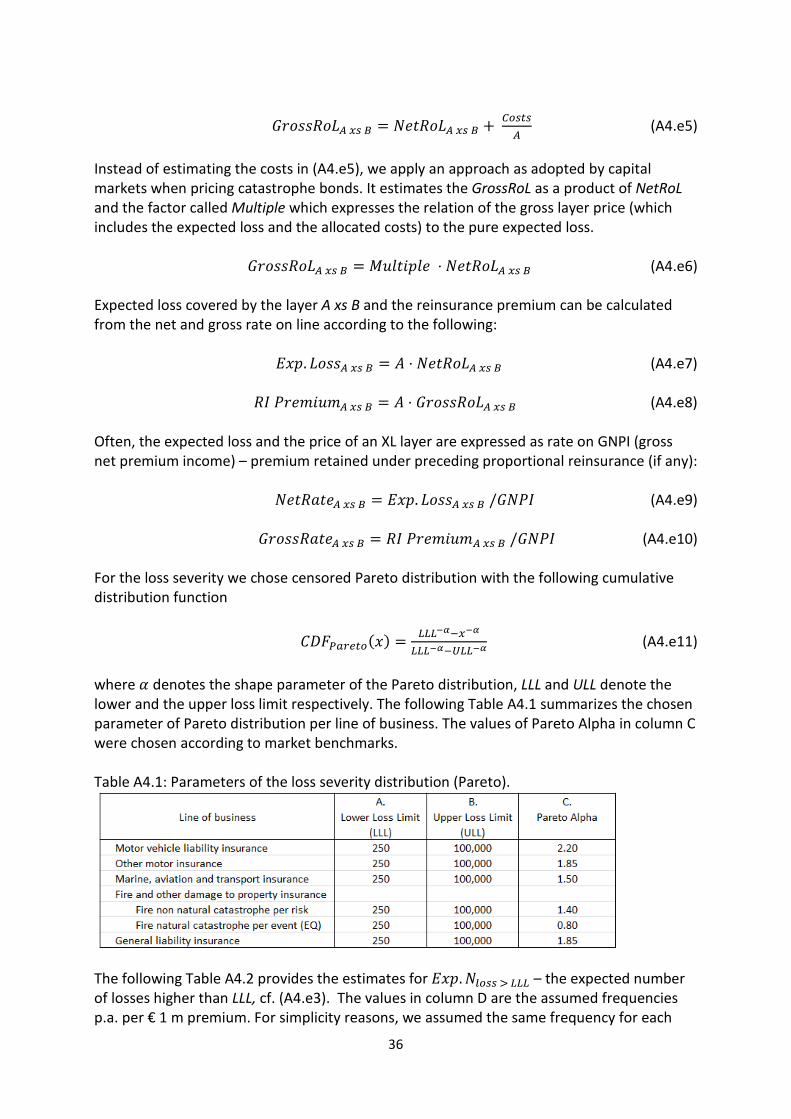
where 𝛼 denotes the shape parameter of the Pareto distribution, LLL and ULL denote the lower and the upper loss limit respectively. The following Table A4.1 summarizes the chosen parameter of Pareto distribution per line of business. The values of Pareto Alpha in column C were chosen according to market benchmarks. Table A4.1: Parameters of the loss severity distribution (Pareto).

The following Table A4.2 provides the estimates for 𝐸𝑥𝑝.𝑁𝑙𝑜𝑠𝑠 > 𝐿𝐿𝐿 – the expected number of losses higher than LLL, cf. (A4.e3). The values in column D are the assumed frequencies p.a. per € 1 m premium. For simplicity reasons, we assumed the same frequency for each

37

line of business, in-line with market benchmarks. The values in column F (except for fire earthquake) were obtained by multiplying the premiums in column E by the frequencies per € 1m premium (Table A4.1, column D). Obviously, the frequency of the earthquake loss does not depend on premium. It was estimated directly assuming the return period of 10 years for the loss higher than the lower loss threshold which translates into the frequency of 0.1. Table A4.2: Loss frequencies

Based on the formalism presented above (A4.e1 – A4.e11) and the parameters of loss severity and loss frequency distributions summarized in Tables A4.1 and A4.2, we estimated the prices of all XL layers throughout the paper. Below we provide calculation details for the layers of the original reinsurance structure, cf. Section 2.1. All other layers were priced analogously. Table A4.3 summarizes the parameters of the original reinsurance portfolio. Table A4.3: Parameters of the original reinsurance portfolio.

Based on the layer parameters provided in Table A4.3, columns I and J, we then calculated layer centroids and the expected number of losses higher than layer centroid, cf. Table A4.4.

38

Table A4.4: Layer centroids and expected number of losses higher than layer centroid

For calculating column M, we used (A4.e4) and for calculating column N (A4.e3) and (A4.e11). Please notice that in (A4.e11) the lower and upper loss limits from Table A4.4 columns K and L were used. These loss limits were obtained from the original loss limits (Table A4.1, columns A and B) through applying the retention ratio under the proportional reinsurance.

Table A4.5 provides the results for NetRoL and GrossRoL per line of business.

Table A4.5: Net and gross RoL

For calculating column O, we used (A4.e2). The Multiples in column P were assumed based on market benchmarks. For calculating column Q, we used (A4.e6).

Finally, Table A4.6 calculates the expected loss covered by the XL layers and the reinsurance premium as € figures as well as the net and gross rates on GNPI.

Table A4.6: Expected covered loss, reinsurance premium, net and gross rate on GNPI

For calculating column R, we used (A4.e7), for column S (A4.e7), for column T (A4.e9) and for column U (A4.e10). In the paper, these results were used in Tables 2.3.1 and 2.3.9, cf. Sections 2.3.1 and 2.3.4.