related securities and the cross-section of stock return ... · stock return momentum: evidence...
TRANSCRIPT
Related Securities and the Cross-section of
Stock Return Momentum: Evidence from
Credit Default Swaps (CDS)∗
Jongsub Lee†, Andy Naranjo‡, and Stace Sirmans§
Abstract
We document that related securities linked through firm fundamentals provide important cross-
market return performance information. During 2003-2015, we find significantly stronger stock
return momentum for entities whose past stock and CDS returns are in congruence versus
entities whose past stock and CDS returns disagree. A dynamic stock trading strategy based
on this cross-sectional performance differential earns an annualized alpha of nearly 18% with a
Sharpe ratio of 1.37, avoids crash risk, and is robust to out-of-sample tests using international
stocks. Relative pricing of credit across related securities explains, in part, the cross-section of
stock return momentum.
JEL Classification: G12, G14;Keywords: Related securities, CDS market, stock return momentum, CDS momentum, joint/disjointmomentum, momentum crashes, relative pricing of credit, capital structure arbitrage, marketsegmentation, stock market efficiency, international momentum
∗First draft: September 23, 2015; this version: November 15, 2016. We thank Sheridan Titman, MartiSubrahmanyam, Shrihari Santosh, Jacob Sagi, Menachem Brenner, Justin Birru, Jun Kyung Auh, as well asconference and seminar participants at the Ninth Annual Meeting of the Risk, Banking and Finance Society(Jerusalem, Israel), the 2016 Financial Econometrics and Empirical Asset Pricing Conference (SoFiE Co-sponsored, Lancaster, UK), the 2016 EFMA Annual Meeting (Basel, Switzerland), 2016 Northern FinanceAssociation Meeting (Mont Tremblant, Canada), the 2016 Chicago Quantitative Alliance (CQA) AnnualConference, Yonsei University, University of Arkansas, and SKKU for their helpful comments and suggestions.All remaining errors are our own.
†University of Florida, Assistant Professor, Tel: 352.273.4966, Email: [email protected]‡University of Florida, Emerson-Merrill Lynch Professor of Finance and Chairman of Finance Department,
Tel: 352.392.3781, Email: [email protected]§University of Arkansas, Assistant Professor, Tel: 850.459.2039, Email: [email protected]

Related Securities & Stock Return Momentum Page 1
1 Introduction
Firms often have related securities that trade concurrently in markets, which raises an im-
portant question on the extent to which related securities provide cross-market security
investment performance information. A long-standing empirical investments literature doc-
uments significant return momentum across a range of assets, including assets in both equity
and credit markets that are linked through common firm fundamentals.1 Given these re-
lated security fundamental linkages, do firms’ past equity and credit return signals agree or
disagree, and what do conflicting signals portend for return momentum? In this regard, the
literature documents momentum spillover effects from stocks to bonds (Gebhardt, Hvidk-
jaer, and Swaminathan, 2005) and from CDS to stocks (Lee, Naranjo, and Sirmans, 2014),
suggesting that while both the equity and credit exhibit momentum, individual securities
may be in different stages of underreaction or overreaction to fundamentals in their mo-
mentum cycles (Lee and Swaminathan, 2000). The degree of equity and credit momentum
cycle congruence may vary significantly in the cross-section with some high congruence firms
exhibiting a similar degree of underreaction or overreaction in the two markets and other low
congruence firms in strong discord, experiencing extreme overreaction in one market and se-
vere underreaction in the other market. Importantly, does heterogeneity in momentum cycle
congruence across firms impact future returns, trading behavior, and market efficiency?
In this paper, we examine the cross-section of stock return momentum with respect
to the performance of a related security, namely, credit default swaps (CDS). Both the
stock and CDS represent claims on the same underlying fundamentals of a firm, but their
market prices often evolve differentially, providing at times conflicting performance views.
We argue that jointly analyzing the performance of related securities provides clarity on the
stage of each individual security’s momentum cycle as well as insights into the strength of
the momentum effect. Strong stock performance coupled with weak CDS performance, for
example, may indicate that a stock is near the peak of an overreaction stage in its momentum
cycle and will soon reverse. If conflicting performance signals are associated with a greater
likelihood of reversal, a natural extension is to test whether hedging this disjoint group out of
1For details, see Jegadeesh and Titman (1993), Asness, Moskowitz, and Pedersen (2013), and manyothers for stock return momentum, Jostova, Nikolova, Philipov, and Stahel (2013) for corporate bond returnmomentum, and Lee, Naranjo, and Sirmans (2014) for CDS return momentum.

Related Securities & Stock Return Momentum Page 2
traditional momentum portfolios (Jegadeesh and Titman, 1993) helps avoid stock momentum
crashes (Daniel and Moskowitz, 2016). Existing studies on momentum crash risk (Daniel,
Jagannathan, and Kim, 2012; Grundy and Martin, 2001; Barroso and Santa-Clara, 2015;
Han, Zhou, and Zhu, 2016) have not examined the efficacy of a cross-sectional hedging
approach using multi-market momentum signals in lessening momentum tail risk. 2 Hence,
our study also provides novel economic insights that underlie well-known risk phenomena in
traditional single-signal momentum strategies.
Our arguments on multi-market momentum cycles and the resulting segmentation in
the cross-section of stock return momentum are motivated by recent segmentation theory.
Goldstein, Li, and Yang (2014) posit that stock markets are segmented by a diverse set
of investors with distinct trading opportunities and objectives. Simple investors trade as
speculators, participating only in a single stock market, while more sophisticated investors
also trade as hedgers, entering offsetting positions in both stock and CDS markets simul-
taneously. Market prices are therefore influenced not only by speculative trades reacting
to new stock market information but also to hedging trades reacting to the relative pricing
between the two markets. In practice, while retail and traditional institutional investors
primarily participate in stock markets, hedge funds that trade in both stock and CDS mar-
kets additionally have the opportunity to implement arbitrage trades when equity and credit
valuations become misaligned. Under this setup, at any point in time there is a portion of
the stock cross-section with diverging equity and credit prices that is more likely to attract
hedgers (i.e., contrarian traders) in proportion to speculators (i.e., momentum traders).
To further illustrate our point, consider two firms A and B in Figure 1 that both fall into
the proposed stock momentum winner portfolio at rebalancing date 0. Firm A is also a CDS
momentum winner (called a joint stock/CDS winner), but firm B is not a CDS momentum
winner (called a disjoint stock/CDS winner). Firm B’s stock price has become overvalued
relative to the level implied by its CDS counterpart and will therefore attract cross-market
convergence arbitrageurs intending to sell CDS protection while hedging the position by
selling stock (Yu, 2006; Duarte, Longstaff, and Yu, 2007; Kapadia and Pu, 2012). As a
2In an effort to further understand and hedge these costly momentum crashes, several studies haveinvestigated detecting the timing of the crash (Daniel, Jagannathan, and Kim, 2012), hedging out momentumportfolio time-varying market risks (Grundy and Martin, 2001), or statistically moderating the volatility ofthe strategy (Barroso and Santa-Clara, 2015; Han, Zhou, and Zhu, 2016).

Related Securities & Stock Return Momentum Page 3
result, firm B’s stock is more likely to experience a return reversal rather than momentum
in comparison to firm A’s stock. An interesting question is to what extent do contrarian
stock traders whose trades are motivated by cross-market price discrepancies relate to the
tendency of some stocks to exhibit reversal while others experience momentum?
To empirically investigate this idea, we decompose the traditional stock momentum strat-
egy (Jegadeesh and Titman (1993)) into two subgroups according to cross-sectional perfor-
mance ranking agreement between stock and CDS markets. We assign firms in the stock
momentum winner and loser portfolios as being either (1) joint entities whose past stock and
CDS performance signals are in agreement or (2) disjoint entities whose past stock returns
disagree with past CDS returns. Using a sample of 881 U.S. firms over the period 2003 to
2015, we find significant variation in the cross-section of stock momentum with respect to
related security performance. The performance of the joint component of stock momentum
exceeds that of the disjoint component by more than 20% per year (1.73% per month). In
other words, stocks are much more likely to exhibit a continuation of return momentum
when there is past performance agreement across related securities. In contrast, disjoint
entities, whose related security price paths are more likely to attract arbitrageurs, create a
drag on stock momentum performance and contribute proportionally more to momentum
crash risk (Daniel and Moskowitz (2016)). Upon revealing this segmentation structure in
the cross-section of stock momentum, we develop a set of novel momentum hedging strate-
gies that take advantage of the wide performance differential between the joint and disjoint
subgroups and produce risk-adjusted returns of up to 18% per year (1.47% per month). Put
together, our results suggest that related securities at times reduce stock price efficiency and
cause excess volatility due to induced market segmentation (Goldstein, Li, and Yang, 2014;
Boehmer, Chava, and Tookes, 2016).
We focus on a firm’s CDS as a related security to the firm’s stock for several reasons.
First, there is a clear structural link between stock and CDS prices through the firm’s capital
structure (Merton, 1974). Second, despite the theoretical link between the two markets,
they reveal information non-synchronously with different frequencies, speeds, and content
across entities and events (Acharya and Johnson, 2007; Ni and Pan, 2010; Qiu and Yu,
2012; Lee, Naranjo, and Sirmans, 2014).3 Third, CDS at-market spreads are consistent in
3Distinct information in the two markets could provide a more precise signal on firm prospects than a
Related Securities & Stock Return Momentum Page 4
their assessment of the underlying credit risk with stock prices without being confounded by
other liquidity-related factors (Friewald, Wagner, and Zechner, 2014).4 In sharp contrast,
studies that measure credit risk through corporate bond returns or credit ratings document
a “distress risk puzzle” in which expected stock returns are negatively related to credit
risk, which is hard to reconcile from a fundamentals perspective (Dichev, 1998; Campbell,
Hilscher, and Szilagyi, 2008; Avramov, Chordia, Jostova, and Philipov, 2009). Finally, as
Yu (2006) notes, instances of mispricing between stock and CDS markets offer attractive
opportunities for cross-market arbitraguers, suggesting that past CDS market performance
information may be useful in inferring future cross-market trading activity.
Using the Center for Research in Security Prices (CRSP) and Markit data, we identify
881 U.S. firms with actively trading stocks and five-year CDS contracts during 2003-2015.
To investigate the cross-section of stock momentum, we independently double-sort stocks
into five-by-five portfolios based on (1) the past 12-month stock return, skipping the most
recent month, and (2) the past CDS return over various horizons.5 We subgroup firms in the
stock momentum portfolios by labeling them as joint entities, entities that are both stock
winners (losers) and CDS winners (losers), or disjoint entities, entities that are stock winners
(losers) but not CDS winners (losers). We then implement the stock momentum strategy for
each of these two subgroups, creating joint stock/CDS momentum and disjoint stock/CDS
momentum strategies, and compare their performance.
We find that our joint stock/CDS momentum strategy significantly outperforms both
its counterpart disjoint stock/CDS momentum and the traditional single-signal stock mo-
mentum strategy (Jegadeesh and Titman, 1993) for all formation horizons of past CDS
returns, ranging from one to 12 months. The performance of joint stock/CDS momentum
peaks at the past four-month CDS performance signal, yielding 1.64% per month (1.45%
on a risk-adjusted basis) with an annualized Sharpe ratio of 0.81. The performance differ-
single market signal because related security prices often reveal signals that are relevant to their common firmfundamentals. For example, CDS at-market spreads are shown to predict upcoming credit rating changes(Hull, Predescu, and White, 2004; Flannery, Houston, and Partnoy, 2010; Chava, Ganduri, and Ornthanalai,2012; Lee, Naranjo, and Sirmans, 2014) and earnings surprises (Batta, Qiu, and Yu, 2016) in consistentdirections.
4Han, Subrahmanyam, and Zhou (2016) also find that the term structure of CDS spreads contains usefulinformation on future stock returns.
5The CDS holding period excess return (net of the risk-free rate) is defined as the profit and loss (P&L)of a CDS trading with a unit $1-notional using an International Swaps and Derivatives Association (ISDA)CDS standard pricing model.

Related Securities & Stock Return Momentum Page 5
ential between joint and disjoint stock/CDS momentum amounts to 1.73% per month with
a Sharpe ratio of 1.04. Our results are robust to risk adjustments, including exposure to
the market excess return, Fama and French (1993) size and value factors, Carhart (1997)
momentum factor, Pastor and Stambaugh (2003) traded liquidity factor, and Novy-Marx
(2015) earnings momentum factors (SUE and CAR3 ).6 We further show that, relative to
traditional stock-only signals, the two markets’ joint signals more precisely predict upcoming
corporate events in anticipated directions—joint winners (losers) are more likely to exhibit
faster (slower) growth in profits and more frequently undergo rating upgrades (downgrades).
This relative CDS market information advantage is particularly profound among distressed
entities as well as during high credit risk periods.
What explains the lackluster performance of momentum in disjoint entities? We offer a
relative pricing framework rationale and show that disjoint winner (loser) stocks substantially
underestimate (overestimate) firm credit risks relative to their levels implied by CDS prices.
To the extent that stock/CDS cross-market arbitrage is unlimited, any instances of credit risk
mispricing will be swiftly corrected by arbitrageurs whose trades cause the equity and credit
valuations to converge. This suggests that stocks that misprice the underlying credit risk
relative to the CDS may tend to display return reversal rather than momentum. Indeed,
we find that disjoint entities, during the four months leading up to momentum portfolio
formation, experience a nearly 30% widening in the discrepancy between their stock-implied
CDS spreads using the CreditGrades model and their observed at-market CDS spreads.
Then, post portfolio formation, the two spreads exhibit a tendency to converge. Importantly,
we do not find a similar pattern for joint entities. To show the relevance of cross-market
arbitrage to the reversing stock price pattern, we implement a capital structure arbitrage
trade for the most extreme disjoint entities (Yu, 2006; Duarte, Longstaff, and Yu, 2007;
Kapadia and Pu, 2012) and find significant profits of 1.28% per month.
Given the disparate performance between joint and disjoint stock/CDS momentum, we
examine how each contributes to the overall risk-return profile of the traditional stock mo-
mentum strategy. It is well-known that stock momentum exhibits an option-like payoff
structure with infrequent but severe crashes. In particular, Daniel and Moskowitz (2016)
6We also show that combining various horizons of past stock returns (Novy-Marx, 2012) does not yieldthe same performance enhancement over traditional momentum.

Related Securities & Stock Return Momentum Page 6
show that its time-varying beta exposure becomes strongly negative at the time a bear
market rebounds from its bottom, quickly eroding accumulated profits and leading to large
losses. Importantly, we find that only the disjoint momentum portfolio exhibits such behav-
ior in its time-varying beta exposure and sensitivity to bear market rebounds. We further
show that the joint-disjoint momentum performance differential is greatest during periods of
heightened volatility, precisely when momentum strategies produce less-than-stellar returns
(Daniel and Moskowitz (2016) and Barroso and Santa-Clara (2015)). These results suggest
that related security performance information could be useful in guarding against momen-
tum crash risk in part by providing timely updates on the strategy’s systematic market risk
exposure.
Building on our cross-section of stock return momentum intuition outlined above as well
as prior research on the time-varying risks of stock momentum, we introduce a set of powerful
hedging strategies that take advantage of the wide performance differential between the joint
and disjoint components of stock momentum. A static hedging strategy that invests 50% in
joint momentum and 50% in a disjoint contrarian strategy (purchasing disjoint losers and
selling short disjoint winners) avoids momentum crashes altogether and generates returns
of more than 10% per year (0.86% per month) with a Sharpe ratio of 1.04. Furthermore, a
dynamic hedging strategy that invests in joint momentum and hedges with a 50% disjoint
contrarian position only during periods of heightened volatility produces more than 19%
per year (1.59% per month) with a Sharpe ratio of 1.37. On a risk-adjusted basis, this
amounts to nearly 18% per year (1.47% per month). Our findings are complementary to
the momentum scaling approaches recently introduced by Daniel and Moskowitz (2016)
and Barroso and Santa-Clara (2015)—combining our cross-sectional approach with their
temporal scaling techniques leads to even higher Sharpe ratios of up to 1.61.
Lastly, we confirm our findings on related security performance and the cross-section
of stock momentum using a sample of 1,267 international firms headquartered outside of
the U.S. representing 49 countries. We find that our dynamic joint momentum hedging
strategy produces nearly 15% per year (1.21% per month) with a Sharpe ratio of 1.05.
Importantly, the joint and disjoint momentum segmentation structure is more pronounced
among more developed countries that generally face fewer impediments to arbitrage and
have investor capital that moves relatively quickly. Developed capital markets are also more
Related Securities & Stock Return Momentum Page 7
likely to exhibit cross-asset arbitrage capital flow, which our U.S. market results arguably
indicated as a potential cause of the segmented cross-section of stock return momentum.
Our international results are also consistent with the recent findings of Jacobs (2016) that
mispricing in stock markets appears to be as least as common in developed markets as it is
in developing and emerging markets.
Our contribution to the momentum literature is threefold. First, we show that related
security pricing information is important in identifying individual stock momentum cycles
(Lee and Swaminathan, 2000) through a relative pricing framework (Schaefer and Strebulaev,
2008; Friewald, Wagner, and Zechner, 2014; Bai and Wu, 2016; Yu, 2006; Duarte, Longstaff,
and Yu, 2007; Kapadia and Pu, 2012). Second, we provide a novel cross-sectional approach
to detect a group of stocks that are prone to reversal and are more sensitive to momentum
crash risk (Daniel and Moskowitz, 2016; Daniel, Jagannathan, and Kim, 2012; Grundy and
Martin, 2001; Barroso and Santa-Clara, 2015; Han, Zhou, and Zhu, 2016). Third, our new
and significantly profitable stock trading strategy that cross-sectionally combines momentum
and contrarian trades based on multi-market signals provides strong support for the recent
notion that related securities induce stock market segmentation, which, in turn, can reduce
stock price efficiency and cause excess volatility (Goldstein, Li, and Yang, 2014; Boehmer,
Chava, and Tookes, 2016).7
The remainder of this paper is organized as follows: Section 2 summarizes our data and
CDS return construction process. Section 3 presents our main results on related security
performance and the cross-section of stock return momentum. Section 4 introduces our new
momentum hedging strategies. Section 5 provides our international evidence. We conclude
in Section 6.
2 Data
Our U.S. data set consists of 881 firms from January 2003 to December 2015 for which there
is an actively traded stock and an active single-name CDS contract. Later in Section 5,
7 This interactive market (in)efficiency could also have implications for return momentum in other pairsof related securities (e.g., stocks and options, An, Ang, Bali, and Cakici, 2014).
Related Securities & Stock Return Momentum Page 8
we extend our U.S. data set to an international sample that includes 1,267 firms from 49
countries, and we provide corresponding details on our international sample construction
therein. For our U.S. firms, we obtain equity data from CRSP. We require the firm’s equity
to be ordinary common shares traded on the NYSE, AMEX or Nasdaq. We also require
each firm to have a market capitalization of at least $100 million and a price of at least $1
at the time of portfolio formation. CDS data are acquired from the Markit Group, a leading
financial information services company. All CDS contracts we consider are denominated
in U.S. dollars and have five-year maturities. We also impose a CDS activity filter at the
time of portfolio formation by eliminating contracts with a significant amount of missing
and stagnant observations. Specifically, we eliminate contracts that have missing spreads at
least 10% of days or stagnant spreads at least 90% of days over the prior six months. The
“Big Bang” protocol of April 2009 changed the standard for CDS contracts on a number
of dimensions, including a move from Modified Restructuring (MR) to No Restructuring
(XR) for North American corporate CDS contracts.8 As such, our database consists of
MR contracts prior to the “Big Bang” and XR contracts afterward. Markit constructs a
composite CDS spread using input from a variety of market makers and ensures each daily
observation passes a rigorous cleaning test to ensure accuracy and reliability.
Table 1 provides summary statistics and a correlation matrix of the variables used in
this study. The average firm in our sample has an equity market capitalization of $20.47
billion, a BBB S&P credit rating, and a CDS spread of 186 bps. Figure 2 shows the value-
weighted average corporate CDS spread over our sample period. As a measure of liquidity,
Markit reports on a daily basis each firm’s CDS market “depth,” or the number of distinct
contributors providing quotes used to construct the composite spread. Markit requires a
minimum of two contributors. The mean CDS depth of our sample is 6.77.
2.1 CDS Returns
To compute the CDS holding period (excess) return, we compute the profit or loss (P&L)
of a CDS over a given holding interval. We use an ISDA CDS standard pricing model to
compute the P&L. The P&L of a CDS trading with a unit $1-notional is what we term the
8For more details, visit www.markit.com/cds/announcements/resource/cds big bang.pdf.

Related Securities & Stock Return Momentum Page 9
CDS holding period excess return. This notion of CDS return is consistent with Berndt
and Obreja (2010), who view the protection seller’s position in a CDS as a long asset swap
position in the risky par-bonds issued by the same reference entity. Hence, the protection
seller’s position in a CDS could be viewed as a 100% levered risky par-bond position that
is financed at the risk-free rate, which serves as the basis for the notion of “excess” return.
We interchangeably use the terms – CDS holding period excess return, CDS holding period
return, and CDS return – throughout this manuscript. For more details regarding CDS
return computation, see Appendix C.
The summary statistics in Table 1 show that the mean (median) monthly CDS return
of our sample is 0.01% (0.01%) with a standard deviation of 2.57%. The simple correlation
between the stock return and CDS return is 0.037.
3 The Cross-Section of Stock Return Momentum
In this section, we uncover significant performance variation in the cross-section of the tra-
ditional Jegadeesh and Titman (1993) stock momentum strategy with respect to related
security performance. In particular, we show that considering the performance information
of both stock and CDS markets jointly sharpens signals on future firm fundamentals and
can be used to significantly improve the performance of stock momentum trading strategies.
Our primary empirical methodology is to decompose traditional stock momentum into
two parts based on firms’ cross-sectional performance ranking agreement between stock and
CDS markets. To do this, we conduct two independent sorts at the end of each month.
First, firms are sorted into five equally-sized portfolios based on their stock return over
the past 12 months, skipping the most recent month. Second, firms are sorted into five
equally-sized portfolios based on their CDS return over the past J months. The joint winner
portfolio, defined as JW ≡ WS ∩ WC , represents the overlap between the stock momentum
winner portfolio WS and the CDS momentum winner portfolio WC . Likewise, the joint loser
portfolio, defined as JL ≡ LS ∩ LC , represents the overlap between the stock momentum
loser portfolio LS and the CDS momentum loser portfolio LC . The disjoint winner (disjoint
loser) portfolio is the complement to the joint winner (joint loser) portfolio. That is, the
disjoint winner portfolio, defined as DW ≡ WS \ WC , includes all firms in the stock winner

Related Securities & Stock Return Momentum Page 10
portfolio that are not in the CDS winner portfolio. Similarly, the disjoint loser portfolio,
defined as DL ≡ LS \ LC , includes all firms in the stock loser portfolio that are not in the
CDS loser portfolio.
The joint stock/CDS momentum strategy (“joint momentum,” hereafter) purchases stocks
in the joint winner portfolio and sells short stocks in the joint loser portfolio. The disjoint
stock/CDS momentum strategy (“disjoint momentum,” hereafter) purchases stocks in the
disjoint winner portfolio and sells short stocks in the disjoint loser portfolio. Positions are
held and rebalanced after K months. We focus on the baseline case K = 1m in this paper.
Ultimately, our stock momentum decomposition procedure can be summarized as:
Stock Momentum ≡ (WS−LS)
⎧⎪⎪⎨
⎪⎪⎩
Joint Stock/CDS Momentum ≡ (WS ∩ WC) − (LS ∩ LC)
Disjoint Stock/CDS Momentum ≡ (WS \ WC) − (LS \ LC).
Table 2 reports the performance of our joint momentum strategy over the period January
2003 to December 2015 using CDS formation horizons ranging from one month (J = 1m) to
twelve months (J = 12m).9 We find that CDS formation periods of J = 3m through J = 5m
show positive returns for the joint momentum strategy at the 1% to 5% statistical significance
level (see column 3). All CDS formation periods from J = 1m to J = 12m produce positive
alpha coefficients (see column 4) using a four-factor model that includes the Fama-French
market, size, and value factors as well as an in-sample stock momentum factor (denoted as
UMDS hereafter).10 The four-month formation period (J = 4m) maximizes the strategy’s
performance, producing a return of 1.64% per month (t-statistic of 2.83), an annualized
Sharpe ratio of 0.81, and an alpha of 1.45% per month (t-statistic of 4.24). 11 The joint
winner portfolio generates a return of 1.49% per month (t-statistic of 2.69), while the joint
loser portfolio produces a return of -0.15% per month (t-statistic of -0.16). Figure 3 plots
the cumulative profits of our in-sample stock momentum strategy (in black) as well as each
of the joint (in blue) and disjoint (in red) components of stock momentum using a CDS
9CDS momentum portfolios are constructed without a one-month gap between the formation and holdingperiods.
10The UMDS factor is constructed in-sample using quintiles of firms’ past 12-month stock return (J =12m), skipping the most recent month, and a holding period of one month (K = 1m).
11Our Internet Appendix shows that average monthly risk-adjusted returns are positive and statisticallysignificant at the 1% level at least up to a six-month holding period (K = 6m).

Related Securities & Stock Return Momentum Page 11
formation horizon of J = 4m.
The last three columns of Table 2 report the monthly return differentials between joint
momentum, disjoint momentum, and traditional stock momentum. The performance ad-
vantage of joint momentum over both traditional stock momentum and disjoint momentum
is positive and statistically significant at the 1% to 5% level for all CDS formation periods.
The performance advantage of joint momentum is greatest at the four-month CDS return
horizon, outpacing traditional stock momentum by 1.34% per month (t-statistic of 4.08 and
Sharpe ratio of 1.05) and exceeding disjoint momentum by 1.73% per month (t-statistic of
3.94 and Sharpe ratio of 1.04).
3.1 Risk-adjusted Performance
Next, we test whether our joint stock/CDS momentum profits are explained by exposures to
commonly-used asset pricing factors. We consider the market excess return factor (MKT ),
Fama and French (1993) size and value factors (SMB and HML, respectively), a “localized”
stock momentum factor using firms in our sample (UMDS), the Pastor and Stambaugh
(2003) traded liquidity factor (LIQ), and Novy-Marx (2015) earnings momentum factors
(SUE and CAR3 ). The factors MKT, SMB, and HML are from Ken French’s website.12 SUE
and CAR3 are broad stock market factors constructed using the standardized unexpected
earnings and the three-day cumulative abnormal return around the most recent earnings
announcement, respectively.13 Using OLS with Newey-West standard errors and a lag length
of 12 months, we estimate:
rPt = αP + β′PFt + ePt, (1)
where rPt is the long-short momentum portfolio returns, αP is the portfolio’s alpha, and Ft
is a vector of stock market risk factors.
Table 3 presents alpha coefficients from the time-series regressions. Columns 1 and 2
show that the average risk-adjusted monthly return of our in-sample stock momentum is not
statistically different from zero over the period 2003 to 2015. However, segmenting stock
momentum into its joint and disjoint components reveals sharp contrasting performance.
12See http://mba.tuck.dartmouth.edu/pages/faculty/ken.french/data library.html.13 We follow similar construction procedures to Novy-Marx (2015). Appendix B provides a more detailed
definition of our two earnings-based factors.
Related Securities & Stock Return Momentum Page 12
Columns 3 to 5 show that the alpha coefficients of joint momentum are all positive and
statistically significant at the 1% to 5% level across all three models, ranging from 1.21% per
month (column 5) to 1.56% per month (column 4). In contrast, all three models explaining
disjoint momentum show alpha coefficients that are economically and statistically negative,
ranging from -0.45% (column 6) to -0.49% (column 8). These results confirm our segmenta-
tion structure of stock return momentum and further reveal that it is not explained by size,
value, liquidity, or earnings-based factors.14
3.2 Future Firm Fundamentals
Our a priori expectation is that past stock and CDS performance signals, if optimally com-
bined, could more sharply identify price underreactions to firm fundamentals. 15 The joint
signals could capture price underreactions to earnings announcements, but they are not lim-
ited to capturing only earnings-related information. The significant joint momentum alpha of
1.21% per month in column 5 of Table 3 suggests that the joint-market signals capture other
upcoming corporate events that also materially affect common firm fundamentals through a
channel other than earnings surprises.16 An upcoming change in credit rating, for example,
is such an event (Kisgen, 2006, 2007).
To directly test whether joint stock/CDS signals more precisely capture future firm funda-
mentals in correctly anticipated directions, Table 4 presents results on whether joint winners
(losers) exhibit faster (slower) growth in gross profits and more frequent credit rating en-
hancements (deteriorations) in the 18 months following the portfolio formation date. For
comparison, we also show these developments for the disjoint winner and loser portfolios
and report differences with respect to traditional stock momentum. Our purpose here is to
identify the marginal value of past CDS performance signals in more accurately anticipating
the state of future firm fundamentals. When generating the cumulative six to 18-month
14Our Internet Appendix further shows the robustness of our joint momentum strategy to a larger setof factors, including a Fama-French five-factor model with operating profitability (RMW ) and investment(CMA) factors, Novy-Marx (2013) gross profitability factor (GPROF ), Asness, Frazzini, and Pedersen (2014)quality-minus-junk factor (QMJ ), the Stambaugh and Yuan (2016) mispricing factors (MGMT and PERF ),short-term reversal factor (STREV ), and long-term reversal factor (LTREV ).
15In Table 3, two of the most significant factor loadings for the joint momentum strategy are on thefundamental earnings momentum factors (1.77 for βSUE and 1.17 for βCAR3).
16As evidence of this, Internet Appendix shows that our CDS-based joint momentum strategy explainsvarious SUE-based strategies but not vice-versa.
Related Securities & Stock Return Momentum Page 13
percentage growth in gross profits and S&P rating changes, we avoid an overlapping obser-
vations problem by compiling one-month statistics over relevant time intervals (Jegadeesh
and Titman, 1993).17
Table 4 shows that firm profits grow much faster in the joint momentum portfolio than
both the traditional momentum and disjoint momentum portfolios. For example, after six
months following the portfolio formation date, the wedge in gross profits growth between the
joint winner and joint loser portfolios amounts to 13.64%, which is 4.01% higher than that
of traditional stock winner and loser portfolios and 5.72% (= 13 .64% − 7.92%) higher than
that of disjoint winner and loser portfolios. We further find that net credit enhancement
between the joint winner and loser portfolios (-0.52) is more than twice as likely as in
traditional stock momentum portfolios and more than three times as likely as in the disjoint
momentum portfolios. Our results in Table 4 indicate a potential information advantage for
joint momentum signals in predicting future firm prospects.
3.3 Marginal Information in the Past CDS Performance over Past
Stock Performance
One could argue that past CDS returns have no marginal information over past stock returns,
and therefore our joint stock/CDS momentum strategy is merely a finer sorting strategy
using multi-horizon stock return signals.18 To directly address these potential concerns, we
perform several exercises to showcase the marginal value of past CDS performance signals
for future stock returns.
Panel A of Table 5 presents alpha coefficients of various long-short momentum strategies
using a formation period of four months (J = 4m). The alpha coefficient is based on a model
that includes MKT, SMB, HML, and UMDS factors. Each strategy purchases stocks in the
highest quintile while selling short stocks in the lowest quintile. In the first two columns
labeled “Raw Signal,” we contrast the value of the past CDS performance signal relative
to the past stock performance signal for future stock momentum profits. A long/short
17For instance, the six-month period cumulative gross profits growth (%) is computed by summing theone-month profits growth (%) of six momentum portfolios formed in the current month, one month prior,two months prior, three months prior, four months prior, and five months prior.
18Novy-Marx (2015) shows that various horizon past stock returns have different signals about continuingprice momentum or reversal.
Related Securities & Stock Return Momentum Page 14
momentum strategy that simply purchases (sells short) the stock of firms with good (bad)
past four-month CDS performance produces a statistically significant alpha of 0.88% per
month (column 2). In fact, this stock momentum strategy using only past CDS performance
outperforms a similarly-constructed strategy based on the past four-month stock performance
by 0.90% per month [= 0.88% − (−0.02%), see column 1].
Positive correlation in stock and CDS performance implies that past CDS winners tend
to have better historical stock performance than past CDS losers. To adjust for this potential
bias in our first two column results, we perform a conditional sort similar to that of Novy-
Marx (2015) by first creating quintiles of the past four-month stock return and then creating
conditional quintiles of the four-month CDS return that draws equally from the stock return
quintiles. This procedure ensures a minimal past stock performance differential between
CDS winners and CDS losers. In columns 3 and 4, labeled “Conditional Signal,” we show
the results of two conditional sorts, rS,4 | rC,4 and rC,4 | rS,4, respectively. In column 4
we find that even after conditioning on past stock performance, the CDS-based strategy
generates a positive alpha of 0.74% that is statistically significant at the 1% level and has
a Sharpe ratio of 0.75, providing further evidence that the historical CDS performance
signal itself does, in fact, have value for future stock returns. In contrast, conditioning
the stock-based strategy on past CDS performance worsens its risk-adjusted performance
to a statistically insignificant -0.27% per month. The strategy based on the conditional
stock signal underperforms a similar strategy based on the conditional CDS signal strategy
by 1.01% per month (= 0.74% − −0.27%). This sharply identifies the marginal predictive
power that the past CDS performance signal has on future stock returns.19
3.3.1 Marginal Information in CDS Performance Signals: The Role of CDS
Market Depth and Distress Risk
When is the CDS market information most useful in enhancing traditional stock momen-
tum profits? Credit risk often becomes a greater concern to equity investors in distressed
markets, so we might expect CDS performance signals to be more relevant among low-grade
firms or during periods of high uncertainty and widening credit spreads. Furthermore, more
19Our Internet Appendix further confirms the marginal value in the past CDS return using various forma-tion horizons from one to 12 months and also shows that a multi-term stock momentum strategy does notproduce statistically significant positive alpha.
Related Securities & Stock Return Momentum Page 15
participation in a firm’s CDS market may correspond to more informed spreads, particularly
if CDS trading is motivated by endogenous credit risk hedging demands as explored by Qiu
and Yu (2012). To investigate these possibilities, we consider both cross-sectional and time
series effects by decomposing our sample firms and sample period into subgroups based on
CDS market depth and levels of distress risk. We use Markit’s reported CDS contract depth
as a measure of CDS market participation and S&P credit ratings or five-year CDS spread
levels as a proxy for corporate credit risk.
Panel A of Table 5 shows that higher depth CDS contracts are relatively more informative
about future stock returns. The conditional CDS-based strategy in column 4 generates
a statistically insignificant alpha of -0.03% per month among low CDS depth firms and
a statistically significant 0.94% per month (t-statistic of 3.88) among high depth firms.
Next, dividing the sample of firms based on S&P credit rating shows that CDS performance
signals are informative for both investment grade and junk grade firms with slightly greater
predictability among junk grade firms. The conditional CDS-based strategy generates an
alpha of 1.28% per month (t-statistic of 3.61) among junk grade firms and 0.52% (t-statistic
of 2.46) among investment grade firms. Similarly, dividing the sample into periods when
the value-weighted average corporate CDS spread is above and below its sample period
median (0.73%) shows that the CDS signal has important information for future stock returns
during both periods, with slightly stronger results during high risk states. The Joint-Disjoint
performance differential shows alpha coefficients of 1.60% (t-statistic of 2.80) during the low
risk period and 2.59% (t-statistic of 5.39) during the high risk period.
Altogether, our results in Table 5 highlight the increased relative information benefits of
the CDS performance signal when the CDS market is active and the level of distress risk is
high. As the region of equity payoffs approaches the firm’s default boundary, any underre-
action signals on future firm fundamentals could be sharpened out by jointly examining the
past performance of both equity securities and CDS contracts.
Related Securities & Stock Return Momentum Page 16
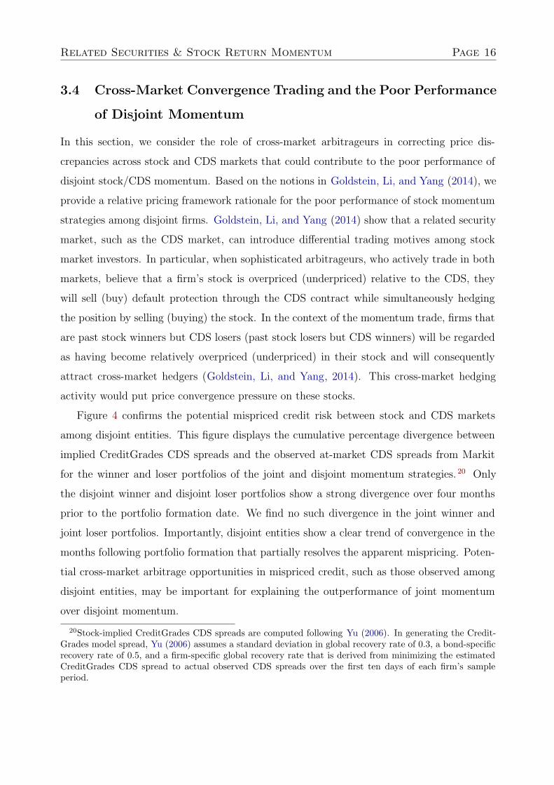
3.4 Cross-Market Convergence Trading and the Poor Performance
of Disjoint Momentum
In this section, we consider the role of cross-market arbitrageurs in correcting price dis-
crepancies across stock and CDS markets that could contribute to the poor performance of
disjoint stock/CDS momentum. Based on the notions in Goldstein, Li, and Yang (2014), we
provide a relative pricing framework rationale for the poor performance of stock momentum
strategies among disjoint firms. Goldstein, Li, and Yang (2014) show that a related security
market, such as the CDS market, can introduce differential trading motives among stock
market investors. In particular, when sophisticated arbitrageurs, who actively trade in both
markets, believe that a firm’s stock is overpriced (underpriced) relative to the CDS, they
will sell (buy) default protection through the CDS contract while simultaneously hedging
the position by selling (buying) the stock. In the context of the momentum trade, firms that
are past stock winners but CDS losers (past stock losers but CDS winners) will be regarded
as having become relatively overpriced (underpriced) in their stock and will consequently
attract cross-market hedgers (Goldstein, Li, and Yang, 2014). This cross-market hedging
activity would put price convergence pressure on these stocks.
Figure 4 confirms the potential mispriced credit risk between stock and CDS markets
among disjoint entities. This figure displays the cumulative percentage divergence between
implied CreditGrades CDS spreads and the observed at-market CDS spreads from Markit
for the winner and loser portfolios of the joint and disjoint momentum strategies. 20 Only
the disjoint winner and disjoint loser portfolios show a strong divergence over four months
prior to the portfolio formation date. We find no such divergence in the joint winner and
joint loser portfolios. Importantly, disjoint entities show a clear trend of convergence in the
months following portfolio formation that partially resolves the apparent mispricing. Poten-
tial cross-market arbitrage opportunities in mispriced credit, such as those observed among
disjoint entities, may be important for explaining the outperformance of joint momentum
over disjoint momentum.
20Stock-implied CreditGrades CDS spreads are computed following Yu (2006). In generating the Credit-Grades model spread, Yu (2006) assumes a standard deviation in global recovery rate of 0.3, a bond-specificrecovery rate of 0.5, and a firm-specific global recovery rate that is derived from minimizing the estimatedCreditGrades CDS spread to actual observed CDS spreads over the first ten days of each firm’s sampleperiod.
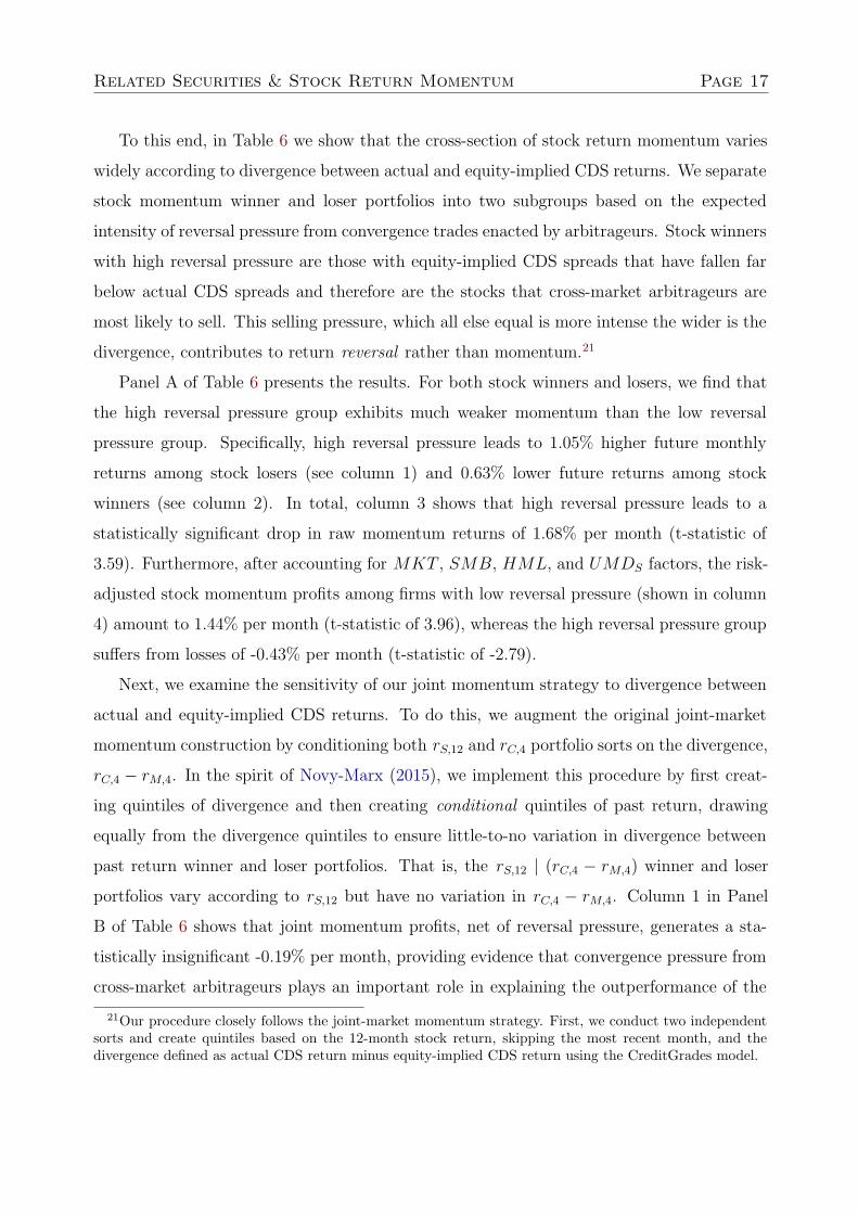
Related Securities & Stock Return Momentum Page 17
To this end, in Table 6 we show that the cross-section of stock return momentum varies
widely according to divergence between actual and equity-implied CDS returns. We separate
stock momentum winner and loser portfolios into two subgroups based on the expected
intensity of reversal pressure from convergence trades enacted by arbitrageurs. Stock winners
with high reversal pressure are those with equity-implied CDS spreads that have fallen far
below actual CDS spreads and therefore are the stocks that cross-market arbitrageurs are
most likely to sell. This selling pressure, which all else equal is more intense the wider is the
divergence, contributes to return reversal rather than momentum.21
Panel A of Table 6 presents the results. For both stock winners and losers, we find that
the high reversal pressure group exhibits much weaker momentum than the low reversal
pressure group. Specifically, high reversal pressure leads to 1.05% higher future monthly
returns among stock losers (see column 1) and 0.63% lower future returns among stock
winners (see column 2). In total, column 3 shows that high reversal pressure leads to a
statistically significant drop in raw momentum returns of 1.68% per month (t-statistic of
3.59). Furthermore, after accounting for MKT , SMB, HML, and UMDS factors, the risk-
adjusted stock momentum profits among firms with low reversal pressure (shown in column
4) amount to 1.44% per month (t-statistic of 3.96), whereas the high reversal pressure group
suffers from losses of -0.43% per month (t-statistic of -2.79).
Next, we examine the sensitivity of our joint momentum strategy to divergence between
actual and equity-implied CDS returns. To do this, we augment the original joint-market
momentum construction by conditioning both rS,12 and rC,4 portfolio sorts on the divergence,
rC,4 − rM,4. In the spirit of Novy-Marx (2015), we implement this procedure by first creat-
ing quintiles of divergence and then creating conditional quintiles of past return, drawing
equally from the divergence quintiles to ensure little-to-no variation in divergence between
past return winner and loser portfolios. That is, the rS,12 | (rC,4 − rM,4) winner and loser
portfolios vary according to rS,12 but have no variation in rC,4 − rM,4. Column 1 in Panel
B of Table 6 shows that joint momentum profits, net of reversal pressure, generates a sta-
tistically insignificant -0.19% per month, providing evidence that convergence pressure from
cross-market arbitrageurs plays an important role in explaining the outperformance of the
21Our procedure closely follows the joint-market momentum strategy. First, we conduct two independentsorts and create quintiles based on the 12-month stock return, skipping the most recent month, and thedivergence defined as actual CDS return minus equity-implied CDS return using the CreditGrades model.
Related Securities & Stock Return Momentum Page 18
joint stock/CDS momentum strategy.
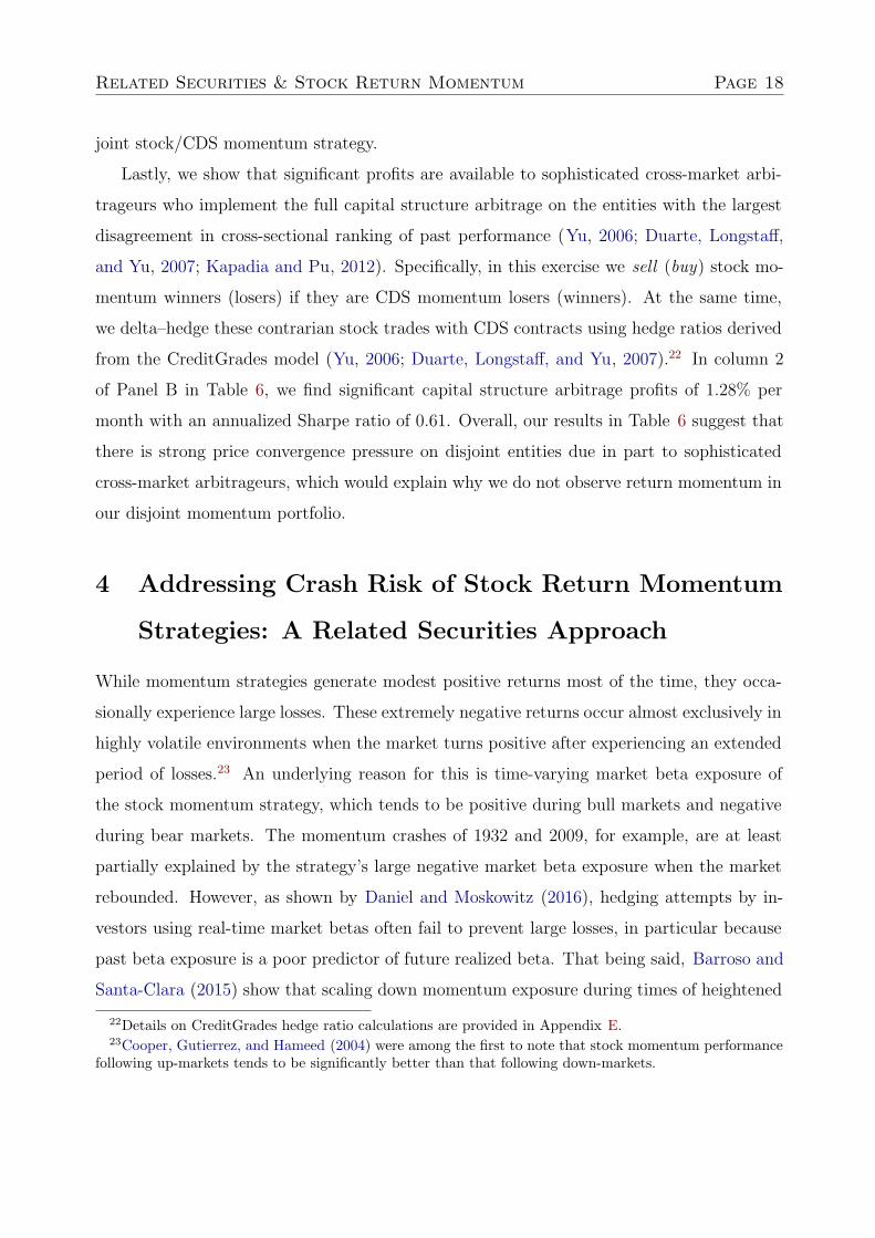
Lastly, we show that significant profits are available to sophisticated cross-market arbi-
trageurs who implement the full capital structure arbitrage on the entities with the largest
disagreement in cross-sectional ranking of past performance (Yu, 2006; Duarte, Longstaff,
and Yu, 2007; Kapadia and Pu, 2012). Specifically, in this exercise we sell (buy) stock mo-
mentum winners (losers) if they are CDS momentum losers (winners). At the same time,
we delta–hedge these contrarian stock trades with CDS contracts using hedge ratios derived
from the CreditGrades model (Yu, 2006; Duarte, Longstaff, and Yu, 2007).22 In column 2
of Panel B in Table 6, we find significant capital structure arbitrage profits of 1.28% per
month with an annualized Sharpe ratio of 0.61. Overall, our results in Table 6 suggest that
there is strong price convergence pressure on disjoint entities due in part to sophisticated
cross-market arbitrageurs, which would explain why we do not observe return momentum in
our disjoint momentum portfolio.
4 Addressing Crash Risk of Stock Return Momentum
Strategies: A Related Securities Approach
While momentum strategies generate modest positive returns most of the time, they occa-
sionally experience large losses. These extremely negative returns occur almost exclusively in
highly volatile environments when the market turns positive after experiencing an extended
period of losses.23 An underlying reason for this is time-varying market beta exposure of
the stock momentum strategy, which tends to be positive during bull markets and negative
during bear markets. The momentum crashes of 1932 and 2009, for example, are at least
partially explained by the strategy’s large negative market beta exposure when the market
rebounded. However, as shown by Daniel and Moskowitz (2016), hedging attempts by in-
vestors using real-time market betas often fail to prevent large losses, in particular because
past beta exposure is a poor predictor of future realized beta. That being said, Barroso and
Santa-Clara (2015) show that scaling down momentum exposure during times of heightened
22Details on CreditGrades hedge ratio calculations are provided in Appendix E.23Cooper, Gutierrez, and Hameed (2004) were among the first to note that stock momentum performance
following up-markets tends to be significantly better than that following down-markets.

Related Securities & Stock Return Momentum Page 19
total volatility of the momentum strategy itself is effective in reducing crash risk mostly be-
cause the strategy-specific component of momentum risk is highly autocorrelated. Likewise,
forecasting momentum returns using their historic relation to market volatility levels is also
useful in developing dynamic momentum strategies with smoother performance (Daniel and
Moskowitz (2016)). A common theme in the literature is that performance can be signifi-
cantly improved by scaling back exposure to the momentum strategy when volatility levels
become elevated.
Building on our insights from Section 3 as well as prior research on the time-varying risks
of stock momentum, we develop a set of implementable momentum hedging strategies that
utilize “cross-sectional” related security performance information to enhance the risk-return
profile of traditional stock momentum. These novel strategies are rooted in the robust per-
formance differential between the joint and disjoint segments of stock momentum, which we
have shown to be statistically positive for all formation horizons of CDS return and unex-
plained by common risk factors. In this section, we start by showing significant asymmetry
in option-like payoff risk between our joint and disjoint momentum strategies when a bear
market rebounds from its bottom. We further show that the joint-disjoint performance dif-
ferential is greatest during periods of heightened volatility, precisely when expected stock
momentum returns and Sharpe ratios are low, making it a particularly useful risk man-
agement tool to improve the risk-return profile of traditional stock momentum strategies.
Lastly, we present our momentum hedging strategies that provide superior performance to
the traditional stock momentum strategy.
To test whether our joint and disjoint momentum portfolios show severe option-like payoff
risk when a bear market rebounds from its bottom, we use the following test specification
in Daniel and Moskowitz (2016):
rMOMt = (α0 + αIBIB) + [βMKT + IB(βMKT×IB + IUβMKT×IB×IU )]rMKTt + eMOMt, (2)
where rMOMt is the momentum portfolio return, IB is an ex ante bear market indicator that
takes the value of one if the two-year lagging market return is negative, IU is a contempora-
neous up-market indicator that takes the value of one if the current month market return is
positive, and finally, rMKTt is the market factor. A significantly negative βMKT×IB×IU would

Related Securities & Stock Return Momentum Page 20
confirm the option-like payoff risk that is proposed as a cause of momentum crashes (Daniel
and Moskowitz, 2016).
Regression results are reported in Table 7. Comparing βMKT×IB×IU coefficients reveals a
sharp contrast in option-like payoff risks between the joint and disjoint momentum strate-
gies. For instance, column 4 shows that βMKT×IB×IU is -0.59 and statistically insignificant
for joint momentum while it is -0.92 and statistically significant at the 1% level for dis-
joint momentum. It is only the disjoint momentum portfolio that exhibits a statistically
significant option-like payoff risk, which partially explains why the joint momentum strategy
outperforms disjoint momentum during our sample period.
Next, we highlight the contrasting performance of our joint and disjoint momentum
strategies during time periods of heightened and lessened volatility. Given the findings
of Daniel and Moskowitz (2016) and Barroso and Santa-Clara (2015), we consider both
volatility levels of the overall stock market (σMkt) as well as the joint momentum strategy
itself (σJoint). Because our intention is to provide results based only on the information
available to the investor at the time, we construct two high/low volatility indicators, IM and
IJ , based on whether the two-year change in volatility is positive. This eliminates the need
to define an absolute value of volatility and avoids the look-ahead bias in using the sample
period median volatility.24
The performance results during periods of heightened and lessened volatility are pre-
sented in Table 8. As anticipated, the performance of both the joint and disjoint momentum
strategies are weaker during periods of high volatility. In fact, joint momentum is positive
but statistically insignificant when IM = 1 or when IJ = 1. Importantly, however, the per-
formance differential, measured as joint momentum minus disjoint momentum, is strongest
both in terms of magnitude and statistical significance during high volatility environments.
During low volatility environments, when the indicator is “volatility by either measure,” joint
momentum (column 1) generates 2.02% per month with a t-statistic of 5.43 and Sharpe ratio
of 1.49 while the joint-disjoint performance differential (column 3) is only 1.07% per month.
During high volatility environments, however, the average return on joint momentum is a
24The two-year change in volatility and volatility level itself are naturally highly related—the indicator istriggered as volatility levels begin to elevate. The time-series correlation between the two-year change andthe underlying level of volatility is 76% (75%) for market volatility (joint momentum volatility), and thecorrelation between change in market volatility and change in joint volatility is 81%. We choose two yearsas the horizon to be consistent with Daniel and Moskowitz (2016).

Related Securities & Stock Return Momentum Page 21
statistically insignificant 1.27% per month while the joint-disjoint performance differential is
2.33% per month with a t-statistic of 4.77 and Sharpe ratio of 1.26. The results of Table 8
are consistent with our earlier findings that the CDS signal is more valuable during periods
of financial distress when credit risk becomes a greater concern to equity investors (shown in
Table 5) and that joint momentum is less sensitive to crash risk during bear market up-turns
than disjoint momentum (shown in Table 7).
Next, we take this finding and form a set of implementable stock momentum hedging
strategies. The hedging component of these strategies is a contrarian position that pur-
chases disjoint losers and sells short disjoint winners in order to guard against any downside
risk in joint momentum inherited from traditional stock momentum. Our baseline momen-
tum hedging strategy, called “Hedged Joint Momentum,” directly takes advantage of the
joint-disjoint cross-sectional momentum performance differential by investing 50% in joint
momentum and hedging with 50% in a contrarian strategy on disjoint firms, expressed as
Hedged Joint Momentumt = 0.5 × Jointt − 0.5 × Disjointt.
We additionally test three strategies that dynamically switch from a pure joint momen-
tum strategy to the hedged strategy during periods of heightened volatility. These dynamic
strategies exhibit superior overall performance by capitalizing on the strong outperformance
of joint momentum during low volatility environments and the wide joint-disjoint perfor-
mance differential during high volatility environments.
Table 9 reports our results. Columns 1 and 2 provide raw returns and alpha coefficients,
respectively, for the statically hedged joint momentum strategy using CDS formation periods
of J = 1m to J = 12m. While all months show statistical significance at the 1% to 5% levels,
the four month CDS return horizon (J = 4m) maximizes the raw return, generating 0.86%
per month with an alpha of 0.95% and Sharpe ratio of 1.04. This represents a net 28%
increase in Sharpe ratio from our joint momentum strategy alone (= 1 .04/0.81− 1) but also
a 48% decrease in average monthly return (= 0.86/1.64 − 1). To preserve a high expected
return while also hedging against downside risk during volatile periods, we consider next a
dynamically hedged joint momentum strategy that switches from joint momentum to the
hedged strategy during volatile environments.

Related Securities & Stock Return Momentum Page 22
Columns 3 to 8 of Table 9 report our dynamically hedged joint momentum results. Each
dynamic strategy depends on the volatility indicator I as follows:
Dynamically Hedged Joint Momentum ≡
⎧⎪⎨
⎪⎩
Joint Momentum, for I = 0
Hedged Joint Momentum, for I = 1.
We present results using volatility indicators based on market volatility (IM , columns 3 and
4), joint momentum volatility (IJ , columns 5 and 6), and either (columns 7 and 8). In all
three strategies and across all formation horizons ranging from J = 1m to J = 12m, raw
returns and alpha coefficients are positive and statistically significant at the 1% level. A CDS
return formation horizon of four months (J = 4m) maximizes performance with respect to
return, alpha, and Sharpe ratio. We find strong results no matter whether the volatility
indicator is based on market volatility or joint momentum volatility. In fact, triggering
the indicator when either market or joint momentum volatility becomes elevated generally
provides the highest Sharpe ratios. Column 7 shows a raw return of 1.59% per month
with a t-statistic of 6.78 and a Sharpe ratio of 1.37. This amounts to a 69% increase in
Sharpe ratio from joint momentum (= 1.37/0.81−1) with only a 3% reduction in raw return
(= 1.59/1.64 − 1). The fact that significant Sharpe ratio enhancements are observed across
the board serves as evidence that related security performance information can be used for
effective risk management of stock momentum strategies.
Figures 5 and 6 graphically summarize our findings. Figure 5 portrays a distributional
violin plot for our in-sample traditional stock momentum as well as our statically and dy-
namically hedged joint momentum strategies. The highly negatively skewed returns of stock
momentum, which reaches nearly -40%, are clearly mitigated in our hedged strategies. Sim-
ilarly, our hedged strategies displayed in Figure 6 show strong and steady outperformance
over traditional stock momentum throughout the entire sample period from 2003 to 2015.
Put together, our results in Table 9 and Figures 5 and 6 confirm the recent notion
introduced by Goldstein, Li, and Yang (2014) who theoretically demonstrate that stock
price informativeness reduces when the market is segmented by trader type with differing
motives due to related securities’ signals. Boehmer, Chava, and Tookes (2016) provide
supporting evidence on this reduced equity market efficiency when related securities such as
Related Securities & Stock Return Momentum Page 23
CDS contracts start trading. We add new empirical evidence to this important discussion
by analyzing the cross-section of stock return momentum.
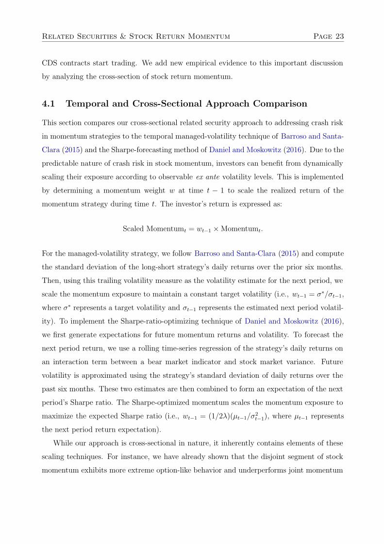
4.1 Temporal and Cross-Sectional Approach Comparison
This section compares our cross-sectional related security approach to addressing crash risk
in momentum strategies to the temporal managed-volatility technique of Barroso and Santa-
Clara (2015) and the Sharpe-forecasting method of Daniel and Moskowitz (2016). Due to the
predictable nature of crash risk in stock momentum, investors can benefit from dynamically
scaling their exposure according to observable ex ante volatility levels. This is implemented
by determining a momentum weight w at time t − 1 to scale the realized return of the
momentum strategy during time t. The investor’s return is expressed as:
Scaled Momentumt = wt−1 × Momentumt.
For the managed-volatility strategy, we follow Barroso and Santa-Clara (2015) and compute
the standard deviation of the long-short strategy’s daily returns over the prior six months.
Then, using this trailing volatility measure as the volatility estimate for the next period, we
scale the momentum exposure to maintain a constant target volatility (i.e., wt−1 = σ∗/σt−1,
where σ∗ represents a target volatility and σt−1 represents the estimated next period volatil-
ity). To implement the Sharpe-ratio-optimizing technique of Daniel and Moskowitz (2016),
we first generate expectations for future momentum returns and volatility. To forecast the
next period return, we use a rolling time-series regression of the strategy’s daily returns on
an interaction term between a bear market indicator and stock market variance. Future
volatility is approximated using the strategy’s standard deviation of daily returns over the
past six months. These two estimates are then combined to form an expectation of the next
period’s Sharpe ratio. The Sharpe-optimized momentum scales the momentum exposure to
maximize the expected Sharpe ratio (i.e., wt−1 = (1/2λ)(µt−1/σ2t−1), where µt−1 represents
the next period return expectation).
While our approach is cross-sectional in nature, it inherently contains elements of these
scaling techniques. For instance, we have already shown that the disjoint segment of stock
momentum exhibits more extreme option-like behavior and underperforms joint momentum

Related Securities & Stock Return Momentum Page 24
especially during periods of heightened volatility (see Tables 7 and 8, respectively). In this
section, we examine whether these temporal scaling techniques explain our cross-sectional-
based hedged momentum results and whether our hedging strategy can be further improved
by applying these scaling techniques.
Table 10 shows a comparison of various plain and scaled momentum strategies.25 The ta-
ble reports both the sample period Sharpe ratio for each strategy and the Treynor and Black
(1973) appraisal ratio relative a comparison strategy. The first category, Traditional Stock
Momentum (UMD), confirms that the volatility-scaled and Sharpe-forecasted strategies sig-
nificantly enhance the traditional stock momentum strategy during our sample period from
2003 to 2015. The second category, Statically Hedged Joint Momentum, includes scaled vari-
ations of our static-hedged joint momentum strategy that is 50% invested in joint momentum
and 50% in a disjoint contrarian position. The plain strategy generates a Sharpe ratio of 1.04,
which is 27% higher than the best-performing scaled UMD strategy [= (1 .04 − 0.82)/0.82].
To achieve a similar Sharpe ratio, the Sharpe-forecasted UMD strategy would need to com-
bined with an orthogonal investment exhibiting a Sharpe ratio of 0.64 (=√
1.042 − 0.822),
which is represented by the appraisal ratio. Furthermore, we find that scaling the hedged
strategy significantly improves its performance. For instance, the volatility-scaled hedged
joint momentum strategy generates a Sharpe ratio of 1.31 with an appraisal of 0.80 with
respect to plain hedged joint momentum.
The last category in Table 10 shows the scaled variations of our Dynamically Hedged
Joint Momentum strategy that invests in scaled joint momentum but switches to scaled
hedged joint momentum only during periods of heightened volatility.26 We find a large
improvement in performance of our dynamically hedged strategy after scaling according to
its volatility, producing a Sharpe ratio of 1.61 and an appraisal ratio of 0.85 against the plain
strategy. Overall, these results suggest that despite any commonalities between the temporal
scaling approaches and our cross-sectional approach, each leads to distinct improvements
in the risk-return profile of the stock momentum strategy. Investors can enjoy enhanced
25Each scaled strategy targets an annualized volatility of 20%, which mimics that of our plain in-samplestock momentum strategy. Note, however, that while the choice of target volatility can either amplify ordampen the performance of the scaled strategy, it does not affect its Sharpe ratio or appraisal ratio.
26For this exercise, the high volatility indicator is triggered when either stock market or joint momentumvolatility becomes elevated.
Related Securities & Stock Return Momentum Page 25
risk-managed momentum strategy profits by considering both temporal and cross-sectional
hedging approaches.
5 Related Securities and the Cross-Section of Stock
Return Momentum: The International Evidence
In this section, we turn to a sample of international firms headquartered outside the U.S. to
perform an out-of-sample test on related security performance and the cross-section of stock
return momentum and compare the robustness of our momentum segmentation structure
across countries with high and low economic development. The international sample consists
of 1,267 non-U.S. firms from 49 countries. CDS data are from the Markit Group and equity
data are from Datastream.27
Table 11 presents alpha coefficients on an international four-factor model that includes
international (ex-U.S.) MKT , SMB, HML, and UMDS factors.28 Using a CDS formation
horizon of J = 4m, we find positive risk-adjusted returns on the joint stock/CDS momentum
strategy and a significant disparity in performance between joint and disjoint momentum.
Column 1 shows that joint momentum generates an alpha of 0.83% per month with a t-
statistic of 2.69 and Sharpe ratio of 0.55. In column 2 we see that disjoint momentum
produces a negative alpha of -0.28% per month (t-statistic of -2.70). An international stat-
ically hedged joint momentum portfolio that invests 50% in international joint momentum
while hedging with 50% in a disjoint contrarian strategy generates a statistically significant
0.55% per month with a t-statistic of 2.72 and Sharpe ratio of 0.87. The dynamically hedged
joint momentum strategy that switches from joint momentum to a hedged strategy during
high volatility periods generates 1.21% per month with a t-statistic of 4.03 and Sharpe ratio
of 1.05.29 These international results confirm our earlier findings that CDS performance
information is important in explaining the cross-section of stock momentum.
27Similar to our filters on the U.S. sample, we require firms’ equity market capitalization to be greaterthan $100 million (USD) at the time of portfolio formation and for the CDS to have no more than 10%missing observations and no more than 90% stagnant observations over the prior six months.
28See Ken French’s site (http://mba.tuck.dartmouth.edu/pages/faculty/ken.french/data library.html) forthe international (ex-U.S.) MKT , SMB, and HML.
29The high volatility indicator equals one when the two-year change in trailing market volatility is greaterthan zero.

Related Securities & Stock Return Momentum Page 26
Next, we separate countries by high and low economic development and repeat our analy-
sis. In Section 3.4 we provided a relative pricing framework for our momentum segmentation
results and in Table 6 showed that the underperformance of disjoint momentum appears to
closely related to arbitrageurs acting on mispricing between stock and CDS markets. Because
the stock market segmentation concept of Goldstein, Li, and Yang (2014) is most applicable
when there exists a relatively wider variety of trading motives among stock market investors,
we hypothesize that the joint-disjoint performance differential is greatest among more de-
veloped economies that are populated with a greater number of sophisticated hedgers (i.e.,
cross-market arbitrageurs) in proportion to speculators (i.e., momentum traders).
The international sample is divided into two roughly equally-sized groups based on GDP-
per-capita, assigning 633 firms to the more developed group (high GDP-per-capita) and 634
firms to the less developed group (low GDP-per-capita). International four-factor alpha
coefficients for these two groups are presented in Table 11. We find that joint momentum
performance (column 1) is much greater in the sample of more developed countries, generat-
ing an alpha of 1.15% per month (t-statistic of 3.35 and Sharpe ratio of 0.55), compared to
the statistically insignificant 0.38% per month among less developed countries. Similarly, the
underperformance of disjoint momentum (column 2) is exacerbated in the sample of more
developed countries (-0.40% per month) relative to that of less developed countries (-0.07%
per month).
We also find the performance differential between joint and disjoint momentum to be
much wider and statistically significant only in the sample of more developed countries. The
statically hedged joint momentum strategy (column 3) that maintains a constant 50% in
joint momentum and 50% in a disjoint contrarian strategy generates an alpha of 0.78% per
month among the more developed countries (t-statistic of 3.11 and Sharpe ratio of 0.83) and
only 0.22% per month among the less developed countries (t-statistic of 0.84 and Sharpe
ratio of 0.37). The dynamically hedged joint momentum strategy (column 4) proves to
be nearly twice as profitable among more developed countries in relation to less developed
countries (1.47% per month versus 0.82% per month, respectively) and has greater statistical
significance (t-statistic of 3.72 versus 2.38). These findings are closely related to Jacobs
(2016) who shows that mispricing-based stock market anomalies appear to be at least as
profitable in developed markets as in developing markets.
Related Securities & Stock Return Momentum Page 27
Figure 7 displays the cumulative profits from an global strategy (50% U.S., 50% Non-U.S.)
that uses related security performance information to dynamically hedge risk and improve
the performance of traditional stock momentum. The global dynamic hedging strategy
exhibits a Sharpe ratio of 1.55, which represents a vast improvement over the 0.13 of the
depicted global stock momentum strategy. Put together, our international findings further
solidify the robustness of our baseline results and provide further evidence that cross-market
arbitrage plays an important role in explaining why related security performance matters in
the cross-section of stock momentum.
6 Conclusion
We introduce a simple yet powerful approach to detect relative underreaction and over-
valuation in stock prices to underlying firm fundamentals using related security prices. In
particular, we focus on single-name CDS contracts as related securities. When pricing signals
are extended to include related CDS pricing information, we sharply identify the cross-section
of stocks that are underreacting to firm fundamentals – thereby showing subsequent price
momentum. Further, we are able to detect which stocks are likely to show price reversal due,
in part, to strong convergence pressure on their share prices arising from misaligned equity
and credit security prices.
Using 881 U.S. public firms that have actively trading five-year maturity single name
CDS contracts during 2003-2015, we document the following important differences in the
cross-section of stock return momentum. First, we show that segmenting traditional stock
momentum (Jegadeesh and Titman, 1993) based on the degree of cross-sectional past per-
formance ranking agreement between stock and CDS markets reveals a stark contrast in
momentum strategy returns. In particular, joint entities that have strong agreement in
past performance exhibit a much stronger momentum effect than disjoint entities with dis-
agreement in past stock and CDS performance. The performance differential between these
joint and disjoint components of stock momentum exceeds 20% per year. This finding is
consistent with the notion of Goldstein, Li, and Yang (2014) that stock markets may be
segmented with momentum traders and contrarian hedgers whose trades are motivated by
relative pricing between stock and CDS markets. That is, under a relative pricing frame-
Related Securities & Stock Return Momentum Page 28
work, the underperformance of disjoint momentum can be explained in part by cross-market
arbitrageurs acting on disjoint stocks that misprice underlying credit risks relative to the
CDS. We further observe that disjoint momentum is more sensitive to momentum crash risk
during bear market rebounds (Daniel and Moskowitz, 2016) and underperforms joint mo-
mentum especially during periods of high volatility. Based on these observations, we present
various hedging strategies that eliminate crash risk and significantly improve the risk-return
profile of the traditional stock momentum strategy, providing an alpha of up to 18% per
year and a Sharpe ratio of 1.37. As an additional out-of-sample robustness test, we extend
our findings to 1,267 international firms from 49 countries.
Overall, we provide several important contributions to three relevant research streams.
First, we show that related security pricing information is important in identifying individual
stock momentum cycles (Lee and Swaminathan, 2000) through a relative pricing framework
(Schaefer and Strebulaev, 2008; Friewald, Wagner, and Zechner, 2014; Bai and Wu, 2016;
Yu, 2006; Duarte, Longstaff, and Yu, 2007; Kapadia and Pu, 2012). Second, we provide a
novel cross-sectional approach to detect a group of stocks that are more prone to momen-
tum crashes (Daniel and Moskowitz, 2016; Daniel, Jagannathan, and Kim, 2012; Grundy
and Martin, 2001; Barroso and Santa-Clara, 2015; Han, Zhou, and Zhu, 2016). Third, our
results contribute evidence on the recent notion that related securities induce stock market
segmentation, which, in turn, can reduce stock price efficiency and cause excess volatility
(Goldstein, Li, and Yang, 2014; Boehmer, Chava, and Tookes, 2016).
Our results shed new light on interactive cross-market anomalies rooted in market seg-
mentation. We show how a firm’s capital structure serves as a bridge for trading activity
between stock and CDS markets, providing an explanation for why one might observe seg-
mentation within the U.S. stock market. Given the complexity and increasing connectedness
of global capital markets, other cross-asset, cross-market trading networks could further ex-
plain market segmentation structures (i.e., the relative volatility pricing between stock op-
tions and CDS markets, cross-country equity and credit market integration networks, among
others). Identifying such interactive trading networks improves our understanding of asset
pricing dynamics and market efficiency.

Related Securities & Stock Return Momentum Page 29
References
Acharya, Viral V., and Timothy C. Johnson, 2007, Insider trading in credit derivatives,
Journal of Financial Economics 84, 110–141.
An, Byeong-Je, Andrew Ang, Turan G Bali, and Nusret Cakici, 2014, The joint cross section
of stocks and options, The Journal of Finance 69, 2279–2337.
Asness, Clifford S., Andrea Frazzini, and Lasse H. Pedersen, 2014, Quality minus junk, New
York University Working Paper.
Asness, Clifford S., Tobias J. Moskowitz, and Lasse Heje Pedersen, 2013, Value and momen-
tum everywhere, The Journal of Finance 68, 929–985.
Avramov, Doron, Tarun Chordia, Gergana Jostova, and Alexander Philipov, 2009, Credit
ratings and the cross-section of stock returns, Journal of Financial Markets 12, 469–499.
Bai, Jennie, and Liuren Wu, 2016, Anchoring corporate credit spreads to firm fundamentals,
Journal of Financial and Quantitative Analysis, forthcoming.
Barroso, Pedro, and Pedro Santa-Clara, 2015, Momentum has its moments, Journal of Fi-
nancial Economics 116, 111–120.
Batta, George E, Jiaping Qiu, and Fan Yu, 2016, Credit derivatives and analyst behavior,
The Accounting Review 91, 1315–1343.
Berndt, Antje, and Iulian Obreja, 2010, Decomposing European CDS returns, Review of
Finance 14, 189–233.
Boehmer, Ekkehart, Sudheer Chava, and Heather Tookes, 2016, Related securities and equity
market quality: The case of cds, Journal of Financial and Quantitative Analysis 50, 509–
541.
Campbell, John Y, Jens Hilscher, and Jan Szilagyi, 2008, In search of distress risk, The
Journal of Finance 63, 2899–2939.
Carhart, Mark M, 1997, On persistence in mutual fund performance, The Journal of finance
52, 57–82.

Related Securities & Stock Return Momentum Page 30
Chava, Sudheer, Rohan Ganduri, and Chayawat Ornthanalai, 2012, Are credit ratings still
relevant?, Working Paper, Georgia Institute of Technology and University of Toronto.
Cooper, Michael J, Roberto C Gutierrez, and Allaudeen Hameed, 2004, Market states and
momentum, The Journal of Finance 59, 1345–1365.
Daniel, Kent, Ravi Jagannathan, and Soohun Kim, 2012, Tail risk in momentum strategy
returns, Working Paper, Columbia University and Northwestern University.
Daniel, Kent, and Tobias Moskowitz, 2016, Momentum crashes, Journal of Financial Eco-
nomics, forthcoming.
Dichev, Ilia D, 1998, Is the risk of bankruptcy a systematic risk?, The Journal of Finance
53, 1131–1147.
Duarte, Jefferson, Francis A Longstaff, and Fan Yu, 2007, Risk and return in fixed-income
arbitrage: Nickels in front of a steamroller?, Review of Financial Studies 20, 769–811.
Fama, Eugene F, and Kenneth R French, 1993, Common risk factors in the returns on stocks
and bonds, Journal of Financial Economics 33, 3–56.
Flannery, Mark, Joel Houston, and Frank Partnoy, 2010, Credit default swap spreads as
viable substitutes for credit ratings, University of Pennsylvania Law Review 158, 10–031.
Friewald, Nils, Christian Wagner, and Josef Zechner, 2014, The cross-section of credit risk
premia and equity returns, The Journal of Finance 69, 2419–2469.
Gebhardt, William R, Soeren Hvidkjaer, and Bhaskaran Swaminathan, 2005, The cross-
section of expected corporate bond returns: Betas or characteristics?, Journal of Financial
Economics 75, 85–114.
Goldstein, Itay, Yan Li, and Liyan Yang, 2014, Speculation and hedging in segmented mar-
kets, Review of Financial Studies 27, 881–922.
Grundy, Bruce D, and J Spencer Martin, 2001, Understanding the nature of the risks and
the source of the rewards to momentum investing, Review of Financial Studies 14, 29–78.
Related Securities & Stock Return Momentum Page 31
Han, Bing, Avanidhar Subrahmanyam, and Yi Zhou, 2016, The term structure of credit
spreads and the cross-section of stock returns, Journal of Financial Economics, forthcom-
ing.
Han, Yufeng, Guofu Zhou, and Yingzi Zhu, 2016, Taming momentum crashes: A simple
stop-loss strategy, Working Paper, University of North Carolina at Charlotte, Washington
University in St. Louis, and Tsinghua University.
Hull, John, Mirela Predescu, and Alan White, 2004, The relationship between credit default
swap spreads, bond yields, and credit rating announcements, Journal of Banking and
Finance 28, 2789–2811.
Jacobs, Heiko, 2016, Market maturity and mispricing, Journal of Financial Economics,
forthcoming.
Jegadeesh, Narasimhan, and Sheridan Titman, 1993, Returns to buying winners and selling
losers: Implications for stock market efficiency, The Journal of Finance 48, 65–91.
Jostova, Gergana, Stanislava Nikolova, Alexander Philipov, and Christof W Stahel, 2013,
Momentum in corporate bond returns, Review of Financial Studies 26, 1649–1693.
Kapadia, Nikunj, and Xiaoling Pu, 2012, Limited arbitrage between equity and credit mar-
kets, Journal of Financial Economics 105, 542–564.
Kisgen, Darren J., 2006, Credit ratings and capital structure, The Journal of Finance 61,
1035–1072.
, 2007, The influence of credit ratings on corporate capital structure decisions, Journal
of Applied Corporate Finance 19, 65–73.
Lee, Charles, and Bhaskaran Swaminathan, 2000, Price momentum and trading volume, The
Journal of Finance 55, 2017–2069.
Lee, Jongsub, Andy Naranjo, and Stace Sirmans, 2014, CDS momentum: Slow moving credit
ratings and cross-market spillovers, Working Paper, University of Arkansas and University
of Florida.
Related Securities & Stock Return Momentum Page 32
Merton, Robert C., 1974, On the pricing of corporate debt: The risk structure of interest
rates, The Journal of Finance 29, 449–470.
Nelson, Charles R., and Andrew F. Siegel, 1987, Parsimonious modeling of yield curves,
Journal of Business 60, 473–489.
Ni, Sophie, and Jun Pan, 2010, Trading puts and CDS on stocks with short sale ban, Working
Paper, Hong Kong University and MIT.
Novy-Marx, Robert, 2012, Is momentum really momentum?, Journal of Financial Economics
103, 429–453.
, 2013, The other side of value: The gross profitability premium, Journal of Financial
Economics 108, 1–28.
, 2015, Fundamentally, momentum is fundamental momentum, Working Paper, Uni-
versity of Rochester.
O’Kane, Dominic, 2008, Modelling Single-name and Multi-name Credit Derivatives (John
Wiley & Sons).
Pastor, Lubos, and Robert F. Stambaugh, 2003, Liquidity risk and expected stock returns,
Journal of Political Economy 111, 642–685.
Qiu, Jiaping, and Fan Yu, 2012, Endogenous liquidity in credit derivatives, Journal of Fi-
nancial Economics 103, 611–631.
Schaefer, Stephen M, and Ilya A Strebulaev, 2008, Structural models of credit risk are useful:
Evidence from hedge ratios on corporate bonds, Journal of Financial Economics 90, 1–19.
Stambaugh, Robert F., and Yu Yuan, 2016, Mispricing factors, Review of Financial Studies,
forthcoming.
Svensson, Lars, 1994, Estimating and interpreting forward interest rates: Sweden 1992-1994,
Centre for Economic Policy Research, Discussion Paper 1051.
Treynor, Jack L., and Fischer Black, 1973, How to use security analysis to improve portfolio
selection, Journal of Business 46, 66–86.

Related Securities & Stock Return Momentum Page 33
Yu, Fan, 2006, How profitable is capital structure arbitrage?, Financial Analysts Journal 62,
47–62.
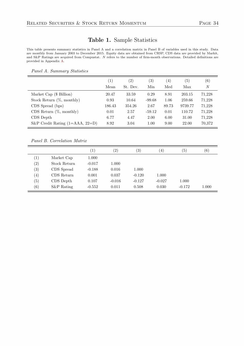
Related Securities & Stock Return Momentum Page 34
Table 1. Sample Statistics
This table presents summary statistics in Panel A and a correlation matrix in Panel B of variables used in this study. Dataare monthly from January 2003 to December 2015. Equity data are obtained from CRSP, CDS data are provided by Markit,and S&P Ratings are acquired from Compustat. N refers to the number of firm-month observations. Detailed definitions areprovided in Appendix A.
Panel A. Summary Statistics
(1) (2) (3) (4) (5) (6)Mean St. Dev. Min Med Max N
Market Cap ($ Billion) 20.47 33.59 0.29 8.91 203.15 71,228Stock Return (%, monthly) 0.93 10.64 -99.68 1.06 259.66 71,228CDS Spread (bps) 186.43 354.26 2.67 89.73 9739.77 71,228CDS Return (%, monthly) 0.01 2.57 -59.12 0.01 110.72 71,228CDS Depth 6.77 4.47 2.00 6.00 31.00 71,228S&P Credit Rating (1=AAA, 22=D) 8.92 3.04 1.00 9.00 22.00 70,372
Panel B. Correlation Matrix
(1) (2) (3) (4) (5) (6)
(1) Market Cap 1.000(2) Stock Return -0.017 1.000(3) CDS Spread -0.188 0.016 1.000(4) CDS Return 0.001 0.037 -0.120 1.000(5) CDS Depth 0.107 -0.016 -0.127 -0.027 1.000(6) S&P Rating -0.552 0.011 0.508 0.030 -0.172 1.000

Related Securities & Stock Return Momentum Page 35
Table 2. Joint Stock/CDS Market Momentum
This table presents our joint stock/CDS momentum results. The joint winner and loser portfolios, JW and JL, respectively, aredefined as the overlap between stock momentum portfolios and CDS momentum portfolios. We denote stock losers (winners)by LS (WS) and CDS losers (winners) by LC (WC). Stock momentum portfolios are based on quintiles of the past 12-monthstock return, skipping the most recent month. CDS momentum portfolios are based on quintiles of the past J-month CDSreturn, where J ranges from from 1 to 12 months. The holding period is one month (K = 1). We segment the traditional stockmomentum strategy into two parts based on the overlap between stock and CDS winner and loser portfolios as follows:
Stock Momentum ≡ (WS − LS)
⎧⎨
⎩
Joint Stock/CDS Momentum ≡ (WS ∩ WC) − (LS ∩ LC)
Disjoint Stock/CDS Momentum ≡ (WS \ WC) − (LS \ LC).
The “4-factor” model includes MKT , SMB, HML, and our in-sample stock momentum factor, UMDS . The UMDS factor isconstructed in-sample using quintiles of firms’ past 12-month stock return (J = 12m), skipping the most recent month, and aholding period of one month (K = 1m). Percentage returns are monthly and span the time period January 2003 to December2015. The 12-lag Newey-West t-statistic is provided in parenthesis, and ∗, ∗∗, and ∗∗∗ are indicators of statistical significanceat the 10%, 5%, and 1% levels, respectively. Notation for each portfolio return follows the pattern: mean, ( t-statistic), andannualized Sharpe ratio.
Joint Stock/CDS Momentum Momentum Segmentation
(1) (2) (3) (4) (5) (6) (7)JL ≡ JW ≡ Joint ≡ Joint Joint – Disjoint – Joint –
LS∩LC WS∩WC JW-JL 4-factor α (WS-LS) (WS-LS) Disjoint
J = 1m 0.20 1.46∗∗∗ 1.25∗ 1.00∗∗∗ 0.95∗∗∗ -0.34∗∗∗ 1.29∗∗∗(0.23) (2.82) (1.79) (2.92) (2.68) (-2.77) (2.98)0.08 0.84 0.57 0.73 -0.91 0.84
J = 2m 0.17 1.29∗∗ 1.12∗ 0.86∗∗ 0.82∗∗ -0.35∗∗∗ 1.17∗∗∗(0.20) (2.52) (1.66) (2.56) (2.27) (-3.52) (2.73)0.07 0.82 0.54 0.74 -0.98 0.85
J = 3m 0.082 1.22∗∗ 1.13∗∗ 0.85∗∗∗ 0.83∗∗∗ -0.16 0.98∗∗∗(0.09) (2.17) (2.14) (2.94) (3.40) (-1.14) (2.93)0.04 0.71 0.57 0.66 -0.35 0.65
J = 4m -0.15 1.49∗∗∗ 1.64∗∗∗ 1.45∗∗∗ 1.34∗∗∗ -0.39∗∗∗ 1.73∗∗∗(-0.16) (2.69) (2.83) (4.24) (4.08) (-2.71) (3.94)-0.06 0.88 0.81 1.05 -0.79 1.04
J = 5m -0.18 1.31∗∗ 1.49∗∗ 1.25∗∗∗ 1.19∗∗∗ -0.34∗∗∗ 1.52∗∗∗(-0.21) (2.33) (2.56) (3.83) (3.61) (-2.86) (3.57)-0.08 0.78 0.75 1.02 -0.76 1.02
J = 6m 0.11 1.24∗∗ 1.14∗ 0.91∗∗ 0.83∗∗ -0.27∗∗ 1.10∗∗(0.13) (2.40) (1.66) (2.60) (2.22) (-2.14) (2.28)0.05 0.79 0.54 0.75 -0.64 0.76
J = 9m -0.085 1.20∗∗∗ 1.29∗ 1.04∗∗∗ 0.98∗∗∗ -0.37∗ 1.35∗∗(-0.09) (2.66) (1.82) (3.26) (2.72) (-1.85) (2.49)-0.04 0.78 0.61 0.92 -0.68 0.88
J = 12m 0.062 1.10∗∗∗ 1.04 0.72∗∗ 0.74∗∗ -0.34∗ 1.08∗∗(0.07) (2.61) (1.54) (2.40) (2.32) (-1.73) (2.16)0.03 0.71 0.51 0.78 -0.62 0.77
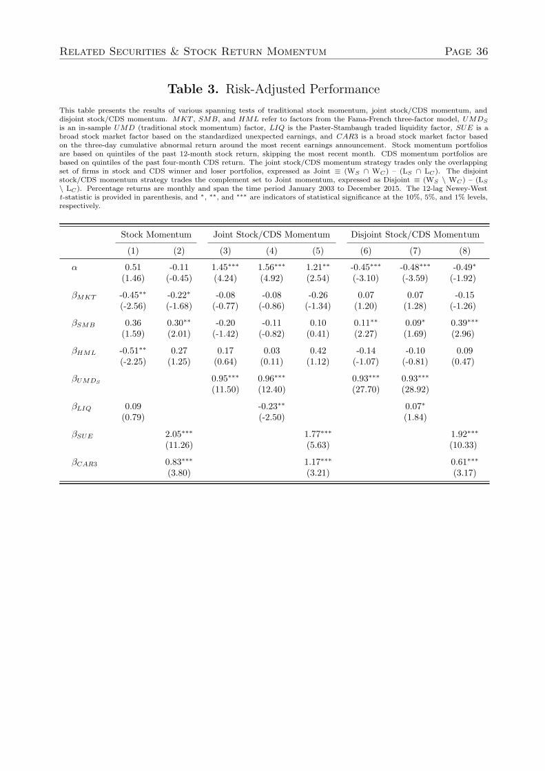
Related Securities & Stock Return Momentum Page 36
Table 3. Risk-Adjusted Performance
This table presents the results of various spanning tests of traditional stock momentum, joint stock/CDS momentum, anddisjoint stock/CDS momentum. MKT , SMB, and HML refer to factors from the Fama-French three-factor model, UMDS
is an in-sample UMD (traditional stock momentum) factor, LIQ is the Paster-Stambaugh traded liquidity factor, SUE is abroad stock market factor based on the standardized unexpected earnings, and CAR3 is a broad stock market factor basedon the three-day cumulative abnormal return around the most recent earnings announcement. Stock momentum portfoliosare based on quintiles of the past 12-month stock return, skipping the most recent month. CDS momentum portfolios arebased on quintiles of the past four-month CDS return. The joint stock/CDS momentum strategy trades only the overlappingset of firms in stock and CDS winner and loser portfolios, expressed as Joint ≡ (WS ∩ WC) – (LS ∩ LC). The disjointstock/CDS momentum strategy trades the complement set to Joint momentum, expressed as Disjoint ≡ (WS \ WC) – (LS
\ LC). Percentage returns are monthly and span the time period January 2003 to December 2015. The 12-lag Newey-Westt-statistic is provided in parenthesis, and ∗, ∗∗, and ∗∗∗ are indicators of statistical significance at the 10%, 5%, and 1% levels,respectively.
Stock Momentum Joint Stock/CDS Momentum Disjoint Stock/CDS Momentum
(1) (2) (3) (4) (5) (6) (7) (8)
α 0.51 -0.11 1.45∗∗∗ 1.56∗∗∗ 1.21∗∗ -0.45∗∗∗ -0.48∗∗∗ -0.49∗(1.46) (-0.45) (4.24) (4.92) (2.54) (-3.10) (-3.59) (-1.92)
βMKT -0.45∗∗ -0.22∗ -0.08 -0.08 -0.26 0.07 0.07 -0.15(-2.56) (-1.68) (-0.77) (-0.86) (-1.34) (1.20) (1.28) (-1.26)
βSMB 0.36 0.30∗∗ -0.20 -0.11 0.10 0.11∗∗ 0.09∗ 0.39∗∗∗(1.59) (2.01) (-1.42) (-0.82) (0.41) (2.27) (1.69) (2.96)
βHML -0.51∗∗ 0.27 0.17 0.03 0.42 -0.14 -0.10 0.09(-2.25) (1.25) (0.64) (0.11) (1.12) (-1.07) (-0.81) (0.47)
βUMDS 0.95∗∗∗ 0.96∗∗∗ 0.93∗∗∗ 0.93∗∗∗(11.50) (12.40) (27.70) (28.92)
βLIQ 0.09 -0.23∗∗ 0.07∗(0.79) (-2.50) (1.84)
βSUE 2.05∗∗∗ 1.77∗∗∗ 1.92∗∗∗(11.26) (5.63) (10.33)
βCAR3 0.83∗∗∗ 1.17∗∗∗ 0.61∗∗∗(3.80) (3.21) (3.17)
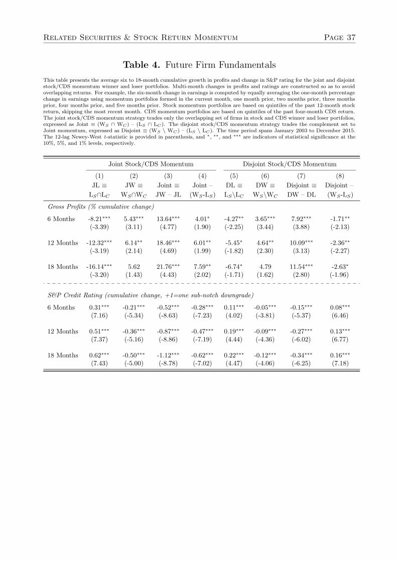
Related Securities & Stock Return Momentum Page 37
Table 4. Future Firm Fundamentals
This table presents the average six to 18-month cumulative growth in profits and change in S&P rating for the joint and disjointstock/CDS momentum winner and loser portfolios. Multi-month changes in profits and ratings are constructed so as to avoidoverlapping returns. For example, the six-month change in earnings is computed by equally averaging the one-month percentagechange in earnings using momentum portfolios formed in the current month, one month prior, two months prior, three monthsprior, four months prior, and five months prior. Stock momentum portfolios are based on quintiles of the past 12-month stockreturn, skipping the most recent month. CDS momentum portfolios are based on quintiles of the past four-month CDS return.The joint stock/CDS momentum strategy trades only the overlapping set of firms in stock and CDS winner and loser portfolios,expressed as Joint ≡ (WS ∩ WC) – (LS ∩ LC). The disjoint stock/CDS momentum strategy trades the complement set toJoint momentum, expressed as Disjoint ≡ (WS \ WC) – (LS \ LC). The time period spans January 2003 to December 2015.The 12-lag Newey-West t-statistic is provided in parenthesis, and ∗, ∗∗, and ∗∗∗ are indicators of statistical significance at the10%, 5%, and 1% levels, respectively.
Joint Stock/CDS Momentum Disjoint Stock/CDS Momentum
(1) (2) (3) (4) (5) (6) (7) (8)JL ≡ JW ≡ Joint ≡ Joint – DL ≡ DW ≡ Disjoint ≡ Disjoint –
LS∩LC WS∩WC JW – JL (WS-LS) LS\LC WS\WC DW – DL (WS-LS)
Gross Profits (% cumulative change)
6 Months -8.21∗∗∗ 5.43∗∗∗ 13.64∗∗∗ 4.01∗ -4.27∗∗ 3.65∗∗∗ 7.92∗∗∗ -1.71∗∗(-3.39) (3.11) (4.77) (1.90) (-2.25) (3.44) (3.88) (-2.13)
12 Months -12.32∗∗∗ 6.14∗∗ 18.46∗∗∗ 6.01∗∗ -5.45∗ 4.64∗∗ 10.09∗∗∗ -2.36∗∗(-3.19) (2.14) (4.69) (1.99) (-1.82) (2.30) (3.13) (-2.27)
18 Months -16.14∗∗∗ 5.62 21.76∗∗∗ 7.59∗∗ -6.74∗ 4.79 11.54∗∗∗ -2.63∗(-3.20) (1.43) (4.43) (2.02) (-1.71) (1.62) (2.80) (-1.96)
S&P Credit Rating (cumulative change, +1=one sub-notch downgrade)
6 Months 0.31∗∗∗ -0.21∗∗∗ -0.52∗∗∗ -0.28∗∗∗ 0.11∗∗∗ -0.05∗∗∗ -0.15∗∗∗ 0.08∗∗∗(7.16) (-5.34) (-8.63) (-7.23) (4.02) (-3.81) (-5.37) (6.46)
12 Months 0.51∗∗∗ -0.36∗∗∗ -0.87∗∗∗ -0.47∗∗∗ 0.19∗∗∗ -0.09∗∗∗ -0.27∗∗∗ 0.13∗∗∗(7.37) (-5.16) (-8.86) (-7.19) (4.44) (-4.36) (-6.02) (6.77)
18 Months 0.62∗∗∗ -0.50∗∗∗ -1.12∗∗∗ -0.62∗∗∗ 0.22∗∗∗ -0.12∗∗∗ -0.34∗∗∗ 0.16∗∗∗(7.43) (-5.00) (-8.78) (-7.02) (4.47) (-4.06) (-6.25) (7.18)
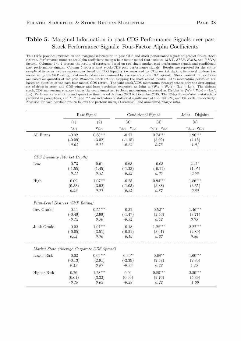
Related Securities & Stock Return Momentum Page 38
Table 5. Marginal Information in past CDS Performance Signals over pastStock Performance Signals: Four-Factor Alpha Coefficients
This table provides evidence on the marginal information in past CDS and stock performance signals to predict future stockreturns. Performance numbers are alpha coefficients using a four-factor model that includes MKT , SMB, HML, and UMDS
factors. Columns 1 to 4 present the results of strategies based on raw single-market past performance signals and conditionalpast performance signals. Column 5 reports joint stock/CDS past performance signals. Results are reported for the entiresample of firms as well as sub-samples based on CDS liquidity (as measured by CDS market depth), firm-level distress (asmeasured by the S&P rating), and market state (as measured by average corporate CDS spread). Stock momentum portfoliosare based on quintiles of the past 12-month stock return, skipping the most recent month. CDS momentum portfolios arebased on quintiles of the past four-month CDS return. The joint stock/CDS momentum strategy trades only the overlappingset of firms in stock and CDS winner and loser portfolios, expressed as Joint ≡ (WS ∩ WC) – (LS ∩ LC). The disjointstock/CDS momentum strategy trades the complement set to Joint momentum, expressed as Disjoint ≡ (WS \ WC) – (LS \LC). Performance is monthly and spans the time period January 2003 to December 2015. The 12-lag Newey-West t-statistic isprovided in parenthesis, and ∗, ∗∗, and ∗∗∗ are indicators of statistical significance at the 10%, 5%, and 1% levels, respectively.Notation for each portfolio return follows the pattern: mean, (t-statistic), and annualized Sharpe ratio.
Raw Signal Conditional Signal Joint – Disjoint
(1) (2) (3) (4) (5)rS,4 rC,4 rS,4 | rC,4 rC,4 | rS,4 rS,12, rC,4
All Firms -0.02 0.88∗∗∗ -0.27 0.74∗∗∗ 1.90∗∗∗(-0.09) (3.02) (-1.15) (3.02) (4.15)-0.04 0.71 -0.29 0.75 1.04
CDS Liquidity (Market Depth)
Low -0.73 0.61 -0.63 -0.03 2.41∗(-1.55) (1.45) (-1.23) (-0.11) (1.95)-0.41 0.34 -0.39 0.05 0.58
High 0.09 1.07∗∗∗ -0.25 0.94∗∗∗ 1.86∗∗∗(0.38) (3.92) (-1.03) (3.88) (3.65)0.02 0.77 -0.25 0.87 0.85
Firm-Level Distress (S&P Rating)
Inv. Grade -0.11 0.55∗∗∗ -0.32 0.52∗∗ 1.46∗∗∗(-0.49) (2.99) (-1.47) (2.46) (3.71)-0.12 0.50 -0.34 0.52 0.75
Junk Grade -0.02 1.07∗∗∗ -0.18 1.28∗∗∗ 2.22∗∗∗(-0.05) (3.51) (-0.51) (3.61) (2.89)0.04 0.70 -0.10 0.97 0.80
Market State (Average Corporate CDS Spread)
Lower Risk -0.02 0.69∗∗∗ -0.39∗∗ 0.68∗∗ 1.60∗∗∗(-0.13) (2.91) (-2.39) (2.58) (2.80)0.19 0.87 -0.33 0.82 1.13
Higher Risk 0.26 1.28∗∗∗ 0.04 0.80∗∗∗ 2.59∗∗∗(0.61) (3.32) (0.09) (2.76) (5.39)-0.19 0.62 -0.28 0.72 1.00
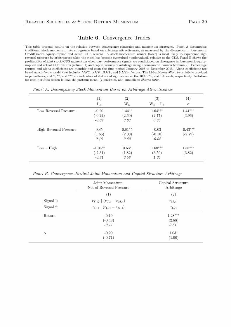
Related Securities & Stock Return Momentum Page 39
Table 6. Convergence Trades
This table presents results on the relation between convergence strategies and momentum strategies. Panel A decomposestraditional stock momentum into sub-groups based on arbitrage attractiveness, as measured by the divergence in four-monthCreditGrades equity-implied and actual CDS returns. A stock momentum winner (loser) is most likely to experience highreversal pressure by arbitrageurs when the stock has become overvalued (undervalued) relative to the CDS. Panel B shows theprofitability of joint stock/CDS momentum when past performance signals are conditioned on divergence in four-month equity-implied and actual CDS returns (column 1) and capital structure arbitrage using a four-month horizon (column 2). Percentagereturns and alpha coefficients are monthly and span the time period January 2003 to December 2015. Alpha coefficients arebased on a 4-factor model that includes MKT , SMB, HML, and UMDS factors. The 12-lag Newey-West t-statistic is providedin parenthesis, and ∗, ∗∗, and ∗∗∗ are indicators of statistical significance at the 10%, 5%, and 1% levels, respectively. Notationfor each portfolio return follows the pattern: mean, (t-statistic), and annualized Sharpe ratio.
Panel A. Decomposing Stock Momentum Based on Arbitrage Attractiveness
(1) (2) (3) (4)LS WS WS – LS α
Low Reversal Pressure -0.20 1.44∗∗ 1.64∗∗∗ 1.44∗∗∗(-0.22) (2.60) (2.77) (3.96)-0.09 0.87 0.85
High Reversal Pressure 0.85 0.81∗∗ -0.03 -0.43∗∗∗(1.65) (2.00) (-0.10) (-2.79)0.48 0.62 -0.02
Low – High -1.05∗∗ 0.63∗ 1.68∗∗∗ 1.88∗∗∗(-2.31) (1.82) (3.59) (3.82)-0.91 0.58 1.05
Panel B. Convergence-Neutral Joint Momentum and Capital Structure Arbitrage
Joint Momentum, Capital StructureNet of Reversal Pressure Arbitrage
(1) (2)
Signal 1: rS,12 | (rC,4 − rM,4) rM,4
Signal 2: rC,4 | (rC,4 − rM,4) rC,4
Return -0.19 1.28∗∗∗(-0.48) (2.88)-0.11 0.61
α -0.29 1.03∗(-0.71) (1.90)

Related Securities & Stock Return Momentum Page 40
Table 7. Time-Varying Beta and Option-Like Payoff Risk of Joint and Dis-joint Stock/CDS Momentum Strategies
This table presents results of time-series regressions of joint and disjoint stock/CDS momentum strategy returns. The inde-pendent variables include a bear market indicator that equals one when the two-year lagging market return is negative (IB),the market return (MKT), an interaction term between the market return and a bear market indicator (MKT×IB), and aninteraction term between the market return, a bear market indicator, and a contemporaneous up-market indicator that equalsone when the current month market return is positive (MKT×IB×IU ). Stock momentum portfolios are based on quintiles ofthe past 12-month stock return, skipping the most recent month. CDS momentum portfolios are based on quintiles of the pastfour-month CDS return. The joint stock/CDS momentum strategy trades only the overlapping set of firms in stock and CDSwinner and loser portfolios, expressed as Joint ≡ (WS ∩ WC) – (LS ∩ LC). The disjoint stock/CDS momentum strategy tradesthe complement set to Joint momentum, expressed as Disjoint ≡ (WS \ WC) – (LS \ LC). Performance is monthly and spansthe time period January 2003 to December 2015. The 12-lag Newey-West t-statistic is provided in parenthesis, and ∗, ∗∗, and∗∗∗ are indicators of statistical significance at the 10%, 5%, and 1% levels, respectively.
(1) (2) (3) (4)
Joint Stock/CDS Momentum ≡ (WS ∩ WC) – (LS ∩ LC)
α0 2.03∗∗∗ 2.38∗∗∗ 2.38∗∗∗ 2.28∗∗∗(3.96) (4.13) (4.12) (4.29)
αIB -2.07∗ -1.42(-1.69) (-0.72)
βMKT -0.53∗∗ -0.40∗ -0.40∗ -0.39∗(-2.48) (-1.88) (-1.88) (-1.87)
βMKT×IB -0.29 -0.19 -0.056(-0.80) (-0.42) (-0.14)
βMKT×IB×IU -0.24 -0.59(-0.30) (-1.30)
Disjoint Stock/CDS Momentum ≡ (WS \ WC) – (LS \ LC)
α0 0.18 0.41 0.41 0.55(0.65) (1.23) (1.22) (1.58)
αIB -1.86∗∗ 1.93(-2.14) (1.17)
βMKT -0.36 -0.11 -0.11 -0.12(-1.59) (-0.82) (-0.81) (-0.90)
βMKT×IB -0.53 0.049 -0.13(-1.54) (0.20) (-0.53)
βMKT×IB×IU -1.40∗∗ -0.92∗∗∗(-2.41) (-2.88)
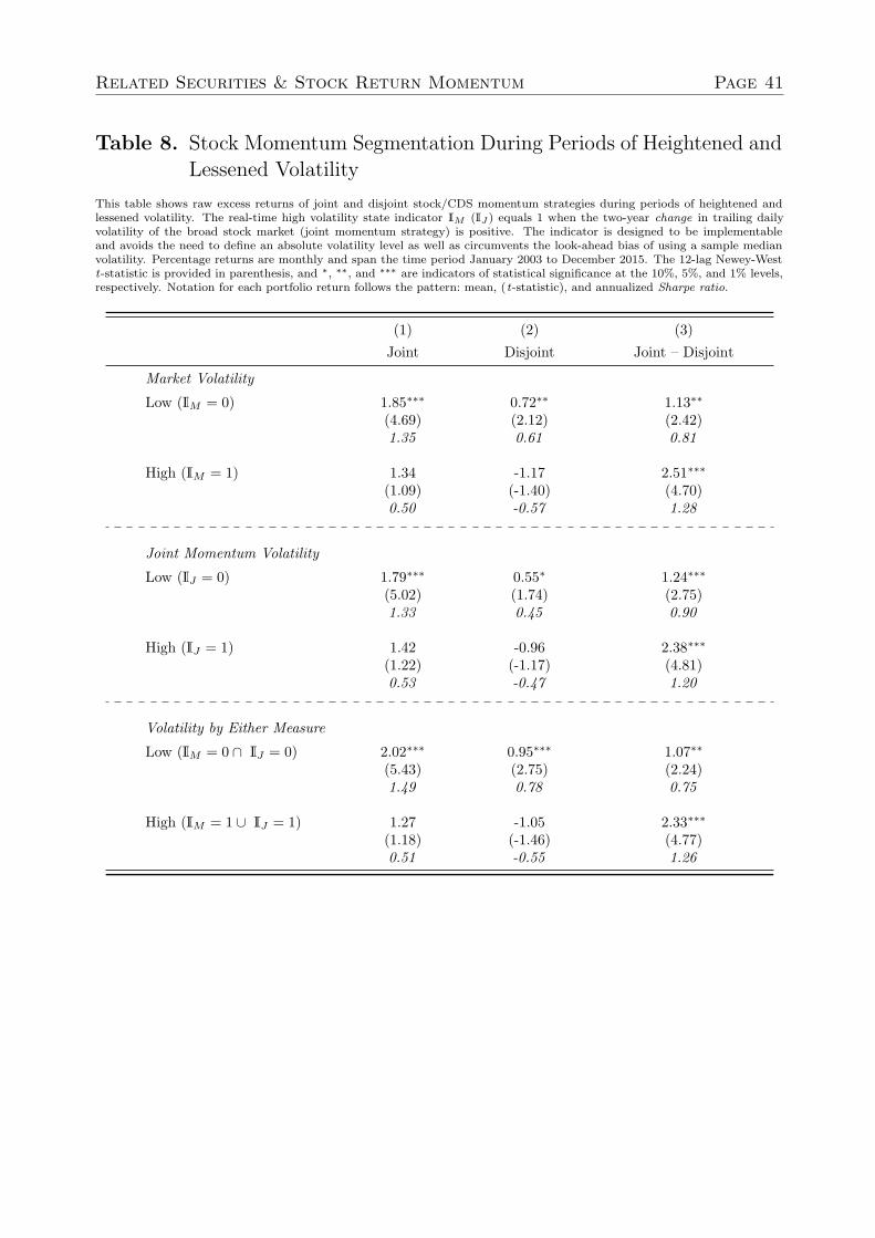
Related Securities & Stock Return Momentum Page 41
Table 8. Stock Momentum Segmentation During Periods of Heightened andLessened Volatility
This table shows raw excess returns of joint and disjoint stock/CDS momentum strategies during periods of heightened andlessened volatility. The real-time high volatility state indicator IM (IJ ) equals 1 when the two-year change in trailing dailyvolatility of the broad stock market (joint momentum strategy) is positive. The indicator is designed to be implementableand avoids the need to define an absolute volatility level as well as circumvents the look-ahead bias of using a sample medianvolatility. Percentage returns are monthly and span the time period January 2003 to December 2015. The 12-lag Newey-Westt-statistic is provided in parenthesis, and ∗, ∗∗, and ∗∗∗ are indicators of statistical significance at the 10%, 5%, and 1% levels,respectively. Notation for each portfolio return follows the pattern: mean, (t-statistic), and annualized Sharpe ratio.
(1) (2) (3)Joint Disjoint Joint – Disjoint
Market Volatility
Low (IM = 0) 1.85∗∗∗ 0.72∗∗ 1.13∗∗(4.69) (2.12) (2.42)1.35 0.61 0.81
High (IM = 1) 1.34 -1.17 2.51∗∗∗(1.09) (-1.40) (4.70)0.50 -0.57 1.28
Joint Momentum Volatility
Low (IJ = 0) 1.79∗∗∗ 0.55∗ 1.24∗∗∗(5.02) (1.74) (2.75)1.33 0.45 0.90
High (IJ = 1) 1.42 -0.96 2.38∗∗∗(1.22) (-1.17) (4.81)0.53 -0.47 1.20
Volatility by Either Measure
Low (IM = 0 ∩ IJ = 0) 2.02∗∗∗ 0.95∗∗∗ 1.07∗∗(5.43) (2.75) (2.24)1.49 0.78 0.75
High (IM = 1 ∪ IJ = 1) 1.27 -1.05 2.33∗∗∗(1.18) (-1.46) (4.77)0.51 -0.55 1.26
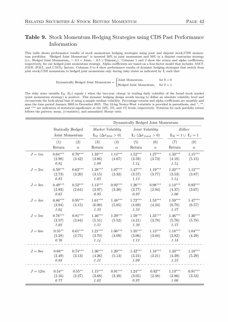
Related Securities & Stock Return Momentum Page 42
Table 9. Stock Momentum Hedging Strategies using CDS Past PerformanceInformation
This table shows performance results of stock momentum hedging strategies using joint and disjoint stock/CDS momen-tum portfolios. “Hedged Joint Momentum” is invested 50% in joint momentum and 50% in a disjoint contrarian strategy(i.e., Hedged Joint Momentumt = 0.5 × Jointt − 0.5 × Disjointt). Columns 1 and 2 show the return and alpha coefficients,respectively, for our hedged joint momentum strategy. Alpha coefficients are based on a four-factor model that includes MKT ,SMB, HML, and UMDS factors. Columns 3 to 8 show performance results of dynamic hedging strategies that switch fromjoint stock/CDS momentum to hedged joint momentum only during risky states as indicated by I, such that
Dynamically Hedged Joint Momentum =
{Joint Momentum, for I = 0
Hedged Joint Momentum, for I = 1.
The risky state variable IM (IJ ) equals 1 when the two-year change in trailing daily volatility of the broad stock market(joint momentum strategy) is positive. This dynamic hedging design avoids having to define an absolute volatility level andcircumvents the look-ahead bias of using a sample median volatility. Percentage returns and alpha coefficients are monthly andspan the time period January 2003 to December 2015. The 12-lag Newey-West t-statistic is provided in parenthesis, and ∗, ∗∗,and ∗∗∗ are indicators of statistical significance at the 10%, 5%, and 1% levels, respectively. Notation for each portfolio returnfollows the pattern: mean, (t-statistic), and annualized Sharpe ratio.
Dynamically Hedged Joint Momentum
Statically Hedged Market Volatility Joint Volatility EitherJoint Momentum IM (∆σMkt > 0) IJ (∆σJoint > 0) IM = 1 ∪ IJ = 1
(1) (2) (3) (4) (5) (6) (7) (8)Return α Return α Return α Return α
J = 1m 0.64∗∗∗ 0.70∗∗∗ 1.33∗∗∗ 1.14∗∗∗ 1.52∗∗∗ 1.27∗∗∗ 1.33∗∗∗ 1.15∗∗∗(2.98) (3.42) (3.86) (4.67) (3.59) (3.73) (4.18) (5.15)0.84 1.08 1.14 1.14
J = 2m 0.59∗∗∗ 0.63∗∗∗ 1.28∗∗∗ 1.07∗∗∗ 1.47∗∗∗ 1.19∗∗∗ 1.32∗∗∗ 1.12∗∗∗(2.73) (3.20) (3.15) (3.32) (3.57) (3.77) (3.53) (3.87)0.85 1.05 1.13 1.14
J = 3m 0.49∗∗∗ 0.52∗∗∗ 1.13∗∗∗ 0.92∗∗∗ 1.26∗∗∗ 0.98∗∗∗ 1.14∗∗∗ 0.93∗∗∗(2.93) (2.64) (3.97) (3.30) (3.77) (2.94) (4.37) (3.67)0.65 0.95 0.97 1.00
J = 4m 0.86∗∗∗ 0.95∗∗∗ 1.61∗∗∗ 1.48∗∗∗ 1.72∗∗∗ 1.53∗∗∗ 1.59∗∗∗ 1.47∗∗∗(3.94) (4.15) (6.00) (5.85) (4.69) (4.24) (6.78) (6.57)1.04 1.32 1.33 1.37
J = 5m 0.76∗∗∗ 0.81∗∗∗ 1.46∗∗∗ 1.29∗∗∗ 1.58∗∗∗ 1.35∗∗∗ 1.46∗∗∗ 1.30∗∗∗(3.57) (3.84) (5.51) (5.52) (4.21) (3.78) (5.76) (5.78)1.02 1.31 1.30 1.37
J = 6m 0.55∗∗ 0.61∗∗∗ 1.21∗∗∗ 1.06∗∗∗ 1.35∗∗∗ 1.13∗∗∗ 1.18∗∗∗ 1.04∗∗∗(2.28) (2.75) (3.70) (4.09) (3.06) (3.04) (3.82) (4.29)0.76 1.14 1.12 1.18
J = 9m 0.68∗∗ 0.74∗∗∗ 1.36∗∗∗ 1.20∗∗∗ 1.42∗∗∗ 1.18∗∗∗ 1.33∗∗∗ 1.18∗∗∗(2.49) (3.13) (4.26) (5.13) (3.24) (3.21) (4.39) (5.29)0.88 1.21 1.09 1.23
J = 12m 0.54∗∗ 0.55∗∗ 1.15∗∗∗ 0.91∗∗∗ 1.24∗∗∗ 0.92∗∗ 1.13∗∗∗ 0.91∗∗∗(2.16) (2.27) (3.68) (3.49) (3.05) (2.48) (3.86) (3.53)0.77 1.02 0.97 1.06
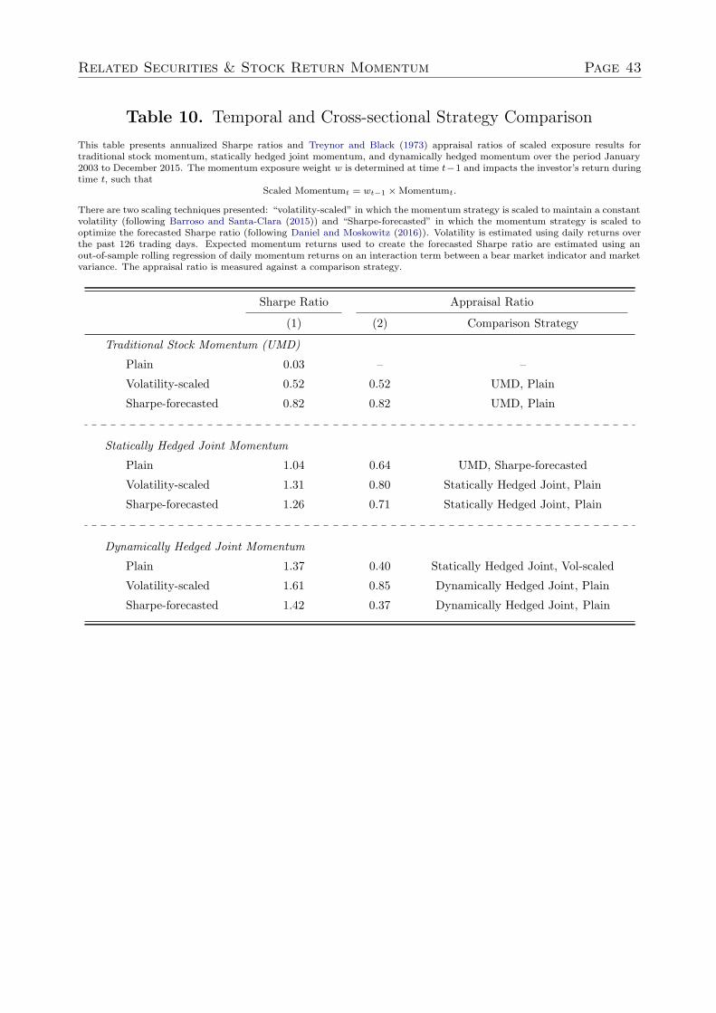
Related Securities & Stock Return Momentum Page 43
Table 10. Temporal and Cross-sectional Strategy Comparison
This table presents annualized Sharpe ratios and Treynor and Black (1973) appraisal ratios of scaled exposure results fortraditional stock momentum, statically hedged joint momentum, and dynamically hedged momentum over the period January2003 to December 2015. The momentum exposure weight w is determined at time t−1 and impacts the investor’s return duringtime t, such that
Scaled Momentumt = wt−1 × Momentumt.
There are two scaling techniques presented: “volatility-scaled” in which the momentum strategy is scaled to maintain a constantvolatility (following Barroso and Santa-Clara (2015)) and “Sharpe-forecasted” in which the momentum strategy is scaled tooptimize the forecasted Sharpe ratio (following Daniel and Moskowitz (2016)). Volatility is estimated using daily returns overthe past 126 trading days. Expected momentum returns used to create the forecasted Sharpe ratio are estimated using anout-of-sample rolling regression of daily momentum returns on an interaction term between a bear market indicator and marketvariance. The appraisal ratio is measured against a comparison strategy.
Sharpe Ratio Appraisal Ratio
(1) (2) Comparison Strategy
Traditional Stock Momentum (UMD)
Plain 0.03 – –
Volatility-scaled 0.52 0.52 UMD, Plain
Sharpe-forecasted 0.82 0.82 UMD, Plain
Statically Hedged Joint Momentum
Plain 1.04 0.64 UMD, Sharpe-forecasted
Volatility-scaled 1.31 0.80 Statically Hedged Joint, Plain
Sharpe-forecasted 1.26 0.71 Statically Hedged Joint, Plain
Dynamically Hedged Joint Momentum
Plain 1.37 0.40 Statically Hedged Joint, Vol-scaled
Volatility-scaled 1.61 0.85 Dynamically Hedged Joint, Plain
Sharpe-forecasted 1.42 0.37 Dynamically Hedged Joint, Plain
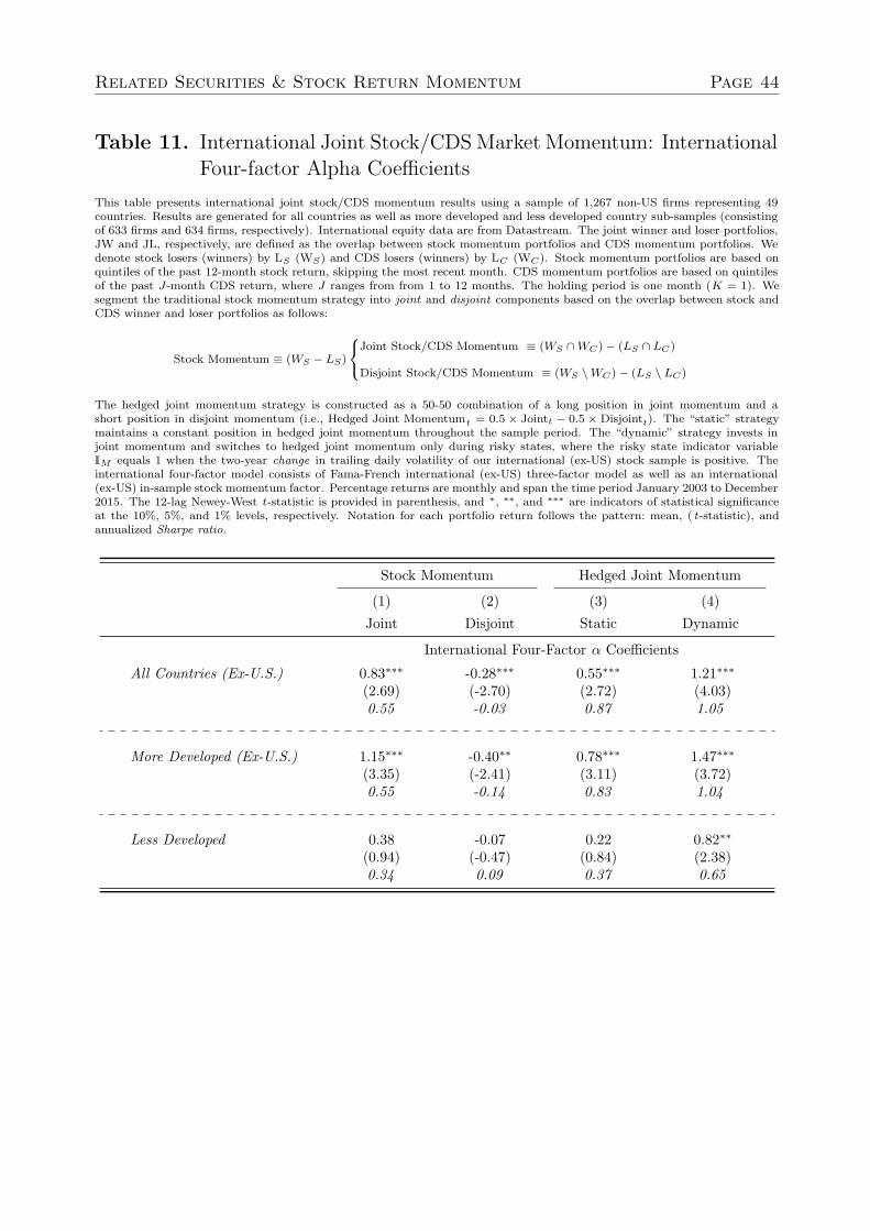
Related Securities & Stock Return Momentum Page 44
Table 11. International Joint Stock/CDS Market Momentum: InternationalFour-factor Alpha Coefficients
This table presents international joint stock/CDS momentum results using a sample of 1,267 non-US firms representing 49countries. Results are generated for all countries as well as more developed and less developed country sub-samples (consistingof 633 firms and 634 firms, respectively). International equity data are from Datastream. The joint winner and loser portfolios,JW and JL, respectively, are defined as the overlap between stock momentum portfolios and CDS momentum portfolios. Wedenote stock losers (winners) by LS (WS) and CDS losers (winners) by LC (WC). Stock momentum portfolios are based onquintiles of the past 12-month stock return, skipping the most recent month. CDS momentum portfolios are based on quintilesof the past J-month CDS return, where J ranges from from 1 to 12 months. The holding period is one month (K = 1). Wesegment the traditional stock momentum strategy into joint and disjoint components based on the overlap between stock andCDS winner and loser portfolios as follows:
Stock Momentum ≡ (WS − LS)
⎧⎨
⎩
Joint Stock/CDS Momentum ≡ (WS ∩ WC) − (LS ∩ LC)
Disjoint Stock/CDS Momentum ≡ (WS \ WC) − (LS \ LC)
The hedged joint momentum strategy is constructed as a 50-50 combination of a long position in joint momentum and ashort position in disjoint momentum (i.e., Hedged Joint Momentumt = 0.5 × Jointt − 0.5 × Disjointt). The “static” strategymaintains a constant position in hedged joint momentum throughout the sample period. The “dynamic” strategy invests injoint momentum and switches to hedged joint momentum only during risky states, where the risky state indicator variableIM equals 1 when the two-year change in trailing daily volatility of our international (ex-US) stock sample is positive. Theinternational four-factor model consists of Fama-French international (ex-US) three-factor model as well as an international(ex-US) in-sample stock momentum factor. Percentage returns are monthly and span the time period January 2003 to December2015. The 12-lag Newey-West t-statistic is provided in parenthesis, and ∗, ∗∗, and ∗∗∗ are indicators of statistical significanceat the 10%, 5%, and 1% levels, respectively. Notation for each portfolio return follows the pattern: mean, ( t-statistic), andannualized Sharpe ratio.
Stock Momentum Hedged Joint Momentum
(1) (2) (3) (4)Joint Disjoint Static Dynamic
International Four-Factor α Coefficients
All Countries (Ex-U.S.) 0.83∗∗∗ -0.28∗∗∗ 0.55∗∗∗ 1.21∗∗∗(2.69) (-2.70) (2.72) (4.03)0.55 -0.03 0.87 1.05
More Developed (Ex-U.S.) 1.15∗∗∗ -0.40∗∗ 0.78∗∗∗ 1.47∗∗∗(3.35) (-2.41) (3.11) (3.72)0.55 -0.14 0.83 1.04
Less Developed 0.38 -0.07 0.22 0.82∗∗(0.94) (-0.47) (0.84) (2.38)0.34 0.09 0.37 0.65
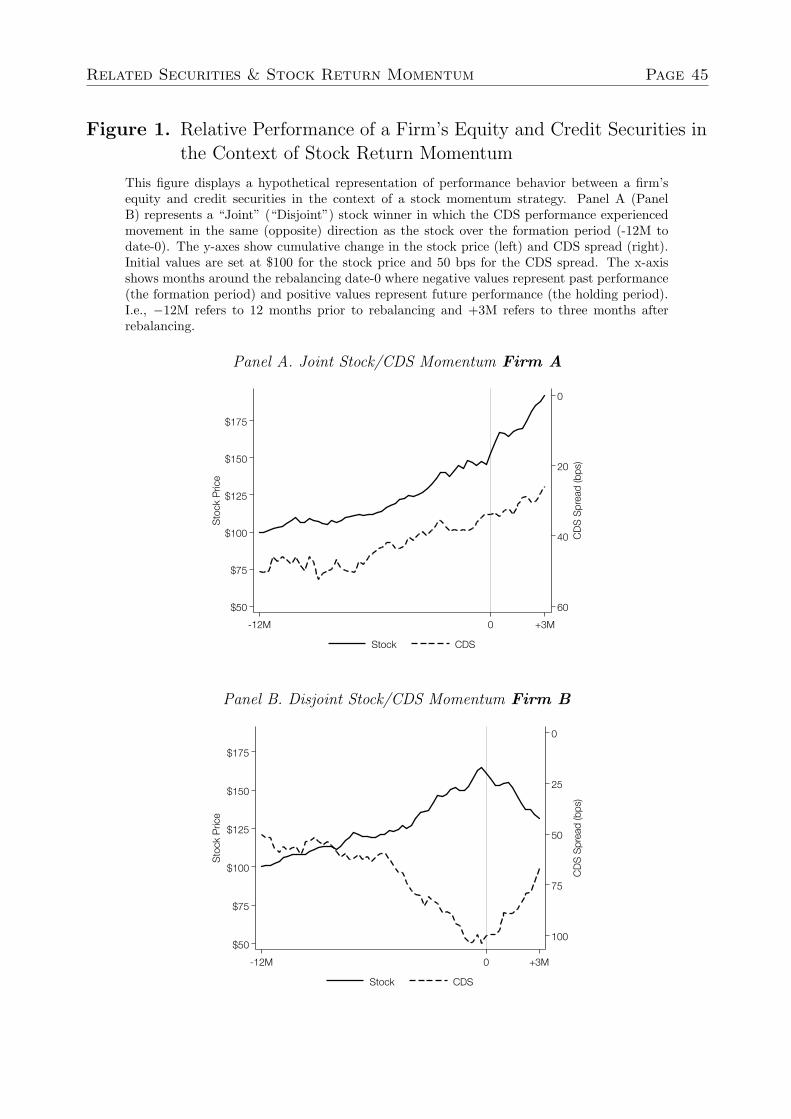
Related Securities & Stock Return Momentum Page 45
Figure 1. Relative Performance of a Firm’s Equity and Credit Securities inthe Context of Stock Return Momentum
This figure displays a hypothetical representation of performance behavior between a firm’sequity and credit securities in the context of a stock momentum strategy. Panel A (PanelB) represents a “Joint” (“Disjoint”) stock winner in which the CDS performance experiencedmovement in the same (opposite) direction as the stock over the formation period (-12M todate-0). The y-axes show cumulative change in the stock price (left) and CDS spread (right).Initial values are set at $100 for the stock price and 50 bps for the CDS spread. The x-axisshows months around the rebalancing date-0 where negative values represent past performance(the formation period) and positive values represent future performance (the holding period).I.e., −12M refers to 12 months prior to rebalancing and +3M refers to three months afterrebalancing.
Panel A. Joint Stock/CDS Momentum Firm A
0
20
40
60
CD
S S
pre
ad
(b
ps)
$50
$75
$100
$125
$150
$175
Sto
ck
Pric
e
-12M +3M0
Stock CDS
Panel B. Disjoint Stock/CDS Momentum Firm B
0
25
50
75
100
CD
S S
pre
ad
(b
ps)
$50
$100
$75
$125
$150
$175
Sto
ck
Pric
e
-12M +3M0
Stock CDS
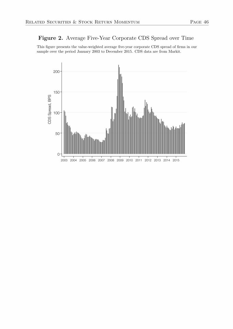
Related Securities & Stock Return Momentum Page 46
Figure 2. Average Five-Year Corporate CDS Spread over Time
This figure presents the value-weighted average five-year corporate CDS spread of firms in oursample over the period January 2003 to December 2015. CDS data are from Markit.
0
50
100
150
200
CDS
Spre
ad, B
PS
2003 2004 2005 2006 2007 2008 2009 2010 2011 2012 2013 2014 2015
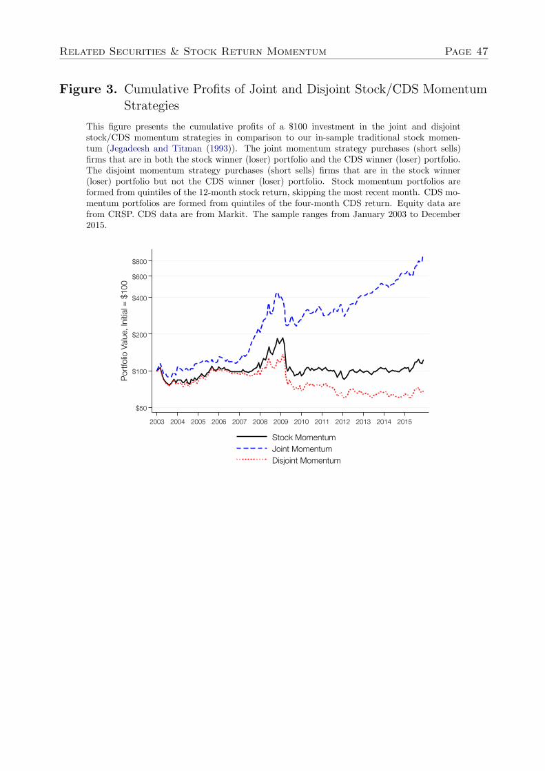
Related Securities & Stock Return Momentum Page 47
Figure 3. Cumulative Profits of Joint and Disjoint Stock/CDS MomentumStrategies
This figure presents the cumulative profits of a $100 investment in the joint and disjointstock/CDS momentum strategies in comparison to our in-sample traditional stock momen-tum (Jegadeesh and Titman (1993)). The joint momentum strategy purchases (short sells)firms that are in both the stock winner (loser) portfolio and the CDS winner (loser) portfolio.The disjoint momentum strategy purchases (short sells) firms that are in the stock winner(loser) portfolio but not the CDS winner (loser) portfolio. Stock momentum portfolios areformed from quintiles of the 12-month stock return, skipping the most recent month. CDS mo-mentum portfolios are formed from quintiles of the four-month CDS return. Equity data arefrom CRSP. CDS data are from Markit. The sample ranges from January 2003 to December2015.
$50
$100
$200
$400
$600
$800
Port
folio
Valu
e, In
itial =
$100
2003 2004 2005 2006 2007 2008 2009 2010 2011 2012 2013 2014 2015
Stock Momentum
Joint Momentum
Disjoint Momentum
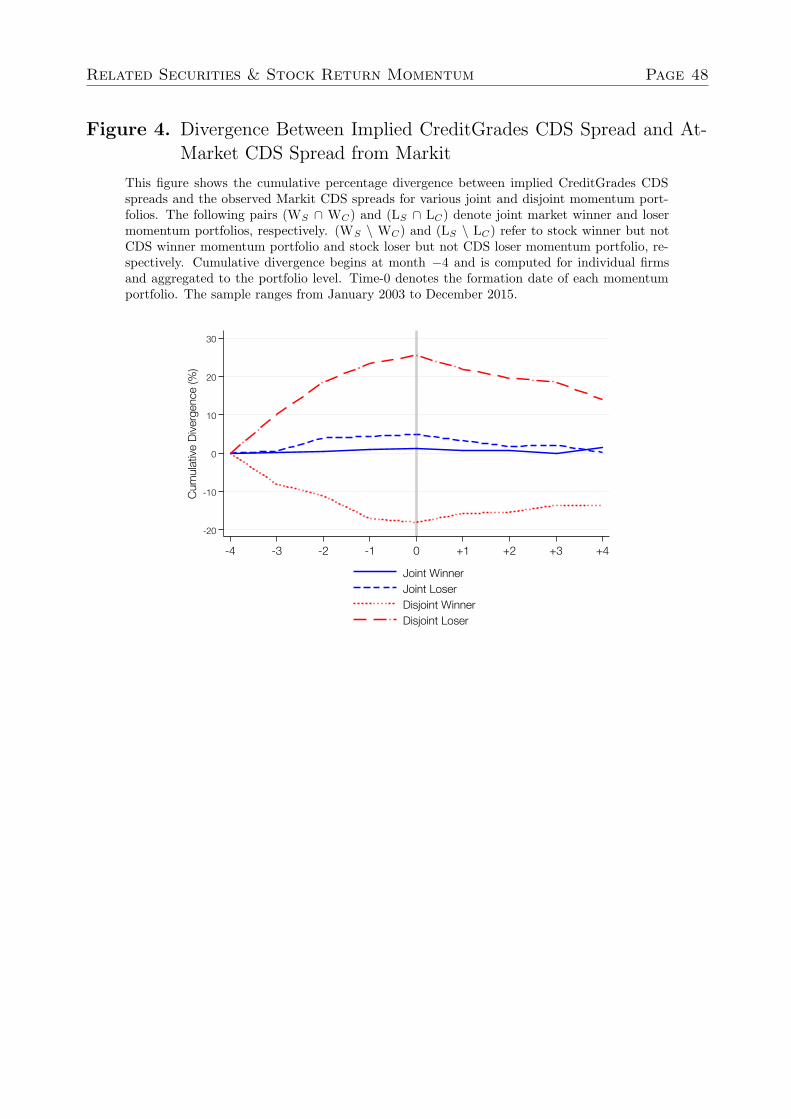
Related Securities & Stock Return Momentum Page 48
Figure 4. Divergence Between Implied CreditGrades CDS Spread and At-Market CDS Spread from Markit
This figure shows the cumulative percentage divergence between implied CreditGrades CDSspreads and the observed Markit CDS spreads for various joint and disjoint momentum port-folios. The following pairs (WS ∩ WC) and (LS ∩ LC) denote joint market winner and losermomentum portfolios, respectively. (WS \ WC) and (LS \ LC) refer to stock winner but notCDS winner momentum portfolio and stock loser but not CDS loser momentum portfolio, re-spectively. Cumulative divergence begins at month −4 and is computed for individual firmsand aggregated to the portfolio level. Time-0 denotes the formation date of each momentumportfolio. The sample ranges from January 2003 to December 2015.
-20
-10
0
10
20
30
Cum
ula
tive D
iverg
ence (%
)
-4 -3 -2 -1 0 +1 +2 +3 +4 +5 +6
Joint Winner
Joint Loser
Disjoint Winner
Disjoint Loser
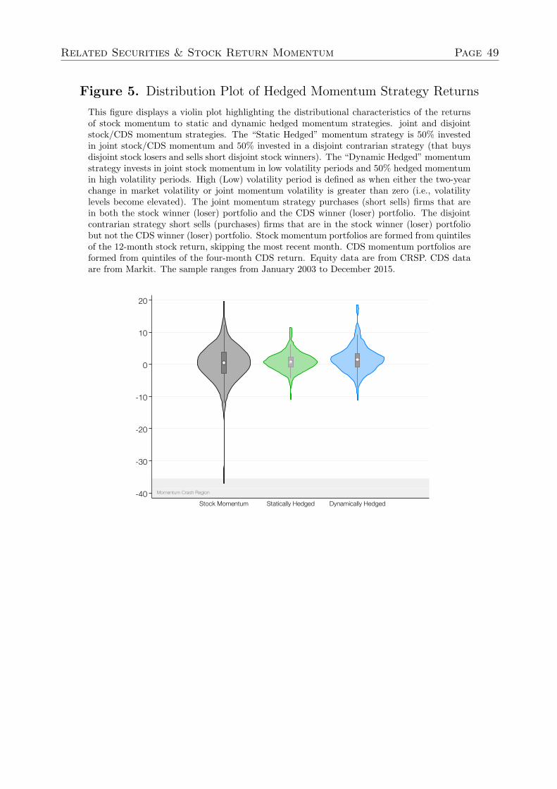
Related Securities & Stock Return Momentum Page 49
Figure 5. Distribution Plot of Hedged Momentum Strategy Returns
This figure displays a violin plot highlighting the distributional characteristics of the returnsof stock momentum to static and dynamic hedged momentum strategies. joint and disjointstock/CDS momentum strategies. The “Static Hedged” momentum strategy is 50% investedin joint stock/CDS momentum and 50% invested in a disjoint contrarian strategy (that buysdisjoint stock losers and sells short disjoint stock winners). The “Dynamic Hedged” momentumstrategy invests in joint stock momentum in low volatility periods and 50% hedged momentumin high volatility periods. High (Low) volatility period is defined as when either the two-yearchange in market volatility or joint momentum volatility is greater than zero (i.e., volatilitylevels become elevated). The joint momentum strategy purchases (short sells) firms that arein both the stock winner (loser) portfolio and the CDS winner (loser) portfolio. The disjointcontrarian strategy short sells (purchases) firms that are in the stock winner (loser) portfoliobut not the CDS winner (loser) portfolio. Stock momentum portfolios are formed from quintilesof the 12-month stock return, skipping the most recent month. CDS momentum portfolios areformed from quintiles of the four-month CDS return. Equity data are from CRSP. CDS dataare from Markit. The sample ranges from January 2003 to December 2015.
Momentum Crash Region-40
-30
-20
-10
0
10
20
Stock Momentum Statically Hedged Dynamically Hedged
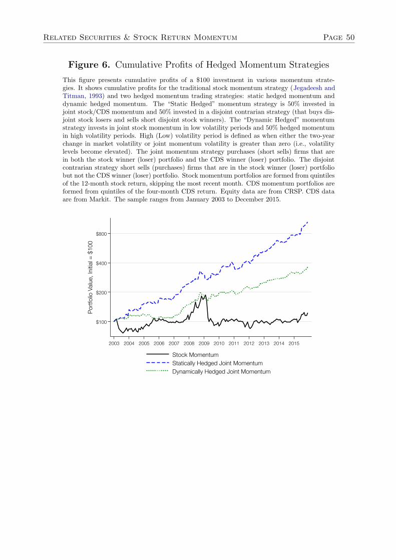
Related Securities & Stock Return Momentum Page 50
Figure 6. Cumulative Profits of Hedged Momentum Strategies
This figure presents cumulative profits of a $100 investment in various momentum strate-gies. It shows cumulative profits for the traditional stock momentum strategy (Jegadeesh andTitman, 1993) and two hedged momentum trading strategies: static hedged momentum anddynamic hedged momentum. The “Static Hedged” momentum strategy is 50% invested injoint stock/CDS momentum and 50% invested in a disjoint contrarian strategy (that buys dis-joint stock losers and sells short disjoint stock winners). The “Dynamic Hedged” momentumstrategy invests in joint stock momentum in low volatility periods and 50% hedged momentumin high volatility periods. High (Low) volatility period is defined as when either the two-yearchange in market volatility or joint momentum volatility is greater than zero (i.e., volatilitylevels become elevated). The joint momentum strategy purchases (short sells) firms that arein both the stock winner (loser) portfolio and the CDS winner (loser) portfolio. The disjointcontrarian strategy short sells (purchases) firms that are in the stock winner (loser) portfoliobut not the CDS winner (loser) portfolio. Stock momentum portfolios are formed from quintilesof the 12-month stock return, skipping the most recent month. CDS momentum portfolios areformed from quintiles of the four-month CDS return. Equity data are from CRSP. CDS dataare from Markit. The sample ranges from January 2003 to December 2015.
$100
$200
$400
$800
Por
tfolio
Val
ue, I
nitia
l = $
100
2003 2004 2005 2006 2007 2008 2009 2010 2011 2012 2013 2014 2015
Stock MomentumStatically Hedged Joint MomentumDynamically Hedged Joint Momentum

Related Securities & Stock Return Momentum Page 51
Figure 7. Global Hedged Momentum (50% U.S., 50% Non-U.S.)
This figure presents cumulative profits of a $100 investment in global traditional stock momen-tum and our dynamic hedge momentum strategies. Each global portfolio maintains 50% in theU.S.-based strategy and 50% in non-U.S.-based strategy. Our “Dynamic Hedged Momentum”strategy invests in joint momentum during low volatility periods and hedged joint momen-tum (50% in joint momentum and 50% in disjoint contrarian) during high volatility periods.The joint momentum strategy purchases (short sells) firms that are in both the stock winner(loser) portfolio and the CDS winner (loser) portfolio. The disjoint contrarian strategy shortsells (purchases) firms that are in the stock winner (loser) portfolio but not the CDS winner(loser) portfolio. Stock momentum portfolios are formed from quintiles of the 12-month stockreturn, skipping the most recent month. CDS momentum portfolios are formed from quintilesof the four-month CDS return. U.S. equity data are from CRSP and international equity dataare from Datastream. CDS data are from Markit. The sample ranges from January 2003 toDecember 2015.
$100
$200
$400
$800
Por
tfolio
Val
ue, I
nitia
l = $
100
2003 2004 2005 2006 2007 2008 2009 2010 2011 2012 2013 2014 2015
Global Stock MomentumGlobal Dynamically Hedged Joint Momentum

Related Securities & Stock Return Momentum Page 52
Appendices
A Variable Definitions
Variable Name Description Source
Market CapitalizationEquity market capitalization, defined as the number of commonshares outstanding multiplied by the price of the firm’s stock atthe time of portfolio formation. (USD, $ Billions)
CRSP
Stock Return (%)The holding period percentage return of the firm’s stock over thecourse of the month.
CRSP
CDS Spread (bps)
Credit default swap (CDS) spreads (reported in basis points) arebased on daily quoted spreads collected from a number ofmarket makers. Each composite spread consists of at least twocontributors and has passed a rigorous cleaning test to ensureaccuracy and reliability.
Markit Group
CDS Return (%)
The holding period percentage return of the firm’s CDS to theprotection seller over the course of the month. Computed as themarked-to-market dollar change in value of CDS contractdivided by notional value.
Markit Group
CDS DepthThe number of good contributions used to construct thecomposite spread. Markit requires at least two.
Markit Group
S&P Credit RatingStandard and Poor’s credit rating for the company (provided atthe end of each month). It is converted to a numerical score inwhich 1=AAA, 2=AA+, 3=AA, . . .
Standard & Poors:Compustat NorthAmerica, MonthlyUpdates

Related Securities & Stock Return Momentum Page 53
B Factor Definitions
FactorName
Description Source
MKT The value-weighted excess return on all NYSE, AMEX, and Nasdaq stocks. Ken French’s Website
SMBThe value-weighted return on a portfolio of small stocks minus a portfolio of bigstocks.
Ken French’s Website
HMLThe value-weighted return on a portfolio of stocks with high book-to-marketequity ratios minus a portfolio of stocks with low book-to-market equity ratios.
Ken French’s Website
UMDThe value-weighted return on a portfolio of stocks with relative goodperformance over the last 12 months minus a portfolio of stocks with relativebad performance over the last 12 months.
Ken French’s Website
UMDS
Traditional stock momentum strategy using firms in our sample. Stocks aresorted based on past 12-month return, skipping the most recent month, andassigned to quintiles. The long/short strategy is formed by purchasing stocks inthe highest quintile and selling short stocks in the lowest quintile, andrebalanced monthly. Returns are value-weighted.
CRSP
LIQThe value-weighted return on a portfolio of stocks with high liquidity betaminus a portfolio of stocks with low liquidity beta.
Lubos Pastor’s Website
SUE
Stocks are sorted based on the standardized unexpected earnings (SUE), andassigned to quintiles. SUE is defined as the most recent EPS minus EPS twelvemonths ago, divided by the standard deviation of quarterly EPS over the lasteight quarters. The long/short strategy is formed by purchasing stocks in thehighest quintile and selling short stocks in the lowest quintile, rebalancedmonthly. Returns are value-weighted.
CRSP, Compustat
CAR3
Stocks are sorted based on the cumulative abnormal three-day return (CAR3),and assigned to quintiles. CAR3 is defined as cumulative three-day returnaround the most recent earnings announcement minus the market returnmultiplied by beta. The long/short strategy is formed by purchasing stocks inthe highest quintile and selling short stocks in the lowest quintile, rebalancedmonthly. Returns are value-weighted.
CRSP, Compustat

Related Securities & Stock Return Momentum Page 54
C CDS Return Computation
First, we provide a standard CDS pricing model as in O’Kane (2008).30 Then, through this
pricing framework, we define the mark-to-market value of a CDS with a unit $1-notional
using at-market spread quotes from Markit. The change of these mark-to-market values
over a given holding period determines the CDS holding period return.
C.1 CDS Return: Pricing Framework and Mark-to-market
We split the pricing of a CDS contract with a unit $1-notional into two legs, the premium leg
and protection leg. To simplify our illustration, we assume that we are on the inception date
of a five-year CDS. This fresh five-year contract matures on the first IMM date five years after
the trade date. Since 2003, at any moment in time, the most liquid T−year CDS contract
is the one that matures on the first IMM date T years after the trade date. For example,
a five-year CDS contract trading on 12/20/2013 matures on 3/20/2018. The premium leg
has two components. First, there are 21 scheduled premium payments on a quarterly cycle
with the CDS IMM dates – the 20th of March, June, September, and December – until the
maturity date as long as the reference entity survives. When there is a credit event, there is
a payment of the premium that has accrued since the last quarterly premium payment date.
This is the second component of the premium leg.
Let us denote the quarterly premium payment dates over a five-year horizon by ti, i =
1, 2, . . . , 21, and let t0 denote our valuation date. Given the quoted spread of S0 at time-t0,
the present value of the first component of the premium leg becomes
S0
n=21∑
n=1
∆(tn−1, tn)Q(t0, tn)Z(t0, tn), (3)
where ∆(tn−1, tn) denotes the accrual factor for the time period, [tn−1, tn], and Q(t0, tn) and
Z(t0, tn), respectively, denote the survival probability of the reference entity and default-free
discounting factor for the time period, [t0, tn].
Now, we consider the premium accrued at default for the nth premium period, [tn−1, tn].
30Under the flat hazard rate assumption, O’Kane’s (2008) pricing model becomes an ISDA CDS Standardmodel used by Markit.

Related Securities & Stock Return Momentum Page 55
Over an infinitesimal time interval, [s, s + ds] for s ∈ [tn−1, tn], the expected present value of
the premium accrued upon default is given by
S0∆(tn−1, s) (−dQ(t0, s)) Z(t0, s). (4)
Then, the value of the premium accrued upon default for all 21 premium periods is given
by
S0
n=21∑
n=1
∫ tn
tn−1
∆(tn−1, s)Z(t0, s) (−dQ(t0, s)) . (5)
By summing up Eq. (3) and (5), the present value of the premium leg becomes
Premium Leg PV = S0 · RPV 01(t0, t21), (6)
where RPV 01(t0, t21) is given by
RPV 01(t0, t21) =n=21∑
n=1
∆(tn−1, tn)Q(t0, tn)Z(t0, tn)+n=21∑
n=1
∫ tn
tn−1
∆(tn−1, s)Z(t0, s) (−dQ(t0, s)) .
(7)
The integration in the second term in Eq. (7) can be approximated as
∫ tn
tn−1
∆(tn−1, s)Z(t0, s) (−dQ(t0, s)) ≃1
2∆(tn−1, tn)Z(t0, tn) (Q(t0, tn−1) − Q(t0, tn)) . (8)
Thus, we have
RPV 01(t0, t21) =∑n=21
n=1 ∆(tn−1, tn)Z(t0, tn)Q(t0, tn)
+∑n=21
n=112∆(tn−1, tn)Z(t0, tn) (Q(t0, tn−1) − Q(t0, tn)) .
(9)
Assuming a constant loss given default, (1 −R), together with the standard assumption
of independence of interest rate and the default time, we can write the present value of the
protection leg as
Protection Leg PV = (1 − R)∫ t21
t0Z(t0, s) (−dQ(t0, s))
≃ (1 − R)∑n=21
n=1 Z(t0, tn) (Q(t0, tn−1) − Q(t0, tn)) .(10)

Related Securities & Stock Return Momentum Page 56
The second line shows that the integration in the first line is performed by discretizing the
five-year horizon by 21 intervals with each coupon payment date. Here we directly use the
lower bound of the discretized integration.
Combining the present values of the premium and the protection legs gives the mark-
to-market value of a five-year short protection position of a CDS with a unit $1-notional as
V (t0) = S0 · RPV 01(t0, t21) − (1 − R)n=21∑
n=1
Z(t0, tn) (Q(t0, tn−1) − Q(t0, tn)) , (11)
where RPV 01(t0, t21) is as in Eq. (9). For a protection buyer, the mark-to-market value
would be just the opposite, −V (t0).
With the quoted spread, S0, V (t0) = 0 as required.31 However, soon after the inception
of trading, this requirement is no longer true since the market spread of the CDS reference
entity moves from the spread that the protection seller/buyer are locked into.
Finally, with this pricing framework, we can easily define the P&L of a CDS with a unit
$1-notional over a holding period, [t0, t′]. For simplicity, we assume for a moment that this
interval is short enough so that we can ignore any coupon flows and also potential credit
event during this holding period. If we entered as a seller of a protection at time- t0 and
unwind the position at time-t′ by buying a protection on the same reference entity and the
same maturity date, then the CDS holding period excess return is given as
CDS return(t0, t′) = − (S(t′) − S(t0)) · RPV 01(t′, t21). (12)
S(t0) · RPV 01(t′, t21) in the above Eq. (12) denotes the time-t′ value of the protection
we sold at time-t0, and −S(t′) · RPV 01(t′, t21) the time-t′ cost to purchase the protection
on the same reference entity with the same maturity date. If there is a credit event over
our holding period, then the realized return will be equal to −(1 − R̃) where R̃ is a realized
recovery rate upon the credit event. Eq. (12) does not take into account coupon flows during
our holding period and the accrued premium that should be exchanged at each selling and
buying transaction of the default protection. We carefully incorporate these factors when
31If our valuation falls between two consecutive coupon payment dates, the quoted spread will make theclean mark-to-market value zero. We need to adjust for accrued premium since the last coupon paymentdate when we compute the clean mark-to-market.

Related Securities & Stock Return Momentum Page 57
we implement this CDS return framework using the quoted spreads from Markit. The
U.S. $Libor curve retrieved from DataStream is calibrated to fit the Nelson-Siegel-Svensson
(NSS) curve (Nelson and Siegel, 1987; Svensson, 1994), and we construct the default-free
discounting factors using the fitted values of the NSS curve. After all these considerations,
we compute CDS returns based on “clean” P&L’s.
C.2 Implementation of the CDS Returns using Markit Data
As illustrated above, we approach CDS returns from the perspective of the protection seller
(i.e., a negative return corresponds to an increase in credit risk). We compound monthly
trading return of five-year contracts from their daily returns. To compute the CDS return, we
need to construct the survival probability curve on a given valuation date- t′, Q(t′, ti), for i =
1, 2, ..., 21. Instead of bootstrapping this survival probability curve using the quoted spreads
of CDS contracts across entire maturity groups, we assume a flat hazard rate, h(t′, ti) ≡
− 1Q(t′,ti)
∂Q(t′,ti)∂ti
= h for ∀i = 1, 2, . . . , 21, and calibrate the hazard from the quoted spread of
a five-year CDS contract.
It is possible that credit events occur during our monthly holding period. If a credit event
occurs, we need to assign the realized loss given default to the CDS return for that holding
period. We use the realized recovery rate information that we compiled from the Creditex
Group and make appropriate adjustments in our holding period excess returns.
An accrued premium should be adjusted when the CDS trade occurs in between the
quarterly coupon payment interval. There are two different ways the accrued premium
payment is handled during our sample period. Before the 2009 “Big Bang” protocol, the
first premium accrued since the trade date was paid either on the next immediate coupon
date (i.e., short-stub) or the following coupon date (i.e., long-stub), depending on the trade
date. If the trade date fell within a 30-day window prior to the first upcoming coupon date,
it would follow the long-stub rule and the short-stub otherwise. However, post-“Big Bang,”
these complicated accrued premium payment rules disappeared, and now the single-name
CDS contracts trade just like the Markit CDS indices where the new protection seller will
receive the full quarterly coupon on each coupon payment date. Any “over”-paid premium to
this seller by the protection buyer is rebated upfront. We follow this post-“Big Bang” coupon
convention when we adjust the accrued premium to get the clean P&L of our CDS trading.

Related Securities & Stock Return Momentum Page 58
We compute the P&L’s on the running spread basis, instead of using fixed 100 bps/500 bps
coupons with upfront adjustments. Since the default-free rate during our sample period is
relatively low, the potential errors in our treatment of the stub algorithms should be minimal
for CDS returns in the pre-“Big Bang” period.
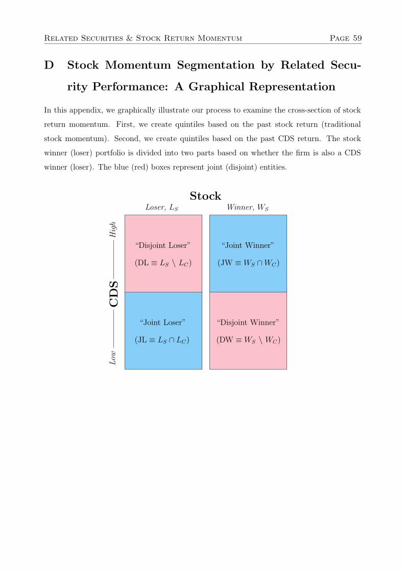
Related Securities & Stock Return Momentum Page 59
D Stock Momentum Segmentation by Related Secu-
rity Performance: A Graphical Representation
In this appendix, we graphically illustrate our process to examine the cross-section of stock
return momentum. First, we create quintiles based on the past stock return (traditional
stock momentum). Second, we create quintiles based on the past CDS return. The stock
winner (loser) portfolio is divided into two parts based on whether the firm is also a CDS
winner (loser). The blue (red) boxes represent joint (disjoint) entities.
CD
SH
igh
Low
StockLoser, LS Winner, WS
(DL ≡ LS \ LC)
“Disjoint Loser”
(JW ≡ WS ∩ WC)
“Joint Winner”
(DW ≡ WS \ WC)
“Disjoint Winner”
(JL ≡ LS ∩ LC)
“Joint Loser”

Related Securities & Stock Return Momentum Page 60
E CreditGrades Hedge Ratio
We use the CreditGrades hedge ratio to implement the capital structure arbitrage described
in Section 3.4 of our main text. The hedge ratio is estimated on each rebalancing date.
We scale our CDS position using these hedge ratios during the capital structure arbitrage
trade. The CreditGrades model, which is based on Black and Cox (1976) and Leland (1994),
is known to be commonly used by practitioners in the implementation of capital structure
arbitrage.
Similar to Merton (1974), the CreditGrades model assumes that firm value V follows
a standard Brown motion (W ) with volatility σV . The firm’s debt-per-share D remains
constant, and the recovery rate L follows a lognormal distribution with mean L̄. The model
allows the potential for default to occur before maturity as firm value falls below a specified
threshold (the value of assets that could be recovered in the event of default). The default
threshold is represented as
LD = L̄DeλZ−λ2/2, (13)
where λ2 =Var log(L) and Z is a standard normal variable. Thus, starting with initial firm
value V0, default does not occur as long as
V0eσV Wt−σ2
V t/2 > L̄DeλZ−λ2/2. (14)
We derive the T -year CreditGrades-implied CDS spread c using the firm’s stock price S,
debt-per-share D (total liabilities divided by common shares outstanding), standard devia-
tion of the global recovery rate λ (assumed to be 0.3), bond-specific recovery rate R (assumed
to be 0.5), equity volatility σS (the annualized standard deviation of weekly returns over the
past year), the risk-free rate r (1-year Treasury rate), CDS contract maturity T (set to be
5), and the mean global recovery rate L̄. Similar to Yu (2006), we calibrate L̄ for each firm
by minimizing the sum of squared differences between the CreditGrades model spread and
observed Markit spread using the first 10 days of available data. This allows each firm to
have a constant L̄ that reflects a recovery expectation implied by the data. The implied

Related Securities & Stock Return Momentum Page 61
T -year CDS spread is
cT = r(1 − R)1 − q(0) + H(T )
q(0) − q(T )e−rT − H(T ), (15)
where survival probability q(T ) is expressed as
q(T ) = Φ
[−
√σ2
T T + λ2
2+
ln d√σ2
T T + λ2
]− dΦ
[−
√σ2
T T + λ2
2− ln d√
σ2T T + λ2
], (16)
with Φ(·) being the cumulative normal distribution function, and
H(T ) = erξ [G(T + ξ) − G(ξ)] , (17)
G(T ) = dz+0.5 · Φ[− ln d
σV
√T
− zσV
√T
]+ dz+0.5 · Φ
[− ln d
σV
√T
+ zσV
√T
], (18)
d =V0
L̄Deλ2
, (19)
ξ =λ2
σ2V
, (20)
and
z =
√1
4+
2r
σ2V
. (21)
To relate the asset volatility to equity volatility, CreditGrades uses a simple approximation
for the asset value of V = S + L̄D, which gives σV = σSS/(S + L̄D).
At the time a CDS contract is written, the spread is set such that the credit protection
buyer and seller positions are equivalent, resulting in the value of the contract π being zero.
The spread will change over time as the equity value changes, and the value of the contract
will change proportional to the spread. The hedge ratio δ between the stock S and a T -year
CDS contract πT is expressed as
δ =∂πT
∂S=
1
r
∂cT
∂S
(q(0) − q(T )e−Tr − erξ [G(T + ξ) − G(T )]
)(22)

Related Securities & Stock Return Momentum Page 62
where ∂cT∂S is numerically computed.
Internet Appendix: Related Securities and
the Cross-section of Stock Return Momentum
Jongsub Lee∗, Andy Naranjo†, and Stace Sirmans‡
∗University of Florida, Assistant Professor, Tel: 352.273.4966, Email: [email protected]†University of Florida, Emerson-Merrill Lynch Professor of Finance and Chairman of Finance Department,
Tel: 352.392.3781, Email: [email protected]‡University of Arkansas, Assistant Professor, Tel: 850.459.2039, Email: [email protected]

Internet Appendix Page 1
Contents
A Stock/CDS Momentum Portfolio Statistics 2
B Joint and Disjoint Momentum Profitability at Longer Holding Periods:
Four-Factor Alpha Coefficients 3
C Comparison of Strategies Based on Earnings Momentum (SUE), past CDS
Performance, and past Stock Performance 4
D Marginal Information in past CDS Returns using Various Formation Hori-
zons: Four-Factor Alpha Coefficients 6
E Multi-Term Stock Momentum Strategies: Four-Factor Alpha Coefficients 8
F Factor Exposures of Joint Momentum and Statically Hedged Joint Mo-
mentum 10

Internet Appendix Page 2
A Stock/CDS Momentum Portfolio Statistics
This appendix table provides various statistics of the joint and disjoint stock/CDS momen-
tum portfolios. Number of Unique Entities refers to the total number of unique entities that
appear in the portfolio during the course of the sample period. Each additional statistic
is averaged across all entities in the portfolio during the month and then averaged over all
months in the entire sample period. Size refers to average equity market capitalization de-
fined as end-of-month price multiplied by shares outstanding. S&P Rating is the average
S&P credit rating. Portfolio Turnover measures the average monthly trading activity during
end-of-month rebalancing. The joint momentum strategy is formed by purchasing (short
selling) firms that fall in both the traditional stock winner (loser) portfolio and the CDS
winner (loser) portfolio. The disjoint momentum strategy is formed by purchasing (short
selling) firms that fall in the traditional stock winner (loser) and the CDS loser (winner)
portfolio. The traditional stock momentum strategy is formed by buying winners and selling
losers of quintiles based on the past 12-month stock return, skipping the most recent month.
The CDS momentum portfolios are quintiles of the past four-month CDS return. The sample
period spans January 2003 to December 2015.
Stock Stock Joint Joint Disjoint DisjointWinner Loser Winner Loser Winner Loser
(W) (L) (JW) (JL) (DW) (DL)
No. of Unique Entities 735 695 563 588 713 679
Size ($, billions) $19.1 $15.4 $11.9 $9.7 $22.0 $18.6
S&P Rating BBB- BBB- BB+ BB+ BBB BBB-
Portfolio Turnover 31% 33% 56% 55% 39% 45%

Internet Appendix Page 3
B Joint and Disjoint Momentum Profitability at Longer
Holding Periods: Four-Factor Alpha Coefficients
This table shows the monthly alpha coefficients of joint and disjoint stock/CDS momentum
at longer holding periods. The four-factor model includes the MKT , SMB, HML, and
UMDS factors. Returns longer than one month are constructed so as to avoid an overlapping
returns problem. For example, to calculate the three-month holding period return, we take
the average of the one-month returns of strategies based on the current quintiles, the one-
month lagged quintiles, and the two-month lagged quintiles. Joint stock/CDS momentum
purchases (sells short) stocks in both the top (bottom) past 12-month stock return quintile
and the top (bottom) past four-month CDS return quintile. Disjoint stock/CDS momentum
purchases (sells short) stocks in the top (bottom) past 12-month stock return quintile but not
in the top (bottom) past four-month CDS return quintile. The time period spans January
2003 to December 2015. The 12-lag Newey-West t-statistic is provided in parenthesis, and ∗,
∗∗, and ∗∗∗ are indicators of statistical significance at the 10%, 5%, and 1% levels, respectively.
Notation for each portfolio return follows the pattern: mean, (t-stat), and annualized Sharpe
ratio.
Holding Period (K)
(1) (2) (3) (4) (5) (6)1m 2m 3m 4m 5m 6m
Monthly Four-Factor α Coefficients
Joint Stock/CDS Momentum 1.45∗∗∗ 1.34∗∗∗ 0.95∗∗∗ 0.75∗∗∗ 0.57∗∗∗ 0.56∗∗∗(4.24) (4.36) (3.41) (3.19) (2.64) (2.70)0.81 0.77 0.62 0.58 0.51 0.52
Disoint Stock/CDS Momentum -0.45∗∗∗ -0.45∗∗∗ -0.38∗∗ -0.26∗ -0.17 -0.15(-3.10) (-3.54) (-2.60) (-1.75) (-1.07) (-0.89)-0.05 -0.05 -0.02 0.05 0.10 0.10
Joint – Disjoint 1.90∗∗∗ 1.79∗∗∗ 1.33∗∗∗ 1.02∗∗∗ 0.74∗∗ 0.71∗∗(4.15) (4.45) (3.69) (3.32) (2.55) (2.46)1.04 1.05 0.86 0.77 0.64 0.67

Internet Appendix Page 4
C Comparison of Strategies Based on Earnings Mo-
mentum (SUE), past CDS Performance, and past
Stock Performance
This table shows the results of spanning tests examining various SUE-based strategies as well
as joint stock/CDS momentum. There are three SUE-based strategies in the table. “SUE”
refers to a strategy that purchases (sells short) stocks in the top (bottom) SUE quintile.
“SUE | r2,12” refers to a strategy that purchases (sells short) stocks in the top (bottom) SUE
quintile that is conditioned on the past 12-month stock return. “rS,12 ∩ SUE” refers to a
strategy that purchases (sells short) stocks in both the top (bottom) SUE quintile and the
top (bottom) past 12-month stock return quintile. The firm-level standardized unexpected
earnings (SUE) is computed as the one-year change in quarterly reported earnings divided
by the standard deviation of quarterly earnings changes over the past eight quarters. The
time period spans January 2003 to December 2015. The 12-lag Newey-West t-statistic is
provided in parenthesis, and ∗, ∗∗, and ∗∗∗ are indicators of statistical significance at the 10%,
5%, and 1% levels, respectively.
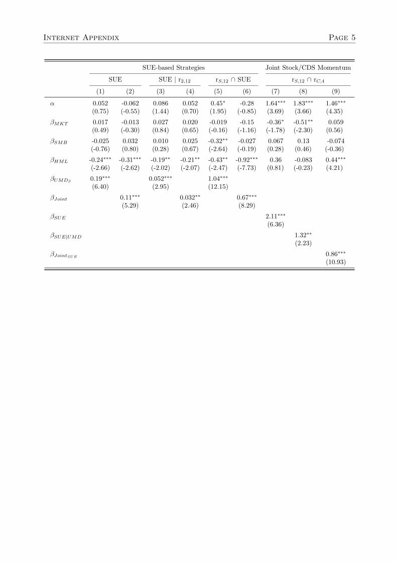
Internet Appendix Page 5
SUE-based Strategies Joint Stock/CDS Momentum
SUE SUE | r2,12 rS,12 ∩ SUE rS,12 ∩ rC,4
(1) (2) (3) (4) (5) (6) (7) (8) (9)
α 0.052 -0.062 0.086 0.052 0.45∗ -0.28 1.64∗∗∗ 1.83∗∗∗ 1.46∗∗∗(0.75) (-0.55) (1.44) (0.70) (1.95) (-0.85) (3.69) (3.66) (4.35)
βMKT 0.017 -0.013 0.027 0.020 -0.019 -0.15 -0.36∗ -0.51∗∗ 0.059(0.49) (-0.30) (0.84) (0.65) (-0.16) (-1.16) (-1.78) (-2.30) (0.56)
βSMB -0.025 0.032 0.010 0.025 -0.32∗∗ -0.027 0.067 0.13 -0.074(-0.76) (0.80) (0.28) (0.67) (-2.64) (-0.19) (0.28) (0.46) (-0.36)
βHML -0.24∗∗∗ -0.31∗∗∗ -0.19∗∗ -0.21∗∗ -0.43∗∗ -0.92∗∗∗ 0.36 -0.083 0.44∗∗∗(-2.66) (-2.62) (-2.02) (-2.07) (-2.47) (-7.73) (0.81) (-0.23) (4.21)
βUMDS 0.19∗∗∗ 0.052∗∗∗ 1.04∗∗∗(6.40) (2.95) (12.15)
βJoint 0.11∗∗∗ 0.032∗∗ 0.67∗∗∗(5.29) (2.46) (8.29)
βSUE 2.11∗∗∗(6.36)
βSUE|UMD 1.32∗∗(2.23)
βJointSUE 0.86∗∗∗(10.93)
Internet Appendix Page 6
D Marginal Information in past CDS Returns using
Various Formation Horizons: Four-Factor Alpha Co-
efficients
This table presents evidence on the marginal information of past CDS returns over mul-
tiple time horizons from one to twelve months. Columns 1 and 2 are strategies based on
unconditional single-market signals. Columns 3 and 4 are strategies based on signals that
are conditioned on the other market’s signal. The conditional strategy is constructed by
creating quintiles of the signal of interest within quintiles of the conditioning signal so that
the top and bottom quintiles are roughly equal with respect to the average value of the
conditioning signal. Each long-short strategy purchases stocks in the top quintile (winners)
and sells short stocks in the bottom quintile (losers). The time period spans January 2003
to December 2015. The 12-lag Newey-West t-statistic is provided in parenthesis, and ∗, ∗∗,
and ∗∗∗ are indicators of statistical significance at the 10%, 5%, and 1% levels, respectively.
Notation for each portfolio return follows the pattern: mean, (t-stat), and annualized Sharpe
ratio.
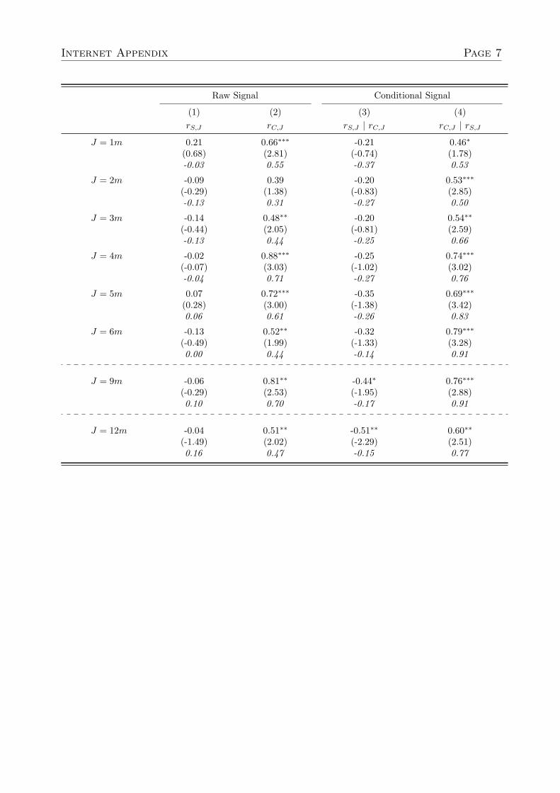
Internet Appendix Page 7
Raw Signal Conditional Signal
(1) (2) (3) (4)rS,J rC,J rS,J | rC,J rC,J | rS,J
J = 1m 0.21 0.66∗∗∗ -0.21 0.46∗(0.68) (2.81) (-0.74) (1.78)-0.03 0.55 -0.37 0.53
J = 2m -0.09 0.39 -0.20 0.53∗∗∗(-0.29) (1.38) (-0.83) (2.85)-0.13 0.31 -0.27 0.50
J = 3m -0.14 0.48∗∗ -0.20 0.54∗∗(-0.44) (2.05) (-0.81) (2.59)-0.13 0.44 -0.25 0.66
J = 4m -0.02 0.88∗∗∗ -0.25 0.74∗∗∗(-0.07) (3.03) (-1.02) (3.02)-0.04 0.71 -0.27 0.76
J = 5m 0.07 0.72∗∗∗ -0.35 0.69∗∗∗(0.28) (3.00) (-1.38) (3.42)0.06 0.61 -0.26 0.83
J = 6m -0.13 0.52∗∗ -0.32 0.79∗∗∗(-0.49) (1.99) (-1.33) (3.28)0.00 0.44 -0.14 0.91
J = 9m -0.06 0.81∗∗ -0.44∗ 0.76∗∗∗(-0.29) (2.53) (-1.95) (2.88)0.10 0.70 -0.17 0.91
J = 12m -0.04 0.51∗∗ -0.51∗∗ 0.60∗∗(-1.49) (2.02) (-2.29) (2.51)0.16 0.47 -0.15 0.77

Internet Appendix Page 8
E Multi-Term Stock Momentum Strategies: Four-Factor
Alpha Coefficients
This table reports alpha coefficients of multi-term stock momentum strategies. The four-
factor model includes the MKT , SMB, HML, and UMDS factors. The multi-term stock
momentum strategy is constructed by double-sorting on the past 12-month stock return and
the past J-month stock return, where J ranges from one to nine months. These strategies
purchase (sell short) stocks that fall in both the 12-month stock winner (loser) portfolio
and the J-month stock winner (loser) portfolio. The time period spans January 2003 to
December 2015. The 12-lag Newey-West t-statistic is provided in parenthesis, and ∗, ∗∗,
and ∗∗∗ are indicators of statistical significance at the 10%, 5%, and 1% levels, respectively.
Notation for each portfolio return follows the pattern: mean, (t-stat), and annualized Sharpe
ratio.

Internet Appendix Page 9
Multi-TermStock Momentum
rS,J ∩ rS,12
J = 1m 0.05(0.08)0.15
J = 2m 0.01(0.03)0.16
J = 3m 0.21(0.89)0.26
J = 4m 0.07(0.33)0.20
J = 5m 0.17(0.82)0.25
J = 6m -0.03(-0.21)0.16
J = 9m -0.21∗(-1.73)0.06

Internet Appendix Page 10
F Factor Exposures of Joint Momentum and Statically
Hedged Joint Momentum
This table shows a more comprehensive list of factor exposures of joint momentum and
statically hedged joint momentum. The joint momentum strategy purchases (sells short)
stocks that are both stock winners (losers) and CDS winners (losers). The statically hedged
joint momentum strategy is 50% invested in joint momentum and 50% invested in a disjoint
contrarian strategy that purchases (sells short) stock losers (winners) that are not CDS
losers (winners). Factors included are the Fama-French three factors (MKT , SMB, HML)
as well as a broad stock market UMD factor and our in-sample UMDS factor. Other
factors include Fama-French five-factor model operating profitability (RMW ) and investment
(CMA) factors, Novy-Marx (2013) gross profitability factor (GPROF ), Asness, Frazzini,
and Pedersen (2014) quality-minus-junk factor (QMJ ), the Stambaugh and Yuan (2016)
mispricing factors (MGMT and PERF ), short-term reversal factor (STREV ), and long-
term reversal factor (LTREV ). The time period spans January 2003 to December 2015. The
12-lag Newey-West t-statistic is provided in parenthesis, and ∗, ∗∗, and ∗∗∗ are indicators of
statistical significance at the 10%, 5%, and 1% levels, respectively.

Internet Appendix Page 11
Panel A. Joint Stock/CDS Momentum
(1) (2) (3) (4) (5) (6) (7) (8)
α 1.67∗∗∗ 1.64∗∗∗ 1.35∗∗∗ 1.51∗∗∗ 1.42∗∗∗ 1.09∗∗∗ 1.45∗∗∗ 1.47∗∗∗(4.08) (2.68) (3.53) (4.31) (3.80) (2.66) (4.15) (4.27)
βMKT -0.15 -0.35∗∗ -0.07 -0.08 -0.06 0.00 -0.08 -0.08(-1.01) (-2.06) (-0.59) (-0.82) (-0.45) (0.02) (-0.74) (-0.70)
βSMB -0.02 0.27 -0.17 -0.18 -0.18 0.26 -0.22 -0.20(-0.12) (0.84) (-1.14) (-1.23) (-1.15) (1.26) (-1.53) (-1.48)
βHML 0.25 -0.61∗∗ 0.11 0.10 0.19 0.16 0.13(1.15) (-2.37) (0.39) (0.46) (0.78) (0.60) (0.53)
βUMD S 0.93∗∗∗ 0.95∗∗∗ 0.94∗∗∗ 0.94∗∗∗ 0.95∗∗∗(10.11) (11.43) (10.44) (11.69) (11.58)
βUMD 1.07∗∗∗(8.46)
βRMW 0.64 0.07(1.46) (0.28)
βCMA 1.02∗ 0.27(1.88) (0.94)
βGPROF -0.14(-0.55)
βQMJ 0.07(0.26)
βMGMT 0.39(1.33)
βPERF 0.99∗∗∗(7.89)
βSTREV 0.12(1.04)
βLTREV 0.16(0.94)
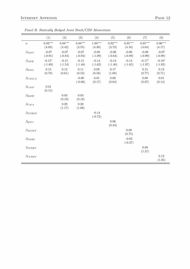
Internet Appendix Page 12
Panel B. Statically Hedged Joint Stock/CDS Momentum
(1) (2) (3) (4) (5) (6) (7) (8)
α 0.93∗∗∗ 0.88∗∗∗ 0.88∗∗∗ 1.00∗∗∗ 0.92∗∗∗ 0.95∗∗∗ 0.95∗∗∗ 0.96∗∗∗(4.03) (3.42) (3.55) (4.30) (3.73) (4.16) (4.04) (4.17)
βMKT -0.07 -0.07 -0.07 -0.08 -0.06 -0.06 -0.08 -0.07(-0.91) (-0.84) (-0.94) (-1.09) (-0.64) (-0.89) (-0.99) (-0.98)
βSMB -0.15∗ -0.15 -0.15 -0.14 -0.14 -0.14 -0.17∗ -0.16∗(-1.89) (-1.54) (-1.48) (-1.62) (-1.40) (-1.65) (-1.97) (-1.92)
βHML 0.15 0.12 0.11 0.08 0.17 0.15 0.13(0.78) (0.61) (0.53) (0.56) (1.00) (0.77) (0.71)
βUMD S -0.00 0.01 0.00 0.00 0.01(-0.06) (0.17) (0.04) (0.07) (0.14)
βUMD 0.01(0.15)
βRMW 0.03 0.03(0.19) (0.19)
βCMA 0.20 0.20(1.17) (1.06)
βGPROF -0.14(-0.72)
βQMJ 0.06(0.34)
βMGMT 0.09(0.75)
βPERF -0.03(-0.27)
βSTREV 0.08(1.21)
βLTREV 0.12(1.05)

Internet Appendix Page 13
References
Asness, Clifford S., Andrea Frazzini, and Lasse H. Pedersen, 2014, Quality minus junk, New
York University Working Paper.
Novy-Marx, Robert, 2013, The other side of value: The gross profitability premium, Journal
of Financial Economics 108, 1–28.
Stambaugh, Robert F., and Yu Yuan, 2016, Mispricing factors, Review of Financial Studies,
forthcoming.