relating phase field and sharp interface approaches...

Weierstrass Institute forApplied Analysis and Stochastics

Relating phase field and sharp interface

approaches to structural topology optimization

M.Hassan Farshbaf Shaker

joint work with: L. Blank, H. Garcke (Regensburg), V. Styles (Sussex)

Mohrenstrasse 39 · 10117 Berlin · Germany · Tel. +49 30 20372 0 · www.wias-berlin.de

SADCO-WIAS Young Research Workshop 2014, January 29-31, Berlin

Content

1 Introduction into structural topology optimization

2 Multi-material phase field approach

3 Sharp interface limit of the phase field approximation

4 Numerics

M. Hassan Farshbaf-Shaker · SADCO-WIAS Young Research Workshop 2014, January 29-31, Berlin · (32)




4 Numerics


Problemsetting in structural topology optimization

Domain Ω to be designed:

1. solid domain ΩM with

fixed given volume

|ΩM | = m

2. void Ω \ ΩM

Volume forces f given

Surface loads g, Traction forces

given

Aim of the structural topology optimization:

Distribute a limited amount of material ΩM in a design domain Ω such that an objective

functional J is minimized.


Problemsetting in structural topology optimization

Domain Ω to be designed:

1. solid domain ΩM with

fixed given volume

|ΩM | = m

2. void Ω \ ΩM

Volume forces f given

Surface loads g, Traction forces

given

Aim of the structural topology optimization:

Distribute a limited amount of material ΩM in a design domain Ω such that an objective

functional J is minimized.

M. Hassan Farshbaf-Shaker · SADCO-WIAS Young Research Workshop 2014, January 29-31, Berlin ·Page 4 (32)

Structural topology optimization

Mathematical formulation:

Given a design domain Ω ⊂ Rd and m

minΩM∈Uad

J(ΩM )

Admissible set: Uad = ΩM ⊂ Ω such that |ΩM | = m

Solve simultaneously the elasticity equation (solid domain modeled as linear elastic

material)

−div(CME(u)) = f in ΩM and boundary conditions

elasticity tensor CM

linearized strain tensor E(u) = 12(∇u+∇uT )

Displacement field u


Possible objective functionals

First choice

Maximize stiffness or equivalently Minimize compliance (work done by the load)

J1(ΩM ) =

∫ΩM

f · u+

∫Γg

g · u .

Concrete examples for mean compliance

Michell type structure Cantilever beam configuration


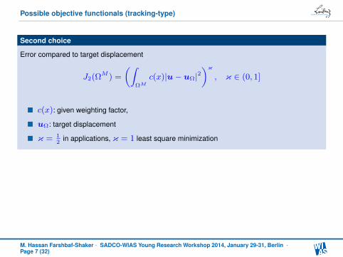
Possible objective functionals (tracking-type)

Second choice

Error compared to target displacement

J2(ΩM ) =

(∫ΩM

c(x)|u− uΩ|2)κ

, κ ∈ (0, 1]

c(x): given weighting factor,

uΩ: target displacement

κ = 12

in applications, κ = 1 least square minimization

Concrete example for compliant mechanism

Minimize error to given

target displacementPush configuration


Possible objective functionals

Structural optimization problem

Minimize J(ΩM ) = αJ1(ΩM ) + βJ2(ΩM ) subject to

−div(CME(u)) = f in ΩM

(CME(u))n = 0 on Γ0

(CME(u))n = g on Γg

u = 0 on ΓD

Problem is not well-posed !

A possible path to well-posedness

Add the perimeter: P (ΩM ) =∫

(∂ΩM )∩Ωds:

J(ΩM ) = αJ1(ΩM ) + βJ2(ΩM ) + γP (ΩM )


Approaches used to tackle structural optimization problems

Classical method of shape calculus: Boundary variations based on a parametric approach

drawbacks: topology changes difficult / serious remeshing necessary

Homogenization methods and variants of it (Allaire, Bendsoe, Sigmund and many others)

(power law materials, Solid Isotropic Material with Penalization (SIMP) method)

Applicability restricted to particular objective functionals

Level set methods (Sethian, Osher, Allaire, Burger and many others)

(Applicable to a wide range of problems)

drawbacks: difficult to create holes / (topological derivatives would help)





4 Numerics


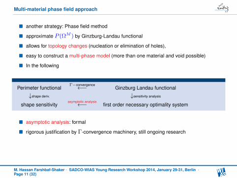
Multi-material phase field approach

another strategy: Phase field method

approximate P (ΩM ) by Ginzburg-Landau functional

allows for topology changes (nucleation or elimination of holes),

easy to construct a multi-phase model (more than one material and void possible)

In the following

Perimeter functionalΓ−convergence←− Ginzburg Landau functional

↓shape deriv. ↓sensitivity analysis

shape sensitivityasymptotic analysis←− first order necessary optimality system

asymptotic analysis: formal

rigorous justification by Γ-convergence machinery, still ongoing research


Phase field approach, earlier work

B. Bourdin, A. Chambolle, Design-dependent loads in topology optimization, ESAIM Contr. Optim. Calc. Var. 9 (2003) 19-48.

M.Y. Wang, S.W. Zhou, Phase field: A variational method for structural topology optimization. Comput. Model. Eng. Sci. 6(2004)547-566.

B. Bourdin, A. Chambolle, The phase field method in optimal design, in: IUTAM Symposium on Topological Design Optimization ofStructures, Machines and Materials (2006) 207-215.

M. Burger, R. Stainko, Phase field relaxation of topology optimization with local stress constraints. SIAM J. Control Optim. 45 (2006)1447-1466.

L. Blank, H. Garcke, L. Sarbu, T. Srisupattarawanit, V. Styles, A. Voigt, Phase field approaches to structural topology optimization. 2010(to be published in: K.H. Hoffmann and G. Leugering (Eds.): Optimization with Partial Differential Equations, ISNM, Birkhäuser Verlag)

A. Takezawa, S. Nishiwaki, M. Kitamura, Shape and topology optimization based on the phase field method and sensitivity analysis.Journal of Computational Physics 229 (7) (2010), 2697-2718.

P. Penzler, M. Rumpf, B. Wirth, A phase field model for compliance shape optimization in nonlinear elasticity, ESAIM Control Optim.Calc. Var. 18 (2012), no. 1, 229-258.

Common: focus on numerical aspects and formal analysis,


Phase field approach: Introduction

phase field ϕ := (ϕi)Ni=1; phase-fraction ϕi; void ϕN ; ε > 0 interface width

Gibbs-SimplexG = v ∈ RN | vi ≥ 0,∑Ni=1 vi = 1

G := v ∈ H1(Ω,RN ) | v(x) ∈ G a.e. in Ω Gm := v ∈ G |

∫Ω− v = m

Exapmle: 3 materials





G := v ∈ H1(Ω,RN ) | v(x) ∈ G a.e. in Ω

Gm := v ∈ G |∫

Ω− v = m






G := v ∈ H1(Ω,RN ) | v(x) ∈ G a.e. in Ω Gm := v ∈ G |

∫Ω− v = m




mechanical properties of the system

linear elasticity

elasticity tensors in material for each phase Ci, i ∈ 1, . . . , N − 1

void is modeled as a very soft ”ersatz material” with a very small elasticity tensor

CN = CN (ε) = ε2CN

(quadratic rate in ε accelerates the convergence in the void as ε→ 0 and is hence

chosen in the numerical computations)

elasticity tensor in the interfacial region: C(ϕ) = C(ϕ) + CN (ε)ϕN , ∀ϕ ∈ G,

C(ϕ) :=N−1∑i=1

Ciϕi



mechanical properties of the system

linear elasticity

elasticity tensors in material for each phase Ci, i ∈ 1, . . . , N − 1 void is modeled as a very soft ”ersatz material” with a very small elasticity tensor

CN = CN (ε) = ε2CN

(quadratic rate in ε accelerates the convergence in the void as ε→ 0 and is hence

chosen in the numerical computations)

elasticity tensor in the interfacial region: C(ϕ) = C(ϕ) + CN (ε)ϕN , ∀ϕ ∈ G,

C(ϕ) :=N−1∑i=1

Ciϕi


Phase field approach

Ginzburg-Landau functional

Eε(ϕ) :=

∫Ω

(ε

2|∇ϕ|2 +

1

εΨ(ϕ)

)dx, ε > 0,

Prototype examples for Ψ are given by

Ψ(ϕ) :=1

2(1−ϕ ·ϕ) and Ψ(ϕ) :=

1

2ϕ · Wϕ

mean complinace J1 and compliant mechanism J2

J1(u,ϕ) =

∫Ω

(1− ϕN )f · u+

∫Γg

g · u,

J2(u,ϕ) :=

(∫Ω

c (1− ϕN )|u− uΩ|2)κ

, κ ∈ (0, 1]


Similarities to optimal control problem, control: ϕ, state: u

(Pε)

min Jε(u,ϕ) := αJ1(u,ϕ) + βJ2(u,ϕ) + γEε(ϕ),

over (u,ϕ) ∈ H1D(Ω,Rd)×H1(Ω,RN ),

s.t. (SE)

−∇ · [C(ϕ)E(u)] =

(1− ϕN

)f in Ω,

u = 0 on ΓD,

[C(ϕ)E(u)]n = g on Γg,

[C(ϕ)E(u)]n = 0 on Γ0,

ϕ ∈ Gm ∩U c,

U c := ϕ ∈ H1(Ω,RN ) | ϕN = 0 a.e. on S0 and ϕN = 1 a.e. on S1.

Gm := v ∈ G |∫

Ω− v = m, G := v ∈ H1(Ω,RN ) | v(x) ∈ G a.e. in Ω,

G = v ∈ RN | vi ≥ 0,∑Ni=1 vi = 1


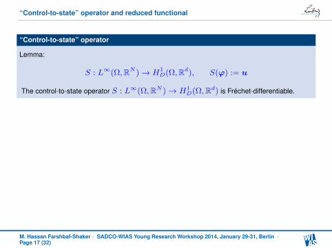
“Control-to-state” operator and reduced functional

“Control-to-state” operator

Lemma:

S : L∞(Ω,RN )→ H1D(Ω,Rd), S(ϕ) := u

The control-to-state operator S : L∞(Ω,RN )→ H1D(Ω,Rd) is Fréchet-differentiable.

Reduced cost-functional

Lemma:

j(ϕ) := Jε(S(ϕ),ϕ) = αJ1(S(ϕ),ϕ) + βJ2(S(ϕ),ϕ) + γEε(ϕ)

The reduced cost-functional j : H1(Ω,RN ) ∩ L∞(Ω,RN )→ R is Fréchet-differentiable.


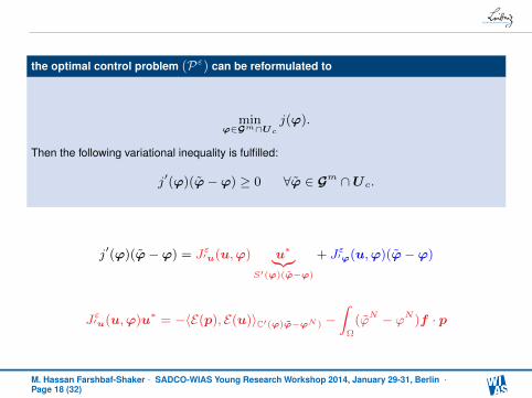
the optimal control problem (Pε) can be reformulated to

minϕ∈Gm∩Uc

j(ϕ).

Then the following variational inequality is fulfilled:

j′(ϕ)(ϕ−ϕ) ≥ 0 ∀ϕ ∈ Gm ∩U c.

j′(ϕ)(ϕ−ϕ) = Jε′u(u,ϕ) u∗︸︷︷︸S′(ϕ)(ϕ−ϕ)

+ Jε′ϕ(u,ϕ)(ϕ−ϕ)

Jε′u(u,ϕ)u∗ = −〈E(p), E(u)〉C′(ϕ)ϕ−ϕN ) −∫

Ω

(ϕN − ϕN )f · p


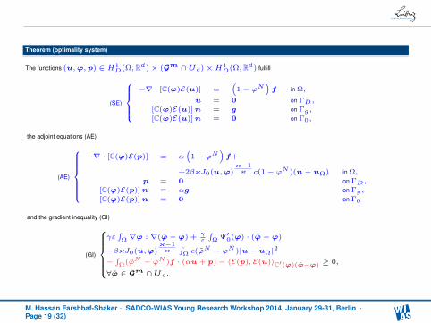
Theorem (optimality system)

The functions (u,ϕ,p) ∈ H1D(Ω,Rd)× (Gm ∩Uc)×H1

D(Ω,Rd) fulfill

(SE)

−∇ · [C(ϕ)E(u)] =

(1− ϕN

)f in Ω,

u = 0 on ΓD,

[C(ϕ)E(u)]n = g on Γg,

[C(ϕ)E(u)]n = 0 on Γ0,

the adjoint equations (AE)

(AE)

−∇ · [C(ϕ)E(p)] = α(1− ϕN

)f+

+2βκJ0(u,ϕ)κ−1κ c(1− ϕN )(u− uΩ) in Ω,

p = 0 on ΓD,

[C(ϕ)E(p)] n = αg on Γg,

[C(ϕ)E(p)]n = 0 on Γ0

and the gradient inequality (GI)

(GI)

γε∫Ω∇ϕ : ∇(ϕ− ϕ) + γ

ε

∫Ω Ψ′0(ϕ) · (ϕ− ϕ)

−βκJ0(u,ϕ)κ−1κ

∫Ω c(ϕ

N − ϕN )|u− uΩ|2

−∫Ω(ϕN − ϕN )f · (αu + p)− 〈E(p), E(u)〉C′(ϕ)(ϕ−ϕ) ≥ 0,

∀ϕ ∈ Gm ∩Uc.





4 Numerics


Asymptotic expansion

Interfacial regions have thickness ε

Structure of phase field across interface

Use rescaled variable z =dist(x,ϕε=

12)

ε

Matched asymptotic expansions


Sharp interface limit as ε→ 0

Domain Ω is partitioned into N regions

Ωi separated by interfaces Γij ,

[w]ji jump across interface.

We obtain for i, j ∈ 1, . . . , N − 1: (material-material)

(SE)i

−∇ ·

[CiE(u)

]= f in Ωi,

[u]ji = 0 on Γij ,

[CE(u)ν]ji = 0 on Γij ,

(AE)i

−∇ ·

[CiE(p)

]= αf + 2βκJ0(u,ϕ)

κ−1κ c(u− uΩ) in Ωi,

[p]ji = 0 on Γij ,

[CE(p)ν]ji = 0 on Γij ,

and we have (CiEi(u))ν = (CiEi(p))ν = 0 on ΓiN (material-void).


Sharp interface limit as ε→ 0

For all i, j 6= N (material-material) interface

0 = γσijκ−[CE(u) : E(p)]ji + [CE(u)ν · (∇p)ν]ji

+[CE(p)ν · (∇u)ν]ji−[λ1]ji

Term−[CE(u) : E(p)]ji + [CE(u)ν · (∇p)ν]ji + [CE(p)ν · (∇u)ν]ji generalizes the

Eshelby traction (compare materials science)

0 = γσiNκ+ CiEi(u) : Ei(p)

−βκJ0(u,ϕ)κ−1κ c |u− uΩ|2 − f · (αu+ p) + (λ1)i − (λ1)N .

(void-material) interface


Choose angle at triple junction

Example computation

Typically angles at void should be 180 or

close to it (otherwise cracks are possible)

Angles in phase field model are determined

by energy Ψ (Bronsard, Reitich; Bronsard,

Garcke, Stoth)

Important: Asymptotic analysis shows

elasticity does not influence equilibrium

angles possible configuration at triple

junction





4 Numerics


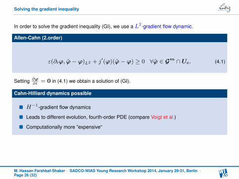
Solving the gradient inequality

In order to solve the gradient inequality (GI), we use a L2-gradient flow dynamic.

Allen-Cahn (2.order)

ε(∂tϕ, ϕ−ϕ)L2 + j′(ϕ)(ϕ−ϕ) ≥ 0 ∀ϕ ∈ Gm ∩Uc. (4.1)

Setting ∂ϕ∂t

= 0 in (4.1) we obtain a solution of (GI).

Cahn-Hilliard dynamics possible

H−1-gradient flow dynamics

Leads to different evolution, fourth-order PDE (compare Voigt et al.)

Computationally more ”expensive“


Numerical solution techniques

finite element approximation of ϕ,u,p

semi-implicit in time: pseudo-time stepping approach to gradient inequality

solve variational inequality with primal dual active set method (PDAS) (Hintermüller, Ito,

Kunisch)

Analyzed for Cahn-Hilliard variational inequality by Blank, Butz, Garcke

Analyzed for Allen–Cahn systems by Blank, Garcke, Sarbu, Styles

More efficient methods for the overall optimization problem Blank, Rupprecht

H1-gradient projection and SQP method


Michell construction d = 2, N = 2, β = 0 (red: material, blue: void)

Deformed state

. . . . . . . . . . . . . . . . . . . . . . . . . . . . . . . . . . . . . . . . . . . . . . . . . . . . . . . . . . . . . . . . . . . . . . . . . . . . . . . . . . . . . . . . . . . . . . .

t = 0.0 t = 0.0002 t = 0.0003

t = 0.0005 t = 0.001 t = 0.006

Typical computation starting with checker-board Topology changes


Cantilever beam construction d = 2, N = 3, β = 0

Here: two materials and void

Deformed state

. . . . . . . . . . . . . . . . . . . . . . . . . . . . . . . . . . . . . . . . . . . . . . . . . . . . . . . . . . . . . . . . . . . . . . . . . . . . . . . . . . . . . . . . . . . . . . .

t = 0.000 t = 0.0015 t = 0.01

t = 0.02 t = 0.04 t = 0.3

(red: hard material, green: soft material, blue: void )


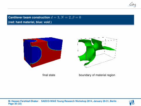
Cantilever beam construction d = 3, N = 2, β = 0

(red: hard material, blue: void )

final state boundary of material region


Push construction (red: material, blue: void)

t=0.0 t = 0.004 t = 0.01

t=0.02 t = 0.035 t = 2.25Computation of adjoint state necessary


Summary / Conclusions

Introduced a phase field method for multi-material structural topology optimization

(based on earlier work by Bourdin/Chambolle, Wang/Zhou, Burger/Stainko)

First order optimality conditions were rigorously derived

Sharp interface limit was analyzed with the help of formally matched asymptotic

expansions

In the limit we obtained classical shape derivatives and some new shape derivatives for

the multi-material situation

With the help of asymptotics at the triple junction

Numerical computations demonstrated the applicability of the approach

L. Blank, M.H. Farshbaf-Shaker, H. Garcke, V. Styles, Relating phase field and sharp

interface approaches to structural topology optimization. to be published in ESAIM Contr.

Optim. Calc. Var.

Thank you for your Attention!


relating phase field and sharp interface approaches...

Documents