relational database design and multi-objective database
TRANSCRIPT

Air Force Institute of Technology Air Force Institute of Technology
AFIT Scholar AFIT Scholar
Theses and Dissertations Student Graduate Works
3-26-2020
Relational Database Design and Multi-Objective Database Queries Relational Database Design and Multi-Objective Database Queries
for Position Navigation and Timing Data for Position Navigation and Timing Data
Sean A. Mochocki
Follow this and additional works at: https://scholar.afit.edu/etd
Part of the Databases and Information Systems Commons, and the Navigation, Guidance, Control and
Dynamics Commons
Recommended Citation Recommended Citation Mochocki, Sean A., "Relational Database Design and Multi-Objective Database Queries for Position Navigation and Timing Data" (2020). Theses and Dissertations. 3184. https://scholar.afit.edu/etd/3184
This Thesis is brought to you for free and open access by the Student Graduate Works at AFIT Scholar. It has been accepted for inclusion in Theses and Dissertations by an authorized administrator of AFIT Scholar. For more information, please contact [email protected].

RELATIONAL DATABASE DESIGN ANDMULTI-OBJECTIVE DATABASE QUERIES
FOR POSITION NAVIGATION AND TIMINGDATA
THESIS
Sean A. Mochocki, Captain, USAF
AFIT-ENG-MS-20-M-045
DEPARTMENT OF THE AIR FORCEAIR UNIVERSITY
AIR FORCE INSTITUTE OF TECHNOLOGY
Wright-Patterson Air Force Base, Ohio
DISTRIBUTION STATEMENT AAPPROVED FOR PUBLIC RELEASE; DISTRIBUTION UNLIMITED.

The views expressed in this document are those of the author and do not reflect theofficial policy or position of the United States Air Force, the United States Departmentof Defense or the United States Government. This material is declared a work of theU.S. Government and is not subject to copyright protection in the United States.
AFIT-ENG-MS-20-M-045
RELATIONAL DATABASE DESIGN AND MULTI-OBJECTIVE DATABASE
QUERIES FOR POSITION NAVIGATION AND TIMING DATA
THESIS
Presented to the Faculty
Department of Electrical and Computer Engineering
Graduate School of Engineering and Management
Air Force Institute of Technology
Air University
Air Education and Training Command
in Partial Fulfillment of the Requirements for the
Degree of Master of Science in Computer Science
Sean A. Mochocki, B.S.E.E., B.S.M.E.
Captain, USAF
March 2020
DISTRIBUTION STATEMENT AAPPROVED FOR PUBLIC RELEASE; DISTRIBUTION UNLIMITED.
AFIT-ENG-MS-20-M-045
RELATIONAL DATABASE DESIGN AND MULTI-OBJECTIVE DATABASE
QUERIES FOR POSITION NAVIGATION AND TIMING DATA
THESIS
Sean A. Mochocki, B.S.E.E., B.S.M.E.Captain, USAF
Committee Membership:
Robert C Leishman, Ph.D.Chair
Kyle J Kauffman, Ph.D.Member
John F Raquet, Ph.D.Member
AFIT-ENG-MS-20-M-045
Abstract
Performing flight tests is a natural part of researching cutting edge sensors and filters
for sensor integration. Unfortunately, tests are expensive, and typically take many
months of planning. A sensible goal would be to make previously collected data
readily available to researchers for future development.
The Air Force Institute of Technology (AFIT) has hundreds of data logs poten-
tially available to aid in facilitating further research in the area of navigation. A
database would provide a common location where older and newer data sets are
available. Such a database must be able to store the sensor data, metadata about the
sensors, and affiliated metadata of interest.
This thesis proposes a standard approach for sensor and metadata schema and
three different design approaches that organize this data in relational databases.
Queries proposed by members of the Autonomy and Navigation Technology (ANT)
Center at AFIT are the foundation of experiments for testing. These tests fall into
two categories, downloaded data, and queries which return a list of missions. Test
databases of 100 and 1000 missions are created for the three design approaches to
simulate AFIT’s present and future volume of data logs. After testing, this thesis
recommends one specific approach to the ANT Center as its database solution.
In order to enable more complex queries, a Genetic algorithm and Hill Climber
algorithm are developed as solutions to queries in the combined Knapsack/Set Cov-
ering Problem Domains. These algorithms are tested against the two test databases
for the recommended database approach. Each algorithm returned solutions in under
two minutes, and may be a valuable tool for researchers when the database becomes
operational.
iv
Table of Contents
Page
Abstract . . . . . . . . . . . . . . . . . . . . . . . . . . . . . . . . . . . . . . . . . . . . . . . . . . . . . . . . . . . . . . . iv
List of Figures . . . . . . . . . . . . . . . . . . . . . . . . . . . . . . . . . . . . . . . . . . . . . . . . . . . . . . . . . viii
List of Tables . . . . . . . . . . . . . . . . . . . . . . . . . . . . . . . . . . . . . . . . . . . . . . . . . . . . . . . . . . . xi
List of Acronyms . . . . . . . . . . . . . . . . . . . . . . . . . . . . . . . . . . . . . . . . . . . . . . . . . . . . . . . xiv
I. Introduction . . . . . . . . . . . . . . . . . . . . . . . . . . . . . . . . . . . . . . . . . . . . . . . . . . . . . . . . 1
1.1 Background and Motivation . . . . . . . . . . . . . . . . . . . . . . . . . . . . . . . . . . . . . . 11.2 Problem Background. . . . . . . . . . . . . . . . . . . . . . . . . . . . . . . . . . . . . . . . . . . . . 21.3 Design Objectives and Characteristics . . . . . . . . . . . . . . . . . . . . . . . . . . . . . . 2
II. Background and Related Work . . . . . . . . . . . . . . . . . . . . . . . . . . . . . . . . . . . . . . . . 4
2.1 Overview . . . . . . . . . . . . . . . . . . . . . . . . . . . . . . . . . . . . . . . . . . . . . . . . . . . . . . . 42.2 Position Navigation and Timing Data . . . . . . . . . . . . . . . . . . . . . . . . . . . . . . 4
2.2.1 Scorpion Data Model . . . . . . . . . . . . . . . . . . . . . . . . . . . . . . . . . . . . . . 52.2.2 YAML Ain’t Markup Language . . . . . . . . . . . . . . . . . . . . . . . . . . . . . 62.2.3 Lightweight Communications and Marshalling . . . . . . . . . . . . . . . . . 6
2.3 Big Data Overview . . . . . . . . . . . . . . . . . . . . . . . . . . . . . . . . . . . . . . . . . . . . . . 72.3.1 Definitions of Big Data . . . . . . . . . . . . . . . . . . . . . . . . . . . . . . . . . . . . . 82.3.2 Five V Model . . . . . . . . . . . . . . . . . . . . . . . . . . . . . . . . . . . . . . . . . . . . . 9
2.4 Data Modeling . . . . . . . . . . . . . . . . . . . . . . . . . . . . . . . . . . . . . . . . . . . . . . . . . 122.5 Relational Databases . . . . . . . . . . . . . . . . . . . . . . . . . . . . . . . . . . . . . . . . . . . 14
2.5.1 Normalization . . . . . . . . . . . . . . . . . . . . . . . . . . . . . . . . . . . . . . . . . . . . 152.5.2 Entity Relationship Diagrams . . . . . . . . . . . . . . . . . . . . . . . . . . . . . . 162.5.3 Structured Query Language . . . . . . . . . . . . . . . . . . . . . . . . . . . . . . . . 172.5.4 SQLite . . . . . . . . . . . . . . . . . . . . . . . . . . . . . . . . . . . . . . . . . . . . . . . . . . 182.5.5 PostgreSQL . . . . . . . . . . . . . . . . . . . . . . . . . . . . . . . . . . . . . . . . . . . . . 18
2.6 Non-Relational Databases . . . . . . . . . . . . . . . . . . . . . . . . . . . . . . . . . . . . . . . 182.6.1 The Consistent, Available, or Partition Tolerant
Theorem . . . . . . . . . . . . . . . . . . . . . . . . . . . . . . . . . . . . . . . . . . . . . . . . 192.6.2 Basically Available, Soft state, Eventual
consistency Properties . . . . . . . . . . . . . . . . . . . . . . . . . . . . . . . . . . . . . 212.6.3 Standard Types of Not only SQL Databases . . . . . . . . . . . . . . . . . . 22
2.7 Data Warehouses, OLTPs and OLAPs . . . . . . . . . . . . . . . . . . . . . . . . . . . . 242.8 NewSQL . . . . . . . . . . . . . . . . . . . . . . . . . . . . . . . . . . . . . . . . . . . . . . . . . . . . . . 252.9 Multi-Objective Database Queries . . . . . . . . . . . . . . . . . . . . . . . . . . . . . . . . 262.10 Cloud Computing . . . . . . . . . . . . . . . . . . . . . . . . . . . . . . . . . . . . . . . . . . . . . . 272.11 Relevant Research . . . . . . . . . . . . . . . . . . . . . . . . . . . . . . . . . . . . . . . . . . . . . . 28
v

Page
2.12 Summary . . . . . . . . . . . . . . . . . . . . . . . . . . . . . . . . . . . . . . . . . . . . . . . . . . . . . 29
III. Design . . . . . . . . . . . . . . . . . . . . . . . . . . . . . . . . . . . . . . . . . . . . . . . . . . . . . . . . . . . . 32
3.1 ION/PLANS Paper Introduction . . . . . . . . . . . . . . . . . . . . . . . . . . . . . . . . . 323.2 Relevant Background . . . . . . . . . . . . . . . . . . . . . . . . . . . . . . . . . . . . . . . . . . . 33
3.2.1 PNT Database Characteristics . . . . . . . . . . . . . . . . . . . . . . . . . . . . . 343.2.2 Relational Databases . . . . . . . . . . . . . . . . . . . . . . . . . . . . . . . . . . . . . . 353.2.3 Non-Relational Databases . . . . . . . . . . . . . . . . . . . . . . . . . . . . . . . . . 373.2.4 Database Decision Summary . . . . . . . . . . . . . . . . . . . . . . . . . . . . . . . 39
3.3 Database Designs . . . . . . . . . . . . . . . . . . . . . . . . . . . . . . . . . . . . . . . . . . . . . . . 403.3.1 Requirements and Approaches . . . . . . . . . . . . . . . . . . . . . . . . . . . . . 403.3.2 Table and Relationship Descriptions . . . . . . . . . . . . . . . . . . . . . . . . 41
3.4 Design of Experiments . . . . . . . . . . . . . . . . . . . . . . . . . . . . . . . . . . . . . . . . . . 483.4.1 Database Population . . . . . . . . . . . . . . . . . . . . . . . . . . . . . . . . . . . . . . 483.4.2 Test Designs . . . . . . . . . . . . . . . . . . . . . . . . . . . . . . . . . . . . . . . . . . . . . 493.4.3 Expected Performance . . . . . . . . . . . . . . . . . . . . . . . . . . . . . . . . . . . . 533.4.4 Test Procedures . . . . . . . . . . . . . . . . . . . . . . . . . . . . . . . . . . . . . . . . . . 53
3.5 Test Results . . . . . . . . . . . . . . . . . . . . . . . . . . . . . . . . . . . . . . . . . . . . . . . . . . . 553.5.1 Download Test Results Summary . . . . . . . . . . . . . . . . . . . . . . . . . . . 553.5.2 SDM Query Test Results Summary . . . . . . . . . . . . . . . . . . . . . . . . . 57
3.6 Conclusion . . . . . . . . . . . . . . . . . . . . . . . . . . . . . . . . . . . . . . . . . . . . . . . . . . . . 613.7 Database Population . . . . . . . . . . . . . . . . . . . . . . . . . . . . . . . . . . . . . . . . . . . . 63
3.7.1 Log File Ordering . . . . . . . . . . . . . . . . . . . . . . . . . . . . . . . . . . . . . . . . 633.7.2 Non-Sensor Metadata Insertion Algorithms . . . . . . . . . . . . . . . . . . 643.7.3 insertChannelInformation Function . . . . . . . . . . . . . . . . . . . . . . . . . 653.7.4 insertRandomSensorMetadata . . . . . . . . . . . . . . . . . . . . . . . . . . . . . . 663.7.5 insertSDMData . . . . . . . . . . . . . . . . . . . . . . . . . . . . . . . . . . . . . . . . . . 68
3.8 Indexes . . . . . . . . . . . . . . . . . . . . . . . . . . . . . . . . . . . . . . . . . . . . . . . . . . . . . . . 723.9 Removed Metadata Query Test Figures . . . . . . . . . . . . . . . . . . . . . . . . . . . . 73
IV. Experimental Scenarios . . . . . . . . . . . . . . . . . . . . . . . . . . . . . . . . . . . . . . . . . . . . . 76
4.1 Journal Of Evolutionary Computation Paper . . . . . . . . . . . . . . . . . . . . . . . 764.2 Background and Related Queries . . . . . . . . . . . . . . . . . . . . . . . . . . . . . . . . . 784.3 Problem Domain . . . . . . . . . . . . . . . . . . . . . . . . . . . . . . . . . . . . . . . . . . . . . . . 83
4.3.1 Set Covering Problem . . . . . . . . . . . . . . . . . . . . . . . . . . . . . . . . . . . . . 834.3.2 The Knapsack Problem . . . . . . . . . . . . . . . . . . . . . . . . . . . . . . . . . . . 844.3.3 Combined Problem . . . . . . . . . . . . . . . . . . . . . . . . . . . . . . . . . . . . . . . 85
4.4 Stochastic Algorithms for the Combined MO KP/SCP . . . . . . . . . . . . . . 884.4.1 Genetic Algorithm . . . . . . . . . . . . . . . . . . . . . . . . . . . . . . . . . . . . . . . . 884.4.2 Hill Climber Algorithm . . . . . . . . . . . . . . . . . . . . . . . . . . . . . . . . . . . . 924.4.3 GA and HC Algorithm Expected Performance . . . . . . . . . . . . . . . . 93
4.5 Design and Evaluation of Experiments . . . . . . . . . . . . . . . . . . . . . . . . . . . . 95
vi

Page
4.6 Conclusion . . . . . . . . . . . . . . . . . . . . . . . . . . . . . . . . . . . . . . . . . . . . . . . . . . . . 98
V. Conclusion . . . . . . . . . . . . . . . . . . . . . . . . . . . . . . . . . . . . . . . . . . . . . . . . . . . . . . . 102
Appendix A. Full Database Schema . . . . . . . . . . . . . . . . . . . . . . . . . . . . . . . . . . . . . . 106
Appendix B. Tester Questionnaire . . . . . . . . . . . . . . . . . . . . . . . . . . . . . . . . . . . . . . . 111
Appendix C. Database Test Results . . . . . . . . . . . . . . . . . . . . . . . . . . . . . . . . . . . . . 114
Appendix D. KP/SCP GA Results . . . . . . . . . . . . . . . . . . . . . . . . . . . . . . . . . . . . . . 129
Appendix E. SQL Queries . . . . . . . . . . . . . . . . . . . . . . . . . . . . . . . . . . . . . . . . . . . . . . 133
Appendix F. SQL Database and Index Scripts . . . . . . . . . . . . . . . . . . . . . . . . . . . . 144
Appendix G. Genetic Algorithm Pseudo Code . . . . . . . . . . . . . . . . . . . . . . . . . . . . . 165
Appendix H. Hill Climber Pseudo Code . . . . . . . . . . . . . . . . . . . . . . . . . . . . . . . . . . 168
Appendix I. Proof that KP/SCP Decision Problem isNP-Complete . . . . . . . . . . . . . . . . . . . . . . . . . . . . . . . . . . . . . . . . . . . . . 170
Bibliography . . . . . . . . . . . . . . . . . . . . . . . . . . . . . . . . . . . . . . . . . . . . . . . . . . . . . . . . . . 173
vii

List of Figures
Figure Page
1. Big Data use in Social Media [1] . . . . . . . . . . . . . . . . . . . . . . . . . . . . . . . . . . . 8
2. The Four V’s of Big Data [2] . . . . . . . . . . . . . . . . . . . . . . . . . . . . . . . . . . . . . 11
3. The Five Vs of Big Data [3] . . . . . . . . . . . . . . . . . . . . . . . . . . . . . . . . . . . . . . 12
4. The Consistent, Available, or Partition Tolerant (CAP)theorem visualized [4] . . . . . . . . . . . . . . . . . . . . . . . . . . . . . . . . . . . . . . . . . . . 20
5. OLAP vs OLTP [5] . . . . . . . . . . . . . . . . . . . . . . . . . . . . . . . . . . . . . . . . . . . . . 25
6. Cloud Computing Services [6] . . . . . . . . . . . . . . . . . . . . . . . . . . . . . . . . . . . . 29
7. Relational PNT Database Overview For All DesignApproaches . . . . . . . . . . . . . . . . . . . . . . . . . . . . . . . . . . . . . . . . . . . . . . . . . . . . 42
8. Primary File Download Test: Lower times indicate abetter performance. Each test was performed 11 timesfor each approach and database. . . . . . . . . . . . . . . . . . . . . . . . . . . . . . . . . . . 56
9. Trim By Altitude Test: Lower times indicate a betterperformance. Each test was performed 11 times for eachapproach and database. . . . . . . . . . . . . . . . . . . . . . . . . . . . . . . . . . . . . . . . . . . 56
10. Trim By Velocity Test: Lower times indicate a betterperformance. Each test was performed 11 times for eachapproach and database. . . . . . . . . . . . . . . . . . . . . . . . . . . . . . . . . . . . . . . . . . . 56
11. Trim By Time Cut Beginning Test: Lower timesindicate a better performance. Each test was performed11 times for each approach and database. . . . . . . . . . . . . . . . . . . . . . . . . . . 57
12. Trim By Time Cut Ending Test: Lower times indicate abetter performance. Each test was performed 11 timesfor each approach and database. . . . . . . . . . . . . . . . . . . . . . . . . . . . . . . . . . . 57
13. Platform Dynamics Test: Queries the IMU data type tocheck for High (4 g’s) Medium (Between 4 and 2 g’s) orLow (Less than 2 g’s) dynamics. Each test wasperformed 11 times for each approach and database . . . . . . . . . . . . . . . . . 59
viii

Figure Page
14. Time Of Day Test: Queries the IMU data type to checkfor if the data log began in the morning, or ended in theafternoon, Eastern Standard Time. Each test wasperformed 11 times for each approach and database . . . . . . . . . . . . . . . . . 59
15. Velocity Test: Queries the PositionVelocityAttitudetable to see if a data log exceeded 5m/s in anydirection. Each test was performed 11 times for eachapproach and database . . . . . . . . . . . . . . . . . . . . . . . . . . . . . . . . . . . . . . . . . . 59
16. Satellite Type Test: Queries the GNSS table to see if arandomly chosen satellite constellation provided ameasurement for that data log. Each test wasperformed 11 times for each approach and database . . . . . . . . . . . . . . . . . 60
17. Latitude Longitude Bounding Test: Checks theGeodeticPosition 3D table to see if any measurementin the data log took place within a certain Latitude andLongitude. Each test was performed 11 times for eachapproach and database . . . . . . . . . . . . . . . . . . . . . . . . . . . . . . . . . . . . . . . . . . 60
18. Sensor Quality Test Results: Runs queries whichidentify which data logs which used a IMU sensor havespecified intrinsic values. Each test was performed 11times for each approach and database . . . . . . . . . . . . . . . . . . . . . . . . . . . . . 61
19. Non-Sensor Metadata Queries Result: Runs queriesconcerning Weather, Terrain, and Maneuvers. Each testwas performed 11 times for each approach and database . . . . . . . . . . . . . 74
20. Vehicle Queries Results: Runs various Vehicle relatedqueries. Each test was performed 11 times for eachapproach and database . . . . . . . . . . . . . . . . . . . . . . . . . . . . . . . . . . . . . . . . . 74
21. Sensor Type Test Results: Runs various Sensor Typerelated queries, as well as queries looking for randomcombinations of two sensor. Each test was performed 11times for each approach and database . . . . . . . . . . . . . . . . . . . . . . . . . . . . . 75
22. Relational PNT Database Overview: Every row inmissionDescription Table is an independent data log inthe Scorpion Data Model format which is uploaded inthe database. The SDM tables contain all of thenavigation data associated with the data logs. . . . . . . . . . . . . . . . . . . . . . . 81
ix
Figure Page
23. Genetic Algorithm Population Comparison: ComparesGA values with populations of 10, 25, and 50 withDatabases of sizes 100 and 1,000 . . . . . . . . . . . . . . . . . . . . . . . . . . . . . . . . . . 98
24. Genetic Algorithm and Hill Climber: Compares GC(Population: 25) Values against HC Values . . . . . . . . . . . . . . . . . . . . . . . . . 99
25. Genetic Algorithm and Hill Climber: Compares GC(Population: 25) Times against HC Times . . . . . . . . . . . . . . . . . . . . . . . . 100
26. nonSensorMetadata . . . . . . . . . . . . . . . . . . . . . . . . . . . . . . . . . . . . . . . . . . . . 106
27. missionDescription and channelInfo . . . . . . . . . . . . . . . . . . . . . . . . . . . . . . 107
28. SDM Tables . . . . . . . . . . . . . . . . . . . . . . . . . . . . . . . . . . . . . . . . . . . . . . . . . . 108
29. SensorInstallationInfo . . . . . . . . . . . . . . . . . . . . . . . . . . . . . . . . . . . . . . . . . . 109
30. SensorIntrinsic . . . . . . . . . . . . . . . . . . . . . . . . . . . . . . . . . . . . . . . . . . . . . . . . 109
31. Full Database Schema . . . . . . . . . . . . . . . . . . . . . . . . . . . . . . . . . . . . . . . . . . 110
x

List of Tables
Table Page
1. LCM Event format . . . . . . . . . . . . . . . . . . . . . . . . . . . . . . . . . . . . . . . . . . . . . . 7
2. missionDescription Table: Each row represents a sensordata log and associated metadata . . . . . . . . . . . . . . . . . . . . . . . . . . . . . . . . . 42
3. Non Sensor Metadata Tables: These Tables record datathat helps distinguish between data logs but is notdirectly associated with the sensors . . . . . . . . . . . . . . . . . . . . . . . . . . . . . . . 44
4. channelInfo Table: Connects a data log with its SDMdata, and with sensor metadata . . . . . . . . . . . . . . . . . . . . . . . . . . . . . . . . . . . 44
5. sensorMetaData Tables: describes the sensors used tocollect data on specific channels . . . . . . . . . . . . . . . . . . . . . . . . . . . . . . . . . . 45
6. Other sensorInstallation Tables: These tables recordadditional sensor information. . . . . . . . . . . . . . . . . . . . . . . . . . . . . . . . . . . . . 46
7. SDM Data Types: Describes the standardized types ofsensor data recorded in each data log . . . . . . . . . . . . . . . . . . . . . . . . . . . . . . 47
8. Testing Equipment and Software . . . . . . . . . . . . . . . . . . . . . . . . . . . . . . . . . . 48
9. Database File Breakdown . . . . . . . . . . . . . . . . . . . . . . . . . . . . . . . . . . . . . . . . 64
10. High Level Message Breakdown . . . . . . . . . . . . . . . . . . . . . . . . . . . . . . . . . . . 64
11. SDM Message Breakout By Type . . . . . . . . . . . . . . . . . . . . . . . . . . . . . . . . . 65
12. GenericFetchEventBundle Attribute Table . . . . . . . . . . . . . . . . . . . . . . . . . 70
13. GenericFetchEventBundle Operations Table . . . . . . . . . . . . . . . . . . . . . . . . 71
14. SDM Common Columns Subset . . . . . . . . . . . . . . . . . . . . . . . . . . . . . . . . . . . 73
15. SDM Data Types: Describes the standardized types ofsensor data recorded in each data log. A new table iscreated for each data type and for each data log. TheIMU table, for instance, would have 430 Million rows forthe 1000 mission database if they were not split betweentables . . . . . . . . . . . . . . . . . . . . . . . . . . . . . . . . . . . . . . . . . . . . . . . . . . . . . . . . . 80
16. Genetic Algorithm Possible Feasibility Conditions . . . . . . . . . . . . . . . . . . . 91
xi

Table Page
17. Missions Value and Weight Based On Structured QueryLanguage (SQL) Queries . . . . . . . . . . . . . . . . . . . . . . . . . . . . . . . . . . . . . . . . . 95
18. Testing Equipment and Software . . . . . . . . . . . . . . . . . . . . . . . . . . . . . . . . . . 96
19. Number of Solutions Found for HC and GA algorithms(Population: 10) . . . . . . . . . . . . . . . . . . . . . . . . . . . . . . . . . . . . . . . . . . . . . . . 100
20. Recordings for loop closures . . . . . . . . . . . . . . . . . . . . . . . . . . . . . . . . . . . . . 111
21. Recordings for Way Points . . . . . . . . . . . . . . . . . . . . . . . . . . . . . . . . . . . . . . 111
22. Maneuvers . . . . . . . . . . . . . . . . . . . . . . . . . . . . . . . . . . . . . . . . . . . . . . . . . . . . 112
23. Altitude Segments . . . . . . . . . . . . . . . . . . . . . . . . . . . . . . . . . . . . . . . . . . . . . 112
24. Precipitation . . . . . . . . . . . . . . . . . . . . . . . . . . . . . . . . . . . . . . . . . . . . . . . . . . 112
25. Sensor Outages . . . . . . . . . . . . . . . . . . . . . . . . . . . . . . . . . . . . . . . . . . . . . . . . 113
26. GPS Outages . . . . . . . . . . . . . . . . . . . . . . . . . . . . . . . . . . . . . . . . . . . . . . . . . 113
27. System Malfunctions and Unexpected Results . . . . . . . . . . . . . . . . . . . . . 113
28. Approach1 100 Missions Download Test in Milliseconds . . . . . . . . . . . . . 115
29. Approach2 100 Missions Download Test in Milliseconds . . . . . . . . . . . . . 116
30. Approach3 100 Missions Download Test in Milliseconds . . . . . . . . . . . . . 117
31. Approach1 1000 Missions Download Test in Milliseconds . . . . . . . . . . . . 118
32. Approach2 1000 Missions Download Test in Milliseconds . . . . . . . . . . . . 119
33. Approach3 1000 Missions Download Test in Milliseconds . . . . . . . . . . . . 120
34. Approaches 1,2,3 SDM Data Test 100 Missions inMilliseconds . . . . . . . . . . . . . . . . . . . . . . . . . . . . . . . . . . . . . . . . . . . . . . . . . . . 121
35. Approaches 1,2,3 SDM Data Test 1000 Missions inMilliseconds . . . . . . . . . . . . . . . . . . . . . . . . . . . . . . . . . . . . . . . . . . . . . . . . . . . 122
36. Approach1 100 Missions Metadata Queries inMilliseconds . . . . . . . . . . . . . . . . . . . . . . . . . . . . . . . . . . . . . . . . . . . . . . . . . . . 123
xii

Table Page
37. Approach2 100 Missions Metadata Queries inMilliseconds . . . . . . . . . . . . . . . . . . . . . . . . . . . . . . . . . . . . . . . . . . . . . . . . . . . 124
38. Approach3 100 Missions Metadata Queries inMilliseconds . . . . . . . . . . . . . . . . . . . . . . . . . . . . . . . . . . . . . . . . . . . . . . . . . . . 125
39. Approach1 1000 Missions Metadata Queries inMilliseconds . . . . . . . . . . . . . . . . . . . . . . . . . . . . . . . . . . . . . . . . . . . . . . . . . . . 126
40. Approach2 1000 Missions Metadata Queries inMilliseconds . . . . . . . . . . . . . . . . . . . . . . . . . . . . . . . . . . . . . . . . . . . . . . . . . . . 127
41. Approach3 1000 Missions Metadata Queries inMilliseconds . . . . . . . . . . . . . . . . . . . . . . . . . . . . . . . . . . . . . . . . . . . . . . . . . . . 128
42. Genetic Algorithm 100 Missions Results . . . . . . . . . . . . . . . . . . . . . . . . . . 130
43. Genetic Algorithm 1000 Missions Results . . . . . . . . . . . . . . . . . . . . . . . . . 131
44. HillClimber 100/1000 Missions Results . . . . . . . . . . . . . . . . . . . . . . . . . . . 132
xiii

List of Acronyms
ACID Atomicity, Consistency, Isolation, and Durability
AFIT Air Force Institute of Technology
ANT Autonomy and Navigation Technology
BASE Basically Available, Soft state, Eventual consistency
BLOB Binary Large OBject
CAP Consistent, Available, or Partition Tolerant
DBMS Database Management System
DCL Data Control Language
DDL Data Definition Language
DML Data Manipulation Language
ERD Entity Relationship Diagrams
GA Genetic Algorithm
GNSS Global Navigation Satellite System
HC Hill Climber
IaaS Cloud Infrastructure as a Service
IDE Integrated Development Environment
IEEE Institute of Electrical and Electronics Engineers
IMU Inertial Measurement Unit
ION Institute of Navigation
JSON JavaScript Object Notation
KP Knapsack Problem
LCM Lightweight Communications and Marshalling
MO Multi-Objective
NewSQL New Structured Query Language
xiv

NIST National Institute of Standards and Technology
NoSQL Not only SQL
NP Non-deterministic Polynomial
OID Object Identifier
OLAP Online Analytical Processing
OLTP Online Transaction Processing
PaaS Cloud Platform as a Service
PD Problem Domain
PLANS Position Location and Navigation Symposium
PNT Position, Navigation and Timing
RDBMS Relational Database Management System
SaaS Cloud Software as a Service
SCP Set Covering Problem
SDM Scorpion Data Model
SQL Structured Query Language
SSD Solid State Drive
TCL Transaction Control Language
YAML YAML Ain’t Markup Language
xv

RELATIONAL DATABASE DESIGN AND MULTI-OBJECTIVE DATABASE
QUERIES FOR POSITION NAVIGATION AND TIMING DATA
I. Introduction
1.1 Background and Motivation
This thesis presents the research, design, and testing of three relational database
approaches intended to store Position, Navigation and Timing (PNT) data in the
Scorpion Data Model (SDM) format, as well as two stochastic algorithms designed to
solve the combined Knapsack Problem (KP)/Set Covering Problem (SCP) problem
in the Non-deterministic Polynomial (NP)-Hard problem domain. The SDM format
allows for a standardization of the PNT data collected from sensors. Due to this
standardization, a relational database, which fundamentally relies on normalization
to avoid repeated data, is a possible fit for this problem. PostgreSQL is used to
implement the databases and they and are queried via test scripts written in Java. The
best overall performing database is then tested using the two stochastic algorithms.
Chapter 1 provides an overview, along with the problem statement and the limi-
tations and assumptions associated with the design. Chapter 2 is a literature review
which goes into the necessary background to understand the design, and considers
other relevant ongoing research. Chapters 3 and 4 are each composed of a paper,
one which details the design and testing of the three database approaches, and the
other which performs a top-down design of the stochastic algorithms used to solve
the combined KP/SCP problem. Chapter 5 will discuss the conclusions presented in
these two papers and include any additional conclusions and future work which did
1

not fit in these papers.
1.2 Problem Background
Performing flight tests is a common part of sensor and filter research for sensor
integration. These tests allow for different arrangements of sensors to be tested,
along with their integrating software frameworks. Unfortunately, tests cost money
and time for necessary resources to be available. A sensible goal is to make collected
data readily available to researchers, so that they can test filters designed in software
against data as if they were flying live on the aircraft.
The Air Force Institute of Technology has hundred(s) of data logs potentially
available to aid in facilitating further research in the area of navigation. Unfortu-
nately, these logs exist in a variety of formats, some of which were only known to
the testers at the time of collection, and many which are in disparate locations not
readily available to those performing research today. This leads to a problem where
researchers may be performing new flights to test their filters, not realizing that data
logs are available in Air Force Institute of Technology (AFIT)’s possession which are
a good fit for their specific use cases. If they knew that this data was available, and
if enough information was logged so that they could use it effectively, it would save
time and money on their research. Then, if the flight test was still necessary, their
filter would be more mature and the test would be more successful. This problem
lends itself to the need for a database to store organize this data.
1.3 Design Objectives and Characteristics
The database will have the following characteristics:
1. The database will be updated when flight tests occur (infrequent writes).
2

2. The database will be used daily (frequent reads).
3. The sensor data will be in the SDM 2.0 format.
4. Sensor data will be wrapped in Lightweight Communications and Marshalling
(LCM) events.
5. Every update to the database will include over one-million sensor measurements,
and assorted sensor metadata.
6. The database will be updated with approximately one-hundred sensor data logs
after it is first launched. These will be converted from legacy sensor formats
and may have incomplete metadata.
7. The database will be a distributed system when it is first launched.
8. The database will be available over a cloud service.
This database is designed to meet the following objectives:
1. Database metadata must be easily queried for ease of analysis.
2. Database queries must be optimized for speed.
3. Database log files must be available for download from the database.
The two stochastic Multi-Objective (MO) algorithms presented in Chapter 4 will
also be optimized for speed. For these algorithms, there is the additional trade-off of
the fitness of their returned solution sets and the speed at which they return these
answers.
3

II. Background and Related Work
2.1 Overview
Chapter 2 of this thesis will focus on the relevant background material which
informs the decisions and assumptions carried forward in the next three chapters. In
Section 2.2, an overview of the anticipated PNT data to be stored will be presented.
In Section 2.3, an overview of big data and some industry use cases will be considered.
In Section 2.4 some data modeling definitions will be reviewed. In Section 2.5 and
2.6, Relational and Not only SQL (NoSQL) databases will be presented. In Section
2.7, the concepts of Online Transaction Processing (OLTP) and Online Analytical
Processing (OLAP) will be addressed. In Section 2.8, the New Structured Query
Language (NewSQL) databases will be introduced. Section 2.9 will review the concept
of multi-objective database queries, and Section 2.10 will address Cloud Computing
as it relates to database design. Section 2.11 addresses relevant research in the area of
PNT databases. Finally, Section 2.12 will provide a summary of the literature review
as a segue to the rest of thesis.
2.2 Position Navigation and Timing Data
The bulk of this literature review will be specifically related to the various types of
databases, how data is modeled, and some modern implementations of databases in
industry. All of this is intended to provide a foundation to help with understanding the
design laid out in Section 3. Before discussing database design itself, it is prudent to
discuss the nature of the data to be stored, as this, along with a good understanding of
theoretical principles and practical experimentation, will drive the bulk of the design
choices.
As observed in the thesis title, the database is intended to store PNT data, along
4

with its relevant useful metadata. More specifically, the SDM standard 2.0 as defined
in its YAML Ain’t Markup Language (YAML) documentation serves as the baseline
of the data to be converted. For simplicity, this data will be transmitted in the LCM
standard, though it is anticipated that it will be able to be transmitted in additional
standards as well. High-level discussion of each of these topics will be offered in this
section, and additional detail provided in the rest of the paper as necessary in order
to aid with understanding the underlying design decisions.
2.2.1 Scorpion Data Model
SDM is defined in YAML documentation and defines basic PNT data types. This
data includes such types as PositionVelocityAttitude and IMU, and specifies their
data fields of interest. An example of the IMU message defined in YAML is shown
below. This data is agnostic from how it is collected, and is tabular in nature. More
specifically, if there is an instance of SDM data, it is by definition known what kind
of data it contains, and how that data is formatted and can be retrieved [7]. This
standardization lends itself to a database solution which will help make this data
useful. To design a database for this data, it is not necessary to understand the data
in detail from a navigation perspective, except where it would be helpful to make sure
that this data is easily queried and retrievable by an expert in this field. Members
of the Autonomy and Navigation Technology (ANT) center at AFIT provided this
expertise when necessary.
1 name : IMU
2 number : ”2001.0”
3 ve r s i on : ”2 .0”
4 d e s c r i p t i o n : |
5 I n e r t i a l Measurement Unit (IMU) de l t a v e l o c i t y and de l t a
6 r o t a t i on measurements from the device ’ s th ree ax i s
7 ac c e l e r omet e r s and three ax i s gyroscopes .
8 f i e l d s :
5
9 − name : header
10 type : types . header
11 un i t s : none
12 d e s c r i p t i o n : |
13 Header conta in s measurement timestamps , dev i c e i d ,
14 and sequence number .
15 − name : d e l t a v
16 type : f l o a t 6 4 [ 3 ]
17 un i t s : m/ s
18 d e s c r i p t i o n : |
19 Acce l e r a t i on i n t e g r a t ed over per iod de l t a t , prov id ing
20 an ” average change in v e l o c i t y ” measurement .
21 − name : d e l t a t h e t a
22 type : f l o a t 6 4 [ 3 ]
23 un i t s : rad
24 d e s c r i p t i o n : |
25 Angular ra t e i n t e g r a t ed over per iod de l t a t , prov id ing
26 an ” average change in ang le ” measurement .
2.2.2 YAML Ain’t Markup Language
SDM messages are defined in YAML. YAML is a data serialization format that
strives for its first priority to be human readable and to support the serialization of
native data structures. YAML is related to JavaScript Object Notation (JSON) in
that every valid JSON file is also a YAML file [8].
2.2.3 Lightweight Communications and Marshalling
LCM is a set of tools which provides message passing and data marshalling ca-
pability. The aim is to simulated real-time data flow, and supports a variety of
applications and programming languages. While LCM will not be necessary to utilize
the database in theory, LCM provides a useful and convenient suite of abilities that
will allow the database to be tested to help confirm its functionality [9]. One of the
main purposes of LCM is to improve message passing modularity, and LCM is de-
6

signed with simplicity in mind to make this modularity easier to implement [10]. The
set of files which were used extensively to test the database are in the LCM format,
and can be thought of as a series of LCM events which wrap SDM data. Table 1
shows the major fields of an LCM event [11].
2.3 Big Data Overview
Big data is a well-recognized field of information management where large amounts
of data have to be stored and accessed efficiently. Due to the recent meteoric growth
of big data, it is projected that world data production will be 44 times greater in
2020 than in 2009 [12]. Another way to consider this is that by 2003, only 2 Exabytes
of data had been generated in the world, whereas by 2018 this same amount of data
is being generated every two days [13]. Big data has made its way into a variety of
major industries. Figure 1 provides an idea of the scale of the data which is used by
social media, which is one of these major industries.
The bio-medical industry is another example of an important big data applica-
tion. The completion of the Human Genome Project and development of sequencing
technology has contributed to the continued push of big data into this field [14]. As
an example, a single sequencing of human genome may result in as much as 100 in-
Table 1. LCM Event format
Field Name Field Description
event numbermonotonically increasing 64-bit integerthat identifies each event. It should start at zero,and increase in increments of one.
timestamp
monotonically increasing 64-bit integer thatidentifies the number of microseconds sincethe epoch (00:00:00 UTC on January 1, 1970)at which the event was received
channelUTF-8 string identifying the LCM channelon which the message was received.
data binary blob consisting of the exact message received.
7
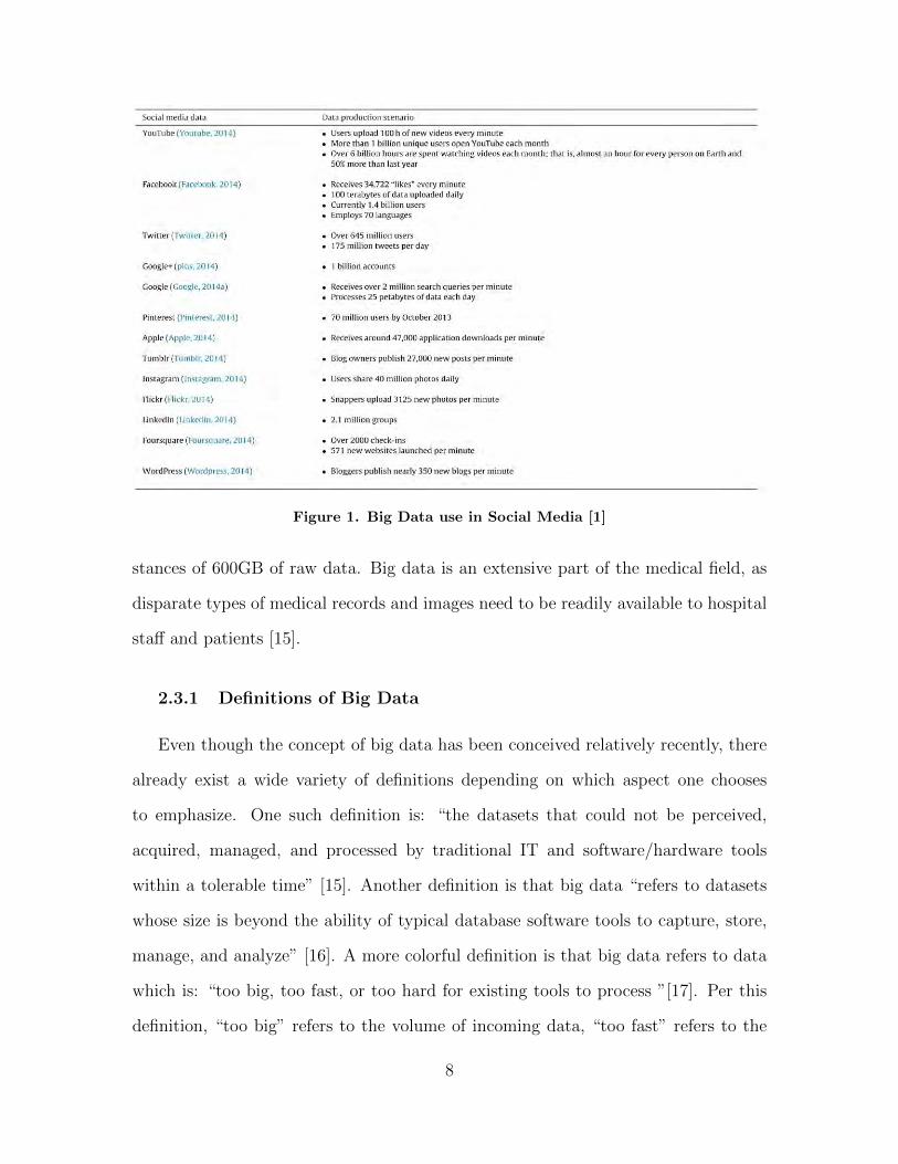
Figure 1. Big Data use in Social Media [1]
stances of 600GB of raw data. Big data is an extensive part of the medical field, as
disparate types of medical records and images need to be readily available to hospital
staff and patients [15].
2.3.1 Definitions of Big Data
Even though the concept of big data has been conceived relatively recently, there
already exist a wide variety of definitions depending on which aspect one chooses
to emphasize. One such definition is: “the datasets that could not be perceived,
acquired, managed, and processed by traditional IT and software/hardware tools
within a tolerable time” [15]. Another definition is that big data “refers to datasets
whose size is beyond the ability of typical database software tools to capture, store,
manage, and analyze” [16]. A more colorful definition is that big data refers to data
which is: “too big, too fast, or too hard for existing tools to process ”[17]. Per this
definition, “too big” refers to the volume of incoming data, “too fast” refers to the
8

processing speed required to adequately digest this data, and too hard refers to any
other challenges not adequately captured by the first two concepts [17].
Authors who provide definitions for big data are deliberately vague, as the capa-
bility of modern technology to handle different sizes of data may change over time.
In some sense, as the available technologies to handle big data improve, so will the
requirements, such that the category described as “big data” will continue to evolve
over time.
2.3.2 Five V Model
The Five V Model [3] [18] [19] (sometimes three or four V’s) was created as part
of an effort to characterize what is meant by big data. The Five V’s refer to Volume,
Variety, Velocity, Veracity, and Value:
• Volume: The size of the data set. How much volume is necessary for data to
be big data is difficult to define, as some older definitions cite 1 Terabyte as
qualifying for big data, while more modern definitions may require Pedabytes
or more. The concept of volume captures not just a static size of required data,
but that the size of the data is ever increasing. [3]
• Variety: The different types of information that industries may want to cap-
ture, which do not necessarily fit well together under traditional paradigms.
Some examples may be: streaming videos, customer click streams, pictures,
audio, comments, transaction histories, etc. [3]
• Velocity The speed at which new data is being accumulated, the speed required
for data streaming, and the speed at which decisions are made. [20]
• Veracity: The inherent uncertainty that exists in data. For instance, social
9
media posts reflect user sentiment and often are not fact based. Even so, col-
lecting this kind of data can be extremely useful for some industries. [21]
• Value: refers to the value of the data itself, which for big data applications
often comes from the high quantity of data and how it can be integrated and
understood. In order words, this data is valuable because of its volume, small
volumes of this kind of data would not have the same value. [21]
Figure 2, created by IBM, provides additional context for the Five V’s with respect
to how they comprise big data.
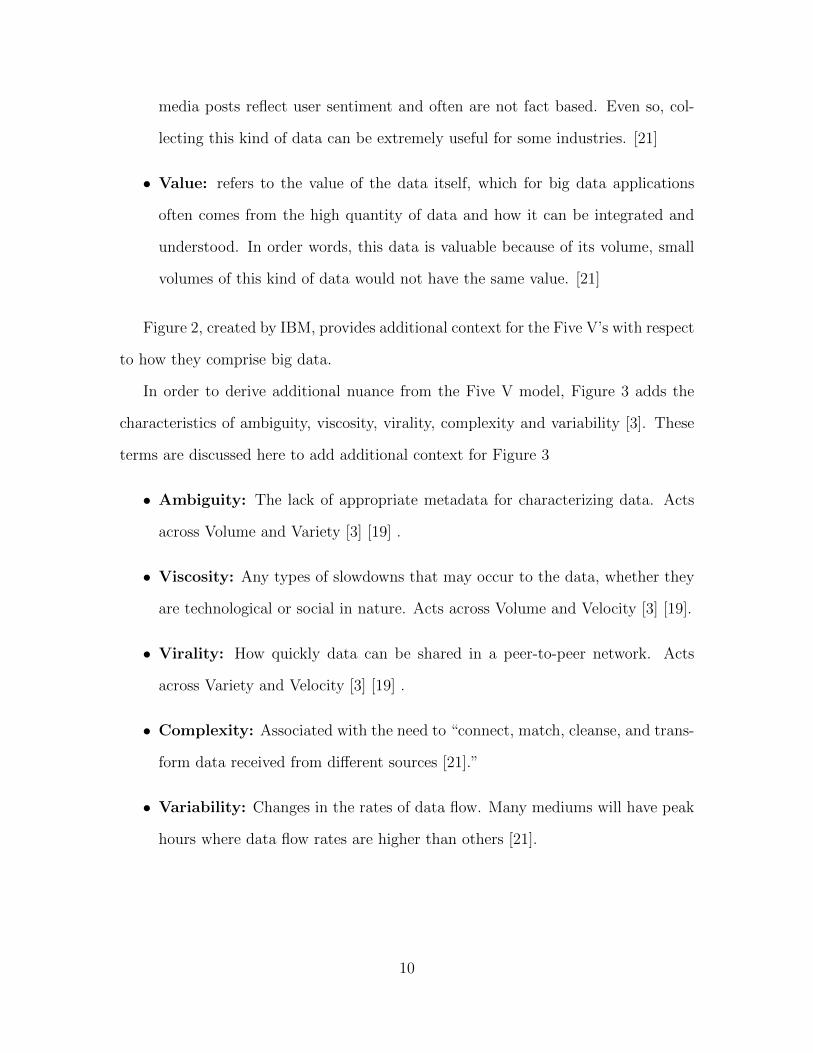
In order to derive additional nuance from the Five V model, Figure 3 adds the
characteristics of ambiguity, viscosity, virality, complexity and variability [3]. These
terms are discussed here to add additional context for Figure 3
• Ambiguity: The lack of appropriate metadata for characterizing data. Acts
across Volume and Variety [3] [19] .
• Viscosity: Any types of slowdowns that may occur to the data, whether they
are technological or social in nature. Acts across Volume and Velocity [3] [19].
• Virality: How quickly data can be shared in a peer-to-peer network. Acts
across Variety and Velocity [3] [19] .
• Complexity: Associated with the need to “connect, match, cleanse, and trans-
form data received from different sources [21].”
• Variability: Changes in the rates of data flow. Many mediums will have peak
hours where data flow rates are higher than others [21].
10

?
Extracting business valuefrom the 4 V’s of big data
The fifth “V”?Big data = theability to achievegreater Valuethrough insightsfrom superioranalytics
Volume
Veracity Variety
Velocity
90%
90%
80%
of today’sdatahas been created in just the last2 years
is the estimatedamount of money thatpoor data quality coststhe US economy per year
of datagrowth is video,images anddocuments
(...enough to fill10 millionBlu-raydiscs)
72 hoursof footage
uploaded to YouTube
216,000Instagram posts
204,000,000emails sent
This includes tweets, photos, customer purchase historiesand customer service calls
is the estimatedrate of global
Internet traffic
by 2018
50,000GB/second
$3.1 trillion of generated datais “unstructured”
Every daywe create
2.5quintillion
bytes of data
1 in 3business leaders don’t trust the information they use to make decisions
Every
60secondsthere are:
Scale of data Speed of data
Certainty of data Diversity of data
Case study: A US-based aircraft engine manufacturer now uses analytics to predict engine events that lead to costly airline disruptions, with 97% accuracy. If thisprediction capability had been available in the previous year, it would have saved $63 million.
IBM, the IBM logo, and ibm.com are trademarks or registered trademarks of International Business Machines Corp., registered in many jurisdictions worldwide. Other product and service names might be trademarks of IBM or other companies. A current list of IBM trademarks is available on the web at “Copyright and trademark information” at www.ibm.com/legal/copytrade.shtml.
Unlock the value of your big data.Start here: ibm.co/technologyplatform
Figure 2. The Four V’s of Big Data [2]11

Figure 3. The Five Vs of Big Data [3]
2.4 Data Modeling
Data Modeling is an aspect of the database design where the relationship between
data of interest is modeled, and the appropriate schema and naming conventions
chosen and applied. When done well, it makes the actual implementation of the
database easier, and aids with updates and changing requirements in the future.
There are generally considered to be at least three stages or layers of data modeling:
The Conceptual Layer, Logical Layer, and Physical Layer [22] [23].
• Conceptual Layer: The highest level of data modeling and describes what
the database contains. This would be typically developed by the business stake-
holders and the database architects. This layer is agnostic with regards to the
12
specific implementation of the database, it will serve to help organize the rele-
vant PNT metadata once collected [22].
• Logical Layer: Goes into additional detail on the specific rules and schemas
that relate the data together, designating how the database should be imple-
mented. It is still above the level of a specific Database Management System
(DBMS) implementation [22].
• Physical Layer: Describes the database with respect to how it will be imple-
mented in a specific DBMS. The relationships between data, types of data, and
names should should be detailed in whatever convention is appropriate for a
specific implementation [22].
One of the key concepts when asking the question of the intended purpose of
relational vs non-relational data bases is that of polyglot persistence. This refers
to understanding the nature of the data which is to be stored, so that that the
appropriate database model and tool can be used. The end result is that even a
single organization may end up using multiple different types of databases base on
their different data storage requirements and the nature of the data to be stored [24].
Programs are well-known to consist of a fusion of algorithms and data structures.
In older relational database models, the algorithms which defined how data was orga-
nized and queried were more sophisticated than the data itself. In modern big data
applications this is reversed. The sheer amount of data requires more sophisticated
data structures organized by simpler algorithms [15]. Still, relational databases offer
powerful capabilities, and efforts are being made to generated databases which offer
the power of relational databases with more modern database models [25].
For most of the history of database development, the relational database model
has been considered to be the standard. As will be discussed in the next section,
13
non-relational databases (sometimes called NoSQL), have risen in prominence in the
2000’s mostly due to problems associated with “big data,” especially as it relates to
Volume, Velocity, and Variety [19].
2.5 Relational Databases
The relational database was created by E.F. Codd in 1970 [26]. It was based on
principles of Mathematical Set Theory and Relational Theory in order to establish
relationships between pieces of information [27]. The primary data structure in the
relational database is the table. Every row of the table contains unique information,
and multiple related tables are linked together by the use of keys [28].
One of the main features of relational databases is that they are Atomicity, Con-
sistency, Isolation, and Durability (ACID) compliant as defined below [27] [29]:
• Atomicity: If a transaction is left unfinished, the entire transaction is consid-
ered to have failed and the database is unaffected.
• Consistency: The database is in a valid state both before and after transac-
tions.
• Isolation: Multiple simultaneous transactions do not impact each other’s out-
come.
• Durability: Once data has been updated, this data will endure even in the
case of an inelegant system failure.
Another key characteristic of relational databases is that they are aggregate-
ignorant in nature [24]. This means that, outside of the relationship between tables
that are created by primary and foreign keys and brought together by joins, data is
distributed between tables and not inherently connected. In general, the appropriate-
ness of aggregates for big data applications is what gave rise to NoSQL applications.
14

Similar to how all elements of engineering design include trade-offs, whether or not
an aggregate based database approach is appropriate is entirely based on the nature
and intended purpose of the data [24].
2.5.1 Normalization
Normalization is one of the main methods used to prepare data to be stored in a
relational database. Normalization is mathematical, and proceeds in discrete steps,
each of which build on each other to produce a progressively more normalized set of
data. Normalization serves to break up data into smaller parts so that useful rela-
tionships between them can be examined, and that they can be managed efficiently.
One goal of normalization is that data duplication is avoided [30].
Normalization comes with benefits and hazards, and for that reason must be bal-
anced based on the intended database application. Some advantages to normalization
are that less physical space is required to store the data, the data is better organized,
and that minute changes can be made to the database. Some disadvantages are that
additional normalization results in additional tables, resulting in larger queries that
are potentially time consuming, and a database that is overall less user friendly [30].
Data normalization progresses according to the following forms. Each form as-
sumes that the data is compliant with the prior forms.
• First Normal Form: Dictates that only a single piece of information is stored
in a given field. The classical example of this is how an address might be broken
into a street, city, and zip code [31].
• Second Normal Form: When data is converted to this form, partial depen-
dencies are removed from from the database tables. In other words, all fields in
table rely on the primary key of that table exclusively [30]. An example might
15

be a table which contains a student, a student id, and class id. The class id
does not depend on a given student, and so should be in its own table.
• Third Normal Form: When data is in third normal form, this means that
a table “is in second normal form AND no non-key fields depend on a field(s)
that is not the primary key. [31]” Another way to say this is that all transitive
dependencies are removed. A potential example of this is if both a student’s
city and country of origin are included in the table. However, if a student is
from a given city, they will always be also from the country in which that city
is located, so a transitive dependency is present and the table is not in Third
Normal Form. The solution involves creating an additional table and separating
out this information, or not including it at all [32].
• Boyce Codd Normal Form: This form, which is sometimes called Normal
Form 3.5, is a slightly stronger version of Third Normal Form. For Boyce Codd
Normal Form, every determinant must be able to be the primary key. In other
words, if any value in a row can be used to determine another value in a row,
that value must be capable of being the primary key of the row [31].
There are additional normal forms beyond those listed here which become increas-
ingly mathematical and complex. They are not necessary to understand the design
laid out in this thesis.
2.5.2 Entity Relationship Diagrams
An Entity Relationship Diagrams (ERD) is a standard way to show the relation-
ships between tables in a relational database [30]. The specific details of how ERDs
are constructed will not be detailed here, as there is abundant available information
online [33] [34] [28], but in general they are simple to understand. ERDs are used in
16
Section 3 and in Appendix A to help describe the database design.
2.5.3 Structured Query Language
SQL is the standard language used to implement relational databases. SQL is
considered to be a declarative language, meaning that a programmer would enter
commands related to the desired result, rather than explicitly telling the program
what to do (in contrast to most programming languages) [35]. As there are a multitude
of free resources available to learn SQL online [36] [37] [38] only the highlights will be
reviewed here. SQL will be one of the main features of this thesis, so as additional
concepts associated with design and testing will be reviewed as they are introduced.
The details of how SQL is used to build out the databases and test queries are available
in Appendixes E and E.
SQL is considered to be composed of four smaller programming languages: [35]
• Data Definition Language (DDL): All SQL commands which define the
structures of the tables, views, and objects along with other data containers
within the database. Commands such as TABLE fall into this category.
• Data Manipulation Language (DML): The commands which insert and
delete data to and from the data structures generated with DDL.
• Transaction Control Language (TCL): The commands which control the
transactions of DDL and DML commands.
• Data Control Language (DCL): The ability to grant or deny access to the
use of DDL and DML commands. This is associated with administrator control
over a database.
17
2.5.4 SQLite
SQLite is a serverless, zero configuration, self-contained Relational Database Man-
agement System (RDBMS) which implements the SQL. It runs directly after down-
loaded, and does not require installation. SQLite is commonly used in portable
devices, such as smart phones and smart TVs, and is a common fixture in portable
applications. SQLite is limited in its size potential, as the entirety of a database is
recorded within a single file on a computer, and is therefore not a good fit for the
entirety of this big data project. Even so, it is a natural fit for prototyping a database,
and iterating quickly through the trial and error process before the database is ready
to store a library of PNT data [35].
2.5.5 PostgreSQL
PostgreSQL is an open source, object-relational database system which dates back
to 1986 at the University of California at Berkely [39]. PostgreSQL offers a variety of
attractive features which make it a strong candidate for developing a PNT database.
This RDBMS supports arrays and documents (such as JSON), along with 160 of the
179 SQL features. Furthermore, PostgreSQL supports table partitioning, which would
allow for a database to be distributed across multiple computers [40]. PostgreSQL is
also extensible, in that additional data types, functions, and operators can be added
[39]. Given this suite of features, PostgreSQL would be a good solution for many big
data problems, depending on their specific requirements [40].
2.6 Non-Relational Databases
Relational databases have been the standard approach to database design since
their inception. However, the relational database model has not traditionally been
a good fit for many modern big data applications, especially in the case where large
18

amounts of unstructured data are necessary. It is in response to this that NoSQL
databases have been designed and popularized [27].
The term NoSQL refers to the set of database options which do not use the re-
lational model (with SQL as its most common implementation language), as their
primary approach. NoSQL, and the related requirements which lead to the incep-
tion of its various implementations, warrant additional paradigms to help understand
its role in database design. The CAP theorem will be discussed in order to help
understand some of the limitations facing databases when applied to big data [41].
Following this, the Basically Available, Soft state, Eventual consistency (BASE) prop-
erties of NoSQL will be reviewed in order to help understand how NoSQL deals with
the shortcomings of not utilizing the relational model. Finally, the four standard
categories of NoSQL will be reviewed.
2.6.1 The Consistent, Available, or Partition Tolerant Theorem
The CAP theorem was theorized by Eric Brewer in 2000 based on his work at
the University of California, Berkley [42]. This theorem applies to distributed data
systems, and theorizes such systems are fundamentally limited. Figure 4 provides a
visual depiction of the CAP theorem, along with how it relates to various common
database programs. In effect, only two of the following three traits is available for a
distributed database [43].
The explanation of the CAP theorem is as follows: [43] [44]
• Consistent: Writes are atomic and that once an update takes place, that
update is immediately available to all users of the database.
• Availability: The database will always return a value as long as at least one
server is running.
19

Figure 4. The CAP theorem visualized [4]
• Partition Tolerant: The database will continue to function even if server
connection is lost (amongst host computers). It is implied that if a server is
partition tolerant, then it is not distributed.
Determining which of these traits should be compromised is based on the specific
design application. In general, PostgreSQL, which is the database design approach of
choice for this project, is considered to be Consistent and Available but not Partition
Tolerant [43]. In comparison, MongoDB, which was the potential NoSQL solution of
choice, is considered to be Consistent and Partition Tolerant but not always available
[43]. Based on design choices, PostgreSQL is capable of utilizing partitions, whether
by Master/Slave configurations across multiple computers [43] or by separating out
rows between schema in a single database [39].
20

The PNT database design laid out in this thesis recommends a distributed solu-
tion, as the database will grow prohibitively large to be contained on a single com-
puter. Also, ultimate usage of the database will likely discriminate between very large
files such as images and the type of data that would be stored in rows. There will be
rows which contain pointers, called Object Identifier (OID)(s), which lead to other
large files, potentially on other computers. Under such a distributed design approach,
the database would be Partition Tolerant, but may not be Consistent or Available
in every case depending on implementation. For the purposes of this project, every
database tested is not partitioned, as all testing took place on a single test computer.
2.6.2 Basically Available, Soft state, Eventual consistency Properties
The BASE properties are considered to be an alternative to ACID and are essen-
tially an extension of the CAP theorem, noting that these properties are continuous
and not discrete [45]. It is sometimes said that NoSQL databases have the BASE
properties in lieu of SQL’s ACID, meaning that they are Partition Tolerant and
Available but not Consistent [41] [24]. The elements of BASE are as follows: [46]
• Basically Available: Data is mostly available, but due to updates internal
to the database it may take time in some cases to get at the data, or at other
times the request might fail altogether.
• Soft State: The database is consistently updating over time, so that even when
it is not being utilized updates may be occurring.
• Eventual Consistency: Consistency is not guaranteed after every transaction,
but over time the system will return to consistency.
21
2.6.3 Standard Types of Not only SQL Databases
As discussed before, the defining characteristic of NoSQL is that it is not SQL,
or not based exclusively on the relational model. To understand the use cases and
potential benefits of NoSQL, it is prudent to discuss its main categories and their key
characteristics.
2.6.3.1 Key-Value Databases
Key-Value databases are the simplest type of NoSQL database. They are es-
sentially hash tables that only have two values, the primary key and the file that’s
associated with it [41]. Key-Value databases do not care what that file is, it could
be a Binary Large OBject (BLOB) containing any kind of information. It is the
responsible of the application to understand how to utilize this information. One
possible application is a shopping cart on a popular website. The primary key might
be associated with a specific user, and the contents of their shopping cart would be
what they have selected to potentially buy. This system is very fast, but also very
simple, and does not allow for the sophisticated queries available to RDBMS [24].
SimpleDB, which was created by Amazon, is an example of a key-value databse [47].
2.6.3.2 Document Databases
Document databases utilize documents of various types, with JSON being one of
the more common formats. Unlike the RDBMS model, these documents can contain
different information from each other, even if they have some common elements [41].
Depending on the application, these documents may have no structure at all. The
document database collection could be considered analogous to a RDBMS table, and
individual documents could be considered similar to rows [48]. Document databases
often use master/slave setups along with replica sets to increase data availability. In
22

this setup, duplicate nodes vote amongst themselves based on design parameters to
decide which is the master and slaves, and in the case of a master going offline a slave is
elevated to master. The master accepts all transactions and sends them to the slaves,
all to increase availability. Unlike the key-value database, the document database
does allow for queries to interact with the contents of the documents. MongoDB
in particular has its own language which is similar to SQL. Due to the flexibility
of the schema, queries may be difficult if there are substantial differences between
documents [24].
2.6.3.3 Column Family Stores
The general idea of a column family store is that columns are the primary data
structure feature, as opposed to rows. In a column family store, all of the relevant
information will be stored within a column, along with an associated id for each
piece of information which correlates to ids located in other columns, along with a
time stamp. A column family is a set of associated columns, which could almost
be thought of as a table in a RDBMS. One critical difference is that the rows do
not have to have the same columns, or this could be thought of not all columns
applying to every row. In comparison to RDBMS, column family stores do not have
as sophisticated of a query system. They are also not good for integrating data
using mathematical operators [24]. Cassandra, which was created by Facebook, is an
example of a column-oriented database [47].
2.6.3.4 Graph Databases
Graph databases use nodes and the links between the nodes to structure data. The
nodes can be thought of as objects, as the links between them define their relationships
to each other. The schema is flexible, so that the relationship, “likes,” could be used
23
to link a person object to a food object. Note that these links are one-way, so the
person would like the food, but not the other way around. The flexibility of these
schema make adding relationships easier in graph databases than in RDBMS. Query
systems such as Gremlin are available to perform queries on graph based databases
[24].
2.7 Data Warehouses, OLTPs and OLAPs
A data warehouse has been defined as “a subject-oriented, integrated, time-
varying, non-volatile collection of data that is used primarily in organizational de-
cision making [49].” The data warehouse supports the functions of OLAP. When
designing a data warehouse for a big data solution, the data volume, variety, and
velocity, and ambiguity all need to be understood [19]. Typically, data stored in a
data warehouse is considered to be heterogeneous and derived from multiple sources
[50]. Data warehouses are used in conjunction with OLAPs for data analysis.
OLAPs are online tools which are used by businesses for data analysis, and serve
to integrate data from multiple databases to inform business decisions. OLAPs typi-
cally have a low number of users in comparison to OLTPs [51], and do not typically
result in updates to these databases. Typical analytical services provided by OLAPs
are planning, budgeting, forecasting, and analysis. A potential example of a OLAP
system is comparing the number of phone sales between separate months at one loca-
tion, and to the phone sales of another location where that data is stored in a separate
database [52].
OLTP services, in contrast, typically have many more users per day. OLTPs are
ACID compliant and are used to process data, in contrast to analyzing data [52].
OLTPs are typically used for short, repetitive, clerical work that is atomic in nature
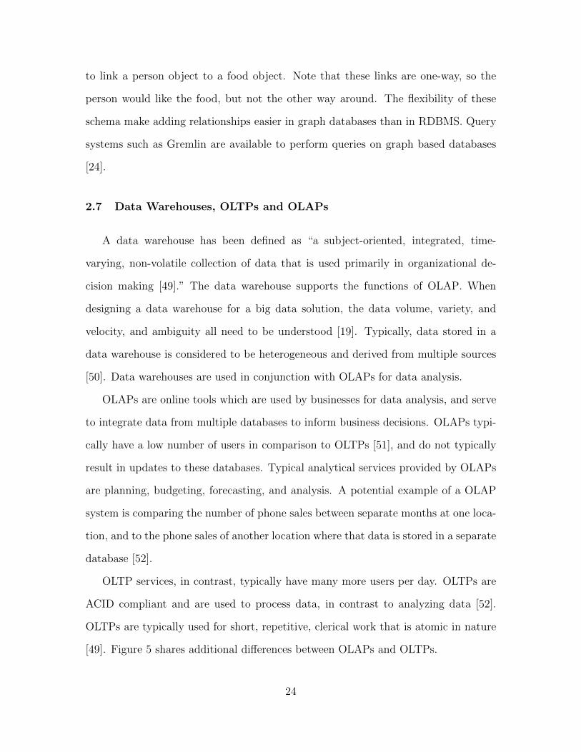
[49]. Figure 5 shares additional differences between OLAPs and OLTPs.
24
Figure 5. OLAP vs OLTP [5]
The database in this thesis in general can be thought of as a data warehouse with
an OLAP application. Researchers will use this data to perform analysis and to select
data sets which are of interest to their research. This is not a perfect fit, as SDM
data is normalized, in contrast to the general view of OLAP. Also, even though this
database will be distributed, it is still a single database.
2.8 NewSQL
NewSQL has been defined as “a class of modern relational DBMSs that seek to
provide the same scalable performance of NoSQL for OLTP read-write workloads
while still maintaining ACID guarantees for transactions [53].” Rather than retrofit
existing SQL DBMSs for scalability, which they were not originally designed for, many
NewSQL DBMSs are designed from the bottom up with scalability and cloud com-
puting in mind from the beginning. NewSQL tend to focus more on the Consistency
25

and Partition Tolerant elements of the CAP theorem over Availability [51]. Some
have also referred to NewSQL as “ScalableSQL,” while acknowledging that “the new
thing about the NewSQL vendors is the vendor, not the SQL [54] .”
Citus is one possible open source NewSQL product which extends PostgreSQL
rather than designing a new product from the ground up [51]. Citus acts by dividing
tables horizontally across multiple nodes, so that they appear as separate tables to
an actual user. This allows for horizontal scaling, which is not typically associated
with SQL databases [51]. However this does not fit a strict definition of NewSQL
as defined by Pavlo and Aslett (2016) which requires that they not be built on the
infrastructure of existing SQL systems [53].
As NewSQL is essentially a way to apply the scalability of NoSQL to OLTP
systems, further review is not necessary to help understand the underlying design
decisions of presented in this thesis.
2.9 Multi-Objective Database Queries
MO database queries are queries where the result set balances multiple user-
objectives. MO Retrieval can be defined as a database containing N objects, n char-
acteristics which describe the objects, and m monotonic functions which score the N
objects based on the n characteristics [55]. The goal is to score and return the objects
based on the their collective scores from all the m monotonic functions.
One major categories of MO database queries is the top k query, which is where
users set preferences for query returns. These preferences are not requirements, and
a result set will still be returned in the case that not all preferences are met. The
objects in the database are scored according to these preferences and returned to the
user [55], and only the top k are returned, where k is an arbitrary number defined to
reduce the size of the result set [56] A straight forward example would be a real-estate
26
database which contains information on a set of houses for sale. A user searching a
real-estate database would set the preference for a number of bedrooms and a certain
price range. Even if no houses meet these specific requests, the houses which best fit
this preference would still be returned [57].
An additional major category of MO database queries is the skyline query. Sky-
line queries return the result set of objects, which, given a dominance relationship,
cannot be dominated [58]. Given a data set of multidimensional objects, an object is
considered to dominate another object if it is equal in all respects, and better in at
least one respect [58].
The available literature offers a variety of algorithms to perform these queries and
their variants [59] [60] [55] [56] [57] [58]. While not used to help discriminate between
possible database designs, these algorithms are available to aid in the construction of
more advanced queries once the final database is operational.
2.10 Cloud Computing
Cloud computing represents the availability of resources over what is called a
cloud, which is information or capability that is available online and can be utilized
remotely. A definition provided by the National Institute of Standards and Technol-
ogy (NIST) Cloud Research Team is that “Cloud Computing is a model for enabling
convenient, on-demand network access to a shared pool of configurable computing
resources (e.g., networks, servers, storage, applications, and services) that can be
rapidly provisioned and released with minimal management effort or service provider
interaction [61].”
There are three essential cloud service models which are highlighted in Figure 6:
Cloud Software as a Service (SaaS), Cloud Platform as a Service (PaaS), and Cloud
Infrastructure as a Service (IaaS). A description of each is provided below [6] [61]
27

[62].
• SaaS: A web-based application which gives access to vendor provided software
over a network. Facebook, Gmail, and others are examples. It is not necessary
that the providers software be download in this model.
• PaaS: A cloud base for developing and testing different applications. PaaS
provides a location for user created software to be deployed to the cloud.
• IaaS Computing resources which are provided over a cloud. IaaS provides an
infrastructure over which customers can design and utilize applications. This
infrastructure may include storage, servers, networking hardware, etc.
Many big data applications utilize some kind of cloud service to make themselves
available to their customers [61] [6]. The PNT database operational solution will need
to be deployed in some kind of a cloud service to be useful to researchers. Of the
service models discussed above, SaaS is the best fit, as the database will be accessed
online, where researchers will perform queries with a user interface, which will then
access the database and return the solutions to the users.
2.11 Relevant Research
Following a full literature review, the relevant research on big data as it relates to
PNT data is sparse. Most sources discuss traditional vs modern big data paradigms,
how big data is applicable to major fields such bio-medical and social engineering,
and its benefit to the medical community (amongst other topics) [63] [64] [13] [65]
[25] [48].
One particular area of interest is the Resonant Girder service. Girder is a system
designed for large data and analytics management and is implemented in MongoDB
28

Figure 6. Cloud Computing Services [6]
and is available over Amazon Web Services. Girder works with blobs and their meta-
data, and is very versatile, providing data indexing, provenance and abstraction.
Girder is not a general purpose database, and is not designed to handle tabular data
[66]. While interesting, it is not a good fit for this project, due to the tabular nature
of the SDM.
2.12 Summary
This literature review covered a variety of topics with respect to database design,
especially as it relates to the concept of big data. The topics of data modeling were
discussed, along with the concept of the Five V’s and its variations. It is envisioned
that the data to be recorded in this database will be relatively low on Variety and
Velocity, but relatively high in Volume. This is owing to the expectation that AFIT
29
will host a limited number of test flights per year, but that the test flights will be in
the SDM format and in some cases can be millions of LCM events per flight. This
indicates that use of the database will be relatively frequent, potentially being queried
dozens of times, that the database will be updated only a few times per year, and
that each update will add millions of rows.
Following this, Relational Databases, NoSQL, and NewSQL, along with OLTP,
OLAP, and data warehousing were all reviewed. These topics are related, and in many
cases were designed in to solve different types of problems related to the changing
nature of data over time. Given that the SDM format is standardized and tabular
in nature, it is reasonable to expect that a RDBMS utilizing SQL is a good choice
as a solution. Specifically, PostgreSQL offers a suite of useful capabilities, and is
capable of being distributed across multiple database. The qualities of Consistency
and Partition Tolerance of the CAP theorem will likely be emphasized, but this does
not mean that the database will frequently be unavailable. Due to updates being
relatively infrequent once the database is fully operational, the database manager
can schedule downtime when uploading new data so that the cost to availability is
limited. The service that the database provides falls more into the category of OLAP
than OLTP, due to the primary use case being data analysis and the expectation that
mundane users will not be performing transaction updates against the database. The
specific management details for this database are beyond the scope of this thesis.
Next, the concept of MO database queries was introduced. This is intended to lay
the groundwork for understanding more advanced queries that can be used against
the database designed in this thesis. In Section 4, a paper proposing the combination
of the KP and the SCP as a multi-objective NP-Hard database query is presented.
The proposed algorithms do not incorporate sky-lining or top-k queries, but it would
be possible to utilizing these as researchers utilize the database and more realistic use
30

cases emerge.
Finally, the literature review covered the concept of cloud computing. It is envi-
sioned that the database will be made available on a cloud so that it can be accessed
remotely by researchers. This will most likely be a SaaS, as researchers would be
interested in directly accessing the user interface for the database in order to per-
form queries. The development of this user interface and its subsequent deployment
to a cloud service is beyond the scope of this thesis, but it will be one of the first
implementation details to consider once a database schema is chosen.
31
III. Design
3.1 ION/PLANS Paper Introduction
Section 3 of this thesis summarizes the design decisions and test results of the
database. Sections 3.1-3.6 are composed of a paper submitted to the Institute of
Electrical and Electronics Engineers (IEEE) Institute of Navigation (ION)/Position
Location and Navigation Symposium (PLANS) Conference scheduled for April 23rd to
April 27th. Sections 3.7-3.9 are composed of material removed from the ION/PLANS
paper due to space restrictions. Section 3.7 discusses details of how the test databases
are generated. Section 3.8 presents indexes that are used to speed up queries against
the SDM data type tables, and Section 3.9 presents three figures for the Metadata
Query Test that are summarized in Section 3.5.2.1.
Performing flight tests is a common part of researching complementary PNT sen-
sors and filters for sensor integration. These tests allow for different arrangements of
sensors to be tested, along with their integrating software frameworks. Unfortunately,
tests cost time and money, and require planning for necessary resources to be avail-
able. It would be helpful for researchers if this collected data were readily accessible,
in order to facilitate filter research without needing to run redundant tests.
As an example, the AFIT has approximately one-hundred navigation data logs
(missions) available to help facilitate research. If these data logs were collected into a
database with a standard format, it would provide a common location for researchers
to look for helpful data, and to place new collected data. Other organizations in
the navigation community may also benefit from adapting the database design to
their data sets. The design will allow for testers to record observations from the day
of testing in standardized formats, store details of sensor and vehicle arrangements,
and record data necessary to model the test sensors at a later time. Testing three
32
different database schema against queries of interest will demonstrate that the schema
are useful, and testing them with 1000 log files containing hundreds of million of rows
of navigation data will demonstrate that the schema scale.
We propose a standard schema for sensor and metadata schema for navigation
flight tests and three different designs that organize this data in relational databases.
These schemas allow researchers to distinguish between logs based on the types of data
stored, the sensors and configurations used to record this data, the type of vehicle(s)
affiliated with the data set, the environments that the vehicle(s) operated in, and more
nuanced elements based on the specific recordings of the data itself. These databases
are able to store the sensor data, metadata about the sensors, and affiliated metadata
of interest. This paper details the schema for these database approaches, the queries
and test scripts used to test these approaches, along with testing results and analysis.
The test results are expected, and are explained based on the database structure and
how it relates to the queries used. The paper recommends the best overall performing
database design in Sections 3.5 and 3.6.
3.2 Relevant Background
This paper specifically concerns the design of a database to store PNT data, along
with necessary metadata, using the SDM as the sensor data baseline. Due to AFIT’s
available data logs originally having been recorded as LCM messages, LCM is used
as a database data storage format. These logs can be thought of as a series of LCM
events which contain SDM data. Additional information on the LCM event format
is available here [11] [67]. It is anticipated that SDM messages could be transmitted
in additional standards.
SDM is defined in YAML, a human-readable markup language. To design a
database for this data, it is not necessary to understand the data in detail from
33
a navigation perspective, except that the database needs to be optimized for the
types of queries that a member of this field is interested in. Members of the ANT
center at AFIT provided the basis for the queries outlined in this paper.
The remainder of Section 3.2 will discuss the background of two major database
categories, and present justification for which category was chosen for this project.
Section 3.3 will present design requirements and approaches, Section 3.4 will present
the design of experiments, Section 3.5 will present the testing results and analysis,
and Section 3.6 will summarize this paper and discuss future work.
3.2.1 PNT Database Characteristics
The database characteristics are presented here to keep the high level database
background in context, and to help other organizations tailor their database imple-
mentations based on their specific use case.
1. The database will be updated when flight tests occur (infrequent writes).
2. The database will be used daily (frequent reads).
3. The sensor data will be in the SDM 2.0 format.
4. Sensor data will be wrapped in LCM events.
5. Every update to the database will include over one-million sensor measurements,
and assorted sensor metadata.
6. The database will be updated with approximately one-hundred sensor data logs
after it is first launched. These will be converted from legacy sensor formats
and may have incomplete metadata.
7. The database will be a distributed system when it is first launched.
34

8. The database will be available over a cloud service.
The database designs presented in this paper do not address numbers 7 or 8 in
the list above. These two characteristics will be addressed when choosing a database
program to ensure that they are supported to enable future work.
3.2.2 Relational Databases
The relational database was created by E.F. Codd in 1970 [26]. It was based on
principles of Mathematical Set Theory and Relational Theory to establish relation-
ships between pieces of information [27]. The primary data structure in the relational
database is the table. Every row of the table contains unique information, and mul-
tiple related tables are linked together by the use of keys [28]. Relational databases
are commonly associated with SQL.
A main feature of relational databases is that they are ACID-compliant, defined
as guaranteeing: [27] [29].
• Atomicity: If a transaction is left unfinished, the entire transaction is consid-
ered to have failed and the database is unaffected.
• Consistency: The database is in a valid state both before and after transac-
tions.
• Isolation: Multiple simultaneous transactions do not impact each other’s out-
come.
• Durability: Once data has been updated, this data will endure even in the
case of an inelegant system failure.
Another key characteristic of relational databases is that they are aggregate-
ignorant in nature [24]. This means that, outside of the relationship between tables
35

that are created by primary and foreign keys and brought together by joins, data is
distributed between tables and not inherently connected. In general, the appropri-
ateness of aggregates for database applications is what gave rise to NoSQL. Whether
an aggregate based database approach is appropriate is entirely based on the nature
and intended purpose of the data [24].
3.2.2.1 SQL
SQL is the standard language used to implement relational databases. SQL is
considered to be a declarative language, meaning that a programmer would enter
commands related to the desired result, rather than explicitly telling the program
what to do (in contrast to most programming languages) [35]. SQL will be one of the
main features of this research, so as additional concepts associated with design and
testing will be reviewed as they are introduced.
SQL is composed of four smaller programming languages: [35]
• DDL: SQL commands which define the structures of the tables, views, and
objects along with other data containers within the database.
• DML: The commands which insert and delete data to and from the data struc-
tures generated with DDL.
• TCL: The commands which control the transactions of DDL and DML com-
mands.
• DCL: The ability to grant or deny access to the use of DDL and DML com-
mands. This is associated with administrator control over a database.
36
3.2.2.2 PostgreSQL
PostgreSQL is an open source, object-relational database system which dates back
to 1986 at the University of California at Berkely. PostgreSQL offers a variety of
attractive features which make it a strong candidate for developing a PNT database.
This RDBMS supports arrays and documents (such as JSON), along with 160 of
the 179 SQL features. Furthermore, PostgreSQL supports table partitioning, which
allows for a database to be distributed across multiple computers. [40] Given this
suite of features, PostgreSQL would be a good solution for many big data problems,
depending on their specific requirements [40].
3.2.3 Non-Relational Databases
Relational databases have been the standard approach to database design since
their inception. However, the relational database model has not traditionally been a
good fit for many modern applications, especially in the case where large amounts of
unstructured data are necessary. It is in response to this that NoSQL databases have
been designed and popularized [27]. The term NoSQL refers to the set of database
options which do not use the relational model (with SQL as its most common imple-
mentation language), as their primary approach.
3.2.3.1 The CAP Theorem
The CAP theorem was presented by Eric Brewer in 2000 based on his work at the
University of California, Berkley [42]. This theorem applies to distributed data sys-
tems, and postulates that such systems are fundamentally limited. The explanation
of the CAP theorem is as follows: [43]
• Consistent: Writes are atomic and that once an update takes place, that
update is immediately available to all users of the database.
37

• Available: The database will always return a value as long as at least one
server is running.
• Partition Tolerant: The database will continue to function even if the network
connections among nodes of the distributed data system are interrupted. It is
implied that if a server is partition tolerant, then it is not distributed.
There are four major categories of NoSQL: Key-Value Databases, Document
Databases, Column Family Stores, and Graph Databases. As MongoDB, which is
a Document Database, is the primary NoSQL program considered for this project,
Document Databases will be discussed in detail here.
3.2.3.2 Document Databases
The collection is one of the main features of Document Databases. They could
be considered analogous to a RDBMS table, and individual documents could be
considered similar to rows [48]. Unlike the RDBMS model, these documents are not
required to conform to a consistent tabular structure, even if they have some common
elements [41]. Depending on the application, these documents may have no structure
at all. Document databases often use master/slave setups along with replica sets to
increase data available. In this setup, duplicate nodes vote amongst themselves based
on design parameters to decide which is the master and slaves, and in the case of a
master going offline a slave is elevated to master. The master accepts all transactions
and sends them to the slaves, the document database allows for queries to interact
with the contents of the documents. MongoDB in particular has its own language
which is similar to SQL. Due to the flexibility of the schema, queries may be difficult
if there are substantial differences between documents [24].
38

3.2.4 Database Decision Summary
The author chose between PostgreSQL and MongoDB as the possible SQL and
NoSQL solutions for this database. Both programs are free and open-source, and are
well-known database programs. The database designed in this paper is intended to
store standardized sensor data, which is why a relational database was chosen as a
candidate for a solution. The available sets of sensor data are stored in LCM log files,
and could be stored as documents in a document NoSQL database.
We considered the CAP theorem when choosing between PostgreSQL and Man-
goDB. Despite PostgreSQL being typically characterized as being Consistent and
Partition Tolerant, it is capable of utilizing partitions, whether by Master/Slave con-
figurations across multiple computers [43] or by separating out rows between schema
in a single database [39]. MongoDB is designed to function as a distributed database
[43]. Therefore, both MongoDB and PostgreSQL can be Consistent and Partition
Tolerant at all times, and Available except during database updates. They are both
acceptable for this database solution under the terms of the CAP theorem.
Both PostgreSQL [68] and MongoDB [69] are supported by Amazon Web Service,
and are therefore acceptable as a database solution in terms of cloud service support.
Comparative query speed is the final factor when comparing MongoDB and Post-
greSQL. Typically, MongoDB performed better when data was unstructured, and
PostgreSQL performed better when data was structured [70]. PostgreSQL was also
found to be almost four times as fast in query speed compared to MongoDB in both
single node and distributed systems with respect to standardized data [71]. When
considering the storage of sensor data, PostgreSQL outperformed MongoDB when
query flexibility was necessary and read performance was prioritized [72].
Based on the superior performance of PostgreSQL when data is standardized,
PostgreSQL is chosen as the database program of choice for this project.
39

3.3 Database Designs
3.3.1 Requirements and Approaches
The following is a list of database requirements developed to serve as the founda-
tion for initial PNT database design decisions.
• Database metadata must be easily queried for ease of analysis.
• Database queries must be optimized for speed.
• Database log files must be available for download from the database.
For this paper, three distinct approaches are implemented and tested. They are
referred to as Approach 1, Approach 2, and Approach 3. The only difference between
them is how they store data collected by sensors. Here is a brief description of each
approach:
• Approach 1: One table is created for each SDM data type. When a log is
added to the database, sensor data is deserialized and added directly to the
corresponding SDM table to create symantically equivalent rows. Row ids are
used to record the original order of the sensor data. Indexes are used to optimize
reads of these tables.
• Approach 2: A new table is created for each SDM data type and each data
log. When a log is added to the database, new tables will be created for each
data type present in the new log. Indexes are not necessary, because the rows
with the lowest and highest ids in each SDM table will be the first and last rows
for that table and that mission.
• Approach 3: The same as Approach 1, with the exception that tables are
not included for the IMU (Inertial Measurement Unit) and OpticalCameraImage
40

SDM data types (described in Table 7. The original data log is also included
in the database to be available for download. In the case that queries need
to look at the IMU or OpticalCameraImage data, the original log file will be
downloaded and parsed using Java. In order to create the original files when
necessary, this approach includes a pointer which links to the original data file
[73].
3.3.2 Table and Relationship Descriptions
Each approach has identical relationships for the sensor Metadata and non-sensor
Metadata sections. The database schema that is common to the three approaches
will be discussed first, followed by the schema which is different.
Figure 7 gives a high level of view of how elements in the database are related.
This figure is presented as an ERD, a standard way to show the relationships between
tables in a relational database [30]. Each box represents either a single table, or a set
of tables which share the relationships shown. All three approaches compared in this
paper share this database overview.
As this is a relational database, each table will be related through foreign keys
which hold pointers to primary keys, and each column will have a specific data type.
Each element will be explored in greater detail in subsequent sections, and a complete
schema is available [67].
3.3.2.1 missionDescription
The missionDescription table is the hierarchical starting point of the database.
Each primary key in the missionDescription table describes a data log which was
uploaded into the database. The columns shown in Table 2 are designed to offer
useful high level metadata to distinguish between data logs.
41
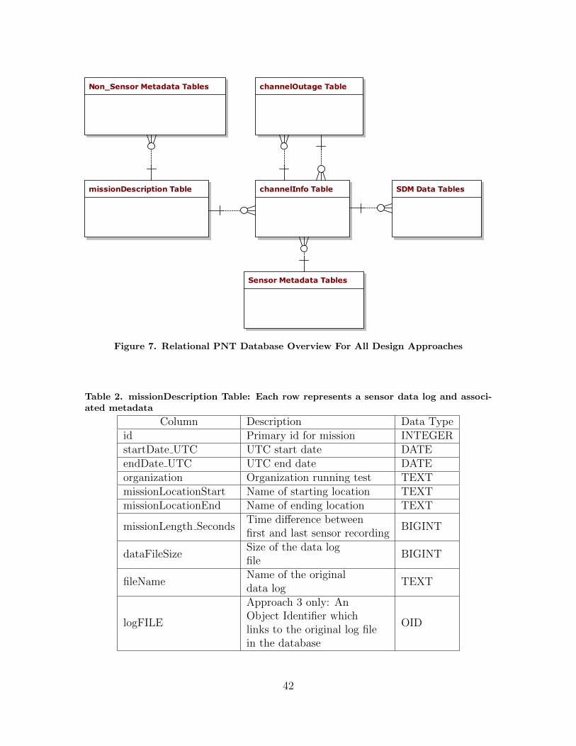
missionDescription Table
Non_Sensor Metadata Tables
channelInfo Table
Sensor Metadata Tables
SDM Data Tables
channelOutage Table
Figure 7. Relational PNT Database Overview For All Design Approaches
Table 2. missionDescription Table: Each row represents a sensor data log and associ-ated metadata
Column Description Data Typeid Primary id for mission INTEGERstartDate UTC UTC start date DATEendDate UTC UTC end date DATEorganization Organization running test TEXTmissionLocationStart Name of starting location TEXTmissionLocationEnd Name of ending location TEXT
missionLength SecondsTime difference betweenfirst and last sensor recording
BIGINT
dataFileSizeSize of the data logfile
BIGINT
fileNameName of the originaldata log
TEXT
logFILE
Approach 3 only: AnObject Identifier whichlinks to the original log filein the database
OID
42
3.3.2.2 Non-Sensor Metadata
The non-sensor metadata tables refer to data that was not generated by sensors
nor is associated with sensors. These tables do not change based on the design
approach.
3.3.2.3 channelInfo Table
The channelInfo table, shown in Table 4 holds the data for all of the channels
which were used on every mission. A channel is the measured data for a specific
sensor and for a specific mission. A given mission will have one or more channels.
Each channel will only ever be associated with a single mission. Each channel has
a foreign key to the sensorInstallationInfo table, which describes a given sensor
and its related sensor metadata.
3.3.2.4 Sensor Metadata
The sensor metadata section of the database design is focused on the sensorInstallationInfo
table described in Table 5. The sensorInstallationInfo table acts as a map to the
other sensor tables of interest. Depending on the use case, especially when converting
older data sets into this schema, not all sensor information may be known. In other
words, it may be known that an IMU sensor was affiliated with a channel, but the
sensor model and more specific intrinsic information may be unknown.
Table 6 shows the other tables associated with the sensorInstallation table
that are not explicitly shown in Figure ??. These provide additional information
about the sensors and vehicles associated with each channel. They are not fully
comprehensive for all possible sensors or vehicles, but do demonstrate the potential
relationships between intrinsic sensor and vehicle data and their associated missions
and data collects.
43

Table 3. Non Sensor Metadata Tables: These Tables record data that helps distinguishbetween data logs but is not directly associated with the sensors
Table Description Data Stored
precipitationType of precipitationand intensity
precipitationintensity
obscuration camera obscuration obscuration
terrainLand environment(s)where test was performed
terrain
skyCoverHow muchsky is exposed
skyCover
maneuversManeuvers performedduring flight
maneuver
loopClosuresLocations and timeswhere an aircraft crossedits own path
timelatitudelongitude
wayPointsWayPoints designatedas part of thetest planning process
timelatitudelongitude
altitudeSegmentsRecorded segments ofincreasing, decreasing,or unchanging altitude
start altitudeend altitudeapproximate duration
unexpectedResultsAny recorded occurrenceduring testing
unexpectedResults
Table 4. channelInfo Table: Connects a data log with its SDM data, and with sensormetadata
Column Description Data Typeid Primary id for channel INTEGER
channelNameName given channel bytesters in data log
TEXT
channelUseChannel’s intended useprovided by testers
TEXT
truthDesignates if the channelrecorded truth data
BOOLEAN
missionDescription idFOREIGN KEY tomissionDescription Table
INTEGER
sensorInstallation idFOREIGN KEY tosensorInfo Table
INTEGER
44

Table 5. sensorMetaData Tables: describes the sensors used to collect data on specificchannels
Table Description Data Stored
sensorInstallationInfoHolds foreign keys to allsensor metadata
Foreign Keys
sensorModelDescribes sensor Modeland Type associated withchannel.
idmakemanufacturertype
vehicleDescribes which vehicleis associated with whichchannel
vehicle
extrinsicSensor-Configuration
Describes theextrinsic valuesto characterizea sensor configuration
leverArmorientationXorientationYorientationZ
sensorSpecificData to identify aspecific sensor
sensorUID
3.3.2.5 Outage Table
The outage table has a many-to-many relationship with the channelInfo table.
This means that an outage may have occurred across multiple channels, and a given
channel may have multiple outages. More details on this table are available [67].
3.3.2.6 SDM Data
The SDM data type is a standardized way to store PNT data. In the six log files
used to test the three database designs, there were eleven distinct SDM data types.
Each of these data types are highlighted in Table 7 along with their description. A
more detailed description of SDM is beyond the scope of this paper, but is available
for review [7] [74]. How this SDM data is stored is the only difference between the
database approaches.
45

Table 6. Other sensorInstallation Tables: These tables record additional sensor infor-mation.
Table Data Stored
aircraftaircraftTypetailNumber
groundVehiclemakemodelyear
GPS Intrinsicgps antenna makegps antenna modelsensorSpecific id
externalAidingClockmakemodelGPS Intrinsic id
system signals trackedsystemTrackedsignalTrackedGPS Inrinsic id
supportedAugmentationSystems supportedAugmentationSystem
IMU Intrinsic
timeCorrelated accelBiasSigmatimeCorrelated accelBiasTautimeCorrelated gyroBiasSigmatimeCorrelated gyroBiasTauvelocityRandomWalkangularRandomWalkaccelerometerScaleFactorUncertaintygyroScaleFactorUncertainty
clock Intrinsic
h0h1h2x0Arrayp0Array
camerafocalLengthcameraImageCenterlensDistortion
46

Table 7. SDM Data Types: Describes the standardized types of sensor data recordedin each data log
SDM Data Types Description
imu
Inertial Measurement Unit (IMU) deltavelocity and delta rotation measurementsfrom the device’s three axis accelerometersand three axis gyroscopes.
velocity3d 3-dimensional velocityvelocity1d 1-dimensional velocityspeed Speed as the magnitude of the velocity vectoraltitude Height above a specific world framegeodeticposition3d 3D WGS-84 GeodeticPosition
threeaxismagnetometerMeasures magnetic field as a 3-dimensionalvector
positionvelocityattitudeIncludes position, velocity, and rotation,and uncertainty
opticalcameraimage Image from an optical cameragnss Raw measurements from a GNSS receivergpsephemeris Ephemeris describing GPS satellite locations.sensorRegistrationAck Message to register sensornon SDM Message LCM message is not an SDM data type
47

3.4 Design of Experiments
Table 8 describes the test equipment. The databases are stored on the Solid
State Drive (SSD), while the test scripts are run within the Integrated Development
Environment (IDE) which is installed on the laptop hard drive.
3.4.1 Database Population
We used six databases to test the three approaches. Each approach was built once
with 100 data logs, and once with 1000 data logs. These databases are constructed
from six files containing SDM data in the LCM format, which are repeatedly loaded
into the databases using the schema described in Section 3.3. The databases are also
updated with randomized sensor metadata and non-sensor metadata. We expect that
this may cause some variation between how the six data bases perform with respect to
the metadata queries. This is acceptable, because the three approaches have identical
schemas for how this data is stored, and will not be distinguished by this data. The
databases of equivalent sizes (100 data logs and 1000 data logs) have identical data
logs installed in identical order. We expect that differences in performance for the
download related queries and the SDM related queries are due to the differences in
the schemas. Additional details in how this data was uploaded are available [67].
Table 8. Testing Equipment and Software
Manufacturer LenovoModel ThinkPad P52 20M9
ProcessorIntel(R) Core(TM)i7-8750H CPU @ 2.20GHz
Installed memory 40GB
System typeWindows 10 Pro64 Bit Processing System
SSD Samsung SSD 970 EVO Plus 2TBIDE Eclipse Version 2019-09 R (4.13.0)RDBMS PostgreSQL 11.6
48
3.4.2 Test Designs
Once populated with SDM data and randomized metadata, the six databases were
tested according to three major testing categories. These categories are based on a
survey performed on the AFIT ANT center.
• Download Test: This test either recreates the original LCM log file that was
uploaded to the database for a given mission, or a subset of that log file based
on user inputs. In the case of Approach 1 and Approach 2, each LCM event
is populated with data from a series of queries against the tables and rows
associated with the specific mission that the user desires to download. In the
case of Approach 3, the original file is downloaded directly from the OID stored
in the database, and then a new file which is a subset of the old is generated
based on parsing the original file.
• SDM Query Test: The SDM Query Test queries the SDM data and returns
the set of data logs which meet the requirements of the queries. The SDM
Query Test and the Download Test are used to compare the design approaches.
• Metadata Query Test: Return the set of data logs (also referred to as mis-
sions) which meet certain metadata characteristics. These include: sensor types,
vehicles/platform classes, maneuvers performed, and weather and terrain condi-
tions encountered during the mission. In each case, a random query is generated
based on the possible search elements, and a search then returns the set of mis-
sions which correspond to this query. As each approach has a common schema
for metadata, it is expected that databases of the same size should perform ap-
proximately the same, with some variation due to the randomized data entered
in the metadata categories.
The design approaches are compared not just on how quickly they perform the
49

tests at 100 missions and at 1000 missions, but also on the basis of how well they
scale between these sizes.
3.4.2.1 Download Test
The download test is composed of five smaller tests.
• Primary File Download: This tests how fast original the original LCM file
can be downloaded from the database.
• Trim By Altitude: This tests how fast a subset of the original LCM file start-
ing and ending with the first and last sensor measurements recorded above a user
provided altitude can be downloaded from the database. The GeodeticPosition
3D SDM data type is used to determine this range of measurements.
• Trim By Velocity: This test produces a subset of the original LCM file start-
ing with first event which is greater than a given velocity in x, y or z compo-
nents. The PositionVelocityAttitude SDM data type is used to determine
these events.
• Trim By Time Cut Beginning: This test produces a subset of original LCM
file by trimming a user-specified time off of the beginning of the file. The IMU
data type is used to determine these events.
• Trim By Time Cut Ending: This test produces a subset of the original LCM
file by trimming a user-specified time off of end. The IMU data type is used to
determine these events.
3.4.2.2 SDM Query Test
The SDM Query Test is a set of five smaller tests.
50

• Velocity: This test looks at the PositionVelocityAttitude table and de-
termines if there is any component of speed (x, y, or z) which is above a user-
provided criteria for that mission. For this test, the user-provided criteria is
5 m/s. This query only requires that a single row be found that meets this
requirement for a given data log to be included in solution.
• Latitude Longitude Bounding Box: This test looks at the GeodeticPosition
3D table and checks if the latitude and longitude of any rows fall within specific
boundaries. For this test, the boundaries are (-2, 2) degrees for latitude and (-2,
2) degrees for longitude. These are wide ranges, which will result in the queries
being faster. The query will terminate early once an element is identified for a
mission.
• Platform Dynamics: This test looks at the IMU table, and performs row-
by-row comparisons to calculate the acceleration in g’s encountered by each
mission. If a mission encounters at least 4 g’s it is considered a high-dynamic
mission, 2 g’s is medium dynamic, and less is low dynamic. It is assumed that
constant gravity, 9.81ms2
, is acting on the accelerometer used to make the IMU
recording, so tihs gravity value is subtracted out of the absolute value of gravity.
Equation 1 is used to define acceleration. For Approach 3, each file will have to
be individually downloaded and parsed to make this determination, as it does
not have an IMU table.
• Time Of Day: This test creates two lists to record which missions start before
noon and which end in the afternoon. This is done by checking the utime of the
first entry in the IMU table and the last utime of the IMU table. The utime is
the number of seconds that the measurement was taken after the epoch, defined
as: January 1, 1970, 00:00:00 GMT [75].
51

• Satellite System: This test checks the GNSS table to determine which missions
using a randomly selected satellite system.
a =
∣∣∣∣∣∣−9.81 +
√(∆Vx2 −∆Vx1
∆tx2 −∆tx1
)2
+
(∆Vy2 −∆Vy1
∆ty2 −∆ty1
)2
+
(∆Vz2 −∆Vz1
∆tz2 −∆tz1
)2
∣∣∣∣∣∣ (1)
3.4.2.3 Metadata Query Test
The Metadata Query Test queries the non-SDM data and returns the set of data
logs which meet the requirements of the queries. All approaches share a common
schema for non-SDM data, so variance between them for this series of tests will
partially depend on differences in the size of the database (100 missions versus 1000
missions) and on the randomness of the entered metadata. The following is a list of
the tests used in the Metadata Query Section.
• Vehicle: This test checks the database for which missions have a random
vehicle.
• Sensor Type: This test checks the database for which missions have a single
random sensor, and a random pair of sensors.
• Weather: This function queries the weather conditions of each mission.
• Sensor Quality: This test returns the imu intrinsic data for all of the mis-
sions which have the imu sensorType.
• Maneuver: This test queries which maneuvers were performed on which mis-
sions.
• Terrain: This test returns the list of which missions have a certain terrain.
52

The Vehicle, Sensor Type, and Sensor Quality subtests are each performed twice,
once using an ordinary SELECT query, and once using CREATE VIEW.
3.4.3 Expected Performance
Each design approach stores the SDM data in different ways which will impact
how they perform on the Download Test and the SDM Query Test. IMU data in
our sample files was recorded at high frequency, with some files having as many as
530,000 measurements, and in some of ours tests represented over 400 million rows.
We expect Approach 1 to have slowdowns associated with identifying which rows are
associated with which missions at this kind of scale. Approach 2 mitigates this by
making different tables for each mission, so that the largest IMU table will be capped
at approximately 530,000. This will result in a small difference between Approach 1
and 2 for the Download test, and a larger difference for the SDM Query test, and will
be more pronounced with the 1000 mission database.
Approach 3 will have much of the same utility as Approach 1 due to having all but
two of the SDM tables. We expect that file downloads will be faster for Approach 3
than for Approaches 1 and 2 due to the original file being available for download. We
also expect that Approach 3 will be slower than Approaches 1 and 2 in the case that
the IMU or OpticalCameraImage data needs to be downloaded and parsed. Some of
the files are very large, and therefore there will be a high overhead for looking at the
IMU data for those files. The larger databases also have a lower concentration of large
vs small files, so this may change the ratio of performance between the approaches.
3.4.4 Test Procedures
Testing is broken out into two independent scripts. The test computer is restarted
prior to running each script, and no other programs are run while the tests are
53

running. In all cases, a connection is opened to the database under test, the test
functions are run against that database eleven times, and then the connection is
closed. As each PostgreSQL database has its own cache we do not expect that the
database testing order impacts testing performance.
During each iteration of the download test, six log files are downloaded consecu-
tively. Three are highlighted in the results section. The sizes of the highlighted files
are 62Mb, 256Mb, and 32Gb. The tests are performed in the order they are listed in
Section 3.4.2.1
The SDM Query Test is performed in the same order listed in Section 3.4.2.2.
The Metadata Query Test is performed in the following order:
1. Vehicle Test View Update
2. Sensor Type Test With View
3. Terrain Single Query Test
4. Weather Test
5. Sensor Quality Test With View
6. Maneuver Test
7. Sensor Type Test With Select
8. Vehicle Test With Select
9. Sensor Quality Test Without Sensor Types View
10. Terrain Combination Query Test
54

3.5 Test Results
3.5.1 Download Test Results Summary
The results from the Download Test are shown in Figures 8, 9, 10, 11, and 12.
These are as predicted in Section 3.4.3, with Approach 2 outperforming Approach
1 in most cases. In the cases where Approach 2 did not outperform Approach 1,
they were milliseconds apart. The difference in performance between Approach 2 and
Approach 1 is more pronounced with the small and medium file sizes than with the
larger database size. This difference is due to the increased time for Approach 1 to
identify the first and last SDM messages of each table when the tables become larger.
For the 32GB file, this difference is less significant (955s for Approach 1 vs 952s for
Approach 2), due to most of the time to download the file coming from downloading
the OpticalCameraImage SDM messages.
Approach 3 is also much faster for most of the tests, which is as predicted (1.3s
for the 62Mb File with the smaller database vs 8 or 7 seconds for the other two
approaches). There is an interesting corner case for Trim By Altitude and Trim By
Time Cut Ending for the 32GB file where Approach 3 is slower than the other two
approaches. This is due to Approach 3 downloading the file in its entirety and then
parsing it, whereas Approaches 1 and 2 identified the specific events necessary and
downloaded only those from their respective databases. The tests trimmed most of
the SDM events, and what remained was faster to download for Approaches 1 and 2.
Approach 3 is the best performing schema for the Download Test. Approaches 1
and 2 have acceptable times, as they completed the downloads in under one minute
in all cases for the 256 Mb data log, and in under 16 minutes for the 32Gb data log.
They are about equal in performance, with Approach 2 being a few seconds faster in
most cases for the 1000 data log databases.
55

1
10
100
1000
62 Mb File
Approach1
62 Mb File
Approach2
62 Mb File
Approach3
256 Mb File
Approach1
256 Mb File
Approach2
256 Mb File
Approach3
32 Gb File
Approach1
32 Gb File
Approach2
32 Gb File
Approach3
Tim
e(s
)
Primary File Download Test
100 Missions Average 1000 Missions Average
Figure 8. Primary File Download Test: Lower times indicate a better performance.Each test was performed 11 times for each approach and database.
1
10
100
1000
62 Mb File
Approach1
62 Mb File
Approach2
62 Mb File
Approach3
256 Mb File
Approach1
256 Mb File
Approach2
256 Mb File
Approach3
32 Gb File
Approach1
32 Gb File
Approach2
32 Gb File
Approach3
Tim
e(s
)
Trim By Altitude
100 Missions Average 1000 Missions Average
Figure 9. Trim By Altitude Test: Lower times indicate a better performance. Eachtest was performed 11 times for each approach and database.
1
10
100
1000
62 Mb File
Approach1
62 Mb File
Approach2
62 Mb File
Approach3
256 Mb File
Approach1
256 Mb File
Approach2
256 Mb File
Approach3
32 Gb File
Approach1
32 Gb File
Approach2
32 Gb File
Approach3
Tim
e(s
)
Trim By Velocity
100 Missions Average 1000 Missions Average
Figure 10. Trim By Velocity Test: Lower times indicate a better performance. Eachtest was performed 11 times for each approach and database.
56

1
10
100
1000
62 Mb File
Approach1
62 Mb File
Approach2
62 Mb File
Approach3
256 Mb File
Approach1
256 Mb File
Approach2
256 Mb File
Approach3
32 Gb File
Approach1
32 Gb File
Approach2
32 Gb File
Approach3
Tim
e(s
)
Trim By Time Cut Beginning
100 Missions Average 1000 Missions Average
Figure 11. Trim By Time Cut Beginning Test: Lower times indicate a better perfor-mance. Each test was performed 11 times for each approach and database.
1
10
100
1000
62 Mb File
Approach1
62 Mb File
Approach2
62 Mb File
Approach3
256 Mb File
Approach1
256 Mb File
Approach2
256 Mb File
Approach3
32 Gb File
Approach1
32 Gb File
Approach2
32 Gb File
Approach3
Tim
e(s
)
Trim By Time Cut Ending
100 Missions Average 1000 Missions Average
Figure 12. Trim By Time Cut Ending Test: Lower times indicate a better performance.Each test was performed 11 times for each approach and database.
3.5.2 SDM Query Test Results Summary
Figures 13, 14, 15, 16, and 17 show the results from the SDM Query. Once again,
these results are as predicted from Section 3.4.3. Approach 1 is slower when there
are more data logs due to the SDM tables becoming bigger and the additional time
to identify which rows are associated with which mission. Approach 2 is on average
faster than Approaches 1 and 3 in all cases, and this becomes more pronounced as
the databases become larger due to Approach 2 not needing to compute which rows
are associated with which mission. Approach 3 performs similarly to Approach 1 for
tests that do not require the IMU table, and performs orders of magnitude worse for
ones that do.
Overall, Approach 2 is the fastest schema for the SDM Query Test. Approach 3 is
the slowest, and in the case of queries that require the IMU table, at least by a factor
57

of four. When the queries are relatively simple, like with the Time of Day Test, this
becomes even more pronounced.
3.5.2.1 Metadata Query Test Results Summary
Figure 18 shows the results of the Sensor Quality Test. The figures showing the
results of the Terrain Test, Maneuver Test, and Weather Test are available here [67].
All Metadata Query tests, with the exception of the Sensor Quality Test, took place
in under 200ms for both databases. This is an indication that these database designs
will scale effectively even when 1000 independent data logs are loaded.
These tests are not meant to distinguish between the database approaches, as each
database had identical schema for this data. However, due to the randomized nature
of the entered data, we expected that there should be some difference in performance
between the databases of the same size. This difference is displayed in Figure 18.
The Sensor Quality test showed a spike in performance from 100 to 1000 missions,
going from 125ms at 100 missions to 13s at 1000 missions for Approach 2. There are
two likely reasons for this. The first is that is that there are 18 randomly generated
numbers that are checked against the intrinsic Inertial Measurement Unit (IMU) data
to verify if a given IMU is to be returned as part of the solution set. The second is that
the query performs a JOIN with the sensorTypes View and the appropriate intrinsic
IMU data. This will also take additional time as the database becomes larger.
Overall, the Metadata Query Test results demonstrate that the database schema
perform all queries, with one exception, in less than half a second. The Sensor Quality
Test takes about about 15 seconds in the worst case.
58
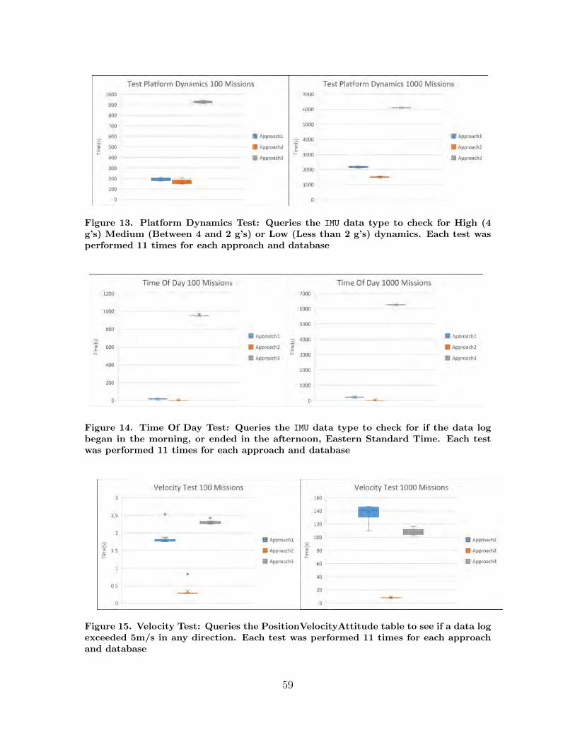
Figure 13. Platform Dynamics Test: Queries the IMU data type to check for High (4g’s) Medium (Between 4 and 2 g’s) or Low (Less than 2 g’s) dynamics. Each test wasperformed 11 times for each approach and database
Figure 14. Time Of Day Test: Queries the IMU data type to check for if the data logbegan in the morning, or ended in the afternoon, Eastern Standard Time. Each testwas performed 11 times for each approach and database
Figure 15. Velocity Test: Queries the PositionVelocityAttitude table to see if a data logexceeded 5m/s in any direction. Each test was performed 11 times for each approachand database
59
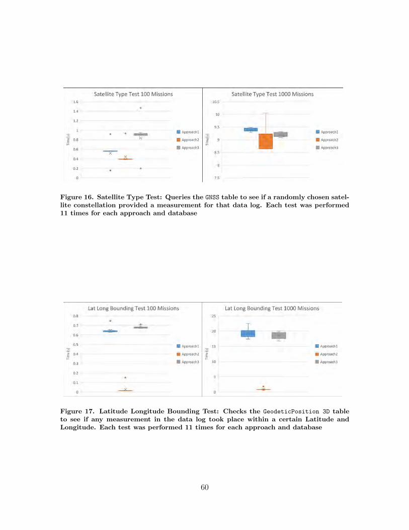
Figure 16. Satellite Type Test: Queries the GNSS table to see if a randomly chosen satel-lite constellation provided a measurement for that data log. Each test was performed11 times for each approach and database
Figure 17. Latitude Longitude Bounding Test: Checks the GeodeticPosition 3D tableto see if any measurement in the data log took place within a certain Latitude andLongitude. Each test was performed 11 times for each approach and database
60
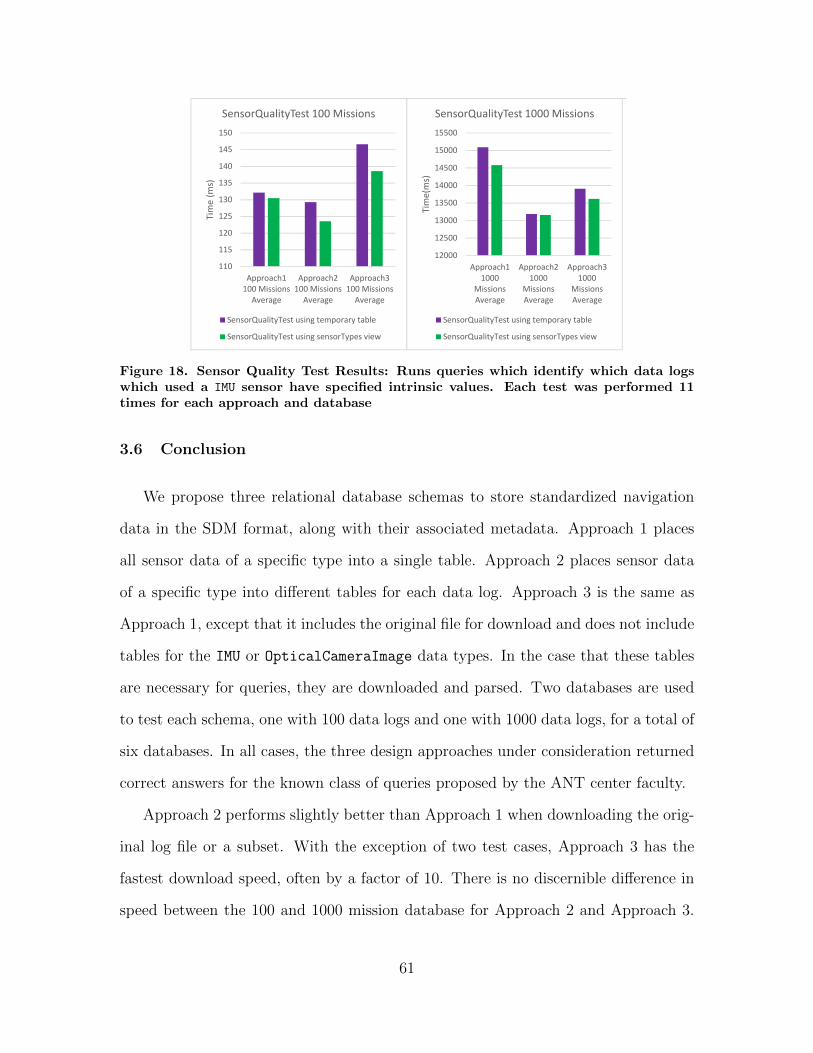
110
115
120
125
130
135
140
145
150
Approach1
100 Missions
Average
Approach2
100 Missions
Average
Approach3
100 Missions
Average
Tim
e (
ms)
SensorQualityTest 100 Missions
SensorQualityTest using temporary table
SensorQualityTest using sensorTypes view
12000
12500
13000
13500
14000
14500
15000
15500
Approach1
1000
Missions
Average
Approach2
1000
Missions
Average
Approach3
1000
Missions
Average
Tim
e(m
s)
SensorQualityTest 1000 Missions
SensorQualityTest using temporary table
SensorQualityTest using sensorTypes view
Figure 18. Sensor Quality Test Results: Runs queries which identify which data logswhich used a IMU sensor have specified intrinsic values. Each test was performed 11times for each approach and database
3.6 Conclusion
We propose three relational database schemas to store standardized navigation
data in the SDM format, along with their associated metadata. Approach 1 places
all sensor data of a specific type into a single table. Approach 2 places sensor data
of a specific type into different tables for each data log. Approach 3 is the same as
Approach 1, except that it includes the original file for download and does not include
tables for the IMU or OpticalCameraImage data types. In the case that these tables
are necessary for queries, they are downloaded and parsed. Two databases are used
to test each schema, one with 100 data logs and one with 1000 data logs, for a total of
six databases. In all cases, the three design approaches under consideration returned
correct answers for the known class of queries proposed by the ANT center faculty.
Approach 2 performs slightly better than Approach 1 when downloading the orig-
inal log file or a subset. With the exception of two test cases, Approach 3 has the
fastest download speed, often by a factor of 10. There is no discernible difference in
speed between the 100 and 1000 mission database for Approach 2 and Approach 3.
61
While Approach 3 has the best performance for download a file, Approach 1 and 2
have acceptable performances, with Approach 2 being faster than Approach 1 by a
few seconds across most test cases.
There are differences in performance for the tests where the SDM sensor data
tables are queried. When the IMU table is queried, both Approaches 1 and 2 out-
perform Approach 3. Approach 3 completes this test for 1000 missions in an hour
and forty minutes, whereas Approaches 2 and 1 complete it in about 25 minutes and
36 minutes, respectively. Approach 2 outperforms Approaches 1 and 3 for all other
SDM tests, with Approach 3 performing about as well as Approach 1 for the data
tests where they share the same schema.
The tests for the non-SDM database tables (Metadata Query Test) demonstrate
that the proposed schema scales well from 100 data logs to 1000 data logs, completing
all but one query in under half a second even for the larger databases, and that
various databases containing randomized data perform similarly well using the same
underlying schema.
These results demonstrate that Approach 2 has the best performance overall for
databases with 100 and 1000 SDM data logs. With Approach 1, some of the SDM
tables become very large at 1000 data logs, such as the IMU table which exceeds 400
million rows. Even though Approach 1 uses indexes, it still loses minutes when these
large tables need to be queried for each data log. Approach 3 has the best performance
when downloading files in most cases, but Approaches 1 and 2 still have acceptable
times that are under a minute for medium and small files. Approach 3, due to the
need to download and parse all files when the data type is unavailable, performed
100’s or 1000’s of times slow in those cases. This performance is prohibitively poor
for Approach 3.
We therefore recommend Approach 2 as the database schema moving forward.
62

Its schema scales, and will make implementation on a distributed database easier
due to the ability to place different tables on different nodes. Users will be able to
choose which subset of missions to run queries against, and will be able to identify
the missions of interest for their specific research interests. Splitting tables will not
be necessary, as would eventually be the case with Approach 1. If space allowed, it
may be advantageous to make the original data logs available for download directly
from the database. In this scenario, the performance for Approach 2 and Approach
3 would be captured in a single database schema.
The next step is implement the database with real data logs and tester-recorded
metadata. This includes designing the distributed aspect of the database, and getting
it live on a cloud server to help with research.
3.7 Database Population
This section was removed from the paper entitled “Relational Database for PNT
Data” due to space restrictions. It presents the methodology used for populating the
test databases.
3.7.1 Log File Ordering
The six databases are populated with SDM data from six LCM files. Files one
through five are parsed and read into the databases repeatedly and consecutively, and
File six is uploaded in place of File one once every 250 missions. The breakdown of
these files for each database is shown in Table 9.
Table 10 shows the respective size of each file, and the total number of LCM events
per file. File 6 is the only file to include OpticalCameraImage messages, which is the
reason that it is many orders of magnitude larger than the other files. Due to space
restrictions, File 6 is repeated less often in the databases.
63
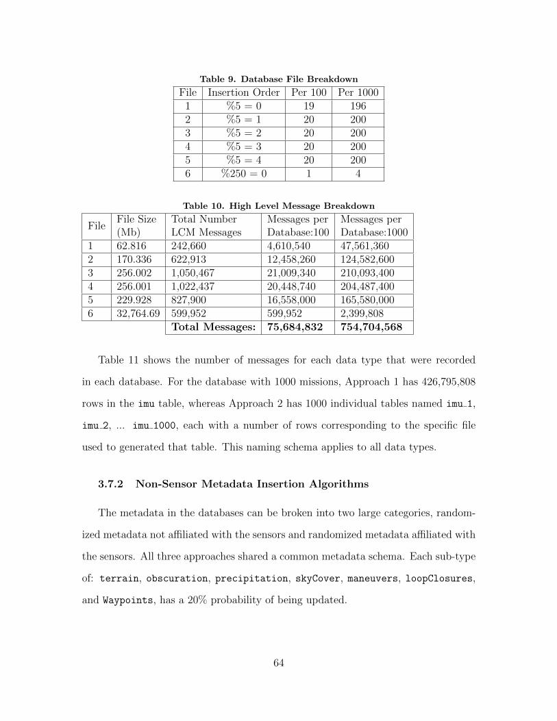
Table 9. Database File Breakdown
File Insertion Order Per 100 Per 10001 %5 = 0 19 1962 %5 = 1 20 2003 %5 = 2 20 2004 %5 = 3 20 2005 %5 = 4 20 2006 %250 = 0 1 4
Table 10. High Level Message Breakdown
FileFile Size(Mb)
Total NumberLCM Messages
Messages perDatabase:100
Messages perDatabase:1000
1 62.816 242,660 4,610,540 47,561,3602 170.336 622,913 12,458,260 124,582,6003 256.002 1,050,467 21,009,340 210,093,4004 256.001 1,022,437 20,448,740 204,487,4005 229.928 827,900 16,558,000 165,580,0006 32,764.69 599,952 599,952 2,399,808
Total Messages: 75,684,832 754,704,568
Table 11 shows the number of messages for each data type that were recorded
in each database. For the database with 1000 missions, Approach 1 has 426,795,808
rows in the imu table, whereas Approach 2 has 1000 individual tables named imu 1,
imu 2, ... imu 1000, each with a number of rows corresponding to the specific file
used to generated that table. This naming schema applies to all data types.
3.7.2 Non-Sensor Metadata Insertion Algorithms
The metadata in the databases can be broken into two large categories, random-
ized metadata not affiliated with the sensors and randomized metadata affiliated with
the sensors. All three approaches shared a common metadata schema. Each sub-type
of: terrain, obscuration, precipitation, skyCover, maneuvers, loopClosures,
and Waypoints, has a 20% probability of being updated.
64
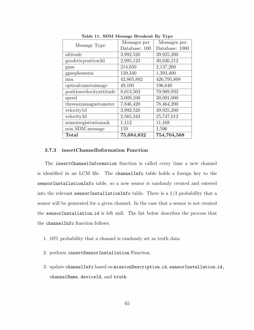
Table 11. SDM Message Breakout By Type
Message TypeMessages perDatabase: 100
Messages perDatabase: 1000
altitude 3,992,520 39,925,200geodeticposition3d 2,995,123 30,026,212gnss 214,650 2,137,200gpsephemeris 139,340 1,393,400imu 42,865,882 426,795,808opticalcameraimage 49,160 196,640positionvelocityattitude 8,013,503 79,989,932speed 3,009,100 30,091,000threeaxismagnetometer 7,846,420 78,464,200velocity1d 3,992,520 39,925,200velocity3d 2,565,343 25,747,012sensorregistrationack 1,112 11,168non SDM message 159 1,596Total 75,684,832 754,704,568
3.7.3 insertChannelInformation Function
The insertChannelInformation function is called every time a new channel
is identified in an LCM file. The channelInfo table holds a foreign key to the
sensorInstallationInfo table, so a new sensor is randomly created and entered
into the relevant sensorInstallationInfo table. There is a 1/3 probability that a
sensor will be generated for a given channel. In the case that a sensor is not created
the sensorInstallation id is left null. The list below describes the process that
the channelInfo function follows.
1. 10% probability that a channel is randomly set as truth data
2. perform insertSensorInstallation Function.
3. update channelInfo based on missionDescription id, sensorInstallation id,
channelName, deviceId, and truth.
65

3.7.4 insertRandomSensorMetadata
The list below walks through the process of populating the sensorMetadata ta-
bles and the sensorInstallation table. The sensorInstallationInfo table holds
foreign keys to their other relevant sensor tables, meaning that appropriate rows need
to either be identified or updated in these other tables so that their keys can be used
to identify or update the appropriate row in the sensorInstallationInfo table.
Once this update is either complete or not performed due to no sensor model being
assigned to this channel, this key or a null value will be returned to the channelInfo
table.
1. insertRandomSensorModel function
2. insertRandomExtrinsicSensorMetadata function
3. insertSensorUID function
4. insertVehicle function
5. Update sensorInstallationInfo table
6. return sensorInstallationInfo id
These functions are discussed below. The entered values are intended to be in the
appropriate format and orders of magnitude expected of actual recorded missions.
• insertRandomSensorModel: For the purposes of this project, there are
eight designated sensor types: BAROMETER, MAGNETOMETER, GNSS, GPS, IMU, IMS,
CLOCK, and CAMERA. There is a 1/24 probability that one of these types will be
assigned to a given channel (with an 8/24 probability that a channel will be
assigned a type at all).
66
• sensorModelId: Takes input with the format: manufacturer, model, and
sensorType, and checks to see if this row already exists in the sensorModelId
table. If not, the function then updates the table with the new row.
• insertRandomExtrinsicSensorMetadata: This function randomly creates
numbers between 0 and 2 for the leverArm, orientationX, orientationY, and
orientationZ matrix columns in the extrinsicSensorConfiguration table.
• insertSensorUID: This function updates the sensoruid column of the sensorSpecific
table. The letters XYZ are combined with a random number from 0 to 99999 to
update the table. Once this update is complete, the insertSensorIntrinsic
table is updated using the new UID as the primary key. If this number already
exists, the UID is returned to be included in the sensorInstallationInfo
table.
• insertSensorIntrinsic: This function updates the IMU Intrinsic table, the
clock Intrinsic table, the camera table, and the GPS Intrinsic table. In
an actual application, only one of these tables would be updated in association
with the specific sensor model and type used to populate the sensorInstallationInfo
table (i.e. an IMU would have IMU Intrinsic data).
• insertVehicle: This function updates the vehicle associated with the specific
channel of interest. For the purposes of this experiment, a different vehicle
may be assigned to each channel, even though in practice the channels in each
LCM log file were each collected by individual vehicles. The vehicle table holds
foreign keys to the aircraft and groundVehicle tables. More may be added
based on how data is collected. The vehicle table recognizes eight types of
vehicles: GROUND VEHICLE, PEDESTRIAN, MISSILE, UAV, SUB, and AIRCRAFT.
67
3.7.5 insertSDMData
The specific details of inserting SDM data into a database vary by the data type.
There are thirteen individual functions, one for each SDM data type and two addi-
tional for sensorRegistrationAck and for non sdm data. In general, data is read
out of each LCM event and then written directly into the database using a prepared
statement.
1. identify message type
2. identify message channel name
3. insert new channel information into channelInfo
4. insert message data in SDM table
Most of the work around Approach 1 and Approach 2 download test is centered on
the GenericFetchEventBundle class. This class is initialized according to the specific
SDM data type and the table name. If the database of interest is based on Approach
2, the table name will have the format sdmDataType missionDescription id. For
example, if the data type is IMU and the mission id is 737, the table name will be
imu 737. The main purpose for the GenericFetchEventBundle class is to provide a
convenient wrapper for a series of SQL queries which allow the LCM events of the
original log file to be created. This allows them to be written back to a log file,
creating the original log file or a subset. Thus the following query is an example for
the imu table, the g.delta v and g.delta theta data types would be replaced with
those of the appropriate types for the given table of interest.
1 SELECT2 c.channelname ,3 g.utime ,4 g.eventNumber ,5 c.deviceid ,6 g.timestamp_arrival_sec ,
68

7 g.timestamp_arrival_nsec ,8 g.timestamp_valid_sec ,9 g.timestamp_valid_nsec ,
10 g.seqnumber ,11 g.delta_v ,12 g.delta_theta ,13 FROM14 "channelInfo" c15 INNER JOIN16 imu g17 ON g.channel_id = c.id18 WHERE19 g.id BETWEEN (next_sdm_id) AND20 (21 next_sdm_id + bundle_size - 122 )23 ;
Note that the SENSOR REGISTRATION ACK and NON SDM MESSAGE have different
headers from the other SDM data types due to different available information in
the original LCM events. For these, the header becomes:
1 SELECT2 c.channelname ,3 g.utime ,4 g.eventNumber
and excludes the additional information leading up to the table-specific columns
The GenericFetchEventBundle class is ultimately designed to return bundles of
completed events of the appropriate data type. The bundle size is set to 100,000
for all data types except for OpticalCameraImage, which is set to 1 (so as to avoid
an OutOfMemoryError Exception). When this class is created as an object, a list
of Strings called columnNames is initialized with the appropriate SDM data types
according to the table columns of interest. The setEventsBundle Function informs
the GenericFetchEventBundle of the missionDescription id and bundle size,
passes in the database Connection, and further defines the specific channels and
minimum and maximum ids of the table of interest. Table 12 shows a list of attributes
of the GenericFetchEventBundle class and Table 13 shows the operations for this
class.
69
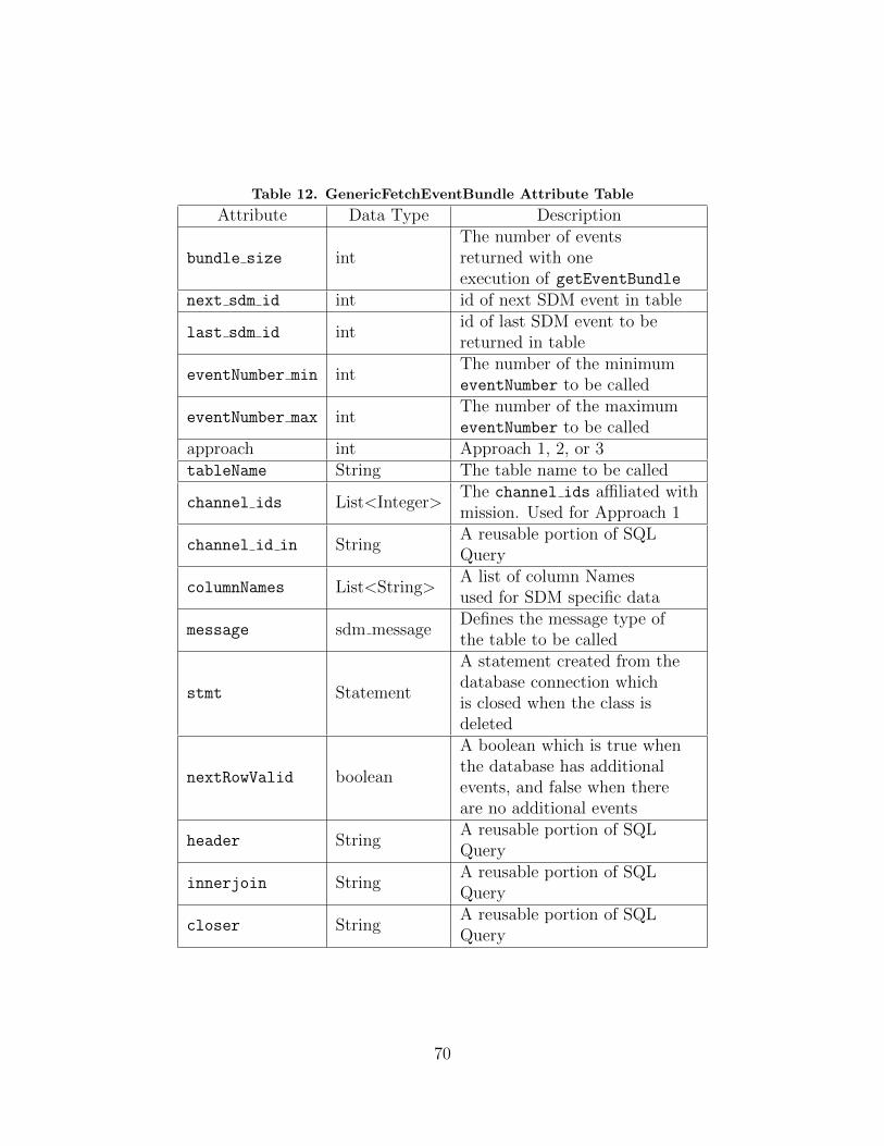
Table 12. GenericFetchEventBundle Attribute Table
Attribute Data Type Description
bundle size intThe number of eventsreturned with oneexecution of getEventBundle
next sdm id int id of next SDM event in table
last sdm id intid of last SDM event to bereturned in table
eventNumber min intThe number of the minimumeventNumber to be called
eventNumber max intThe number of the maximumeventNumber to be called
approach int Approach 1, 2, or 3tableName String The table name to be called
channel ids List<Integer>The channel ids affiliated withmission. Used for Approach 1
channel id in StringA reusable portion of SQLQuery
columnNames List<String>A list of column Namesused for SDM specific data
message sdm messageDefines the message type ofthe table to be called
stmt Statement
A statement created from thedatabase connection whichis closed when the class isdeleted
nextRowValid boolean
A boolean which is true whenthe database has additionalevents, and false when thereare no additional events
header StringA reusable portion of SQLQuery
innerjoin StringA reusable portion of SQLQuery
closer StringA reusable portion of SQLQuery
70
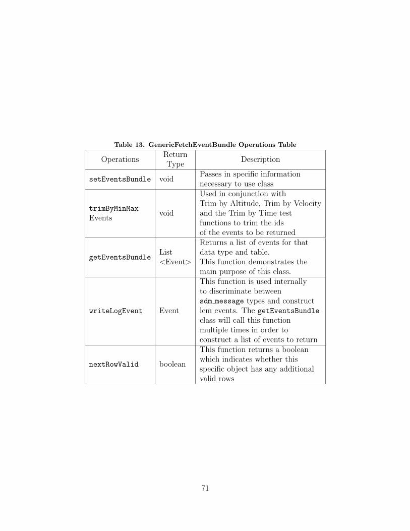
Table 13. GenericFetchEventBundle Operations Table
OperationsReturnType
Description
setEventsBundle voidPasses in specific informationnecessary to use class
trimByMinMax
Eventsvoid
Used in conjunction withTrim by Altitude, Trim by Velocityand the Trim by Time testfunctions to trim the idsof the events to be returned
getEventsBundleList<Event>
Returns a list of events for thatdata type and table.This function demonstrates themain purpose of this class.
writeLogEvent Event
This function is used internallyto discriminate betweensdm message types and constructlcm events. The getEventsBundle
class will call this functionmultiple times in order toconstruct a list of events to return
nextRowValid boolean
This function returns a booleanwhich indicates whether thisspecific object has any additionalvalid rows
71

3.8 Indexes
This section was removed from the paper entitled “Relational Database for PNT
Data” due to space restrictions.
Due to early experimentation showing significant slow downs for queries on the
SDM tables for Approaches 1 and 3, indexes are added for each SDM table. These
indexes are on the channel id, eventnumber, and the table id. Each are discussed
in Table 14. Including these indexes allows for a convenient sequence of SQL queries
which allows an automated program to readily identify the beginning and ending ids
for a given SDM table which correspond to a specific mission. For Approach 1 and
Approach 2, the ids are ever increasing, however the eventNumbers always start at a
low number and end at a high number (corresponding to whatever the first and last
eventNumbers are for that data type and mission in the original LCM log file).
The results listed in section 4 include these indexes. An example of the SQL DDL
to create one of these indexes for the imu table is as follows:
1 CREATE INDEX imu_eventnumber_id2 ON imu (channel_id , eventnumber , id);3 ntNumber
The following sequence of SQL demonstrates the query series utilized to determine
the beginning and ending ids of an SDM table for a specific mission. For Approach
2 the first and last ids of the table and mission of interest are just identified directly,
as they only correspond to that specific mission.
1 SELECT DISTINCT2 (id)3 FROM4 "channelInfo"5 WHERE6 missionDescription_id = ? ;7 SELECT8 min_max (eventNumber)9 FROM
10 "tableName"11 WHERE12 channel_id IN13 (14 ?,
72

Table 14. SDM Common Columns Subset
Column Name Column Description
id
An integer description of a uniquerow in an sdm table. This integerautoincrements as each additionalrow is added
eventNumberA number which describes messageorder in the original LCM log file
channel id
A number which describes which channelan sdm message was transmitted on. Thisnumber allows messages to be linkedback to the original missionDescription id
utimeThe utime when the message was transmittedin microseconds. This number will be usedto determine timing in queries.
15 ?,16 ...,17 ?18 )19 ;20 SELECT21 min_max(id)22 FROM23 "tableName"24 WHERE25 channel_id IN26 (27 ?,28 ?,29 ...,30 ?31 )32 AND33 (34 eventNumber = ?35 )36 ;
3.9 Removed Metadata Query Test Figures
Figures 19, 20 and 21 were removed from the ION/PLANS paper due to space
restrictions.
73
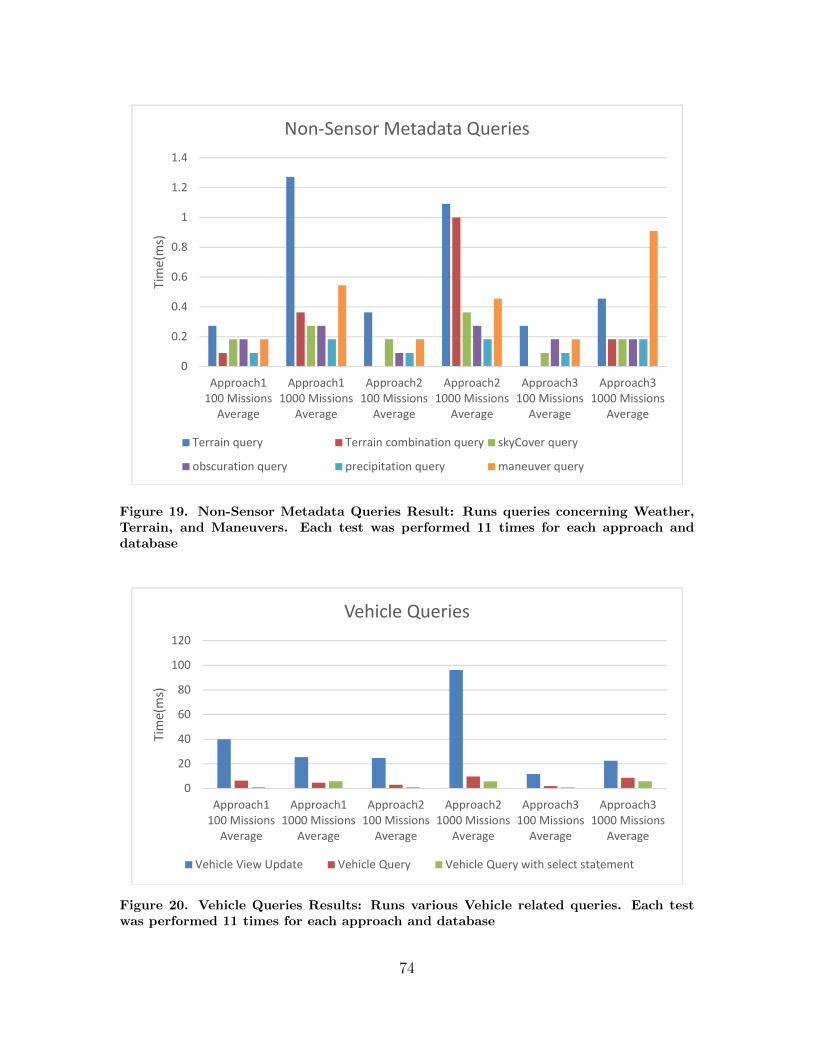
0
0.2
0.4
0.6
0.8
1
1.2
1.4
Approach1
100 Missions
Average
Approach1
1000 Missions
Average
Approach2
100 Missions
Average
Approach2
1000 Missions
Average
Approach3
100 Missions
Average
Approach3
1000 Missions
Average
Tim
e(m
s)
Non-Sensor Metadata Queries
Terrain query Terrain combination query skyCover query
obscuration query precipitation query maneuver query
Figure 19. Non-Sensor Metadata Queries Result: Runs queries concerning Weather,Terrain, and Maneuvers. Each test was performed 11 times for each approach anddatabase
0
20
40
60
80
100
120
Approach1
100 Missions
Average
Approach1
1000 Missions
Average
Approach2
100 Missions
Average
Approach2
1000 Missions
Average
Approach3
100 Missions
Average
Approach3
1000 Missions
Average
Tim
e(m
s)
Vehicle Queries
Vehicle View Update Vehicle Query Vehicle Query with select statement
Figure 20. Vehicle Queries Results: Runs various Vehicle related queries. Each testwas performed 11 times for each approach and database
74

0
20
40
60
80
100
120
140
160
Approach1 100
Missions Average
Approach1 1000
Missions Average
Approach2 100
Missions Average
Approach2 1000
Missions Average
Approach3 100
Missions Average
Approach3 1000
Missions Average
Tim
e (
ms)
Sensor Type Queries
sensorType View update Type query using sensorTypes View
Type combination query using sensorTypesView Type Query using SELECT statement
Type combination query defining a temporary table
Figure 21. Sensor Type Test Results: Runs various Sensor Type related queries, as wellas queries looking for random combinations of two sensor. Each test was performed 11times for each approach and database
75

IV. Experimental Scenarios
4.1 Journal Of Evolutionary Computation Paper
This section consists of a paper which will be submitted to the Journal of Evolu-
tionary Computation entitled ”Multi-Objective Database Queries in Combined Knap-
sack and Set Covering Problem Domains.” This paper addresses the combined MO
KP/SCP and two stochastic algorithms which return solutions to complex queries for
the database discussed in Section 3.
Consider a relational database that is designed to organize PNT metadata specif-
ically related to test flights which were conducted by the AFIT. AFIT has approx-
imately 100 data logs (also called missions) which will be stored in this relational
database. This database requires a number of queries from parties interested in using
this data for research.
Two relevant well-known NP-Complete problems are the 0/1 KP and the 0/1 SCP
[76] [77] [78] [79]. The terms 0 and 1 indicate that, given a Problem Domain (PD)
of objects, each object is either included in a specific solution (1), or excluded (0).
An answer in this PD is one that meets all of the problem constraints, and a global
optimum is one that has a better objective function then all other solutions in the
search space [80]. The specific details of the KP PD, the SCP PD, and the combined
KP/SCP PD is provided in Section 4.4.
Consider the following brief description of the combined MO KP/SCP when con-
verted to a database query: “Return the set of data logs where at least one data log
meets n different criteria, and for which at least one each of x category are utilized
with the summation of z number totaling no more than c number, and maximizing
k.” A specific implementation of this query may be: Return the set of data logs
where a given set of sensor types and terrain types are represented across the set
76

of returned data logs, and where the number of sensor readings recorded over 1000
meters in altitude across all data logs is maximized, and the total summed time of
all data logs does not exceed 2 hours.
To the best knowledge of computer scientists today, problems which are NP-
Complete do not have available polynomial time algorithms [78], and for that reason
stochastic-algorithms and metaheuristics are used to find approximate answers [80]
[81]. This paper proposes a Genetic Algorithm (GA) stochastic population based
search algorithm and a Hill Climber (HC) stochastic local search algorithm to return
answers to this problem domain. Both are based on a GA developed by Beasley and
Chu (1996) [82], and utilize modified code based on work by Cobonkerr(2020) [83].
These algorithms are tested against two relational databases, one with 100 navi-
gation data logs, and one with 1000 data logs. These databases are populated with
six files of repeated sensor data in the SDM format, which is discussed in Section 4.3,
and randomly entered metadata. They are implemented in Java, and use SQL queries
to populate Java data structures, which then run the algorithms and return answers
to the NP-Hard combined MO KP/SCP. In application, this Java program functions
as part of the User Interface, and would interact with the underlying database on
behalf of the researcher. The benefit is that the queries are simple, but allow for
more complex results to be returned. The queries in the next section could modified
at will. As long as the input to the MO KP/SCP implementations fits the format
defined in this paper, it allows for any sub-queries to populate the relevant problem
data structures.
The applications of NP-Hard combinatorial problems is well recognized in the
literature [80] [84] [85] [86]. Rosendo and Pozo (2010) [87] discuss the application of
particle swarm optimization with respect to Database vertical partitioning. Vertical
partitioning optimization is critical with regards to speeding up user queries that may
77
be spread across multiple fragments of a database.
A preliminary literature review did not discover other studies with comparable
results to those laid out here, nor did it uncover the combination of the KP and SCP.
However, Balke and Guntzer (2004) wrote an article which highlighted optimization
and constraint concerns for MO queries of databases which are similar to those pro-
posed by this paper. They specify cite real estate queries and web information services
as examples of databases where customers may have competing priorities that require
optimization [55]. Specific comparative examples of these conflicting examples will
come along as this PNT database is used by researchers with varying interests. This
paper as it is written describes one possible application of a MO query.
Section 4.2 discusses the background of the relational databases used to test the
stochastic algorithms. Section 4.3 discusses the PD of the SCP and the KP, and
the combined KP/SCP. Section 4.4 develops the pseudo code for the GA and the
HC. Section 4.5 presents the test experiment and section 4.6 provides the experiment
results. Section 4.7 is the paper conclusion.
4.2 Background and Related Queries
This section covers some specific details of the database design in order to motivate
how the SCP and KP can combine to help facilitate database queries. This database
is implemented in PostgreSQL, which is an open source, object-relational database
system which dates back to 1986 at the University of California at Berkely. This
RDBMS supports arrays and documents (such as JSON), is also extensible, in that
additional data types, functions, and operators can be added [39].
Three potential PostgreSQL relational database designs are compared to store
PNT data [67]. These designs offer identical ways to store sensor metadata and non-
sensor metadata, and differing ways to store sensor data which is recorded in the
78
SDM format. A database overview from [67] is shown in Figure 22:
The missionDescription table in the overview above depicts the various missions
stored in the database. In other words, a row in the missionDescription table,
along with all of the other data related to that row in the children tables, together
comprise all of the available information for that mission. The Sensor Metadata
table is coupled with the channelInfo table so that specific sensors can be affiliated
with channels for a given mission, and the SDM Data tables are comprised of the data
collected by those sensors. For the chosen approach, a new table is created for each
SDM data type and for each mission. Kauffman et al. (2017, 2020) provide additional
background on the data available in Table 15. (Mochocki, 2020) goes into additional
detail on the tests which discriminated between these three solutions, and provides
rational for the solution chosen to meet AFIT’s data storage needs [7] [74].
For each approach, two databases were created, one with 100 missions and one
with 1000 missions, in order to help show how these approaches scale as they become
larger. The missions are composed of six log files in the LCM format, which are
uploaded repeatedly into the databases, along with randomized sensor and non-sensor
metadata which are associated with each data log.
In order to populate the data structures discussed later in this article, a series of
SQL queries are used in conjunction with the PNT database. The following queries
are written for the chosen database design and are discussed here, along with their
use in populating data for this algorithm:
1 SELECT2 MAX (id)3 FROM4 missionDescription;
Purpose: Every mission is a column which may be part of a returned solution. This
query identifies the number of missions in the database and updates the total number
of columns in the problem based on this number
1 SELECT
79
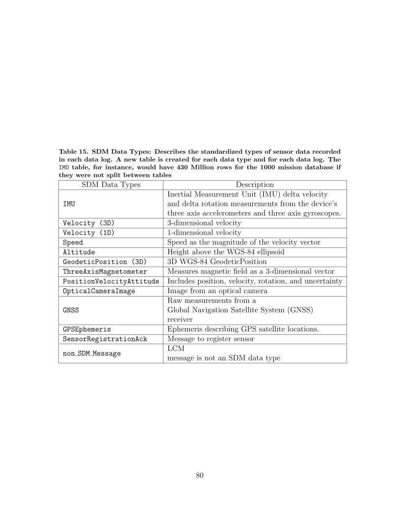
Table 15. SDM Data Types: Describes the standardized types of sensor data recordedin each data log. A new table is created for each data type and for each data log. TheIMU table, for instance, would have 430 Million rows for the 1000 mission database ifthey were not split between tables
SDM Data Types Description
IMU
Inertial Measurement Unit (IMU) delta velocityand delta rotation measurements from the device’sthree axis accelerometers and three axis gyroscopes.
Velocity (3D) 3-dimensional velocityVelocity (1D) 1-dimensional velocitySpeed Speed as the magnitude of the velocity vectorAltitude Height above the WGS-84 ellipsoidGeodeticPosition (3D) 3D WGS-84 GeodeticPositionThreeAxisMagnetometer Measures magnetic field as a 3-dimensional vector
PositionVelocityAttitude Includes position, velocity, rotation, and uncertaintyOpticalCameraImage Image from an optical camera
GNSS
Raw measurements from aGlobal Navigation Satellite System (GNSS)receiver
GPSEphemeris Ephemeris describing GPS satellite locations.SensorRegistrationAck Message to register sensor
non SDM MessageLCMmessage is not an SDM data type
80
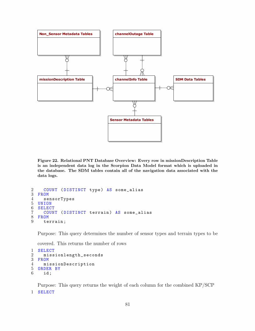
missionDescription Table
Non_Sensor Metadata Tables
channelInfo Table
Sensor Metadata Tables
SDM Data Tables
channelOutage Table
Figure 22. Relational PNT Database Overview: Every row in missionDescription Tableis an independent data log in the Scorpion Data Model format which is uploaded inthe database. The SDM tables contain all of the navigation data associated with thedata logs.
2 COUNT (DISTINCT type) AS some_alias3 FROM4 sensorTypes5 UNION6 SELECT7 COUNT (DISTINCT terrain) AS some_alias8 FROM9 terrain;
Purpose: This query determines the number of sensor types and terrain types to be
covered. This returns the number of rows
1 SELECT2 missionlength_seconds3 FROM4 missionDescription5 ORDER BY6 id;
Purpose: This query returns the weight of each column for the combined KP/SCP
1 SELECT
81

2 c.missionDescription_id ,3 MAX(e.eventNumber) - MIN(g.eventNumber)4 AS value5 FROM geodeticposition3d_? g6 INNER JOIN7 channelInfo c8 ON c.id = g.channel_id9 WHERE g.altitude > 1000
10 AND c.missionDescription_id BETWEEN 1 AND numColumns11 GROUP BY12 c.missionDescription_id;
Purpose: This query returns the value of each column for the combined KP/SCP.
The GeodeticPosition (3D) data type is chosen to determine the minimum and
maximum event numbers because it is a common data type which exists across most
missions
12 SELECT3 id,4 type5 FROM6 sensorTypes7 ORDER BY8 id;
Purpose: This query returns a list of sensor types and their associated mission iden-
tifiers. These are the first eight rows to be covered by the KP/SCP
12 SELECT3 missionDescription_id ,4 terrain5 FROM6 terrain7 ORDER BY8 missionDescription_id;
Purpose: This query returns a list of terrains and their associated mission identifiers.
These are the last 5 rows to be covered by the KP/SCP.
These queries take time and have an overhead observable in the testing data.
They take approximately 2 seconds to complete for the 100 mission database, and
17 seconds to complete for the 1000 mission database. This will help contextualize
the performance of the GA and HC algorithms. The next two sections of this paper
82

discuss the combined KP/SCP PDs, and the GA and HC algorithm.
4.3 Problem Domain
In order to define how the problem space of the SCP and KP combine, each one
is defined individually. Following this, their combination is addressed.
4.3.1 Set Covering Problem
The general SCP entails having a group of sets which are to be covered (defining
the universe), and a group of families, each which is composed of a subset of sets, so
that a complete covering of the sets is composed of a group of families, the combined
sets of which include all of the sets to be covered. According to [88] the SCP is defined
as:
Set Covering Problem: Given a set R = {r1, ..., rm} and a family F = {S1, ..., SN}
of sets Sj ⊂ R any subfamily F ′ = {Sj1, Sj2, ...Sjk} of F such that ∪ki=1 Sji = R
is called a subset covering of R, and the Sji are called the covering sets.
According to Caprara et al. (2000) , SCP can be thought of in terms of [76]:
Ji = {j ∈ J : aij = 1}
Ij = {i ∈ I : aij = 1}
which describes the columns which cover the rows and the rows which are covered by
the columns. This concept is applied in code by defining two dimensional array lists
in Java.
83

Typically the SCP is thought of as having costs such that the goal is to Minimize
∑j∈J
cjxj
which means that the families chosen to be part of the solution have associated costs
which are to be minimized. This minimization is part of the optimization process.
Solution Space: The SCP is O(2n) [89]. This is due to a full solution having to
consider all possible combinations of the available sets.
Problem Class: NP-Complete [78].
The SCP can be framed as a query for the PNT database described in Sections
3.2 and 4.3: Return a subset of data logs that minimize the total summed time of the
missions such that all terrain types and sensor types are represented.
4.3.2 The Knapsack Problem
In the general form of the KP problem, objects have an associated weight and
value which are not (necessarily) related, and bins have a certain weight capacity. An
optimal answer returns the set of items that fit in this bin that have the maximum
value.
84
Knapsack Problem: Given a set of n items. Each item i = 1...n has two parameters,
a weight wi and a value vi. Given a knapsack capacity X, find a subset Xof items
of maximum value that does not exceed the weight restriction. The goal is to
maximize∑i∈S
vi such that∑i∈S
wi ≤ X [78].
Solution Space: The KP is O(2n). This is due to a full solution having to consider
all possible combinations of the available sets [78].
Problem Class: NP-Complete [78].
The KP can be framed as a query for the PNT database described in Sections 3.2 and
3.3: Return a subset of data logs where the total summed time of missions does not
exceed X seconds, and where the total number of sensor measurements taken above
Y altitude are maximized.
4.3.3 Combined Problem
Find a solution such that both problem domains are satisfied and optimized. SQL
queries are used against the PNT database to populate data structures affiliated
with the combined KP/SCP. These data structures are used with conjunction with a
Population (GA) and Local Search (HC) algorithm to return answers to the queries
in the combined KP/SCP problem domains.
English Description: Given a knapsack capacity, a set of rows to be covered,
and a set of families which each have some subset of these rows, and also have an
associated value and weight. Return a subset of these families which covers all of
85
these rows (combinatorial problem, one type of optimization), and for which the
combined weight does not exceed the knapsack capacity (constraint), and which has
the maximum possible combined value for the sets (optimization).
The KP/SCP: Given a capacity X, a set R = {r1, ...rm}, and a family F = {S1, ...SN}
of sets Sj ⊂ R and associated weights Fw = {w1, ..., wN} and values Fv = {v1, ...vN},
return a subfamily F ′ = {Sj1, Sj2, ...Sjk} of F such that ∪ki=1 Sji = R, which
maximizes∑i∈F
vi such that∑i∈F
wi ≤ X and for which @[(Sn)|Sn ⊂ (F ′ − Sn)]
The goal in this problem domain is to optimize the combined value
∑i∈F
vi (2)
and to provide a set covering such that
∪ki=1Sji = R
The weight
FW = {w1, ...wN}
can be thought of in terms of the cost from the original SCP problem, but this is not
a perfect corollary. For instance, it does not matter if
∑i∈F
wi = X
or if the combined weight is arbitrarily lower, so just trying to minimize weight is
not necessarily an optimization goal. The goal is to provide a set covering so that
86

value is maximized, while not exceeding the aforementioned constraints. These are
competing optimizations, as there may be solutions to the Knapsack Problem which
have higher values yet which do not provide a set cover, and there may be smaller set
coverings with lower weights which provide less value.
Solution Space: Both of these problems could be solved independently if the rele-
vant parameters from the other problem were ignored. Even so, each is a permutation
problem, resulting in them having equivalently sized solution spaces. Therefore this
problem has a solution space of O(2n), which is the same as if they were solved inde-
pendently.
Problem Class: The KP/SCP PD can be thought of as a decision problem. For a
given answer to a SCP, is it a valid minimal set cover that meets the three combined
conditions:
∪ki=1Sji = R (3)
@[(Sn)|Sn ⊂ (F ′ − Sn)] (4)
∑i∈F
wi ≤ X (5)
The SCP decision problem reduces to the combined KP/SCP Problem. A proof
is available in Mochocki (2020) [67]. This shows that the KP/SCP decision problem
is NP-Complete. The KP/SCP problem is likely NP-Hard, as it would be difficult
to provide a polynomial time certifier that a given answer is indeed optimal. The
next section describes the top down design of algorithms to solve the combined MO
KP/SCP. The SQL queries in Section 3.3 are used to populate data structures, which
are used with these algorithms to return answers to this PD.
87

4.4 Stochastic Algorithms for the Combined MO KP/SCP
The code for the GA and HC algorithms sections are based on the work by
Cobonkerr (2020), which implements the algorithm designed by Chu and Beasley
(1997)[83] [90]. Some sections of the code required major rewrites to implement the
modified algorithms. The pseudo code is available in the appendix of Mochocki (2020)
[67].
4.4.1 Genetic Algorithm
Consider the general description of a GA [91]:
1. Initialize a population of chromosomes; (Set of Candidates)
2. Evaluate each chromosome in the population; (Feasibility)
3. Create new chromosomes by mating current chromosomes – apply mutation and
recombination as the chromosome mate; (Next State Generator)
4. Evaluate the new chromosomes (Feasibility) and insert them into the popula-
tion; (Objective Function)
5. If time is up, stop and return the best chromosome; (Solution), if not, goto 3.
Encoding: Utilize a binary encoding (0/1) for each column to indicate whether or not
that specific column is considered as part of a given solution. Each column has an
associate weight and value. A specific solution is represented as a genome (equivalent
to a chromosome).
Initial Population (Set of Candidates): This is generated at the beginning of the
program based on the specific column/row/weight/value parameters. Each member
88

of the population is checked for feasibility, as detailed below, and to ensure lack of
redundancy between answers.
Training Solutions (Next State Generator):
• Use a k-ary tournament selection to select two parents, each is the most fit
of its respective tournament (participants are randomly selected). [80]. This
approach gives preference to the more fit parent, but does not guarantee that
a bit from that parent is selected.
• Perform a crossover between the two parents to produce a child. Consider each
bit in parents. If bits match, pass bit to child. If bits do not match: Generate
fitness number: fprob = fp2fp1+fp2
. Generate a random number r with the range
0...(fp1 + fp2).
• if r > fprob take the bit from p2 else p1.
• Perform a mutation on the child to produce a new solution. Select a random
bit from child and flip
• Check the child for feasibility, perform a modification on the child to make
feasible
• Add the child back to the population, replacing a less fit member. Calculate
average fitness of population pa = (∑n
i=1 vi1n) . Randomly choose a member of
population. If vm ≤ pa replace, else choose a new member.
Feasibility: The feasibility of the population is checked once generated, and every
new possible solution is checked before being returned to the population.
89

• Per the SCP, the set of rows which are part of the solution need to be checked
to confirm that every row is covered.
• The answer needs to be a minimal subset so that there is no column for which
every covered row is a subset of the rows covered by all of the other combined
columns.
• The combined weight of all columns needs to not exceed the weight restriction.
Mathematically, feasibility is defined as:
1. ∪ki=1Sji = R
2. @[(S)|S ⊂ (F ′ − S)]
3.∑
i∈F wi ≤ X
In the case a given solution is not feasible, it is fixed or discarded deterministically.
Note, it is assumed that Feasibility Condition 2 can only occur if Feasibility Condi-
tion 1 is valid. In other words, a solution cannot be a minimal SCP if it is not an SCP.
Make Feasible: Consider cases in Table 16
Case Descriptions:
(a) All three conditions are true. This means that the solution is feasible. Return
genome.
(b) Min SCP conditions are satisfied but KP condition is not. Discard this genome.
(c) Answer is a SCP and satisfies KP, but is not minimal. Identify redundant family
of lowest value (if multiple) and delete. Return modified genome.
90

Table 16. Genetic Algorithm Possible Feasibility Conditions
Case 1 2 3a T T Tb T T Fc T F Td T F Fe F T Tf F T Fg F F Th F F F
(d) Answer is a SCP but there are redundant columns and KP weight condition is
violated. Identify redundant columns and remove so that weight falls within
restriction. If weight still exceeds limit even once all possible columns are re-
moved, discard this genome.
(e) The solution is not a set cover but the columns proposed so far do not violate
weight limits. See if any columns can be added which meet condition 1 without
violating the weight restriction. Then check for redundancy with added rows.
(f) The solution is not a set cover and it busts the weight limits. Discard this
genome.
(g) Condition 2 assumes that condition 1 is valid, so this combination is meaning-
less.
(h) Condition 2 assumes that condition 1 is valid, so this combination is meaning-
less.
Fitness (Objective Function): Assuming that all solutions are feasible, the best an-
swer, also called the most fit, is the one with the highest value.
91

Convergence:
1. Hard time restriction: This value can be set as a problem parameter and sets
a limit to for how long the algorithm will continue to hunt for better solutions
even while these solutions are actively being found. This time restriction is only
checked in between attempts to evolve new solutions, it will not interrupt an
evolution attempt.
2. Population fitness has not changed in at least 60 iterations. This implies that
a more fit solution is relatively difficult to find.
4.4.2 Hill Climber Algorithm
The Hill Climber Algorithm uses the same problem encoding, queries, and gen-
eration of the initial solution as the GA. The main difference is that the HC only
generates a single solution, and then explores the neighborhood of that solution look-
ing for better answers, terminating when it is completely explored.
Encoding: Use a binary encoding (0/1) for each column/item to indicate whether or
not that specific column is considered as part of a given solution. Each column/item
also has an associated weight and value.
Neighborhood: A given subfamily F ′ = {Sj1, SJ2, ..., Sjk} of F such that ∪ki=1Sji = R
and feasibility constraints are met, subject to all possible Swap combinations O(n2).
Initial Population (Set of Candidates): A single solution S0 is generated as the initial
solution. The generation of this solution matches the process described for the GA.
92

Next State Generator: Utilize swap operation. ∀F (S1, ..., SN) if Sj =“1” and Sk =
“0” Swap (Sj, Sk). Then check for feasibility
Feasibility: The solution encoding is identical to the GA. Therefore, the constraints
and challenges associated with the feasibility of a particular swap operation are the
same. The feasibility function returns either the ∅ or Sjn.
Selection: If Ft+1 > Ft, Make St+1 the new current state, else, discard St+1 and gen-
erate a new next solution per Next State Generator
Solution: Terminate either when: t = T , i.e. a defined amount of time has elapsed or
entire neighborhood has been explored and no better solution returned.
Fitness (i.e. Objective Function): Assuming that all solutions are feasible, the best
answer (i.e. most fit) is the one with the highest value.
4.4.3 GA and HC Algorithm Expected Performance
Section 4.4 laid out the background for the GA and the HC pseudo code. The
key difference between them is that the GA uses a population based approach, k-ary
tournament selection, a fitness-based crossover, mutation, and returns the genome to
the population based on a fitness comparison with the genome to be replaced. The GA
does not run the risk of getting stuck in a single neighborhood, even though the fittest
answers may trend towards a local maximum, and not reach the absolute maximum
which may be somewhere else in the solution space, especially if the crossover and
mutation operators alone are not able to get any of the genomes in the population
there.
93

The Hill Climber explores a specific neighborhood, which is defined as the swap of
all bits for a randomly generated started genome. The make feasible function of the
GA is used only for the generation of the initial solution, any non-feasible solutions
for the HC are discarded, even if they might potentially lead to more fit answers.
Functionally, the HC uses much of the structure of the GA.
Based on their design, we expect that the GA will in general produce more fit
answers to the combined MO SCP/KP in comparison to the HC. The GA is not
restricted to a particular neighborhood, and multiple neighborhoods may be repre-
sented in the population. The HC is expected to find its solutions faster than the GA.
Once the initial solution is discovered, the HC deterministically searches its neigh-
borhood in polynomial time, whereas the GA stochastically generates the entirety of
its initial population before beginning to the genome mutation process.
In Section 4.5, the GA is tested with populations of 10, 25, and 50 genomes
for the 100 and 1000 mission databases. The PD search space represented by the
two databases used to test these algorithms is critical when comparing how the GA
performs between population sizes. As is discussed in the next section, these databases
are composed of repeated files and randomized metadata, with values and weights
stochastically modified after being queried to add nuance to the search space. Even
so, certain combinations of files with high value and low weight are expected to be
present in most answers, especially as the weight limits increase, so it is expected
that GAs with population sizes of 50 will produce similarly fit solutions as the GAs
with a population sizes of 10. In general, for populations that use a binary encoding
smaller population sizes are sufficient to find relatively fit answers [92]. For complex
search spaces (with multiple local maxima) there is not a direct correlation between
population size and the fitness of the returned answers [93].
94

4.5 Design and Evaluation of Experiments
In general, the goals of the experiments are:
1. To validate the functioning of the code and the underlying algorithm implemen-
tation
2. To demonstrate timeliness of execution and the quality of the answers
3. To compare the various implementations
4. To learn about algorithm execution, and to help design potential future work
The two databases that the GA and HC algorithm interface with are composed
of six separate files which were replicated 100 times and 1000 times. This replication
means that there are a predictably finite number of value and weight combinations,
which are derived directly from the SDM data. As the sensor and terrain metadata
is randomly entered, the Set Covering portion of each mission varies. Table 17 shows
the value and weight of the six data logs replicated in the databases:
As is discussed in Section 4.2, the value is the number of recorded events from the
GeodeticPosition (3D) table above 1000 meters and the weight is the total number
of seconds of the mission. While these are specific units, the result of any query could
Table 17. Missions Value and Weight Based On SQL Queries
Mission Value Weight1 418,653 49402 606,444 47433 1,036,695 47434 694,528 52295 712,219 53116 231,187 1837
95

replace these in the algorithm depending on what the researcher is attempting to
optimize.
In order to prevent the algorithm from converging prematurely due to a lack of
potential higher value answers, the value and weight are randomly altered before
being added to the problem data structure. The values of the columns are assigned
± 200,000, and the weights of the columns are assigned ± 1,000 in comparison to
what is shown in Table 17. As this adds an additional element of randomness to
algorithms which are already stochastic in nature, the Genetic Algorithm and Hill
Climber Algorithm are compared on the basis of trends in performance, and not on
individual experiments. Each experiment is repeated 10 times.
In general, each algorithm performs as expected. For a given Weight Limit, the
Hill Climber Algorithm tends to return less fit answers in a faster time, and the
Genetic Algorithm tends to return more fit answers in a slower time. The population
size does not produce much variation in returned value. All testing is done on the
laptop shown in Table 18:
Both the Genetic and the Hill Climber Algorithms are tested against Weight
Limits of 6,000, 10,000, and 20,000, and against the databases with 100 missions and
with 1000 missions. Furthermore, the Genetic Algorithm is tested with populations
Table 18. Testing Equipment and Software
Manufacturer LenovoModel ThinkPad P52 20M9
ProcessorIntel(R) Core(TM)i7-8750H CPU @ 2.20GHz
Installed memory 40GB
System typeWindows 10 Pro64 Bit Processing System
SSD Samsung SSD 970 EVO Plus 2TBIDE Eclipse Version 2019-09 R (4.13.0)RDBMS PostgreSQL 11.6
96

of 10, 25, and 50 elements. Figure 23 Compares how the GA performed for trials
with variations in population and database size.
The population size does not consistently impact the final fitness of the returned
solution for a given weight or database size. With a weight limit of 6,000 and a
database size of 1,000, the population of 50 slightly outperforms the population size
of 25, while with a database size of 1,000 and weight limit of 10,000, the other two
population sizes slightly outperform the population size of 50. In general, with the
larger database, the variances of the population sizes were more compact and more
similar than with the smaller databases.
Figure 24 compares the returned values of the GA against the HC algorithm across
ten trials. As expected, the GA overall had a lower variance when compared to the
HC and more fit values. The overall fitness of the answers returned by both the HC
increased with the larger database, likely because the neighborhoods are larger with
more available solutions. The GA also tended to have lower variance and more fit
answers with the larger database size. This is likely due to more variety with respect
to the higher value files and which sets they are covering.
Figure 25 shows the time and variance of the GA and HC algorithm. The HC
finished in under 2 seconds for the 100 mission database and around 17 seconds for
the 1000 mission database. Most of this is due to the overhead completing the SQL
queries listed in Section 4.2, and not due to performing the HC algorithm. The GA
ranged between 18 seconds and just over 100 seconds.
Table 19 shows the average number of solutions found for the HC and GA. As
expected, the GA found more solutions than the HC, and both algorithms found more
solutions when going from the database with 100 missions to the database with 1000
missions.
97

Figure 23. Genetic Algorithm Population Comparison: Compares GA values withpopulations of 10, 25, and 50 with Databases of sizes 100 and 1,000
4.6 Conclusion
This paper demonstrates two algorithms which successfully return solutions to
the additive MO KP/SCP problem query. The Genetic Algorithm GA uses a binary
encoding, a k-ary tournament selection, crossover, mutation, and feasibility functions
to continuously develop new solutions from a population. New solutions are tested
for fitness with respect to the population, and are added back in replacing a less
fit member. The algorithm concludes if a certain amount of time has passed or if
the most fit member of the population has not changed after 60 iterations of the
genetic algorithm. The Hill Climber HC algorithm uses the binary encoding from the
GA, and generates a single valid solution. The algorithm then flips every 0 and 1
in its solution (searching the neighborhood), and checks for more fit solutions. The
algorithm concludes when all 0s and 1s are flipped.
98

Figure 24. Genetic Algorithm and Hill Climber: Compares GC (Population: 25) Valuesagainst HC Values
For the GA, differences in population size did not consistently make a difference
in performance. This may be due to the relatively small size of the databases and the
repetitive nature of the data. When comparing the GA and HC algorithms, the GA
consistently gives answers of higher value, and the HC algorithm consistently returns
answers more quickly. This difference is more pronounced with the larger database.
There is significant future work for each algorithm implementation. As the database
is implemented and goes live with SDM data and its associated metadata, these algo-
rithms should be tested and compared with these operational data sets. Furthermore,
the code should be rewritten to make it more useful friendly. Allowing researchers
to write their own queries which could populate the problem data structures, and
to choose an arbitrary number of row types, could potentially enhance the database
usefulness. Another possibility would be to add additional value categories, and to
99
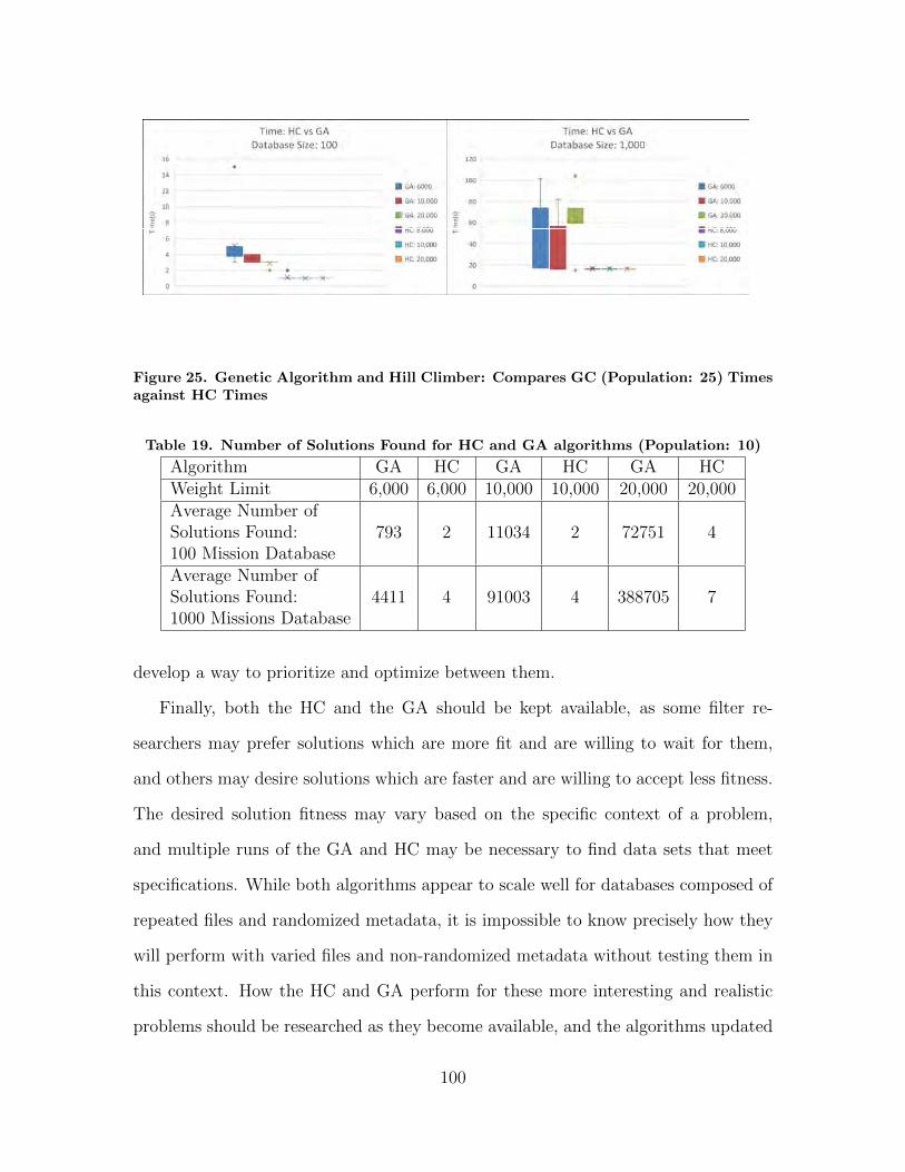
Figure 25. Genetic Algorithm and Hill Climber: Compares GC (Population: 25) Timesagainst HC Times
Table 19. Number of Solutions Found for HC and GA algorithms (Population: 10)
Algorithm GA HC GA HC GA HCWeight Limit 6,000 6,000 10,000 10,000 20,000 20,000Average Number ofSolutions Found:100 Mission Database
793 2 11034 2 72751 4
Average Number ofSolutions Found:1000 Missions Database
4411 4 91003 4 388705 7
develop a way to prioritize and optimize between them.
Finally, both the HC and the GA should be kept available, as some filter re-
searchers may prefer solutions which are more fit and are willing to wait for them,
and others may desire solutions which are faster and are willing to accept less fitness.
The desired solution fitness may vary based on the specific context of a problem,
and multiple runs of the GA and HC may be necessary to find data sets that meet
specifications. While both algorithms appear to scale well for databases composed of
repeated files and randomized metadata, it is impossible to know precisely how they
will perform with varied files and non-randomized metadata without testing them in
this context. How the HC and GA perform for these more interesting and realistic
problems should be researched as they become available, and the algorithms updated
100

as necessary.
101
V. Conclusion
This thesis presents three different relational database schemas based on the Scor-
pion Data Model format [7]. Each approach has common schemas for storing sensor
and non-sensor related metadata, and different schemas for storing SDM data. Ap-
proach 1 places all SDM data of a given type into a corresponding table. These
tables grow indefinitely as additional data is added. This approach limits the num-
ber of tables which must be created, but results with queries taking longer as the
tables grow larger. Approach 2 places SDM data into a table corresponding to both
data type and mission number, which limits their size. This will result in more ta-
bles, but helps speed up searches and with distributing the tables between nodes.
Approach 3 is a variation of Approach 1, except that tables are not made for the
IMU and OpticalCameraImage data types due to their frequency and size, and the
original data log is made available for download in the case that these tables were
queried. The need to download the original data log for all missions of interest make
queries against the IMU and OpticalCameraImage data types take longer, but speeds
up downloading the original log file. There are two test databases for each approach,
one with 100 missions and one with 1000 missions, for a total of six databases. These
numbers are selected based on the number of data logs that AFIT is estimated to
have, and to allow room for growth in the future.
The ANT center provided a set of questions which were used to build the SQL
queries to test the three approaches. There are three query categories in testing,
one where the SDM tables are queried (SDM Query Test), one where the original
file or a subset is downloaded (Download Test), and one where non-SDM data is
queried (Metadata Query Test). Each test is composed of multiple sub-tests, and
each sub-test was run 11 times for each of the six databases.
In all but two cases, Approach 3 outperforms the other two approaches for the
102

Download Test. Approach 1 and 2 outperform Approach 3 when the subset of the
downloaded file is small enough that it is quicker to reconstruct it using queries
to populate LCM events and write these events to a file, rather than downloading
and parsing the original file. Approaches 1 and 2 perform almost equally well, with
Approach 2 outperforming Approach 1 in most cases. This is more pronounced for the
larger databases, with Approach 2 typically being between 1 and 2 seconds faster than
Approach 1. Overall, Approach 3 has the strongest performance for the Download
Test, with both Approaches 1 and 2 having acceptable performances.
For the SDM Query Test, Approach 2 outperforms Approaches 1 and 3 in all
cases. For the Platform Dynamics Test, which consults the IMU tables for magnitude
of g’s experienced during the mission, Approach 2 performs a factor of 4 faster than
Approach 3, and an average of 11 minutes faster than Approach 1 for the 1000
mission databases. For the Satellite Type Test, which consults the GNSS table, the
three approaches perform equivalently well, with Approach 2 being approximately
200ms faster than the other two approaches. For the other three tests, Approach
2 on average was twice as fast or more than the other approaches. The difference
between Approaches 1 and 2 is due to the time it take to query the larger tables. This
difference all but disappears for the GNSS table, due to it only having 2 million rows
in the 1000 mission database, in comparison to 426 million rows in the IMU table.
The difference between Approach 2 and Approach 3 is due to Approach 3 having to
download and parse all 1000 log files when the IMU table is consulted. For the SDM
Query Test, Approach 3 performs prohibitively badly, and Approach 2 has the best
overall performance.
The tests for the non-SDM database tables (Metadata Query Test) demonstrate
that the proposed schema scales well from 100 data logs to 1000 data logs, completing
all but one query in under half a second even for the larger databases, and that
103

various databases containing randomized data perform similarly well using the same
underlying schema.
Once testing showed that Approach 2 had the best overall performance, the two
test databases were used with the Hill Climber algorithm and Genetic Algorithm for
Multi-Objective queries in the combined KP/SCP Problem Domain. This problem
domain allows researchers to use simple queries to return solutions to more complex
ones. The examples used with the GA and HC algorithm attempt to maximize the
number of recorded events that took place above 1000 meters, include at least one of a
set of sensor types and terrain types, and keep the total time of the returned missions
below a certain limit. Any queries could be used to replace those listed here and work
with the algorithms, as long as their returned answers met the correct formats.
The GA creates a population of 10, 25 or 50 solutions, and then uses stochastic
and deterministic processes to crossover and mutate these solutions, and then add
them back in to the population if their fitness is improved. The GA terminates if
a certain amount of time passes or if 100 iterations pass without a better solution
being found. The HC algorithm finds a single solution, and then swaps all 0’s and
1’s looking for a better solution.
Both of these algorithms returned correct solution sets that met the PD con-
straints, and were tested 10 times for each permutation and each database. These
queries demonstrated that the HC algorithm returned less-optimal solutions more
quickly, and the GA algorithm returned more-optimal solutions less quickly. The
population size did not make a noticeable difference for the returned value of the GA.
The next step is to implement the Approach 2 schema with AFIT’s set of data.
The first design decision is to determine the details of the database distribution, load
it with real data, and then offer it on a cloud service. Following this, AFIT students
should use it to enable their own research, and provide feedback for improvement.
104

The HC and GA should be incorporated as part of the user interface to help students
perform queries, and if desired queries are sufficiently complex they could be used to
facilitate additional research.
105

Appendix A. Full Database Schema
missionDescription
id INTEGER PK
startDate_UTC DATE
endDate_UTC DATE
organization TEXT
missionLocationStart TEXT
missionLocationEnd TEXT
platform TEXT
missionLength_Seconds BIGINT
dataFileSize BIGINT
PK_missionDescription
loopClosures
id TEXT PK
time INTEGER
latitude DOUBLE PRECISION
longitude DOUBLE PRECISION
missionDescription_id INTEGER FK
PK_loopClosures
wayPoints
id INTEGER PK
time INTEGER
latitude DOUBLE PRECISION
longitude DOUBLE PRECISION
missionDescription_id INTEGER FK
PK_wayPoints
altitudeSegments
id INTEGER PK
start_altitude INTEGER
end_altitude INTEGER
approximate_duration INTEGER
missionDescription_id INTEGER FK
PK_altitudeSegments
obscuration
obscuration TEXT PK
missionDescription_id INTEGER PK FK
PK_obscuration
precipitation
precipitation TEXT PK
intensity NUMERIC PK
missionDescription_id INTEGER PK FK
PK_precipitation
terrain
type TEXT PK
missionDescription_id INTEGER PK FK
PK_terrain
manuevers
id INTEGER PK
manuever TEXT
approximate_duration INTEGER
missionDescription_id INTEGER FK
PK_manuevers
skycover
skycover TEXT PK
missionDescription_id INTEGER PK FK
PK_skycover
unexpectedResults
unexpectedResults TEXT
id INTEGER FK
Figure 26. nonSensorMetadata
106

missionDescription
id INTEGER PK
startDate_UTC DATE
endDate_UTC DATE
organization TEXT
missionLocationStart TEXT
missionLocationEnd TEXT
platform TEXT
missionLength_Seconds BIGINT
dataFileSize BIGINT
PK_missionDescription
channelInfo
id INTEGER PK
channelName TEXT
channelUse TEXT
deviceID TEXT
truth BOOLEAN
missionDescription_id INTEGER FK
sensorInstallation_id INTEGER FK
PK_channelInfo
sensorModel
outage
id INTEGER PK
planned BOOLEAN
approximate_duration INTEGER
intermittent BOOLEAN
PK_outage
outage_channel
channel_id INTEGER FK
outage_id INTEGER FK
Figure 27. missionDescription and channelInfo
107

channelInfo
id INTEGER PK
channelName TEXT
channelUse TEXT
deviceID TEXT
truth BOOLEAN
missionDescription_id INTEGER FK
sensorInstallation_id INTEGER FK
PK_channelInfo
velocity3d
id INTEGER PK
timeStamp_arrival_second BIGINT
timeStamp_arrival_nsec INTEGER
timeStamp_valid_sec BIGINT
timeStamp_valid_nsec INTEGER
utime BIGINT
eventNumber BIGINT
seqNumber BIGINT
logByteOffset BIGINT
x DOUBLE PRECISION
y DOUBLE PRECISION
z DOUBLE PRECISION
covariance DOUBLE PRECISION
channel_id INTEGER FK
PK_velocity3d
velocity1d
id INTEGER PK
timeStamp_arrival_second BIGINT
timeStamp_arrival_nsec INTEGER
timeStamp_valid_sec BIGINT
timeStamp_valid_nsec INTEGER
utime BIGINT
eventNumber BIGINT
seqNumber BIGINT
logByteOffset BIGINT
x DOUBLE PRECISION
variance DOUBLE PRECISION
channel_id INTEGER FK
PK_velocity1d
speed
id INTEGER PK
timeStamp_arrival_second BIGINT
timeStamp_arrival_nsec INTEGER
timeStamp_valid_sec BIGINT
timeStamp_valid_nsec INTEGER
utime BIGINT
eventNumber BIGINT
seqNumber BIGINT
logByteOffset BIGINT
speed DOUBLE PRECISION
variance DOUBLE PRECISION
channel_id INTEGER FK
PK_speed
altitude
id INTEGER PK
timeStamp_arrival_second BIGINT
timeStamp_arrival_nsec INTEGER
timeStamp_valid_sec BIGINT
timeStamp_valid_nsec INTEGER
utime BIGINT
eventNumber BIGINT
seqNumber BIGINT
logByteOffset BIGINT
altitude DOUBLE PRECISION
variance DOUBLE PRECISION
channel_id INTEGER FK
PK_altitude
geodeticposition3d
id INTEGER PK
timeStamp_arrival_second BIGINT
timeStamp_arrival_nsec INTEGER
timeStamp_valid_sec BIGINT
timeStamp_valid_nsec INTEGER
utime BIGINT
eventNumber BIGINT
seqNumber BIGINT
logByteOffset BIGINT
latitude DOUBLE PRECISION
longitude DOUBLE PRECISION
altitude DOUBLE PRECISION
covariance DOUBLE PRECISION
channel_id INTEGER FK
PK_geodeticposition3d
threeaxismagnetometer
id INTEGER PK
timeStamp_arrival_second BIGINT
timeStamp_arrival_nsec INTEGER
timeStamp_valid_sec BIGINT
timeStamp_valid_nsec INTEGER
utime BIGINT
eventNumber BIGINT
seqNumber BIGINT
logByteOffset BIGINT
field DOUBLE PRECISION
covariance DOUBLE PRECISION
channel_id INTEGER FK
PK_threeaxismagnetometer
positionvelocityattitude
id INTEGER PK
timeStamp_arrival_second BIGINT
timeStamp_arrival_nsec INTEGER
timeStamp_valid_sec BIGINT
timeStamp_valid_nsec INTEGER
utime BIGINT
eventNumber BIGINT
seqNumber BIGINT
logByteOffset BIGINT
latitude DOUBLE PRECISION
longitude DOUBLE PRECISION
altitude DOUBLE PRECISION
velocity DOUBLE PRECISION
attitude DOUBLE PRECISION
covariance DOUBLE PRECISION
channel_id INTEGER FK
PK_positionvelocityattitude
opticalcameraimage
id INTEGER PK
timeStamp_arrival_second BIGINT
timeStamp_arrival_nsec INTEGER
timeStamp_valid_sec BIGINT
timeStamp_valid_nsec INTEGER
utime BIGINT
eventNumber BIGINT
seqNumber BIGINT
logByteOffset BIGINT
encoding DOUBLE PRECISION
height DOUBLE PRECISION
width INTEGER
num_channels INTEGER
array_length INTEGER
data BYTEA
channel_id INTEGER FK
PK_opticalcameraimage
imu
id INTEGER PK
timeStamp_arrival_second BIGINT
timeStamp_arrival_nsec INTEGER
timeStamp_valid_sec BIGINT
timeStamp_valid_nsec INTEGER
utime BIGINT
eventNumber BIGINT
seqNumber BIGINT
logByteOffset BIGINT
delta_v DOUBLE PRECISION
delta_theta DOUBLE PRECISION
channel_id INTEGER FK
PK_imu
gpsephemeris
id INTEGER PK
timeStamp_arrival_second BIGINT
timeStamp_arrival_nsec INTEGER
timeStamp_valid_sec BIGINT
timeStamp_valid_nsec INTEGER
utime BIGINT
eventNumber BIGINT
seqNumber BIGINT
logByteOffset BIGINT
prn INTEGER
wn_t_oc INTEGER
t_oc DOUBLE PRECISION
t_gd DOUBLE PRECISION
af_0 DOUBLE PRECISION
af_1 DOUBLE PRECISION
af_2 DOUBLE PRECISION
m_0 DOUBLE PRECISION
delta_n DOUBLE PRECISION
e DOUBLE PRECISION
sqrt_a DOUBLE PRECISION
omega_0 DOUBLE PRECISION
i_0 DOUBLE PRECISION
i_dot DOUBLE PRECISION
omega DOUBLE PRECISION
omega_dot DOUBLE PRECISION
c_uc DOUBLE PRECISION
c_us DOUBLE PRECISION
c_rc DOUBLE PRECISION
c_rs DOUBLE PRECISION
c_ic DOUBLE PRECISION
c_is DOUBLE PRECISION
wn_t_oe INTEGER
t_oe DOUBLE PRECISION
channel_id INTEGER FK
PK_gpsephemeris
gnss
id INTEGER PK
timeStamp_arrival_second BIGINT
timeStamp_arrival_nsec INTEGER
timeStamp_valid_sec BIGINT
timeStamp_valid_nsec INTEGER
utime BIGINT
eventNumber BIGINT
seqNumber BIGINT
logByteOffset BIGINT
week_number DOUBLE PRECISION
seconds_of_week DOUBLE PRECISION
time_system TEXT
epoch_flag INTEGER
num_satellites INTEGER
num_measurements INTEGER
obs_prn INTEGER
satellite_system TEXT
type TEXT
band TEXT
attribute TEXT
observation DOUBLE PRECISION
LLI INTEGER
signal_strength INTEGER
lock_count INTEGER
channel_id INTEGER FK
PK_gnss
sensorRegistrationAck
id INTEGER PK
utime BIGINT
eventNumber BIGINT
logByteOffset BIGINT
registered BOOLEAN
sensorUID TEXT
channel_id INTEGER FK
PK_sensorRegistrationAck
non_SDM_Message
id INTEGER PK
utime BIGINT
eventNumber BIGINT
logByteOffset BIGINT
data BYTEA
channel_id INTEGER FK
PK_non_SDM_Message
Figure 28. SDM Tables
108
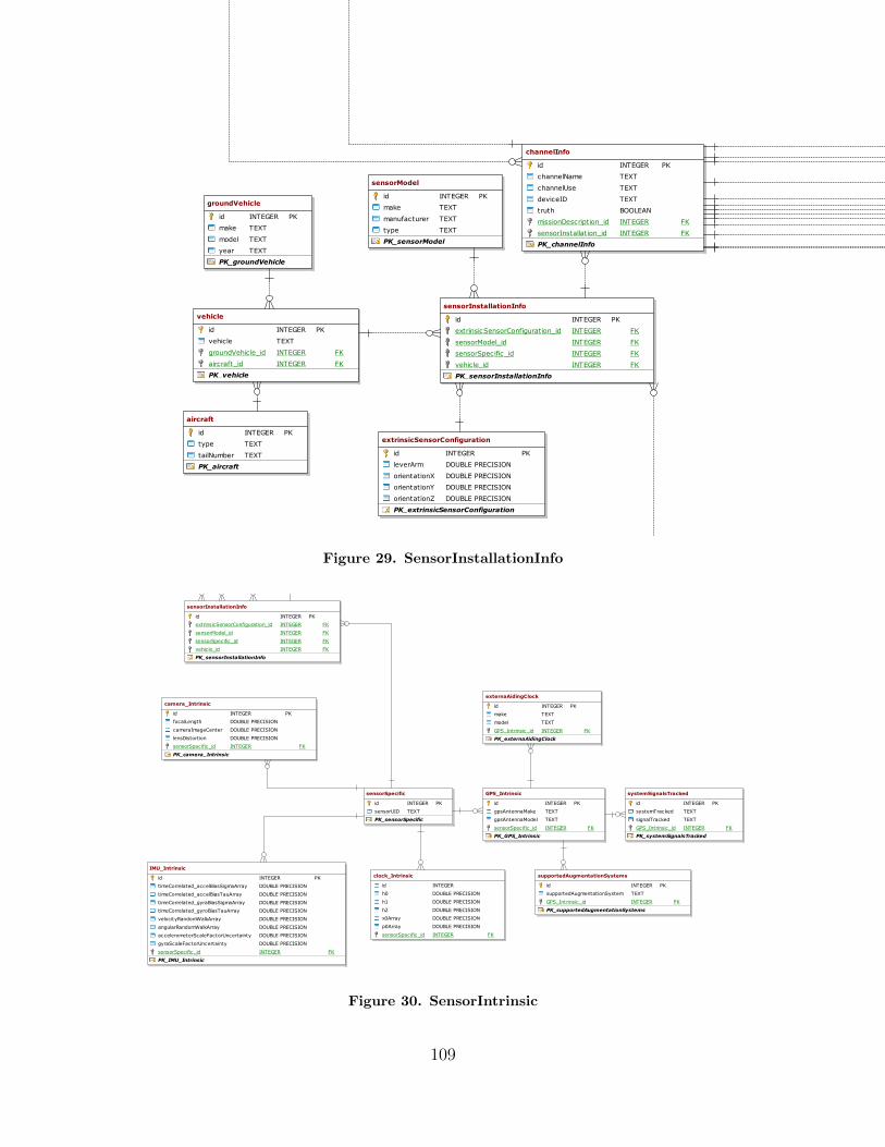
channelInfo
id INTEGER PK
channelName TEXT
channelUse TEXT
deviceID TEXT
truth BOOLEAN
missionDescription_id INTEGER FK
sensorInstallation_id INTEGER FK
PK_channelInfo
sensorModel
id INTEGER PK
make TEXT
manufacturer TEXT
type TEXT
PK_sensorModel
sensorInstallationInfo
id INTEGER PK
extrinsicSensorConfiguration_id INTEGER FK
sensorModel_id INTEGER FK
sensorSpecific_id INTEGER FK
vehicle_id INTEGER FK
PK_sensorInstallationInfo
extrinsicSensorConfiguration
id INTEGER PK
leverArm DOUBLE PRECISION
orientationX DOUBLE PRECISION
orientationY DOUBLE PRECISION
orientationZ DOUBLE PRECISION
PK_extrinsicSensorConfiguration
aircraft
id INTEGER PK
type TEXT
tailNumber TEXT
PK_aircraft
groundVehicle
id INTEGER PK
make TEXT
model TEXT
year TEXT
PK_groundVehicle
vehicle
id INTEGER PK
vehicle TEXT
groundVehicle_id INTEGER FK
aircraft_id INTEGER FK
PK_vehicle
Figure 29. SensorInstallationInfo
sensorInstallationInfo
id INTEGER PK
extrinsicSensorConfiguration_id INTEGER FK
sensorModel_id INTEGER FK
sensorSpecific_id INTEGER FK
vehicle_id INTEGER FK
PK_sensorInstallationInfo
sensorSpecific
id INTEGER PK
sensorUID TEXT
PK_sensorSpecific
IMU_Intrinsic
id INTEGER PK
timeCorrelated_accelBiasSigmaArray DOUBLE PRECISION
timeCorrelated_accelBiasTauArray DOUBLE PRECISION
timeCorrelated_gyraBiasSigmaArray DOUBLE PRECISION
timeCorrelated_gyroBiasTauArray DOUBLE PRECISION
velocityRandomWalkArray DOUBLE PRECISION
angularRandomWalkArray DOUBLE PRECISION
accelerometerScaleFactorUncertainty DOUBLE PRECISION
gyraScaleFactorUncertainty DOUBLE PRECISION
sensorSpecific_id INTEGER FK
PK_IMU_Intrinsic
clock_Intrinsic
id INTEGER
h0 DOUBLE PRECISION
h1 DOUBLE PRECISION
h2 DOUBLE PRECISION
x0Array DOUBLE PRECISION
p0Array DOUBLE PRECISION
sensorSpecific_id INTEGER FK
camera_Intrinsic
id INTEGER PK
focalLength DOUBLE PRECISION
cameraImageCenter DOUBLE PRECISION
lensDistortion DOUBLE PRECISION
sensorSpecific_id INTEGER FK
PK_camera_Intrinsic
GPS_Intrinsic
id INTEGER PK
gpsAntennaMake TEXT
gpsAntennaModel TEXT
sensorSpecific_id INTEGER FK
PK_GPS_Intrinsic
externaAidingClock
id INTEGER PK
make TEXT
model TEXT
GPS_Intrinsic_id INTEGER FK
PK_externaAidingClock
systemSignalsTracked
id INTEGER PK
systemTracked TEXT
signalTracked TEXT
GPS_Intrinsic_id INTEGER FK
PK_systemSignalsTracked
supportedAugmentationSystems
id INTEGER PK
supportedAugmentationSystem TEXT
GPS_Intrinsic_id INTEGER FK
PK_supportedAugmentationSystems
Figure 30. SensorIntrinsic
109

missionDescription
id INTEGER PK
startDate_UTC DATE
endDate_UTC DATE
organization TEXT
missionLocationStart TEXT
missionLocationEnd TEXT
platform TEXT
missionLength_Seconds BIGINT
dataFileSize BIGINT
PK_missionDescription
channelInfo
id INTEGER PK
channelName TEXT
channelUse TEXT
deviceID TEXT
truth BOOLEAN
missionDescription_id INTEGER FK
sensorInstallation_id INTEGER FK
PK_channelInfo
sensorModel
id INTEGER PK
make TEXT
manufacturer TEXT
PK_sensorModel
sensorType
id INTEGER PK
type TEXT
model_id INTEGER FK
sensorInstallation
id INTEGER PK
extrinsicSensorConfiguration_id INTEGER FK
sensorModel_id INTEGER FK
sensorSpecific_id INTEGER FK
PK_sensorInstallation
FK_channelInfo_missionDescription
FK_sensorType_sensorModel
sensorSpecific
id INTEGER PK
sensorUID TEXT
PK_sensorSpecific
FK_sensorInstallation_sensorModel
FK_sensorInstallation_sensorSpec ific
outage
id INTEGER PK
planned BOOLEAN
approximate_duration INTEGER
intermittent BOOLEAN
PK_outage
outage_track
channel_id INTEGER FK
outage_id INTEGER FK
extrinsicSensorConfiguration
id INTEGER PK
leverArm DOUBLE PRECISION
orientationX DOUBLE PRECISION
orientationY DOUBLE PRECISION
orientationZ DOUBLE PRECISION
PK_extrinsicSensorConfiguration
FK_sensorInstallation_extrinsicSensorConfiguration
FK_outage_track_outage
FK_outage_track_channelInfo
IMU_Intrinsic
id INTEGER PK
timeCorrelated_accelBiasSigmaArray DOUBLE PRECISION
timeCorrelated_accelBiasTauArray DOUBLE PRECISION
timeCorrelated_gyraBiasSigmaArray DOUBLE PRECISION
timeCorrelated_gyroBiasTauArray DOUBLE PRECISION
velocityRandomWalkArray DOUBLE PRECISION
angularRandomWalkArray DOUBLE PRECISION
accelerometerScaleFactorUncertainty DOUBLE PRECISION
gyraScaleFactorUncertainty DOUBLE PRECISION
sensorSpecific_id INTEGER FK
PK_IMU_Intrinsic
FK_IMU_Intrinsic_sensorSpec ific
clock_Intrinsic
id INTEGER
h0 DOUBLE PRECISION
h1 DOUBLE PRECISION
h2 DOUBLE PRECISION
x0Array DOUBLE PRECISION
p0Array DOUBLE PRECISION
sensorSpecific_id INTEGER FK
FK_clock_Intrinsic_sensorSpecific
camera_Intrinsic
id INTEGER PK
focalLength DOUBLE PRECISION
cameraImageCenter DOUBLE PRECISION
lensDistortion DOUBLE PRECISION
sensorSpecific_id INTEGER FK
PK_camera_Intrinsic
FK_camera_Intrinsic_sensorSpec ific
GPS_Intrinsic
id INTEGER PK
gpsAntennaMake TEXT
gpsAntennaModel TEXT
sensorSpecific_id INTEGER FK
PK_GPS_Intrinsic
FK_GPS_Intrinsic_sensorSpec ific
externaAidingClock
id INTEGER PK
make TEXT
model TEXT
GPS_Intrinsic_id INTEGER FK
PK_externaAidingClock
systemSignalsTracked
id INTEGER PK
systemTracked TEXT
signalTracked TEXT
GPS_Intrinsic_id INTEGER FK
PK_systemSignalsTracked
supportedAugmentationSystems
id INTEGER PK
supportedAugmentationSystem TEXT
GPS_Intrinsic_id INTEGER FK
PK_supportedAugmentationSystems
FK_externaAidingClock_GPS_Intrinsic
FK_systemSignalsTracked_GPS_Intrinsic
FK_supportedAugmentationSystems_GPS_Intrinsic
FK_channelInfo_sensorInstallation
velocity3d
id INTEGER PK
timeStamp_arrival_second BIGINT
timeStamp_arrival_nsec INTEGER
timeStamp_valid_sec BIGINT
timeStamp_valid_nsec INTEGER
utime BIGINT
eventNumber BIGINT
seqNumber BIGINT
logByteOffset BIGINT
x DOUBLE PRECISION
y DOUBLE PRECISION
z DOUBLE PRECISION
covariance DOUBLE PRECISION
channel_id INTEGER FK
PK_velocity3d
velocity1d
id INTEGER PK
timeStamp_arrival_second BIGINT
timeStamp_arrival_nsec INTEGER
timeStamp_valid_sec BIGINT
timeStamp_valid_nsec INTEGER
utime BIGINT
eventNumber BIGINT
seqNumber BIGINT
logByteOffset BIGINT
x DOUBLE PRECISION
variance DOUBLE PRECISION
channel_id INTEGER FK
PK_velocity1d
speed
id INTEGER PK
timeStamp_arrival_second BIGINT
timeStamp_arrival_nsec INTEGER
timeStamp_valid_sec BIGINT
timeStamp_valid_nsec INTEGER
utime BIGINT
eventNumber BIGINT
seqNumber BIGINT
logByteOffset BIGINT
speed DOUBLE PRECISION
variance DOUBLE PRECISION
channel_id INTEGER FK
PK_speed
altitude
id INTEGER PK
timeStamp_arrival_second BIGINT
timeStamp_arrival_nsec INTEGER
timeStamp_valid_sec BIGINT
timeStamp_valid_nsec INTEGER
utime BIGINT
eventNumber BIGINT
seqNumber BIGINT
logByteOffset BIGINT
altitude DOUBLE PRECISION
variance DOUBLE PRECISION
channel_id INTEGER FK
PK_altitude
geodeticposition3d
id INTEGER PK
timeStamp_arrival_second BIGINT
timeStamp_arrival_nsec INTEGER
timeStamp_valid_sec BIGINT
timeStamp_valid_nsec INTEGER
utime BIGINT
eventNumber BIGINT
seqNumber BIGINT
logByteOffset BIGINT
latitude DOUBLE PRECISION
longitude DOUBLE PRECISION
altitude DOUBLE PRECISION
covariance DOUBLE PRECISION
channel_id INTEGER FK
PK_geodeticposition3d
threeaxismagnetometer
id INTEGER PK
timeStamp_arrival_second BIGINT
timeStamp_arrival_nsec INTEGER
timeStamp_valid_sec BIGINT
timeStamp_valid_nsec INTEGER
utime BIGINT
eventNumber BIGINT
seqNumber BIGINT
logByteOffset BIGINT
field DOUBLE PRECISION
covariance DOUBLE PRECISION
channel_id INTEGER FK
PK_threeaxismagnetometer
positionvelocityattitude
id INTEGER PK
timeStamp_arrival_second BIGINT
timeStamp_arrival_nsec INTEGER
timeStamp_valid_sec BIGINT
timeStamp_valid_nsec INTEGER
utime BIGINT
eventNumber BIGINT
seqNumber BIGINT
logByteOffset BIGINT
latitude DOUBLE PRECISION
longitude DOUBLE PRECISION
altitude DOUBLE PRECISION
velocity DOUBLE PRECISION
attitude DOUBLE PRECISION
covariance DOUBLE PRECISION
channel_id INTEGER FK
PK_positionvelocityattitude
opticalcameraimage
id INTEGER PK
timeStamp_arrival_second BIGINT
timeStamp_arrival_nsec INTEGER
timeStamp_valid_sec BIGINT
timeStamp_valid_nsec INTEGER
utime BIGINT
eventNumber BIGINT
seqNumber BIGINT
logByteOffset BIGINT
encoding DOUBLE PRECISION
height DOUBLE PRECISION
width INTEGER
num_channels INTEGER
array_length INTEGER
data BYTEA
channel_id INTEGER FK
PK_opticalcameraimage
imu
id INTEGER PK
timeStamp_arrival_second BIGINT
timeStamp_arrival_nsec INTEGER
timeStamp_valid_sec BIGINT
timeStamp_valid_nsec INTEGER
utime BIGINT
eventNumber BIGINT
seqNumber BIGINT
logByteOffset BIGINT
delta_v DOUBLE PRECISION
delta_theta DOUBLE PRECISION
channel_id INTEGER FK
PK_imu
gnss
id INTEGER PK
timeStamp_arrival_second BIGINT
timeStamp_arrival_nsec INTEGER
timeStamp_valid_sec BIGINT
timeStamp_valid_nsec INTEGER
utime BIGINT
eventNumber BIGINT
seqNumber BIGINT
logByteOffset BIGINT
week_number DOUBLE PRECISION
seconds_of_week DOUBLE PRECISION
time_system TEXT
epoch_flag INTEGER
num_satellites INTEGER
num_measurements INTEGER
obs_prn INTEGER
satellite_system TEXT
type TEXT
band TEXT
attribute TEXT
observation DOUBLE PRECISION
LLI INTEGER
signal_strength INTEGER
lock_count INTEGER
channel_id INTEGER FK
PK_gnss
gpsephemeris
id INTEGER PK
timeStamp_arrival_second BIGINT
timeStamp_arrival_nsec INTEGER
timeStamp_valid_sec BIGINT
timeStamp_valid_nsec INTEGER
utime BIGINT
eventNumber BIGINT
seqNumber BIGINT
logByteOffset BIGINT
prn INTEGER
wn_t_oc INTEGER
t_oc DOUBLE PRECISION
t_gd DOUBLE PRECISION
af_0 DOUBLE PRECISION
af_1 DOUBLE PRECISION
af_2 DOUBLE PRECISION
m_0 DOUBLE PRECISION
delta_n DOUBLE PRECISION
e DOUBLE PRECISION
sqrt_a DOUBLE PRECISION
omega_0 DOUBLE PRECISION
i_0 DOUBLE PRECISION
i_dot DOUBLE PRECISION
omega DOUBLE PRECISION
omega_dot DOUBLE PRECISION
c_uc DOUBLE PRECISION
c_us DOUBLE PRECISION
c_rc DOUBLE PRECISION
c_rs DOUBLE PRECISION
c_ic DOUBLE PRECISION
c_is DOUBLE PRECISION
wn_t_oe INTEGER
t_oe DOUBLE PRECISION
channel_id INTEGER FK
PK_gpsephemeris
sensorRegistrationAck
id INTEGER PK
utime BIGINT
eventNumber BIGINT
logByteOffset BIGINT
registered BOOLEAN
sensorUID TEXT
channel_id INTEGER FK
PK_sensorRegistrationAck
non_SDM_Message
id INTEGER PK
utime BIGINT
eventNumber BIGINT
logByteOffset BIGINT
data BYTEA
channel_id INTEGER FK
PK_non_SDM_Message
FK_veloc ity3d_channelInfo
FK_veloc ity1d_channelInfo
FK_speed_channelInfo
FK_altitude_channelInfo
FK_geodeticposition3d_channelInfo
FK_threeaxismagnetometer_channelInfo
FK_imu_channelInfo
FK_gpsephemeris_channelInfo
FK_sensorRegistrationAck_channelInfo
FK_non_SDM_Message_channelInfo
FK_positionveloc ityattitude_channelInfoFK_opticalcameraimage_channelInfo
FK_gnss_channelInfo
loopClosures
id TEXT PK
time INTEGER
latitude DOUBLE PRECISION
longitude DOUBLE PRECISION
missionDescription_id INTEGER FK
PK_loopClosures
wayPoints
id INTEGER PK
time INTEGER
latitude DOUBLE PRECISION
longitude DOUBLE PRECISION
missionDescription_id INTEGER FK
PK_wayPoints
altitudeSegments
id INTEGER PK
start_altitude INTEGER
end_altitude INTEGER
approximate_duration INTEGER
missionDescription_id INTEGER FK
PK_altitudeSegments
obscuration
obscuration TEXT PK
missionDescription_id INTEGER PK FK
PK_obscuration
precipitation
precipitation TEXT PK
intensity NUMERIC PK
missionDescription_id INTEGER PK FK
PK_precipitation
terrain
type TEXT PK
missionDescription_id INTEGER PK FK
PK_terrain
aircraft_missionDescription
missionDescription_id INTEGER
aircraft_id INTEGER
missionDescription_id1 INTEGER FK
aircraft_id1 INTEGER FK
aircraft
id INTEGER PK
type TEXT
tailNumber TEXT
PK_aircraft
groundVehicle_missionDescription
groundVehic le_id INTEGER FK
missionDescription_id INTEGER FK
groundVehicle
id NUMERIC PK
make TEXT
model TEXT
year TEXT
PK_groundVehicle
manuevers
id INTEGER PK
manuever TEXT
approximate_duration NUMERIC
missionDescription_id INTEGER FK
PK_manuevers
FK_aircraft_missionDescription_aircraft
FK_aircraft_missionDescription_missionDescription
FK_groundVehicle_missionDescription_groundVehic le
FK_groundVehicle_missionDescription_missionDescription
FK_terrain_missionDescription
FK_prec ipitation_missionDescription
FK_obscuration_missionDescription
skycover
skycover TEXT PK
missionDescription_id INTEGER PK FK
PK_skycover
FK_skycover_missionDescription
FK_manuevers_missionDescription
FK_altitudeSegments_missionDescription
FK_wayPoints_missionDescription
FK_loopClosures_missionDescription
unexpectedResults
unexpectedResults TEXT
id INTEGER FK
FK_unexpectedResults_missionDescription
Figure 31. Full Database Schema
110

Appendix B. Tester Questionnaire
The Tester Questionnaire is designed for testers to complete immediately after
testing in under five minutes. It captures data of interest from the test to be recorded
in the relational database described in this thesis. When formatted and printed it
fits on a single piece of paper front and back.
Instructions:
1. Please keep answers as short as possible
2. Leave answers blank if unknown
Date:
Vehicle Type:
Vehicle Tail Number:
Testers:
Table 20. Recordings for loop closures
Loop ClosuresTime Latitude Longitude
Table 21. Recordings for Way Points
Way PointsTime Latitude Longitude
111

Table 22. Maneuvers
Maneuvers (Figure 8, Figure S, Circle, etc.Maneuver Approximate Duration
Table 23. Altitude Segments
Altitude Segments (ascending, descending, unchanging, etc.)Start Altitude End Altitude Approximate Duration
Table 24. Precipitation
Precipitation (leave unmarked if none)Light Moderate Heavy
RainSnowHail
Other conditions (Cloudy, Sunny?):
If you have an EO/IR sensor facing the ground, please fill out obscuration and terrain
sections:
Obscuration (Fog, Mist, Smoke, Dust?):
112

Terrain Type (Hills, Flat, Canopy, Water, Desert?):
Table 25. Sensor Outages
Sensor Outages
Sensor Type Model LCM Channel Planned?ApproximateDuration
Intermittent?
Table 26. GPS Outages
GPS OutagesSimulated or Actual? Planned or Unplanned? Approximate Duration Intermittent?
Table 27. System Malfunctions and Unexpected Results
System Malfunctions and Unexpected ResultsDescription Approximate Duration
113

Appendix C. Database Test Results
Appendix C provides the raw test data associated with the ION/PLANS confer-
ence paper.
114
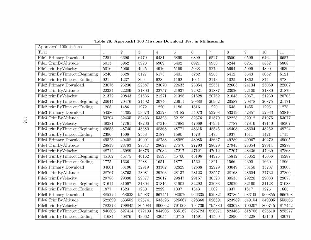
Table 28. Approach1 100 Missions Download Test in Milliseconds
Approach1 100missions
Trial 1 2 3 4 5 6 7 8 9 10 11
File1 Primary Download 7251 6696 6479 6481 6899 6899 6527 6550 6599 6464 6657
File1 TrimByAltitude 6013 5962 5923 5909 6402 6921 5950 6244 6251 5882 5808
File1 trimByVelocity 5016 5066 4925 4916 5169 5038 5279 5694 5099 4890 4939
File1 trimByTime cutBeginning 5240 5328 5127 5173 5401 5282 5288 6412 5343 5082 5121
File1 trimByTime cutEnding 921 1237 899 928 1192 1041 2113 1025 1862 874 878
File2 Primary Download 23076 23236 22887 23070 22633 23054 22551 22605 24134 23059 22807
File2 TrimByAltitude 22334 22289 21800 22757 21937 22921 21887 23026 22100 21880 21879
File2 trimByVelocity 21372 20843 21636 21271 21398 21528 20762 21045 20671 21230 20705
File2 trimByTime cutBeginning 20644 20476 21492 20746 20611 20388 20962 20587 20878 20875 21171
File2 trimByTime cutEnding 1208 1486 1972 1220 1186 1816 1220 1548 1455 1295 1275
File3 Primary Download 54286 54305 53673 53528 53182 54073 53208 53219 52857 52933 53810
File3 TrimByAltitude 53204 52435 52433 53325 52199 52576 51870 52225 52912 51975 53077
File3 trimByVelocity 49281 47761 48206 47316 47983 47669 47931 47787 47816 47140 48307
File3 trimByTime cutBeginning 49653 48740 48680 48368 48771 48315 48545 48408 48604 48252 49724
File3 trimByTime cutEnding 2396 1508 2558 2187 1590 1578 1473 1937 1511 1421 1715
File4 Primary Download 49523 49408 49091 48788 48989 48985 48637 49289 49067 49272 49005
File4 TrimByAltitude 28839 28783 27547 28628 27570 27793 28629 27945 28054 27914 28278
File4 trimByVelocity 48712 46989 46876 47082 47217 47121 47012 47207 48436 47939 47868
File4 trimByTime cutBeginning 45102 45775 46162 45593 45700 45196 44975 45812 45052 45056 45287
File4 trimByTime cutEnding 1775 1636 2288 1651 1877 1562 1821 1566 2390 1660 1896
File5 Primary Download 34061 33196 32919 33302 32829 32638 32929 33049 33150 33237 33008
File5 TrimByAltitude 28767 28763 28081 29203 28137 28123 28557 28168 28604 27732 27860
File5 trimByVelocity 29786 29390 29377 29617 29847 29157 30323 30535 29220 29083 29075
File5 trimByTime cutBeginning 31614 31097 31304 31816 31902 32292 32033 32029 32160 31128 31083
File5 trimByTime cutEnding 1877 1323 1260 2229 1337 1343 1502 1337 1817 1275 1665
File6 Primary Download 885226 958023 959831 967451 980076 966335 929821 937865 983100 960855 966798
File6 TrimByAltitude 522699 533552 526741 533526 525667 528368 526891 523982 549154 549005 555565
File6 trimByVelocity 782373 799845 805984 800062 791063 794739 795880 803028 790207 800745 817442
File6 trimByTime cutBeginning 840805 827414 872103 844905 835162 826723 826971 823463 818708 826610 825277
File6 trimByTime cutEnding 41684 40876 43062 43054 40712 41591 41569 42890 44228 43140 42077
115

Table 29. Approach2 100 Missions Download Test in Milliseconds
Approach2 100missions
Trial 1 2 3 4 5 6 7 8 9 10 11
File1 Primary Download 6412 6450 6411 6536 6450 6440 6367 6457 6402 6362 6443
File1 TrimByAltitude 5834 5826 5852 5812 5809 5807 5845 5783 5818 5835 5792
File1 trimByVelocity 4815 4817 4878 4885 4889 4851 4853 4806 4875 4853 4846
File1 trimByTime cutBeginning 5357 5788 5502 5576 5693 5279 5282 5708 5247 5356 5205
File1 trimByTime cutEnding 1232 1096 2093 1488 2083 1266 990 1741 1514 1357 1946
File2 Primary Download 22387 22209 22318 22391 22323 22417 22463 22543 22291 22257 22202
File2 TrimByAltitude 21555 21757 21906 21607 21626 21375 21386 21404 21434 21470 21323
File2 trimByVelocity 20463 20506 20393 20401 20291 20496 20676 20544 20406 20325 20466
File2 trimByTime cutBeginning 20479 20051 20705 20720 20774 21095 20603 20448 21176 20494 20400
File2 trimByTime cutEnding 1525 2317 1473 1492 1381 1582 2342 1291 1501 1483 1320
File3 Primary Download 52517 53382 52946 53025 52556 52781 52516 52525 52588 52555 53177
File3 TrimByAltitude 51670 51230 53310 51333 51546 51391 51401 51186 51132 51463 51243
File3 trimByVelocity 47051 47175 47093 47082 47143 46886 47019 46888 47013 47044 46909
File3 trimByTime cutBeginning 49102 48319 48061 48526 48589 48330 47912 47905 48406 48181 47565
File3 trimByTime cutEnding 2786 2459 1523 1825 1863 1554 2262 2041 1868 1760 1525
File4 Primary Download 48301 48449 48344 49011 48333 48966 48727 48667 48462 48426 48143
File4 TrimByAltitude 27730 27665 27687 27820 27527 27575 27768 27469 27287 27411 27715
File4 trimByVelocity 47031 46542 46721 46781 47709 46800 46626 48156 48076 46831 47129
File4 trimByTime cutBeginning 44829 44918 44392 44805 44716 44891 44907 45219 45005 44684 45247
File4 trimByTime cutEnding 2292 1879 1644 1625 1584 1943 1650 2844 2284 1935 1684
File5 Primary Download 32914 32534 32754 32849 32406 32601 32792 32744 33070 32730 32910
File5 TrimByAltitude 27759 27680 27630 27701 27438 27346 27634 27534 27650 27202 27789
File5 trimByVelocity 29050 28943 28739 29026 28784 28921 29313 29158 29172 28788 29017
File5 trimByTime cutBeginning 30701 30809 31391 31060 31506 30904 30719 31194 30947 31590 30672
File5 trimByTime cutEnding 1636 1372 2659 1833 2551 1883 1745 1734 1831 2182 1389
File6 Primary Download 937514 946676 945481 951807 949381 945337 942822 958700 963268 955885 954274
File6 TrimByAltitude 529335 518194 517359 536222 540111 543750 536315 537412 542968 543102 539398
File6 trimByVelocity 792029 809202 774991 782501 781273 788009 776597 785413 781905 791396 787424
File6 trimByTime cutBeginning 833252 847842 811126 808748 814748 809813 810243 815209 810383 810804 819083
File6 trimByTime cutEnding 43267 45106 44664 43813 44397 43168 43089 44016 44521 43806 43723
116
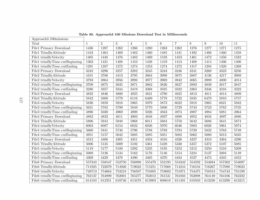
Table 30. Approach3 100 Missions Download Test in Milliseconds
Approach3 100missions
Trial 1 2 3 4 5 6 7 8 9 10 11
File1 Primary Download 1436 1287 1262 1266 1280 1263 1262 1276 1277 1271 1275
File1 TrimByAltitude 1443 1464 1469 1482 1460 1485 1441 1492 1466 1460 1458
File1 trimByVelocity 1405 1448 1476 1482 1469 1533 1453 1461 1472 1456 1582
File1 trimByTime cutBeginning 1363 1431 1408 1410 1438 1419 1413 1408 1414 1406 1406
File1 trimByTime cutEnding 1291 1287 1272 1274 1253 1274 1272 1317 1294 1320 1269
File2 Primary Download 3242 3296 3257 3282 3245 3243 3246 3241 3269 3323 3256
File2 TrimByAltitude 4101 3786 4413 3795 3864 3998 3875 3887 4136 4217 3989
File2 trimByVelocity 3793 3864 3956 3993 3977 3969 3942 4065 3989 4000 4014
File2 trimByTime cutBeginning 3709 3875 3835 3871 3862 3826 3827 3893 3839 3817 3847
File2 trimByTime cutEnding 3286 3357 3344 3419 3368 3325 3332 3363 3346 3316 3322
File3 Primary Download 4832 4846 4800 4825 4821 4790 4825 4813 4811 4814 4809
File3 TrimByAltitude 5842 5800 5779 6116 6469 5778 5732 5835 6479 5910 5757
File3 trimByVelocity 5830 5859 5916 5965 5979 5873 6022 5918 5965 6021 5942
File3 trimByTime cutBeginning 5621 5782 5799 5849 5770 5800 5729 5743 5723 5782 5735
File3 trimByTime cutEnding 4896 5030 4969 4998 5026 4943 4974 4987 4984 5081 4964
File4 Primary Download 4882 4833 4811 4903 4848 4937 4898 4952 4834 4897 4886
File4 TrimByAltitude 5806 5944 5948 5968 6011 5684 5750 5642 5686 5641 5874
File4 trimByVelocity 6063 6087 6154 6022 6026 5970 6046 5983 6026 5961 5974
File4 trimByTime cutBeginning 5660 5841 5746 5796 5788 5793 5794 5739 5832 5763 5749
File4 trimByTime cutEnding 4951 5157 5042 5085 5085 5051 5082 5062 5080 5013 5035
File5 Primary Download 4312 4406 4305 4351 4334 4316 4326 4327 4310 4364 4296
File5 TrimByAltitude 5006 5135 5009 5102 5361 5428 5330 5357 5372 5107 5085
File5 trimByVelocity 5119 5177 5180 5292 5235 5195 5252 5212 5250 5216 5209
File5 trimByTime cutBeginning 5069 5126 5134 5162 5176 5146 5154 5224 5137 5094 5149
File5 trimByTime cutEnding 4369 4429 4478 4490 4465 4370 4434 4537 4474 4345 4452
File6 Primary Download 557343 558547 552750 556998 555479 552195 554342 554592 554684 557302 554697
File6 TrimByAltitude 711925 722079 714926 719022 715251 717668 714244 716104 716267 717080 719023
File6 trimByVelocity 749713 754664 753218 756507 755805 753602 751971 754475 758313 754743 755199
File6 trimByTime cutBeginning 762137 764899 762001 765277 762012 761531 761050 763898 764149 764106 762222
File6 trimByTime cutEnding 614183 612351 610746 613478 613903 608618 611491 610503 613230 613290 613215
117

Table 31. Approach1 1000 Missions Download Test in Milliseconds
Approach1 1000missions
Trial 1 2 3 4 5 6 7 8 9 10 11
File1 Primary Download 8203 7739 7545 7338 7471 7401 7342 7210 7415 8304 7719
File1 TrimByAltitude 7029 7261 6671 6898 7173 7542 7064 6682 6936 7059 7215
File1 trimByVelocity 6118 6117 6495 7015 7612 6021 6069 6261 6078 6479 6109
File1 trimByTime cutBeginning 6675 7219 6741 6671 6456 6243 7043 6485 6538 7220 6491
File1 trimByTime cutEnding 1913 2047 3293 2089 1965 2173 2129 2365 2050 2269 1992
File2 Primary Download 23872 23637 24065 23184 23213 24234 23527 23511 23713 24567 24104
File2 TrimByAltitude 23486 22938 23471 24031 23369 22595 22588 23206 23645 23640 24068
File2 trimByVelocity 22595 22415 21928 22963 22172 23040 22141 22084 22229 21888 23437
File2 trimByTime cutBeginning 21664 21791 23036 21583 22883 21928 21660 21785 22208 21568 21649
File2 trimByTime cutEnding 2364 2814 2395 1887 2960 2669 2880 2184 2662 2552 2226
File3 Primary Download 54692 53972 53941 53778 54294 53090 53433 54277 54617 53926 54248
File3 TrimByAltitude 53090 52786 53305 53487 53823 53202 53602 53248 53652 54571 53600
File3 trimByVelocity 48844 49736 49886 49174 48842 48873 49005 48906 50065 49123 49145
File3 trimByTime cutBeginning 49844 49680 49576 50162 49785 49903 49726 49415 50353 49750 50378
File3 trimByTime cutEnding 2602 2611 3653 2745 2768 3170 2821 3185 2829 2736 2670
File4 Primary Download 50101 49660 49449 51121 49377 49424 49887 49602 50712 49440 49302
File4 TrimByAltitude 30616 28922 29766 28764 29664 28625 29167 29352 29543 28671 29576
File4 trimByVelocity 49308 48505 48756 48147 48030 48231 48938 50144 48839 48501 48689
File4 trimByTime cutBeginning 46351 46522 48795 46117 48069 46253 46531 47748 47144 46244 46840
File4 trimByTime cutEnding 3127 2982 3014 3384 2579 2439 2630 3235 3470 3093 2394
File5 Primary Download 34674 33585 34853 34533 33614 33812 34860 34368 34534 33909 34501
File5 TrimByAltitude 29178 29398 30206 29360 29455 28663 29530 28927 29393 28795 29905
File5 trimByVelocity 30629 32456 30931 30569 31306 30184 31044 30218 30564 30278 31681
File5 trimByTime cutBeginning 32443 33229 32467 32954 34190 32368 33431 33188 32618 32530 32593
File5 trimByTime cutEnding 3052 2279 2644 2274 2630 2635 2221 3278 3042 2615 2481
File6 Primary Download 955836 950462 955211 943122 951358 947089 968926 958714 964837 955520 957770
File6 TrimByAltitude 540698 548014 551136 549914 548565 543242 553859 551339 550874 547900 546223
File6 trimByVelocity 815060 815919 819587 823458 814353 812884 820942 818868 819733 826711 817730
File6 trimByTime cutBeginning 842195 866693 849751 846574 848027 850153 856063 847475 842059 851290 858601
File6 trimByTime cutEnding 44368 45062 44402 45092 45305 44612 45375 44451 44888 45012 44116
118

Table 32. Approach2 1000 Missions Download Test in Milliseconds
Approach2 1000missions
Trial 1 2 3 4 5 6 7 8 9 10 11
File1 Primary Download 7010 6509 6448 6518 6517 6448 6633 6477 6473 6527 6479
File1 TrimByAltitude 5850 5862 5864 5796 5846 5846 5930 5900 5842 5874 5865
File1 trimByVelocity 4887 4898 4816 4850 4833 4886 4950 4852 4859 4873 4868
File1 trimByTime cutBeginning 5703 5683 5809 5340 5361 5474 5278 5605 5372 5525 5407
File1 trimByTime cutEnding 2148 1337 1297 1026 1244 1111 2346 1587 1069 1429 1432
File2 Primary Download 22810 22736 22513 22689 22385 22536 22507 22543 23208 22735 22408
File2 TrimByAltitude 21441 21556 21751 21609 21634 21562 21624 21114 21589 21470 21555
File2 trimByVelocity 20549 20576 20524 20697 20465 20394 20614 20504 20594 20602 20649
File2 trimByTime cutBeginning 20786 22105 20608 20426 20308 20584 21343 21257 20911 21512 21619
File2 trimByTime cutEnding 1231 1469 1592 1243 1810 1390 1813 1623 1917 1425 1660
File3 Primary Download 53101 53110 53219 52899 52653 52809 52641 52781 52581 52784 52756
File3 TrimByAltitude 51253 51687 51867 51748 51144 51660 51577 51608 51235 51628 51303
File3 trimByVelocity 46997 46900 46884 47216 47363 47589 47202 47619 46921 47103 47470
File3 trimByTime cutBeginning 48316 47980 49432 47973 47942 48316 48255 49210 48724 48509 49384
File3 trimByTime cutEnding 2551 1597 1611 1669 1907 1954 1787 2027 1890 1841 2041
File4 Primary Download 48322 48233 48514 47936 48542 48596 48798 48215 48577 48495 48020
File4 TrimByAltitude 27729 28136 27652 27587 27713 27533 27693 27201 27426 27493 27558
File4 trimByVelocity 46816 46806 47360 46998 47236 47140 46994 46869 47115 47281 47110
File4 trimByTime cutBeginning 45556 44412 44915 44993 44991 44818 45217 44922 44617 44974 44758
File4 trimByTime cutEnding 2530 2318 2362 1879 2391 2075 1675 1937 2281 1717 1655
File5 Primary Download 32813 33042 32612 32500 32582 32840 32816 32873 32871 32395 32511
File5 TrimByAltitude 27689 27572 27536 27441 27762 27830 28802 27739 27802 27565 27606
File5 trimByVelocity 29205 28913 28904 28732 28642 29081 29183 28995 29093 28821 28804
File5 trimByTime cutBeginning 30594 31351 31793 30931 30510 31175 30773 31353 31511 31451 30948
File5 trimByTime cutEnding 1348 1751 1378 2693 1568 2005 2247 2034 2365 2159 1367
File6 Primary Download 940253 947083 947466 963360 967268 945172 955504 957794 948114 950145 957650
File6 TrimByAltitude 548446 551369 544816 554685 542897 548294 549436 549880 545917 553087 549236
File6 trimByVelocity 810270 818876 825100 817508 815628 816905 820049 816418 821459 810337 809665
File6 trimByTime cutBeginning 846116 842375 852431 845981 852031 847880 845182 843237 847360 843714 847935
File6 trimByTime cutEnding 44144 44868 44561 44555 44062 44524 45112 43359 45287 44216 44715
119

Table 33. Approach3 1000 Missions Download Test in Milliseconds
Approach3 1000missions
Trial 1 2 3 4 5 6 7 8 9 10 11
File1 Primary Download 1337 1273 1413 1404 1401 1380 1281 1439 1293 1275 1269
File1 TrimByAltitude 1545 1513 1506 1515 1469 1505 1459 1515 1462 1497 1480
File1 trimByVelocity 1674 1496 1528 1541 1502 1508 1493 1572 1489 1520 1486
File1 trimByTime cutBeginning 1398 1426 1419 1447 1432 1517 1415 1457 1427 1428 1467
File1 trimByTime cutEnding 1269 1285 1290 1360 1306 1286 1285 1354 1330 1284 1267
File2 Primary Download 3860 3293 3268 3966 3892 3310 3961 3453 3957 3852 3252
File2 TrimByAltitude 3913 3924 3933 3813 3969 3820 3930 4000 3847 3954 3823
File2 trimByVelocity 3891 4031 4006 4027 4008 4042 4037 4103 4079 4005 4041
File2 trimByTime cutBeginning 3801 3921 3895 3939 3938 3884 3896 4043 3896 3897 3869
File2 trimByTime cutEnding 3301 3401 3377 3392 3382 3356 3378 3493 3380 3333 3369
File3 Primary Download 5216 4883 4817 4869 4885 4834 4821 5379 5187 4846 5193
File3 TrimByAltitude 6032 5771 5761 5795 5763 5745 5760 6376 6147 5747 6147
File3 trimByVelocity 6200 6065 5989 6029 6030 6015 6045 6528 6367 5991 6370
File3 trimByTime cutBeginning 6078 5858 5843 5843 5847 5807 5763 6445 6086 5825 6048
File3 trimByTime cutEnding 5442 5095 5089 5065 5122 5035 5083 5514 5555 5064 5499
File4 Primary Download 4889 5001 4941 4961 4984 4966 5317 5489 5312 5314 4964
File4 TrimByAltitude 5462 5608 5577 5599 5616 5615 5911 6201 5944 5905 5579
File4 trimByVelocity 5943 6081 6055 6095 6072 6019 6361 6582 6398 6379 6060
File4 trimByTime cutBeginning 5727 5829 5801 5831 5847 5793 6073 6224 6101 6082 5791
File4 trimByTime cutEnding 4974 5115 5089 5079 5123 5080 5362 5588 5490 5424 5045
File5 Primary Download 4317 4725 4706 4672 4388 4356 4337 4402 4387 4748 4678
File5 TrimByAltitude 4974 5453 5446 5408 5086 5086 5076 5149 5102 5458 5490
File5 trimByVelocity 5143 5655 5644 5599 5314 5259 5258 5373 5287 5627 5652
File5 trimByTime cutBeginning 5115 5444 5359 5466 5187 5232 5214 5344 5165 5411 5467
File5 trimByTime cutEnding 4394 4733 4713 4872 4376 4421 4500 4558 4366 4727 4735
File6 Primary Download 561818 559917 558891 564451 559044 558695 558890 562641 559027 556841 559821
File6 TrimByAltitude 731920 730663 727610 727424 728492 728559 725682 727552 725281 724773 727244
File6 trimByVelocity 768512 769403 765052 766587 763907 767130 763222 765305 766346 764353 767640
File6 trimByTime cutBeginning 771440 772340 769359 768401 770870 770476 773847 773614 772600 774492 777021
File6 trimByTime cutEnding 616533 614722 615246 615000 615728 614667 616442 614073 615601 612358 616040
120

Table 34. Approaches 1,2,3 SDM Data Test 100 Missions in Milliseconds
Approach1 100missions
Data Test 1 2 3 4 5 6 7 8 9 10 11
velocity test 2536 1863 1811 1812 1766 1764 1766 1760 1753 1761 1772
latLongBounding Test 747 652 645 632 635 630 633 636 634 634 626
testPlatformDynamics 178652 176205 180053 196104 203520 194478 205279 194847 209737 185722 200264
timeOfDay 16630 19310 18819 16154 15006 14640 18403 17508 17158 17143 15448
satelliteType 916 154 157 557 556 563 555 556 566 565 555
Approach2 100missions
Data Test 1 2 3 4 5 6 7 8 9 10 11
velocity test 824 296 284 284 281 281 293 286 290 286 286
latLongBounding Test 151 15 14 14 14 13 14 15 13 15 13
testPlatformDynamics 164975 158363 147161 180177 207023 186084 148071 191408 184771 150931 156426
timeOfDay 381 43 38 38 34 39 33 39 35 40 33
satelliteType 932 390 392 387 383 395 390 395 394 394 400
Approach3 100missions
Data Test 1 2 3 4 5 6 7 8 9 10 11
velocity test 2424 2291 2343 2253 2286 2321 2277 2278 2285 2246 2262
latLongBounding Test 705 675 712 673 670 683 676 669 672 684 669
testPlatformDynamics 936987 912878 925321 916060 919380 943424 920056 919861 923213 934552 918725
timeOfDay 967436 974936 945189 946264 949603 949480 949760 950070 947507 948262 947275
satelliteType 922 946 904 915 930 907 199 890 906 196 1469
121

Table 35. Approaches 1,2,3 SDM Data Test 1000 Missions in Milliseconds
Approach1 1000missions
Data Test 1 2 3 4 5 6 7 8 9 10 11
velocity test 110001 129120 146723 141105 142176 140631 145876 137654 146436 142488 130459
latLongBounding Test 22468 17373 20192 17634 19053 18613 19640 18947 19805 20307 18140
testPlatformDynamics 2104957 2142552 2224422 2197395 2214467 2175068 2215909 2203566 2176183 2129028 2138310
timeOfDay 227280 211323 221173 226943 215222 231791 238245 219019 226476 225422 217044
satelliteType 9443 9307 9360 9349 9394 9355 9479 9459 9468 9338 9285
Approach2 1000missions
Data Test 1 2 3 4 5 6 7 8 9 10 11
velocity test 10240 8455 7808 8042 7730 7944 7797 7891 7965 7978 8066
latLongBounding Test 1821 834 764 847 852 794 921 821 807 799 704
testPlatformDynamics 1545762 1518939 1490109 1493251 1475384 1540886 1493612 1488796 1480156 1491464 1493620
timeOfDay 2031 1990 2128 1958 1920 2611 1896 1776 1985 1960 1875
satelliteType 10044 8638 9227 8752 8773 8634 8634 8678 8855 8932 9339
Approach3 1000missions
Data Test 1 2 3 4 5 6 7 8 9 10 11
velocity test 116495 112052 109173 103852 104105 102533 101678 103875 114582 108867 107151
latLongBounding Test 19682 19982 19557 17257 18488 18928 17494 18058 18719 18941 16754
testPlatformDynamics 6115114 6091754 6085870 6097646 6111151 6104714 6095368 6104707 6092079 6107109 6099022
timeOfDay 6264344 6251619 6252919 6262508 6262713 6245122 6246740 6256094 6251540 6264365 6257381
satelliteType 9316 9174 9238 9097 9081 9181 9167 9135 9310 9290 9122
122

Table 36. Approach1 100 Missions Metadata Queries in Milliseconds
Approach1 100missions
Trial 1 2 3 4 5 6 7 8 9 10 11
Vehicle View Update 126 3 3 2 293 2 2 2 2 2 2
Vehicle query 62 1 1 1 1 1 1 0 1 1 1
sensorType View update 7 3 3 11 10 12 4 2 3 13 4
Type query using sensorTypes View 2 1 1 1 1 1 3 1 1 1 1
Type combination query using sensorTypesView
1 1 1 1 1 1 1 1 1 1 1
Terrain query 3 0 0 0 0 0 0 0 0 0 0
skyCover query 2 0 0 0 0 0 0 0 0 0 0
obscuration query 2 0 0 0 0 0 0 0 0 0 0
precipitation query 1 0 0 0 0 0 0 0 0 0 0
SensorQualityTest using temporary table 142 130 131 131 131 135 133 132 132 128 128
maneuver query 2 0 0 0 0 0 0 0 0 0 0
Type query using SELECT statement 1 1 1 1 1 1 1 1 1 1 1
Type combination query defining atemporary table
1 1 1 1 1 1 1 1 1 1 1
Vehicle query with select statement 1 1 1 1 1 2 1 1 1 1 1
SensorQualityTest using sensorTypes View 137 128 128 126 136 135 133 131 130 126 125
Terrain combination query 0 0 0 0 0 1 0 0 0 0 0
123

Table 37. Approach2 100 Missions Metadata Queries in Milliseconds
Approach2 100missions
Trial 1 2 3 4 5 6 7 8 9 10 11
Vehicle View Update 119 4 2 2 2 132 2 3 2 2 2
Vehicle query 23 1 1 1 1 1 1 1 1 1 0
sensorType View update 7 4 3 3 3 12 3 3 3 3 3
Type query using sensorTypes View 2 1 1 1 1 1 1 1 1 1 1
Type combination query using sensorTypesView
1 1 1 1 1 1 1 1 1 1 1
Terrain query 4 0 0 0 0 0 0 0 0 0 0
skyCover query 2 0 0 0 0 0 0 0 0 0 0
obscuration query 1 0 0 0 0 0 0 0 0 0 0
precipitation query 1 0 0 0 0 0 0 0 0 0 0
SensorQualityTest using temporary table 136 125 126 129 139 129 126 138 126 124 124
maneuver query 2 0 0 0 0 0 0 0 0 0 0
Type query using SELECT statement 1 1 1 1 1 1 1 1 1 1 1
Type combination query defining atemporary table
1 1 1 1 1 1 1 1 1 1 1
Vehicle query with select statement 1 1 1 1 1 1 1 1 1 1 1
SensorQualityTest using sensorTypes View 130 125 122 123 123 124 123 123 123 122 121
Terrain combination query 0 0 0 0 0 0 0 0 0 0 0
124

Table 38. Approach3 100 Missions Metadata Queries in Milliseconds
Approach3 100missions
Trial 1 2 3 4 5 6 7 8 9 10 11
Vehicle View Update 42 2 2 2 2 34 27 2 11 2 2
Vehicle query 14 1 1 1 0 0 1 0 1 0 1
sensorType View update 5 3 12 5 2 27 3 4 4 2 3
Type query using sensorTypes View 2 1 1 1 1 1 1 1 1 1 1
Type combination query using sensorTypesView
1 1 1 1 1 1 1 1 1 1 1
Terrain query 3 0 0 0 0 0 0 0 0 0 0
skyCover query 1 0 0 0 0 0 0 0 0 0 0
obscuration query 2 0 0 0 0 0 0 0 0 0 0
precipitation query 1 0 0 0 0 0 0 0 0 0 0
SensorQualityTest using temporary table 149 155 145 141 142 145 142 144 155 156 139
maneuver query 2 0 0 0 0 0 0 0 0 0 0
Type query using SELECT statement 1 2 1 1 1 1 1 1 1 1 1
Type combination query defining atemporary table
1 1 1 1 1 1 1 1 1 1 1
Vehicle query with select statement 1 1 1 1 1 1 1 1 1 1 0
SensorQualityTest using sensorTypes View 137 136 138 140 139 140 142 140 140 136 136
Terrain combination query 0 0 0 0 0 0 0 0 0 0 0
125

Table 39. Approach1 1000 Missions Metadata Queries in Milliseconds
Approach1 1000missions
Trial 1 2 3 4 5 6 7 8 9 10 11
Vehicle View Update 41 2 2 46 3 2 14 4 2 161 2
Vehicle query 21 3 3 3 3 3 3 3 3 3 3
sensorType View update 8 5 5 326 1127 7 9 5 5 5 7
Type query using sensorTypes View 10 8 8 9 8 8 8 8 8 8 8
Type combination query using sensorTypesView
6 5 6 6 5 6 6 5 5 5 5
Terrain query 4 1 1 1 1 1 1 1 1 1 1
skyCover query 3 0 0 0 0 0 0 0 0 0 0
obscuration query 3 0 0 0 0 0 0 0 0 0 0
precipitation query 2 0 0 0 0 0 0 0 0 0 0
SensorQualityTest using temporary table 14972 14746 14893 15171 14912 15255 15322 15218 15601 15012 14878
maneuver query 6 0 0 0 0 0 0 0 0 0 0
Type query using SELECT statement 8 8 8 8 8 8 8 8 8 8 8
Type combination query defining atemporary table
8 8 8 8 8 8 9 8 8 8 8
Vehicle query with select statement 6 6 6 6 5 6 6 6 6 6 6
SensorQualityTest using sensorTypes View 14470 14414 14604 14462 15018 14723 14858 14499 14400 14400 14519
Terrain combination query 4 0 0 0 0 0 0 0 0 0 0
126

Table 40. Approach2 1000 Missions Metadata Queries in Milliseconds
Approach2 1000missions
Trial 1 2 3 4 5 6 7 8 9 10 11
Vehicle View Update 107 2 2 3 2 3 15 4 4 4 911
Vehicle query 76 3 3 4 3 3 3 3 3 3 3
sensorType View update 13 5 15 5 5 6 5 5 5 5 5
Type query using sensorTypes View 9 8 8 9 8 8 8 8 8 8 7
Type combination query using sensorTypesView
6 6 5 6 5 5 6 5 5 5 5
Terrain query 7 0 0 1 1 1 0 0 0 1 1
skyCover query 4 0 0 0 0 0 0 0 0 0 0
obscuration query 3 0 0 0 0 0 0 0 0 0 0
precipitation query 2 0 0 0 0 0 0 0 0 0 0
SensorQualityTest using temporary table 13215 13147 13081 13278 13059 13081 13736 13205 13051 13085 13127
maneuver query 5 0 0 0 0 0 0 0 0 0 0
Type query using SELECT statement 8 8 7 8 8 8 8 8 8 8 8
Type combination query defining atemporary table
8 8 8 9 8 8 8 8 8 9 8
Vehicle query with select statement 6 6 6 6 5 5 6 6 5 6 6
SensorQualityTest using sensorTypes View 12868 13857 13979 12824 12852 13460 13098 12892 12866 13069 12946
Terrain combination query 11 0 0 0 0 0 0 0 0 0 0
127

Table 41. Approach3 1000 Missions Metadata Queries in Milliseconds
Approach3 1000missions
Trial 1 2 3 4 5 6 7 8 9 10 11
Vehicle View Update 68 3 2 2 3 157 2 4 2 2 2
Vehicle query 65 3 3 3 3 3 3 3 3 3 3
sensorType View update 19 5 5 5 5 6 5 5 33 5 5
Type query using sensorTypes View 9 8 8 8 8 9 8 9 9 8 8
Type combination query using sensorTypesView
5 5 6 5 5 6 5 5 6 5 5
Terrain query 3 0 0 0 0 1 0 0 1 0 0
skyCover query 2 0 0 0 0 0 0 0 0 0 0
obscuration query 2 0 0 0 0 0 0 0 0 0 0
precipitation query 2 0 0 0 0 0 0 0 0 0 0
SensorQualityTest using temporary table 13829 13758 13747 13733 13954 14251 13965 14549 13708 13772 13704
maneuver query 10 0 0 0 0 0 0 0 0 0 0
Type query using SELECT statement 8 8 8 8 8 8 8 8 8 8 8
Type combination query defining atemporary table
8 8 8 9 8 8 8 8 8 8 8
Vehicle query with select statement 6 6 6 6 6 5 6 6 6 6 5
SensorQualityTest using sensorTypes View 13567 13548 13576 13557 13590 13472 13541 13579 14227 13550 13573
Terrain combination query 2 0 0 0 0 0 0 0 0 0 0
128

Appendix D. KP/SCP GA Results
Appendix D provides the raw test data associated with the KP/SCP Genetic and
Hill Climber Algorithms.
129

Table 42. Genetic Algorithm 100 Missions ResultsDatabase Size 100 100 100 100 100 100 100 100 100Weight 6000 6000 6000 10000 10000 10000 20000 20000 20000Population 10 25 50 10 25 50 10 25 50
Trial 1
Query Times (s) 1 1 1 1 1 1 1 1 1High Value 956005 817515 1550018 2100740 1920942 2527973 4729692 4061681 4511575Total # Solutions Found 90 33 52 1123 24562 21292 57242 56356 72945Total Time (s) 4 4 6 3 3 5 3 3 3
Trial 2
Query Times (s) 1 1 1 1 1 1 1 1 1High Value 772209 1309627 822646 2290239 2744832 2379700 4240545 4715164 4678303Total # Solutions Found 794 36 60 1581 40376 18417 36354 75909 72807Total Time (s) 4 4 4 3 4 5 2 3 3
Trial 3
Query Times (s) 1 1 1 1 1 1 1 1 1High Value 1354229 1242903 1636310 1912613 2692832 2599731 4392349 4238890 4716433Total # Solutions Found 1625 299 68 25785 15836 5198 88817 65622 69407Total Time (s) 5 3 10 3 4 4 3 3 3
Trial 4
Query Times (s) 1 1 1 1 1 1 1 1 1High Value 1081510 1017604 1158841 1936078 2402159 2608313 4658891 4225231 4755117Total # Solutions Found 2095 25 68 2315 6154 12252 73690 30524 63645Total Time (s) 4 15 7 10 3 3 3 2 3
Trial 5
Query Times (s) 1 1 1 1 1 1 1 1 1High Value 1470576 1077449 594993 1925262 1831532 2502679 4178501 4488439 4479200Total # Solutions Found 54 37 50 16205 24733 6791 65413 76548 51315Total Time (s) 3 3 8 4 4 3 2 3 3
Trial 6
Query Times (s) 1 1 1 1 1 1 1 1 1High Value 1557442 888586 1116481 2482974 2588883 1840408 4635833 4316923 4431443Total # Solutions Found 12 36 63 5564 3684 33765 97612 85650 59380Total Time (s) 11 4 6 3 3 4 3 3 3
Trial 7
Query Times (s) 1 1 1 1 1 1 1 1 1High Value 1188001 1173926 1174679 1867831 2210820 2459377 4429288 4710421 4472417Total # Solutions Found 1360 31 54 3055 33013 18156 87068 75672 66572Total Time (s) 4 5 4 7 4 4 3 3 3
Trial 8
Query Times (s) 1 1 1 1 1 1 1 1 1High Value 1297874 1743462 909097 2199366 2284828 2322725 4372641 4427751 4335357Total # Solutions Found 155 47 61 19692 18654 28044 75919 67200 73176Total Time (s) 2 4 5 3 3 4 3 3 3
Trial 9
Query Times (s) 1 1 1 1 1 1 1 1 1High Value 1310773 1435684 1186052 2191914 2418029 2466837 4667241 4676728 4561610Total # Solutions Found 1732 35 64 23756 19785 13132 51535 58742 64689Total Time (s) 5 5 5 4 4 4 2 3 3
Trial 10
Query Times (s) 1 1 1 1 1 1 1 1 1High Value 870228 1504014 1271538 2316823 2789346 2438774 4511834 4500857 4596302Total # Solutions Found 10 638 66 11259 2708 16588 93857 66326 54870Total Time (s) 10 4 6 3 3 4 3 3 3
130
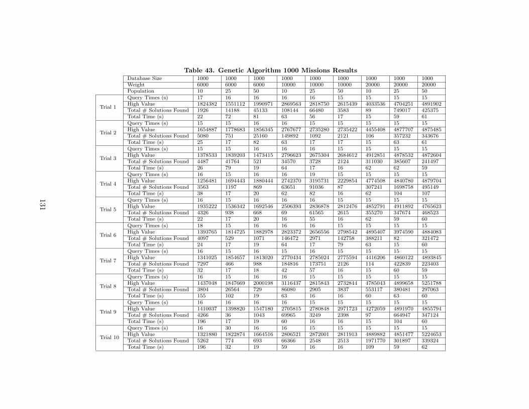
Table 43. Genetic Algorithm 1000 Missions ResultsDatabase Size 1000 1000 1000 1000 1000 1000 1000 1000 1000Weight 6000 6000 6000 10000 10000 10000 20000 20000 20000Population 10 25 50 10 25 50 10 25 50
Trial 1
Query Times (s) 17 16 16 16 16 15 15 15 15High Value 1824382 1551112 1990971 2869563 2818750 2615439 4033536 4704251 4891902Total # Solutions Found 1926 14188 45133 108144 66480 3583 89 749017 425375Total Time (s) 22 72 81 63 56 17 15 59 61
Trial 2
Query Times (s) 15 15 16 16 15 15 15 15 15High Value 1654887 1778683 1856345 2767677 2735280 2735422 4455408 4877707 4875485Total # Solutions Found 5080 751 25160 149892 1092 2121 106 357232 343676Total Time (s) 25 17 82 63 17 17 15 63 61
Trial 3
Query Times (s) 15 15 16 16 16 15 15 15 15High Value 1378533 1839203 1473415 2796623 2675304 2684612 4912851 4878532 4872604Total # Solutions Found 4487 41764 521 34570 3728 2124 311030 385607 241497Total Time (s) 26 79 19 64 17 16 62 62 59
Trial 4
Query Times (s) 16 15 16 16 19 15 15 15 15High Value 1256481 1694443 1880444 2742370 3195731 2229854 4774508 4840780 4879704Total # Solutions Found 3563 1197 869 63651 91036 87 307241 1698758 495149Total Time (s) 38 17 20 62 82 16 62 104 107
Trial 5
Query Times (s) 16 15 16 16 16 15 15 15 15High Value 1935222 1536342 1692546 2506393 2836878 2812476 4852791 4911892 4765623Total # Solutions Found 4326 938 668 69 61565 2615 355270 347674 468523Total Time (s) 22 17 20 16 55 16 62 59 60
Trial 6
Query Times (s) 18 15 16 16 16 15 15 15 15High Value 1393765 1814725 1882978 2823372 2656556 2798542 4895407 3974590 4884083Total # Solutions Found 4097 529 1071 146472 2971 142758 388211 82 321472Total Time (s) 24 17 19 64 17 79 63 15 60
Trial 7
Query Times (s) 16 15 16 15 16 15 15 15 15High Value 1341025 1854657 1813020 2770434 2785024 2775594 4416206 4860122 4893845Total # Solutions Found 7297 466 988 184816 173751 2126 114 422839 223403Total Time (s) 32 17 18 42 57 16 15 60 59
Trial 8
Query Times (s) 16 15 16 16 15 15 15 15 15High Value 1437048 1847669 2000198 3116437 2815843 2732844 4785043 4899658 5251788Total # Solutions Found 3804 26564 729 86080 2905 3837 553117 380481 297063Total Time (s) 155 102 19 63 16 16 60 63 60
Trial 9
Query Times (s) 16 16 16 16 15 15 15 15 15High Value 1410037 1398820 1547180 2705815 2780848 2971723 4272059 4891970 4855794Total # Solutions Found 4266 36 1043 69965 3249 2398 97 664947 347124Total Time (s) 196 17 19 60 16 16 15 104 60
Trial 10
Query Times (s) 16 30 16 16 15 15 15 15 15High Value 1321880 1822874 1664516 2806521 2872001 2811913 4889882 4851477 5224653Total # Solutions Found 5262 774 693 66366 2548 2513 1971770 301897 339324Total Time (s) 196 32 19 59 16 16 109 59 62
131

Table 44. HillClimber 100/1000 Missions Results
Database Size 100 100 100 1000 1000 1000Weight 6000 10000 20000 6000 10000 20000
Trial 1
Query Times (s) 1 1 1 18 16 16High Value 309817 1420066 4236426 521123 974609 2461836Total # Solutions Found 2 4 8 1 4 8Total Time (s) 2 1 1 18 17 16
Trial 2
Query Times (s) 1 1 1 16 16 16High Value 1381472 1265121 1238870 1190342 2069674 3460606Total # Solutions Found 4 2 1 3 4 6Total Time (s) 1 1 1 16 16 17
Trial 3
Query Times (s) 1 1 1 16 16 16High Value 1147166 1021666 3035028 1306170 2153661 4746294Total # Solutions Found 2 2 3 3 1 11Total Time (s) 1 1 1 16 17 16
Trial 4
Query Times (s) 1 1 1 16 16 16High Value 628935 2159280 3879872 1051911 2164604 4268168Total # Solutions Found 1 2 2 8 3 13Total Time (s) 1 1 1 16 16 16
Trial 5
Query Times (s) 1 1 1 16 16 16High Value 1005519 2198260 3238765 898947 2125600 3124768Total # Solutions Found 4 2 4 7 8 6Total Time (s) 1 1 1 17 16 16
Trial 6
Query Times (s) 1 1 1 16 16 16High Value 286475 1415617 3591181 815342 2716075 2004085Total # Solutions Found 2 2 7 7 4 3Total Time (s) 1 1 1 16 16 16
Trial 7
Query Times (s) 1 1 1 16 16 15High Value 1046692 1115558 2210963 873491 2441861 3528764Total # Solutions Found 1 2 2 3 3 8Total Time (s) 1 1 1 16 16 16
Trial 8
Query Times (s) 1 1 1 16 16 15High Value 1372693 1363302 3044141 957555 1976702 2721342Total # Solutions Found 2 1 3 4 7 6Total Time (s) 1 1 1 16 16 16
Trial 9
Query Times (s) 1 1 1 16 16 16High Value 828801 2175846 3044422 1181700 1627541 4165800Total # Solutions Found 3 4 5 5 3 6Total Time (s) 1 1 1 16 16 16
Trial 10
Query Times (s) 1 1 1 16 16 16High Value 759819 1887990 3360566 1254653 1971049 2707224Total # Solutions Found 2 2 5 1 7 6Total Time (s) 1 1 1 16 16 16
132
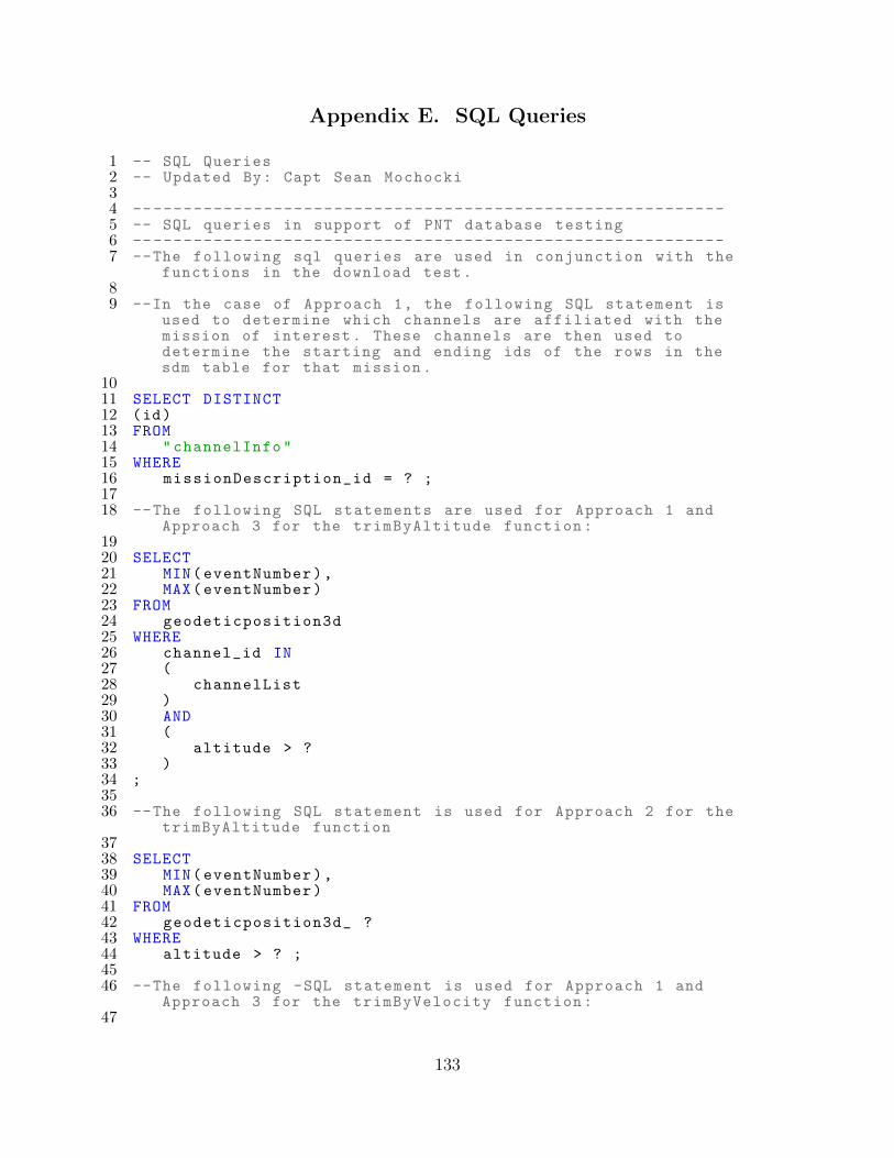
Appendix E. SQL Queries
1 -- SQL Queries2 -- Updated By: Capt Sean Mochocki34 -----------------------------------------------------------5 -- SQL queries in support of PNT database testing6 -----------------------------------------------------------7 --The following sql queries are used in conjunction with the
functions in the download test.89 --In the case of Approach 1, the following SQL statement is
used to determine which channels are affiliated with themission of interest. These channels are then used todetermine the starting and ending ids of the rows in thesdm table for that mission.
1011 SELECT DISTINCT12 (id)13 FROM14 "channelInfo"15 WHERE16 missionDescription_id = ? ;1718 --The following SQL statements are used for Approach 1 and
Approach 3 for the trimByAltitude function:1920 SELECT21 MIN(eventNumber),22 MAX(eventNumber)23 FROM24 geodeticposition3d25 WHERE26 channel_id IN27 (28 channelList29 )30 AND31 (32 altitude > ?33 )34 ;3536 --The following SQL statement is used for Approach 2 for the
trimByAltitude function3738 SELECT39 MIN(eventNumber),40 MAX(eventNumber)41 FROM42 geodeticposition3d_ ?43 WHERE44 altitude > ? ;4546 --The following -SQL statement is used for Approach 1 and
Approach 3 for the trimByVelocity function:47
133

48 SELECT49 MIN(g.eventNumber)50 FROM51 positionvelocityattitude g52 INNER JOIN53 "channelInfo" c54 ON c.id = g.channel_id55 WHERE56 channel_id IN57 (58 channelList59 )60 AND61 (62 velocity [1] > ?63 OR velocity [2] > ?64 OR velocity [3] > ?65 )66 ;6768 --The following SQL statement is used for Approach 2 for the
trimByVelocity function:6970 SELECT71 MIN(eventNumber)72 FROM73 positionvelocityattitude_ ?74 WHERE75 (76 velocity [1] > ?77 OR velocity [2] > ?78 OR velocity [3] > ?79 )80 ;8182 --The following SQL statements is used for Approach 1 to
determine what the minimum imu utime is for a user -specified mission.
8384 SELECT85 MIN(g.utime)86 FROM87 imu g88 INNER JOIN89 channelInfo c90 ON c.id = g.channel_id91 WHERE92 channel_id IN93 (94 channelList95 )96 ;9798 --The following SQL statement is used for Approach 1 to
determine the pivoting eventNumber for the trimByTimefunctions
99100 SELECT
134

101 MIN (g.eventNumber)102 FROM103 imu g104 INNER JOIN105 channelInfo c106 ON c.id = g.channel_id107 WHERE108 channel_id IN109 (110 channelList111 )112 AND g.utime >=113 (114 minEventNumber + time115 )116 ;117118 --The following SQL statements is used for Approach 2 to
determine what the minimum imu utime is for a userspecified mission.
119120 SELECT121 MIN(utime)122 FROM123 imu_ ?124125 --The following SQL statement is used for Approach 2 to
determine the pivoting eventNumber for the trimByTimefunctions
126127 SELECT128 MIN (g.eventNumber)129 FROM130 imu_ ?131 WHERE132 utime >=133 (134 minEventNumber + time135 )136 ;137138 --In the case of Approach 3, the same event numbers are
identified as for Approaches 1 and 2 by identifying theutime of the first imu event and then finding the eventnumber of the imu event which is at least a user specifiedlater utime.
139140 --The following sequence of SQL demonstrates the query series
utilized to determine the beginning and ending ids of anSDM table for a specific mission. For Approach 2 the firstand last ids of the table and mission of interest are justidentified directly , as they only correspond to thatspecific mission.
141142 SELECT DISTINCT143 (id)144 FROM145 "channelInfo"
135

146 WHERE147 missionDescription_id = ? ;148 SELECT149 min_max (eventNumber)150 FROM151 "tableName"152 WHERE153 channel_id IN154 (155 ?,156 ?,157 ...,158 ?159 )160 ;161 SELECT162 min_max(id)163 FROM164 "tableName"165 WHERE166 channel_id IN167 (168 ?,169 ?,170 ...,171 ?172 )173 AND174 (175 eventNumber = ?176 )177 ;178179 --The following statement is the SQL statement which generates
the result set with the necessary information to recreatethe original imu LCM Event
180 SELECT181 c.channelname ,182 g.utime ,183 g.eventNumber ,184 c.deviceid ,185 g.timestamp_arrival_sec ,186 g.timestamp_arrival_nsec ,187 g.timestamp_valid_sec ,188 g.timestamp_valid_nsec ,189 g.seqnumber ,190 g.delta_v ,191 g.delta_theta ,192 FROM193 "channelInfo" c194 INNER JOIN195 imu g196 ON g.channel_id = c.id197 WHERE198 g.id BETWEEN (next_sdm_id) AND199 (200 next_sdm_id + bundle_size - 1201 )
136
202 ;203204 --metaData Tests205 --The following SQL statements are used with conjunction with
the vehicleTestViewUpdate function.206207 DROP VIEW IF EXISTS vehicleClass;208 CREATE VIEW vehicleClass AS209 SELECT DISTINCT210 m.id,211 v.vehicle212 FROM213 "channelInfo" c214 INNER JOIN215 "missionDescription" m216 ON m.id = c.missionDescription_id217 INNER JOIN218 sensorInstallationInfo s219 ON c.sensorInstallation_id = s.id220 INNER JOIN221 vehicle v222 ON v.id = s.sensorModel_id223 ORDER BY224 m.id;225 SELECT226 id227 FROM228 vehicleClass229 WHERE230 vehicle = ’randomVehicle ’;231232 --The following SQL statements are used in conjunction with
the sensorTypeTestWithView function.233234 DROP VIEW IF EXISTS sensorTypes;235 CREATE VIEW sensorTypes AS236 SELECT DISTINCT237 m.id,238 sm.type239 FROM240 "channelInfo" c241 INNER JOIN242 "missionDescription" m243 ON m.id = c.missionDescription_id244 INNER JOIN245 sensorInstallationInfo s246 ON c.sensorInstallation_id = s.id247 INNER JOIN248 sensorModel sm249 ON sm.id = s.sensorModel_id250 ORDER BY251 m.id;252 SELECT253 id254 FROM255 sensorTypes256 WHERE257 type = ’randomSensorTypes ’;
137

258259 SELECT DISTINCT260 a.id261 from262 sensorTypes a263 INNER JOIN264 sensorTypes b265 ON a.id = b.id266 WHERE267 a.type = ’randomType1 ’268 AND b.type = ’randomType2 ’;269270 --The following SQL statements are used in conjuction with the
weatherTest function.271272 WITH Temporary AS273 (274 SELECT DISTINCT275 missionDescription_id ,276 skycover277 FROM278 "skyCover"279 ORDER BY280 missionDescription_id281 )282 SELECT283 missionDescription_id284 FROM285 Temporary286 WHERE287 skycover = ’randomSkyCover ’;288289 WITH Temporary AS290 (291 SELECT DISTINCT292 missionDescription_id ,293 obscuration294 FROM295 "obscuration"296 ORDER BY297 missionDescription_id298 )299 SELECT300 missionDescription_id301 FROM302 Temporary303 WHERE304 obscuration = ’randomObscuration ’;305306 WITH Temporary AS307 (308 SELECT DISTINCT309 missionDescription_id ,310 precipitation311 FROM312 "precipitation"313 ORDER BY314 missionDescription_id
138
315 )316 SELECT317 missionDescription_id318 FROM319 Temporary320 WHERE321 precipitation = ’randomPrecipitation ’;322323324 --The following SELECT query uses the sensorTypes view to
perform the sensorQualityTestWithView. thesensorQualityTestWithoutSensorTypesView is similar , exceptthat the content of the sensorTypes view is createdtemporarily as part of the query.
325326 WITH Temporary AS327 (328 SELECT DISTINCT329 m.id,330 ss.sensorUID ,331 imu.timeCorrelated_accelBiasSigma ,332 imu.timeCorrelated_accelBiasTau ,333 imu.timeCorrelated_gyroBiasSigma ,334 imu.timeCorrelated_gyroBiasTau ,335 imu.velocityRandomWalk ,336 imu.angularRandomWalk ,337 imu.accelerometerScaleFactorUncertainty ,338 imu.gyroScaleFactorUncertainty339 FROM340 "channelInfo" c341 INNER JOIN342 "missionDescription" m343 ON m.id = c.missionDescription_id344 INNER JOIN345 "sensorInstallationInfo" s346 ON c.sensorInstallation_id = s.id347 INNER JOIN348 "sensorSpecific" ss349 ON s.sensorSpecific_id = ss.id350 INNER JOIN351 "IMU_Intrinsic" imu352 ON imu.sensorSpecific_id = ss.id353 INNER JOIN354 sensorTypes a355 ON a.type = ’IMU’356 ORDER BY357 m.id358 )359360 SELECT DISTINCT id FROM Temporary WHERE (361 timeCorrelated_accelBiasSigma > random362 AND timeCorrelated_accelBiasTau > random363 AND timeCorrelated_gyraBiasSigma > random364 AND timeCorrelated_gyroBiasTau > random365 AND velocityRandomWalk > random366 AND angularRandomWalk > random367 )368 ORDER BY
139

369 id;370371 --The following query provides the necessary information for
the maneuver test.372373 WITH Temporary AS374 (375 SELECT376 missionDescription_id , maneuver , approximate_duration377 FROM378 maneuvers379 ORDER BY380 id)381 SELECT382 missionDescription_id383 FROM384 Temporary385 WHERE386 maneuver = randomManeuver387 ORDER BY388 id;389390 The following query provides the necessary information for the
terrainSingleQueryTest391392 SELECT DISTINCT393 m.id,394 t.terrain395 FROM396 terrain.t397 INNER JOIN398 "missionDescription" m399 ON m.id = t.missionDescription_id400 ORDER BY401 m.id;402403 Data Tests404405 --The following query is used for the testVelocity function
and is run against the min and max ids for every mission inApproach 1 and Approach 3. The query for Approach 2 is thesame except that the tableName specifies the mission of
interest and the requirement for minimum and maximum ids isnot included.
406407 SELECT408 EXISTS409 (410 SELECT411 1412 FROM413 positionvelocityattitude414 WHERE415 (416 velocity [1] > ?417 OR velocity [2] > ?418 OR velocity [3] > ?419 )
140

420 AND421 (422 id BETWEEN id_min AND id_max423 )424 )425 ;426427 --The following query is used for the testLatLongBoundingBox
function and is run against the min and max ids for everymission in Approach 1 and Approach 3. Like withtestVelocity , the Approach 2 query is the same with theexception of the tableName and not requiring the min andmax ids.
428 SELECT429 EXISTS430 (431 SELECT432 1433 FROM434 geodeticposition3d435 WHERE436 (437 ( latitude > latLow438 AND latitude < latHigh)439 AND440 (441 longitude > longLow442 AND longitude < longHigh443 )444 AND445 (446 id BETWEEN id_min AND id_max447 )448 )449 )450 ;451452453 --The following query is used for testPlatformDynamics
Approaches 1 and 2, with the difference of not needing toidentify the beginning and ending ids on Approach 2. ForApproach 3, the original file is downloaded and then parsedline by line identifying imu events , with the program
recording what the delta velocity is for the prior event sothat the acceleration can be calculated.
454455 WITH acceleration AS456 (457 SELECT458 ((imu2.delta_v [1] - imu1.delta_v [1]) / (imu2.utime - imu1.
utime))*1000000 AS accel_x ,459 (460 (imu2.delta_v [2] - imu1.delta_v [2]) / (imu2.utime - imu1.utime
)461 )462 *1000000 AS accel_y ,463 (
141

464 (imu2.delta_v [3] - imu1.delta_v [3]) / (imu2.utime - imu1.utime)
465 )466 *1000000 AS accel_z467 FROM468 imu imu1469 INNER JOIN470 imu imu2471 ON (imu2.id = imu1.id + 1)472 WHERE473 (474 imu1.channel_id IN channel_id475 )476 AND477 (478 imu2.channel_id IN channel_id479 )480 ORDER BY481 imu1.id482 )483 SELECT484 EXISTS485 (486 SELECT487 1488 FROM489 acceleration490 WHERE491 ABS(sqrt(POWER(accel_x , 2) + POWER(accel_y , 2) +
POWER(accel_z , 2)) - 9.81) BETWEEN (2*9.81) AND492 (493 4*9.81494 )495 )496 ;497498 --The testTimeOfDay follows the previously discussed process
for identifying the first and last ids for the mission ofinterest in the imu table , and then identifies the utimefor those two rows. For Approach 3, the file is downloadedand the utime for the first and last imu events is read.The SQL for this query is below:
499500 SELECT501 utime502 FROM503 imu504 WHERE505 id = imu_min506 AND eventNumber = eventNumber_min;507 SELECT508 utime509 FROM510 imu511 WHERE512 id = imu_max513 AND eventNumber = eventNumber_max;514
142
515 --For testSatelliteSystem , the following query is used forApproaches 1 and 2:
516517 SELECT518 EXISTS519 (520 SELECT521 1522 FROM523 gnss524 WHERE525 ’SYS_G’ = ANY(satellite_system)526 AND id BETWEEN min_id AND max_id527 )528 ;
143

Appendix F. SQL Database and Index Scripts
1 -- SQL Database Creation Scripts2 -- Updated By: Capt Sean Mochocki34 -- Database script used in the creation of Approach1 Database5 CREATE TABLE IF NOT EXISTS "missionDescription" (id SERIAL
PRIMARY KEY , startDate_UTC DATE , endDate_UTC DATE ,organization TEXT , missionLocationSTART TEXT ,missionLocationEnd TEXT , missionLength_Seconds BIGINT ,dataFileSize BIGINT , fileName Text);
6 DO $$7 BEGIN8 CREATE TYPE vehicle_type AS ENUM (’PLANE’, ’GROUND_VEHICLE ’
, ’PEDESTRIAN ’, ’MISSILE ’, ’UAV’, ’SUB’);9 EXCEPTION
10 WHEN11 duplicate_object12 THEN13 null;14 END15 $$ ;16 CREATE TABLE IF NOT EXISTS "aircraft" (id SERIAL PRIMARY KEY ,
aircraftType TEXT , tailNumber TEXT);17 CREATE TABLE IF NOT EXISTS "groundVehicle" (id SERIAL PRIMARY
KEY , make TEXT , model TEXT , year INTEGER);18 CREATE TABLE IF NOT EXISTS vehicle (id SERIAL PRIMARY KEY ,
vehicle vehicle_type , groundVehicle_id INTEGER REFERENCES "groundVehicle" (id), aircraft_id INTEGER REFERENCES "aircraft"(id));
19 DO $$20 BEGIN21 CREATE TYPE sensor_type AS ENUM (’BAROMETER ’, ’MAGNETOMETER
’, ’GPS’, ’IMS’, ’CLOCK’, ’CAMERA ’, ’IMU’, ’GNSS’);22 EXCEPTION23 WHEN24 duplicate_object25 THEN26 null;27 END28 $$ ;29 CREATE TABLE IF NOT EXISTS "sensorModel" (id SERIAL PRIMARY
KEY , model TEXT , manufacturer TEXT , type sensor_type ,UNIQUE (model , manufacturer , type));
30 CREATE TABLE IF NOT EXISTS "extrinsicSensorConfiguration" (idSERIAL PRIMARY KEY , leverArm DOUBLE PRECISION [3],orientationX DOUBLE PRECISION [3], orientationY DOUBLEPRECISION [3], orientationZ DOUBLE PRECISION [3]);
31 CREATE TABLE IF NOT EXISTS "sensorSpecific" (id SERIAL PRIMARYKEY , sensorUID TEXT);
32 CREATE TABLE IF NOT EXISTS "GPS_Intrinsic" (id SERIAL PRIMARYKEY , gps_antenna_make TEXT , gps_antenna_model TEXT ,sensorSpecific_id INTEGER REFERENCES "sensorSpecific" (id));
33 CREATE TABLE IF NOT EXISTS "externalAidingClock" (id SERIALPRIMARY KEY , make TEXT , model TEXT , GPS_Intrinsic_idINTEGER REFERENCES "GPS_Intrinsic" (id));
144

34 CREATE TABLE IF NOT EXISTS "system_signals_Tracked" (id SERIALPRIMARY KEY , systemTracked TEXT , signalTracked TEXT ,
GPS_Intrinsic_id INTEGER REFERENCES "GPS_Intrinsic" (id));35 CREATE TABLE IF NOT EXISTS "supportedAugmentationSystems" (id
SERIAL PRIMARY KEY , supportedAugmentationSystem TEXT ,GPS_Intrinsic_id INTEGER REFERENCES "GPS_Intrinsic" (id));
36 CREATE TABLE IF NOT EXISTS "IMU_Intrinsic" (id SERIAL PRIMARYKEY , timeCorrelated_accelBiasSigma DOUBLE PRECISION [3],timeCorrelated_accelBiasTau DOUBLE PRECISION [3],timeCorrelated_gyroBiasSigma DOUBLE PRECISION [3],timeCorrelated_gyroBiasTau DOUBLE PRECISION [3],velocityRandomWalk DOUBLE PRECISION [3], angularRandomWalkDOUBLE PRECISION [3], accelerometerScaleFactorUncertaintyDOUBLE PRECISION , gyroScaleFactorUncertainty DOUBLEPRECISION , sensorSpecific_id INTEGER REFERENCES "sensorSpecific" (id));
37 CREATE TABLE IF NOT EXISTS "clock_Intrinsic" (id SERIALPRIMARY KEY , h0 DOUBLE PRECISION , h1 DOUBLE PRECISION , h2DOUBLE PRECISION , x0Array DOUBLE PRECISION [], p0ArrayDOUBLE PRECISION [], sensorSpecific_id INTEGER REFERENCES "sensorSpecific" (id));
38 CREATE TABLE IF NOT EXISTS "camera" (id SERIAL PRIMARY KEY ,focalLength DOUBLE PRECISION , cameraImageCenter DOUBLEPRECISION [3][3] , lensDistortion DOUBLE PRECISION [5],sensorSpecific_id INTEGER REFERENCES "sensorSpecific" (id));
39 CREATE TABLE IF NOT EXISTS "sensorInstallationInfo" (id SERIALPRIMARY KEY , sensorModel_id INTEGER REFERENCES "
sensorModel" (id), sensorSpecific_id INTEGER REFERENCES "sensorSpecific" (id), extrinsicSensorConfiguration_idINTEGER REFERENCES "extrinsicSensorConfiguration" (id),vehicle_id INTEGER REFERENCES "vehicle" (id));
40 CREATE TABLE IF NOT EXISTS "channelInfo" (id SERIAL PRIMARYKEY , channelName TEXT , channelUse TEXT , deviceID TEXT ,truth BOOLEAN , missionDescription_id INTEGER REFERENCES "missionDescription" (id), sensorInstallation_id INTEGERREFERENCES "sensorInstallationInfo" (id), UNIQUE (id,missionDescription_id));
41 CREATE TABLE IF NOT EXISTS "outage" (id SERIAL PRIMARY KEY ,planned BOOLEAN , approximate_duration INT , intermittentBOOLEAN , missionDescription_id INTEGER REFERENCES "missionDescription" (id), UNIQUE (id, missionDescription_id));
42 CREATE TABLE IF NOT EXISTS "outage_channel" (channel_idINTEGER REFERENCES "channelInfo" (id), outage_id INTEGERREFERENCES outage (id), missionDescription_id INTEGERREFERENCES "missionDescription" (id), FOREIGN KEY (outage_id , missionDescription_id) REFERENCES outage (id ,missionDescription_id));
43 CREATE TABLE IF NOT EXISTS "velocity3d" (id SERIAL PRIMARY KEY, timeStamp_arrival_sec BIGINT , timeStamp_arrival_nsec INT ,timeStamp_valid_sec BIGINT , timeStamp_valid_nsec INT ,
utime BIGINT , eventNumber BIGINT , seqNumber BIGINT ,logByteOffset BIGINT , x DOUBLE PRECISION , y DOUBLEPRECISION , z DOUBLE PRECISION , covariance DOUBLE PRECISION[3][3] , channel_id INTEGER REFERENCES "channelInfo" (id));
44 CREATE TABLE IF NOT EXISTS "velocity1d" (id SERIAL PRIMARY KEY, timeStamp_arrival_sec BIGINT , timeStamp_arrival_nsec INT ,
145

timeStamp_valid_sec BIGINT , timeStamp_valid_nsec INT ,utime BIGINT , eventNumber BIGINT , seqNumber BIGINT ,logByteOffset BIGINT , x DOUBLE PRECISION , variance DOUBLEPRECISION , channel_id INTEGER REFERENCES "channelInfo" (id));
45 CREATE TABLE IF NOT EXISTS "speed" (id SERIAL PRIMARY KEY ,timeStamp_arrival_sec BIGINT , timeStamp_arrival_nsec INT ,timeStamp_valid_sec BIGINT , timeStamp_valid_nsec INT , utimeBIGINT , eventNumber BIGINT , seqNumber BIGINT ,
logByteOffset BIGINT , speed DOUBLE PRECISION , varianceDOUBLE PRECISION , channel_id INTEGER REFERENCES "channelInfo" (id));
46 CREATE TABLE IF NOT EXISTS "altitude" (id SERIAL PRIMARY KEY ,timeStamp_arrival_sec BIGINT , timeStamp_arrival_nsec INT ,timeStamp_valid_sec BIGINT , timeStamp_valid_nsec INT , utimeBIGINT , eventNumber BIGINT , seqNumber BIGINT ,
logByteOffset BIGINT , altitude DOUBLE PRECISION , varianceDOUBLE PRECISION , channel_id INTEGER REFERENCES "channelInfo" (id));
47 CREATE TABLE IF NOT EXISTS "geodeticposition3d" (id SERIALPRIMARY KEY , timeStamp_arrival_sec BIGINT ,timeStamp_arrival_nsec INT , timeStamp_valid_sec BIGINT ,timeStamp_valid_nsec INT , utime BIGINT , eventNumber BIGINT ,seqNumber BIGINT , logByteOffset BIGINT , latitude DOUBLE
PRECISION , longitude DOUBLE PRECISION , altitude DOUBLEPRECISION , covariance DOUBLE PRECISION [3][3] , channel_idINTEGER REFERENCES "channelInfo" (id));
48 CREATE TABLE IF NOT EXISTS "threeaxismagnetometer" (id SERIALPRIMARY KEY , timeStamp_arrival_sec BIGINT ,timeStamp_arrival_nsec INT , timeStamp_valid_sec BIGINT ,timeStamp_valid_nsec INT , utime BIGINT , eventNumber BIGINT ,seqNumber BIGINT , logByteOffset BIGINT , field DOUBLE
PRECISION [3], covariance DOUBLE PRECISION [3][3] ,channel_id INTEGER REFERENCES "channelInfo" (id));
49 CREATE TABLE IF NOT EXISTS "positionvelocityattitude" (idSERIAL PRIMARY KEY , timeStamp_arrival_sec BIGINT ,timeStamp_arrival_nsec INT , timeStamp_valid_sec BIGINT ,timeStamp_valid_nsec INT , utime BIGINT , eventNumber BIGINT ,seqNumber BIGINT , logByteOffset BIGINT , latitude DOUBLE
PRECISION , longitude DOUBLE PRECISION , altitude DOUBLEPRECISION , velocity DOUBLE PRECISION [3], attitude DOUBLEPRECISION [3], covariance DOUBLE PRECISION [9][9] ,channel_id INTEGER REFERENCES "channelInfo" (id));
50 DO $$51 BEGIN52 CREATE TYPE encoding AS ENUM (’RAW_GRAY8 ’, ’RAW_RGB8 ’, ’
RAW_BGR8 ’, ’RAW_RGBA8 ’, ’JPG’, ’PNG’);53 EXCEPTION54 WHEN55 duplicate_object56 THEN57 null;58 END59 $$ ;60 CREATE TABLE IF NOT EXISTS "opticalcameraimage" (id SERIAL
PRIMARY KEY , timeStamp_arrival_sec BIGINT ,timeStamp_arrival_nsec INT , timeStamp_valid_sec BIGINT ,timeStamp_valid_nsec INT , utime BIGINT , eventNumber BIGINT ,
146
seqNumber BIGINT , logByteOffset BIGINT , encoding encoding ,height INT , width INT , num_channels INT , array_length INT ,data BYTEA , channel_id INTEGER REFERENCES "channelInfo" (
id));61 CREATE TABLE IF NOT EXISTS "imu" (id SERIAL PRIMARY KEY ,
timeStamp_arrival_sec BIGINT , timeStamp_arrival_nsec INT ,timeStamp_valid_sec BIGINT , timeStamp_valid_nsec INT , utimeBIGINT , eventNumber BIGINT , seqNumber BIGINT ,
logByteOffset BIGINT , delta_v DOUBLE PRECISION [3],delta_theta DOUBLE PRECISION [3], channel_id INTEGERREFERENCES "channelInfo" (id));
62 DO $$63 BEGIN64 CREATE TYPE satellite_system AS ENUM (’SYS_G’, ’SYS_R’, ’
SYS_E ’, ’SYS_J ’, ’SYS_C ’, ’SYS_I ’, ’SYS_S ’, ’SYS_M ’, ’SYS_O ’);
65 EXCEPTION66 WHEN67 duplicate_object68 THEN69 null;70 END71 $$ ;72 DO $$73 BEGIN74 CREATE TYPE type AS ENUM (’OBS_C’, ’OBS_L’, ’OBS_D’, ’OBS_S
’, ’OBS_I’);75 EXCEPTION76 WHEN77 duplicate_object78 THEN79 null;80 END81 $$ ;82 DO $$83 BEGIN84 CREATE TYPE band AS ENUM (’BAND1’, ’BAND2’, ’BAND5’, ’BAND6
’, ’BAND7’, ’BAND8’, ’BAND9’, ’BAND0’);85 EXCEPTION86 WHEN87 duplicate_object88 THEN89 null;90 END91 $$ ;92 DO $$93 BEGIN94 CREATE TYPE attribute AS ENUM (’SIG_P’, ’SIG_C’, ’SIG_D’, ’
SIG_Y’, ’SIG_M ’, ’SIG_N ’, ’SIG_A ’, ’SIG_B ’, ’SIG_I ’, ’SIG_Q’, ’SIG_S ’, ’SIG_L ’, ’SIG_X ’, ’SIG_W ’, ’SIG_Z ’, ’SIG_BLANK ’);
95 EXCEPTION96 WHEN97 duplicate_object98 THEN99 null;
100 END101 $$ ;
147

102 DO $$103 BEGIN104 CREATE TYPE time_system AS ENUM (’TIME_GLO ’, ’TIME_GPS ’, ’
TIME_GAL ’, ’TIME_BDT ’);105 EXCEPTION106 WHEN107 duplicate_object108 THEN109 null;110 END111 $$ ;112 CREATE TABLE IF NOT EXISTS "gnss" (id SERIAL PRIMARY KEY ,
timeStamp_arrival_sec BIGINT , timeStamp_arrival_nsec INT ,timeStamp_valid_sec BIGINT , timeStamp_valid_nsec INT , utimeBIGINT , eventNumber BIGINT , seqNumber BIGINT ,
logByteOffset BIGINT , --week_number INTEGER ,seconds_of_week DOUBLE PRECISION , time_system TEXT ,
113 week_number INTEGER , seconds_of_week DOUBLE PRECISION ,time_system time_system , epoch_flag INTEGER , num_satellitesINTEGER , num_measurements INTEGER , obs_prn INT [],
satellite_system satellite_system [], type type [], bandband [], attribute attribute [], observation DOUBLEPRECISION [], LLI INT [], signal_strength INT [],lock_count INT [], channel_id INTEGER REFERENCES "channelInfo" (id));
114 CREATE TABLE IF NOT EXISTS "gpsephemeris" (id SERIAL PRIMARYKEY , timeStamp_arrival_sec BIGINT , timeStamp_arrival_nsecINT , timeStamp_valid_sec BIGINT , timeStamp_valid_nsec INT ,utime BIGINT , eventNumber BIGINT , seqNumber BIGINT ,logByteOffset BIGINT , prn INTEGER , wn_t_oc INTEGER , t_ocDOUBLE PRECISION , t_gd DOUBLE PRECISION , af_0 DOUBLEPRECISION , af_1 DOUBLE PRECISION , af_2 DOUBLE PRECISION ,m_0 DOUBLE PRECISION , delta_n DOUBLE PRECISION , e DOUBLEPRECISION , sqrt_a DOUBLE PRECISION , omega_0 DOUBLEPRECISION , i_0 DOUBLE PRECISION , i_dot DOUBLE PRECISION ,omega DOUBLE PRECISION , omega_dot DOUBLE PRECISION , c_ucDOUBLE PRECISION , c_us DOUBLE PRECISION , c_rc DOUBLEPRECISION , c_rs DOUBLE PRECISION , c_ic DOUBLE PRECISION ,c_is DOUBLE PRECISION , wn_t_oe INTEGER , t_oe DOUBLEPRECISION , channel_id INTEGER REFERENCES "channelInfo" (id));
115 CREATE TABLE IF NOT EXISTS "sensorRegistrationAck" (id SERIALPRIMARY KEY , utime BIGINT , eventNumber BIGINT ,logByteOffset BIGINT , registered boolean , sensorUID TEXT ,channel_id INTEGER REFERENCES "channelInfo" (id));
116 CREATE TABLE IF NOT EXISTS "non_SDM_Message" (id SERIALPRIMARY KEY , utime BIGINT , eventNumber BIGINT ,logByteOffset BIGINT , data bytea , channel_id INTEGERREFERENCES "channelInfo" (id));
117 DO $$118 BEGIN119 CREATE TYPE precipitation_type AS ENUM (’RAIN’, ’SNOW’, ’
SLEET ’, ’HAIL’);120 EXCEPTION121 WHEN122 duplicate_object123 THEN124 null;
148
125 END126 $$ ;127 DO $$128 BEGIN129 CREATE TYPE intensity AS ENUM (’LIGHT’, ’MODERATE ’, ’HIGH’)
;130 EXCEPTION131 WHEN132 duplicate_object133 THEN134 null;135 END136 $$ ;137 CREATE TABLE IF NOT EXISTS "precipitation" (precipitation
precipitation_type , intensity intensity ,missionDescription_id INTEGER REFERENCES "missionDescription" (id), PRIMARY KEY (precipitation ,intensity , missionDescription_id));
138 DO $$139 BEGIN140 CREATE TYPE obscuration_type AS ENUM (’FOG’, ’MIST’, ’SMOKE
’, ’DUST’);141 EXCEPTION142 WHEN143 duplicate_object144 THEN145 null;146 END147 $$ ;148 CREATE TABLE IF NOT EXISTS "obscuration" (obscuration
obscuration_type , missionDescription_id INTEGER REFERENCES"missionDescription" (id), PRIMARY KEY (obscuration ,missionDescription_id));
149 DO $$150 BEGIN151 CREATE TYPE terrain_type AS ENUM (’DESERT ’, ’FOREST ’, ’
URBAN ’, ’MOUNTAINS ’, ’WATER ’);152 EXCEPTION153 WHEN154 duplicate_object155 THEN156 null;157 END158 $$ ;159 CREATE TABLE iF NOT EXISTS "terrain" (terrain terrain_type ,
missionDescription_id INTEGER REFERENCES "missionDescription"(id), PRIMARY KEY (terrain ,missionDescription_id));
160 DO $$161 BEGIN162 CREATE TYPE skyCover AS ENUM (’CLOUDY ’, ’MOSTLY_CLOUDY ’, ’
PARTLY_SUNNY ’, ’MOSTLY_SUNNY ’, ’SUNNY’);163 EXCEPTION164 WHEN165 duplicate_object166 THEN167 null;168 END
149
169 $$ ;170 CREATE TABLE IF NOT EXISTS "skyCover" (skyCover skycover ,
missionDescription_id INTEGER REFERENCES "missionDescription"(id), PRIMARY KEY (skyCover ,missionDescription_id));
171 DO $$172 BEGIN173 CREATE TYPE maneuver AS ENUM (’FIGURE_EIGHT ’, ’FIGURE_S ’, ’
CIRCLE ’, ’ELLIPSE ’, ’SPIRAL ’, ’INVERSION ’);174 EXCEPTION175 WHEN176 duplicate_object177 THEN178 null;179 END180 $$ ;181 CREATE TABLE IF NOT EXISTS "maneuvers" (id SERIAL PRIMARY KEY ,
maneuver maneuver , approximate_duration INTEGER ,missionDescription_id INTEGER REFERENCES "missionDescription"(id));
182 CREATE TABLE IF NOT EXISTS "loopClosures" (id SERIAL PRIMARYKEY , time TIME , latitude DOUBLE PRECISION , longitude DOUBLEPRECISION , missionDescription_id INTEGER REFERENCES "
missionDescription" (id));183 CREATE TABLE IF NOT EXISTS "wayPoints" (id SERIAL PRIMARY KEY ,
time TIME , latitude DOUBLE PRECISION , longitude DOUBLEPRECISION , missionDescription_id INTEGER REFERENCES "missionDescription" (id));
184 CREATE TABLE IF NOT EXISTS "altitudeSegments" (id SERIALPRIMARY KEY , start_altitude INTEGER , end_altitude INTEGER ,approximate_duration INTEGER , missionDescription_id INTEGERREFERENCES "missionDescription" (id));
185 CREATE TABLE IF NOT EXISTS "unexpectedResults" (id SERIALPRIMARY KEY , unexpectedResults TEXT);
186187 -- Database script used in the creation of Approach2 Database188 CREATE TABLE IF NOT EXISTS "missionDescription" (id SERIAL
PRIMARY KEY , startDate_UTC DATE , endDate_UTC DATE ,organization TEXT , missionLocationSTART TEXT ,missionLocationEnd TEXT , missionLength_Seconds BIGINT ,dataFileSize BIGINT , fileName Text);
189 DO $$190 BEGIN191 CREATE TYPE vehicle_type AS ENUM (’PLANE’, ’GROUND_VEHICLE ’
, ’PEDESTRIAN ’, ’MISSILE ’, ’UAV’, ’SUB’);192 EXCEPTION193 WHEN194 duplicate_object195 THEN196 null;197 END198 $$ ;199 CREATE TABLE IF NOT EXISTS "aircraft" (id SERIAL PRIMARY KEY ,
aircraftType TEXT , tailNumber TEXT);200 CREATE TABLE IF NOT EXISTS "groundVehicle" (id SERIAL PRIMARY
KEY , make TEXT , model TEXT , year INTEGER);201 CREATE TABLE IF NOT EXISTS vehicle (id SERIAL PRIMARY KEY ,
vehicle vehicle_type , groundVehicle_id INTEGER REFERENCES "
150
groundVehicle" (id), aircraft_id INTEGER REFERENCES "aircraft"(id));
202 DO $$203 BEGIN204 CREATE TYPE sensor_type AS ENUM (’BAROMETER ’, ’MAGNETOMETER
’, ’GPS’, ’IMS’, ’CLOCK’, ’CAMERA ’, ’IMU’, ’GNSS’);205 EXCEPTION206 WHEN207 duplicate_object208 THEN209 null;210 END211 $$ ;212 CREATE TABLE IF NOT EXISTS "sensorModel" (id SERIAL PRIMARY
KEY , model TEXT , manufacturer TEXT , type sensor_type ,UNIQUE (model , manufacturer , type));
213 CREATE TABLE IF NOT EXISTS "extrinsicSensorConfiguration" (idSERIAL PRIMARY KEY , leverArm DOUBLE PRECISION [3],orientationX DOUBLE PRECISION [3], orientationY DOUBLEPRECISION [3], orientationZ DOUBLE PRECISION [3]);
214 CREATE TABLE IF NOT EXISTS "sensorSpecific" (id SERIAL PRIMARYKEY , sensorUID TEXT);
215 CREATE TABLE IF NOT EXISTS "GPS_Intrinsic" (id SERIAL PRIMARYKEY , gps_antenna_make TEXT , gps_antenna_model TEXT ,sensorSpecific_id INTEGER REFERENCES "sensorSpecific" (id));
216 CREATE TABLE IF NOT EXISTS "externalAidingClock" (id SERIALPRIMARY KEY , make TEXT , model TEXT , GPS_Intrinsic_idINTEGER REFERENCES "GPS_Intrinsic" (id));
217 CREATE TABLE IF NOT EXISTS "system_signals_Tracked" (id SERIALPRIMARY KEY , systemTracked TEXT , signalTracked TEXT ,
GPS_Intrinsic_id INTEGER REFERENCES "GPS_Intrinsic" (id));218 CREATE TABLE IF NOT EXISTS "supportedAugmentationSystems" (id
SERIAL PRIMARY KEY , supportedAugmentationSystem TEXT ,GPS_Intrinsic_id INTEGER REFERENCES "GPS_Intrinsic" (id));
219 CREATE TABLE IF NOT EXISTS "IMU_Intrinsic" (id SERIAL PRIMARYKEY , timeCorrelated_accelBiasSigma DOUBLE PRECISION [3],timeCorrelated_accelBiasTau DOUBLE PRECISION [3],timeCorrelated_gyroBiasSigma DOUBLE PRECISION [3],timeCorrelated_gyroBiasTau DOUBLE PRECISION [3],velocityRandomWalk DOUBLE PRECISION [3], angularRandomWalkDOUBLE PRECISION [3], accelerometerScaleFactorUncertaintyDOUBLE PRECISION , gyroScaleFactorUncertainty DOUBLEPRECISION , sensorSpecific_id INTEGER REFERENCES "sensorSpecific" (id));
220 CREATE TABLE IF NOT EXISTS "clock_Intrinsic" (id SERIALPRIMARY KEY , h0 DOUBLE PRECISION , h1 DOUBLE PRECISION , h2DOUBLE PRECISION , x0Array DOUBLE PRECISION [], p0ArrayDOUBLE PRECISION [], sensorSpecific_id INTEGER REFERENCES "sensorSpecific" (id));
221 CREATE TABLE IF NOT EXISTS "camera" (id SERIAL PRIMARY KEY ,focalLength DOUBLE PRECISION , cameraImageCenter DOUBLEPRECISION [3][3] , lensDistortion DOUBLE PRECISION [5],sensorSpecific_id INTEGER REFERENCES "sensorSpecific" (id));
222 CREATE TABLE IF NOT EXISTS "sensorInstallationInfo" (id SERIALPRIMARY KEY , sensorModel_id INTEGER REFERENCES "
sensorModel" (id), sensorSpecific_id INTEGER REFERENCES "
151

sensorSpecific" (id), extrinsicSensorConfiguration_idINTEGER REFERENCES "extrinsicSensorConfiguration" (id),vehicle_id INTEGER REFERENCES "vehicle" (id));
223 CREATE TABLE IF NOT EXISTS "channelInfo" (id SERIAL PRIMARYKEY , channelName TEXT , channelUse TEXT , deviceID TEXT ,truth BOOLEAN , missionDescription_id INTEGER REFERENCES "missionDescription" (id), sensorInstallation_id INTEGERREFERENCES "sensorInstallationInfo" (id), UNIQUE (id,missionDescription_id));
224 CREATE TABLE IF NOT EXISTS "outage" (id SERIAL PRIMARY KEY ,planned BOOLEAN , approximate_duration INT , intermittentBOOLEAN , missionDescription_id INTEGER REFERENCES "missionDescription" (id), UNIQUE (id, missionDescription_id));
225 CREATE TABLE IF NOT EXISTS "outage_channel" (channel_idINTEGER REFERENCES "channelInfo" (id), outage_id INTEGERREFERENCES outage (id), missionDescription_id INTEGERREFERENCES "missionDescription" (id), FOREIGN KEY (outage_id , missionDescription_id) REFERENCES outage (id ,missionDescription_id));
226 CREATE TABLE IF NOT EXISTS "velocity3d_*" (id SERIAL PRIMARYKEY , timeStamp_arrival_sec BIGINT , timeStamp_arrival_nsecINT , timeStamp_valid_sec BIGINT , timeStamp_valid_nsec INT ,utime BIGINT , eventNumber BIGINT , seqNumber BIGINT ,logByteOffset BIGINT , x DOUBLE PRECISION , y DOUBLEPRECISION , z DOUBLE PRECISION , covariance DOUBLE PRECISION[3][3] , channel_id INTEGER REFERENCES "channelInfo" (id));
227 CREATE TABLE IF NOT EXISTS "velocity1d_*" (id SERIAL PRIMARYKEY , timeStamp_arrival_sec BIGINT , timeStamp_arrival_nsecINT , timeStamp_valid_sec BIGINT , timeStamp_valid_nsec INT ,utime BIGINT , eventNumber BIGINT , seqNumber BIGINT ,logByteOffset BIGINT , x DOUBLE PRECISION , variance DOUBLEPRECISION , channel_id INTEGER REFERENCES "channelInfo" (id));
228 CREATE TABLE IF NOT EXISTS "speed_*" (id SERIAL PRIMARY KEY ,timeStamp_arrival_sec BIGINT , timeStamp_arrival_nsec INT ,timeStamp_valid_sec BIGINT , timeStamp_valid_nsec INT , utimeBIGINT , eventNumber BIGINT , seqNumber BIGINT ,
logByteOffset BIGINT , speed DOUBLE PRECISION , varianceDOUBLE PRECISION , channel_id INTEGER REFERENCES "channelInfo" (id));
229 CREATE TABLE IF NOT EXISTS "altitude_*" (id SERIAL PRIMARY KEY, timeStamp_arrival_sec BIGINT , timeStamp_arrival_nsec INT ,timeStamp_valid_sec BIGINT , timeStamp_valid_nsec INT ,
utime BIGINT , eventNumber BIGINT , seqNumber BIGINT ,logByteOffset BIGINT , altitude DOUBLE PRECISION , varianceDOUBLE PRECISION , channel_id INTEGER REFERENCES "channelInfo" (id));
230 CREATE TABLE IF NOT EXISTS "geodeticposition3d_*" (id SERIALPRIMARY KEY , timeStamp_arrival_sec BIGINT ,timeStamp_arrival_nsec INT , timeStamp_valid_sec BIGINT ,timeStamp_valid_nsec INT , utime BIGINT , eventNumber BIGINT ,seqNumber BIGINT , logByteOffset BIGINT , latitude DOUBLE
PRECISION , longitude DOUBLE PRECISION , altitude DOUBLEPRECISION , covariance DOUBLE PRECISION [3][3] , channel_idINTEGER REFERENCES "channelInfo" (id));
231 CREATE TABLE IF NOT EXISTS "threeaxismagnetometer_*" (idSERIAL PRIMARY KEY , timeStamp_arrival_sec BIGINT ,
152

timeStamp_arrival_nsec INT , timeStamp_valid_sec BIGINT ,timeStamp_valid_nsec INT , utime BIGINT , eventNumber BIGINT ,seqNumber BIGINT , logByteOffset BIGINT , field DOUBLE
PRECISION [3], covariance DOUBLE PRECISION [3][3] ,channel_id INTEGER REFERENCES "channelInfo" (id));
232 CREATE TABLE IF NOT EXISTS "positionvelocityattitude_*" (idSERIAL PRIMARY KEY , timeStamp_arrival_sec BIGINT ,timeStamp_arrival_nsec INT , timeStamp_valid_sec BIGINT ,timeStamp_valid_nsec INT , utime BIGINT , eventNumber BIGINT ,seqNumber BIGINT , logByteOffset BIGINT , latitude DOUBLE
PRECISION , longitude DOUBLE PRECISION , altitude DOUBLEPRECISION , velocity DOUBLE PRECISION [3], attitude DOUBLEPRECISION [3], covariance DOUBLE PRECISION [9][9] ,channel_id INTEGER REFERENCES "channelInfo" (id));
233 DO $$234 BEGIN235 CREATE TYPE encoding AS ENUM (’RAW_GRAY8 ’, ’RAW_RGB8 ’, ’
RAW_BGR8 ’, ’RAW_RGBA8 ’, ’JPG’, ’PNG’);236 EXCEPTION237 WHEN238 duplicate_object239 THEN240 null;241 END242 $$ ;243 CREATE TABLE IF NOT EXISTS "opticalcameraimage_*" (id SERIAL
PRIMARY KEY , timeStamp_arrival_sec BIGINT ,timeStamp_arrival_nsec INT , timeStamp_valid_sec BIGINT ,timeStamp_valid_nsec INT , utime BIGINT , eventNumber BIGINT ,seqNumber BIGINT , logByteOffset BIGINT , encoding encoding ,height INT , width INT , num_channels INT , array_length INT ,data BYTEA , channel_id INTEGER REFERENCES "channelInfo" (
id));244 CREATE TABLE IF NOT EXISTS "imu_*" (id SERIAL PRIMARY KEY ,
timeStamp_arrival_sec BIGINT , timeStamp_arrival_nsec INT ,timeStamp_valid_sec BIGINT , timeStamp_valid_nsec INT , utimeBIGINT , eventNumber BIGINT , seqNumber BIGINT ,
logByteOffset BIGINT , delta_v DOUBLE PRECISION [3],delta_theta DOUBLE PRECISION [3], channel_id INTEGERREFERENCES "channelInfo" (id));
245 DO $$246 BEGIN247 CREATE TYPE satellite_system AS ENUM (’SYS_G’, ’SYS_R’, ’
SYS_E ’, ’SYS_J ’, ’SYS_C ’, ’SYS_I ’, ’SYS_S ’, ’SYS_M ’, ’SYS_O ’);
248 EXCEPTION249 WHEN250 duplicate_object251 THEN252 null;253 END254 $$ ;255 DO $$256 BEGIN257 CREATE TYPE type AS ENUM (’OBS_C’, ’OBS_L’, ’OBS_D’, ’OBS_S
’, ’OBS_I’);258 EXCEPTION259 WHEN
153

260 duplicate_object261 THEN262 null;263 END264 $$ ;265 DO $$266 BEGIN267 CREATE TYPE band AS ENUM (’BAND1’, ’BAND2’, ’BAND5’, ’BAND6
’, ’BAND7’, ’BAND8’, ’BAND9’, ’BAND0’);268 EXCEPTION269 WHEN270 duplicate_object271 THEN272 null;273 END274 $$ ;275 DO $$276 BEGIN277 CREATE TYPE attribute AS ENUM (’SIG_P’, ’SIG_C’, ’SIG_D’, ’
SIG_Y ’, ’SIG_M ’, ’SIG_N ’, ’SIG_A ’, ’SIG_B ’, ’SIG_I ’, ’SIG_Q ’, ’SIG_S ’, ’SIG_L ’, ’SIG_X ’, ’SIG_W ’, ’SIG_Z ’, ’SIG_BLANK ’);
278 EXCEPTION279 WHEN280 duplicate_object281 THEN282 null;283 END284 $$ ;285 DO $$286 BEGIN287 CREATE TYPE time_system AS ENUM (’TIME_GLO ’, ’TIME_GPS ’, ’
TIME_GAL ’, ’TIME_BDT ’);288 EXCEPTION289 WHEN290 duplicate_object291 THEN292 null;293 END294 $$ ;295 CREATE TABLE IF NOT EXISTS "gnss_*" (id SERIAL PRIMARY KEY ,
timeStamp_arrival_sec BIGINT , timeStamp_arrival_nsec INT ,timeStamp_valid_sec BIGINT , timeStamp_valid_nsec INT , utimeBIGINT , eventNumber BIGINT , seqNumber BIGINT ,
logByteOffset BIGINT , --week_number INTEGER ,seconds_of_week DOUBLE PRECISION , time_system TEXT ,
296 week_number INTEGER , seconds_of_week DOUBLE PRECISION ,time_system time_system , epoch_flag INTEGER , num_satellitesINTEGER , num_measurements INTEGER , obs_prn INT [],
satellite_system satellite_system [], type type [], bandband [], attribute attribute [], observation DOUBLEPRECISION [], LLI INT [], signal_strength INT [],lock_count INT [], channel_id INTEGER REFERENCES "channelInfo" (id));
297 CREATE TABLE IF NOT EXISTS "gpsephemeris_*" (id SERIAL PRIMARYKEY , timeStamp_arrival_sec BIGINT , timeStamp_arrival_nsec
INT , timeStamp_valid_sec BIGINT , timeStamp_valid_nsec INT ,utime BIGINT , eventNumber BIGINT , seqNumber BIGINT ,
154
logByteOffset BIGINT , prn INTEGER , wn_t_oc INTEGER , t_ocDOUBLE PRECISION , t_gd DOUBLE PRECISION , af_0 DOUBLEPRECISION , af_1 DOUBLE PRECISION , af_2 DOUBLE PRECISION ,m_0 DOUBLE PRECISION , delta_n DOUBLE PRECISION , e DOUBLEPRECISION , sqrt_a DOUBLE PRECISION , omega_0 DOUBLEPRECISION , i_0 DOUBLE PRECISION , i_dot DOUBLE PRECISION ,omega DOUBLE PRECISION , omega_dot DOUBLE PRECISION , c_ucDOUBLE PRECISION , c_us DOUBLE PRECISION , c_rc DOUBLEPRECISION , c_rs DOUBLE PRECISION , c_ic DOUBLE PRECISION ,c_is DOUBLE PRECISION , wn_t_oe INTEGER , t_oe DOUBLEPRECISION , channel_id INTEGER REFERENCES "channelInfo" (id));
298 CREATE TABLE IF NOT EXISTS "sensorRegistrationAck_*" (idSERIAL PRIMARY KEY , utime BIGINT , eventNumber BIGINT ,logByteOffset BIGINT , registered boolean , sensorUID TEXT ,channel_id INTEGER REFERENCES "channelInfo" (id));
299 CREATE TABLE IF NOT EXISTS "non_SDM_Message_*" (id SERIALPRIMARY KEY , utime BIGINT , eventNumber BIGINT ,logByteOffset BIGINT , data bytea , channel_id INTEGERREFERENCES "channelInfo" (id));
300 DO $$301 BEGIN302 CREATE TYPE precipitation_type AS ENUM (’RAIN’, ’SNOW’, ’
SLEET ’, ’HAIL’);303 EXCEPTION304 WHEN305 duplicate_object306 THEN307 null;308 END309 $$ ;310 DO $$311 BEGIN312 CREATE TYPE intensity AS ENUM (’LIGHT’, ’MODERATE ’, ’HIGH’)
;313 EXCEPTION314 WHEN315 duplicate_object316 THEN317 null;318 END319 $$ ;320 CREATE TABLE IF NOT EXISTS "precipitation" (precipitation
precipitation_type , intensity intensity ,missionDescription_id INTEGER REFERENCES "missionDescription" (id), PRIMARY KEY (precipitation ,intensity , missionDescription_id));
321 DO $$322 BEGIN323 CREATE TYPE obscuration_type AS ENUM (’FOG’, ’MIST’, ’SMOKE
’, ’DUST’);324 EXCEPTION325 WHEN326 duplicate_object327 THEN328 null;329 END330 $$ ;
155
331 CREATE TABLE IF NOT EXISTS "obscuration" (obscurationobscuration_type , missionDescription_id INTEGER REFERENCES"missionDescription" (id), PRIMARY KEY (obscuration ,missionDescription_id));
332 DO $$333 BEGIN334 CREATE TYPE terrain_type AS ENUM (’DESERT ’, ’FOREST ’, ’
URBAN ’, ’MOUNTAINS ’, ’WATER ’);335 EXCEPTION336 WHEN337 duplicate_object338 THEN339 null;340 END341 $$ ;342 CREATE TABLE iF NOT EXISTS "terrain" (terrain terrain_type ,
missionDescription_id INTEGER REFERENCES "missionDescription"(id), PRIMARY KEY (terrain ,missionDescription_id));
343 DO $$344 BEGIN345 CREATE TYPE skyCover AS ENUM (’CLOUDY ’, ’MOSTLY_CLOUDY ’, ’
PARTLY_SUNNY ’, ’MOSTLY_SUNNY ’, ’SUNNY’);346 EXCEPTION347 WHEN348 duplicate_object349 THEN350 null;351 END352 $$ ;353 CREATE TABLE IF NOT EXISTS "skyCover" (skyCover skycover ,
missionDescription_id INTEGER REFERENCES "missionDescription"(id), PRIMARY KEY (skyCover ,missionDescription_id));
354 DO $$355 BEGIN356 CREATE TYPE maneuver AS ENUM (’FIGURE_EIGHT ’, ’FIGURE_S ’, ’
CIRCLE ’, ’ELLIPSE ’, ’SPIRAL ’, ’INVERSION ’);357 EXCEPTION358 WHEN359 duplicate_object360 THEN361 null;362 END363 $$ ;364 CREATE TABLE IF NOT EXISTS "maneuvers" (id SERIAL PRIMARY KEY ,
maneuver maneuver , approximate_duration INTEGER ,missionDescription_id INTEGER REFERENCES "missionDescription"(id));
365 CREATE TABLE IF NOT EXISTS "loopClosures" (id SERIAL PRIMARYKEY , time TIME , latitude DOUBLE PRECISION , longitude DOUBLEPRECISION , missionDescription_id INTEGER REFERENCES "
missionDescription" (id));366 CREATE TABLE IF NOT EXISTS "wayPoints" (id SERIAL PRIMARY KEY ,
time TIME , latitude DOUBLE PRECISION , longitude DOUBLEPRECISION , missionDescription_id INTEGER REFERENCES "missionDescription" (id));
367 CREATE TABLE IF NOT EXISTS "altitudeSegments" (id SERIAL
156
PRIMARY KEY , start_altitude INTEGER , end_altitude INTEGER ,approximate_duration INTEGER , missionDescription_id INTEGERREFERENCES "missionDescription" (id));
368 CREATE TABLE IF NOT EXISTS "unexpectedResults" (id SERIALPRIMARY KEY , unexpectedResults TEXT);
369370 -- Database script used in the creation of Approach3 Database371 CREATE TABLE IF NOT EXISTS "missionDescription" (id SERIAL
PRIMARY KEY , startDate_UTC DATE , endDate_UTC DATE ,organization TEXT , missionLocationSTART TEXT ,missionLocationEnd TEXT , missionLength_Seconds BIGINT ,dataFileSize BIGINT , fileName Text , logFile oid);
372 DO $$373 BEGIN374 CREATE TYPE vehicle_type AS ENUM (’PLANE’, ’GROUND_VEHICLE ’
, ’PEDESTRIAN ’, ’MISSILE ’, ’UAV’, ’SUB’);375 EXCEPTION376 WHEN377 duplicate_object378 THEN379 null;380 END381 $$ ;382 CREATE TABLE IF NOT EXISTS "aircraft" (id SERIAL PRIMARY KEY ,
aircraftType TEXT , tailNumber TEXT);383 CREATE TABLE IF NOT EXISTS "groundVehicle" (id SERIAL PRIMARY
KEY , make TEXT , model TEXT , year INTEGER);384 CREATE TABLE IF NOT EXISTS vehicle (id SERIAL PRIMARY KEY ,
vehicle vehicle_type , groundVehicle_id INTEGER REFERENCES "groundVehicle" (id), aircraft_id INTEGER REFERENCES "aircraft"(id));
385 DO $$386 BEGIN387 CREATE TYPE sensor_type AS ENUM (’BAROMETER ’, ’MAGNETOMETER
’, ’GPS’, ’IMS’, ’CLOCK’, ’CAMERA ’, ’IMU’, ’GNSS’);388 EXCEPTION389 WHEN390 duplicate_object391 THEN392 null;393 END394 $$ ;395 CREATE TABLE IF NOT EXISTS "sensorModel" (id SERIAL PRIMARY
KEY , model TEXT , manufacturer TEXT , type sensor_type ,UNIQUE (model , manufacturer , type));
396 CREATE TABLE IF NOT EXISTS "extrinsicSensorConfiguration" (idSERIAL PRIMARY KEY , leverArm DOUBLE PRECISION [3],orientationX DOUBLE PRECISION [3], orientationY DOUBLEPRECISION [3], orientationZ DOUBLE PRECISION [3]);
397 CREATE TABLE IF NOT EXISTS "sensorSpecific" (id SERIAL PRIMARYKEY , sensorUID TEXT);
398 CREATE TABLE IF NOT EXISTS "GPS_Intrinsic" (id SERIAL PRIMARYKEY , gps_antenna_make TEXT , gps_antenna_model TEXT ,sensorSpecific_id INTEGER REFERENCES "sensorSpecific" (id));
399 CREATE TABLE IF NOT EXISTS "externalAidingClock" (id SERIALPRIMARY KEY , make TEXT , model TEXT , GPS_Intrinsic_idINTEGER REFERENCES "GPS_Intrinsic" (id));
157
400 CREATE TABLE IF NOT EXISTS "system_signals_Tracked" (id SERIALPRIMARY KEY , systemTracked TEXT , signalTracked TEXT ,
GPS_Intrinsic_id INTEGER REFERENCES "GPS_Intrinsic" (id));401 CREATE TABLE IF NOT EXISTS "supportedAugmentationSystems" (id
SERIAL PRIMARY KEY , supportedAugmentationSystem TEXT ,GPS_Intrinsic_id INTEGER REFERENCES "GPS_Intrinsic" (id));
402 CREATE TABLE IF NOT EXISTS "IMU_Intrinsic" (id SERIAL PRIMARYKEY , timeCorrelated_accelBiasSigma DOUBLE PRECISION [3],timeCorrelated_accelBiasTau DOUBLE PRECISION [3],timeCorrelated_gyroBiasSigma DOUBLE PRECISION [3],timeCorrelated_gyroBiasTau DOUBLE PRECISION [3],velocityRandomWalk DOUBLE PRECISION [3], angularRandomWalkDOUBLE PRECISION [3], accelerometerScaleFactorUncertaintyDOUBLE PRECISION , gyroScaleFactorUncertainty DOUBLEPRECISION , sensorSpecific_id INTEGER REFERENCES "sensorSpecific" (id));
403 CREATE TABLE IF NOT EXISTS "clock_Intrinsic" (id SERIALPRIMARY KEY , h0 DOUBLE PRECISION , h1 DOUBLE PRECISION , h2DOUBLE PRECISION , x0Array DOUBLE PRECISION [], p0ArrayDOUBLE PRECISION [], sensorSpecific_id INTEGER REFERENCES "sensorSpecific" (id));
404 CREATE TABLE IF NOT EXISTS "camera" (id SERIAL PRIMARY KEY ,focalLength DOUBLE PRECISION , cameraImageCenter DOUBLEPRECISION [3][3] , lensDistortion DOUBLE PRECISION [5],sensorSpecific_id INTEGER REFERENCES "sensorSpecific" (id));
405 CREATE TABLE IF NOT EXISTS "sensorInstallationInfo" (id SERIALPRIMARY KEY , sensorModel_id INTEGER REFERENCES "
sensorModel" (id), sensorSpecific_id INTEGER REFERENCES "sensorSpecific" (id), extrinsicSensorConfiguration_idINTEGER REFERENCES "extrinsicSensorConfiguration" (id),vehicle_id INTEGER REFERENCES "vehicle" (id));
406 CREATE TABLE IF NOT EXISTS "channelInfo" (id SERIAL PRIMARYKEY , channelName TEXT , channelUse TEXT , deviceID TEXT ,truth BOOLEAN , missionDescription_id INTEGER REFERENCES "missionDescription" (id), sensorInstallation_id INTEGERREFERENCES "sensorInstallationInfo" (id), UNIQUE (id,missionDescription_id));
407 CREATE TABLE IF NOT EXISTS "outage" (id SERIAL PRIMARY KEY ,planned BOOLEAN , approximate_duration INT , intermittentBOOLEAN , missionDescription_id INTEGER REFERENCES "missionDescription" (id), UNIQUE (id, missionDescription_id));
408 CREATE TABLE IF NOT EXISTS "outage_channel" (channel_idINTEGER REFERENCES "channelInfo" (id), outage_id INTEGERREFERENCES outage (id), missionDescription_id INTEGERREFERENCES "missionDescription" (id), FOREIGN KEY (outage_id , missionDescription_id) REFERENCES outage (id ,missionDescription_id));
409 CREATE TABLE IF NOT EXISTS "velocity3d" (id SERIAL PRIMARY KEY, timeStamp_arrival_sec BIGINT , timeStamp_arrival_nsec INT ,timeStamp_valid_sec BIGINT , timeStamp_valid_nsec INT ,
utime BIGINT , eventNumber BIGINT , seqNumber BIGINT ,logByteOffset BIGINT , x DOUBLE PRECISION , y DOUBLEPRECISION , z DOUBLE PRECISION , covariance DOUBLE PRECISION[3][3] , channel_id INTEGER REFERENCES "channelInfo" (id));
410 CREATE TABLE IF NOT EXISTS "velocity1d" (id SERIAL PRIMARY KEY, timeStamp_arrival_sec BIGINT , timeStamp_arrival_nsec INT ,
158

timeStamp_valid_sec BIGINT , timeStamp_valid_nsec INT ,utime BIGINT , eventNumber BIGINT , seqNumber BIGINT ,logByteOffset BIGINT , x DOUBLE PRECISION , variance DOUBLEPRECISION , channel_id INTEGER REFERENCES "channelInfo" (id));
411 CREATE TABLE IF NOT EXISTS "speed" (id SERIAL PRIMARY KEY ,timeStamp_arrival_sec BIGINT , timeStamp_arrival_nsec INT ,timeStamp_valid_sec BIGINT , timeStamp_valid_nsec INT , utimeBIGINT , eventNumber BIGINT , seqNumber BIGINT ,
logByteOffset BIGINT , speed DOUBLE PRECISION , varianceDOUBLE PRECISION , channel_id INTEGER REFERENCES "channelInfo" (id));
412 CREATE TABLE IF NOT EXISTS "altitude" (id SERIAL PRIMARY KEY ,timeStamp_arrival_sec BIGINT , timeStamp_arrival_nsec INT ,timeStamp_valid_sec BIGINT , timeStamp_valid_nsec INT , utimeBIGINT , eventNumber BIGINT , seqNumber BIGINT ,
logByteOffset BIGINT , altitude DOUBLE PRECISION , varianceDOUBLE PRECISION , channel_id INTEGER REFERENCES "channelInfo" (id));
413 CREATE TABLE IF NOT EXISTS "geodeticposition3d" (id SERIALPRIMARY KEY , timeStamp_arrival_sec BIGINT ,timeStamp_arrival_nsec INT , timeStamp_valid_sec BIGINT ,timeStamp_valid_nsec INT , utime BIGINT , eventNumber BIGINT ,seqNumber BIGINT , logByteOffset BIGINT , latitude DOUBLE
PRECISION , longitude DOUBLE PRECISION , altitude DOUBLEPRECISION , covariance DOUBLE PRECISION [3][3] , channel_idINTEGER REFERENCES "channelInfo" (id));
414 CREATE TABLE IF NOT EXISTS "threeaxismagnetometer" (id SERIALPRIMARY KEY , timeStamp_arrival_sec BIGINT ,timeStamp_arrival_nsec INT , timeStamp_valid_sec BIGINT ,timeStamp_valid_nsec INT , utime BIGINT , eventNumber BIGINT ,seqNumber BIGINT , logByteOffset BIGINT , field DOUBLE
PRECISION [3], covariance DOUBLE PRECISION [3][3] ,channel_id INTEGER REFERENCES "channelInfo" (id));
415 CREATE TABLE IF NOT EXISTS "positionvelocityattitude" (idSERIAL PRIMARY KEY , timeStamp_arrival_sec BIGINT ,timeStamp_arrival_nsec INT , timeStamp_valid_sec BIGINT ,timeStamp_valid_nsec INT , utime BIGINT , eventNumber BIGINT ,seqNumber BIGINT , logByteOffset BIGINT , latitude DOUBLE
PRECISION , longitude DOUBLE PRECISION , altitude DOUBLEPRECISION , velocity DOUBLE PRECISION [3], attitude DOUBLEPRECISION [3], covariance DOUBLE PRECISION [9][9] ,channel_id INTEGER REFERENCES "channelInfo" (id));
416 DO $$417 BEGIN418 CREATE TYPE encoding AS ENUM (’RAW_GRAY8 ’, ’RAW_RGB8 ’, ’
RAW_BGR8 ’, ’RAW_RGBA8 ’, ’JPG’, ’PNG’);419 EXCEPTION420 WHEN421 duplicate_object422 THEN423 null;424 END425 $$ ;426 DO $$427 BEGIN428 CREATE TYPE satellite_system AS ENUM (’SYS_G’, ’SYS_R’, ’
SYS_E ’, ’SYS_J ’, ’SYS_C ’, ’SYS_I ’, ’SYS_S ’, ’SYS_M ’, ’
159

SYS_O ’);429 EXCEPTION430 WHEN431 duplicate_object432 THEN433 null;434 END435 $$ ;436 DO $$437 BEGIN438 CREATE TYPE type AS ENUM (’OBS_C’, ’OBS_L’, ’OBS_D’, ’OBS_S
’, ’OBS_I’);439 EXCEPTION440 WHEN441 duplicate_object442 THEN443 null;444 END445 $$ ;446 DO $$447 BEGIN448 CREATE TYPE band AS ENUM (’BAND1’, ’BAND2’, ’BAND5’, ’BAND6
’, ’BAND7’, ’BAND8’, ’BAND9’, ’BAND0’);449 EXCEPTION450 WHEN451 duplicate_object452 THEN453 null;454 END455 $$ ;456 DO $$457 BEGIN458 CREATE TYPE attribute AS ENUM (’SIG_P’, ’SIG_C’, ’SIG_D’, ’
SIG_Y ’, ’SIG_M ’, ’SIG_N ’, ’SIG_A ’, ’SIG_B ’, ’SIG_I ’, ’SIG_Q ’, ’SIG_S ’, ’SIG_L ’, ’SIG_X ’, ’SIG_W ’, ’SIG_Z ’, ’SIG_BLANK ’);
459 EXCEPTION460 WHEN461 duplicate_object462 THEN463 null;464 END465 $$ ;466 DO $$467 BEGIN468 CREATE TYPE time_system AS ENUM (’TIME_GLO ’, ’TIME_GPS ’, ’
TIME_GAL ’, ’TIME_BDT ’);469 EXCEPTION470 WHEN471 duplicate_object472 THEN473 null;474 END475 $$ ;476 CREATE TABLE IF NOT EXISTS "gnss" (id SERIAL PRIMARY KEY ,
timeStamp_arrival_sec BIGINT , timeStamp_arrival_nsec INT ,timeStamp_valid_sec BIGINT , timeStamp_valid_nsec INT , utimeBIGINT , eventNumber BIGINT , seqNumber BIGINT ,
160

logByteOffset BIGINT , --week_number INTEGER ,seconds_of_week DOUBLE PRECISION , time_system TEXT ,
477 week_number INTEGER , seconds_of_week DOUBLE PRECISION ,time_system time_system , epoch_flag INTEGER , num_satellitesINTEGER , num_measurements INTEGER , obs_prn INT [],
satellite_system satellite_system [], type type [], bandband [], attribute attribute [], observation DOUBLEPRECISION [], LLI INT [], signal_strength INT [],lock_count INT [], channel_id INTEGER REFERENCES "channelInfo" (id));
478 CREATE TABLE IF NOT EXISTS "gpsephemeris" (id SERIAL PRIMARYKEY , timeStamp_arrival_sec BIGINT , timeStamp_arrival_nsecINT , timeStamp_valid_sec BIGINT , timeStamp_valid_nsec INT ,utime BIGINT , eventNumber BIGINT , seqNumber BIGINT ,logByteOffset BIGINT , prn INTEGER , wn_t_oc INTEGER , t_ocDOUBLE PRECISION , t_gd DOUBLE PRECISION , af_0 DOUBLEPRECISION , af_1 DOUBLE PRECISION , af_2 DOUBLE PRECISION ,m_0 DOUBLE PRECISION , delta_n DOUBLE PRECISION , e DOUBLEPRECISION , sqrt_a DOUBLE PRECISION , omega_0 DOUBLEPRECISION , i_0 DOUBLE PRECISION , i_dot DOUBLE PRECISION ,omega DOUBLE PRECISION , omega_dot DOUBLE PRECISION , c_ucDOUBLE PRECISION , c_us DOUBLE PRECISION , c_rc DOUBLEPRECISION , c_rs DOUBLE PRECISION , c_ic DOUBLE PRECISION ,c_is DOUBLE PRECISION , wn_t_oe INTEGER , t_oe DOUBLEPRECISION , channel_id INTEGER REFERENCES "channelInfo" (id));
479 CREATE TABLE IF NOT EXISTS "sensorRegistrationAck" (id SERIALPRIMARY KEY , utime BIGINT , eventNumber BIGINT ,logByteOffset BIGINT , registered boolean , sensorUID TEXT ,channel_id INTEGER REFERENCES "channelInfo" (id));
480 CREATE TABLE IF NOT EXISTS "non_SDM_Message" (id SERIALPRIMARY KEY , utime BIGINT , eventNumber BIGINT ,logByteOffset BIGINT , data bytea , channel_id INTEGERREFERENCES "channelInfo" (id));
481 DO $$482 BEGIN483 CREATE TYPE precipitation_type AS ENUM (’RAIN’, ’SNOW’, ’
SLEET ’, ’HAIL’);484 EXCEPTION485 WHEN486 duplicate_object487 THEN488 null;489 END490 $$ ;491 DO $$492 BEGIN493 CREATE TYPE intensity AS ENUM (’LIGHT’, ’MODERATE ’, ’HIGH’)
;494 EXCEPTION495 WHEN496 duplicate_object497 THEN498 null;499 END500 $$ ;501 CREATE TABLE IF NOT EXISTS "precipitation" (precipitation
precipitation_type , intensity intensity ,
161
missionDescription_id INTEGER REFERENCES "missionDescription" (id), PRIMARY KEY (precipitation ,intensity , missionDescription_id));
502 DO $$503 BEGIN504 CREATE TYPE obscuration_type AS ENUM (’FOG’, ’MIST’, ’SMOKE
’, ’DUST’);505 EXCEPTION506 WHEN507 duplicate_object508 THEN509 null;510 END511 $$ ;512 CREATE TABLE IF NOT EXISTS "obscuration" (obscuration
obscuration_type , missionDescription_id INTEGER REFERENCES"missionDescription" (id), PRIMARY KEY (obscuration ,missionDescription_id));
513 DO $$514 BEGIN515 CREATE TYPE terrain_type AS ENUM (’DESERT ’, ’FOREST ’, ’
URBAN ’, ’MOUNTAINS ’, ’WATER ’);516 EXCEPTION517 WHEN518 duplicate_object519 THEN520 null;521 END522 $$ ;523 CREATE TABLE iF NOT EXISTS "terrain" (terrain terrain_type ,
missionDescription_id INTEGER REFERENCES "missionDescription"(id), PRIMARY KEY (terrain ,missionDescription_id));
524 DO $$525 BEGIN526 CREATE TYPE skyCover AS ENUM (’CLOUDY ’, ’MOSTLY_CLOUDY ’, ’
PARTLY_SUNNY ’, ’MOSTLY_SUNNY ’, ’SUNNY’);527 EXCEPTION528 WHEN529 duplicate_object530 THEN531 null;532 END533 $$ ;534 CREATE TABLE IF NOT EXISTS "skyCover" (skyCover skycover ,
missionDescription_id INTEGER REFERENCES "missionDescription"(id), PRIMARY KEY (skyCover ,missionDescription_id));
535 DO $$536 BEGIN537 CREATE TYPE maneuver AS ENUM (’FIGURE_EIGHT ’, ’FIGURE_S ’, ’
CIRCLE ’, ’ELLIPSE ’, ’SPIRAL ’, ’INVERSION ’);538 EXCEPTION539 WHEN540 duplicate_object541 THEN542 null;543 END
162
544 $$ ;545 CREATE TABLE IF NOT EXISTS "maneuvers" (id SERIAL PRIMARY KEY ,
maneuver maneuver , approximate_duration INTEGER ,missionDescription_id INTEGER REFERENCES "missionDescription"(id));
546 CREATE TABLE IF NOT EXISTS "loopClosures" (id SERIAL PRIMARYKEY , time TIME , latitude DOUBLE PRECISION , longitude DOUBLEPRECISION , missionDescription_id INTEGER REFERENCES "
missionDescription" (id));547 CREATE TABLE IF NOT EXISTS "wayPoints" (id SERIAL PRIMARY KEY ,
time TIME , latitude DOUBLE PRECISION , longitude DOUBLEPRECISION , missionDescription_id INTEGER REFERENCES "missionDescription" (id));
548 CREATE TABLE IF NOT EXISTS "altitudeSegments" (id SERIALPRIMARY KEY , start_altitude INTEGER , end_altitude INTEGER ,approximate_duration INTEGER , missionDescription_id INTEGERREFERENCES "missionDescription" (id));
549 CREATE TABLE IF NOT EXISTS "unexpectedResults" (id SERIALPRIMARY KEY , unexpectedResults TEXT);
550551 -- Index Creation Script For Approach 1552 CREATE INDEX imu_eventnumber_id553 ON imu (channel_id , eventnumber , id);554 CREATE INDEX altitude_eventnumber_id555 ON altitude (channel_id , eventnumber , id);556 CREATE INDEX velocity3d_eventnumber_id557 ON velocity3d (channel_id , eventnumber , id);558 CREATE INDEX geodeticposition3d_eventnumber_id559 ON geodeticposition3d (channel_id , eventnumber , id);560 CREATE INDEX positionvelocityattitude_eventnumber_id561 ON positionvelocityattitude (channel_id , eventnumber , id);562 CREATE INDEX speed_eventnumber_id563 ON speed (channel_id , eventnumber , id);564 CREATE INDEX velocity1d_eventnumber_id565 ON velocity1d (channel_id , eventnumber , id);566 CREATE INDEX threeaxismagnetometer_eventnumber_id567 ON threeaxismagnetometer (channel_id , eventnumber , id);568 CREATE INDEX gnss_eventnumber_id569 ON gnss (channel_id , eventnumber , id);570 CREATE INDEX gpsephemeris_eventnumber_id571 ON gpsephemeris (channel_id , eventnumber , id);572 CREATE INDEX opticalcameraimage_eventnumber_id573 ON opticalcameraimage (channel_id , eventnumber , id);574575 -- Index Creation Script For Approach 3576 CREATE INDEX altitude_eventnumber_id577 ON altitude (channel_id , eventnumber , id);578 CREATE INDEX velocity3d_eventnumber_id579 ON velocity3d (channel_id , eventnumber , id);580 CREATE INDEX geodeticposition3d_eventnumber_id581 ON geodeticposition3d (channel_id , eventnumber , id);582 CREATE INDEX positionvelocityattitude_eventnumber_id583 ON positionvelocityattitude (channel_id , eventnumber , id);584 CREATE INDEX speed_eventnumber_id585 ON speed (channel_id , eventnumber , id);586 CREATE INDEX velocity1d_eventnumber_id587 ON velocity1d (channel_id , eventnumber , id);588 CREATE INDEX threeaxismagnetometer_eventnumber_id
163

589 ON threeaxismagnetometer (channel_id , eventnumber , id);590 CREATE INDEX gnss_eventnumber_id591 ON gnss (channel_id , eventnumber , id);592 CREATE INDEX gpsephemeris_eventnumber_id593 ON gpsephemeris (channel_id , eventnumber , id);594 CREATE INDEX opticalcameraimage_eventnumber_id595 ON opticalcameraimage (channel_id , eventnumber , id);
164

Appendix G. Genetic Algorithm Pseudo Code
Name: MO KP/SCP GA [82] [91] [83]
• Initialization Step 1:
1. Read in user inputs including: population size (int), max running time
(int), tournament size (int), maximum weight (int).
2. Generate representative data structure for KP/SCP, incorporating columns,
rows, weights, and values.
3. Run SQL queries against database and populate data structures.
4. Generate GA object and give it the KP/SCP problem object data struc-
ture, population size, running time, and tournament size.
5. Generate Initial Population randomly. (Set of candidates).
6. Implement Steps 4 and 5 (check initial population for feasibility and either
fix or discard).
• Run Genetic Algorithm Step 2: (next state generator)
1. Choose two parents at random from population by performing two k-ary
tournament selections (next state generator)
2. Fitness-Based Crossover [82] two parents to create child. Any bits that the
parents have in common will be replicated in the child. Generate fitness
number: fprob = fp2fp1+fp2
. Generate a random number r with the range:
0...(fp1 + fp2). If r > fprob take the bit from p2 else p1.
3. Perform mutation on child by flipping a random bit.
4. Check child to ensure feasible solution, modify or discard if necessary (fea-
sibility)
165

5. Check child against current population to ensure uniqueness. If unique,
carry on to Step 5. If not, rerun Step2.
• Check Feasibility Step 3: (feasibility)
1. Confirm that the solution is a Set Cover ∪ki=1Sji = R.
2. Confirm that the solution is a minimal Set Cover @[(S)|S ⊂ (F ′ − S)].
3. Sum the total weight of the solution and confirm that∑
i∈F wi ≤ X.
4. Go to Step 4.
• Make Feasible Step 4: (next state generator)
(a) If all three conditions are true, return solution.
(b) If 1 and 2 are true, but 3 is not, discard solution.
(c) If 1 and 3 are true, but 2 is not, identify family of redundant genes, F ′R
and remove one: fR ∈ F ′R Recheck Step 2.
(d) If 1 is true, but 2 and 3 are not. Identify redundant columns F ′R and
remove in order to drop weight of solution. Rerun Step 2 once complete.
(e) If 1 is false, but 3 is true. Look for columns to add f ′ so that 1 is satisfied,
then rerun Step 2.
(f) If 1 and 3 are false, Discard.
(g) If 1 and 2 are both false, but 3 is true, invalid configuration.
(h) If 1 and 2 are both false, and 3 is false, invalid configuration.
• Add the child to current population Step 5:
1. Calculate the average fitness of population pa = (∑n
i=1 vi1n)
2. Randomly choose members of population (Selection)
166

3. If member’s fitness is worse than the average, replace member with new
solution, else, repeat from Step 5.2. If vm ≤ pa, replace, else choose a new
member. (objective)
• Check for Convergence Step 6: (Solution function, heuristic functions)
1. Check against the total elapsed time tT . If the elapsed time is greater than
the specific parameter, terminate and return best solution.
2. Check for convergence. If the fitness of the best solution has not changed
in the last X iterations, terminate and return best solution (heuristic and
solution).
3. If neither conditions hold, repeat Step 2, rerun algorithm
167

Appendix H. Hill Climber Pseudo Code
Name: MO KP/SCP HC Algorithm [82] [91] [83]
• Initialization Step 1
1. Read in user inputs including: max running time (int), maximum weight
(int)
2. Generate representative data structure for KP/SCP, incorporating columns,
rows, weights, and values.
3. Run SQL queries against database and populate data structures.
4. Generate problem object and give it the KP/SCP data structure, running
time.
5. Generate initial solution randomly. (Set of candidates).
6. Implement Step 3 (check initial solution for feasibility and either fix or
discard. If discard, create new solution)
• Run HC Algorithm Step 2 (next state generator)
1. (Loop) Run swap method on next valid pair in neighborhood (0 and 1).
Swap (Sj, Sj)∀(S1, ...SN). Check St+1 for feasibility Step 3.
• Check Feasibility Step 3 (feasibility)
1. Confirm that the solution is a Set Cover. ∪ki=1Sji = R,
2. Confirm that the solution is a minimal Set Cover @[(S)|S ⊂ (F ′ − S)]
3. Sum the total weight of the solution and confirm that∑
i∈F wi ≤ X.
4. If parts 1,2 and 3 are true return solution, else, discard
• Check fitness of St+1 Step 4 (objective function).
168

1. If Ft+1 > Ft set St+1 as new solution, if not, discard St+1
• Check for Termination Step 5: (solution function, heuristic functions)
1. Check against total elapsed time tT . If the elapsed time is greater than T,
terminate and return best solution
2. Check for neighborhood exploration. If all variations have been considered
∀F (S1, ..., SN) if Sj = “1” and Sk = “0” then terminate.
3. If neither conditions hold, repeat Step 2, rerun algorithm
169
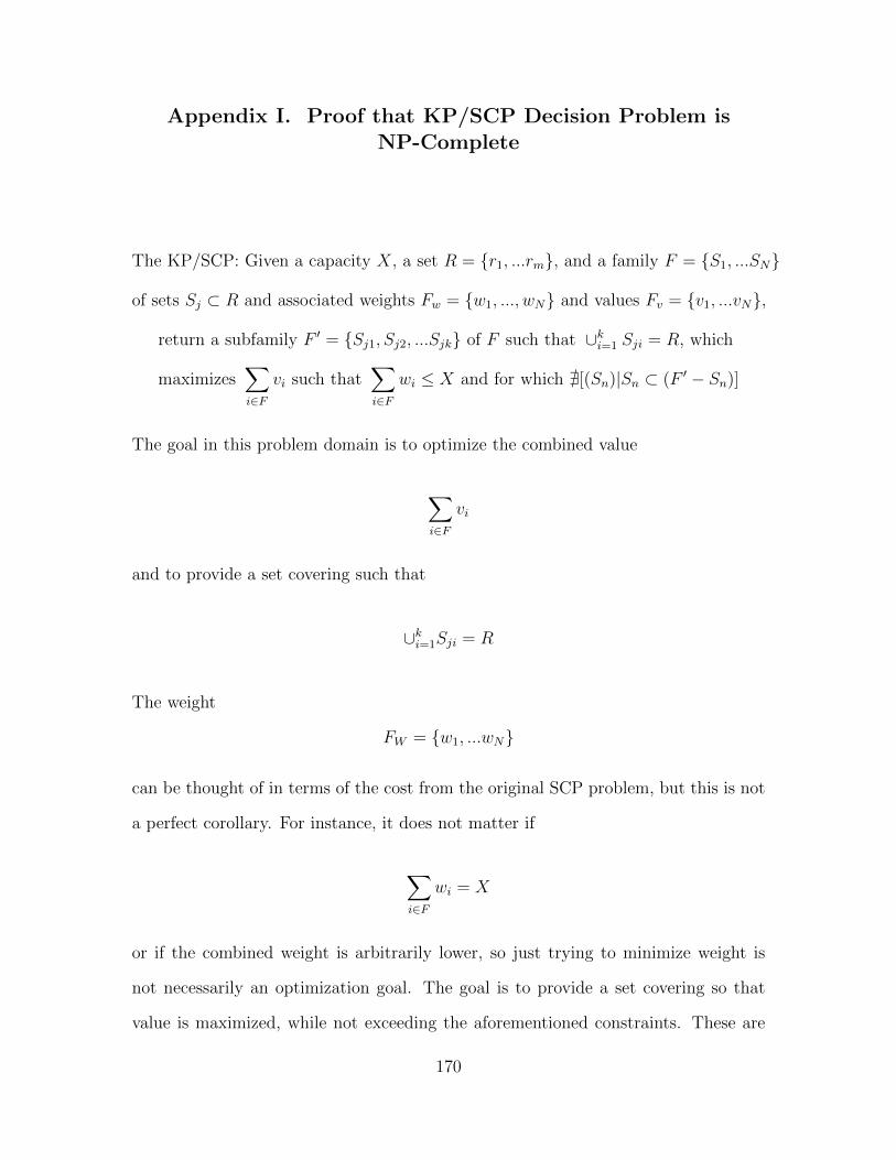
Appendix I. Proof that KP/SCP Decision Problem isNP-Complete
The KP/SCP: Given a capacity X, a set R = {r1, ...rm}, and a family F = {S1, ...SN}
of sets Sj ⊂ R and associated weights Fw = {w1, ..., wN} and values Fv = {v1, ...vN},
return a subfamily F ′ = {Sj1, Sj2, ...Sjk} of F such that ∪ki=1 Sji = R, which
maximizes∑i∈F
vi such that∑i∈F
wi ≤ X and for which @[(Sn)|Sn ⊂ (F ′ − Sn)]
The goal in this problem domain is to optimize the combined value
∑i∈F
vi
and to provide a set covering such that
∪ki=1Sji = R
The weight
FW = {w1, ...wN}
can be thought of in terms of the cost from the original SCP problem, but this is not
a perfect corollary. For instance, it does not matter if
∑i∈F
wi = X
or if the combined weight is arbitrarily lower, so just trying to minimize weight is
not necessarily an optimization goal. The goal is to provide a set covering so that
value is maximized, while not exceeding the aforementioned constraints. These are
170

competing optimizations, as there may be solutions to the Knapsack Problem which
have higher values yet which do not provide a set cover, and there may be smaller set
coverings with lower weights which provide less value.
Solution Space: Both of these problems could be solved independently if
the relevant parameters from the other problem were ignored. Even so, each is a
permutation problem, resulting in them having equivalently sized solution spaces.
Therefore this problem has a solution space of O(2n), which is the same as if they
were solved independently.
Problem Class: The KP/SCP PD can be thought of as a decision problem.
For a given answer to a SCP, is it a valid minimal set cover that meets the three
combined conditions:
Demonstrate that a decision problem has a polynomial time certifier: Proving
that the three constraints are met can be done in polynomial time:
1. Iterate through all columns and add their covered rows to a list. Check this list
against a list of required rows to confirm that they match
2. For each column, confirm that the rows which are contributed by that column
are not covered by the current solution minus that column.
3. Sum the weight of all of the items/columns and confirm that this is less than
the weight limit.
If the PD is framed as a decision problem, confirm that a given answer has a value
of at least Y.
Iterate through all items/columns and sum their values. If the summation is ≥ Y
and meets the above constraints, it is a valid answer.
The above polynomial time certifier demonstrates that the KP/SCP decision prob-
lem is NP-Complete (the full problem domain is likely NP-Hard, as it likely cannot
171

be proven that the given value of a solution is the “best” available value of the PD
in polynomial time.)
Perform a reduction from the SCP to the KP/SCP to demonstrate that the
KP/SCP decision problem is NP-Complete.
Consider a given SCP input domain. Does there exist a solution to the SCP such
that the cost is at most C?
Transform the SCP to the KP/SCP:
1. Set C to X, the maximum allowed weight
2. Set c of each column to x, the weight of each column
3. Set values v to 1. This means that the answer, though minimal from a SCP,
will not necessarily be the minimum SCP.
4. Consult the KP/SCP oracle. It will either return a family of sets that are less
than or equal to C, or will not return an answer at all.
This demonstrates that the SCP decision problem reduces to the KP/SCP. This
shows that the KP/SCP decision problem is NP-Complete. As discussed above, the
KP/SCP problem is likely NP-Hard, as it would be difficult to provide a polynomial
time certifier that a given answer is indeed optimal.
172

Bibliography
1. N. Khan, I. Yaqoob, I. A. T. Hashem, Z. Inayat, M. Ali, W. Kamaleldin, M. Alam,
M. Shiraz, and A. Gani, “Big data: survey, technologies, opportunities, and
challenges,” The Scientific World Journal, vol. 2014, 2014.
2. “Extracting business value from the 4 v’s of big data,” https://www.
ibmbigdatahub.com/infographic/extracting-business-value-4-vs-big-data, 2018.
3. C. Costa and M. Y. Santos, “Big data: state-of-the-art concepts, techniques, tech-
nologies, modeling approaches and research challenges,” IAENG International
Journal of Computer Science, vol. 43, no. 3, pp. 285–301, 2017.
4. N. Hurst, “Nathan hurst’s blog: thoughts on software, technology, and startups,”
http://blog.nahurst.com/visual-guide-to-nosql-systems, 2010.
5. P. Mathur, “Olap vs oltp,” http://olapsoftware.com/blog/olap-vs-oltp, 2013.
6. J. Abdullah, “Investigating interactive visualisation in a cloud computing envi-
ronment,” Ph.D. dissertation, Lincoln University, 2010.
7. K. Kauffman, D. Marietta, J. Kresge, M. Veth, R. Patton, J. Gray, J. Raquet,
and A. Schofield, “Field demonstration of plug and play navigation system using
scorpion and smart sensors/cables,” ION Joint Navigation Conference, 2017.
8. O. Ben-Kiki, C. Evans, and B. Ingerson, “Yaml ain’t markup language (yaml)(tm)
version 1.2,” https://yaml.org/spec/1.2/spec.html, 2009.
9. A. S. Huang, E. Olson, and D. C. Moore, “Lcm: Lightweight communications
and marshalling,” in IEEE/RSJ International Conference on Intelligent Robots
and Systems. IEEE, 2010, pp. 4057–4062.
173

10. A. S. Huang, E. Olson, and D. Moore, “Lightweight communications and mar-
shalling for low latency interprocess communication,” Computer Science and Ar-
tificial Intelligence Laboratory Technical Report, Massachusetts Institute of Tech-
nology, MA, 2009.
11. “Lcm log file format,” https://lcm-proj.github.io/log file format.html.
12. I. Yaqoob, I. A. T. Hashem, A. Gani, S. Mokhtar, E. Ahmed, N. B. Anuar, and
A. V. Vasilakos, “Big data: From beginning to future,” International Journal of
Information Management, vol. 36, no. 6, pp. 1231–1247, 2016.
13. U. Kazemi, “A survey of big data: Challenges and specifications,” CiiT Interna-
tional Journal of Software Engineering and Technology, vol. 10, no. 5, 2018.
14. F. F. Costa, “Big data in biomedicine,” Drug discovery today, vol. 19, no. 4, pp.
433–440, 2014.
15. M. Chen, S. Mao, and Y. Liu, “Big data: A survey,” Mobile networks and appli-
cations, vol. 19, no. 2, pp. 171–209, 2014.
16. J. Manyika, M. Chui, B. Brown, J. Bughin, R. Dobbs, C. Roxburgh, and A. H.
Byers, “Big data: The next frontier for innovation, competition, and productiv-
ity,” 2011.
17. S. Madden, “From databases to big data,” IEEE Internet Computing, vol. 16,
no. 3, pp. 4–6, 2012.
18. J. Anil, “The 5 v’s of big data,” https://www.ibm.com/blogs/watson-health/
the-5-vs-of-big-data/, 2016.
19. K. Krishnan, Data warehousing in the age of big data. Newnes, 2013.
174

20. P. C. Zikopoulos, C. Eaton, D. DeRoos, T. Deutsch, and G. Lapis, Understanding
big data: Analytics for enterprise class hadoop and streaming data. Mcgraw-hill
New York, 2012.
21. A. Gandomi and M. Haider, “Beyond the hype: Big data concepts, methods, and
analytics,” International Journal of Information Management, vol. 35, no. 2, pp.
137–144, 2015.
22. “What is data modeling? conceptual, logical, & physical data models,” https:
//www.guru99.com/data-modelling-conceptual-logical.html, april 2019.
23. D. Anderson, “Data model design and best practices = part 2,” https://www.
talend.com/resources/data-model-design-best-practices-part-2/, 2019.
24. P. J. Sadalage and M. Fowler, NoSQL distilled: a brief guide to the emerging
world of polyglot persistence. Pearson Education, 2013.
25. C. Li and J. Gu, “An integration approach of hybrid databases based on sql in
cloud computing environment,” Software: Practice and Experience, vol. 49, no. 3,
pp. 401–422, 2019.
26. E. F. Codd, “A relational model of data for large shared data banks,” Commu-
nications of the ACM, vol. 13, no. 6, pp. 377–387, 1970.
27. N. Jatana, S. Puri, M. Ahuja, I. Kathuria, and D. Gosain, “A survey and com-
parison of relational and non-relational database,” International Journal of En-
gineering Research & Technology, vol. 1, no. 6, pp. 1–5, 2012.
28. “Database design full course,” https://www.calebcurry.com/
freecodecamp-database-design-full-course/, 2018.
175

29. “What does acid mean in database systems,” https://database.guide/
what-is-acid-in-databases/, 2016.
30. G. Powell, Beginning database design. John Wiley & Sons, 2006.
31. C. Churcher, Beginning database design: From novice to professional. Apress,
2012.
32. S. Tuteja, “Database normalization, normal forms,” https://www.geeksforgeeks.
org/database-normalization-normal-forms/.
33. “Entity relationship diagram,” https://www.smartdraw.com/
entity-relationship-diagram/, 2019.
34. “What is entity relationship diagram,” https://www.visual-paradigm.com/
guide/data-modeling/what-is-entity-relationship-diagram/, 2019.
35. J. Kreibich, Using SQLite. O’Reilly Media, Inc., 2010.
36. “Intro to sql: Querying and managing data,” https://www.khanacademy.org/
computing/computer-programming/sql, 2019.
37. M. Dane, “Sql tutorial - full course for beginners,” https://www.youtube.com/
watch?v=HXV3zeQKqGY, 2018.
38. “Sql tutorial,” https://www.w3schools.com/sql/, 2019.
39. K. Douglas and S. Douglas, PostgreSQL, Second Edition. Sams, 2015.
40. “New to postgresql?” https://www.postgresql.org/about/, 2019.
41. A. Moniruzzaman and S. A. Hossain, “Nosql database: New era of databases for
big data analytics-classification, characteristics and comparison,” arXiv preprint
arXiv:1307.0191, 2013.
176
42. E. A. Brewer, “Towards robust distributed systems,” in PODC, vol. 7, 2000.
43. L. Perkins, E. Redmond, and J. Wilson, Seven databases in seven weeks: a guide
to modern databases and the NoSQL movement. Pragmatic Bookshelf, 2018.
44. C. Strauch, U.-L. S. Sites, and W. Kriha, “Nosql databases,” Lecture Notes,
Stuttgart Media University, vol. 20, 2011.
45. J. Cook, “Acid vs base for database transactions,” https://www.johndcook.com/
blog/2009/07/06/brewer-cap-theorem-base/, 2009.
46. R. Kune, P. K. Konugurthi, A. Agarwal, R. R. Chillarige, and R. Buyya, “The
anatomy of big data computing,” Software: Practice and Experience, vol. 46,
no. 1, pp. 79–105, 2016.
47. N. Leavitt, “Will nosql databases live up to their promise?” Computer, vol. 43,
no. 2, pp. 12–14, 2010.
48. Z. Parker, S. Poe, and S. V. Vrbsky, “Comparing nosql mongodb to an sql db,”
in Proceedings of the 51st ACM Southeast Conference. ACM, 2013, p. 5.
49. S. Chaudhuri and U. Dayal, “An overview of data warehousing and olap technol-
ogy,” ACM Sigmod record, vol. 26, no. 1, pp. 65–74, 1997.
50. B. Husemann, J. Lechtenborger, and G. Vossen, Conceptual data warehouse de-
sign. Universitat Munster. Angewandte Mathematik und Informatik, 2000.
51. G. Simsek, “What is new about newsql,” https://softwareengineeringdaily.com/
2019/02/24/what-is-new-about-newsql/, 2019.
52. “Oltp vs olap: What’s the difference?” https://www.guru99.com/oltp-vs-olap.
html, 2019.
177

53. A. Pavlo and M. Aslett, “What’s really new with newsql?” ACM Sigmod Record,
vol. 45, no. 2, pp. 45–55, 2016.
54. M. Aslett, “What we talk about when we talk about newsql,”
https://blogs.the451group.com/information management/2011/04/06/
what-we-talk-about-when-we-talk-about-newsql/, 2011.
55. W.-T. Balke and U. Guntzer, “Multi-objective query processing for database
systems,” in Proceedings of the Thirtieth international conference on Very large
data bases-Volume 30. VLDB Endowment, 2004, pp. 936–947.
56. A. Vlachou, C. Doulkeridis, K. Nørvag, and M. Vazirgiannis, “On efficient top-k
query processing in highly distributed environments,” in Proceedings of the 2008
ACM SIGMOD international conference on Management of data. ACM, 2008,
pp. 753–764.
57. S. Chaudhuri and L. Gravano, “Evaluating top-k selection queries,” in VLDB,
vol. 99, 1999, pp. 397–410.
58. E. Tiakas, A. N. Papadopoulos, and Y. Manolopoulos, “Skyline queries: An
introduction,” in 2015 6th International Conference on Information, Intelligence,
Systems and Applications (IISA). IEEE, 2015, pp. 1–6.
59. D. Kossmann, F. Ramsak, and S. Rost, “Shooting stars in the sky: An online
algorithm for skyline queries,” in Proceedings of the 28th international conference
on Very Large Data Bases. VLDB Endowment, 2002, pp. 275–286.
60. D. Papadias, Y. Tao, G. Fu, and B. Seeger, “An optimal and progressive algorithm
for skyline queries,” in Proceedings of the 2003 ACM SIGMOD international
conference on Management of data. ACM, 2003, pp. 467–478.
178

61. P. Mell and T. Grance, “Effectively and securely using the cloud computing
paradigm,” NIST, Information Technology Laboratory, vol. 2, no. 8, pp. 304–311,
2009.
62. V. Saratchandran, “Cloud service models saas, iaas, paas - choose
the right one for your business,” https://www.fingent.com/blog/
cloud-service-models-saas-iaas-paas-choose-the-right-one-for-your-business,
2018.
63. C. Gyorodi, R. Gyorodi, G. Pecherle, and A. Olah, “A comparative study: Mon-
godb vs. mysql,” in 2015 13th International Conference on Engineering of Modern
Electric Systems (EMES). IEEE, 2015, pp. 1–6.
64. I. A. T. Hashem, I. Yaqoob, N. B. Anuar, S. Mokhtar, A. Gani, and S. U. Khan,
“The rise of “big data” on cloud computing: Review and open research issues,”
Information systems, vol. 47, pp. 98–115, 2015.
65. R. Laigner, M. Kalinowski, S. Lifschitz, R. S. Monteiro, and D. de Oliveira, “A
systematic mapping of software engineering approaches to develop big data sys-
tems,” in 2018 44th Euromicro Conference on Software Engineering and Advanced
Applications (SEAA). IEEE, 2018, pp. 446–453.
66. D. Manthey, “Resonant girder,” https://tinyurl.com/yy589rof, 2019.
67. S. Mochocki, K. Kauffman, R. Leishman, and J. Racquet, “Relational database
design and multi-objective database queries for position navigation and timing
data,” Master’s thesis, Air Force Institute of Technology, 2950 Hobson Way,
Wright-Patterson AFB, OH 45433, 2020.
68. “Amazon relational database service,” https://aws.amazon.com/rds/, 2019.
179
69. “Amazon documentdb (with mongodb compatability),” https://aws.amazon.
com/documentdb/, 2019.
70. M.-G. Jung, S.-A. Youn, J. Bae, and Y.-L. Choi, “A study on data input and
output performance comparison of mongodb and postgresql in the big data envi-
ronment,” in 8th International Conference on Database Theory and Application
(DTA). IEEE, 2015, pp. 14–17.
71. A. Makris, K. Tserpes, G. Spiliopoulos, and D. Anagnostopoulos, “Performance
evaluation of mongodb and postgresql for spatio-temporal data.” in EDBT/ICDT
Workshops, 2019.
72. J. S. Van der Veen, B. Van der Waaij, and R. J. Meijer, “Sensor data storage
performance: Sql or nosql, physical or virtual,” in IEEE fifth international con-
ference on cloud computing. IEEE, 2012, pp. 431–438.
73. “Object identifier types,” https://www.postgresql.org/docs/8.1/datatype-oid.
html, 2019.
74. K. Kauffman, J. Raquet, D. Marietta, D. Carson, A. Schofield, M. Caporellie,
A. Canciani, and R. Leishman, “A modular sensor fusion approach for comple-
mentary navigation sensors,” ION Joint Navigation Conference, 2020.
75. “Class date,” https://docs.oracle.com/javase/7/docs/api/java/util/Date.html,
2018.
76. A. Caprara, P. Toth, and M. Fischetti, “Algorithms for the set covering problem,”
Annals of Operations Research, vol. 98, no. 1-4, pp. 353–371, 2000.
77. T. A. Feo and M. G. Resende, “A probabilistic heuristic for a computationally
difficult set covering problem,” Operations research letters, vol. 8, no. 2, pp. 67–
71, 1989.
180

78. J. Kleinberg and E. Tardos, Algorithm design. Pearson Education India, 2006.
79. C. Chekuri and S. Khanna, “A polynomial time approximation scheme for the
multiple knapsack problem,” SIAM Journal on Computing, vol. 35, no. 3, pp.
713–728, 2005.
80. E.-G. Talbi, Metaheuristics: from design to implementation. John Wiley & Sons,
2009, vol. 74.
81. M. Solar, V. Parada, and R. Urrutia, “A parallel genetic algorithm to solve the
set-covering problem,” Computers & Operations Research, vol. 29, no. 9, pp.
1221–1235, 2002.
82. J. E. Beasley and P. C. Chu, “A genetic algorithm for the set covering problem,”
European journal of operational research, vol. 94, no. 2, pp. 392–404, 1996.
83. J. Cobonkerr, “scp-genetic-algorithm,” https://github.com/jamescobonkerr/
scp-genetic-algorithm, 2020.
84. S. Arnborg, “Efficient algorithms for combinatorial problems on graphs with
bounded, decomposability—a survey,” Bit, vol. 25, no. 1, pp. 2–23, 1985.
85. A. A. Lazarev and F. Werner, “A graphical realization of the dynamic program-
ming method for solving np-hard combinatorial problems,” Computers & Math-
ematics with Applications, vol. 58, no. 4, pp. 619–631, 2009.
86. M. S. Krishnamoorthy, “An np-hard problem in bipartite graphs,” ACM SIGACT
News, vol. 7, no. 1, pp. 26–26, 1975.
87. M. Rosendo and A. Pozo, “Applying a discrete particle swarm optimization al-
gorithm to combinatorial problems,” in 2010 Eleventh Brazilian Symposium on
Neural Networks. IEEE, 2010, pp. 235–240.
181
88. N. Christofides, Graph theory: An algorithmic approach (Computer science and
applied mathematics). Academic Press, Inc., 1975.
89. G. Lamont, “Scp/spp global depth-first search back-tracking design,” Depart of
Electrical and Computer Engineering, Air Force Institute of Technology, 2019.
90. P. C. Chu and J. E. Beasley, “A genetic algorithm for the generalised assignment
problem,” Computers & Operations Research, vol. 24, no. 1, pp. 17–23, 1997.
91. G. Konjevod, “Solving a set covering problem with genetic algorithms1,” Max
Planck Society Technical Report MPI-I-94-604, Potsdam, 1994.
92. C. R. Reeves, “Using genetic algorithms with small populations.” in ICGA, vol.
590, 1993, p. 92.
93. A. Piszcz and T. Soule, “Genetic programming: Optimal population sizes for
varying complexity problems,” in Proceedings of the 8th annual conference on
Genetic and evolutionary computation, 2006, pp. 953–954.
182

REPORT DOCUMENTATION PAGE Form ApprovedOMB No. 0704–0188
The public reporting burden for this collection of information is estimated to average 1 hour per response, including the time for reviewing instructions, searching existing data sources, gathering andmaintaining the data needed, and completing and reviewing the collection of information. Send comments regarding this burden estimate or any other aspect of this collection of information, includingsuggestions for reducing this burden to Department of Defense, Washington Headquarters Services, Directorate for Information Operations and Reports (0704–0188), 1215 Jefferson Davis Highway,Suite 1204, Arlington, VA 22202–4302. Respondents should be aware that notwithstanding any other provision of law, no person shall be subject to any penalty for failing to comply with a collectionof information if it does not display a currently valid OMB control number. PLEASE DO NOT RETURN YOUR FORM TO THE ABOVE ADDRESS.
1. REPORT DATE (DD–MM–YYYY) 2. REPORT TYPE 3. DATES COVERED (From — To)
4. TITLE AND SUBTITLE 5a. CONTRACT NUMBER
5b. GRANT NUMBER
5c. PROGRAM ELEMENT NUMBER
5d. PROJECT NUMBER
5e. TASK NUMBER
5f. WORK UNIT NUMBER
6. AUTHOR(S)
7. PERFORMING ORGANIZATION NAME(S) AND ADDRESS(ES) 8. PERFORMING ORGANIZATION REPORTNUMBER
9. SPONSORING / MONITORING AGENCY NAME(S) AND ADDRESS(ES) 10. SPONSOR/MONITOR’S ACRONYM(S)
11. SPONSOR/MONITOR’S REPORTNUMBER(S)
12. DISTRIBUTION / AVAILABILITY STATEMENT
13. SUPPLEMENTARY NOTES
14. ABSTRACT
15. SUBJECT TERMS
16. SECURITY CLASSIFICATION OF:
a. REPORT b. ABSTRACT c. THIS PAGE
17. LIMITATION OFABSTRACT
18. NUMBEROFPAGES
19a. NAME OF RESPONSIBLE PERSON
19b. TELEPHONE NUMBER (include area code)
Standard Form 298 (Rev. 8–98)Prescribed by ANSI Std. Z39.18
26–03–2020 Master’s Thesis Sept 2019 — Mar 2020
Relational Database Design and Multi-Objective Database Queries forPosition Navigation and Timing Data
Mochocki, Sean A., Captain, USAF
Air Force Institute of TechnologyGraduate School of Engineering an Management (AFIT/EN)2950 Hobson WayWPAFB OH 45433-7765
AFIT-ENG-MS-20-M-045
Intentionally Left Blank
DISTRIBUTION STATEMENT A:APPROVED FOR PUBLIC RELEASE; DISTRIBUTION UNLIMITED.
This work is declared a work of the U.S. Government and is not subject to copyright protection in the United States.
The ANT center has access to over 100 position, navigation and timing data sets, which are stored in different formatsand locations. These data sets would be valuable to students designing filters as part of their research and could be usedto supplement physical testing, but are mostly unavailable. This thesis presents the design and testing of three possibledatabase approaches to store this PNT data in the Scorpion Data Model format. The best performing solution is thenused to test two stochastic algorithms for multi-objective database queries in the Knapsack and Set Covering problemdomains. This thesis provides valuable tools to enable future navigation research.
Relational Database, Multi-Objective Database Queries, Structured Query Language, Scorpion Data Model
U U U UU 199
Dr. Robert Leishman, AFIT/ENG
(937) 255-3636 x4755; [email protected]