Relational Query Optimization

198:541

Overview of Query Optimization

Plan: Tree of R.A. ops, with choice of alg for each op. Each operator typically implemented using a `pull’

interface: when an operator is `pulled’ for the next output tuples, it `pulls’ on its inputs and computes them.

Two main issues: For a given query, what plans are considered?

Algorithm to search plan space for cheapest (estimated) plan.

How is the cost of a plan estimated? Ideally: Want to find best plan. Practically: Avoid worst

plans! We will study the System R approach.

Highlights of System R Optimizer

Impact: Most widely used currently; works well for < 10 joins.

Cost estimation: Approximate art at best. Statistics, maintained in system catalogs, used to

estimate cost of operations and result sizes. Considers combination of CPU and I/O costs.

Plan Space: Too large, must be pruned. Only the space of left-deep plans is considered.

Left-deep plans allow output of each operator to be pipelined into the next operator without storing it in a temporary relation.

Cartesian products avoided.

Schema for Examples

Similar to old schema; rname added for variations.

Reserves: Each tuple is 40 bytes long, 100 tuples per page,

1000 pages. Sailors:

Each tuple is 50 bytes long, 80 tuples per page, 500 pages.

Sailors (sid: integer, sname: string, rating: integer, age: real)Reserves (sid: integer, bid: integer, day: dates, rname: string)

Motivating Example

Cost: 1000+1000*500 I/Os By no means the worst plan! Misses several opportunities:

selections could have been `pushed’ earlier, no use is made of any available indexes, etc.

Goal of optimization: To find more efficient plans that compute the same answer.

SELECT S.snameFROM Reserves R, Sailors SWHERE R.sid=S.sid AND R.bid=100 AND S.rating>5

Reserves Sailors

sid=sid

bid=100 rating > 5

sname

Reserves Sailors

sid=sid

bid=100 rating > 5

sname

(Simple Nested Loops)

(On-the-fly)

(On-the-fly)

RA Tree:

Plan:

Alternative Plans 1 (No Indexes)

Main difference: push selects. With 5 buffers, cost of plan:

Scan Reserves (1000) + write temp T1 (10 pages, if we have 100 boats, uniform distribution).

Scan Sailors (500) + write temp T2 (250 pages, if we have 10 ratings).

Sort T1 (2*2*10), sort T2 (2*3*250), merge (10+250) Total: 3560 page I/Os.

If we used BNL join, join cost = 10+4*250, total cost = 2770. If we `push’ projections, T1 has only sid, T2 only sid and

sname: T1 fits in 3 pages, cost of BNL drops to under 250 pages, total <

2000.

Reserves Sailors

sid=sid

bid=100

sname(On-the-fly)

rating > 5(Scan;write to temp T1)

(Scan;write totemp T2)

(Sort-Merge Join)

Alternative Plans 2With Indexes

With clustered index on bid of Reserves, we get 100,000/100 = 1000 tuples on 1000/100 = 10 pages.

INL with pipelining (outer is not materialized).

Decision not to push rating>5 before the join is based on availability of sid index on Sailors. Cost: Selection of Reserves tuples (10 I/Os); for each, must get matching Sailors tuple (1000*1.2); total 1210 I/Os.

Join column sid is a key for Sailors.–At most one matching tuple, unclustered index on sid OK.

–Projecting out unnecessary fields from outer doesn’t help.

Reserves

Sailors

sid=sid

bid=100

sname(On-the-fly)

rating > 5

(Use hashindex; donot writeresult to temp)

(Index Nested Loops,with pipelining )

(On-the-fly)

Query Blocks: Units of Optimization

An SQL query is parsed into a collection of query blocks, and these are optimized one block at a time.

Nested blocks are usually treated as calls to a subroutine, made once per outer tuple. (This is an over-simplification, but serves for now.)

SELECT S.snameFROM Sailors SWHERE S.age IN (SELECT MAX (S2.age) FROM Sailors S2 GROUP BY S2.rating)

Nested blockOuter block

For each block, the plans considered are:– All available access methods, for each reln in FROM clause.– All left-deep join trees (i.e., all ways to join the relations one-at-a-time, with the inner reln in the FROM clause, considering all reln permutations and join methods.)

Cost Estimation

For each plan considered, must estimate cost: Must estimate cost of each operation in plan tree.

Depends on input cardinalities. We’ve already discussed how to estimate the cost of

operations (sequential scan, index scan, joins, etc.) Must estimate size of result for each operation in tree!

Use information about the input relations. For selections and joins, assume independence of

predicates. We’ll discuss the System R cost estimation approach.

Very inexact, but works ok in practice. More sophisticated techniques known now.

Statistics and Catalogs

Need information about the relations and indexes involved. Catalogs typically contain at least: # tuples (NTuples) and # pages (NPages) for each

relation. # distinct key values (NKeys) and NPages for each index. Index height, low/high key values (Low/High) for each tree

index. Catalogs updated periodically.

Updating whenever data changes is too expensive; lots of approximation anyway, so slight inconsistency ok.

More detailed information (e.g., histograms of the values in some field) are sometimes stored.

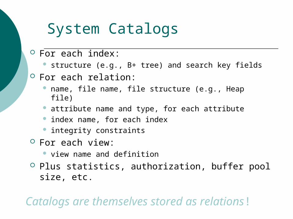
System Catalogs

For each index: structure (e.g., B+ tree) and search key fields

For each relation: name, file name, file structure (e.g., Heap file) attribute name and type, for each attribute index name, for each index integrity constraints

For each view: view name and definition

Plus statistics, authorization, buffer pool size, etc.

Catalogs are themselves stored as relations!

Attr_Cat(attr_name, rel_name, type, position)

attr_name rel_name type positionattr_name Attribute_Cat string 1rel_name Attribute_Cat string 2type Attribute_Cat string 3position Attribute_Cat integer 4sid Students string 1name Students string 2login Students string 3age Students integer 4gpa Students real 5fid Faculty string 1fname Faculty string 2sal Faculty real 3

Size Estimation and Reduction Factors

Consider a query block: Maximum # tuples in result is the product of the

cardinalities of relations in the FROM clause. Reduction factor (RF) associated with each term reflects

the impact of the term in reducing result size. Result cardinality = Max # tuples * product of all RF’s. Implicit assumption that terms are independent! Term col=value has RF 1/NKeys(I), given index I on col Term col1=col2 has RF 1/MAX(NKeys(I1), NKeys(I2)) Term col>value has RF (High(I)-value)/(High(I)-Low(I))

SELECT attribute listFROM relation listWHERE term1 AND ... AND termk

Relational Algebra Equivalences

Allow us to choose different join orders and to `push’ selections and projections ahead of joins.

Selections: c cn c cnR R1 1 ... . . .

c c c cR R1 2 2 1 (Commute)

Projections: a a anR R1 1 . . . (Cascade)

Joins: R (S T) (R S) T (Associative)

(R S) (S R) (Commute)

(Cascade)

More Equivalences

A projection commutes with a selection that only uses attributes retained by the projection.

Selection between attributes of the two arguments of a cross-product converts cross-product to a join.

A selection on just attributes of R commutes with R S. (i.e., (R S) (R) S )

Similarly, if a projection follows a join R S, we can `push’ it by retaining only attributes of R (and S) that are needed for the join or are kept by the projection.

Enumeration of Alternative Plans

There are two main cases: Single-relation plans Multiple-relation plans

For queries over a single relation, queries consist of a combination of selects, projects, and aggregate ops: Each available access path (file scan / index) is

considered, and the one with the least estimated cost is chosen.

The different operations are essentially carried out together (e.g., if an index is used for a selection, projection is done for each retrieved tuple, and the resulting tuples are pipelined into the aggregate computation).

Cost Estimates for Single-Relation Plans

Index I on primary key matches selection: Cost is Height(I)+1 for a B+ tree, about 1.2 for hash

index. Clustered index I matching one or more selects:

(NPages(I)+NPages(R)) * product of RF’s of matching selects.

Non-clustered index I matching one or more selects: (NPages(I)+NTuples(R)) * product of RF’s of matching

selects. Sequential scan of file:

NPages(R). Note: Typically, no duplicate elimination on

projections! (Exception: Done on answers if user says DISTINCT.)

Example

If we have an index on rating: (1/NKeys(I)) * NTuples(R) = (1/10) * 40000 tuples

retrieved. Clustered index: (1/NKeys(I)) * (NPages(I)+NPages(R)) =

(1/10) * (50+500) pages are retrieved. (This is the cost.) Unclustered index: (1/NKeys(I)) * (NPages(I)

+NTuples(R)) = (1/10) * (50+40000) pages are retrieved.

If we have an index on sid: Would have to retrieve all tuples/pages. With a

clustered index, the cost is 50+500, with unclustered index, 50+40000.

Doing a file scan: We retrieve all file pages (500).

SELECT S.sidFROM Sailors SWHERE S.rating=8

Queries Over Multiple Relations

Fundamental decision in System R: only left-deep join trees are considered. As the number of joins increases, the number of alternative

plans grows rapidly; we need to restrict the search space. Left-deep trees allow us to generate all fully pipelined plans.

Intermediate results not written to temporary files. Not all left-deep trees are fully pipelined (e.g., SM

join).

BA

C

D

BA

C

D

C DBA

Enumeration of Left-Deep Plans

Left-deep plans differ only in the order of relations, the access method for each relation, and the join method for each join.

Enumerated using N passes (if N relations joined): Pass 1: Find best 1-relation plan for each relation. Pass 2: Find best way to join result of each 1-relation plan

(as outer) to another relation. (All 2-relation plans.) Pass N: Find best way to join result of a (N-1)-relation plan

(as outer) to the N’th relation. (All N-relation plans.) For each subset of relations, retain only:

Cheapest plan overall, plus Cheapest plan for each interesting order of the tuples.

Enumeration of Plans (Contd.)

ORDER BY, GROUP BY, aggregates etc. handled as a final step, using either an `interestingly ordered’ plan or an addtional sorting operator.

An N-1 way plan is not combined with an additional relation unless there is a join condition between them, unless all predicates in WHERE have been used up. i.e., avoid Cartesian products if possible.

In spite of pruning plan space, this approach is still exponential in the # of tables.

Cost Estimation for Multirelation Plans

Consider a query block: Maximum # tuples in result is the product of the

cardinalities of relations in the FROM clause. Reduction factor (RF) associated with each term

reflects the impact of the term in reducing result size. Result cardinality = Max # tuples * product of all RF’s.

Multirelation plans are built up by joining one new relation at a time. Cost of join method, plus estimation of join

cardinality gives us both cost estimate and result size estimate

SELECT attribute listFROM relation listWHERE term1 AND ... AND termk

Example Pass1:

Sailors: B+ tree matches rating>5, and is probably cheapest. However, if this selection is expected to retrieve a lot of tuples, and index is unclustered, file scan may be cheaper.

Still, B+ tree plan kept (because tuples are in rating order).

Reserves: B+ tree on bid matches bid=100; cheapest.

Sailors: B+ tree on rating Hash on sidReserves: B+ tree on bid

Pass 2:– We consider each plan retained from Pass 1 as the outer, and consider how to join it with the (only) other relation.

e.g., Reserves as outer: Hash index can be used to get Sailors tuples that satisfy sid = outer tuple’s sid value.

Reserves Sailors

sid=sid

bid=100 rating > 5

sname

Nested Queries

Nested block is optimized independently, with the outer tuple considered as providing a selection condition.

Outer block is optimized with the cost of `calling’ nested block computation taken into account.

Implicit ordering of these blocks means that some good strategies are not considered. The non-nested version of the query is typically optimized better.

SELECT S.snameFROM Sailors SWHERE EXISTS (SELECT * FROM Reserves R WHERE R.bid=103 AND R.sid=S.sid)

Nested block to optimize: SELECT * FROM Reserves R WHERE R.bid=103 AND S.sid= outer valueEquivalent non-nested query:

SELECT S.snameFROM Sailors S, Reserves RWHERE S.sid=R.sid AND R.bid=103

Summary

Query optimization is an important task in a relational DBMS.

Must understand optimization in order to understand the performance impact of a given database design (relations, indexes) on a workload (set of queries).

Two parts to optimizing a query: Consider a set of alternative plans.

Must prune search space; typically, left-deep plans only. Must estimate cost of each plan that is considered.

Must estimate size of result and cost for each plan node. Key issues: Statistics, indexes, operator implementations.

Summary (Contd.)

Single-relation queries: All access paths considered, cheapest is chosen. Issues: Selections that match index, whether index key has

all needed fields and/or provides tuples in a desired order. Multiple-relation queries:

All single-relation plans are first enumerated. Selections/projections considered as early as possible.

Next, for each 1-relation plan, all ways of joining another relation (as inner) are considered.

Next, for each 2-relation plan that is `retained’, all ways of joining another relation (as inner) are considered, etc.

At each level, for each subset of relations, only best plan for each interesting order of tuples is `retained’.