Abstract— Generalization is one of the most challenging issues

of Learning Classifier Systems. This feature depends on the representation method which the system used. Considering the proposed representation schemes for Learning Classifier System, it can be concluded that many of them are designed to describe the shape of the region which the environmental states belong and the other relations of the environmental state with that region was ignored. In this paper, we propose a new representation scheme which is designed to show various relationships between the environmental state and the region that is specified with a particular classifier.

Keywords—Classifier Systems, Reinforcement Learning, Relational Representation, XCSF.

I. INTRODUCTION NE of the most important goals in Learning Classifier Systems [1] is to achieve a compact and accurate solution

for a given problem. This feature depends on the representation method which the system used. Learning Classifier Systems such as XCS [2], traditionally use binary representation. The other extensions to XCS such as XCSF [3] use other representations such as ternary [4], interval [5], ellipsoids [6], and convex hull [7]. Considering the proposed representation schemes for Learning Classifier System, we can conclude that many of them are designed to describe the shape of the region which the environmental states belong and other relations of the environmental state with that region was ignored.

Our main contribution in this paper is to propose a new representation scheme for XCSF. This scheme is designed to show the other relationships in addition to the inclusion relation between the environmental state and the region that is specified with a particular classifier. We call this representation Relational Condition Representation.

The rest of this paper is organized as follows: at first, we briefly describe XCSF, and then we summarize some important works about representation issues in XCSF. After that, we describe our proposed scheme in details. Finally, the benchmark problems are introduced and the experimental results are described and discussed.

M. A. Tabarzad is with the Center of Excellence: Control and Intelligent

Processing, University of Tehran, Tehran, Iran (phone: +98-021-88027757; fax: +98-021-88633029; e-mail: m.tabarzad@ ece.ut.ac.ir).

C. Lucas is with the Center of Excellence: Control and Intelligent Processing, University of Tehran, Tehran, Iran and School of Cognitive Sciences, IPM, Iran(e-mail: lucas@ipm.ir).

A. Hamzeh is with the Computer Engineering Department, Iran University of Science and Technology, Tehran, Iran (e-mail: hamzeh@iust.ac.ir).

II. XCSF IN BRIEF XCSF [3] is a newly introduced model of XCS that is able to compute the classifiers prediction instead of memorizing them. To do so, the original XCS is modified in three concepts: (i) Classifier conditions are modified to accept numerical inputs. (ii) A weight vector is added to each classifier to compute the predicted reward and (iii) the update procedure of XCS was changed to involve the weight vector in the update process. These modifications are described in the following: In XCSF, each classifier has a condition and an action. The condition consists of an interval in the form of (li, ui) which matches the environmental inputs between li (the lower bound) and ui (the upper bound) and the action is as same as the original XCS. Also there exist four other parameters associated with each classifier: the weight vector (W), the prediction reward error (ε) the fitness f and the numerosity num. the f, ε and num are as same as XCS and are used to determine the accuracy of each classifier, the error occurred during the reward prediction procedure, and the number of micro-classifiers in the related macro-classifier. The weight vector W is used to compute the classifier predicted rewards as a function of the current environmental input. This vector has one weight w1 for each possible input and an additional weight w0 for a constant input x0 that is set in the initialization phase of the XCSF. In the learning phase of XCSF, in each time step t, XCSF, as same as XCS, builds a match set [M] containing some classifiers in the population [P] that match the input st, which determines the current environmental state. If the number of distinct actions in the [M] was less than a threshold θmna, then the covering operator creates a new classifier that matches st with an action differs from the actions in [M]. This process continues till the number of the distinct actions in [M] reaches the θmna. Then for each action ai in [M], XCSF calculates the estimated payoff of the system in the case of applying action ai to the environment. But in contrast with XCS, in XCSF the predicted reward is calculated using equation 1.

where cl is a matching classifier in [M] which its action is a, cl.F is the fitness of that classifier and cl.p is its prediction which is calculated using equation 2.

Relational Representation in XCSF Mohammad Ali Tabarzad, Caro Lucas, and Ali Hamzeh

O

[ ]

[ ]∑∑

∈

∈×

=aMcl

aMcl tt Fcl

FclspclasP

|

|

.

.)(.),(

(1)

)(..)(.0

00 iswclxwclspcli

tit ∑>

×+×=

(2)

where cl.wi, is the iTh element of the vector W of cl and x0 is the described constant input. Then XCSF selects an action to perform, respecting its policy to explore or exploit the environment. Then all classifiers in [M] with the same action are selected and inserted into [A]. Then this action is applied to the environment and the reward r is fed back to the system. Note that in our experiments for function approximation, there exists only one dummy action which has no actual effect on the system. However, the reward r is used to update the associated parameters of the classifiers in [A]. To do so, the weight vectors W are updated using a modified delta rule [8] for all classifiers in [A]. To update the corresponding weight vector, each wi is updated using a Δwi which is computed as follows:

)())(.( 1121

iXsoclrX

w ttt

i −−

−

−=Δη

(3)

where η is the correction rate and Xt-1 is the associated input vector for the previous state st-1 and |Xt-1|2 is the normal vector of Xt-1. Then each classifier weight is updated as follows:

iii wwclwcl Δ+← .. (4)

Also the predicted rewards error ε is updated as:

).)(.(.. 1 εβεε clspclrclcl t −−+← − (5)

Then classifier fitness is updated using the relational accuracy of a classifier. To do so, the raw accuracy is computed as follows:

Then, the relational accuracy is computed using equation 7.

[ ]∑ ∈×

×=

Aclnumclcl

num)..(

'κ

κκ

(7)

where cl.κ is the raw accuracy of the classifier and cl.num is the numerosity of classifier cl. Then the relative accuracy κ’ is used to update the classifier fitness as follows: )'( FFF −+← κβ . An algorithmic description of the overall update procedure is reported in [9].

III. RELATED WORKS ON CONDITION REPRESENTATION FOR REAL NUMBERS IN CLASSIFIER SYSTEMS

In this section, we summarize some of the most important works about condition representation for real numbers in XCSF.

In [10], the author introduced an extension to XCS called XCSR. The aim of this extension is to handle real valued input parameter. To do so, XCSR uses a center-radiant tuple to

represent a desired interval. This representation was the first one that is used in the area of real valued XCSs.

In [5], the author modified XCSR [10] to introduce the interval-based representation. This new representation used a lower-upper bound tuple. This representation is the current representation in the XCSF and any other extension to XCS with the ability to handle real valued input parameters.

In [11], the authors analyzed two interval-based representations which are commonly used in XCS. They proved with sufficient evidences that there exist a bias in representational methods and used operators. They proposed a new interval-based representation. They also proposed a new test problem which can be used to determine wheatear there exist bias or not.

In [6], the author proposed a new representational scheme based on hyper-spheres and hyper-ellipsoids. It was shown that their suggested presentations methods improved performance in continuous functions.

And at last in [7], the authors introduced a representation of classifier conditions based on the convex hull. In this kind of representation a set of points in the problem is used to identify a convex hull to determine the problem space. They applied their version of XCSF to function approximation problems and compared its performance to the original XCSF.

IV. THE RELATIONAL REPRESENTATION Considering the described representation schemes, we can

say that these schemes are designed to describe the shape of the region that the environmental states belong and the other relations of the environmental state with that region are ignored. For example, no scheme was proposed to represent a classifier which covers the environmental states that do not be included in a specified region or are close to it, far from it or relates using any other similar relations with a region. In the other words, it can be concluded that the only implicit relation that is represented in the classifier’s structure is inclusion relation and the other ones are not tried yet. So, our main contribution in this paper is to propose a new representation scheme for XCSF which is designed to show the other relationships in addition to the inclusion relation between the environmental state and the region that is specified by a particular classifier. This representation is called Relational Condition Representation (RCR). In RCR, the condition part of a classifier consists of two subsections. The first one is specified to represent the relation between the environmental states and the region that is specified by the classifier and the second part is responsible to specify the region itself. The first subsection in RCR can be represented and interpreted in many different ways to represent some crisp or fuzzy relation(s) between the state and the specified region. In this paper, we use a binary representation that represents some crisp relations. This subsection is consists of two bits (b0b1) from alphabet {0, 1} that are interpreted as follows: IN the Region (00), OUT of the Region (01), CLOSE to the Region (10) and FAR From the Region (11). The interpretation scheme of these relations is described later in more details. Also, to represent the second subsection we can choose any of the

⎩⎨⎧ ≤

=− .)/(

1

0

0

otherwise

ifvεεα

εεκ

(6)

existing schemes that are proposed yet to represent the classifier’s condition in XCSF. However, we choose the interval based representation that is a commonly used representation scheme in XCSF. In this type of representation, the classifier’s condition is represented as follows:

><><>< nn ululul ,,...,,,, 2211

(8) where li and ui are the lower and the upper bound of the ith

axis. So, the classifiers in RCR are represented as follows:

actionulululbb nn },,,...,,,,,{ 221110 ><><>< (9) Due to the changes in the classifier’s representation, we

must introduce a new mechanism for the involved operators such as Matching, Covering, GA and Subsumption Deletion. These operators are as follows:

Matching: In RCR, this operator must act with respect not only to the region that is specified by the current classifier but also with respect to the relation that was stated by the ‘b0b1’ part of the classifier. So, matching state S that is indicated by a vector ‘ >< nsss ,...,, 21 ‘against the classifier C that is indicated by

‘ actionulululbb nn },,,...,,,,,{ 221110 ><><>< ’ must be done

with respect to b0b1 in the following manner: b0=0, b1=0 (IN): This relation in an implicit relation that

exists in the other representation schemes for XCSF. It means that S matches against C iff:

iiini usl <≤∀ < , (10) b0=0, b1=1 (OUT): This relation is the opposite relation of

the first one. In this case, S matches against C iff:

iiiini suorls ≤<∃ < , (11) b0=1, b1=0 (CLOSE): This relation could be interpreted in

many different ways using fuzzy or crisp context or using some other relations that are used in [6]. But in this paper, we use a very simple scheme to describe this relation. To match S against C, at first we must calculate the center of the region specified by C using (12).

2, ii

iniulc +

=∀ < (12)

Then, we calculate the distance between S and c. if this

distance is less than a predefined threshold Tc, then S matches against C.

b0=1, b1=1 (FAR): This relation is very similar to the CLOSE relation only with one difference. After calculating the distance, if it is greater than a predefined threshold Tf, then S matches against C.

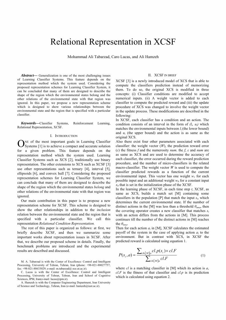
Covering: When covering occurs, the system must generate a classifier which covers the current environmental state. To do so, the system generates a sequence of random numbers as l1, u1, l2, u2, ..., ln, un. Then the current environmental state (S) is compared against the generated region using the following method:

If S lays in the region, then the new classifier is constructed using the above region and the relation will be set to IN. Otherwise, if the distance between S and the center of the region is less than Tc, then the new classifier is constructed using the above region and the relation will be set to CLOSE. Otherwise, if the distance between S and the center of the region is less than Tf, then the new classifier is constructed using the above region and the relation can only be set to OUT. Because S is not far from that region and,

Otherwise, the classifier is constructed using the above region and the relation is chosen with the probability of 0.5 between OUT or FAR.

Fig. 1 an Example of the mentioned relations

Discovery Component: for RCR representation, the genetic algorithm works as usual except the crossover and the mutation operators. The crossover is done separately on both region indicator part and the relation indicator part. The first one is as same as XCSF and the later is done using the one-point crossover operator. Also, the mutation is applied on both parts separately. In the region indicator part it is done as same as XCSF and in the relation indicator part it is done using a Pmr probability which tell the operator to change a bit of the relation part (which is selected randomly) from 0 to 1 or vice versa.

Subsumption Deletion: For subsumption deletion, we must determine whether a specified condition (C1) covers another condition (C2) or not. To do so, first the two corresponding regions R1 and R2 are considered; then the region R for 21 RR ∪ is computed; if R is equal to R1, then C1 will be more general than C2; if R is equal to R2, then C2 will be more general than C1; otherwise none of the two conditions is more general than the other one.

V. DESIGN OF THE EXPERIMENTS In our experiments, we apply XCSF to function approximation problems using the standard experimental design used in the literature [12]. Each experiment includes limited number of trials. Each trial is either a learning trial or a test trial. In learning trials, the system chooses its winner

action at random but in test trials, the winner action is chosen with respect its prediction. The internal GA is enabled only during learning trials. The covering operator is always enabled. In function approximation problems, an input tuple <x, y> and its relevant output f(x, y) is randomly selected from the problem domain. The system is expected to compute the approximated value f’(x, y) then the environment returns a reward equal to f(x, y) to the system.

A. Benchmark Problems Our used benchmark problems are categorized into two

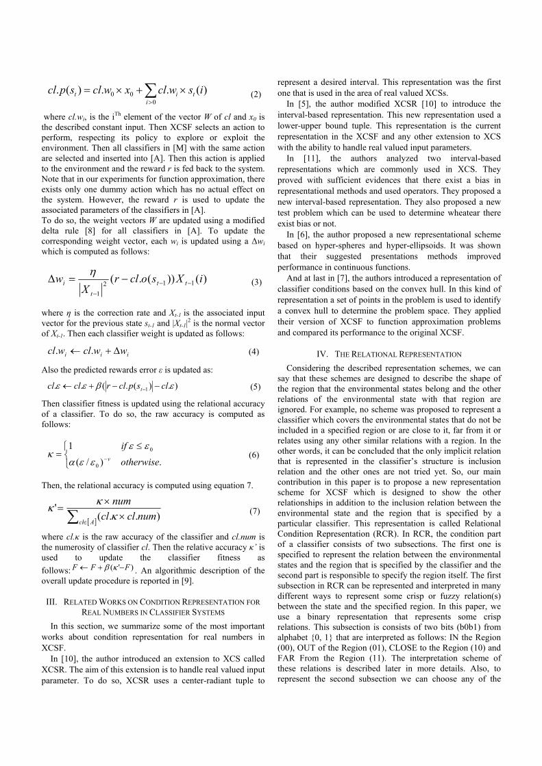
families: Grid simulated and relational simulated. To design the first family, we considered a 10*10 grid where its horizontal axis stands for x and the vertical axis stands for y. The blocks of the grid is colored as black if the value of the block is 0, gray if the value of block is 1 and white if the value of the block is 2. For example consider Fig. 2.

Fig. 2 an Example of the grid benchmark problems

It is interpreted as follows:

⎩⎨⎧

==<<<<

208.03.0,5.03.0

fotherwisefyx (13)

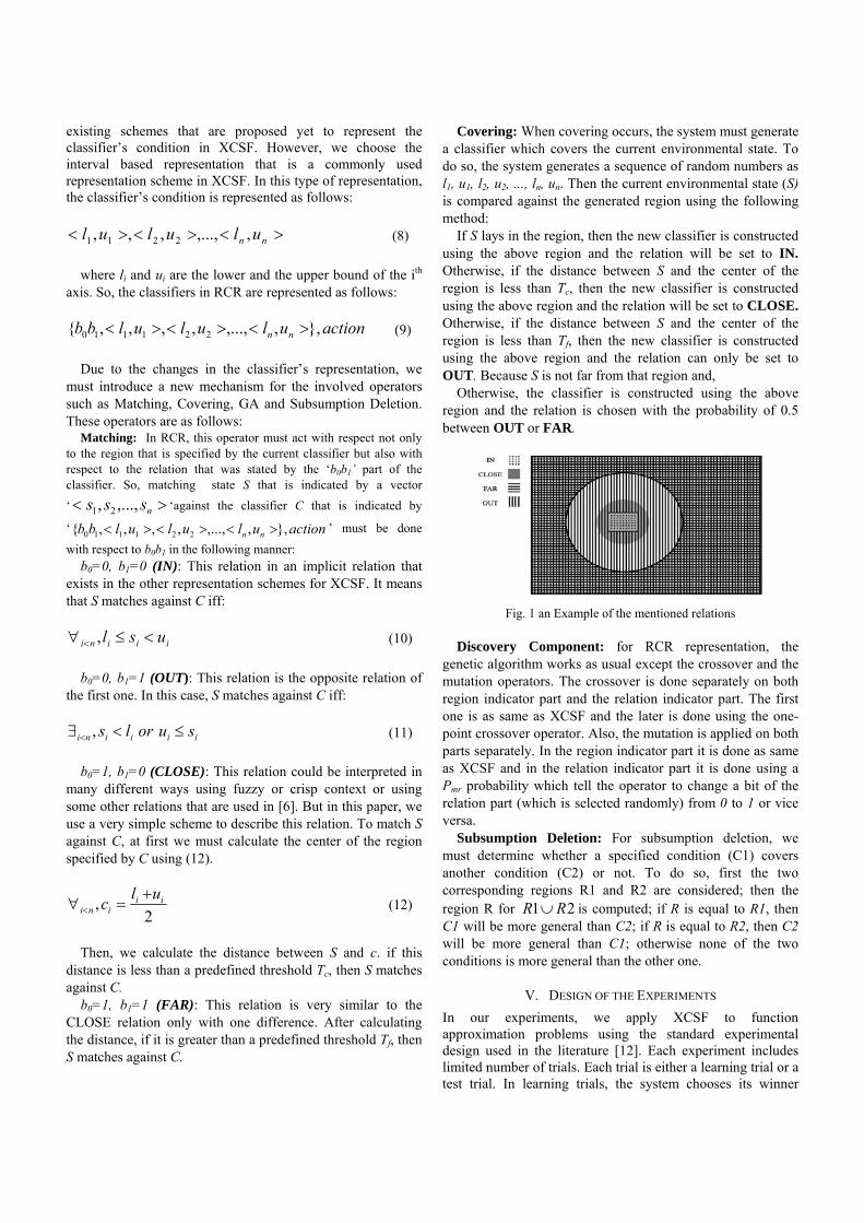
In this paper, we use three benchmark problems of this

category which are depicted in the Fig. 3.

Fig. 3 First Category of Benchmark Problems

The second type of the benchmark problems is designed with respect to the relation between x and y. it is the Frog problem and is described in the following.

The Frog Problem [12]: This function is defined as the

optimal action value. “It is basically a tent that stretches diagonally between point <0, 1> and point <1, 0>” [12] and is defined in (14).

⎩⎨⎧

>++−≤++

1)(21

yxifyxyxifyx (14)

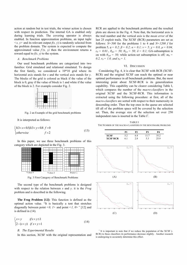
B. The Experimental Results In this section, XCSF with the original representation and

RCR are applied to the benchmark problems and the resulted plots are shown in the Fig. 4. Note that, the horizontal axis is the trail number and the vertical axis is the mean error of the last 25 exploit trails. The XCSF (RCR) parameters are set as follows: N=500 for the problems 1 to 4 and N=1200 f for problem 5, η = 0.2; β = 0.2; α = 0.1; ν = 5; χ = 0.8, µ = 0.04, ε0 = 0.01., θdel = 50; θGA = 50; δ = 0.1; GA-subsumption is on with θsub = 50; while action-set subsumption is off; m0 = 0.2, r0 = 1.0, and x0 = 1.

VI. DISCUSSION Considering Fig. 4, it is clear that XCSF with RCR (XCSF-

RCR) and the original XCSF can reach the optimal or near optimal performance in all benchmark problems. But, the most interesting point about XCSF-RCR is its generalization capability. This capability can be clearer considering Table I, which compares the number of the macro-classifiers in the original XCSF and the XCSF-RCR. This information is extracted using the following procedure: at first, all of the macro-classifiers are sorted with respect to their numerosity in descending order. Then the top ones in the queue are selected till all of the problem space will be covered by the selection set. Then, the average size of the selection set over 250 independent runs is inserted in the Table I1.

TABLE I

THE NUMBER OF THE MACRO-CLASSIFIERS IN THE BENCHMARK PROBLEMS

P1 P2 P3 P4 XCSF 5.2 6.4 11.7 35.2 XCSF RCR 6.1 2.8 5.3 25.9

(A)

(B)

(C)

(D)

1 It is important to note that if we reduce the population of the XCSF (-

RCR) to these classifiers its performance decrease slightly. Another research is undergoing to accurately determine this effect.

Fig 4 Comparing Performance of the traditional XCSF and XCSF-RCR in P1 (A), P2 (B), P3(C), and the Frog Problem (D) where XCSF-RCR is the dashed line and XCSF is the solid line. The horizontal axis is the trial number and the Vertical Axis is Error.

With respect to this table, we can say that XCSF-RCR is able to generate a more compact population than the original XCSF. This conclusion can be confirmed by a closer look to the classification results of the original XCSF and the XCSF-RCR To do so, see Fig. 5 and 6. Considering these figures, it is obvious that due to the existence of ‘out’ relation, XCSF-RCR can cover a region with an unbounded form with just one classifier. But, XCSF needs to find more classifiers to cover the same region because of the implicit inclusion relation which exists in its representation scheme. Hence, we can conclude that, the relational condition representation has the ability to describe some shapes which can not be represented with the commonly proposed scheme of representation for XCS*. It is important to note that we propose only the high level description of RCR and it can be implemented in many various ways which includes implementing other relations or modifying the current definitions of the used relations using fuzzy or crisp concepts. It seems that the RCR representation of a classifier is a powerful and extendable scheme which gives us the ability to describe the environment in a more compact manner. To quantify these results and to test whether it is statistically significant we apply these experiments 150 times with different random generators independently and then apply one-tailed Wilcoxon signed rank test [13] on the size of the resulted macro-classifier, that is measured as described before) in XCSF and XCSF-RCR. With respect to the definition of the P-Values in Wilcoxon test, we can conclude that XCSF-RCR can significantly improve the generalization capability of XCSF especially in the problems that are similar to the problems 2 and 3.

TABLE II THE RESULT OF APPLYING WILCOXON TEST ON THE DEPICTED RESULTS IN

TABLE I

Problem P1 P2 P3 P4 P(WXCSF-RCR>wXCSF-RCR) 0.379 0.023 0.042 0.256

So, it can be concluded that the shape description is a very

important feature that can improve the generalization capability of XCSF but adding other relations except the inclusion relation to the condition of the classifiers in XCSF can improve the generalization capability of the system. It the other hand, it can be a question that does this ability makes some trouble for XCSF-RCR to solve ordinary problems (which are describable with ordinary shapes such as P1)? To answer this question, we design some ordinary benchmark problems that are depicted in Fig. 7. To compare the performance of XCSF and XCSF-RCR in these ordinary problems, we introduce a new performance measuring criteria in addition to the number of the macro-classifiers that used before. This new criteria is called Optimal Reach Point (ORP). ORP is the first point that the mean performance of the system in its previous 100 iterations is equal to the OptimalValue±ε0.

Note that in these benchmark problems, the performance is measured using MAE, and the optimal value of MAE is 0. So OPR is the first point that the mean MAE of the system in the previous 100 iterations is less that ε0, where ε0 is set to 0.01 in this research.

Fig. 5 Classification of the problem 2 by XCSF

(A) and XCSF-RCR (B)

Fig. 6 Classification of the problem 3 by XCSF

(A) and XCSF-RCR (B)

With respect to Table III, we can conclude that adding the relational representation capability to XCSF has no significant effect on its ability to solve ordinary problems. To confirm this conclusion, consider Table IV.

Fig. 7 Ordinary Benchmark Problems

TABLE III THE RESULTS OF APPLYING XCSF AND XCSF-RCR ON PO1, PO2 AND PO3

(AVERAGED OVER 25 INDEPENDENT RUNS)

PO1 PO2 PO3 ORP XCSF 1782 751 2941

XCSF-RCR 1830 732 3052

TABLE IV

THE RESULTS OF APPLYING THE WICOXON TEST ON THE NUMBER OF THE MACRO-CLASSIFIERS IN THE BENCHMARK PROBLEMS

Problem PO1 PO2 PO3

XCSF vs. XCSF-RCR 0.832 0.745 0.669

VII. SUMMARY In this paper, we propose a new representation scheme for

XCSF, which is based on representing different relationships

between the environmental states and the region that is specified by a classifier. These relations can be chosen in many different ways using crisp or fuzzy context and are going to replace the implicit inclusion relation in the other representation scheme. Our proposed scheme is called Relational Condition Representation (RCR) and is applied on some benchmark problems and is compared with the original XCSF. The experimental results showed that this scheme can improves XCSF’s compactness of the population. Finally, we can say that this type of representation, can improve the generalization capability of the XCSF. Finally, it can be concluded that adding relational representation feature to XCSF can improve its generalization capability in problems with unbounded class definition (e.g. P2, P3) and has no significant effect on the performance of XCSF in ordinary problems (e.g. Frog and P1)

REFERENCES [1] J.H. Holland, 1986, Escaping Brittleness: The Possibilities of General-

Purpose Learning Algorithms Applied to Parallel Rule-Based Systems, Machine Learning: An Artificial Intelligence Approach, Volume II, Michalski, Ryszard S., Carbonell, Jamie G., and Mitchell, Tom M. (eds.), Morgan Kaufman Publishers, Inc., Los Altos, CA.

[2] S. W. Wilson, 1995, Classifier Fitness Based on Accuracy, Evolutionary Computation, 3(2):149–175.

[3] S.W. Wilson, 2001, Function Approximation with a Classifier System, In proceedings of the Genetic and Evolutionary Computation Conference (GECCO-2001), San Francisco, California, USA, pp. 974-981. Morgan Kaufmann.

[4] P. L. Lanzi, D. Loiacono, S. W. Wilson, and D. E. Goldberg, 2005, XCS with Computed Prediction for the Learning of Boolean Functions, In Proceedings of the IEEE Congress on Evolutionary Computation – CEC-2005, Edinburgh, UK.

[5] S. W. Wilson, 1996, Mining Oblique Data with XCS, volume 1996 of Lecture notes in Computer Science, pages 158–174. Springer-Verlag, Apr. 2001.

[6] M. V. Butz, 2005, Kernel-based, Ellipsoidal Conditions in the Real-Valued XCS Classifier System, In Proceedings of the 2005 conference on Genetic and evolutionary computation, volume 2, pages 1835–1842, Washington DC, USA.

[7] S.W. Wilson, P.L. Lanzi, 2005, Classifier Conditions based on Convex Hulls, IlliGAL Report No. 2005024, November.

[8] B. Widrow, M. E. Hoff, 1988, Adaptive Switching Circuits, chapter Neurocomputing: Foundation of Research, pages 126–134. The MIT Press, Cambridge.

[9] P.L. Lanzi, D. Loiacono, S. W. Wilson, and D. E. Goldberg. Generalization in the xcsf classifier system: Analysis, improvement, and extension, 2005, Technical Report 2005012, Illinois Genetic Algorithms Laboratory – University of Illinois at Urbana-Champaign.

[10] S.W. Wilson, 1999, Get real! XCS with continuous-valued inputs, From Festschrift in Honor of John H. Holland, May 15-18, 1999 (pp. 111-121), L. Booker, S. Forrest, M. Mitchell, and R. Riolo (eds.). Center for the Study of Complex Systems, The University of Michigan, Ann Arbor, MI.

[11] C. Stone, L. Bull, 2003, For real! XCS with Continuous-Valued Inputs, Evolutionary Computation, 11(3):299--336.

[12] S. W. Wilson, 2004, Classifier Systems for Continuous Payoff Environments. In Proceeding of Genetic and Evolutionary Computation – GECCO-2004, Part II, volume 3103 of Lecture Notes in Computer Science, pages 824–835, Seattle, WA, USA, 26-30 June 2004. Springer-Verlag.

[13] G. Kanji, 1994, 100 Statistical Tests, SAGE Publications.