relative entropy inverse reinforcement...

182

Relative Entropy Inverse Reinforcement Learning

Abdeslam Boularias Jens Kober Jan PetersMax-Planck Institute for Intelligent Systems

72076 Tubingen, Germany{abdeslam.boularias,jens.kober,jan.peters}@tuebingen.mpg.de

Abstract

We consider the problem of imitation learn-ing where the examples, demonstrated by anexpert, cover only a small part of a largestate space. Inverse Reinforcement Learning(IRL) provides an efficient tool for generaliz-ing the demonstration, based on the assump-tion that the expert is optimally acting ina Markov Decision Process (MDP). Most ofthe past work on IRL requires that a (near)-optimal policy can be computed for differ-ent reward functions. However, this require-ment can hardly be satisfied in systems witha large, or continuous, state space. In this pa-per, we propose a model-free IRL algorithm,where the relative entropy between the em-pirical distribution of the state-action trajec-tories under a baseline policy and their distri-bution under the learned policy is minimizedby stochastic gradient descent. We comparethis new approach to well-known IRL algo-rithms using learned MDP models. Empiri-cal results on simulated car racing, gridworldand ball-in-a-cup problems show that our ap-proach is able to learn good policies from asmall number of demonstrations.

1 Introduction

Modern robots are designed to perform complicatedplanning and control tasks, such as manipulating ob-jects, navigating in outdoor environments, and drivingin urban areas. Unfortunately, manually programmingthese tasks is generically an expensive as well as time-intensive process. An easier form of instruction is a

Appearing in Proceedings of the 14th International Con-ference on Artificial Intelligence and Statistics (AISTATS)2011, Fort Lauderdale, FL, USA. Volume 15 of JMLR:W&CP 15. Copyright 2011 by the authors.

key bottleneck in robotics. Markov Decision Processes(MDPs) provide efficient mathematical tools to han-dle such tasks with a little help from an expert. Here,the expert can define the task by simply specifying aninformative reward function. However, in many prob-lems, even the specification of a reward function is notalways straightforward. In fact, it is frequently easierto demonstrate examples of a desired behavior than todefine a reward function (Ng and Russell, 2000).

Learning policies from demonstrated examples, alsoknown as imitation learning, is a technique that hasbeen used to learn many tasks in robotics (Schaal,1999). One can generally distinguish between directand indirect imitation approaches (Ratliff et al., 2009).In direct methods, the robot learns a function thatmaps state features into actions by using a supervisedlearning technique (Atkeson and Schaal, 1997). De-spite the remarkable success of many systems built onthis paradigm (Pomerleau, 1989), direct methods aregenerally suited for learning reactive policies, wherethe optimal action in a given state depends on localfeatures, without taking future states into account.

To overcome this drawback, Abbeel and Ng (2004) in-troduced a new indirect imitation learning approachknown as apprenticeship learning. The aim of appren-ticeship learning is to recover a reward function underwhich the expert’s policy is optimal, rather than todirectly mimic the actions of the expert. The learnedreward function is then used to find an optimal policy.The key idea behind apprenticeship learning is thatthe reward function is the most succinct hypothesisfor explaining a behavior. Consequently, an observedbehavior can be better generalized when the rewardfunction is known. The process of recovering a rewardfunction from a demonstration is known as Inverse Re-inforcement Learning (IRL).

Many IRL methods are based on the strong assump-tion that an MDP model of the system is either givena priori or can be accurately learned from the demon-strated trajectories. For instance, (Abbeel and Ng,2004) minimizes the worst-case loss in the value of

183


the learned policy compared to the expert’s one. Theproposed algorithm proceeds iteratively by finding theoptimal policy of an MDP at each iteration. Simi-larly, the Maximum Margin Planning (MMP) algo-rithm, proposed by (Ratliff et al., 2006), consists inminimizing a cost function by a subgradient descent,where an MDP problem is solved at each step. Thesame assumption is considered in the Bayesian IRL ap-proach (Ramachandran and Amir, 2007; Lopes et al.,2009), the natural gradient approach (Neu and Szepes-vari, 2007), and the game-theoretic approach (Syedand Schapire, 2008). Along these lines, both the LPALalgorithm (Syed et al., 2008) and the Maximum En-tropy algorithm (Ziebart et al., 2008, 2010) used anMDP model for calculating a probability distributionon the state-actions. A notable exception is the workof Abbeel et al. (2010) where a locally linear dynamicsmodel of a helicopter was learned from demonstration.

However, most of these methods only need access to asubroutine for finding an optimal policy, which couldbe a model-free RL algorithm. Nevertheless, RL algo-rithms usually require a large number of time-steps be-fore converging to a near-optimal policy, which is notefficient since the subroutine is called several times.

In this paper, we build on the Maximum Entropyframework (Ziebart et al., 2008, 2010) and introduce anovel model-free algorithm for Inverse ReinforcementLearning. The proposed algorithm is based on mini-mizing the relative entropy (KL divergence) betweenthe empirical distribution of the state-action trajecto-ries under a baseline policy and the distribution of thetrajectories under a policy that matches the rewardfeature counts of the demonstration. We will showthat this divergence can be minimized with a stochas-tic gradient descent that can be empirically estimatedwithout requiring an MDP model. Simulation resultsshow an improvement over model-based approaches inthe quality of the learned reward functions.

2 Preliminaries

Formally, a Markov Decision Process (MDP) is a tu-ple (S,A, T,R, d0, γ), where S is a set of states andA is a set of actions. T is a transition functionwith T (s, a, s′) = P (st+1 = s′|st = s, at = a) fors, s′ ∈ S, a ∈ A, and R is a reward function whereR(s, a) is the reward given for executing action a instate s. The initial state distribution is denoted by d0,and γ is a discount factor. A Markov Decision Processwithout a reward function is denoted by MDP\R. Weassume that the reward function R is given by a lin-ear combination of k feature vectors fi with weights θisuch that ∀(s, a) ∈ S × A : R(s, a) =

∑ki=1 θifi(s, a).

A deterministic policy π is a function that returns an

action π(s) for each state s. A stochastic policy π is aprobability distribution on the action to be executedin each state, defined as π(s, a) = P (at = a|st = s).The expected return J(π) of a policy π is the expectedsum of rewards that will be received if policy π will befollowed, i.e., J(π) = E[

∑∞t=0 γ

tR(st, at)|d0, π, T ]. Anoptimal policy π is one satisfying π = arg maxπ J(π).The expectation (or count) of a feature fi for a policy πis defined as fπi = E[

∑∞t=0 γ

tfi(st, at)|d0, π, T ]. Usingthis definition, the expected return of a policy π canbe written as a linear function of the feature expec-tations J(π) =

∑ki=1 θif

πi (s, a). One can also define

the discounted sum of a feature fi along a trajectoryτ = s1a1, . . . sHaH as fτi =

∑t γ

tfi(st, at). Therefore,the expected return of a policy π can be written asJ(π) =

∑τ∈T P (τ |π, T )

∑ki=1 θif

τi , where T is the set

of trajectories.

3 Inverse Reinforcement Learning

In this section, we will quickly review the foundationsof IRL, and subsequently, review Maximum EntropyIRL, which is the most related approach to ours.

3.1 Overview

The aim of apprenticeship learning is to find a policy πthat is at least as good as a policy πE demonstrated byan expert, i.e., J(π) ≥ J(πE). However, the expectedreturns of π and πE cannot be directly compared, un-less a reward function is provided. As a solution to thisproblem, Ng and Russell (2000) proposed to first learna reward function, assuming that the expert is optimal,and then use it to recover the expert’s generalized pol-icy. However, the problem of learning a reward func-tion given an optimal policy is ill-posed (Abbeel andNg, 2004). In fact, a large class of reward functions,including all constant functions for instance, may leadto the same optimal policy. Most of the IRL litera-ture has focused on solving this particular problem.Examples of the proposed solutions include incorpo-rating prior information on the reward function, mini-mizing the margin ‖J(π)−J(πE)‖, or maximizing theentropy of the distribution on state-actions under thelearned policy π. This latter approach is known asMaximum Entropy IRL (Ziebart et al., 2008) and willbe described in the following section.

3.2 Maximum Entropy IRL

The principle of maximum entropy states that the pol-icy that best represents the demonstrated behavior isthe one with the highest entropy, subject to the con-straint of matching the reward value of the demon-strated actions. This latter constraint can be satisfied

184

Abdeslam Boularias, Jens Kober, Jan Peters

by ensuring that the feature counts of the learned pol-icy match with those of the demonstration, i.e.,

∀i ∈ {1, . . . , k} :∑τ∈T

P (τ |π, T )fτi = fi (1)

where fi denotes the empirical expectation of featurei calculated from the demonstration. The approachof Ziebart et al. (2008) consists of finding the param-eters θ of a policy π that maximizes the entropy ofthe distribution on the trajectories subject to con-straint (1). Solving this problem leads to maximizingthe likelihood of the demonstrated trajectories underthe following distribution

Pr(τ |θ, T ) ∝ d0(s1) exp

(k∑i=1

θifτi

)H∏t=1

T (st, at, st+1)

where τ = s1a1, . . . sHaH .

Note that this distribution was suggested as an ap-proximation of a more complex one derived by usingthe principle of maximum entropy. Unfortunately, thelikelihood function of the demonstrations cannot becalculated unless the transition function T is known.To solve this problem, we propose a new method in-spired by the Relative Entropy Policy Search (REPS)approach (Peters et al., 2010). We minimize the rel-ative entropy between an arbitrary distribution onthe trajectories and the empirical distribution under abaseline policy. We also bound the difference betweenthe feature counts of the learned policy and those ofthe demonstration. Finally, we show how to efficientlyapproximate the corresponding gradient by using Im-portance Sampling.

4 Relative Entropy IRL

In this section, we propose a new approach that isbased on REPS (Peters et al., 2010) and General-ized Maximum Entropy methods (Dudik and Schapire,2006).

4.1 Problem Statement

We consider trajectories of a fixed horizon H, and de-note by T the set of such trajectories. Let P be aprobability distribution on the trajectories of T . LetQ be the distribution on the trajectories of T under abaseline policy and the transition matrices T a. Maxi-mum Entropy IRL can be reformulated as the problemof minimizing the relative entropy between P and Q,

minP

∑τ∈T

P (τ) lnP (τ)Q(τ)

, (2)

subject to the following constraints

∀i ∈ {1, . . . , k} : |∑τ∈T

P (τ)fτi − fi| ≤ εi, (3)∑τ∈T

P (τ) = 1, (4)

∀τ ∈ T : P (τ) ≥ 0, (5)

The thresholds εi can be calculated by using Hoeffd-ing’s bound. Given n sampled trajectories, and a con-fidence probability δ, we set

εi =

√− ln(1− δ)

2n

γH+1 − 1

γ − 1

(maxs,a

fi(s, a)−mins,a

fi(s, a))

The parameter δ is an upper bound on the probabilitythat the difference between the feature counts giventhe distribution P and the true feature counts of theexpert’s policy is larger than 2ε.

Notice that the optimality of the expert’s policy isnot required. Moreover, the difference between theexpected return of the expert and that of the pol-icy extracted from the distribution P is bounded by∑i εi|θi|, where {θi} are the reward weights.

4.2 Derivation of the Solution

The Lagrangian of this problem is given by (Dudik andSchapire, 2006)

L(P, θ, η) =∑τ∈T

P (τ) lnP (τ)

Q(τ)−

k∑i=1

θi

(∑τ∈T

P (τ)fτi − fi)

−k∑i=1

|θi|εi + η(∑τ∈T

P (τ)− 1).

Due to the KKT conditions, we have

∂P (τ)L(P, θ, η) = ln (P (τ)/Q(τ))−k∑i=1

θifτi + η + 1

= 0.

Then

P (τ) = Q(τ) exp

(k∑i=1

θifτi − η − 1

).

Since∑τ∈T P (τ) = 1, the normalization constant is

determined by

exp (η + 1) =∑τ∈T

Q(τ) exp

(k∑i=1

θifτi

)def= Z(θ).

Therefore

P (τ |θ) =1

Z(θ)Q(τ) exp

(k∑i=1

θifτi

)(6)

185


The dual function resulting from this step is

g(θ) =k∑i=1

θifi − lnZ(θ)−k∑i=1

|θi|εi.

The dual problem consists in maximizing g(θ), whereθ ∈ Rk. The function g is concave and differentiableeverywhere except for θi = 0, hence, it can be maxi-mized by using a subgradient ascent. The subgradientis given by

∂

∂θig(θ) = fi −

∑τ∈T

P (τ |θ)fτi − αiεi (7)

with αi = 1 if θi ≥ 0 and αi = −1 otherwise. Thesubgradient ∂θig(θ) cannot be obtained analyticallyunless the transition function T , used for calculatingQ and P , is known. However, the lack of knowledgeof T is essential in many problems and the reason forthe quest for model-free methods. In the remainderof this section, we present a simple method for empiri-cally estimating the gradient. This method is based onsampling trajectories by following an arbitrary policyπ, and then using Importance Sampling for approxi-mating the gradient.

4.3 Gradient Estimation with ImportanceSampling

The function Q can be decomposed as Q(τ) =D(τ)U(τ) where D(τ) = d0(s1)

∏Ht=1 T (st, at, st+1) is

the joint probability of the state transitions in τ , forτ = s1a1, . . . sHaH , and U(τ) is the joint probability ofthe actions conditioned on the states in τ . Therefore,Equation (6) becomes

P (τ |θ) =D(τ)U(τ) exp (

∑ki=1 θif

τi )∑

τ∈T D(τ)U(τ) exp (∑ki=1 θif

τi ).

The term∑τ∈T P (τ |θ)fτi in Equation (7) can be ap-

proximated given a set T πN of N trajectories sampledby executing a given policy π by using ImportanceSampling. Thus, we can determine the sample-basedgradient

∂g

∂θi(θ) = fi −

1N

∑τ∈T π

N

P (τ |θ)D(τ)π(τ)

fτi − αiεi

= fi −1N

∑τ∈T π

N

D(τ)U(τ) exp (∑k

j=1θjf

τj )

D(τ)π(τ) fτi∑τ∈T D(τ)U(τ) exp (

∑kj=1 θjf

τj )− αiεi

= fi −1N

∑τ∈T π

N


j=1θjf

τj )

D(τ)π(τ) fτi

1N

∑τ∈T π

N


j=1θjfτj )

D(τ)π(τ)

− αiεi

= fi −∑τ∈T π

N

U(τ)π(τ) exp (

∑kj=1 θjf

τj )fτi∑

τ∈T πN

U(τ)π(τ) exp (

∑kj=1 θjf

τj )− αiεi, (8)

where π(τ) =∏Ht=1 Pr(at|st), for τ = s1a1, . . . sHaH .

5 Experiments

To validate our approach, we experimented on threebenchmark problems. The first domain is a racetrack,the second one is a gridworld and the last benchmarkcorresponds to a toy known as the ball-in-a-cup prob-lem. While the racetrack and gridworld problems arenot meant to be challenging tasks, they allow us tocompare our approach to other methods of generaliz-ing the demonstrations. The first approach that wecompare to is the model-based Maximum Entropy,where a transition matrix is learned from uniformlysampled trajectories. The second approach corre-sponds to a naive model-free adaptation of MaximumMargin Planning (MMP). At each step of the subgra-dient descent in MMP, a near-optimal policy is foundby using the reinforcement learning algorithm SARSA,which requires a large number of additional sampledtrajectories. We also compare these IRL methods toa simple classification algorithm where the action in agiven state is selected by performing a majority vote onthe k-nearest neighbor states where the expert’s actionis known. For each state, the distance k is graduallyincreased until at least one state that appeared in thedemonstration is encountered. The distance betweentwo states corresponds to the shortest path betweenthem with a positive probability.

The performance of different IRL methods can be com-pared by learning the optimal policies correspondingto the learned reward functions, and comparing theexpected returns of these policies. However, such anapproach would be biased by the algorithm and theparameters used for learning the policies. Therefore,we will use the accurate transition functions for find-ing the optimal policies corresponding to the learnedreward functions.

5.1 Racetrack

We implemented a simplified car race simulator, thecorresponding racetrack is shown in Figure 1. Thestates correspond to the position of the vehicle in theracetrack and its velocity. We considered two dis-cretized velocities, low and high, in each direction ofthe vertical and horizontal axis, in addition to a zerovelocity in each axis, leading to a total of 25 possi-ble combinations of velocities and 5100 states. Thecontroller can accelerate or decelerate in each axis,or do nothing. The controller cannot however com-bine a horizontal and a vertical action, the numberof actions then is 5. When the velocity is low, accel-eration/deceleration actions succeed with probability0.9, and fail with probability 0.1, leaving the velocity

186


Finish line

Figure 1: Configuration of the racetrack

unchanged. The success probability falls down to 0.2when the velocity is high, making the vehicle harder tocontrol. When the vehicle tries to move off the track,it remains in the same position and its velocity fallsdown to zero. The controller receives a reward of 0 foreach step except for off-roads, where it receives −1,and for reaching the finish line, where the reward is5. A discount factor of 0.99 is used in order to favorshorter trajectories. The vehicle starts from a ran-dom position on the start line, and the length of eachdemonstration trajectory is 40. The results are aver-aged over 103 independent trials of length 50. Thereis a binary reward feature corresponding to the fin-ish line and one for driving off-track, in addition to afeature with value 1 in all the states.

Figure 2 shows the average reward per time-step, theaverage number of steps required for reaching the fin-ish line, and the average frequency of driving off thetrack. The results are a function of the number ofsampled trajectories. For the IRL algorithms, thereare only 10 demonstrations provided by an expert, theadditional samples are those used for learning the tran-sition function or the stochastic gradient (Equation 8,with a uniform sampling policy π), or for learning apolicy in the case of MMP. In this latter case, the num-ber of trajectories corresponds to the number of trialsused by SARSA for each step of the subgradient de-scent. For k-NN, all the trajectories are provided byan expert.

In this experiment, both the model-based MaximumEntropy and the model-free Relative Entropy ap-proaches learned a reward function close to the ex-pert’s one. Consequently, the policies found by us-ing the corresponding reward functions achieve nearlyoptimal performances. In fact, the model-based algo-rithm was provided with the list of possible next statesfor each state and action, and the only unknown pa-rameter was the success probability. Moreover, sincethe race always starts from the same line, a small num-ber of sampled trajectories is sufficient for learning anaccurate model of the dynamics.

We also notice the underperformance of the naivemodel-free MMP, caused by the large number of sam-ples required for finding optimal policies by reinforce-

ment. Finally, we remark that k-NN converges to anoptimal policy after a 100 demonstrations. This resultcannot be directly compared to the other methods,where only 10 trajectories correspond to demonstra-tions.

5.2 Gridworld

We consider a 50×50 gridworld. The state correspondsto the location of the agent on the grid. The agenthas four actions for moving in one of the directionsof the compass. The actions succeed with probability0.7, a failure results in a uniform random transitionto one of the adjacent states. A reward of 1 is givenfor reaching the goal state, located on the upper-rightcorner. For the remaining states, the reward functionwas randomly set to 0 with probability 2/3 and to −1with probability 1/3. The initial state is sampled froma uniform distribution on the states. The discount fac-tor is set to 0.99. We used only 10 demonstration tra-jectories for the IRL methods, and a variable numberof demonstrations for k-NN. The duration of each tra-jectory is 100 time-steps, and the results are averagedover 103 independent trials.

Figure 2(d) shows the average reward per time-stepof the policies found by using different learning ap-proaches. We notice that the average return of themodel-based Maximum Entropy method is zero. Infact, the high reward associated to the goal state wasnot learned by this method. This was mainly causedby the uniform distribution on the initial state of eachtrajectory, which resulted in an inaccurate learnedmodel. The reward function learned by the model-freeapproach was similar to the expert’s one after only 10uniformly sampled trajectories were used to estimatethe stochastic gradient.

5.3 Ball-in-a-cup

As a final evaluation, we employ the model-free Rela-tive Entropy method to recover the reward of the chil-dren’s motor game ball-in-a-cup. The toy consists of asmall cup and ball attached to its bottom by a string(see Figure 3). Initially, the ball is hanging below thecup and the goal of the game is to toss the ball intothe cup by moving the cup. The state space consistsof the Cartesian positions and velocities of the balland the cup. The actions correspond to the Cartesianaccelerations of the cup. Both the state and the ac-tion space are continuous. The dynamics of the systemcannot be accurately described by a model. Therefore,model-based approaches will not be considered in thisexperiment.

We recorded a total of 17 movements of the ball andthe cup in a motion capture setup. These recordings

187


−1

−0.8

−0.6

−0.4

−0.2

0

0.2

0.4

0.6

0.8

1 10 100 1000 10000

Ave

rag

e r

ew

ard

pe

r ste

p

Number of trajectories in the demonstration

ExpertModel−free Relative Entropy IRL

Model−based Maximum Entropy IRLNaive Model−free MMP

k−NN

(a) Average reward in the racetrack

35

40

45

50

55

60

65

70

75

80

1 10 100 1000 10000

Ave

rag

e n

um

be

r o

f ste

ps




k−NN

(b) Average number of time-steps per round

0

0.2

0.4

0.6

0.8

1

1.2

1.4

1 10 100 1000 10000

Ave

rag

e f

req

ue

ncy o

f d

rivin

g o

ff−

tra

ck




k−NN

(c) Average frequency of driving off-track

−0.3

−0.2

−0.1

0

0.1

0.2

0.3

1 10 100 1000 10000

Ave

rag

e r

ew

ard

pe

r ste

p



Model−based Maximum Entropy IRLk−NN

(d) Average reward in the gridworld

Figure 2: Racetrack and gridworld results

Figure 3: This figure shows schematic drawings of the Ball-in-a-Cup motion, the final learned robot motion aswell as a motion-captured human motion. The green arrows show the directions of the momentary movements.

188


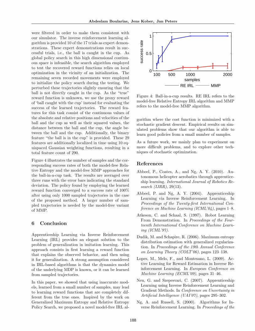
were filtered in order to make them consistent withour simulator. The inverse reinforcement learning al-gorithm is provided 10 of the 17 trials as expert demon-strations. These expert demonstrations result in suc-cessful trials, i.e., the ball is caught in the cup. Asglobal policy search in this high dimensional continu-ous space is infeasible, the search algorithm employedto test the recovered reward functions relies on localoptimization in the vicinity of an initialization. Theremaining seven recorded movements were employedto initialize the policy search during the testing. Weperturbed these trajectories slightly ensuring that theball is not directly caught in the cup. As the “true”reward function is unknown, we use the proxy rewardof ‘ball caught with the cup’ instead for evaluating thesuccess of the learned trajectories. The reward fea-tures for this task consist of the continuous values ofthe absolute and relative positions and velocities of theball and the cup as well as their squared values, thedistance between the ball and the cup, the angle be-tween the ball and the cup. Additionally, the binaryfeature “the ball is in the cup” is provided. These 29features are additionally localized in time using 10 eq-uispaced Gaussian weighting functions, resulting in atotal feature count of 290.

Figure 4 illustrates the number of samples and the cor-responding success rates of both the model-free Rela-tive Entropy and the model-free MMP approaches forthe ball-in-a-cup task. The results are averaged overthree runs with the error bars indicating the standarddeviation. The policy found by employing the learnedreward function converged to a success rate of 100%after using only 1000 sampled trajectories in the caseof the proposed method. A larger number of sam-pled trajectories is needed by the model-free variantof MMP.

6 Conclusion

Apprenticeship Learning via Inverse ReinforcementLearning (IRL) provides an elegant solution to theproblem of generalization in imitation learning. Thisapproach consists in first learning a reward functionthat explains the observed behavior, and then usingit for generalization. A strong assumption consideredin IRL-based algorithms is that the dynamics modelof the underlying MDP is known, or it can be learnedfrom sampled trajectories.

In this paper, we showed that using inaccurate mod-els, learned from a small number of samples, may leadto learning reward functions that are completely dif-ferent from the true ones. Inspired by the work onGeneralized Maximum Entropy and Relative EntropyPolicy Search, we proposed a novel model-free IRL al-

100 500 1000 20000

0.5

1

samples

succ

ess

rate

RE IRL MMP

Figure 4: Ball-in-a-cup results. RE IRL refers to themodel-free Relative Entropy IRL algorithm and MMPrefers to the model-free MMP algorithm.

gorithm where the cost function is minimized with astochastic gradient descent. Empirical results on sim-ulated problems show that our algorithm is able tolearn good policies from a small number of samples.

As a future work, we mainly plan to experiment onmore difficult problems, and to explore other tech-niques of stochastic optimization.

References

Abbeel, P., Coates, A., and Ng, A. Y. (2010). Au-tonomous helicopter aerobatics through apprentice-ship learning. International Journal of Robotics Re-search (IJRR), 29(13).

Abbeel, P. and Ng, A. Y. (2004). ApprenticeshipLearning via Inverse Reinforcement Learning. InProceedings of the Twenty-first International Con-ference on Machine Learning (ICML’04), pages 1–8.

Atkeson, C. and Schaal, S. (1997). Robot LearningFrom Demonstration. In Proceedings of the Four-teenth International Conference on Machine Learn-ing (ICML’97).

Dudik, M. and Schapire, R. (2006). Maximum entropydistribution estimation with generalized regulariza-tion. In Proceedings of the 19th Annual Conferenceon Learning Theory (COLT’06), pages 123–138.

Lopes, M., Melo, F., and Montesano, L. (2009). Ac-tive Learning for Reward Estimation in Inverse Re-inforcement Learning. In European Conference onMachine Learning (ECML’09), pages 31–46.

Neu, G. and Szepesvari, C. (2007). ApprenticeshipLearning using Inverse Reinforcement Learning andGradient Methods. In Conference on Uncertainty inArtificial Intelligence (UAI’07), pages 295–302.

Ng, A. and Russell, S. (2000). Algorithms for In-verse Reinforcement Learning. In Proceedings of the

189


Seventeenth International Conference on MachineLearning (ICML’00), pages 663–670.

Peters, J., Mulling, K., and Altun, Y. (2010). Rela-tive Entropy Policy Search. In Proceedings of theTwenty-Fourth National Conference on Articial In-telligence (AAAI’10).

Pomerleau, D. (1989). ALVINN: An AutonomousLand Vehicle in a Neural Network. In Neural Infor-mation Processing Systems (NIPS’89), pages 769–776.

Ramachandran, D. and Amir, E. (2007). Bayesian In-verse Reinforcement Learning. In Proceedings of Thetwentieth International Joint Conference on Artifi-cial Intelligence (IJCAI’07), pages 2586–2591.

Ratliff, N., Bagnell, J., and Zinkevich, M. (2006).Maximum Margin Planning. In Proceedings of theTwenty-third International Conference on MachineLearning (ICML’06), pages 729–736.

Ratliff, N., Silver, D., and Bagnell, A. (2009). Learn-ing to Search: Functional Gradient Techniques forImitation Learning. Autonomous Robots, 27(1):25–53.

Schaal, S. (1999). Is Imitation Learning the Route toHumanoid Robots? Trends in Cognitive Sciences,3(6):233–242.

Syed, U., Bowling, M., and Schapire, R. E. (2008). Ap-prenticeship Learning using Linear Programming.In Proceedings of the Twenty-fifth InternationalConference on Machine Learning (ICML’08), pages1032–1039.

Syed, U. and Schapire, R. (2008). A Game-TheoreticApproach to Apprenticeship Learning. In Ad-vances in Neural Information Processing Systems 20(NIPS’08), pages 1449–1456.

Ziebart, B., Bagnell, A., and Dey, A. (2010).Modeling Interaction via the Principle of Max-imum Causal Entropy. In Proceedings of theTwenty-seventh International Conference on Ma-chine Learning (ICML’10), pages 1255–1262.

Ziebart, B., Maas, A., Bagnell, A., and Dey, A. (2008).Maximum Entropy Inverse Reinforcement Learn-ing. In Proceedings of The Twenty-third AAAI Con-ference on Artificial Intelligence (AAAI’08), pages1433–1438.

relative entropy inverse reinforcement...

Documents