USGS-OFR-95-555 USGS-OFR-95-555

U.S. DEPARTMENT OF THE INTERIOR

U.S. GEOLOGICAL SURVEY

RELATIVE PERFORMANCE OF SEVERAL INEXPENSIVE ACCELEROMETERS

by

John R. Evans 1 and John A. Rogers 1

Open-File Report 95-555

This report is preliminary and has not been reviewed for conformity with U.S. Geological Survey editorial standards or the North American Stratigraphic Code. Any use of trade, pro­ duct or firm names is for descriptive purposes only and does not imply endorsement by the U.S. Government.

! 345 Middlefield Road, MS-977, Menlo Park, California, 94025.

-2-

Contents

Introduction .............................................................................................................................. 3Sensor Descriptions .................................................................................................................. 3

Kinemetrics FBA-ll .................................................................................................. 4Analog Devices ADXL05-ENG ............................................................................... 4Lucas Schaevitz S05E-005 ....................................................................................... 4CFX USS-1 ............................................................................................................... 5Silicon Microstructures 7170-010 ............................................................................. 5Centurion Instrument 8085EXP ................................................................................ 5Analysis & Technology DRB400 ............................................................................. 5

Test Conditions ........................................................................................................................ 6Sensitivity Test ......................................................................................................................... 7Sensor Noise ............................................................................................................................. 9Relative Transfer Functions .....................................................................................................11Cross-axis Sensitivity ...............................................................................................................12Summary ...................................................................................................................................13Acknowledgements ..................................................................................................................15References ................................................................................................................................15

FiguresCaptions ....................................................................................................................................16Figures (sequentially by Figure number) ................................................................................18

TablesTable la: Sensor Offset at ADC Output (test group 1) ........................................................ 8Table \b: Sensor Offset at ADC Output (test group 2) ........................................................ 8Table Ic: Sensor Sensitivity at ADC Output ........................................................................ 9Table 2: System RMS Noise in Two Bands .........................................................................10Table 3: Summary of Results .................................................................................................14

-3-

IntroductionWe examined the performance of several low-cost accelerometers for highly cost-driven

applications in recording earthquake strong motion. We anticipate applications for such sen­ sors in providing the lifeline and emergency-response communities with an immediate, comprehensive picture of the extent and characteristics of likely damage. We also foresee their use as "filler" instruments sited between research-grade instruments to provide spatially detailed and near-field records of large earthquakes (on the order of 1000 stations at 600-m intervals in San Fernando Valley, population 1.2 million, for example). The latter applications would provide greatly improved attenuation relationships for building codes and design, the first examples of mainshock information (that is, potentially nonlinear regime) for microzona- tion, and a suite of records for structural engineers. We also foresee possible applications in monitoring structural inter-story drift during earthquakes, possibly leading to local and remote alarm functions as well as design criteria.

This effort appears to be the first of its type at the USGS. It is spurred by rapid advances in sensor technology and the recognition of potential non-classical applications. In this report, we estimate sensor noise spectra, relative transfer functions and cross-axis sensi­ tivity of six inexpensive sensors. We tested three micromachined ("silicon-chip") sensors in addition to classical force-balance and piezoelectric examples. This sample of devices is meant to be representative, not comprehensive.

Sensor noise spectra were estimated by recording system output with the sensor mounted on a pneumatically supported 545-kg optical-bench isolation table. This isolation table appears to limit ground motion to below our system noise level. These noise estimates include noise introduced by signal-conditioning circuitry, the analog-to-digital converter (ADC), and noise induced in connecting wiring by ambient electromagnetic fields in our suburban laboratory. These latter sources are believed to dominate sensor noise in the quieter sensors we tested. Transfer functions were obtained relative to a research grade force-balance accelerometer (a Kinemetrics FBA-11) by shaking the sensors simultaneously on the same shake table and taking spectral ratios with the output of the FBA-11. This reference sensor is said to have 120 db dynamic range (~±20 bits, though we only digitized it at 16 bits resolu­ tion and drove it with relatively small signals). We did not test temperature sensitivity, which is thought to be a significant issue at least for the silicon devices.

Though these tests were not designed to be definitive (our anticipated applications do not demand research-grade precision), our tests do appear to have been successful in estimating relative transfer functions from about 0.3 to 50 Hz. Most sensors performed adequately in this range, with essentially flat relative transfer functions. Noise tests appear to measure sen­ sor noise well for the noisier (generally less expensive) instruments from about 0.1 to 50 Hz.

In this report, we use the units g = 980.665 cm/s2 and mg = 0.001 g = 0.980665 cm/s2. The "gal" not used here, though common in geophysics is defined as 1 cm/s2. We occa­

sionally use the |0.g = 10~6 g. "RMS" means root mean square, ( 2 an ) 1/2 -

Sensor DescriptionsWe seek sensors which (1) are very inexpensive, (2) are robust to mechanical abuse, (3)

will operate reliably after a passage of years without routine maintenance, (4) respond linearly

-4-

to at least ±3 g acceleration, (5) have noise below about 0.003 g RMS over the band of interest (but ideally < 0.001 g peak-to-peak, equivalent to 12-bits resolution over ±1 g and below the nominal 0.001-g threshold of human perception (Richter, 1958)), (6) have essen­ tially flat transfer functions from <0.5 Hz to >10.0 Hz (preferably from <0.1 Hz to >35 Hz), (7) are able to operate with their active axis in any orientation; and (8) are able to operate over a temperature range of about -10 °C to +50 °C. Some long-term (longer than minutes) temperature drift is acceptable (we anticipate using some thermal insulation around the sensor and placement of the sensor in a shallow vault or a building). The 0.003 g RMS noise floor (or about 9-bits resolution between ±1 g) will be discussed further in the section on sensor noise.

Our original aim was to characterize only inexpensive micromachined accelerometers, since we believed these to be the most promising option. However, it became apparent that other technologies may be applicable to our problem, so we included examples of them. A significant percentage of the sensors tested here were one-off test units or engineering samples provided for our tests. Others were commercially available devices, however, it is clear that this is a rapidly evolving industry. The specifications and prices given here are from manufacturers' information, some by voice. Though we believe this information to be current as of March, 1995, we make no claim of accuracy or currency, and give the following descriptions solely for context, subject to the disclaimer on the title page of this report.

All but three sensors (8085EXP, DRB400, and 7170-010) have adequately high-level outputs for direct input to the ADC. Measured sensitivities (including our buffer gain for those three sensors) are given in Tables la-c

Kinemetrics FBA-11:

Our reference instrument, the Kinemetrics FBA-11 (serial number 35754), is a type widely used in structural-engineering and seismological research. It is a capacitive-sense electromagnetic-feedback force-balance accelerometer (FBA). Its maker specifies a signal-to- noise ratio of 120 db from DC to its resonant frequency of 50 Hz (hence, 2 |ig worst case resolution). For comparison in the context of our current goals, we compare unit costs in moderately large quantity purchases, nominally quantity 100+. In similar quantity (85+) the FBA-11 costs $760.

Analog Devices ADXL05-ENG:

This device is a pre-release engineering sample ("-ENG") of the ADXL05 micromachined FBA. It has internal signal conditioning and temperature compensation, as well as an uncommitted operational amplifier on the same die. Manufacturer's specifications indicate that it becomes non-linear at about +5 g. The ADXL05 is designed to survive 500 g shock (0.5 ms) while operating. (Production devices were scheduled to be available in May, 1995, with "incremental" improvements in noise and DC drift over the "-ENG" part tested here.) The ADXL05 uses a capacitive-sense electrostatic-feedback arrangement with a (polysilicon) proof mass of about 0.2 micrograms. It is mounted in a TO-100 container (a squat metal can 8.51 mm in diameter). Its cost has been announced as $15 each (100 quan­ tity) for the 0 to +70 °C "JH" version.

Lucas Schaevitz S05E-005:Lucas Control Systems supplied a Lucas Schaevitz device. It is a higher grade

(less noisy) silicon micromachined accelerometer with signal conditioning, employing

- 5 -

temperature-compensated piezoresistive sense. It is an open loop accelerometer (not an FBA) packaged in a NEMA-4 housing (plastic rectangular solid 20.57x39.61x36.06 mm high, plus a small base plate). It is designed to withstand 400 g static, 1000 g shock (1 ms), and 20 g RMS vibration. The resonant frequency is above 400 Hz. Manufacturer's specifications indi­ cate that it becomes non-linear at ±5 g. The S05E-005's cost is $259 (100 quantity).

CFX USS-1:

The USS-1 is a miniature FBA derived from aircraft sensors, but held down in price by various design, test, and manufacturing measures. The USS-1 is packaged in a small plastic cylinder with flat bottom (-g end) and rounded top (28 mm diameterx29 mm height); it is epoxy potted and can be mounted with epoxy also. The usual clipping range is ±2 g, with DC-to-25 Hz frequency response. The USS-1 is designed for a temperature range of -20 to +75 °C and will withstand a 500 g shock (1 ms) or 10 g RMS vibration from 20 to 2000 Hz. The cost is $98.95 in 100 quantity.

Silicon Microstructures Inc. 7170-010:

The 7170-010 is a capacitive-sense open-loop silicon micromachined accelerometer with ±10 g range. (A ±2 g version also is available; we have been told that intermediate ranges could be custom built if a large order were guaranteed these might have better resolution than the -010.) The 7170-010 has a resonant frequency of 3.3 kHz, and lower output range than the other signal-conditioned units (to accommodate the larger clipping range). Since we are using fairly small test signals, we buffered its output through an "OP20" operational amplifier at lOx gain with a one-pole low-pass filter at about 60 Hz, bringing its sensitivity into the same range as most other sensors and providing some anti-alias protection. The sen­ sor and signal-conditioning circuitry are packaged in a plastic carrier 27.1x20.6x8.2 mm high, with perforated side tabs for bolting it down. Its cost is $120 in quantity 100.

Centurion Instrument Corp. "8085EXP":

This is an experimental device provided for these tests. It is a modified version of Centurion's 8085 accelerometer, so we designate it the "8085EXP". It uses a synthetic "PZT" piezoelectric crystal in an open-loop configuration, with limited temperature compensa­ tion and an internal unity-gain impedance-matching circuit. It clips far outside our range of interest, so effective clipping is determined by external signal-conditioning circuitry. The price is undetermined but could run as low as $100 in large quantity for a triaxial device (unless otherwise stated, the prices quoted in this report are for monoaxial devices). Current housing is a small stainless-steel cylinder the manufacturer uses for such test devices. Because of its low sensitivity, we buffered its output through an "OP20" operational amplifier at 30x gain with a one-pole low-pass filter at about 60 Hz, bringing its sensitivity into the same range as most other sensors and providing some anti-alias protection.

Analysis & Technology, Inc DRB400:

This is an experimental piezoelectric accelerometer using a polymer film as the sense element (AMP 28 monoaxial PVDF). As described by J. Kassal (written communication, 1995), it operates through a proprietary mechanism to exploit the "3-1" mode (i.e., force applied parallel to the axis along which the polymer sheet was originally stretched during manufacture). Robustness is only coarsely tested, but probably reaches 100 g. Vibration at 20 g probably would cause failure "after several hours". The mechanism resonates at about 60 Hz, which could be raised at the expense of greater sensor noise. It probably clips near ±3

-6-

g. Cost, without signal conditioning, would be about $30 in quantity 1000, but is not well established. Signal conditioning might add $10 more. Preliminary signal-conditioning hardware supplied by the manufacturer imposes a band pass anticipated from about 0.1 to 25 Hz. The lowest frequency achievable depends critically on amplifier input impedance, which must be very high. Our tests refer to the output of the signal-conditioning hardware and prob­ ably do not reflect ultimate performance limits of the sensor. We buffer the output of the signal-conditioning hardware through an "OP20" operational amplifier, at lOx gain with a one-pole low-pass filter at about 60 Hz to bring its output more in line with the other sensors.

Analysis & Technology also provided a more sensitive device (UB5000) which would have a bandpass of about 0.3 to 30 Hz with this amplifier. It would be about twice as expen­ sive. Due to limited testing time, we only tested the DRB400, which exhibits a more useful bandpass and lower price.

Test ConditionsSensor tests were performed in two groups, each with three sensors under test along with

the reference FBA-11. (Grouping was determined simply by equipment availability and does not imply any qualitative association between sensors within a group.) Resulting signals were recorded simultaneously on a PC-compatible computer, using a 16-bit ADC (gain 1, 200 samples/s) and program XRTP (Lee, 1994). There was little or no shielding of leads, except for the two sensors with especially low-level outputs (the DRB400 has coax connections, the 8085EXP a twisted pair). Most analysis and graphics were done with UNIX version 4.0 of PITSA (Scherbaum and Johnson, 1993) and a newer, pre-release version of PITSA.

Tests were made at room temperature in the basement of a building in Menlo Park, Cali­ fornia, about 3 m below grade on a concrete floor slab in alluvium. This is a metropolitan region of suburbs and light industry, with a major freeway 2 km away, a major surface street adjacent, and a busy rail line about 1 km away. The largest seismic-noise source probably is the building machinery.

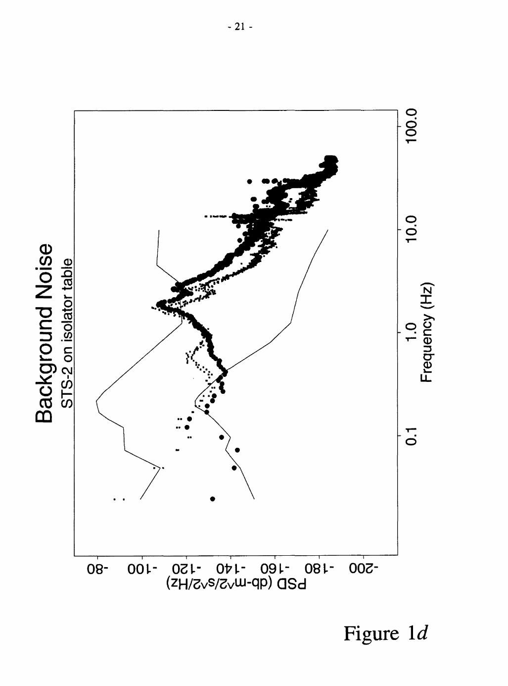
Noise tests were performed in a room chosen for its maximal distance from these and other noise sources, with the sensors mounted on a pneumatically isolated massive platform designed for optical-bench work (545-kg Granitru table supported by Newport Type XL-A pneumatic isolators). Estimated transfer functions of this table are shown in Figure \a,b, the ratios being between ambient-noise samples recorded four hours apart on the table and on the floor next to the table.

Though the samples are not simultaneous, two significant peaks near 1 Hz are evident; these are similar to the manufacturers' estimate of the table's resonant frequency. These peaks cause significant (~10x) amplification of like-frequency ground noise. Above that fre­ quency ground noise is attenuated, but below it long-period tilt of the table upon its pneu­ matic legs creates large signals on horizontal components of the Streckeisen STS-2 seismometer we used (the STS-2 is an ultra-long-period FBA producing output proportional to ground velocity). The absolute spectra of the noise samples are compared to the USGS noise models of Peterson (1993) in Figures \c,d. Above its resonance frequencies, the isolator table is a tolerably quiet, though not ideal site for measuring sensor noise (Figure Id). At and below the resonant frequency, it is more appropriate to mount sensors directly to the floor slab. Long-period noise (>0.3 s) probably is exaggerated in our noise tests.

-7-

In each test group, the FBA-11 and three inexpensive sensors were bolted to a common aluminum plate (6.35 mm thick and roughly 20 cm on a side), and aligned to one another and to the test equipment by careful use of a bubble level and a drafting triangle with visual sight­ ing along machined or molded edges. The most difficult sensor to align was the ADXL05- ENG, which is supplied in a TO-100 container with a small alignment tab on one edge in the direction of the device's positive-acceleration axis (late cross-axis tests suggest this sensor may have been -5° out of alignment during most of our tests). The other sensors were aligned within ±0.5°, not including any internal misalignments. (One might anticipate rela­ tively large internal misalignments on the two experimental units (DRB400, 8085EXP), which is suggested by the cross-axis tests.)

Sensitivity TestWe calibrated the entire system end-to-end (from sensor through signal conditioning and

ADC) with a simple tilt test on a machine-tool tilt table (Enco 200-1063) with the accelerometers rigidly clamped to the tilt table. Measurements were made in only one direc­ tion of tilt change, to obviate hysteresis in the tilt table. The table's tilt can be read to five arc-seconds on a vernier dial. Results are given in Figures 2a-c and Tables la-c.

We took readings at seven angles from about -30° to about +30° (i.e., ±0.5 g). Zero tilt was set in both axes within about 0.5° with a bubble level. (For comparison, Figures 2b and c show the anticipated effect of a 0.5° misalignment in the direction of the +g axes of the accelerometers.) Alignment of the accelerometers with the tilt vector was accomplished with a drafting triangle and careful visual sighting along the relevant edge of the tilt table. Align­ ment accuracy is about ±0.5°, excepting the caveats given above. The DC offset reading was supplied by the PC, and equals the average ADC output, in digital counts, across the 2.56-s display window. We observed this offset over a period of about 10 s to estimate its stability ("±" in the tables).

We computed sensitivity from the slope of a robustly regressed line (LI norm) in g- versus-counts space (Figures 2a-c). Results are given in Tables la-c and are used to scale ADC output in all subsequent tests. The piezoelectric sensors (DRB400 and 8085EXP) are AC coupled, so their sensitivities could not be determined in this manner. We estimated their sensitivity by setting their transfer functions in Figure Ib to 1.0 at 10 Hz.

-8-

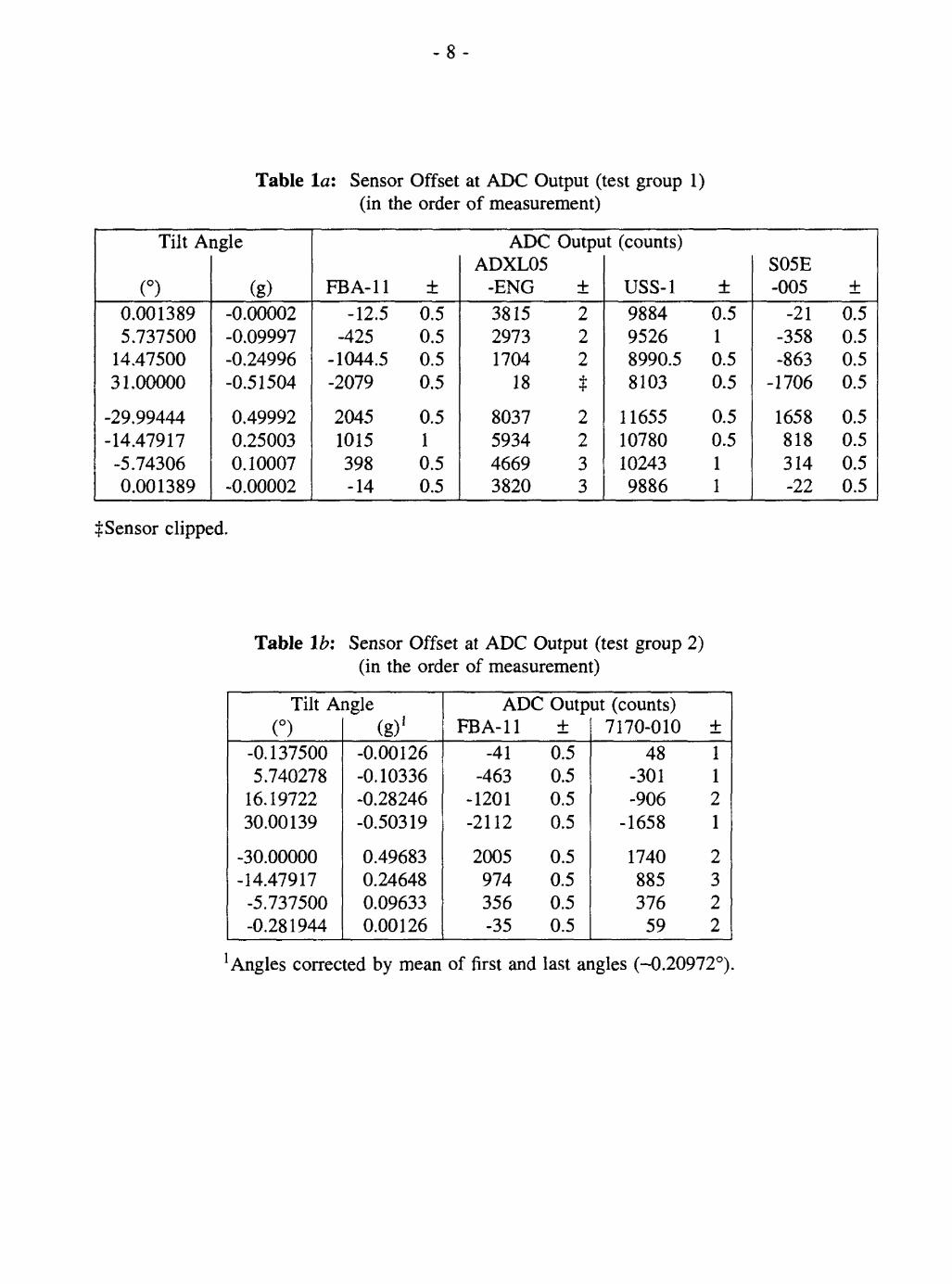
Table la: Sensor Offset at ADC Output (test group 1) (in the order of measurement)

Tilt A

(°)

0.0013895.737500

14.4750031.00000

-29.99444-14.47917-5.743060.001389

tigle

(g)-0.00002-0.09997-0.24996-0.51504

0.499920.250030.10007

-0.00002

FBA-11 ±-12.5 0.5

-425 0.5-1044.5 0.5-2079 0.5

2045 0.51015 1398 0.5-14 0.5

ADC Outpu ADXL05

-ENG ±3815 22973 21704 2

18 t

8037 25934 24669 33820 3

it (counts)

USS-1 ±9884 0.59526 18990.5 0.58103 0.5

11655 0.510780 0.510243 19886 1

S05E -005 ±

-21 0.5-358 0.5-863 0.5

-1706 0.5

1658 0.5818 0.5314 0.5-22 0.5

$ Sensor clipped.

Table Ib: Sensor Offset at ADC Output (test group 2) (in the order of measurement)

Tilt A (°)

-0.1375005.740278

16.1972230.00139

-30.00000-14.47917

-5.737500-0.281944

tigle (g) 1

-0.00126-0.10336-0.28246-0.50319

0.496830.246480.096330.00126

ADC Outp FBA-11 ±

-41 0.5-463 0.5

-1201 0.5-2112 0.5

2005 0.5974 0.5356 0.5-35 0.5

ut (counts) 7170-010 ±

48 1-301 1-906 2

-1658 1

1740 2885 3376 2

59 2

'Angles corrected by mean of first and last angles (-0.20972°).

-9-

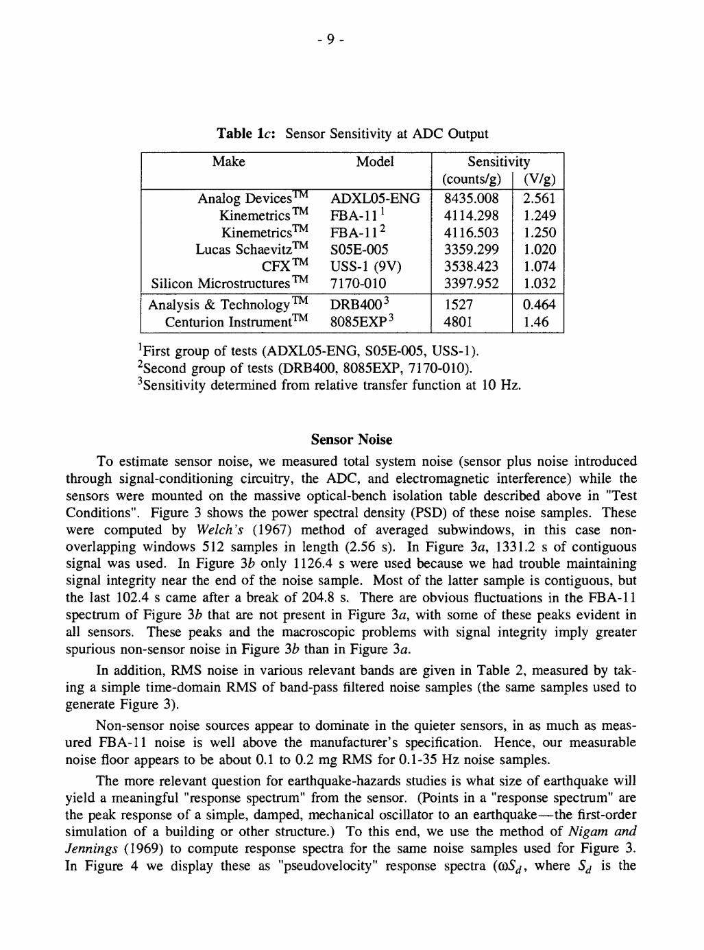
Table Ic: Sensor Sensitivity at ADC Output

Make

Analog Devices Kinemetrics Kinemetrics

Lucas Schaevitz CFX

Silicon Microstructures

Analysis & Technology Centurion Instrument

Model

ADXL05-ENG FBA-11 1 FBA-11 2

S05E-005 USS-1 (9V) 7170-010DRB400 3

8085EXP 3

Sensiti\ (counts/g)8435.008 4114.298 4116.503 3359.299 3538.423 3397.952

1527 4801

ity (V/g)2.561 1.249 1.250 1.020 1.074 1.0320.464 1.46

! First group of tests (ADXL05-ENG, S05E-005, USS-1). 2Second group of tests (DRB400, 8085EXP, 7170-010). 3 Sensitivity determined from relative transfer function at 10 Hz.

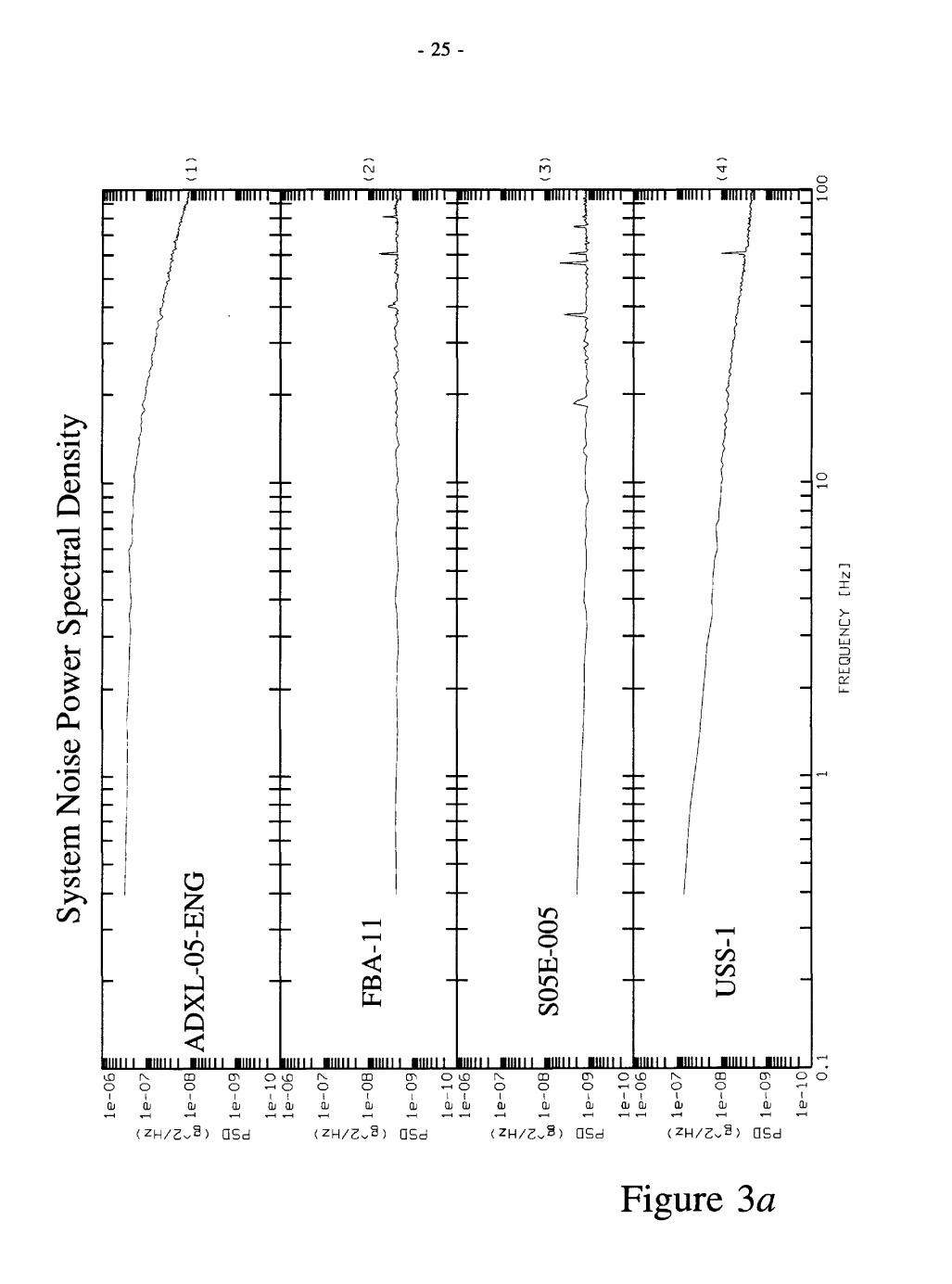
Sensor NoiseTo estimate sensor noise, we measured total system noise (sensor plus noise introduced

through signal-conditioning circuitry, the ADC, and electromagnetic interference) while the sensors were mounted on the massive optical-bench isolation table described above in "Test Conditions". Figure 3 shows the power spectral density (PSD) of these noise samples. These were computed by Welch's (1967) method of averaged subwindows, in this case non- overlapping windows 512 samples in length (2.56 s). In Figure 3a, 1331.2 s of contiguous signal was used. In Figure 3b only 1126.4 s were used because we had trouble maintaining signal integrity near the end of the noise sample. Most of the latter sample is contiguous, but the last 102.4 s came after a break of 204.8 s. There are obvious fluctuations in the FBA-11 spectrum of Figure 3b that are not present in Figure 3a, with some of these peaks evident in all sensors. These peaks and the macroscopic problems with signal integrity imply greater spurious non-sensor noise in Figure 3b than in Figure 3a.

In addition, RMS noise in various relevant bands are given in Table 2, measured by tak­ ing a simple time-domain RMS of band-pass filtered noise samples (the same samples used to generate Figure 3).

Non-sensor noise sources appear to dominate in the quieter sensors, in as much as meas­ ured FBA-11 noise is well above the manufacturer's specification. Hence, our measurable noise floor appears to be about 0.1 to 0.2 mg RMS for 0.1-35 Hz noise samples.

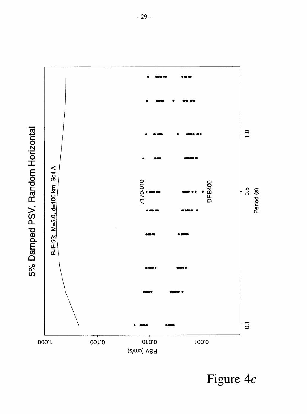
The more relevant question for earthquake-hazards studies is what size of earthquake will yield a meaningful "response spectrum" from the sensor. (Points in a "response spectrum" are the peak response of a simple, damped, mechanical oscillator to an earthquake the first-order simulation of a building or other structure.) To this end, we use the method of Nigam and Jennings (1969) to compute response spectra for the same noise samples used for Figure 3. In Figure 4 we display these as "pseudovelocity" response spectra (coS^, where Sd is the

- 10-

displacement response spectrum of Nigam and Jennings and CO is the natural (angular) fre­ quency of the "structure" responding to the earthquake). For Figure 4 we chose 5% damped response spectra, the standard commonly used for structural engineering. We scatter-plot response spectra for all the valid samples from each sensor (13 for group one: ADXL05- ENG, FBA-11, S05E-005, USS-1; 11 for group two: DRB400, 8085EXP, FBA-11, 7170- 010). For comparison, the smooth line in each frame of Figure 4 is the estimated response spectrum of the smallest earthquake shaking that can be estimated validly with the models of Boore et al. (1993) the most distant event of the smallest magnitude, recorded on bedrock ("soil A"). It is clear that all the sensors we tested are adequate for computing pseudovelocity response spectra with better than an order of magnitude in signal-to-noise ratio for the weak­ est shaking predicted by Boore et al. (1993).

Our requirement for a noise floor of 3 mg RMS, rather than a lower value, deserves additional comment. The pseudoacceleration (co25^) expected from the hypothetical earth­ quake in Figure 4 is as low as 1.3 mg at 2-s period, so one might anticipate requiring a 1 mg or lower noise floor. However, the applications for these sensors are likely to be related prin­ cipally to structural hazards in urban areas, hence the pseudovelocity response spectrum is the relevant data space. In that space, even the noisiest sensor (Figure 4d) is an order of magni­ tude quieter than shaking from a moderate, distal earthquake. Given that near-field records of moderate or larger earthquakes from sensors in urban areas (typically soil types B and C) are of greatest utility, we consider the 3 mg RMS noise floor adequate. Lower noise floors yield additional applications for the records, but must be evaluated in the context of the anticipated cost-driven environment.

Table 2: System RMS Noise in Two Bands t

Make Model

Analog Devices ADXL05-ENG Kinemetrics FBA-11

Lucas Schaevitz S05E-005 CFX USS-1 (9V)

Analysis & Technology DRB400 Centurion Instrument 8085EXP

Kinemetrics FBA-11 Silicon Microstructures 7170-010

BJF-93, smallest valid event $ Richter's (1958) Felt Threshold

System noise (R 0.1-35.0 Hz

2.210 0.2821 0.2062 0.63380.5071 0.7915 0.3194 1.595

MS, mg) for: 0.5-10.0 Hz

1.450 0.1448 0.1066 0.41280.2235 0.4238 0.1604 1.011

12.9 1

tTime-domain computation of RMS from noise samples filtered with corners as indicated. Slope in transition band is 120 db/octave (a PITS A Butterworth bandpass filter of three sec­ tions run both forward and backward across the data). Tests were performed in two groups, with the FBA-11 included in each group. The first group included the ADXL05-ENG, S05E- 005, and USS-1 (two micromachined and one miniature FBA). The second group included the DRB400, 8085EXP, and 7170-010 (two piezoelectric and one micromachined).\Eoore et al. (1993) maximum site acceleration for an earthquake of magnitude 5.0 at a dis­ tance of 100 km on their soil type "A" (shear-wave velocity over 750 m/s). This is the light­ est shaking validly modeled by Boore et al.

-11 -

Relative Transfer FunctionsThis test was simply to determine if sensor performance is adequate (ideally, flat within a

few percent) within the band we desire to use. At a minimum, we need useful response between 10 and 0.5 Hz, corresponding to nominal resonant frequencies of buildings one to 20 stories high. Wider band limits (0.1 to 35 Hz) are desirable for taller buildings and for certain research uses that may be attempted.

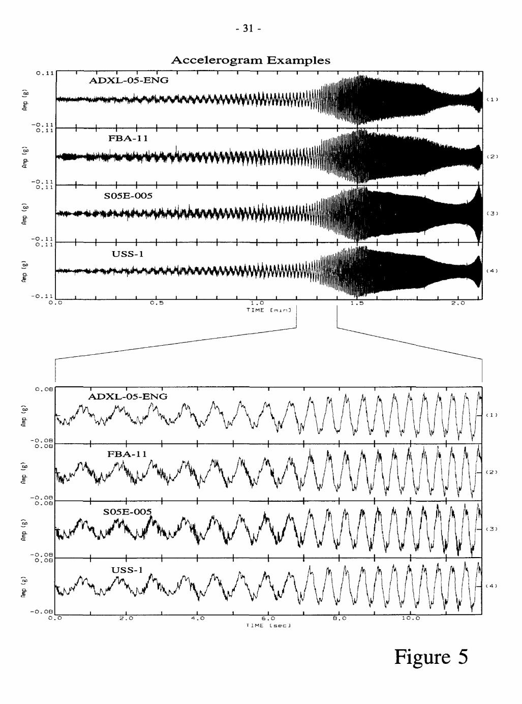
We mounted sensor sets on a modest shake table and drove the shake table with the sinusoid from a synthesizing function generator (a Wavetek model 23). This function gen­ erator has a continuous rotary input dial to adjust its parameters, including the frequency of the sine wave. We drove this dial by hand to approximate a logarithmically swept sine chirp lasting from 60.0 to 163.7 s. Duration variability is due to human factors; this variability may be helpful in reducing systematics in the final ensemble averages and in any case has no nega­ tive consequences. We did equal numbers (nine each) of upward and downward sweeps between 0.1 and 50 Hz. A typical upward sweep is shown in Figure 5.

It is clear that the shake table responds with different amplitude across the driven bandwidth. In particular, the tables response is poor at longer periods, with significant high- frequency noise introduced by the unevenness of aging support bearings in the table.

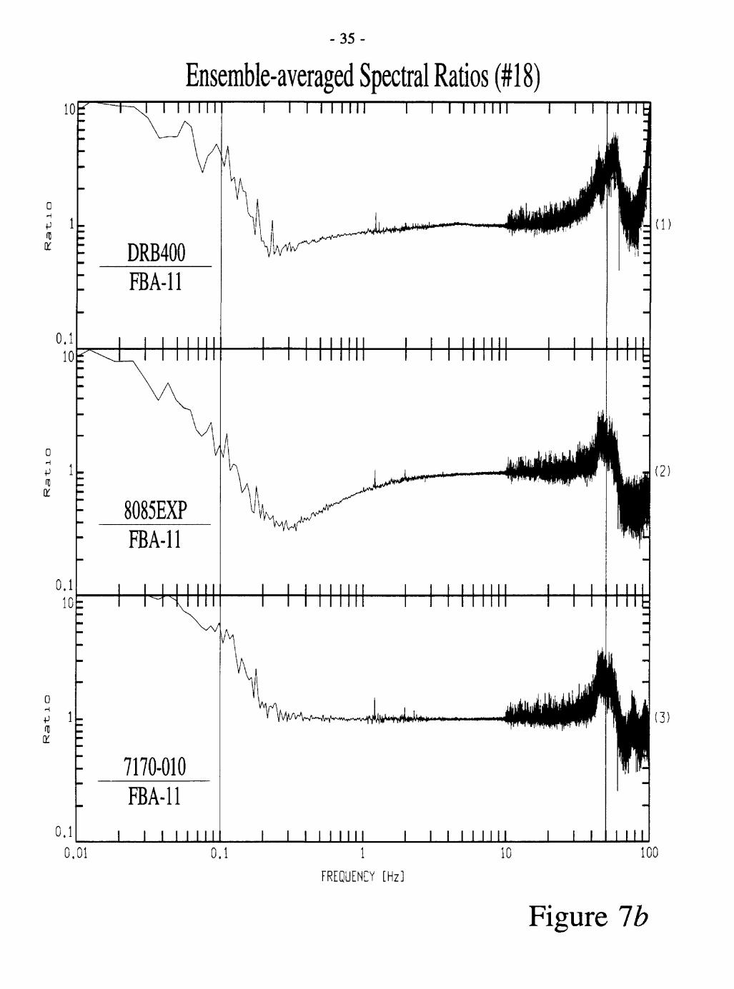
Spectra of each sweep (with a 5% cosine taper on each end and padded to 32,768 points with zeros) were taken. Spectra for the sweep shown in Figure 5 are shown in Figures 6a,b. Ratios of the test-sensor spectra to the FBA-11 spectrum were formed for each sweep. (The values of these spectral ratios are dubious near the 50 Hz resonant frequency of the FBA-11.) Lastly, the 18 available spectral ratios for each test sensor were ensemble averaged to produce the relative transfer functions shown in Figure la, b. The side-bar at the end of this section indicates what these ratios approximate a transfer function if FBA-11 response is flat.

The three micromachined sensors (ADXL05-ENG, S05E-005, and 7170-010) and the miniature FBA (USS-1) all have flat response spectra across the minimum desirable band and beyond. The inefficiency of the shake table at long periods make our spectral ratios uncertain below about a few tenths of one Hertz, though they appear plausible to as low as 0.1 Hz in comparisons between Figures 6a and 3. Transfer functions for the piezoelectric sensors, par­ ticularly the 8085EXP but also the DRB400, are less adequate. These may still be useful if more closely tailored to the function and corrected during processing. Of course, such correc­ tions complicates usage and calibration.

The test-sensor spectra in Figure 7 are actuallyS T + S X TX

C ^^ __ " " f -t \ 111 J 17 T1 i 17 T1 ^

plus noise, where r(to) is the axial excitation of the shake table, rx(co) is the cross-axis exci­ tation of the table, 5(co) and 5 x(to) are the axial and cross-axial transfer functions of the test sensor, and F(co) and F x(tO) similarly of the reference FBA-11. Since F xrx and S X TX are the products of small values

r ~AZ_ A m CS ~FT~F- (2)

- 12-

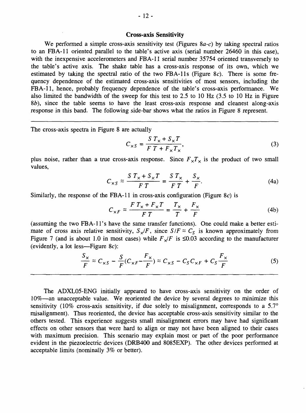
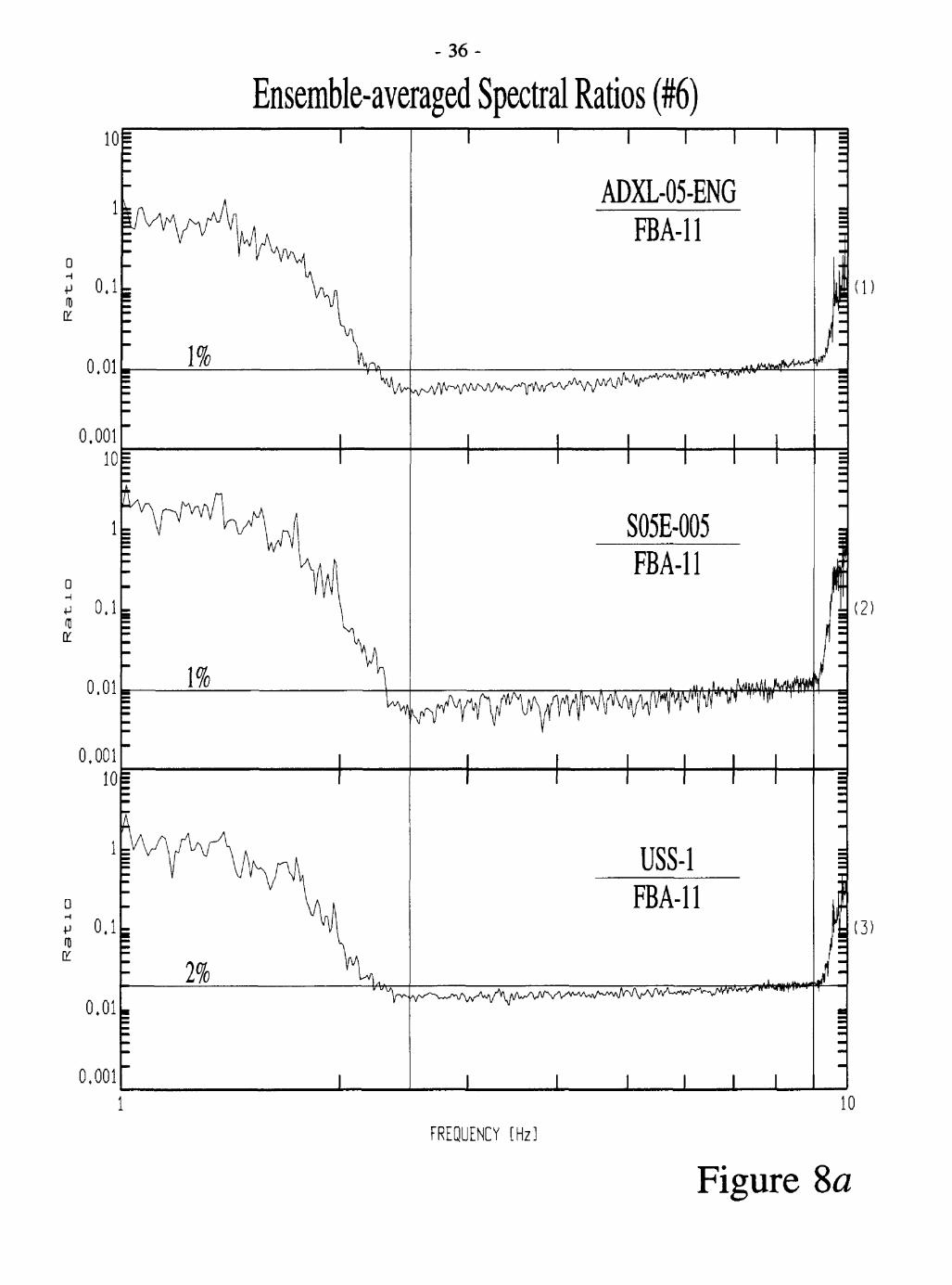
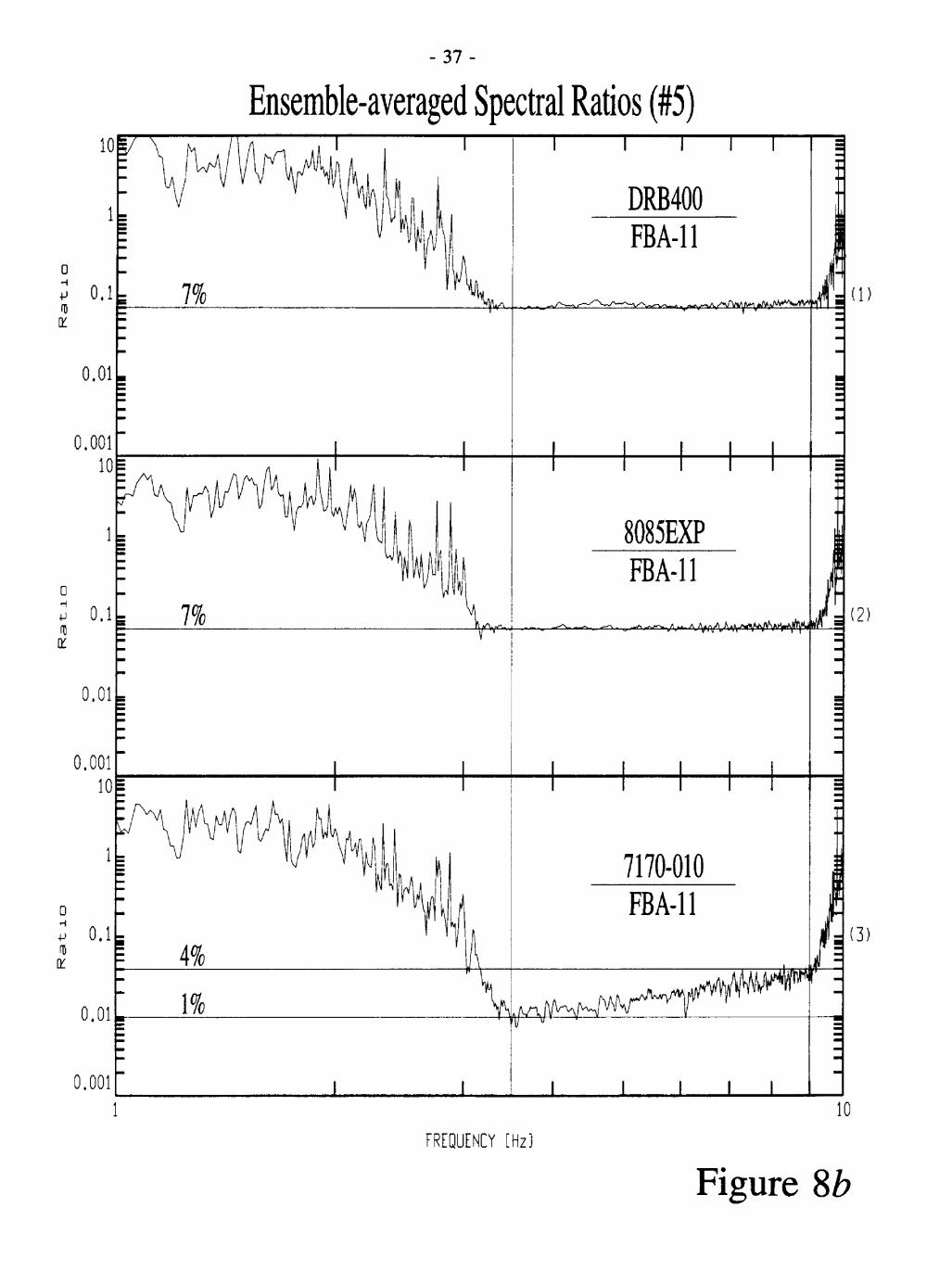
Cross-axis SensitivityWe performed a simple cross-axis sensitivity test (Figures 8a-c) by taking spectral ratios

to an FBA-11 oriented parallel to the table's active axis (serial number 26460 in this case), with the inexpensive accelerometers and FBA-11 serial number 35754 oriented transversely to the table's active axis. The shake table has a cross-axis response of its own, which we estimated by taking the spectral ratio of the two FBA-lls (Figure 8c). There is some fre­ quency dependence of the estimated cross-axis sensitivities of most sensors, including the FBA-11, hence, probably frequency dependence of the table's cross-axis performance. We also limited the bandwidth of the sweep for this test to 2.5 to 10 Hz (3.5 to 10 Hz in Figure 8Z>), since the table seems to have the least cross-axis response and cleanest along-axis response in this band. The following side-bar shows what the ratios in Figure 8 represent.

The cross-axis spectra in Figure 8 are actually

5 Tx + S X T

plus noise, rather than a true cross-axis response. Since FXTX is the product of two small values,

iJ L y "T" iJy/ O/y ^ X

Similarly, the response of the FBA-11 in cross-axis configuration (Figure 8c) is

F Tx + Fx T Tx FxCx zr = - = + (4b)

x/< WT T F

(assuming the two FBA-11 's have the same transfer functions). One could make a better esti­ mate of cross axis relative sensitivity, S X/F, since SIF~ Cs is known approximately from Figure 7 (and is about 1.0 in most cases) while FX/F is <0.03 according to the manufacturer (evidently, a lot less Figure 8c):

S x 5 Fx Fx~Tr ~ Cxs ~ ~;(CxF T") ~ CxS - Cs CxF + Cs - (5)

The ADXL05-ENG initially appeared to have cross-axis sensitivity on the order of 10% an unacceptable value. We reoriented the device by several degrees to minimize this sensitivity (10% cross-axis sensitivity, if due solely to misalignment, corresponds to a 5.7° misalignment). Thus reoriented, the device has acceptable cross-axis sensitivity similar to the others tested. This experience suggests small misalignment errors may have had significant effects on other sensors that were hard to align or may not have been aligned to their cases with maximum precision. This scenario may explain most or part of the poor performance evident in the piezoelectric devices (DRB400 and 8085EXP). The other devices performed at acceptable limits (nominally 3% or better).

- 13-

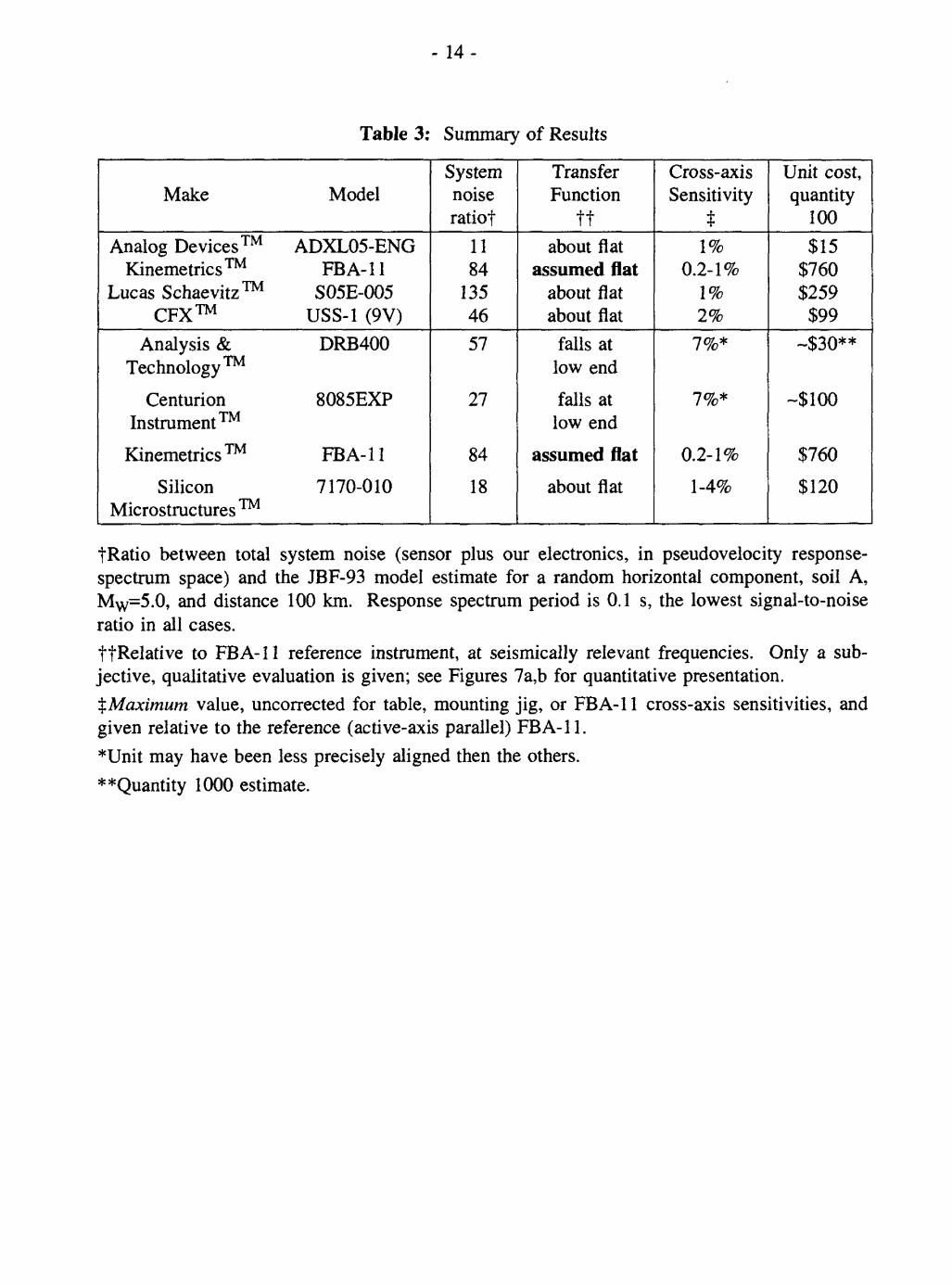
SummaryTable 3 summarizes our results, partly in a subjective manner. For the purposes

described in the Introduction, it appears that (1) the piezoelectric units would introduce undesirable complications because of the low-frequency roll off in their relative transfer func­ tions (and possibly high cross-axis sensitivities); (2) the micromacnined devices and USS-1 miniature FBA all have adequate response functions and cross-axis sensitivity; and (3) all units tested have adequate noise floors. (This noise floor is just barely adequate for the ADXL05-ENG, falling well above the best-ever digitizing quality of SMA-1 optically record­ ing accelerographs (about ±0.26 mg RMS) and near the /ower-quality digitizing now available for those records (about ±2.6 mg RMS) (A. G. Brady, written communication, 1995).) In other words, inexpensive accelerometers have progressed to the point where they have earth­ quake applications, but the noise/cost ratio and noise floor are issues. It is very likely that sensors now available or available within a year will better the SMA-1 best-case noise floor while reaching the $10-$20/component cost range in large quantity.

The SMA-1 is old but is still the most widely deployed strong-motion instrument (about 6000 units). It is the basis of most data now used to create the JBF-93 model (Boore et al., 1993) and similar engineering models. It is quite adequate for damaging levels of ground shaking, if not for subtle modeling of small or distant earthquakes. It is clear that this grade of record has continuing utility (D. Boore and Wm. Joyner, personal communications, 1995) and that digital systems with greatly reduced maintenance requirements and vastly simpler data-collection and data-processing schemes can now be produced for far less cost than the original SMA-1. Hence, the opportunity is at hand for practical "filler" instruments, smarter gas shut-off valves, and many other earthquake mitigation and research uses.

- 14-

Table 3: Summary of Results

Make Model

Analog Devices ADXL05-ENGKinemetrics FBA-11

Lucas Schaevitz S05E-005CFX USS-1 (9V)

Analysis & DRB400Technology

Centurion 8085EXPInstrument

Kinemetrics FB A- 1 1

Silicon 7170-010Microstructures

Systemnoiseratiof

1184

1354657

27

84

18

TransferFunction

ttabout flat

assumed flatabout flatabout flat

falls atlow end

falls atlow end

assumed flat

about flat

Cross-axisSensitivity

$1%

0.2-1%1%2%

7%*

7%*

0.2-1%1-4%

Unit cost,quantity

100$15

$760$259

$99~$30**

~$100

$760

$120

tRatio between total system noise (sensor plus our electronics, in pseudovelocity response- spectrum space) and the JBF-93 model estimate for a random horizontal component, soil A, Mw=5.0, and distance 100 km. Response spectrum period is 0.1 s, the lowest signal-to-noise ratio in all cases.tfRelative to FBA-11 reference instrument, at seismically relevant frequencies. Only a sub­ jective, qualitative evaluation is given; see Figures 7a,b for quantitative presentation.^Maximum value, uncorrected for table, mounting jig, or FBA-11 cross-axis sensitivities, and given relative to the reference (active-axis parallel) FBA-11.*Unit may have been less precisely aligned then the others.**Quantity 1000 estimate.

- 15-

AcknowledgementsWe wish to thank the manufacturers and their representatives for the generous loan of

each sensor tested, some for periods of many months while we organized this effort. The manufacturers are listed in Tables Ic, 2, and 3; additional manufacturers' representatives assisted in arranging these loans, in particular Electronic Engineering Associates (for Lucas ), and Dugan Technologies (for Silicon Microstructures ). We are also indebted to Quanterra for their loan of the 24-bit digitizer used to evaluate isolation-table noise con­ ditions and for consultations about its calibration. We also thank Joe Fletcher for his review of this manuscript. Willie Lee assisted greatly in making the PC software work correctly in our application, and is largely responsible for the isolator-table transfer-function data gather­ ing. Steve Hickman graciously loaned us the use of this isolation-table and laboratory space. Mitch Robinson made a valiant effort to provide a format-translation code. Certainly not least, Frank Scherbaum and Joachim Wassermann gave extensive aid in the use of PITSA, with which nearly all this work was performed. Joachim implemented the PSD estimator in PITSA and made it available to us prior to general release. Both responded to numerous queries well beyond the call of duty.

ReferencesBoore, D. M., W. B. Joyner, and T. E. Fumal, Estimation of response spectra and peak

accelerations from western North American earthquakes: an interim report, U.S. Geol. Surv. Open File Rep., 93-509, 72 pp., 1993.

Lee, W. H. K., Toolbox for Seismic Data Acquisition, Processing, and Analysis, IASPEI Software Library, Second Edition, Volume I, Internal. Assoc. Seis. Phys. Earth's Interior and Seis. Soc. Am., El Cerrito, California, 285 pp. and 6 diskettes, 1994.

Nigam, N. C., and P. C. Jennings, Calculation of response spectra from strong-motion earth­ quake records, Bull. Seismol. Soc. Am., 59, 909-922, 1969.

Peterson, J., Observations and modeling of seismic background noise, U.S. Geol. Surv. Open File Rep., 93-322, 94 pp., 1993.

Richter, C. F.,, Elementary Seismology, W. H. Freeman and Company, San Francisco, 768 pp., 1958.

Scherbaum, F., and J. Johnson, Programmable Interactive Toolbox for Seismological Analysis, PITSA, Version 4.0, 11-20-93, Incorporated Research Institutions for Seismology, Data Management Center, Seattle, 1993.

Welch, P. D., The use of the Fast Fourier Transform for the estimation of power spectra: a method based on time averaging over short, modified Periodograms, IEEE Irons. Audio Electroacoust., AU-15, 70-73, 1967.

- 16-

Figure Captions

Figure 1. (a) Transfer function (velocity) of the optical-bench isolation table used in the sen­ sor noise tests. Estimated by ratioing ensemble-averaged amplitude spectra from noise sam­ ples taken with a Streckeisen STS-2 seismometer and 24-bit Quanterra digitizer at 80 samples/s (resampled to 100 samples/s during processing). Ambient noise recorded on the table is compared to that recorded on the floor adjacent to the table. The 25-minute noise samples are divided into 15 non-overlapping 100-s segments for the ensemble averaged spec­ tra (10,000 points in 16,384-point FFTs). The noise samples were taken four hours apart, beginning 10:35 and 14:35 local time (PST). (b) A similar approach, but ratioing power- spectral-densities (Welch, 1967), using 36 non-overlapping 4096-point subsets of the 25- minute records. This PSD estimate should be roughly the square of (a), (c, d) Absolute noise power spectral densities for the STS-2 mounted on the floor next to the isolator table (c) and on the table (d). Values are db for the velocity PSD (m2 / s2 / Hz 1 ) uncorrected for instru­ ment response. The noise records were converted to m/s via the nominal STS-2 generator constant (1500 V/rn/s), Quanterra 's measured ADC scale factors, and a three-bit shift of the on-table data during resampling. Large dots are the vertical components, small dots the hor­ izontals. Comparison curves are the USGS low- and high-noise models of Peterson (1993), which are derived from both vertical- and horizontal-component data.

Figure 2. Sensitivity of the sensors to gravity. Sensors were mounted on a machine-tool tilt table for these measurements, (a) The data and our LI fits to them for the first group of tests. (b) Residuals to the LI fits in (a) as dots; error due to leveling error of 0.5° as line (reduced to residuals in the same manner as the data), (c) The data, LI fits, and residuals for the second group of sensitivity tests. The (im)precision of these measurements can be estimated by comparing residuals for the FBA-11 in (b) and (c).

Figure 3. System noise power spectral density measured with sensors mounted on the optical-bench isolation table, (a) Group-one sensors; (b) group two.

Figure 4. "Pseudovelocity" response spectra (5% damped) of the noise samples of Figure 3. (a,b) First group of tests (ADXL05-ENG, FBA-11, S05E-005, USS-1); (c,d) second group (DRB400, 8085EXP, FBA-11, 7170-010). ("Pseudovelocity" is cox Maximum(0 where x(t) is the displacement time series for a simple damped mechanical oscillator an elementary "structure" of natural angular frequency to, computed from the noise time series by the method of Nigam and Jennings (1969).) These spectra are compared to the estimated response spectrum for the weakest ground shaking validly predictable by the models of Boore et al (1993; commonly called the "BJF-93" model).

Figure 5. Examples of swept shake-table signals used to obtain relative transfer functions of accelerometers.

Figure 6. Spectra of the examples in Figure 5. (a) Amplitude; (b) phase.

- 17-

Figure 7. Transfer functions of various inexpensive accelerometers relative to the FBA-11 research-grade instrument, (a) Group-one sensors; (b) group two.

Figure 8. Approximate cross-axis sensitivity of the accelerometers. These are spectral ratios between each test sensor, while oriented perpendicular to the table's active axis, and a refer­ ence FBA-11 oriented parallel to the table's active axis. Shake table swept in both directions between about 2.5 and 10 Hz (3.5 to 10 Hz in (b)), resulting in five (b) to six (a,c) useful records, (a) Group-one inexpensive sensors; (b) group two inexpensive sensors; (c) FBA-11 set transverse to the table's active axis as an estimate of the table's own cross-axis perfor­ mance. Either the shake table and the FBA-lls both perform well, or the table's and the accelerometer's cross-axis responses are -180° out of phase and of similar magnitude.

CTQ C

100P

Isol

ator

Tab

le R

espo

nse

I I

I I

I I II

(1)

(2)

(3)

100

oo

FR

EQ

UE

NC

Y

[Hz]

Isol

ator

Tab

le R

espo

nse

i i

i 111

I I

I I

I I

I I

I__

____I

I I

I I

I I

I I

1 10

FR

EQ

UE

NC

Y

[Hz]

CTQ

o 00 o

o

ET

jb

DO

CO

00 o

o CM

Bac

kgro

und

Noi

seS

TS

-2 o

n flo

or

0.1

1.0

10.0

F

requ

ency

(H

z)10

0.0

OQ

o

oo o

o

CO 1!

CD

QT

0) ^o 00 o

o CM

Bac

kgro

und

Noi

seS

TS-2

on

isol

ator

tabl

e

0.1

1.0

Fre

quen

cy (

Hz)

K>

10.0

100.

0

Sensor Output (ADC counts)

0 2000 4000 6000 8000

CD. CD

aop b

p KJ

o x

CD13 to

Sensor Output (ADC counts)

-2000-1000 0 1000 2000

a om 2.

<5 p =r. b o

T| DO

CO CD

Sensor Output (ADC counts)

-1000 0 1000

o cp_

<3 P =r. O O£" ^

COoen

^ m§ooj O» cn

Sensor Output (ADC counts)

8000 9000 10000 11000

o cp_0ao £"

p b

CO CO

CO CDZJto

-II-

CM

O o CD

FBA

-11

Sen

sitiv

ity(R

esid

uals

to L

1 fit

)U

SS

-1 S

ensi

tivity

(Res

idua

ls to

L1

fit)

0

CD <M

O

O O

t CO

o

CD 0

CD O o

t T T q

CD

-0.4

-0

.2

0.0

0.2

Acc

eler

atio

n (g

)

0.4

-0.4

-0

.2

0.0

0.2

Acc

eler

atio

n (g

)

0.4

AD

XL-

05-E

NG

Sen

sitiv

ityS

05E

-005

Sen

sitiv

ity

<H

H- «

OQ s o> to

<M

^i-ie

siau

ais

to L

I Ti

t; CM

(i-

tesi

auai

s to

LI

Tit)

o

*~*

o CD

"3 ~

0^

a^

CM O

O

ff

* D

Lq'

O0 }- o

w c:

^-~

~

~^_

0)

^^^

^~

~~

^^^

X^"^

*

. ^v

\J o CD

"3 +-

0^

CD

^

CM 0

O

t T

O CD

^^^-~

~~

~~

B

^

^^^

"-^^^

//X

X^

* ^\

CD

0-0

.4

-0.2

0.

0 0.

2 0.

4 '

-0.4

-0

.2

0.0

0.2

0.4

Acc

eler

atio

n (g

)A

ccel

erat

ion

(g)

CMC o

o o Q 1_

T

O

'CO

O

C

o0)

o

CO

C\J

FBA

-11

Sen

sitiv

ity(D

ata

and

L1 f

it)

4116

.50

coun

ts/g

-0.4

-0

.2

0.0

0.2

Acc

eler

atio

n (g

)

0.4

*2 I 8

o °

Q CL

*- O 1_ o CO c CD

CO

7170

-010

Sen

sitiv

ity(D

ata

and

L1 f

it)

3397

.95

coun

ts/g

-0.4

-0

.2

0.0

0.2

Acc

eler

atio

n (g

)

0.4

c »-t

CD

CM 8 o

a> ~

q

:55

ois

FBA

-1 1

Sen

sitiv

ity(R

esid

uals

to L

1 fit

)

-0.4

-0

.2

0.0

0.2

Acc

eler

atio

n (g

)

0.4

0)

±i

'to

CM 8 o

7170

-010

Sen

sitiv

ity(R

esid

uals

to L

1 fit

)

-0.4

-0

.2

0.0

0.2

Acc

eler

atio

n (g

)

0.4

OQ

Syst

em N

oise

Pow

er S

pect

ral D

ensi

tyle

-06

N le

-07

X CM M le

-°

8

in le

-09

le-1

0

le-0

6

le-0

7X CM

le-O

B

le-0

9C

L

le-1

0

le-0

6

N le

-07

T

^.

CM < le

-OB

le-0

9C

L

le-1

0

le-0

6

N le

-07

T CM

le-O

B

le-0

9D

_

le-1

0 0

T I

I T

I

I I

I I

i i

i i

i

= AD

XL

-05-

EN

G

-H-

FBA

-11

(2)

i N)

S05E

-005

(3)

USS

-1(4

)

I I

I I

I I

IJ_

__

_I

I I

I I

I I

I 1010

0F

RE

QU

EN

CY

[H

z]

OQ C 3

le-0

6

N le

-07

i v CM-

le-0

9

le-1

0

le-0

6

N le

-07

i v CM [Fi le

-09

D_

le-1

0

le-0

6

N le

-07

CM

le-0

9

le-1

0

le-0

6

N le

-07

i v CM-

le-0

9

le-1

0 0

Syst

em N

oise

Pow

er S

pect

ral D

ensi

tyT

I T

I I

I I

I I

DR

B40

0

8085

EX

P

FBA

-11

7170

-010

J_

__

_I

I10

(2)

(3)

(4)

I I

I I

I I

I 100

N> Os

FREQUENCY [Hz]

CTQ

o

o o -

r

(I)

o w

9Q

_ O

0.1

5% D

ampe

d P

SV

, R

ando

m H

oriz

onta

l

BJF

-93:

M

=5.0

, d=

100

km,

Soi

l A

AD

XL

-05

-EN

G

! I I

FBA

-11

0.5

Per

iod

(s)

1.0

N)

-J

5% D

ampe

d P

SV

, R

ando

m H

oriz

onta

l

CfQ

1 o ' o

co

9

a.

o

0.1

BJF

-93:

M

=5.0

, d=

100

km,

Soi

l A

I I

USS

-1

i I

S05

E-0

05

I I

0.5

Per

iod

(s)

1.0I

i

I 00

5% D

ampe

d P

SV

, R

ando

m H

oriz

onta

l

I o o

CO

P

Q.

O O q

o

0.1

BJF

-93:

M

=5.0

, d=

100

km,

Soi

l A

7170

-010

i

I i

I

DR

B4

00

0.5

Per

iod

(s)

1.0

N> i

OQ a >-t CD

o

o o 1

o

o

i o ^ o

w

PD

. O

0.1

5% D

ampe

d P

SV

, R

ando

m H

oriz

onta

l

BJF

-93:

M

=5.0

, d=

100

km,

Soi

l A

8085

EX

P

! I

t !

FBA

-11

0.5

Per

iod

(s)

1.0

I o

V

V

! i

-31 -

Accelerogram ExamplesO. 1 1 i i i i i i i

ADXL-O5-ENG

**#H^^

-o. 11 o. 11 -\ h H I I I I I h

FBA-ll

m *%^V*W-O. 1 1

O. 1 1

f

6.O TIME LsecJ

B . O

Figure 5

Amp (g/Hz)

Amp

Amp

< g/Hz )

Amp

< g/Hz )

OQ

u> Ki

-33-

Phase (radians)596.OF

I 1

-12500.0 596.

QJIfl TOI 1

-12500. 596.0

QJIfl TOI 1

-12500. 596.

ItI 1

-12500.

I I II II I I I M III-

1

FREQUENCY [Hz]

10 100

Figure 6b

-34-

Ensemble-averaged Spectral Ratios (#18)10

us a: - ADXL-05-ENG

I I I I I Ml I T I I M MI I PI TTTE

FREQUENCY [Hz]

Figure la

-35-

Ensemble-averaged Spectral Ratios (#18)

FREQUENCY [Hz]

Figure Ib

-36-

Ensemble-averaged Spectral Ratios (#6)

FREQUENCY [Hz]

Figure 8a

10 §/

oP 0.1It K

0.01

0.00110

0.1

0.01

).001 10

1 =

0.1

0,01.-

.001

1%

- 37 -

Ensemble-averaged Spectral Ratios (#5)

FREQUENCY [Hz]

1 I I

DRB400FBA-11

^^yWty^vy

7170-010FBA-11

(3)

10

Figure Sb

-38-

Ensemble-averaged Spectral Ratios (#6)ior

0.1

0.011%

FBA-11 (transverse) FBA-11 (longitudinal)

0.2%.001

FREQUENCY [Hz]

10

Figure 8c