This article was downloaded by: [The Aga Khan University]On: 16 October 2014, At: 02:12Publisher: Taylor & FrancisInforma Ltd Registered in England and Wales Registered Number: 1072954 Registeredoffice: Mortimer House, 37-41 Mortimer Street, London W1T 3JH, UK

Journal of Statistical Computation andSimulationPublication details, including instructions for authors andsubscription information:http://www.tandfonline.com/loi/gscs20

Relative smoothing of discretedistributions with sparse observationsPierre Jacob a & Paulo Eduardo Oliveira ba I3M, Dep. Mathématiques , Université de Montpellier II, PlaceEugène Bataillon , 34095, Montpellier Cedex 5, Franceb CMUC, Department of Mathematics , University of Coimbra ,Coimbra, PortugalPublished online: 07 Dec 2009.

To cite this article: Pierre Jacob & Paulo Eduardo Oliveira (2011) Relative smoothing of discretedistributions with sparse observations, Journal of Statistical Computation and Simulation, 81:1,109-121, DOI: 10.1080/00949650903218861

To link to this article: http://dx.doi.org/10.1080/00949650903218861

PLEASE SCROLL DOWN FOR ARTICLE

Taylor & Francis makes every effort to ensure the accuracy of all the information (the“Content”) contained in the publications on our platform. However, Taylor & Francis,our agents, and our licensors make no representations or warranties whatsoever as tothe accuracy, completeness, or suitability for any purpose of the Content. Any opinionsand views expressed in this publication are the opinions and views of the authors,and are not the views of or endorsed by Taylor & Francis. The accuracy of the Contentshould not be relied upon and should be independently verified with primary sourcesof information. Taylor and Francis shall not be liable for any losses, actions, claims,proceedings, demands, costs, expenses, damages, and other liabilities whatsoever orhowsoever caused arising directly or indirectly in connection with, in relation to or arisingout of the use of the Content.

This article may be used for research, teaching, and private study purposes. Anysubstantial or systematic reproduction, redistribution, reselling, loan, sub-licensing,systematic supply, or distribution in any form to anyone is expressly forbidden. Terms &Conditions of access and use can be found at http://www.tandfonline.com/page/terms-and-conditions

Journal of Statistical Computation and SimulationVol. 81, No. 1, January 2011, 109–121

Relative smoothing of discrete distributionswith sparse observations

Pierre Jacoba and Paulo Eduardo Oliveirab*

aI3M, Dep. Mathématiques, Université de Montpellier II, Place Eugène Bataillon, 34095 MontpellierCedex 5, France; bCMUC, Department of Mathematics, University of Coimbra, Coimbra, Portugal

(Received 9 December 2008; final version received 16 July 2009 )

Quite often we are faced with a sparse number of observations over a finite number of cells and are interestedin estimating the cell probabilities. Some local polynomial smoothers or local likelihood estimators havebeen proposed to improve on the histogram, which would produce too many zero values. We propose arelativized local polynomial smoothing for this problem, weighting heavier the estimating errors in smallprobability cells. A simulation study about the estimators that are proposed show a good behaviour withrespect to natural error criteria, especially when dealing with sparse observations.

Keywords: relative local polynomial smoothing; sparse observations; sparse error criteria

AMS Subject Classification: 62H12; 62G08; 62H17

1. Introduction

For discrete distributions, the idea of smoothing the frequency estimates using information fromadjacent cells may seem strange when thinking of models for categorical data. However, it isnot rare that categorization takes into account some contiguity properties, making the smooth-ing approach more natural. This procedure seems even more advantageous when we have largesupports and a reduced number of observations to construct the approximations. The use of theclassical frequency cell estimator would provide a zero approximation for too many cells of thesupport which is, in many models, quite unintuitive. Smoothing conveniently over adjacent orcontiguous cells of the support does contribute to improving the handicap on the histogram (HIST).

Existing literature concentrates mainly on asymptotic properties of the proposed estimators,even when considering sparse tables. Results on the asymptotic behaviour of the estimators arestudied, for example, in [1–7] considering discretized kernel estimators, geometric smoothingof the cell frequencies or a local likelihood (LL) approach. The asymptotics for local polyno-mials smoothers were studied by Aerts et al. [8,9], establishing sufficient conditions for sparseconsistency and a central limit theorem. A semiparametric approach was proposed by Faddy

*Corresponding author. Email: paulo@mat.uc.pt

ISSN 0094-9655 print/ISSN 1563-5163 online© 2011 Taylor & FrancisDOI: 10.1080/00949650903218861http://www.informaworld.com

Dow

nloa

ded

by [

The

Aga

Kha

n U

nive

rsity

] at

02:

12 1

6 O

ctob

er 2

014

110 P. Jacob and P.E. Oliveira

and Jones [10] using a Markov chain-based smoothing method. Some problems concerning thegeometry of the contiguity when generalizing the sparse approach to higher dimensions havebeen addressed in [11]. Testing procedures based on sparse observations have been consideredin [12–14]. The framework for the previous references always assumed that the support increaseswith the number of observations in such a manner that their quotient is convergent to somepositive constant.

Our first interest in this kind of problem arose when analysing data from an anthropologicalstudy, with a small sample compared with the support’s size. The full treatment of the originalanthropological data takes place in the domain of multidimensional sparse tables. However, wefound methods of estimation that show interesting behaviour for one dimensional discrete dis-tributions also. Local polynomials provide a method of approach that has been shown to havegood asymptotic properties. Nevertheless, their finite sample properties are not necessarily good,especially for small samples.

Our estimates are obtained as a solution of a minimization problem and have explicit for-mulations. As we were mainly interested in their finite sample properties, we undertook somesimulation work. This shows a general advantage of the behaviour of the estimators we are defin-ing. We considered the usual error criteria, mean sum of squared errors, the sparse consistencycriterion introduced by Simonoff [1] and also the sup-norm. For simulation purposes, we consid-ered discretized Beta(3,3) and Beta(0.6,0.6) distributions, as considered in [3,7,8]. The relativelocal polynomial smoothers showed good behaviour when compared with standard estimators,especially on discretizations based upon the distribution Beta(0.6,0.6). This seems connected tothe fact that this distribution has sharper peaks, while in the former, the transitions between verylow probability cells and higher probability cells seems to be smoother.

We stress again that we are not seeking asymptotic results, but are interested in their behaviourfor finite samples with sparse observations.

2. The estimators

Let us now define our framework in more detail. Consider k cells C1,…, Ck and the vectorP = (P1, . . . , Pk)

t of the cell probabilities. The observation counts over each cell are describedby a multinomial vector N = (N1, . . . , Nk) of size n. A straightforward estimator of P is thecell frequency vector P = (P1, . . . , Pk) = (N1

n, . . . , Nk

n). Better estimates may be produced by

smoothing. An extra justification for smoothing, besides the arguments produced above, is thatwe can always think of P as the result of a discretization of a continuous underlying probabilitydistribution. If this underlying distribution has support [0, 1] and density function f , each cellC� may be interpreted as an interval [(� − 1)/k, �/k] and each P� may be expressed as P� =∫ �/k

(�−1)/kf (t) dt . The idea of smoothing such discretized distributions makes sense, as already

argued in the references cited above [1,4,5]. We refer the reader to Simonoff [3] for a quitecomplete account of these arguments and earlier achievements on the estimation of P.

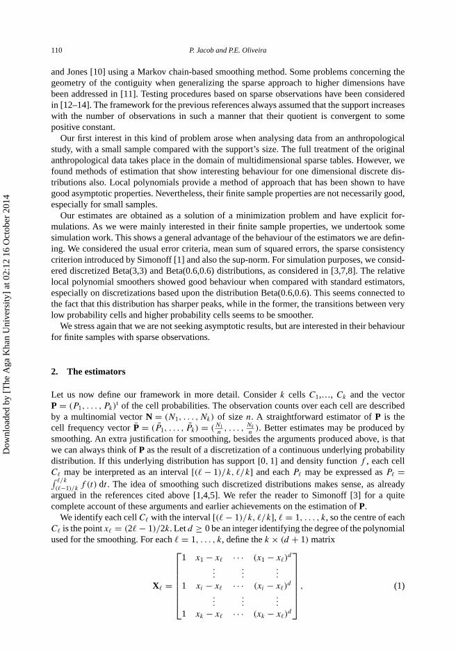
We identify each cell C� with the interval [(� − 1)/k, �/k], � = 1, . . . , k, so the centre of eachC� is the point x� = (2� − 1)/2k. Let d ≥ 0 be an integer identifying the degree of the polynomialused for the smoothing. For each � = 1, . . . , k, define the k × (d + 1) matrix

X� =

⎡⎢⎢⎢⎢⎢⎢⎣

1 x1 − x� · · · (x1 − x�)d

......

...

1 xi − x� · · · (xi − x�)d

......

...

1 xk − x� · · · (xk − x�)d

⎤⎥⎥⎥⎥⎥⎥⎦

, (1)

Dow

nloa

ded

by [

The

Aga

Kha

n U

nive

rsity

] at

02:

12 1

6 O

ctob

er 2

014

Journal of Statistical Computation and Simulation 111

and the k × k matrix

K� = diag

(1

hK

(x1 − x�

h

), . . . ,

1

hK

(xk − x�

h

)), (2)

where K is a symmetric density function with bounded support and h > 0. Let β� =(β0,�, . . . , βd,�)

t and, for each � = 1, . . . , k, β� the minimizer of

(P − X�β�)tK�(P − X�β�) = 1

h

k∑i=1

(Ni

n− β0,� − β1,�(xi − x�) − · · · − βd,�(xi − x�)

d

)2

× K

(xi − x�

h

). (3)

The estimator for P� is the constant term β0,� of β�. This is the local polynomial of degree d usedthroughout the literature, and we will denote it by PS(d) = (PS1(d), . . . , PSk(d)). The estimatorof the �th coordinate PS�(d) is representable as

∑kj=1 s�j Pj , where the s�j depend on the degree

d of the polynomial and on the cells C�, Cj . We refer to Aerts et al. [8] for an explicit expression.For a more general framework, where the design points are random, explicit expressions may befound in [15,16]. As local polynomial smoothers, these estimators automatically correct bordereffects at the cost of a somewhat more intricate expression for the coefficients s�j for the cells Cj

near the borders. The classification of a cell being near the border or in the interior depends on thesupport of the kernel K . As we shall explain next, the expression of the coefficients is simplifiedfor interior cells, so we will start by a precise definition of the interior cell.

We say that a cell C� is an interior cell if the support of K( · −x�

h) is a subset of [0, 1], i.e, if

K((x − x�)/h) = 0, whenever x �∈ [0, 1]. Otherwise, we say that C� is a border cell.For an interior cell C�, as the kernel K is supposed to be symmetric, the distribution of the

weights s�j is symmetrical with respect to x�. This is the source of the simplifications referred toearlier. For local polynomial smoothers of degrees d = 0, 1, and for interior cells, the symmetryimplies that the minimizer is the Nadaraya–Watson estimator, representable as

NW� = PS�(0) = PS�(1) =u∑

j=−u

Pj−�w(j), (4)

where

w(j) = K(j/kh)/

u∑i=−u

K(i/kh), j = −u, . . . , u.

For the local polynomial smoothers of degree d = 2, 3 and again for interior cells, therepresentation of the estimator is of the same form, just changing the weights. We have then

PS�(2) = PS�(3) =u∑

j=−u

Pj−�w∗(j) where w∗(j) = τ 4 − σ 2j 2

τ 4 − σ 4w(j), j = −u, . . . , u,

(5)

where σ 2, τ 4 are the second and fourth order moments of the following weight distribution w(·):

σ 2 =u∑

j=−u

j 2w(j) and τ 4 =u∑

j=−u

j 4w(j). (6)

Thus, the local polynomial smoothers of orders d = 2, 3 appear as kernel estimates associatedwith a redefined weight function w∗(·). This new weight function is still symmetric and it is

Dow

nloa

ded

by [

The

Aga

Kha

n U

nive

rsity

] at

02:

12 1

6 O

ctob

er 2

014

112 P. Jacob and P.E. Oliveira

easy to verify that∑u

j=−u j 2w∗(j) = 0, so this redefined weight function is a fourth order ker-nel. This means that this weight function w∗(·) may be negative, so the estimator PS(2) mayalso become negative for some cells C�. As we are trying to estimate probabilities, this is aninconvenient property.

We stress that those expressions apply only to interior cells. In this paper, we tried to avoidboundary modifications in comparing the estimators described earlier and those we will introducelater. So, instead of considering the expressions of the estimators as referred to in Aerts et al.[8], we used the well-known replication device of introducing fictitious cells C�, � = 1 − k, . . . , 0,to the left of the initial cells, and C�, � = k + 1, . . . , 2k, to the right [17]. The frequency in eachof these new cells is the one observed on the real cell, which is symmetrically situated withrespect to the origin or to the last original cell, respectively. That is, for the new cells, we defineP1−j = P2k+1−j = Pj , j = 1, . . . , k. For this enlarged support, we must redefine the matricesX� and K� allowing, the indexes to range from 1 − k to 2k. That is, X� is now the (3k) × (d + 1)

matrix with entries

X� =

⎡⎢⎢⎢⎢⎢⎢⎢⎢⎢⎢⎢⎢⎢⎢⎢⎣

1 x1−k − x� · · · (x1−k − x�)d

......

...

1 x0 − x� · · · (x0 − x�)d

1 x1 − x� · · · (x1 − x�)d

......

...

1 xk − x� · · · (xk − x�)d

1 xk+1 − x� · · · (xk+1 − x�)d

......

...

1 x2k − x� · · · (x2k − x�)d

⎤⎥⎥⎥⎥⎥⎥⎥⎥⎥⎥⎥⎥⎥⎥⎥⎦

, (7)

and K� becomes the (3k) × (3k) matrix

Kl = diag

(1

hK

(x1−k − x�

h

), . . . ,

1

hK

(x2k − x�

h

)). (8)

With this device, all the original cells become interior cells, so the formulas (4) and (5) apply to eachone of them. In order to introduce our estimators, it is convenient to define the (3k) × (3k) matrix

W� = diag

(K((xj − x�)/h)∑ki=1 K((xi − x�)/h)

, j = 1 − k, . . . , 2k

).

Note that the denominator in the entries of W� depends only on �. This matrix describes thesymmetric weights w(·) recentred at the cell C�, and it is simple to verify that the diagonal entriesare zero whenever |j − �| > u. Besides, remark that on Equation (3), replacing the matrices K�

by W� does not change the solution of the minimizing problem as β� = (Xt�K�X�)

−1Xt�K�P =

(Xt�W�X�)

−1Xt�W�P, because W and K are the same up to the multiplication by a constant.

Our goal is to achieve more precise approximations for small probabilities and, at the sametime, guarantee their positivity by minimizing expressions such as

H� = 1

β0,�

(P − X�β�)tW�(P − X�β�). (9)

Minimizing H� leads to arbitrarily negatively large values, as the function may be negative.We will minimize it on the orthant where βi,� > 0. This is a natural procedure with this errorfunction, as it becomes infinite whenever one of the βi,� is equal to 0. H� defines a relativeerror criterion, so we will call the derived estimator a relative local polynomial of degree d,

Dow

nloa

ded

by [

The

Aga

Kha

n U

nive

rsity

] at

02:

12 1

6 O

ctob

er 2

014

Journal of Statistical Computation and Simulation 113

denoted by RPS(d) = (RPS1(d), . . . , RPSk(d)). The idea of considering errors that are relative tothe probability we are trying to estimate is inspired on chi-square tests, and will contribute to someoverestimation of very small probabilities. This error function is, apart from the relativization of theerror, the same as considered for the local polynomial smoothers (3). However, the minimizationof Equation (9), for each � = 1, . . . , k, does not necessarily produce a probability distributionover the initial cells. So, we introduce this as a global condition and minimize the sum of theerrors H�. Thus our estimator appears as the solution of the optimization problem

minimizek∑

�=1

H�

subject tok∑

�=1

β0,� = 1.

Introducing the Lagrange multiplier, we need to minimize

H =k∑

�=1

H� + λ

(k∑

�=1

htβ� − 1

), (10)

where h = (1, 0, . . . , 0)t is a (d + 1) dimensional vector. We defer the computational details toAppendix 1. The estimator is, as before, the first coordinate of the minimizer of Equation (10)and may be expressed as

RPS�(d) =(P

t(W� − A�)P

)1/2

∑kj=1

(P

t(Wj − Aj )P

)1/2 , � = 1, . . . , k, (11)

where A� is a matrix to be described in Appendix 1 (see Equation (A6)). In order to give explicitexpressions for the square of the numerator of the relative local smoothers of degree d = 0, 1, 2, 3,we need, besides the second and fourth moments of the weight function (6) introduced before,the sixth moment and the corresponding convoluted moments,

γ 6 =u∑

j=−u

j 6w(j) and mt =u∑

j=−u

Pj−�jtw(j), t = 0, 1, 2, . . . .

Now we are able to produce explicit formulas for each value of the polynomial degree d.

• d = 0 : A� = 0, thus Pt(W� − A�)P = P

tW�P = ∑u

j=−u P 2j−�w(j);

• d = 1 : PtA�P = 1

σ 2 m21;

• d = 2 : PtA�P = 1

σ 2 m21 + 1

τ 4 m22;

• d = 3 : PtA�P = γ 6

σ 2γ 6−τ 8 m21 − 2τ 4

σ 2γ 6−τ 8 m1m3 + γ 6

σ 2γ 6−τ 8 m23 + 1

τ 4 m22.

Given an estimator P∗ = (P ∗1 , . . . , P ∗

k )t we consider three error criteria:

MSSE(P∗) = E

⎛⎝ k∑

j=1

(P ∗j − Pj )

2

⎞⎠ , NSUP(P∗) = sup

1≤j≤k

|P ∗j − Pj |,

SPSUP(P∗) = sup1≤j≤k

∣∣∣∣P∗j

Pj

− 1

∣∣∣∣ .

Dow

nloa

ded

by [

The

Aga

Kha

n U

nive

rsity

] at

02:

12 1

6 O

ctob

er 2

014

114 P. Jacob and P.E. Oliveira

MSSE is the usual L2 error, NSUP the sup-norm, while SPSUP, introduced by Simonoff [1],weights heavier the estimation of low probabilities, thus being a more sensitive criterion.

As will be evident when analysing simulation results, these relative local smoothers performwell when the distributions to be estimated have sharp peaks. When the discrete distribution hascells with probabilities changing in a smoother way, the sparse error criteria MSSE, SPSUP and,to a minor extent, NSUP, start showing a worse empirical behaviour than the local polynomialsmoothers NW or PS(2). This seems to be due to an overestimation of these probabilities.

3. Simulation results

We now report the comparative performance of the different local smoothers discussed above.As mentioned earlier, we discretized the Beta(3,3) and Beta(0.6,0.6) distributions over a givennumber of cells. In order to judge the influence of the sharpness of the peak, we also discretizedBeta(50,50) and, in a different direction, we shifted the discretization of Beta(0.6,0.6) and mixedsome of these shifted discretizations. Table 1 gives a description of the distributions used in thesimulation study. Each distribution was then discretized over 10, 50 or 100 cells, with 5, 25 or50 observations, respectively, for simulation purposes. We will report only results for the case ofdistributions over 50 cells (with 25 observations). The other cases showed a similar behaviourwhere the performance of the estimators is concerned. We computed the estimators for weightfunctions based on the Epanechnikov kernel discretized over a different number of cells, i.e.different bandwidths and also using a kernel based on a discretization of a Beta distribution.Estimation based on the Epanechnikov kernel generally produces better results, although in afew cases, the Beta kernels performed quite well. We report the results corresponding to bestobserved behaviour of the estimators. All numerical results included were obtained from 500simulated samples in each of the considered distribution. For benchmarking purposes we includethe performance of the HIST, the semiparametric estimator (FJ) proposed by Faddy and Jones [10]and the LL estimator proposed by Simonoff [3]. The HIST and the FJs are consistently worse thatthe local smoothers considered, FJ showing a better performance than the HIST. The LL generallyimproves somewhat on the local polynomial of degree 0, NW. For the more peaked distributionsconsidered, the relative polynomials can show a better performance than these estimators.

The choice of the number of points on the weight function, or the bandwidth to use a morecommon language, is not satisfactorily characterized for relative local smoothers. The manipula-tion of the mathematical expressions describing the estimators seems to be too complicated. Theempirical observation of the simulated results suggests that one could use the bandwidth derivedfor the local polynomials as a reference. The relative local polynomials of degrees 0 or 1 typicallyuse a little less points in the weight functions than the corresponding local polynomial of degree0. For relative local polynomial of degree 2, the results hint one should choose roughly half ofthe points considered for the local polynomial of degree 2. A more data-driven method for the

Table 1. Distributions used for discretization.

d1 Beta (3,3)d2 Beta (0.6,0.6)d3 S1/2(Beta (0.6,0.6))d4 S1/4(Beta (0.6,0.6))d5 0.3 × S1/4 (Beta (0.6,0.6)) + 0.7 × S1/2S1/4 (Beta (0.6,0.6))d6 0.2 × Inv(S1/4 (Beta (0.6,0.6))) + 0.5 × S1/2 (Beta (0.6,0.6)) + 0.3 × S1/4(Beta (0.6,0.6))d7 Beta (50,50)

Note: Sα , α ∈ [0, 1] denotes the shift of the kα first cells towards the final positions, Inv reversal of the order ofthe cells.

Dow

nloa

ded

by [

The

Aga

Kha

n U

nive

rsity

] at

02:

12 1

6 O

ctob

er 2

014

Journal of Statistical Computation and Simulation 115

number of points could be as follows: count the largest sequence of cells with zero observationsand enlarge by 2 or 4 this count, with an extra correction if it is even, to get the number of pointsto be used in the kernel. The idea behind this is that, as the support is known and has no zeroprobability cell, the kernel to be used should be able to look sufficiently far in order to constructa nonzero approximation for every cell. The enlargement proposed may seem somewhat subjec-tive, but the reported simulated behaviour is reasonable (see, for each of the local smoothers, theerrors reported in the second corresponding row in Tables 2–4). As can observed for the simulatedresults, the amount of smoothing to obtain optimal behaviour seems to be increasing accordingto error criterion used: MSSE, NSUP and SPSUP, on this order. So the enlargement consideredshould take into account which of the error criteria we want to prioritize. On the results reportedbelow, we used an enlargement by four points, as we were mainly concerned with MSSE.

The numerical results reported in Tables 2–4 are organized as follows: for each local smoother,the first line reports the simulated optimal mean value error, for the corresponding criteria togetherwith the optimal number of points for the weight function, i.e. the number of points for whichthe optimal mean value of the error is attained, given inside the parenthesis; on the second corre-sponding line, we report the error observed using the data-driven method described above for thechoice of the number of points on the weight function described above (also inside parenthesis).

Table 2. Simulated (×10−3) MSSE mean values and optimal number of points in the weight function (50 cells with25 observations).

d1 d2 d3 d4 d5 d6 d7

NW 1.5 (25) 4.8 (27) 4.6 (25) 4.7 (23) 3.2 (49) 1.9 (49) 7.4 (5)(1.5) (5.6) (5.2) (5.1) (4.4) (4.0) (75.4)

PS(2) 1.2 (49) 5.2 (49) 4.9 (49) 5.0 (43) 3.8 (45) 2.6 (49) 6.4 (9)(3.4) (9.3) (8.3) (8.1) (7.9) (7.8) (51.4)

RPS(0) 2.2 (17) 4.6 (19) 4.3 (17) 4.3 (17) 2.9 (27) 1.7 (45) 10.8 (3)(2.6) (4.7) (4.4) (4.3) (3.2) (2.7) (82.1)

RPS(1) 2.1 (19) 4.4 (19) 4.3 (19) 4.3 (17) 2.9 (27) 1.7 (45) 9.7 (3)(2.4) (4.5) (4.3) (4.3) (3.3) (2.7) (79.8)

RPS(2) 2.4 (21) 4.4 (21) 4.2 (21) 4.2 (19) 2.8 (29) 1.7 (49) 10.9 (7)(2.5) (4.8) (4.4) (4.3) (3.4) (3.0) (77.4)

LL 1.5 (23) 4.5 (25) 4.6 (27) 4.7 (19) 3.1 (49) 1.9 (49) 2.1 (7)(1.8) (5.2) (5.1) (5.0) (4.3) (3.9) (80.1)

HIST 38.1 38.7 39.3 38.6 39.4 39.7 34.3FJ 23.4 24.9 25.4 24.3 25.0 25.4 30.6

Table 3. Simulated (×10−3) NSUP mean values and optimal number of points in the weight function (50 cells with25 observations).

d1 d2 d3 d4 d5 d6 d7

NW 9.2 (25) 38.2 (11) 31.6 (11) 31.1 (9) 24.5 (13) 18.8 (31) 19.6 (7)(9.8) (38.1) (23.7) (32.1) (24.7) (20.7) (124.0)

PS(2) 8.3 (47) 38.4 (21) 31.7 (21) 31.3 (19) 24.7 (27) 18.3 (49) 23.7 (15)(16.3) (41.1) (33.7) (33.6) (30.2) (29.5) (97.7)

RPS(0) 11.7 (21) 39.8 (7) 31.9 (7) 31.2 (7) 24.2 (9) 19.1 (17) 27.1 (7)(12.2) (41.2) (35.9) (35.2) (25.1) (19.2) (128.9)

RPS(1) 11.5 (19) 38.8 (7) 32.0 (7) 31.4 (7) 24.4 (9) 19.1 (17) 20.9 (7)(12.1) (40.4) (35.5) (34.9) (25.0) (19.2) (127.5)

RPS(2) 12.2 (25) 39.5 (9) 32.4 (9) 31.7 (9) 24.3 (13) 19.0 (21) 27.6 (11)(12.7) (40.1) (34.3) (33.6) (24.5) (19.7) (125.9)

LL 9.9 (23) 37.4 (9) 31.5 (11) 31.0 (9) 24.4 (13) 18.7 (31) 19.6 (7)(10.4) (38.4) (32.7) (32.0) (24.6) (20.6) (124.0)

HIST 90.2 88.1 88.7 87.6 86.7 87.5 145.20FJ 68.3 70.8 69.9 68.7 67.7 68.0 110.9

Dow

nloa

ded

by [

The

Aga

Kha

n U

nive

rsity

] at

02:

12 1

6 O

ctob

er 2

014

116 P. Jacob and P.E. Oliveira

Table 4. Simulated SPUSP mean values and optimal number of points in the weight function (50 cells with 25observations).

d1 d2 d3 d4 d5 d6

NW 11.65 (3) 0.69 (33) 0.66 (37) 0.71 (27) 0.66 (49) 0.54 (49)(87.4) (0.95) (0.99) (0.97) (0.99) (0.98)

PS(2) 13.24 (5) 0.73 (49) 0.74 (49) 0.77 (45) 0.76 (47) 0.66 (49)(56.4) (1.55) (1.60) (1.59) (1.58) (1.59)

RPS(0) 13.33 (3) 0.69 (23) 0.65 (29) 0.65 (25) 0.62 (25) 0.51 (37)(134.1) (0.77) (0.76) (0.75) (0.75) (0.74)

RPS(1) 12.05 (3) 0.68 (23) 0.65 (29) 0.65 (25) 0.62 (25) 0.51 (39)(138.9) (0.78) (0.79) (0.77) (0.77) (0.77)

RPS(2) 15.64 (3) 0.68 (27) 0.64 (33) 0.64 (29) 0.61 (31) 0.51 (47)(130.8) (0.89) (0.88) (0.87) (0.86) (0.86)

LL 12.21 (3) 0.67 (27) 0.66 (35) 0.74 (49) 0.65 (49) 0.54 (47)(92.9) (0.90) (0.96) (0.96) (0.97) (0.96)

HIST 15.64 4.76 4.97 4.80 4.65 4.66FJ 12.44 3.61 3.86 3.70 3.62 3.61

Naturally, for the HIST and FJ estimators, we report only the simulated error value, as there isno smoothing involved. For example, for distribution d3, the estimator RPS(2) produces a meanvalue for the MSSE equal to 4.2 × 10−3, this is the best mean value for the MSSE when smooth-ing based on different support sizes for the weighting function, and is obtained by choosing aweight function with 21 points in its support. If, for each run, we apply the data-driven method forchoosing the weight function, we get a mean value for the MSSE equal to 4.4 × 10−3. One thingthat is immediately apparent is that the data-driven method gets us quite close to the optimal meanbehaviour of the estimator. The one exception is distribution d7, which has a very sharp peak andis almost null away from that peak, implying a rather large number of cells with no observation.

Table 2 reports the behaviour of the simulated MSSE values. The relative local smoothers showthe best performance for distributions d2 to d6, i.e. those distributions that are constructed fromthe Beta(0.6,0.6) discretization. This behaviour is confirmed if we look at the performance withrespect to NSUP error, as showed by the simulated results reported in Table 3. There is a lossof performance of the relative local smoothers on distribution d2 but a gain on distribution d7,indicating that, as far as this error is concerned, the peaks should not be too sharp. Finally, withrespect to the SPUSP criterion, reported in Table 4 (there are no results on distribution d7, as thecell probabilities are too close to zero so the quotients involved in the definition of SPUSP producecomputational errors), this general trend is confirmed, the local polynomial or the LL estimatorbeing preferable only for distribution d1, the smoothest of the considered distributions. Thevariability of the simulated values for the error criteria showed that the relative local polynomialsgenerally have more stable behaviour than the local polynomials.

In order to have a clearer view of the compared performance of each estimator, we looked at thenumber of times each one produced the best error for each of the distributions and criteria. We donot include results on the HIST or the FJ estimator, as these consistently produced relatively poorapproximations. In Table 5 we report, for each criteria and distribution, the two best estimators,indicating the percentage of best simulated error registered. For example, for distribution d5, theestimator RPS(2) had the best MSSE error in 62.8% of the simulated samples, while NW showedthe best MSSE error in 20.2% of the simulated samples. These results confirm the impressionobtained from the simulated mean errors. For the MSSE criterion we should prefer the RPS(2)estimator, except for the smoother distributions d1 and d7. As for the NSUP, the mean simulatedvalues gave an impression of equivalent performance of the estimators with a slight advantage ofLL, not confirmed here. This is an indication of more variability for PS(2), which seems to performbetter on this comparison. The loss on the mean performance can only be explained by a larger

Dow

nloa

ded

by [

The

Aga

Kha

n U

nive

rsity

] at

02:

12 1

6 O

ctob

er 2

014

Journal of Statistical Computation and Simulation 117

Table 5. Comparative performance of the estimators: percentage of best performance for simulated samples.

MSSE NSUP SPSUP

d1 PS(2): 81.6% NW, PS(1): 6.2% PS(2): 70.0% NW: 18.2% NW: 54.4% RPS(0): 37.2%d2 RPS(2): 44.8% LL: 33.2% PS(2): 31.4% NW: 23.6% PS(2): 26.6% NW: 20.0%d3 RPS(2): 54.2% LL: 18.2% PS(2): 27.4% NW: 20.0% PS(2): 34.0% NW: 18.0%d4 RPS(2): 58.6% LL: 16.2 % PS(2): 23.6% NW: 23.2% PS(2): 24.2% RPS(2): 20.0%d5 RPS(2): 62.8% NW: 20.2% PS(2): 26.0% NW: 18.2% NW: 22.2% RPS(1): 18.4%d6 RPS(2): 41.4% NW: 14.2% PS(2): 43.4% NW: 16.6% RPS(0): 26.8% PS(2): 22.4%d7 LL: 91.4% RPS(2): 4.0% NW: 52.0% RPS(1): 31.4%

Table 6. Comparative performance of the estimators: percentage of best performance for simulated samples using datadriven bandwidth choice.

MSSE NSUP SPSUP

d1 NW: 77.2% RPS(1), RPS(2): 4.8% NW: 70.8% PS(2): 7.8% HIST: 97.8% NW: 1.4%d2 RPS(1): 33.4% RPS(2): 29.6% PS(2): 37.0% NW: 36.0% RPS(0): 42.8% RPS(1): 34.4%d3 RPS(2): 42.6% RPS(1): 19.8% PS(2): 49.2% NW: 30.4% RPS(0): 55.2% RPS(1): 23.4%d4 RPS(2): 40.6% RPS(1): 20.0 % PS(2): 43.2% NW: 35.2% RPS(0): 45.2% RPS(1): 23.6%d5 RPS(0): 39.4% RPS(1): 26.0% NW: 32.8% PS(2): 17.0% RPS(0): 61.0% RPS(1): 20.4%d6 RPS(0): 55.2% RPS(1): 24.0% NW: 26.2% RPS(1): 23.8% RPS(0): 64.0% RPS(1): 20.2%d7 HIST: 67.4% PS(2): 32.6% PS(2): 85.6% HIST: 14.4% LL: 19.6% RPS(1): 16.4%

variability. Finally, with respect to SPUSP, the relative smoothers lose in the aspect, indicatingagain a larger variability of the performance of the local polynomial smoothers that perform worsewhen we look at the simulated mean value for SPUSP. In Table 6, we report the same kind ofinformation for the estimators using the data-driven bandwidth choice that is proposed above. Therelative smoothers are most commonly the best ones, except for the smoother distributions d1and d7, thus confirming the general impression we have been collecting. It should be mentionedthat there is a clear change in the estimators with respect to the SPSUP criterion. This could beexplained taking into account our comments on the bandwidth choice method we used. The extracorrection on the number of points after counting sequences of consecutive empty cells shouldbe larger if we want SPSUP to prevail. The results reported had the MSSE criterion in mind.

4. An application

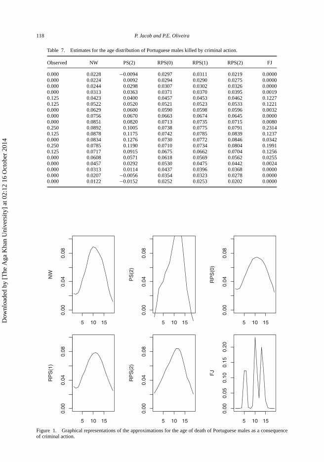
The data of the anthropological study considered a series of people who had been killed as aconsequence of a criminal action. The data treated males and females differently and aimed,among other features, to produce an estimate of the probability of a person being subjected toa criminal action resulting in his/her death. There were records for eight Portuguese males andtheir ages at moment of death, classified into 19 age intervals, as reported in the first column ofTable 7. We computed estimates for the age distribution at moment of death using the differentestimators. The FJ [10] estimator is quite sensitive to the choice of a reference distribution. Herewe show the estimates produced by using as reference measure the age distribution of the entirePortuguese population. The local polynomial of degree 2 still produces some negative estimatesfor the probability of a few tail cells. The estimates produced by NW, RPS(0) and RPS(1) seem tocapture a better picture of what was expected by the anthropological experts, although they tend tooverestimate what could be expected at both tails of the distribution. A graphical representation ofthese approximations is given in Figure 1 (note that the vertical scale for the Faddy and Jones [10]is larger).

Dow

nloa

ded

by [

The

Aga

Kha

n U

nive

rsity

] at

02:

12 1

6 O

ctob

er 2

014

118 P. Jacob and P.E. Oliveira

Table 7. Estimates for the age distribution of Portuguese males killed by criminal action.

Observed NW PS(2) RPS(0) RPS(1) RPS(2) FJ

0.000 0.0228 −0.0094 0.0297 0.0311 0.0219 0.00000.000 0.0224 0.0092 0.0294 0.0290 0.0275 0.00000.000 0.0244 0.0298 0.0307 0.0302 0.0326 0.00000.000 0.0313 0.0363 0.0371 0.0370 0.0395 0.00190.125 0.0423 0.0400 0.0457 0.0453 0.0462 0.12270.125 0.0522 0.0520 0.0521 0.0523 0.0533 0.12210.000 0.0629 0.0600 0.0590 0.0598 0.0596 0.00320.000 0.0756 0.0670 0.0663 0.0674 0.0645 0.00000.000 0.0851 0.0820 0.0713 0.0735 0.0715 0.00800.250 0.0892 0.1005 0.0738 0.0775 0.0791 0.23140.125 0.0878 0.1175 0.0742 0.0785 0.0839 0.12370.000 0.0834 0.1276 0.0730 0.0772 0.0846 0.03420.250 0.0785 0.1190 0.0710 0.0734 0.0804 0.19910.125 0.0717 0.0915 0.0675 0.0662 0.0704 0.12560.000 0.0608 0.0571 0.0618 0.0569 0.0562 0.02550.000 0.0457 0.0292 0.0530 0.0475 0.0442 0.00240.000 0.0313 0.0114 0.0437 0.0396 0.0368 0.00000.000 0.0207 −0.0056 0.0354 0.0323 0.0278 0.00000.000 0.0122 −0.0152 0.0252 0.0253 0.0202 0.0000

0.00

0.04

0.08

RP

S(1

)

0.00

0.04

0.08

NW

0.00

0.04

0.08

PS

(2)

0.00

0.04

0.08

RP

S(0

)

0.00

0.04

0.08

RP

S(2

)

5 10 15

5 10 15 5 10 15 5 10 15

5 10 15 5 10 15

0.00

0.05

0.10

0.15

0.20

FJ

Figure 1. Graphical representations of the approximations for the age of death of Portuguese males as a consequenceof criminal action.

Dow

nloa

ded

by [

The

Aga

Kha

n U

nive

rsity

] at

02:

12 1

6 O

ctob

er 2

014

Journal of Statistical Computation and Simulation 119

References

[1] J. Simonoff, A penalty function approach to smoothing large sparse contingency tables, Ann. Statist. 11 (1983),pp. 208–218.

[2] J. Simonoff, Smoothing categorical data, J. Statist. Plann. Inference 47 (1995), pp. 41–69.[3] J. Simonoff, Smoothing Methods in Statistics, Springer-Verlag, New York, 1996.[4] P. Burman, Smoothing sparse contingency tables, Sankhya Ser. A 49 (1987), pp. 24–36.[5] P. Hall and D. Titterington, On smoothing sparse multinomial data, Austral. J. Statist. 29 (1987), pp. 19–37.[6] J. Dong and J. Simonoff, A geometric combination estimator for d-dimensional ordinal contingency tables, Ann.

Statist. 23 (1995), pp. 1143–1153.[7] M. Aerts, I. Augustyns, and P. Janssen, Local polynomial estimation of contingency table cell probabilities, Statistics

30 (1997), pp. 127–148.[8] M. Aerts, I. Augustyns, and P. Janssen, Sparse consistency and smoothing for multinomial data, Statist. Probab. Lett.

33 (1997), pp. 41–48.[9] M.Aerts, I.Augustyns, and P. Janssen, Central limit theorem for the total squared error of local polynomial estimators

of cell probabilities, J. Statist. Plann. Inference 91 (2000), pp. 181–193.[10] M. Faddy and M. Jones, Semiparametric smoothing for discrete data, Biometrika 85 (1998), pp. 131–138.[11] P. Hall, B. Seifert, and B. Turlach, On adaptation to sparse design in bivariate local linear regression, J. Korean

Math. Soc. 30 (2001), pp. 231–246.[12] H. Liero, L2-tests for sparse multinomials, Statist. Probab. Lett. 5 (2001), pp. 147–158.[13] P. Burman, On some testing problems for sparse contingency tables, J. Multivariate Anal. 88 (2004), pp. 1–18.[14] J. Baek, Goodness-of-fit test using local maximum likelihood polynomial estimator for sparse multinomial data,

J. Korean Math. Soc. 33 (2004), pp. 313–321.[15] D. Ruppert and M. Wand, Multivariate locally weighted least squares regression, Ann. Statist. 22 (1994),

pp. 1346–1370.[16] J. Fan and I. Gijbels, Local Polynomial Modelling and its Applications, Chapman & Hall, London, 1997.[17] E. Schuster, Incorporating support constraints into nonparametric estimators of densities, Comm. Statist. A Theory

Methods 14 (1985), pp. 1123–1136.

Appendix 1. Derivation of the RPS estimators

We start by computing the derivative of H , given by Equation (10), with respect to the polynomial parameters in eachcell, i.e. with respect to β�, � = 1, . . . , k. This gives rise to the following system of (d + 1) equations:

−2Xt�W�(P − X�β�) − h

β0,�

(P − X�β�)tW�(P − X�β�) = −λβ0,�h. (A1)

Remark that only the first of these equations is nonlinear. Let us start by solving the linear part of this system of equations.For this purpose define β� = β� − β0,�h and X�, the (d + 1) column matrix obtained from X� by replacing its first columnentries by zeros. Then,

X�β� = X�β� + β0,�e, (A2)

where e = (1, . . . , 1)t , and the linear part of Equation (A1) may be rewritten as

Xt�W�(P − β0,�e) = X

t�W�X�β�.

Now the matrix Xt�W�X� has a first line and column with all entries equal to zeros. The remaining entries define a square

block M. Whenever this block M is nonsingular, we shall say the matrix has a generalized inverse and write

(X

t�W�X�

)←− =⎡⎢⎣

0 · · · 0... M−1

0

⎤⎥⎦ .

With this remark, we have that

β� =(X

t�W�X�

)←−X

t�W�(P − β0,�e). (A3)

Now we go back to the first equation of the system of equations (A1). To isolate this equation, we multiply the system ofequations (A1) by β0,�ht . Using Equation (A2), it follows that

(P − X�β� + β0,�e

)tW�

(P − X�β� − β0,�e

)= λβ2

0,�.

Dow

nloa

ded

by [

The

Aga

Kha

n U

nive

rsity

] at

02:

12 1

6 O

ctob

er 2

014

120 P. Jacob and P.E. Oliveira

Expanding and noting that etW�e = 1, the previous equation is equivalent to

(P − X�β�

)tW�

(P − X�β�

)− β2

0,� = λβ20,�. (A4)

Now we replace β� using Equation (A3) to find, after some simplification,

Pt(W� − A�) P − β2

0,�et (W� − A�) e = λβ20,�, (A5)

where

A� = Wt�X�

(X

t�W�X�

)←−X

t�W�. (A6)

For some explicit computation of A�, refer to Appendix 2. Now the replication device we described earlier comes intoaction: etA�e does not depend on �, due to the fact that we always deal with interior cells.

Before continuing the analysis we note a useful fact: if we remove the constraint∑k

�=1 β0,� = 1, which is equivalentto setting λ = 0, we find that

Pt(W� − A�) P = β2

0,�et (W� − A�) e,

thus the random variable Pt(W� − A�)P has, for each � = 1, . . . , k, the same sign as et(W� − A�)e = 1 − etA�e, which

is constant for the cells C�, � = 1, . . . , k. We prove, in Appendix 2, that for d = 0, 1, 2, 3, et(W� − A�)e > 0. Thus, ford = 0, 1, 2, 3, it follows from Equation (A5), that

β20,�

(λ + et (W� − A�) e

)> 0.

Finally, taking into account that β0,�, being an estimator for a probability, should be positive,

β0,� =(P

t(W� − A�) P

)1/2

(λ + et (W� − A�) e

)1/2 . (A7)

Using the constraint to the optimization problem, we find that

(λ + et (W� − A�) e

)1/2 =k∑

j=1

(P

t (Wj − Aj

)P)1/2

.

From this equation and Equation (A7), the expression (11) for RPS(d) follows.It remains to verify that we have indeed identified a minimum. First remark that, as the constraint is linear in β�, the

term corresponding to the Lagrange multiplier does not appear in the Hessian matrix of H . This implies that ∇2H is a blockdiagonal matrix with blocks defined by the Hessian matrices of each H�. It is now easy to check that, for u = (u1| . . . |uk)

a general k×(d + 1) vector, we have

ut∇2Hu =k∑

�=1

ut�∇2H�u� = 2

k∑�=1

1

β0,�

Zt�Z� ≥ 0,

where Z� = u0,�

β0,�W1/2

� (P − X�β�) + W1/2� X�u�. As the objective function and the constraint are convex, the Karush–

Kuhn–Tucker conditions ensure we have, in fact, a minimum.

Appendix 2. Explicit computation of A�

We give brief indications about the explicit computation of A� for the cases d = 1, 2, 3 and verify that, for these valuesof d, et(W� − A�)e > 0. Given α ∈ N, define

Sα =u∑

j=−u

(x� − x�+j )αw(j) =

u∑j=−u

jα

kαw(j).

It follows by symmetry that S1 = S3 = S5 = 0. As for the even values of α,

S2 = σ 2

k2, S4 = τ 4

k4, S6 = γ 6

k6.

Dow

nloa

ded

by [

The

Aga

Kha

n U

nive

rsity

] at

02:

12 1

6 O

ctob

er 2

014

Journal of Statistical Computation and Simulation 121

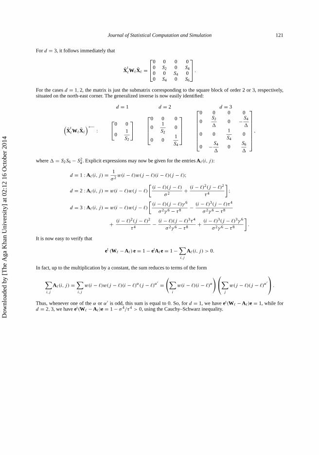
For d = 3, it follows immediately that

Xt�W�X� =

⎡⎢⎣

0 0 0 00 S2 0 S40 0 S4 00 S4 0 S6

⎤⎥⎦ .

For the cases d = 1, 2, the matrix is just the submatrix corresponding to the square block of order 2 or 3, respectively,situated on the north-east corner. The generalized inverse is now easily identified:

d = 1 d = 2 d = 3

(X

t�W�X�

)←− :⎡⎣0 0

01

S2

⎤⎦

⎡⎢⎢⎢⎣

0 0 0

01

S20

0 01

S4

⎤⎥⎥⎥⎦

⎡⎢⎢⎢⎢⎢⎢⎢⎣

0 0 0 0

0S2

0 −S4

0 01

S40

0 −S4

0

S6

⎤⎥⎥⎥⎥⎥⎥⎥⎦

,

where = S2S6 − S24 . Explicit expressions may now be given for the entries A�(i, j):

d = 1 : A�(i, j) = 1

σ 2w(i − �)w(j − �)(i − �)(j − �);

d = 2 : A�(i, j) = w(i − �)w(j − �)

[(i − �)(j − �)

σ 2+ (i − �)2(j − �)2

τ 4

];

d = 3 : A�(i, j) = w(i − �)w(j − �)

[(i − �)(j − �)γ 6

σ 2γ 6 − τ 8− (i − �)3(j − �)τ 4

σ 2γ 6 − τ 8

+ (i − �)2(j − �)2

τ 4− (i − �)(j − �)3τ 4

σ 2γ 6 − τ 8+ (i − �)3(j − �)3γ 6

σ 2γ 6 − τ 8

].

It is now easy to verify that

et (W� − A�) e = 1 − etA�e = 1 −∑i,j

A�(i, j) > 0.

In fact, up to the multiplication by a constant, the sum reduces to terms of the form

∑i,j

A�(i, j) =∑i,j

w(i − �)w(j − �)(i − �)α(j − �)α′ =

(∑i

w(i − �)(i − �)α

)⎛⎝∑

j

w(j − �)(j − �)α′⎞⎠ .

Thus, whenever one of the α or α′ is odd, this sum is equal to 0. So, for d = 1, we have et(W� − A�)e = 1, while ford = 2, 3, we have et(W� − A�)e = 1 − σ 4/τ 4 > 0, using the Cauchy–Schwarz inequality.

Dow

nloa

ded

by [

The

Aga

Kha

n U

nive

rsity

] at

02:

12 1

6 O

ctob

er 2

014