arX

iv:1

303.

2899

v1 [

gr-q

c] 1

2 M

ar 2

013

Relativistic Kinetic Theory: An IntroductionOlivier Sarbach and Thomas Zannias

Instituto de Física y Matemáticas, Universidad Michoacanade San Nicolás de HidalgoEdificio C-3, Ciudad Universitaria, 58040 Morelia, Michoacán, México.

Abstract. We present a brief introduction to the relativistic kinetictheory of gases with emphasison the underlying geometric and Hamiltonian structure of the theory. Our formalism starts witha discussion on the tangent bundle of a Lorentzian manifold of arbitrary dimension. Next, weintroduce the Poincaré one-form on this bundle, from which the symplectic form and a volume formare constructed. Then, we define an appropriate Hamiltonianon the bundle which, together with thesymplectic form yields the Liouville vector field. The corresponding flow, when projected ontothe base manifold, generates geodesic motion. Whenever theflow is restricted to energy surfacescorresponding to a negative value of the Hamiltonian, its projection describes a family of future-directed timelike geodesics. A collisionless gas is described by a distribution function on suchan energy surface, satisfying the Liouville equation. Fibre integrals of the distribution functiondetermine the particle current density and the stress-energy tensor. We show that the stress-energytensor satisfies the familiar energy conditions and that both the current and stress-energy tensor aredivergence-free.

Our discussion also includes the generalization to chargedgases, a summary of the Einstein-Maxwell-Vlasov system in any dimensions, as well as a brief introduction to the general relativisticBoltzmann equation for a simple gas.

Keywords: general relativity, kinetic theory, Einstein-Maxwell-Vlasov systemPACS: 04.20.-q,04.25.-g,04.40.-b

INTRODUCTION

Kinetic theory of gases is an old subject with rich history. Its acceptance as a scien-tific theory with potential predictive power marked the revival of the atomic theory ofnature proposed by Democritus and Leucippus in the ancient time. As early as 1738,Daniel Bernoulli proposed that gases consist of a great number of molecules movingin all directions and the notion of pressure is a manifestation of their kinetic energy ofmotion. Gradually, the idea of Bernoulli developed furtherculminating in the formula-tion of the Maxwellian distribution of molecular velocities and the Maxwell-Boltzmanndistribution at the end of the 19th century.1

The arrival of the 20th century marks a new era for kinetic theory. Einstein’s funda-mental 1905 paper on Brownian motion establishes the atomicstructure of matter, andmoreover the birth of special relativity set new challengesin re-formulating kinetic the-ory and its close relative thermodynamics, so that they are Poincaré covariant theories.As early as 1911, Jüttner treated the equilibrium state of a special relativistic gas [2, 3, 4]while early formulations of (special) relativistic kinetic theory and relativistic thermo-

1 For historical facts regarding the early development of kinetic theory see Ref. [1].

dynamics, successes, failures as well as early references can be found in the books byPauli [5] and Tolman [6].

Synge in 1934 [7] (see also [8]) introduced the notion of the world lines of gasparticles as the most fundamental ingredient for the description of a relativistic gas,and this idea led to the development of the modern generally covariant formulationof relativistic kinetic theory. Synge’s idea led naturallyto the notion of the invariantdistribution function and a statistical description of a relativistic gas which is fullyrelativistic.

The period after 1960 characterizes the modern developmentof relativistic kinetictheory based on the relativistic Boltzmann equation, and anearly treatment can be foundin the paper by Tauber and Weinberg [9]. An important contribution to the subjectwas the work by Israel [10] where conservation laws and the relativistic version ofthe H-theorem is presented and the important notion of the state of thermodynamicalequilibrium in a gravitational field is clarified. Further ithas been recognized in [10]that a perfect gas has a bulk viscosity, a purely relativistic effect. Gradually, with thediscovery of the cosmic microwave background radiation, pulsars and quasars it hasbecome evident that relativistic flows of matter are not any longer just mathematicalcuriosities but they are of relevance to astrophysics and early cosmology as well. Thesenew discoveries led to further studies of relativistic kinetic theory and the formulationof the transient thermodynamics [11, 12, 13, 14, 15, 16]. Thedevelopment of black holephysics and the realization that their interaction with therest of the universe requires afully general relativistic treatment, promoted relativistic kinetic theory to an importantbranch of relativistic astrophysics and cosmology. For an overview, see the recent bookby Cercignani and Kremer [17].

The formulation of the Cosmic Censorship Hypothesis (CSH) led to the search ofmatter models that go beyond the traditional fluids or magneto-fluids, and here studiesof the Einstein-Liouville, Einstein-Maxwell-Vlasov and Einstein-Boltzmann equationsare very relevant and on the frontier of studies in mathematical relativity, see for instanceRefs. [18, 19, 20, 21] and Ref. [22] for a recent review.

The strong cosmic censorship hypothesis affirms that the maximal Cauchy develop-ment of generic initial data for the Einsteins equations should be an inextendible space-time. Since this development is the largest region of the spacetime which is uniquelydetermined by the initial data, CSH affirms that the time evolution of a spacetime canbe generically fixed by giving initial data. In any study of the CSH the choice of thematter model is very important. For instance, dust and perfect fluid models may lead tothe formation of shell crossing singularities and shocks even in the absence of gravity.Their formation obscures a clear understanding of the global spacetime structure associ-ated to the gravitational singularities. Kinetic theory offers a good candidate for a mattermodel that avoids these problems. Studies of solutions of the Einstein-Liouville systemare characterized by a number of encouraging properties, see for instance [23] and [22].

Motivated by the above considerations, in this work we present a modern introductionto relativistic kinetic theory. Our work is mainly based on Synge’s ideas and early workby Ehlers [24], however, in contrast to their work, we derivethe relevant ingredientsof the theory using a Hamiltonian formulation. As will become evident further ahead,our approach exhibits transparently the basic ingredientsof the theory and leads togeneralizations.

In this work, (M,g) denotes aC∞-differentiable Lorentzian manifold of dimensionn= 1+d, with the signature convention(−,+,+, . . . ,+) for the metricg. Greek indicesµ,ν,σ , . . . run from 0 tod while Latin indicesi, j,k, . . . run from 1 tod, and we use theEinstein summation convention.X (N) andΛk(N) denote the class ofC∞ vector andk-form fields on a differentiable manifoldN, while iX and£X denote the interior productand the Lie derivative with respect to the vector fieldX.

THE TANGENT BUNDLE

In this section we begin with the definition of the tangent bundle and summarize someof its most important properties. LetTxM denote the vector space of all tangent vectorsp at some eventx∈ M. The tangent bundle ofM is defined as

TM := (x, p) : x∈ M, p∈ TxM,

with the associated projection mapπ : TM → M, (x, p) 7→ x. The fibre atx∈ M is thespaceπ−1(x) = (x,TxM), and thus, it is isomorphic toTxM.

Lemma 1. TM is an orientable,2n-dimensional C∞-differentiable manifold.

Remark: Notice thatTM is orientable regardless whetherM is oriented or not.

Proof. The proof is based on the observation that a local chart(U,φ) of M defines in anatural way a local chart(V,ψ) as follows. LetV := π−1(U) and define

ψ : V → φ(U)×Rn ⊂ R

2n,

(x, p) 7→(

x0,x1, . . . ,xd, p0, p1, . . . , pd)

:=(

φ(π(x, p)),dx0x(p),dx1

x(p), . . . ,dxdx(p)

)

.

By taking an atlas(Uα ,φα) of M, the corresponding local charts(Vα ,ψα) coverTM.Furthermore, one can verify that the transition functions areC∞-differentiable and thattheir Jacobian matrix have positive determinant, yieldingan oriented atlas ofTM.

We call the local coordinates(x0,x1, . . . ,xd, p0, p1, . . . , pd) adapted local coordinates,

and

∂∂x0

∣

∣

∣

(x,p), . . . , ∂

∂ pd

∣

∣

∣

(x,p)

and

dx0(x,p), . . . ,dpd

(x,p)

are the corresponding basis of

the tangent and cotangent spaces ofTM at(x, p). Any tangent vectorL ∈ T(x,p)(TM) canthen be expanded as

L = Xµ ∂∂xµ

∣

∣

∣

∣

(x,p)+Pµ ∂

∂ pµ

∣

∣

∣

∣

(x,p), Xµ = dxµ

(x,p)(L), Pµ = dpµ(x,p)(L).

Likewise, a cotangent vectorω ∈ T∗(x,p)(TM) can be expanded as

ω = αµ dxµ |(x,p)+βµ dpµ |(x,p) , αµ = ω

(

∂∂xµ

∣

∣

∣

∣

(x,p)

)

, βµ = ω

(

∂∂ pµ

∣

∣

∣

∣

(x,p)

)

.

The projection mapπ : TM → M induces a projectionπ∗(x,p) : T(x,p)(TM) → TxMthrough the push-forward ofπ , defined asπ∗(x,p)(L)[g] := L[gπ ] for a tangent vectorLin T(x,p)(TM) and a functiong : M →R which is differentiable atx. It is a simple matterto verify that

π∗(x,p)

(

∂∂xµ

∣

∣

∣

∣

(x,p)

)

=∂

∂xµ

∣

∣

∣

∣

x, π∗(x,p)

(

∂∂ pµ

∣

∣

∣

∣

(x,p)

)

= 0, (1)

and thus, the projection of an arbitrary vector fieldL ∈ X (TM) on TM is given by

π∗(x,p)(L(x,p)) = Xµ(x, p)∂

∂xµ

∣

∣

∣

∣

x, L(x,p) = Xµ(x, p)

∂∂xµ

∣

∣

∣

∣

(x,p)+Pµ(x, p)

∂∂ pµ

∣

∣

∣

∣

(x,p),

in adapted local coordinates.For the following, we consider a differentiable curveγ : I → M,λ 7→ γ(λ ) on M. It

induces a parameter-dependentlift which is defined in the following way:

γ : I → TM, λ 7→ γ(λ ) :=

(

γ(λ ),d

dλγ(λ )

)

.

Sinceπ γ = γ it follows immediately that the tangent vectorsX andX of γ andγ arerelated to each other byπ∗(X) = X. In adapted local coordinates(xµ , pµ) we can expand

Xγ(λ ) = Xµ(λ )∂

∂xµ

∣

∣

∣

∣

γ(λ ), Xγ(λ ) = Xµ(λ )

∂∂xµ

∣

∣

∣

∣

γ(λ )+Pµ(λ )

∂∂ pµ

∣

∣

∣

∣

γ(λ ),

where the coefficients are given by

Xµ(λ ) = xµ(λ ), Pµ(λ ) = xµ(λ ),

wherexµ(λ ) parametrizes the curveγ in the local chart(U,φ) of the base manifold, anda dot denotes differentiation with respect toλ .

As a particular example of this lift, consider the trajectory γ : I → M of a particle ofmassm> 0 and chargeq in an external electromagnetic fieldF ∈ Λ2(M). The equationsof motion are

∇pp= qF(p), p :=d

dλγ(λ ), (2)

whereF : X (M)→ X (M) is defined byg(X, F(Y)) = F(X,Y) for all X,Y ∈ X (M),andλ is an affine parameter, normalized2 such thatg(p, p) =−m2. Consider the tangentvectorL to the associated liftγ : I → TM. Since in adapted local coordinates ˙xµ = pµ

and pµ =−Γµαβ pα pβ +qFµ

ν pν , we find

L(x,p) = pµ ∂∂xµ

∣

∣

∣

∣

(x,p)+[

qFµν(x)p

ν −Γµαβ (x)p

α pβ] ∂

∂ pµ

∣

∣

∣

∣

(x,p), (3)

2 Notice that Eq. (2) implies thatg(p, p) is constant along the trajectories, due to the antisymmetryof F .

and thisL defines a vector field onγ. By extending this construction to arbitrary curvesone obtains a vector fieldL on TM, called theLiouville vector field. In the next section,we shall provide an alternative definition of the Liouville vector field based on Hamilto-nian mechanics.

HAMILTONIAN DYNAMICS ON THE TANGENT BUNDLE

The purpose of this section is twofold. At first, we introducea symplectic structureon the tangent bundle which in turn is the backbone of our formulation of kinetictheory. Secondly, we introduce a natural Hamiltonian function onTM whose associatedHamiltonian vector fieldL coincides with the Liouville vector field defined in Eq. (3).Moreover, the symplectic structure defines a natural volumeform onTM which will behelpful to set up integration onTM.

In order to define the symplectic structure, we note that the spacetime metricg inducesa natural one-formΘ ∈ Λ1(TM) on the tangent bundle, called thePoincaré or theLioville one-form. It is defined as

Θ(x,p)(X) := gx(p,π∗(x,p)(X)), X ∈ T(x,p)(TM), (4)

at an arbitrary point(x, p) ∈ TM. In terms of adapted local coordinates(xµ , pν) we mayexpand

X = Xµ ∂∂xµ

∣

∣

∣

∣

(x,p)+Yν ∂

∂ pν

∣

∣

∣

∣

(x,p), π∗(x,p)(X) = Xµ ∂

∂xµ

∣

∣

∣

∣

x, p= pµ ∂

∂xµ

∣

∣

∣

∣

x,

and obtainΘ(x,p) = gµν(x)p

µ dxν |(x,p) , (5)

which shows thatΘ is C∞-differentiable. The symplectic formΩs on TM is defined asthe two-form

Ωs := dΘ, (6)

which is closed. In adapted local coordinates we obtain fromEq. (5),

Ωs= gµν(x) dpµ ∧dxν |(x,p)+∂gµν

∂xα (x)pµ dxα ∧dxν |(x,p) . (7)

The following proposition shows thatΩs induces a natural volume form onTM, andthus it is non-degenerated.

Proposition 1. The n-fold product3

Λ :=(−1)

n(n−1)2

n!Ωs∧Ωs∧ . . .∧Ωs∈ Λ2n(TM) (8)

satisfiesΛ(x,p) 6= 0 for all (x, p) ∈ TM, and thus defines a volume form on TM.

3 The choice for the normalization ofΛ will become clear later.

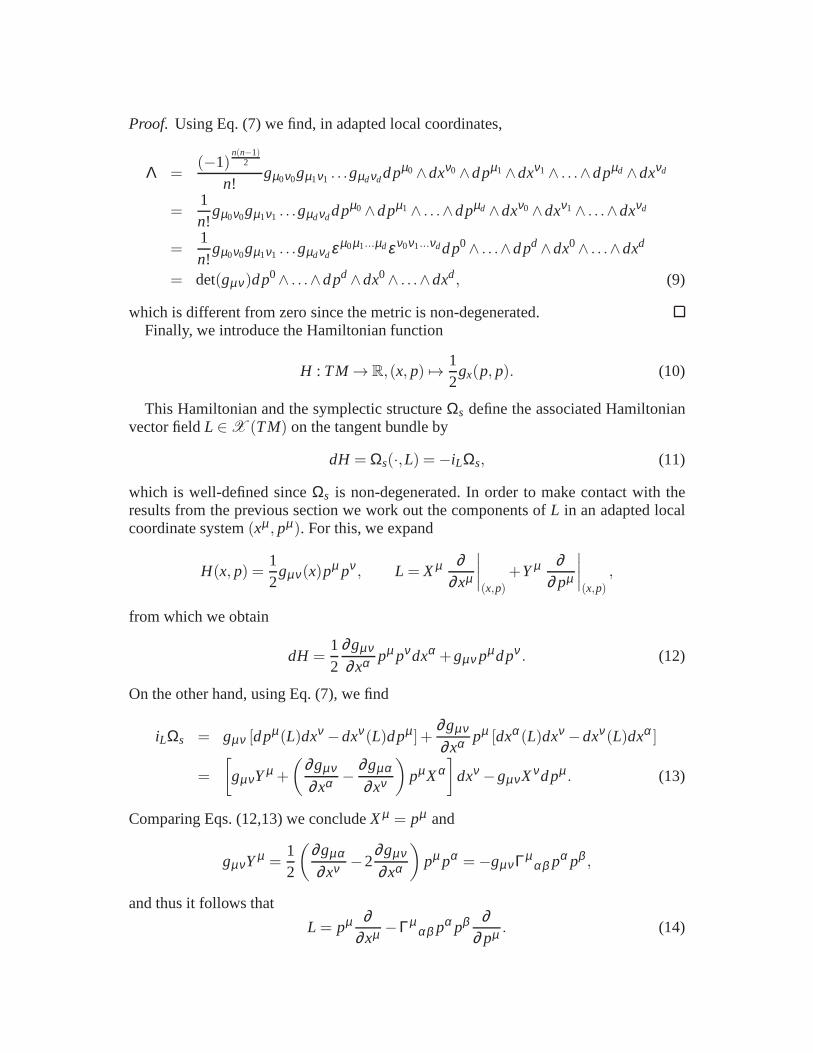
Proof. Using Eq. (7) we find, in adapted local coordinates,

Λ =(−1)

n(n−1)2

n!gµ0ν0gµ1ν1 . . .gµdνddpµ0 ∧dxν0 ∧dpµ1 ∧dxν1 ∧ . . .∧dpµd ∧dxνd

=1n!

gµ0ν0gµ1ν1 . . .gµdνddpµ0 ∧dpµ1 ∧ . . .∧dpµd ∧dxν0 ∧dxν1 ∧ . . .∧dxνd

=1n!

gµ0ν0gµ1ν1 . . .gµdνdεµ0µ1...µdεν0ν1...νddp0∧ . . .∧dpd ∧dx0∧ . . .∧dxd

= det(gµν)dp0∧ . . .∧dpd ∧dx0∧ . . .∧dxd, (9)

which is different from zero since the metric is non-degenerated.Finally, we introduce the Hamiltonian function

H : TM → R,(x, p) 7→12

gx(p, p). (10)

This Hamiltonian and the symplectic structureΩs define the associated Hamiltonianvector fieldL ∈ X (TM) on the tangent bundle by

dH = Ωs(·,L) =−iLΩs, (11)

which is well-defined sinceΩs is non-degenerated. In order to make contact with theresults from the previous section we work out the componentsof L in an adapted localcoordinate system(xµ , pµ). For this, we expand

H(x, p) =12

gµν(x)pµ pν , L = Xµ ∂

∂xµ

∣

∣

∣

∣

(x,p)+Yµ ∂

∂ pµ

∣

∣

∣

∣

(x,p),

from which we obtain

dH =12

∂gµν

∂xα pµ pνdxα +gµν pµdpν . (12)

On the other hand, using Eq. (7), we find

iLΩs = gµν [dpµ(L)dxν −dxν(L)dpµ ]+∂gµν

∂xα pµ [dxα(L)dxν −dxν(L)dxα ]

=

[

gµνYµ +

(

∂gµν

∂xα −∂gµα

∂xν

)

pµXα]

dxν −gµνXνdpµ . (13)

Comparing Eqs. (12,13) we concludeXµ = pµ and

gµνYµ =12

(

∂gµα

∂xν −2∂gµν

∂xα

)

pµ pα =−gµν Γµαβ pα pβ ,

and thus it follows that

L = pµ ∂∂xµ −Γµ

αβ pα pβ ∂∂ pµ . (14)

In the absence of an external electromagnetic field this Hamiltonian vector field co-incides with the Liouville vector field onTM defined in Eq. (3). Therefore, we haveshown:

Theorem 1. Let γ be an integral curve of the Hamiltonian vector field L defined inEq. (11), and consider its projectionγ := π γ onto M. Then,γ is necessarily an affinelyparametrized geodesics: its tangent vector, p satisfies∇pp = 0, with ∇ denoting theLevi-Civita connection belonging to g.

The ideas outlined so far can be extended to diverse physicalsystems. As an example,here we discuss the case of particles with chargeq interacting with an external electro-magnetic and gravitational field. Remarkably, a minimal modification of the Poincaréone-form is sufficient to generalize the previous result. The modified Poincaré one-formis

Θ(x,p)(X) := gx(p,π∗(x,p)(X))+qAx(π∗(x,p)(X)), X ∈ T(x,p)(TM), (15)

whereA∈ Λ1(M) is the electromagnetic potential. In adapted local coordinates Eq. (5)is replaced by

Θ(x,p) =[

gµν(x)pµ +qAν(x)

]

dxν |(x,p) . (16)

This modification is natural in view of the fact that in the presence of an externalelectromagnetic field the canonical momentumΠµ is related to the physical momentumpµ by Πµ = pµ +qAµ . The symplectic formΩs= dΘ now reads

Ωs= gµν(x) dpµ ∧dxν |(x,p)+

[

∂gαν∂xµ (x)pα +

q2

Fµν(x)

]

dxµ ∧dxν |(x,p) , (17)

whereF = dA is the electromagnetic field strength. Note that thisΩs is independent ofthe gauge choice. Furthermore, Eq. (17) shows that the volume formΛ defined in Eq. (8)is unaltered. Choosing the Hamiltonian function as in Eq. (10), the resulting Hamiltonianvector fieldL coincides with the one defined in Eq. (3).

We end this section with a simple but useful result:

Proposition 2. We have £LH = 0, £LΩs = 0 and £LΛ = 0, which implies that thequantities H,Ωs andΛ are invariant with respect to the flow generated by L.

Proof. Using the Cartan identity we first find£LH = iLdH = −i2LΩs = 0 and£LΩs =diLΩs+ iLdΩs = −d2H = 0. With this,£LΛ = 0 follows directly from the definition inEq. (8).

Remark: Since£LΛ = (divΛL)Λ it follows from this proposition that the Liouvillevector field is divergence-free, divΛL = 0. Therefore, relative to the volume formΛ, theflow in TM generated byL is volume-preserving.

THE MASS SHELL

We now consider a simple gas, that is, a collection of neutralor charged, spinlessclassical particles of the same rest massm> 0 and the same chargeq moving in atime-oriented background spacetime(M,g) and an external electromagnetic fieldF. We

assume that the particles interact only via binary elastic collisions idealized as a point-like interaction.4 Therefore, between collisions, for the uncharged case, theparticlesmove along future-directed timelike geodesics of(M,g) while for the charged case theymove along the classical trajectories determined by Eq. (2). From the tangent bundlepoint of view, the gas particles follow segments of integralcurves of the Liouville vectorfield L. Since all gas particles have the same rest mass, these segments are restricted toa particular subsetΓm of TM referred to as the mass shell.Γm is defined as

Γm := H−1(

−m2

2

)

=

(x, p) ∈ TM : 2H(x, p) = gx(p, p) =−m2 , (18)

whereH : TM → R is the Hamiltonian defined in Eq. (10). In this section we discuss afew relevant properties of the mass shell. The first important property is described in thefollowing lemma.

Lemma 2. Γm is a (2n−1)-dimensional C∞-differentiable manifold.

Proof. We consider an arbitrary point(x, p) ∈ Γm. Sincegx(p, p) =−m2 < 0 it followsthat π∗(L) = p 6= 0. Consequently,L(x,p) 6= 0 and it follows fromdH = Ωs(·,L) andthe non-degeneracy ofΩs that dH(x,p) 6= 0. Therefore,Γm is a submanifold ofTM ofco-dimension one, and the lemma follows.

For the proof of the next proposition and the definitions of the current density andstress-energy tensors defined in the next section, the following subset of the tangentspaceTxM at a specific eventx∈ M is useful:

Px := p∈ TxM : gx(p, p) =−m2. (19)

For an arbitrary (not necessarily time-orientable) spacetime (M,g), Px is the union oftwo disjoint setsP+

x and P−x , which may be called the "future" and the "past" mass

hyperboloid atx, respectively. Because the spacetime metric is smooth, this distinctioncan be extended unambiguously to a small neighborhood ofx. However, it can beextended unambiguously to the whole spacetime if and only if(M,g) is time-orientable.

In view of the definition ofPx in Eq. (19) a useful alternative definition ofΓm is

Γm = (x, p) : x∈ M, p∈ Px. (20)

If (M,g) is time-oriented and connected, it follows thatΓm splits into two disjointcomponents which we refer to as "future" and "past". In fact,we have the followingproposition.

Proposition 3. Suppose M is connected and m> 0. Then,(M,g) is time-orientable ifand only ifΓm is disconnected, in which case it is the disjoint union of twoconnectedcomponentsΓ+

m andΓ−m.

4 For the uncharged case, the self-gravity of the gas particles will be incorporated in a self-consistentmanner in the Einstein-Liouville system. For the charged case, the self-gravity and self-electromagneticfield of the gas particles will be taken into account by imposing the Einstein-Maxwell-Vlasov equationsdiscussed further ahead.

Proof. See appendix A.In Lemma 2 we proved thatΓm is a submanifold ofTM. In the next lemma we show

that the volume formΛ on TM defined in Eq. (8) induces a(2n− 1)-form Ω on themass shellΓm which is non-vanishing at every point. In particular,Γm is oriented by thevolume formΩ.

Lemma 3. (i) Consider the open subset V:= (x, p) ∈ TM : H(x, p) < 0 ⊂ TM ofthe tangent bundle. There exists a(2n−1)-formσ on V such that for all(x, p) ∈V

dH(x,p)∧σ(x,p) = Λ(x,p). (21)

(ii) The (2n−1)-formΩ onΓm, defined by the pull-backΩ := ι∗σ of σ with respect tothe inclusion mapι : Γm →V ⊂ TM, is independent of the choice forσ in (i) anddefines a volume form onΓm.

Remark: Notice that the(2n− 1)-form σ is not unique since we can add to it anyfield of the formdH∧β with a (2n−2)-form β . However, the pull-back ofσ to Γm isunique.

Proof. (i) As a first step, we show the existence of a vector fieldN ∈ X (V) withthe property thatdH(N) = 1 onV. For this, consider the one-parameter group ofdiffeomorphismsϕλ :V →V,(x, p) 7→ (x,eλ p), λ ∈R, which induces the rescalingby the factoreλ in each fibre. LetX ∈X (V) be the corresponding generating vectorfield,

X(x,p) :=d

dλϕλ (x, p)

∣

∣

∣

∣

λ=0.

Then, it follows for each(x, p) ∈V that

dH(x,p)(X)=X(x,p)[H] =d

dλH(ϕλ (x, p))

∣

∣

∣

∣

λ=0=

ddλ

12

gx(eλ p,eλ p)

∣

∣

∣

∣

λ=0=2H(x,p).

Therefore,N := X/(2H) yields the desired vector field.Next, defineσ := iNΛ = Λ(N, ·, ·, . . . , ·). We claim that thisσ satisfies Eq. (21).In order to verify this claim, we note that it is sufficient to show that Eq. (21)holds at each(x, p) ∈ V when both sides are evaluated on a particular basis ofT(x,p)(TM). A convenient basis is constructed as follows: consider the(2n− 1)-dimensional submanifoldH = const. through(x, p). SinceN(x,p) is transverse tothis submanifold, it can be completed to a basisX1 := N(x,p),X2, . . . ,X2n ofT(x,p)(TM) such that eachXi , i = 2, . . . ,2n, is tangent to the submanifoldH = const,that is,dH(x,p)(Xi) = 0 for i = 2, . . . ,2n. The claim follows by noting that

dH(x,p)∧σ(x,p)(X1,X2, . . . ,X2n) = σ(x,p)(X2, . . . ,X2n) = Λ(x,p)(N(x,p),X2, . . . ,X2n).

(ii) Let (x, p) ∈ Γm ⊂V and let the basisX1 = N(x,p),X2, . . . ,X2n at (x, p) be definedas above. Then,

Ω(x,p)(X2, . . . ,X2n) = (ι∗σ)(x,p)(X2, . . . ,X2n) = σ(x,p)(X2, . . . ,X2n)

= Λ(x,p)(X1,X2, . . . ,X2n),

where we have used Eq. (21) in the last step. This shows thatΩ(x,p) is uniquelydetermined byΛ(x,p). Furthermore, as a consequence of Proposition 1, the right-hand side is different from zero which proves thatΩ(x,p) 6= 0.

For the formulation of the next result, it is important to note that the Liouvillevector fieldL ∈ X (TM) is tangent toΓm. This property follows from the fact thatdH(L) = iLdH = £LH = 0, see Proposition 2. Therefore, we may also regardL as avector field onΓm.

Theorem 2 (Liouville’s theorem). The volume formΩ on Γm defined in the previouslemma satisfies

£LΩ = (divΩL)Ω = 0. (22)

Proof. Let σ ∈ Λ2n−1(V) be as in Lemma 3(i). Taking the Lie-derivative with respect toL on both sides of Eq. (21) we obtain, taking into account the results from Proposition 2,

dH(x,p)∧ (£Lσ)(x,p) = 0 (23)

for all (x, p) ∈ Γm. Let X2,X3, . . . ,X2n be vector fields onΓm, and letN ∈X (V) be suchthatdH(N) = 1. Evaluating both sides of Eq. (23) on(N,X2,X3, . . . ,X2n), we obtain

0 = (£Lσ)(X2,X3, . . . ,X2n)

= L [σ(X2,X3, . . . ,X2n)]−σ([L,X2],X3, . . . ,X2n)− . . .−σ(X2,X3, . . . , [L,X2n])

= L [Ω(X2,X3, . . . ,X2n)]−Ω([L,X2],X3, . . . ,X2n)− . . .−Ω(X2,X3, . . . , [L,X2n])

= (£LΩ)(X2,X3, . . . ,X2n),

where we have used the properties of the Lie derivative in thesecond and fourth stepand the definition ofΩ plus the fact thatL is tangent toΓm in the third step. Therefore,£LΩ = 0 and the lemma follows.

We close this section by introducing local coordinate charts on the mass shellΓm.For that, let(U,φ) be a local chart of(M,g) with corresponding local coordinates(x0,x1, . . . ,xd), such that

∂∂x0

∣

∣

∣

∣

x,

∂∂x1

∣

∣

∣

∣

x, . . . ,

∂∂xd

∣

∣

∣

∣

x

, x∈U,

is a basis ofTxM, with the property that for eachx∈U , ∂∂x0

∣

∣

∣

xis timelike and ∂

∂xi

∣

∣

∣

x, i =

1,2, . . . ,d are spacelike. Let(V,ψ) denote the local chart ofTM with the correspondingadapted local coordinates(xµ , pµ) constructed in the proof of Lemma 1. Relative tothese local coordinates, the mass shell is determined by

−m2 = gµν(x)pµ pν = g00(x)(p

0)2+2g0 j(x)p0p j +gi j (x)p

i p j . (24)

Therefore, the mass shellΓm can be locally represented as those(xµ , p0, pi) ∈ ψ(V) ⊂R

2n for which p0 = p0±(x

µ , pi) with

p0±(x

µ , pi) :=g0 j(x)p j ±

√

[g0 j(x)p j ]2+[−g00(x)][

m2+gi j (x)pi p j]

−g00(x). (25)

Sinceg00(x) < 0 andgi j (x)pi p j ≥ 0 for all x∈ U , it follows that p0+(x

µ , pi) is positiveandp0

−(xµ , pi) negative. This liberty in the choice ofp0 expresses the fact that locally,

Γm has two disconnected components, representing "future" and "past". If(M,g) is time-orientable, this distinction can be made globally, and in this casep0

±(xµ , pi) parametrize

locally the two disconnected componentsΓ±m of the mass shell, see Proposition 3.

In terms of the local coordinates(xµ , pi) of Γm, we can evaluate the volume formΩ = ι∗(iNΛ) defined in Lemma 3. For that we note that by virtue of Eq. (12) for each(x, p) ∈ Γm∩V the tangent vector

N(x,p) :=1

p±0(xµ , pi)

∂∂ p0

∣

∣

∣

∣

(x,p),

with

p±0(xµ , pi) := g00(x)p

0±(x

µ , pi)+g0 j(x)pj

= ∓√

[g0 j(x)p j ]2+[−g00(x)][

m2+gi j (x)pi p j]

, (26)

satisfiesdH(N) = 1. Therefore, we find for all(x, p) ∈ Γm∩V,

Ω(x,p) = ι∗(iNΛ)(x,p) =det(gµν(x))

p±0(xµ , pi)dp1∧ . . .∧dpd ∧dx0∧dx1∧ . . .∧dxd, (27)

where in the last step we have used the coordinate expressionin Eq. (9).

INTEGRATION OVER THE MASS SHELL

In the previous section we have introduced the mass shellΓm and the volume formΩ on Γm. This volume form is induced from the volume formΛ on the tangent bundleTM, which, in turn is constructed from the Poincaré one-form. From now on, we assume(M,g) to be time-oriented, such that the mass shell splits into twocomponentsΓ±

m, seePropositon 3. In the following, we restrict ourselves to the"future" componentΓ+

m, achoice which incorporates the idea that gas particles move in the future direction.

In this section we first discuss the integral of functions defined on the mass shellΓ+m.

However, for the purpose of the interpretation of kinetic theory, it is also essential tointroduce the integral of real-valued functions defined on 2d-dimensional submanifoldsof Γ+

m.Since onΓ+

m is defined the volume formΩ, the integral of any real-valuedC∞-functions f : Γ+

m → R of compact support is∫

Γ+m

f Ω.

For the purpose of the following analysis, we consider the particular subsets ofΓ+m which

are of the formV := (x, p) : x∈ K, p∈ P+

x , (28)

with K ⊂ M a compact subset ofM which we assume to be contained inside a local chart(U,φ) of M. Relative to such a local chart and the induced local coordinates(xµ , pi) ofΓ+

m introduced in the previous section, the integral of aC∞-function f : Γ+m → R of

compact support overV takes the form

∫

V

f Ω =∫

φ(K)

∫

Rd

f (x, p)det(gµν(x))

p+0(xµ , pi)ddpdnx

=∫

φ(K)

∫

Rd

f (x, p)

√

−det(gµν(x))

−p+0(xµ , pi)ddp

√

−det(gµν(x))dnx (29)

where in these expressions,

x := φ−1(xµ), p := p0+(x

µ , pi)∂

∂x0

∣

∣

∣

∣

x+ p j ∂

∂x j

∣

∣

∣

∣

x. (30)

Provided(M,g) is oriented, the integral overp can be interpreted as a fibre integraloverP+

x . This follows from the observation thatP+x is a submanifold ofTxM, and this

linear space carries the natural volume formηx =√

−det(gµν(x))dx0∧dx1∧ . . .∧dxd.Proceeding as in Lemma 3, the volume formηx induces a volume formπx on P+

x . Interms of coordinates(p0, p j) of TxM chosen such that∂∂ p0 is timelike, ∂

∂ p j are spacelike

for j = 1, . . . ,d, and such thatp0 > 0 onP+x , πx takes the form

πx =

√

−det(gµν(x))

|p+0(xµ , pi)|dp1∧ . . .∧dpd, (31)

with the functionp+0(xµ , pi) given in Eq. (26). In particular, if the coordinates(p0, p j)are chosen such that they determine an inertial frame inTxM, then we havegµν(x) =ηµν , and it follows that

πx =dp1∧ . . .∧dpd√

m2+δi j pi p j,

from which we recognize the special-relativistic Lorentz-invariant volume-form on thefuture mass hyperboloid.

With the definition in Eq. (31) we can rewrite the integral over p in Eq. (29) as a fibreintegral overP+

x , and thus

∫

V

f Ω =

∫

φ(K)

∫

P+x

f (x, p)πx

√

−det(gµν(x))dnx=

∫

K

∫

P+x

f (x, p)πx

η, (32)

where we have used again the fact that(M,g) is oriented and the definition of the naturalvolume formη. We summarize this important result in the following lemma.

Lemma 4 (Local splitting I). Suppose(M,g) is oriented and time-oriented. Let V⊂ Γ+m

be a subset of the future mass shell which is of the form given in Eq. (28), where K⊂ Mis a compact subset of M, contained in a coordinate neighborhood. Suppose f: Γ+

m →R

is C∞-differentiable and has compact support. Then,

∫

V

f Ω =

∫

K

∫

P+x

f (x, p)πx

η, (33)

whereπx is the fibre volume element defined in Eq. (31) andη is the natural volumeelement of(M,g).

We now consider the integration of functionsf : Γ+m → R on suitable submanifoldsΣ

of Γ+m. The submanifolds we are considering are 2d-dimensional and oriented. In order

to define the integral off on Σ we also need a 2d-form. Given the volume formΩ andthe Liouville vector fieldL on Γm a natural definition for such a 2d-form is

ω := iLΩ ∈ Λ2d(Γm). (34)

Denoting byι : Σ → Γ+m the inclusion map, it follows that for eachC∞-function f : Γ+

m →R with compact support the integral

∫

Σ

ι∗( f ω), (35)

is well-defined. Note that for the particular case thatL is transverse toΣ at every pointof Σ, it follows that the pull-back ofω = iLΩ is nowhere vanishing so that it defines avolume form onΣ, and in this caseΣ is automatically oriented. We will come back tothis case at the end of this section.

Relative to the local coordinates(xµ , pi) of Γ+m introduced in the previous section, we

find

ω =det(gµν(x))

p+0(xµ , pi)

1(n−1)!

pµεµν1...νddxν1 ∧ . . .∧dxνd ∧dp1∧ . . .∧dpd

+1

(d−1)!

[

qFiν(x)p

ν −Γiαβ (x)p

α pβ]

εi j2... jddpj2 ∧ . . .∧dpjd ∧dx0∧ . . .∧dxd

.

where we have used Eqs. (3) and (27). In terms of the quantities

ηµ :=1

(n−1)!

√

−det(gµν(x))εµν1...νddxν1 ∧ . . .∧dxνd ,

πi :=1

(d−1)!

√

−det(gµν(x))

|p+0(xµ ,xi)|εi j2... jddpj2 ∧ . . .∧dpjd .

we can rewrite the right-hand side in more compact form,

ω = pµηµ ∧π +[

qFiν(x)p

ν −Γiαβ (x)p

α pβ]

πi ∧η. (36)

For the particular case of hypersurfacesΣ of the form

Σ := (x, p) : x∈ S, p∈ P+x , (37)

with S⊂ M a d-dimensional, spacelike hypersurface inM which is contained inU ,5 wehave

∫

Σ

ι∗( f ω) =

∫

S

∫

P+x

f (x, p)pµ πx

ι∗ηµ , (38)

where ι : S→ M is the inclusion map ofS in M. As a preparation of what followsit is worth noticing that the fibre integral yields a well-defined vector fieldJ on thebase manifold(M,g), see Eq. (39) below. Observing thatJµηµ = iJη we arrive at thefollowing lemma.

Lemma 5 (Local splitting II). Suppose(M,g) is oriented and time-oriented. LetΣ ⊂ Γ+m

be a2d-dimensional submanifold of the mass shell which is of the form given in Eq. (37),where S⊂M is a d-dimensional, spacelike hypersurface of M, contained in a coordinateneighborhood. Suppose f: Γ+

m →R is C∞-differentiable and has compact support. Then,∫

Σ

ι∗( f ω) =∫

S

ι∗(iJη), Jµ :=∫

P+x

f (x, p)pµπx, (39)

whereπx is the fibre volume element defined in Eq. (31) andη is the natural volumeelement of(M,g).

So far, we have assumed the functionf to beC∞-smooth and have compact supporton Γ+

m. Although convenient from a mathematical point of view since the requirementof compact support avoids convergence problems, for the physical interpretation givenin the next section this assumption onf might be too strong. In the following we givea brief explanation of what we believe is the correct function space forf within thecontext of kinetic theory.

For this, we assume spacetime(M,g) to be globally hyperbolic, so that it can befoliated by spacelike Cauchy surfacesSt , t ∈R. There is a corresponding foliation of thefuture mass shellΓ+

m given by

Σt := (x, p) : x∈ St , p∈ P+x , t ∈ R. (40)

SinceSt is spacelike,L is everywhere transverse toΣt , and as discussed above it followsthat the pull-back ofω = iLΩ to Σt defines a volume form onΣt . Therefore, we candefine for each real-valued,C∞-function f : Σt → R of compact support the integral

∫

Σt

f ι∗ω. (41)

5 Notice thatL is transverse toΣ at each point ofΣ sinceS is spacelike. Therefore,Σ is oriented.

In fact, the integral is also well-defined for continuous functions f : Σt →R with compactsupport. In this case, it follows from the Riesz representation theorem (see, for instancechapter 7 in Ref. [25]) that there exists a unique measureµΣt on the space of Borel setsof Σt such that

∫

Σt

f dµΣt =

∫

Σt

f ι∗ω

for all such f . With this measure at hand, one can immediately define the spaceL1(Σt ,dµΣt ). We claim that this is the appropriate function space for kinetic theory.Primary, it turns out that the spaceL1(Σt ,dµΣt ) is, in some sense, independent of theCauchy surfaceSt . The precise statement is contained in the next lemma, whoseproofis sketched in Appendix B.

Proposition 4. Let Σ1 andΣ2 be2d-dimensional submanifolds ofΓ+m with the property

that each integral curve of L intersectsΣ1 andΣ2 exactly at one point. Then, there existsa diffeomorphismϕ : Σ1 → Σ2 such that

∫

Σ2

f dµΣ2 =

∫

Σ1

(ϕ∗ f )dµΣ1

for all C∞-functions f: Σ2 → R of compact support.

Secondly, the physical interpretation that the total number of particles in the gas isfinite is accommodated in our assumption that the integral off overΣt is finite, as wewill see below.

After these remarks concerning the integration of real-valued functions on the massshell we are now ready to discuss physical applications of the above mathematicalformalism.

DISTRIBUTION FUNCTION AND LIOUVILLE EQUATION

As we have mentioned earlier on, for a simple gas, the world lines of the gas particlesbetween collisions are described by integral curves of the Liouville vector fieldL on themass shellΓm. This section is devoted to the definition and properties of the one-particledistribution function and its associated physical observables.

Following Ehlers [24] we consider a Gibbs ensemble of the gason a fixed spacetime(M,g). The central assumption of relativistic kinetic theory is that the averaged prop-erties of the gas are described by a one-particle distribution function. This function isdefined as a nonnegative functionf : Γ+

m → R on the future mass shell such that for any(2d)-dimensional, oriented hypersurfaceΣ ⊂ Γ+

m, the quantity

N[Σ] :=∫

Σ

ι∗( f ω), (42)

gives the ensemble average of occupied trajectories that pass throughΣ. In particular,if Σ = ∂V is the boundary of an open setV ⊂ Γ+

m in Γ+m with (piecewise) smooth

boundaries, then the quantity

N[∂V] =∫

∂V

ι∗( f ω) (43)

gives the ensemble average of the net change in number of occupied trajectories due tocollisions inV.

As explained at the end of the last section, the distributionfunction f lies in the spaceof integrable functionsL1(Σ,dµΣ) with respect to a hypersurfaceΣ of Γ+

m to whichL istransverse. However, for mathematical convenience, we assume in the following thatf isC∞-smooth and is compactly supported on the future mass shellΓ+

m. This automaticallyguarantees the existence of all the integrals we write below.

As a consequence of the interpretation of the integrals (42,43), we show in this sectionthat for a collisionless gas the distribution functionf must obey theLiouville equation

£L f = 0. (44)

The derivation of the Liouville equation (44) is based on thefollowing result.

Proposition 5. The 2d-form ω = iLΩ is closed. Morevover, for any real-valued C∞-function f onΓm we have

d( f ω) = (£L f )Ω. (45)

Proof. The proposition is a consequence of Liouville’s theorem (Theorem 2) and theCartan identity. Using these results one finds

(£L f )Ω = £L( f Ω) = (diL+ iLd)( f Ω) = d( f iLΩ) = d( f ω).

In particular, for f = 1 it follows thatdω = 0.By means of Stokes’ theorem and this proposition we can rewrite the integral in

Eq. (43) as

N[∂V] =∫

V

d( f ω) =∫

V

(£L f )Ω. (46)

In particular, letV =⋃

0≤t≤T Σt be the tubular region obtained by letting flow a(2d)-dimensional hypersurfaceΣ0 in Γ+

m to which L is transverse along the integral curvesof L. Since by definitionL is tangent to the cylindrical piece,T :=

⋃

0≤t≤T ∂Σt , of theboundary, it follows that

∫

Tf ω = 0. Therefore, we obtain from Eqs. (42,46)

N[ΣT ]−N[Σ0] =∫

V

(£L f )Ω,

that is, the averaged number of occupied trajectories atΣT is equal to the averagednumber of occupied trajectories atΣ0 plus the change in occupation number due tocollisions in the regionV. For a collisionless gas the integral in Eq. (46) must be zerofor all volumesV, and in this case the distribution functionf must satisfy the Liouvilleequation

£L f = 0. (47)

Using Eq. (3) we find

(£L f )(x, p) = pµ ∂ f∂xµ (x, p)+

[

qFµν(x)p

ν −Γµαβ (x)p

α pβ] ∂ f

∂ pµ (x, p) = 0 (48)

in adapted local coordinates ofTM. The above Liouville equation can also be rewrittenas an equation for the functionf (xµ , pi) := f (x, p), depending on the local coordinates(xµ , pi) of the future mass shellΓ+

m introduced earlier, where we recall the definitions ofx and p in Eq. (30). By differentiating both sides of Eq. (24) one finds

∂ p0+(x

µ , p j)

∂xµ =−1

2p+0(xµ , p j)pα pβ ∂gαβ

∂xµ ,∂ p0

+(xµ , p j)

∂ pi =−1

p+0(xµ , p j)giβ pβ ,

where here ˆp0 = p0+(x

µ , p j) and p j = p j . Using this and

∂ f∂xµ =

∂ f∂xµ +

∂ f∂ p0

∂ p0+

∂xµ =∂ f∂xµ −

pα pβ

2p+0

∂gαβ

∂xµ∂ f∂ p0 ,

∂ f∂ pi =

∂ f∂ pi +

∂ f∂ p0

∂ p0+

∂ pi =∂ f∂ pi −

giβ pβ

p+0

∂ f∂ p0 ,

Eq. (48) can be rewritten in terms of the local coordinates(xµ , p j) on the mass shell as

pν ∂ f∂xν (x

µ , p j)+[

qFiν(x)p

ν −Γiαβ (x)p

α pβ] ∂ f

∂ pi (xµ , p j) = 0. (49)

CURRENT DENSITY AND STRESS-ENERGY TENSOR

In this section, using the distribution functionf , we construct important tensor fieldson the spacetime manifold(M,g) by integrating suitable geometric quantities involvingf over the future mass hyperboloidalP+

x . At this point, we remind the reader that(M,g)is assumed to be oriented and time-oriented, and thusP+

x carries the natural volume formπx defined in Eq. (31).

We restrict our consideration to the quantities defined by:

Jx(α) :=∫

P+x

f (x, p)α(p)πx (current density), (50)

Tx(α,β ) :=∫

P+x

f (x, p)α(p)β (p)πx (stress-energy tensor), (51)

where hereα,β ∈ T∗x M. Since f : Γ+

m → R is assumed to be smooth and compactlysupported, these quantities are well-defined. Moreover, byconstruction,Jx is linear inαandTx bilinear in (α,β ), and thusJ andT define a vector field and a symmetric, con-travariant tensor field onM, respectively. Their components relative to local coordinates

(xµ) of M are obtained fromJµ(x) = Jx(dxµ), Tµν(x) = Tx(dxµ ,dxν), which yields

Jµ(x) =∫

P+x

f (x, p)pµπx =∫

Rd

f (x, p)pµ

|p0+(xµ , pi)|

√

−det(gµν(x))ddp, (52)

Tµν(x) =

∫

P+x

f (x, p)pµ pν πx =

∫

Rd

f (x, p)pµ pν

|p0+(xµ , pi)|

√

−det(gµν(x))ddp, (53)

where here(xµ , pi) are the adapted local coordinates ofΓ+m with the functionp0+(xµ , pi)

defined in Eq. (26). It follows from these expressions thatJ andT areC∞-smooth tensorfields onM.

The physical significance of these tensor fields can be understood by consideringa future-directed observer in(M,g) whose four-velocity isu. At any eventx alongthe observer’s world line, we choose an orthonormal frame sothat gµν(x) = ηµν anduµ = δ µ

0 . Relative to this rest frame we have the usual relations fromspecial relativity,

(pµ) = (E, pi) = mγ(1,vi), γ =1

√

1−δi j viv j,

with vi the three-velocity of a gas particle measured by the observer at x. Therefore, inthe observer’s rest frame, we have the following expressions which are familiar from thenon-relativistic kinetic theory of gases:

J0(x) =∫

Rd

f (x, p)ddp= n(x), (particle density) (54)

Ji(x) =

∫

Rd

f (x, p)viddp= n(x)< vi >x, (particle current density) (55)

T00(x) =∫

Rd

f (x, p)Eddp= n(x)< E >x, (energy density) (56)

T0 j(x) =∫

Rd

f (x, p)p jddp= n(x)< p j >x, (momentum density) (57)

T i j (x) =

∫

Rd

f (x, p)vi p jddp= n(x)< vi p j >x, (kinetic pressure tensor),(58)

where the average< A>x at x∈ M of a functionA : Γm → R on phase space is definedas

< A>x:=

∫

Rd

A(x, p) f (x, p)ddp

∫

Rd

f (x, p)ddp=

1n(x)

∫

Rd

A(x, p) f (x, p)ddp.

We also define the mean kinetic pressure by

p(x) :=1d

T ii(x) =

1d

n(x)< vi pi >x,

and writeρ(x) := mn(x) for the rest mass density. We stress that these quantities areobserver-dependent; so far, only the tensor fieldsJ andT defined in Eqs. (50,51) have acovariant meaning. It is worth noting the following Lemma (cf. Eq. (111) in Ref. [24])

Lemma 6. The (observer-dependent) quantitiesε(x) := n(x) < E >x, p(x) and ρ(x)satisfy the following inequalities:

0≤ dp(x)≤d2

p(x)+

√

[

d2

p(x)

]2

+ρ(x)2 ≤ ε(x)≤ ρ(x)+dp(x). (59)

for all x ∈ M.

Proof. The first two inequalities are obvious sincep ≥ 0. For the last two inequalities,we first observe that

ε(x)−dp(x) = m∫

Rd

γ−1 f (x, p)ddp.

Since γ−1 ≤ 1 the fourth inequality follows immediately. Next, using the Cauchy-Schwarz inequality:

ρ(x)2 = m2

∫

Rd

γ1/2γ−1/2 f (x, p)ddp

2

≤

∫

Rd

mγ f (x, p)ddp∫

Rd

mγ−1 f (x, p)ddp= ε(x) [ε(x)−dp(x)] ,

from which the third inequality follows.After these estimates concerning observer-dependent quantities, we now turn to co-

variant considerations. For this, the following lemma is useful (cf. [26]):

Lemma 7. Consider a vector p and a covariant, symmetric tensor T on a finite-dimensional vector space V with Lorentz metric g. Then, the following statements hold:

(i) p ∈ V is future-directed timelike if and only if g(p,k) < 0 for all non-vanishing,future-directed causal vectors k∈V.

(ii) Suppose that T(k,k)> 0 for all non-vanishing null vectors k∈V. Then, there existsa timelike vector k∗ such that

T(k∗, ·) =−λg(k∗, ·)

with λ ∈R. If, in addition T(k,k)≥ 0 for all vectors k∈V, then the timelike vectork∗ is unique up to a rescaling.

Proof. See Appendix C.Using this lemma, we establish that at any given eventx ∈ M with f (x, ·) not iden-

tically zero, the current densityJx and the stress-energy tensorTx satisfy the follow-ing properties: By appealing to statement (i) of this Lemma and the definition ofJx

in Eq. (50) we conclude thatgx(Jx,k) < 0 for all non-vanishing, future-directed causalvectorsk∈ TxM. Therefore, using again Lemma 7(i), it follows thatJx is future-directedtimelike. Likewise, the definition ofTx in Eq. (51) and Lemma 7(i) imply thatTx(k,k)≥ 0for all covectorsk∈ T∗

x M, with strict inequality ifk is non-vanishing causal. Therefore,by Lemma 7(ii), the linear mapTx : TxM → TxM associated toTx has a unique timelikeeigenvectork∈ P+

x ,Tx(k) =−λk. (60)

As a consequence, the stress-energy tensor admits the unique decomposition

Tx = λu⊗u+π , g(u,u) =−1, π(u, ·) = 0, (61)

whereu := k/m. Physical observers moving with this four-velocityu measure densityε(x) = λ , vanishing momentum density, and stresses described byπ . For this rea-son,u is referred to as thedynamical mean velocityof the gas. The stress tensorπis orthogonal tou and symmetric; therefore, it is diagonalizable. We call theeigen-valuesp1(x), p2(x), . . . , pd(x) the principal pressures. It follows from Tx(k,k) ≥ 0 andtrace(Tx) < 0 thatp j(x) ≥ 0 for all j = 1,2, . . . ,d and thatε(x) > p1(x)+ p2(x)+ . . .+pd(x)≥ 0, which implies thatTx satisfies the weak, the strong, and the dominant energyconditions, see Section 9.2 in Ref. [27].

After having introduced the current density and the stress-energy tensor, definedas the first- and second momenta of the distribution functionover the fibre, we askourselves whether or not they satisfy the required conservation laws, provided theLiouville equation (47) holds. The answer is in the affirmative:

Proposition 6. Let f : Γ+m →R be a C∞-function of compact support on the future mass

shell. Then, the following identities hold for all x∈ M:

divJx =∫

P+x

£L f (x, p)πx, (62)

divTx(β ) =∫

P+x

(£L f (x, p))β (p)πx+qβ (Fx(J)), (63)

for all β ∈T∗x M, where L is the Liouville vector field defined in Eq. (3), andF : X (M)→

X (M) was defined just after Eq. (2).

Proof. Choose a local chart(U,φ) of M and letK ⊂ U be a compact, oriented subsetwith C∞-boundary∂K in M. Consider the subset

V := (x, p) : x∈ K, p∈ P+x ⊂ Γ+

m,

cf. Eq. (28), whose boundary is given by the 2d-dimensional, oriented submanifold

∂V = (x, p) : x∈ ∂K, p∈ P+x

of Γ+m. We compute the averaged number of collisions insideV in two different ways.

First, using Eq. (46) and the local splitting result in Lemma4, we have

N(∂V) =

∫

V

(£L f )Ω =

∫

K

∫

P+x

£L f (x, p)πx

η. (64)

On the other hand, using the definition ofN(∂V), the local splitting result in Lemma 5,Stokes’ theorem and Cartan’s identity, we find

N(∂V) =

∫

∂V

f ω =

∫

∂K

iJη =

∫

K

diJη =

∫

K

£Jη =

∫

K

(divJ)η. (65)

Comparing Eqs. (64,65), and taking into account thatK can be chosen arbitrarily small,yields the first claim, Eq. (62) of the lemma.

For the second identity, we fix a one-formβ on M, and replace the four-currentdensityJ by J := T(·,β ) in Eq. (62), which is equivalent to formally replacef (x, p)by f (x, p)β (p) in the calculation above. Then, we obtain

div Jx =∫

P+x

£L [ f (x, p)β (p)]πx =∫

P+x

(£L f (x, p))β (p)πx+∫

P+x

f (x, p) [£L(β (p))]πx.

Using local coordinates, we find on one hand divJ = ∇µ(Tµνβν) = (divT)(β ) +Tµν∇µβν , and on the other hand

£L(β (p)) = L[βµ(x)pµ ] = pµ pν ∇µβν +qFµ

ν(x)pνβµ ,

where we have used the coordinate expression (3) for the Liouville vector fieldL. Theseobservations, together with the definitions in Eqs. (52,53)of Jµ and Tµν yield thedesired result.

THE EINSTEIN-MAXWELL-VLASOV SYSTEM

In this section we consider a simple gas of charged particlesand take into accountits self-gravitation and the self-electromagnetic field generated by the charges. Thissystem is described by an oriented and time-oriented spacetime manifold(M,g) withg the gravitational field, an electromagnetic field tensorF, and a distribution functionf : Γ+

m → R describing the state of the gas. These fields obey the Einstein-Maxwell-Vlasov equations, given by

Gµν = 8πGN

(

Temµν +Tgas

µν

)

, (66)

∇νFµν = qJµ , ∇[µFαβ ] = 0, (67)£L f = 0, (68)

whereG denotes the Einstein tensor,GN Newton’s constant, and where

Temµν = FµαFν

α −14

gµνFαβ Fαβ (69)

is the stress-energy tensor associated to the electromagnetic field,

Tgasµν =

∫

P+x

f (x, p)pµ pν πx (70)

the stress-energy tensor associated to the gas particles, and

Jµ =

∫

P+x

f (x, p)pµ πx (71)

is the particles’ current density. Notice that thetotal stress-energy tensor is divergence-free, as a consequence of the identity (63), Maxwell’s equations (67), and the Vlasovequation (68). Similarly, the divergence-free character of the current density followsfrom the identity (63) and Eq. (68). For recent work related to the above system, seeRefs. [28, 29, 30].

THE RELATIVISTIC BOLTZMANN EQUATION FOR A SIMPLEGAS

In the previous sections we developed the theory describinga collisionless simplegas. For the development of this theory, we postulated that the averaged properties ofthe gas are described by a one-particle distribution function f defined on the future massshell Γ+

m and by simple arguments concluded that this distribution function obeys theLiouville equation£L f = 0.

However, undoubtedly one of the most important equations inthe kinetic theory ofgases is the famous Boltzmann equation, and in order to complete this work, in thissection we shall sketch the structure of this equation. Likethe Liouville equation, thecentral ingredient of the Boltzmann equation is again the one-particle distribution func-tion f associated to the gas. However, and in sharp contrast to the previous equations, theBoltzmann equation describes the time evolution of a systemwhere collisions betweenthe gas particles can no longer be neglected. This occurs when the mean free path (meanfree time) is much shorter than the characteristic length scale (time) associated with thesystem.

In order to describe the Boltzmann equation, for simplicitywe consider a simplecharged gas i.e. a collection of spinless, classical particles which are all of the same restmassm> 0 and all have the same chargeq, and which interact only via binary elasticcollisions. For the purpose of this section we shall neglectthe self-gravity and the self-electromagnetic field of the gas, assuming a fixed backgroundspacetime(M,g) which isoriented and time-oriented. For the uncharged case, the gasparticles move along future-directed timelike geodesics of(M,g) except at binary collisions which are idealized as

point-like interactions. If at an eventx∈ M a binary collision occurs, then two geodesicsegments representing the trajectories of the gas particles end and two new ones emerge.The nature and properties of the emerging geodesics are described by probabilistic lawsincorporated in the transition probability through a Lorentz scalar which is the basicingredient of the collision integral. The history of the gasin the spacetime consists of acollection of broken future-directed geodesic segments describing the particles betweencollisions. In the charged case, the same situation occurs except that the geodesicsegments are replaced by segments of the classical trajectories of Eq. (2).

If p1, p2 stand for the four-momenta of the incoming particles andp3, p4 for themomenta of the outgoing particles at the eventx, then an elastic collision obeys thelocal conservation law:

p1+ p2 = p3+ p4. (72)

In the tangent bundle description such a binary collision atx ∈ M involves four points(x, p1),(x, p2),(x, p3),(x, p4) belonging to the same mass shellΓ+

m and additionally fourorbits of the Liouville vector fieldL. In particular, the orbits through(x, p1),(x, p2)become unoccupied while the orbits through(x, p3),(x, p4) become occupied. Thisinterchange in the occupation of the orbits ofL is the effect of a binary collision asperceived from the mass shellΓ+

m.Like for the case of a collisionless system, it is postulatedthat its averaged properties

are described by a distribution functionf : Γ+m → R on the mass shellΓ+

m, defined byEq. (42). However, the Liouville equation is replaced by theBoltzmann equation whichhas the following form:

£L f (x, p) =∫

P+x

∫

P+x

∫

P+x

W(p3+ p4 7→ p+ p2)

× [ f (x, p4) f (x, p3)− f (x, p) f (x, p2]πx(p4)πx(p3)πx(p2), (73)

where the right-hand side is the collision integral describing the effects of binary col-lisions. The quantityW(p3+ p4 7→ p+ p2) is referred to as the transition probabilityscalar, and it obeys the following symmetries:

W(p3+ p4 7→ p+ p2) =W(p4+ p3 7→ p2+ p), (74)W(p+ p2 7→ p3+ p4) =W(p3+ p4 7→ p+ p2). (75)

The first symmetry is trivial, while the second symmetry expresses microscopic re-versibility or, as often called, the principle of detailed balancing [10].

Intuitively speaking the term∫

P+x

∫

P+x

∫

P+x

W(p3+ p4 7→ p+ p2) f (x, p4) f (x, p3)πx(p4)πx(p3)πx(p2)

in the collision integral describes the averaged number of collisions taking place in aninfinitesimal volume element centered aroundx∈ M whose net effect is to increase the

averaged number of occupied orbits through(x, p). On the other hand the term

−∫

P+x

∫

P+x

∫

P+x

W(p3+ p4 7→ p+ p2) f (x, p) f (x, p2)πx(p4)πx(p3)πx(p2)

describes the depletion of the occupied orbits through(x, p) due to the binary scattering.In the previous sections we have shown that the mere existence of the distribution

function f : Γ+m → R leads to the construction of the current densityJ and stress-energy

tensorT describing the gas, and naturally this property off remains valid for a collision-dominated gas. For a collisionless gasJ andT satisfy the conservation laws divJ = 0,divT = qF(J), as a consequence of the Liouville equation£L f = 0, see Proposition 6.We shall show below that these properties ofJ andT remain valid for the case wherethe distribution function satisfies the Boltzmann equation, Eq. (73).

In order to prove this property, letΨ : Γ+m → R : (x, p) 7→ Ψ(x, p) be an arbitraryC∞-

smooth real-valued function. Multiplying both sides of Boltzmann equation byΨ andintegrating overP+

x yields∫

P+x

Ψ(x, p)£L f (x, p)πx(p)

= −14

∫

P+x

∫

P+x

∫

P+x

∫

P+x

W(p3+ p4 7→ p+ p2) [Ψ(x, p4)+Ψ(x, p3)−Ψ(x, p)−Ψ(x, p2)]

× [ f (x, p4) f (x, p3)− f (x, p) f (x, p2]πx(p4)πx(p3)πx(p2)πx(p), (76)

where we have made use of the symmetry properties (74,75) forthe transition probabilityscalar. In particular, the right-hand side vanishes identically if Ψ is chosen to be acollision-invariant quantity. The choiceΨ(x, p) = 1 leads to

∫

P+x

£L f (x, p)πx(p) = 0,

which implies thatJ is divergence-free, see Eq. (62), while the choiceΨ(x, p) = βx(p)from someβ ∈ Λ1(M), together with the momentum conservation law, Eq. (72), yields

∫

P+x

βx(p)£L f (x, p)πx(p) = 0,

which implies that divTx(βx) = qβx(Fx(J)), see Eq. (63).However, by far the most important implication of the Boltzmann equation is the

existence of a vector fieldS on (M,g) whose covariant divergence is semi-positivedefinite provided that micro-reversibility holds. In orderto construct this field, weassume for the following that the distribution function isstrictly positive, with suitablefall-off conditions to guarantee the convergence of the integrals below. Since we abstainfrom specifying such fall-off conditions explicitly, the following arguments should be

taken as formal. We chooseΨ(x, p) = 1+ log(A f(x, p)), whereA has been insertedto make the argument of the logarithm a dimensionless quantity. For this choice, theidentity (76) yields

∫

P+x

[1+ log(A f(x, p))]£L f (x, p)πx(p) =−14

∫

P+x

∫

P+x

∫

P+x

∫

P+x

W(p1+ p2 7→ p3+ p4)

× [log( f1 f2)− log( f3 f4)] [ f1 f2− f3 f4]πx(p1)πx(p2)πx(p3)πx(p4),

where we have abbreviatedf j := f (x, p j) for j = 1,2,3,4. The right-hand side is non-positive, due to the positivity ofW(p1+ p2 7→ p3+ p4) and the inequality

(logy− logx)(y−x)≥ 0,

which is valid for all x,y > 0. On the other hand, noting that[1+ log(A f)]£L f =£L[log(A f) f ] we obtain, by replacing the functionf with the function log(A f) f inEq. (62),

divSx =−

∫

P+x

[1+ log(A f(x, p))]£L f (x, p)πx(p),

with the entropy flux vector fieldSdefined by

Sx(α) :=−∫

P+x

log(A f(x, p)) f (x, p)α(p)πx, (77)

for α ∈ T∗x M. Therefore, the entropy flux vector fieldSsatisfies

divSx =14

∫

P+x

∫

P+x

∫

P+x

∫

P+x

W(p1+ p2 7→ p3+ p4)

× [log( f1 f2)− log( f3 f4)] [ f1 f2− f3 f4]πx(p1)πx(p2)πx(p3)πx(p4)≥ 0.

The above relation expresses the famous Boltzmann H-theorem. It is beyond the scopeof this article to provide a detailed discussion of the mathematical framework underlyingthe structure of the collision integral and related properties of the Boltzmann equation.The reader is referred to Refs. [31, 18, 17] for a more detailed discussion and propertiesof the Boltzmann equation.

CONCLUSIONS

In this work, we have presented a mathematically-oriented introduction to the fieldof relativistic kinetic theory. Our emphasis has been placed on the basic ingredients thatconstitute the foundations of the theory. As it has become clear, of a prime importancefor the description of this theory are not any longer point particles but rather andaccording to Synge’s fundamental idea, world lines of gas particles. From the tangentbundle point of view, these world lines appeared as the integral curves of a Hamiltonian

vector field. It is worth stressing here the liberty and the flexibility that characterizes therelativistic kinetic theory of gases. The Poincaré one-form as well as the Hamiltonianand thus the structure of the Hamiltonian vector field are at our disposal. In this workwe have made simple and natural choices for the Poincaré one-form and Hamiltonian,and we were led from first principles to the Liouville equation, while for the case wherethe self-gravity and self-electromagnetic field of the gas are accounted for we arrivednaturally to the Einstein-Liouville and the Einstein-Maxwell-Vlasov systems.

Therefore, given the freedom in the Poincaré one-form and the Hamiltonian it is worththinking of relativistic kinetic theory models describingdark matter or dark energy. Thiscould be interesting from an astrophysical and cosmological point of view.

ACKNOWLEDGMENTS

This work was supported in part by CONACyT Grant No. 101353 and by a CIC Grantto Universidad Michoacana.

APPENDIX A: PROOF OF PROPOSITION 3

We prove thatΓm is connected if and only if(M,g) is not time-orientable. Supposefirst that Γm is connected and let us show that(M,g) cannot be time-orientable. Forthis, choose an arbitrary pointx ∈ M and two timelike tangent vectorsk+ and k−at x such thatk± ∈ P±

x . Since Γm is connected by hypothesis, there exists a curveγ : [0,1]→ Γm, t 7→ (γ(t),k(t)) which connects the two points(x,k+) and(x,k−). Theprojection of this curve yields a closed curveγ : [0,1]→ M in M throughx. Along thiscurve is defined the continuous timelike vector fieldk(t) which connectsk+ andk− (seeFig. 1). Therefore,(M,g) is not time-orientable.

Conversely, suppose(M,g) is not time-orientable. We shall prove thatΓm is con-nected. In order to show this we note the hypothesis implies the following. There existsan eventx∈ M, a closed curveγ : [0,1]→ M throughx and a continuous timelike vectorfield k(t) ∈ Tγ(t)M alongγ which we may normalize such thatg(k(t),k(t)) = −m2 forall t ∈ [0,1], with the property thatk− := k(0)∈ P−

x andk+ := k(1)∈ P+x . In this way we

obtain a curveγ : [0,1]→ Γm, t 7→ (γ(t),k(t)) in Γm which connects(x,k−) with (x,k+).Since the setsP±

x are connected, it follows that any two points(x, p),(x, p′) ∈ Γm in thesame fibre overx can be connected to each other by a curve inΓm.

Now let us extend this connectedness property to arbitrary points(x1, p1),(x2, p2) ∈Γm. SinceM is connected there exist curvesγ1,γ2 in M which connectx with x1 andxwith x2, respectively. By parallel transportingp1 alongγ1 and p2 alongγ2 we obtaincurves γ1 and γ2 in Γm which connect(x1, p1) with (x, p) and (x2, p2) with (x, p′)respectively.6 By the result in the previous paragraph,(x, p) and(x, p′) can be connectedto each other by a curve inΓm. Therefore,(x1, p1) and(x2, p2) can also be connected toeach other and it follows thatΓm is connected.

6 γ1 andγ2 are the horizontal lifts ofγ1 andγ2 through the points(x1, p1) and(x2, p2), respectively.

M

γk

k+

x1γ1

PxTM

x

k−

(x, k+)

(x, k−)

γ

FIGURE 1. An illustration of the curvesγ ⊂ TM andγ ⊂ M, together with the vector fieldk alongγ.

In order to conclude the proof we need to show thatΓm consists of two connectedcomponents if(M,g) is time-orientable. In order to prove this, choosex∈ M and a time-orientationP+

x andP−x at x. Given any pointy∈ M we may connect it tox by means of

a curveγ in M sinceM is connected. We choose the time orientationP±y at y such that

kx ∈ P+x if and only if ky ∈ P+

y for all parallel transported timelike vector fieldsk alongγ. This choice is independent ofγ otherwise(M,g) would not be time-orientable. In thisway we obtain the two connected subsets

Γ±m := (x, p) ∈ Γm : p∈ P±

x

of Γm which are disjoint and whose union isΓm.

APPENDIX B: SKETCH OF THE PROOF OF PROPOSITION 4

We defineϕ : Σ1 → Σ2 to be the map that associates to each pointp1 ∈ Σ1 the uniquepoint p2 ∈ Σ2 that lies on the integral curve ofL throughp1. By transporting the valuesof f along the integral curve ofL in the segment betweenΣ1 andΣ2, we can extendfto aC∞-function f : Γ+

m → R with compact support, such that£L f = 0 in the regionVbetweenΣ1 andΣ2. It follows by Stokes’ theorem that

∫

Σ2

ι∗2( f ω)−∫

Σ1

ι∗1( f ω) =∫

V

d( f ω) =∫

V

(£L f )Ω = 0,

whereι j : Σ j → Γ+m denote the inclusion maps forj = 1,2, and where we have used

Proposition 5 in the second step. Sinceι∗2 f = f andι∗1 f = ϕ∗ f the Proposition follows.

APPENDIX C: PROOF OF LEMMA 7

Without loss of generality we can assume that(V,g) is Minkowski spacetime, so thatthe standard special relativistic notions of causality hold. We work in coordinates(xµ)for which the metric has the standard diagonal form.

(i) At first we note that any non-vanishing causal, future-directed vectork ∈ V hasthe components(kµ) = (k0,ki) with k0 > 0 andδi j kik j ≤ (k0)2. Suppose first thatp ∈ V is future-directed timelike. Then, after a Lorentz transformation, (pµ) =(p0,0, . . . ,0) with p0 > 0 and it follows thatg(p,k) = −p0k0 < 0. Conversely,suppose thatg(p,k) < 0 for all non-vanishing causal, future-directedk. After arotation the components ofp are (pµ) = (p0, p1,0, . . . ,0) and the two choices(kµ

+) = (1,1,0, . . . ,0) and(kµ−) = (1,−1,0, . . . ,0) lead to 0> g(p,k+) =−p0+ p1

and 0> g(p,k−) =−p0− p1 which implies|p1| < p0, and hence, thatp is future-directed timelike.Remark: In fact, as the proof shows, it is sufficient to requirek to be non-vanishingnull and future-directed in order to show thatp is future-directed timelike.

(ii) Consider the unit mass hyperboloid

H+ := u∈V : g(u,u) =−1,u0 > 0,

whose elements may be parametrized according to the stereographic map,

u0 =1

√

1−|v|2, ui =

vi√

1−|v|2, v∈ B1(0),

with B1(0) := v∈R3 : δi j viv j < 1 the unit open ball centered at the origin. Then,

we have onH+,

T(u,u) =1

1−|v|2[

T00+2T0ivi +Ti j v

iv j]=: f (v),

where the functionf : B1(0)→R is smooth. Supposev→ e, |e|= 1, approaches theboundary of its domain. Then, sinceT00+2T0ivi +Ti j viv j → T(k,k) with the nullvectork = (1,e), and since by assumptionT(k,k) > 0, it follows that f (v) → ∞.Therefore, the functionf has a global minimum at some pointv∗ ∈ B1(0). Takingthe gradient on both sides of7

(1−|v|2) f (v) = T00+2T0ivi +Ti j v

iv j

and evaluating atv= v∗, we obtain

− f (v∗)v∗i = T0i +Ti j (v∗) j ,

7 Alternatively, one might also invoke the Lagrange multiplier method, applied to the restriction of thequadratic formT(u,u) onH+, in order to conclude that at the minimumu∗, T(u∗, ·) =−λg(u∗, ·).

from which we also have− f (v∗)|v∗|2 = T0i(v∗)i + Ti j (v∗)i(v∗) j and so f (v∗) =T00+ T0i(v∗)i . Therefore, the timelike vectork∗ := (1,v∗) satisfiesTµν(k∗)ν =−λk∗µ with λ = f (v∗).As for uniqueness, we first observe that after a rescaling anda Lorentz transfor-mation we may assume thatk∗ = (1,0,0, . . . ,0). Then,T00 = λ , T0 j = 0, and byapplying a rotation if necessary, we can assume thatTi j is diagonal, such that(Tµν) = diag(λ , p1, p2, . . . , pd). It follows from the hypothesis thatλ ≥ 0 andp j ≥0 for all j = 1,2, . . . ,d. Furthermore,λ =0 impliesp j >0 for all j =1,2, . . . ,dbecause of the hypothesis. Therefore, the eigenspace belonging to the eigenvalue−λ of the matrix(Tµ

ν) = diag(−λ , p1, p2, . . . , pd) must be one-dimensional since−λ 6= p j for all j = 1,2, . . . ,d.

Remark: Due to the fact that the scalar product defined by the Lorentzmetric g isnot positive definite, it is not always the case that the stress-energy tensorTµν can bediagonalized, despite of the fact that it is symmetric. In fact, the results above show thatTµν is diagonalizable if and only if it admits a timelike eigenvector. An explicit examplefor which the condition in assumption (ii) in Lemma 7 is not satisfied is

Tµν = kµkν

with a null vectork, corresponding to a stress-energy tensor for null dust. In this case,the only eigenvalue ofTµ

ν is zero, and its eigenspace consists of the vectors which areorthogonal tok. In particular, this example shows that the imposition of the weak energycondition is not sufficient to guarantee the diagonalizability of the stress-energy tensor.

REFERENCES

1. C. Cercignani,Ludwig Boltzmann, The Man Who Trusted Atoms, Oxford University Press, Oxford,2010.

2. F. Jüttner,Annal. Phys.34, 856–882 (1911).3. F. Jüttner,Annal. Phys.35, 145–161 (1911).4. F. Jüttner,Z. Phys.47, 542–566 (1928).5. W. Pauli,Theory of Relativity, Dover Publications, New York, 1981.6. R. Tolman,Relativity, Thermodynamics and Cosmology, Dover Publications, New York, 1987.7. J. Synge,Trans. Royal Soc. Canada28, 127–171 (1934).8. J. Synge,The Relativistic Gas, North-Holland, Amsterdam, 1957.9. G. Tauber, and J. Weinberg,Phys. Rev.122, 1342–1365 (1961).10. W. Israel,J. Math. Phys.4, 1163–1181 (1963).11. W. Israel,Annals of Physics100, 310–331 (1976).12. W. Israel, and J. Stewart,Phys. Lett. A58, 213–215 (1976).13. W. Israel, and J. Stewart,Annals Phys.118, 341–372 (1979).14. W. Israel, and J. Stewart,Proc. R. Soc. Lond. A365, 43–52 (1979).15. W. Hiscock, and L. Lindblom,Annals Phys.151, 466–496 (1983).16. W. Hiscock, and L. Lindblom,Phys. Rev. D31, 752–733 (1985).17. C. Cercignani, and G. Kremer,The Relativistic Boltzmann Equation: Theory and Applications,

Birkhäuser, Basel, 2002.18. D. Bancel, and Y. Choquet-Bruhat,Comm. Math. Phys.33, 83–96 (1973).19. A. Rendall, “The Einstein-Vlasov system,” inThe Einstein equations and the large scale behavior of

gravitational fields, edited by P. Chrusciel, and H. Friedrich, 2004, pp. 231–250.20. G. Rein, and A. Rendall,Comm. Math. Phys.150, 561–583 (1992).

21. N. Noutchegueme, and M. Tetsadjio,Class.Quant.Grav.26, 195001 (2009).22. H. Andréasson,Living Reviews in Relativity14 (2011), URLhttp://www.livingreviews.

org/lrr-2011-4.23. M. Dafermos, and A. Rendall (2007),gr-qc/0701034.24. J. Ehlers, “General relativity and kinetic theory,” inGeneral Relativity and Cosmology, edited by

R. Sachs, 1971, pp. 1–70.25. R. Abraham, J. Marsden, and T. Ratiu,Manifolds, Tensor Analysis, and Applications, Springer-

Verlag, New York, 1988.26. J. Synge,Relativity: The Special Theory, Elsevier Science, Amsterdam, 1956.27. R. Wald,General Relativity, The University of Chicago Press, Chicago, London, 1984.28. P. Noundjeu, N. Noutchegueme, and A. Rendall,J. Math. Phys.45, 668–676 (2004).29. P. Noundjeu,Class. Quant. Grav.22, 5365–5384 (2005).30. H. Andréasson, M. Eklund, and G. Rein,Class. Quant. Grav.26, 145003 (2009).31. W. Israel, “The relativistic Boltzmann equation,” inGeneral Relativity, edited by L. O’Raifeartaigh,

1972, pp. 201–241.