relaxation methods: jacobi, gauss-seidel, sor basic … · ä jacobi and gauss-seidel converge for...

Basic relaxation techniques

• Relaxation methods: Jacobi, Gauss-Seidel, SOR

• Basic convergence results

• Optimal relaxation parameter for SOR

• See Chapter 4 of text for details.

Basic relaxation schemes

ä Relaxation schemes: methods that modify one component ofcurrent approximation at a time

ä Based on the decompositionA = D − E − F with:D = diag(A), −E = strict lower part ofA and −F = its strict upper part.

D

−F

−E

Gauss-Seidel iteration for solving Ax = b:

ä corrects j-th component of current approximate solution, to zerothe j − th component of residual for j = 1, 2, · · · , n.

12-2 Text: 4 – iter0

ä Gauss-Seidel iteration can be expressed as:

(D − E)x(k+1) = Fx(k) + b

Can also define a backward Gauss-Seidel Iteration:

(D − F )x(k+1) = Ex(k) + b

and a Symmetric Gauss-Seidel Iteration: forward sweep followed bybackward sweep.

Over-relaxation is based on the splitting:

ωA = (D − ωE)− (ωF + (1− ω)D)

→ successive overrelaxation, (SOR):

(D − ωE)x(k+1) = [ωF + (1− ω)D]x(k) + ωb


Iteration matrices

ä Previous methods based on a splitting ofA: A = M −N →

Mx = Nx+ b → Mx(k+1) = Nx(k) + b→

x(k+1) = M−1Nx(k) +M−1b ≡ Gx(k) + f

Jacobi, Gauss-Seidel, SOR, & SSOR iterations are of the form

GJac = D−1(E + F ) = I −D−1A

GGS = (D − E)−1F = I − (D − E)−1A

GSOR = (D − ωE)−1(ωF + (1− ω)D)

= I − (ω−1D − E)−1A

GSSOR = I − ω(2− ω)(D − ωF )−1D(D − ωE)−1A


General convergence result

Consider the iteration: x(k+1) = Gx(k) + f

(1) Assume that ρ(G) < 1. Then I − G is non-singular and Ghas a fixed point. Iteration converges to a fixed point for any f andx(0).

(2) If iteration converges for any f and x(0) then ρ(G) < 1.

Example: Richardson’s iteration

x(k+1) = x(k) + α(b−Ax(k))

- Assume Λ(A) ⊂ R. When does the iteration converge?


A few well-known results

ä Jacobi and Gauss-Seidel converge for diagonal dominant matrices,i.e., matrices such that

|aii| >∑j 6=i |aij|, i = 1, · · · , n

ä SOR converges for 0 < ω < 2 for SPD matrices

ä The optimal ω is known in theory for an important class ofmatrices called 2-cyclic matrices or matrices with property A.


ä A matrix has property A if it can be (symmetrically) permutedinto a 2× 2 block matrix whose diagonal blocks are diagonal.

PAP T =

[D1 EET D2

]ä Let A be a matrix which has property A. Then the eigenvaluesλ of the SOR iteration matrix and the eigenvalues µ of the Jacobiiteration matrix are related by

(λ+ ω − 1)2 = λω2µ2

ä The optimal ω for matrices with property A is given by

ωopt =2

1 +√

1− ρ(B)2

where B is the Jacobi iteration matrix.12-7 Text: 4 – iter0

An observation Introduction to Preconditioning

ä The iteration x(k+1) = Gx(k) + f is attempting to solve(I −G)x = f . Since G is of the form G = M−1[M −A] andf = M−1b, this system becomes

M−1Ax = M−1b

where for SSOR, for example, we have

MSSOR = (D − ωE)D−1(D − ωF )

referred to as the SSOR ‘preconditioning’ matrix.

In other words:

Relaxation iter. ⇐⇒ Preconditioned Fixed Point Iter.


Projection methods

• Introduction to projection-type techniques

• Sample one-dimensional Projection methods

• Some theory and interpretation –

• See Chapter 5 of text for details.

Projection Methods

ä The main idea of projection methods is to extract an approximatesolution from a subspace.

ä We define a subspace of approximants of dimension m and a setof m conditions to extract the solution

ä These conditions are typically expressed by orthogonality con-straints.

ä This defines one basic step which is repeated until convergence(alternatively the dimension of the subspace is increased until con-vergence).

Example: Each relaxation step in Gauss-Seidel can beviewed as a projection step

12-10 Text: 5 – Proj

Background on projectors

ä A projector is a linear operatorthat is idempotent:

P 2 = P

A few properties:

• P is a projector iff I − P is a projector

• x ∈ Ran(P ) iff x = Px iff x ∈ Null(I − P )

• This means that : Ran(P ) = Null(I − P ) .

• Any x ∈ Rn can be written (uniquely) as x = x1 + x2,x1 = Px ∈ Ran(P ) x2 = (I − P )x ∈ Null(P ) - So:

Rn = Ran(P )⊕Null(P )

- Prove the above properties12-11 Text: 5 – Proj

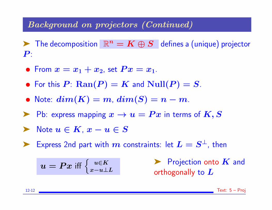
Background on projectors (Continued)

ä The decomposition Rn = K ⊕ S defines a (unique) projectorP :

• From x = x1 + x2, set Px = x1.

• For this P : Ran(P ) = K and Null(P ) = S.

• Note: dim(K) = m, dim(S) = n−m.

ä Pb: express mapping x→ u = Px in terms of K,S

ä Note u ∈ K, x− u ∈ S

ä Express 2nd part with m constraints: let L = S⊥, then

u = Px iff{

u∈Kx−u⊥L

ä Projection onto K andorthogonally to L


��

��

��

��

��

��

��

��

��

��

��

KL

HHHH

HHH

HHH

HHH

HHH

HH

HHH

HHH

HHH

HHH

HHH

HHH

x

��HH

��

��

��

��Px

��

ä Illustration: P projects onto K and orthogonally to L

ä When L = K projector is orthogonal.

ä Note: Px = 0 iff x ⊥ L.


Projection methods

ä Initial Problem: b−Ax = 0

Given two subspaces K and L of RN define the approximate prob-lem:

Find x̃ ∈ K such that b−Ax̃ ⊥ L

ä Petrov-Galerkin condition

ä m degrees of freedom (K) + m constraints (L)→

ä a small linear system (‘projected problem’)

ä This is a basic projection step. Typically a sequence of such stepsare applied


ä With a nonzero initial guess x0, approximate problem is

Find x̃ ∈ x0 +K such that b−Ax̃ ⊥ L

Write x̃ = x0 + δ and r0 = b−Ax0. → system for δ:

Find δ ∈ K such that r0 −Aδ ⊥ L

- Formulate Gauss-Seidel as a projection method -

- Generalize Gauss-Seidel by defining subspaces consisting of ‘blocks’of coordinates span{ei, ei+1, ..., ei+p}


Matrix representation:

Let•V = [v1, . . . , vm] a basis of K &

•W = [w1, . . . , wm] a basis of L

ä Write approximate solution as x̃ = x0 + δ ≡ x0 + V y wherey ∈ Rm. Then Petrov-Galerkin condition yields:

W T(r0 −AV y) = 0

ä Therefore,

x̃ = x0 + V [W TAV ]−1W Tr0

Remark: In practice W TAV is known from algorithm and has asimple structure [tridiagonal, Hessenberg,..]


Prototype Projection Method

Until Convergence Do:

1. Select a pair of subspaces K, and L;

2. Choose bases:V = [v1, . . . , vm] for K andW = [w1, . . . , wm] for L.

3. Compute :r ← b−Ax,y ← (W TAV )−1W Tr,

x← x+ V y.


Projection methods: Operator form representation

ä Let Π = the orthogonal projector onto K andQ the (oblique) projector onto K and orthogonally to L.

Πx ∈ K, x−Πx ⊥ KQx ∈ K, x−Qx ⊥ L

��

��

��

��

��

K

L

HHHHH

HHH

HH

HHHHH

HHH

HH

?

x

Πx��

��

��

Qx

��

Π and Q projectors

Assumption: no vector of K is ⊥ to L


In the case x0 = 0, approximate problem amounts to solving

Q(b−Ax) = 0, x ∈ K

or in operator form (solution is Πx)

Q(b−AΠx) = 0

Question: what accuracy can one expect?


ä Let x∗ be the exact solution. Then

1) We cannot get better accuracy than ‖(I −Π)x∗‖2, i.e.,

‖x̃− x∗‖2 ≥ ‖(I −Π)x∗‖2

2) The residual of the exact solution for the approximate problemsatisfies:

‖b−QAΠx∗‖2 ≤ ‖QA(I −Π)‖2‖(I −Π)x∗‖2


Two Important Particular Cases.

1. L = K

ä When A is SPD then ‖x∗ − x̃‖A = minz∈K ‖x∗ − z‖A.

ä Class of Galerkin or Orthogonal projection methods

ä Important member of this class: Conjugate Gradient (CG) method

2. L = AK .

In this case ‖b−Ax̃‖2 = minz∈K ‖b−Az‖2

ä Class of Minimal Residual Methods: CR, GCR, ORTHOMIN,GMRES, CGNR, ...


One-dimensional projection processes

K = span{d}and

L = span{e}

Then x̃ = x+ αd. Condition r −Aδ ⊥ e yields

α = (r,e)(Ad,e)

ä Three popular choices:

(1) Steepest descent

(2) Minimal residual iteration

(3) Residual norm steepest descent


1. Steepest descent.

A is SPD. Take at each step d = r and e = r.

Iteration:r ← b−Ax,α← (r, r)/(Ar, r)x← x+ αr

ä Each step minimizes f(x) = ‖x−x∗‖2A = (A(x−x∗), (x−

x∗)) in direction −∇f .

ä Convergence guaranteed if A is SPD.

- As is formulated, the above algorithm requires 2 ‘matvecs’ perstep. Reformulate it so only one is needed.


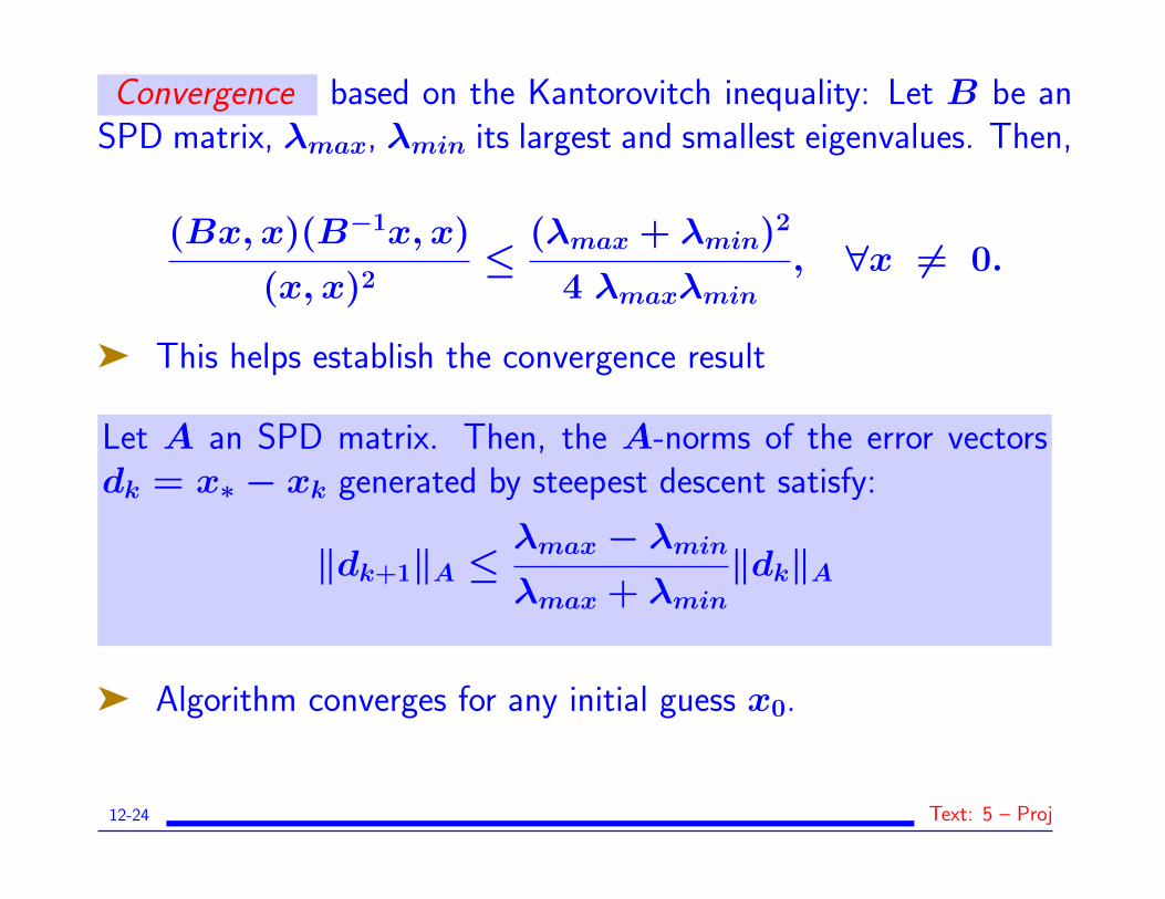
Convergence based on the Kantorovitch inequality: Let B be anSPD matrix, λmax, λmin its largest and smallest eigenvalues. Then,

(Bx, x)(B−1x, x)

(x, x)2≤

(λmax + λmin)2

4 λmaxλmin, ∀x 6= 0.

ä This helps establish the convergence result

Let A an SPD matrix. Then, the A-norms of the error vectorsdk = x∗ − xk generated by steepest descent satisfy:

‖dk+1‖A ≤λmax − λminλmax + λmin

‖dk‖A

ä Algorithm converges for any initial guess x0.


Proof: Observe ‖dk+1‖2A = (Adk+1, dk+1) = (rk+1, dk+1)

ä by substitution,

‖dk+1‖2A = (rk+1, dk − αkrk)

ä By construction rk+1 ⊥ rk so we get ‖dk+1‖2A = (rk+1, dk).

Now:

‖dk+1‖2A = (rk − αkArk, dk)

= (rk, A−1rk)− αk(rk, rk)

= ‖dk‖2A

(1−

(rk, rk)

(rk, Ark)×

(rk, rk)

(rk, A−1rk)

).

Result follows by applying the Kantorovich inequality.


2. Minimal residual iteration.

A positive definite (A+AT is SPD). Take at each step d = r ande = Ar.

Iteration:r ← b−Ax,α← (Ar, r)/(Ar,Ar)x← x+ αr

ä Each step minimizes f(x) = ‖b−Ax‖22 in direction r.

ä Converges under the condition that A+AT is SPD.

- As is formulated, the above algorithm would require 2 ’matvecs’at each step. Reformulate it so that only one matvec is required


Convergence

Let A be a real positive definite matrix, and let

µ = λmin(A+AT)/2, σ = ‖A‖2.

Then the residual vectors generated by the Min. Res. Algorithmsatisfy:

‖rk+1‖2 ≤(

1−µ2

σ2

)1/2

‖rk‖2

ä In this case Min. Res. converges for any initial guess x0.


Proof: Similar to steepest descent. Start with

‖rk+1‖22 = (rk − αkArk, rk − αkArk)

= (rk − αkArk, rk)− αk(rk − αkArk, Ark).

By construction, rk+1 = rk−αkArk is ⊥ Ark. ä ‖rk+1‖22 =

(rk − αkArk, rk). Then:

‖rk+1‖22 = (rk − αkArk, rk)

= (rk, rk)− αk(Ark, rk)

= ‖rk‖22

(1−

(Ark, rk)

(rk, rk)

(Ark, rk)

(Ark, Ark)

)= ‖rk‖2

2

(1−

(Ark, rk)2

(rk, rk)2

‖rk‖22

‖Ark‖22

).

Result follows from the inequalities (Ax, x)/(x, x) ≥ µ > 0 and‖Ark‖2 ≤ ‖A‖2 ‖rk‖2.


3. Residual norm steepest descent.

A is arbitrary (nonsingular). Take at each step d = ATr ande = Ad.

Iteration:r ← b−Ax, d = ATrα← ‖d‖2

2/‖Ad‖22

x← x+ αd

ä Each step minimizes f(x) = ‖b−Ax‖22 in direction −∇f .

ä Important Note: equivalent to usual steepest descent applied tonormal equations ATAx = ATb .

ä Converges under the condition that A is nonsingular.


relaxation methods: jacobi, gauss-seidel, sor basic … · ä jacobi and gauss-seidel converge for...

Documents