reliability engineering lec notes #8 notes74_92

7/30/2019 Reliability Engineering Lec Notes #8 notes74_92

http://slidepdf.com/reader/full/reliability-engineering-lec-notes-8-notes7492 1/19



75

Determine the probability that a repair will be completed in 6 h. What is the MTTR?

What is the median time to repair (t med )?

Solution

Pr{T < 6} = H (6) =6

0

∫ dt h(t ) =6

1

∫ dt t 2

333=

1

(3)(333)t 3

6

1

= 0. 215

MTTR =

∞

0

∫ dt t h(t ) =

10

1

∫ dt t 3

333=

1

(4)(333)t 4

10

1

= 7. 51 h

t med

0∫ dt h(t ) = 0. 5 =>

t med

1∫ dt

t 2

333

= 0. 5 =>1

(3)(333)

t 3

t med

1

= 0. 5 => t med = 7. 94 h

1 2 3 4 5 6 7 8 9 100

0.05

0.1

0.15

0.2

0.25

0.3

0.35

t(hours)

h ( t )

MTTR tmed

1 2 3 4 5 6 7 8 9 100

0.1

0.2

0.3

0.4

0.5

0.6

0.7

0.8

0.9

1

t(hours)

H ( t )

MTTR tmed

Some commonly used repair time distributions are:

Exponential: h(t ) =1

MTTRe− t / MTTR:

Lognormal: h(t ) =

1

√ 2π ts exp

−

1

2

[ln(t / t med )]2

s2

An exponential repair time distribution indicates that repair rate is constant, i.e. the prob-

ability that the repair will be completed within [t , t + dt ] but not before t , is the same for

all t . A lognormal repair time distribution indicates that most repair times will be dis-

tributed around the maximum of the distribution with a relatively few long repair times in

the right-hand tail of the distribution.



76

Maintenance as a Stochastic Point Process

A stochastic point process is characterized by events occurring at isolated instants dis-

tributed stochastically in time. Let

T k : time at which k

th

failure occurs, and,

X k : time between failures, i.e. X k = T k − T k −1

and assume that downtime is negligible compared to X k . Then maintenance can be

regarded as a stochastic point process, with

T k =k

i=1Σ X i and E (T k ) =

k

i=1Σ E ( X i),

E ( X i): Mean time between ith and i − 1st failure.

The probability that there will be exactly j number of failures up to time t can be found

from

Pr{ j} = Pr{T j+1 ≥ t } − Pr {T j ≥ t }

Renewal Process

If X i are statistically independent and are identically distributed, maintenance can be

modeled as a renewal process (e.g. if repair restores the unit to "as good as new condi-

tion"). In this situation,

E (T k ) = k E ( X 1) = k µ 1, Var (T k ) = k Var ( X 1) = k σ 21

and

Pr{T k ≤ t } ≈ Φ

t − k µ 1

σ 1√ k

=1

√ 2π

t − k µ 1

σ 1√ k

−∞∫ dz e− z2 /2 =

1

2

1 + erf

t − k µ 1

σ 1√ 2k

where

erf ( x) = 2√ π

x

0∫ du e−u2 /2.

The last relation follows from the Central Limit Theorem and holds for k > 30 for arbi-

trary distributions of T k . It is exact if all X k have normal distributions, as can be shown

fairly simply using moment generating functions.



77

If p( X i) = e−λ t for all i, the renewal process is called Homogeneous Poisson Process. In

this situation,

Pr {T k ≤ t } = 1 − e−λ t r −1

i=0

Σ

(λ t )i

i!

as shown earlier. The figures below compare how the normal distribution

Φ[(t − k µ 1)/(σ 1√ k )] approximates this distribution for various k .

0 1 2 3 4 5 6 7 8 9 100

0.1

0.2

0.3

0.4

0.5

0.6

0.7

0.8

0.9

1

lambda*t

P r { T k < t }

f o r k = 5

__ Poisson

−− Normal

0 5 10 150

0.1

0.2

0.3

0.4

0.5

0.6

0.7

0.8

0.9

1

lambda*t

P r { T k < t }

f o r k = 1 0

__ Poisson

−− Normal

k=5 k=10

0 5 10 15 20 250

0.1

0.2

0.3

0.4

0.5

0.6

0.7

0.8

0.9

1

lambda*t

P r { T k < t } f o r k = 1 5

__ Poisson

−− Normal

0 5 10 15 20 25 300

0.1

0.2

0.3

0.4

0.5

0.6

0.7

0.8

0.9

1

lambda*t

P r { T k < t } f o r k = 2 0

__ Poisson

−− Normal

k=15 k=20

Minimal Repair Process

If the repair consists of restoring the unit or system just to operation, possibly in a

degraded state, then the time between failures will no longer be statistically independent

and identically distributed. Such a process can be also modeled as a stochastic point pro-

cess by defining an intensity function, ρ (t ) as



78

ρ (t ) ≡dE [ N (t )]

dt ≈

N (t + ∆t ) − N (t )

∆t

where N (t ) is the number of failures until time t . Then

E [ N (t )] =

t

0∫ dt ′ ρ (t ′)

and the mean time between failures (MTBF) is

MTBF =1

ρ (t )

or MTBF for an interval t 1 ≤ t ≤ t 2 is

MTBF(t 1, t 2) =t 2 − t 1

E [ N (t 2

)] − E [ N (t 1

)].

Note that MTBF is different from MTTF which is the mean time to first failure. Two

common distributions used for describing ρ (t ) are

ρ (t ) = a bt b−1

and

ρ (t ) = ea+bt .

Preventive Maintenance

The purpose of preventive maintenance is to restore the component to "as good as

new" condition (e.g. replace) at scheduled intervals. This type of maintenance is worth-

while if the component has increasing failure rate (e.g. mechanical devices). Let

T M : maintenance interval

Ak (t ): event that the component fails for the first time within dt at time t during kT m ≤ t < (k + 1)T m

Bk : event that the component survives until time t = kT M

and assume that the duration of the maintenance is negligibly small. Then

Pr{ Ak (t )} = Pr{ Ak (t )| Bk } Pr{ Bk }

or

f *(t ) =∞

k =0Σ [ H (t − kT M ) − H (t − (k + 1)T M )] f (t ) R

k (T M )

where H (t ) is the Heaviside step function, f *(t ) is the failure pdf of the component after

after incorporating preventive maintenance, f (t ) failure pdf of the new component and

R(t ) is the reliability function of the new component.



79

Example 2

Let

f (t ) = 0. 25/year 0 ≤ t < 4 years.

If the component is replaced every year, find f *(t ).

Solution

For f (t ) = 0. 25/year,

F (t ) = 0. 25t => R(t ) = 1 − 0. 25t 0 ≤ t < 4 years.

λ (t ) =f (t )

1 − F (t )=> λ (t ) =

0. 25

1 − 0. 235t =

1

4 − t 0 ≤ t < 4 years.

Since T M = 1 year, R(T M ) = 0.75 and

f *(t ) = 0. 25∞

k =0Σ [ H (t − k ) − H (t − (k + 1))]0. 75k

Note that the average hazard λ * rate for f *(t ) is

λ * =

1

0

∫ dt

4 − t = 0. 2877/ year

The figure below shows that the f *(t ) can be approximated as an exponential distribution

with λ *.

0 2 4 6 8 10 120

0.05

0.1

0.15

0.2

0.25

0.3

0.35

t(years)

f *(

t )

++ Exact

__ f*(t)=0.2887exp(−0.2887*t)



80

State-Dependent Systems With Repair

We will extend the Markov modeling approach described earlier to to analyze state-

dependent transitions with repair. In order to illustrate the approach, we will again use

the system which has identical 2 bi-state components (i.e. good or failed). The system is

good if both components are good and is degraded if only 1 component is good. The

components fail randomly with failure rate λ .

Possible system states are as shown in the table below.

System State Component#1 Component#2

0 g g

1 g f

2 f g

3 f f

System states 1 and 2 correspond to degraded operation. We will also assume:

• when a component fails repair starts immediately,

• there is one repairman, and,

• both components have repair times with identical exponential distributions, i.e.

µ ∆t ≡ Pr{repair is completed at t + ∆t |component is failed at t } = ∆t /MTTR

(or µ = 1/MTTR) for both components.

We first note that since the failure of either component implies degraded operation

and both components have the same failure and repair rates States 1 and 2 can be com-

bined into a single State 12 as before but now with the state indices indicating

0: Both components good

12: One component good and under repair

3: 1 component failed and 1 under repair



81

0 12 3

µ µ

2λ λ

There is no transition from State 3 to State 1, because there is only 1 repairman.

The Markov model is

dp0(t )

dt = − 2λ p0(t ) + µ p12(t )

dp12(t )

dt = 2λ p0(t ) − (λ + µ ) p12(t ) + µ p3(t )

dp3(t )

dt = λ p12(t ) − µ p3(t )

with p0(0) = 1 and p12(0) = p3(0) = 0. These equations can be solved analytically using

Laplace transforms, i.e.

s ˜ p0(s) − 1 = − 2λ ˜ p0(s) + µ ˜ p12(s)

s ˜ p12(s) = 2λ ˜ p0(s) − (λ + µ ) ˜ p12(s) + µ ˜ p3(s)

s ˜ p3(s) = λ ˜ p12(s) − µ ˜ p3(s)

=> ˜ p0(s) =µ

2 + λ s + 2 µ s + s2

s[s2 + s(3λ + 2 µ ) + 2λ 2 + 2λ µ + µ 2]=

µ 2 + λ s + 2 µ s + s2

s(s − r 1)(s − r 2)

˜ p12(s) =2λ (s + µ )

s[s2 + s(3λ + 2 µ ) + 2λ 2 + 2λ µ + µ 2]=

2λ (s + µ )

s(s − r 1)(s − r 2)

˜ p3(s) =2λ 2

s[s2 + s(3λ + 2 µ ) + 2λ 2 + 2λ µ + µ 2]=

2λ 2

s(s − r 1)(s − r 2)

where



82

r 1 = −3

2λ − µ +

1

2√ λ 2 + 4λ µ , r 2 = −

3

2λ − µ −

1

2√ λ 2 + 4λ µ .

=> p0(t ) =µ 2

r 1r 2 +

er 1t r 1λ + 2r 1 µ + r 21 + µ 2

r 1(r 1 − r 2) −

er 2t r 2λ + 2r 2 µ + µ 2 + r 22

r 2(r 1 − r 2)

p12(t ) = 2λ

µ

r 1r 2+

er 1t ( µ + r 1)

r 1(r 1 − r 2)−

er 2t ( µ + r 2)

r 2(r 1 − r 2)

p3(t ) = 2λ 2

1

r 1r 2+

er 1t

r 1(r 1 − r 2)−

er 2t

r 2(r 1 − r 2)

We note that

r 1r 2 =

3

2λ + µ

2

− λ 2 + 4λ µ = 2λ 2 + 2λ µ + µ 2.

Thus both r 1 and r 2 are negative and for large times we get

t →∞lim ˜ p0(t ) =

µ 2

2λ 2 + 2λ µ + µ 2

t →∞lim ˜ p12(t ) =

2λ µ

2λ 2 + 2λ µ + µ 2

t →∞lim ˜ p3(t ) = 2λ 2

2λ 2 + 2λ µ + µ 2

The same results could have been obtained using

•s→0lim s ˜ pi(s) =

t →∞lim pi(t ) (i = 0, 12, 3), or from

•dpi(t )

dt = 0 (i = 0, 12, 3) with p0(∞) + p12(∞) + p3(∞) = 1

Finding MTTF state-dependent systems with repair needs special treatment. In order to

illustrate the need, again consider the above system with identical 2 bi-state components

and 1 repairman. From the definition of MTTF we should have

MTTF =

∞

0

∫ dt t λ p12(t )

which yields infinity because since there are an infinite number of transitions into the

failed State 3. In order to find MTTF, the failed state needs to be defined as an absorbing

state, i.e. once the system arrives in the failed state, it stays there forever. The Markov



83

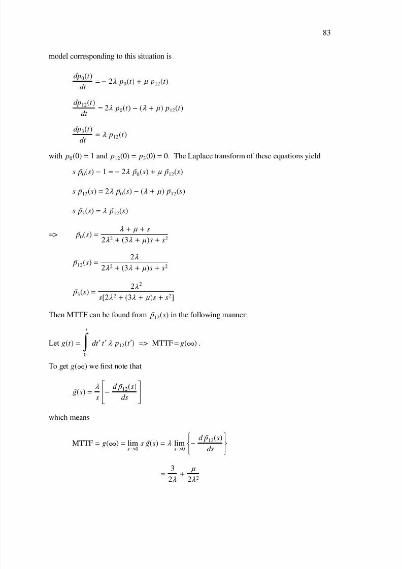
model corresponding to this situation is

dp0(t )

dt = − 2λ p0(t ) + µ p12(t )

dp12(t )

dt = 2λ p0(t ) − (λ + µ ) p12(t )

dp3(t )

dt = λ p12(t )

with p0(0) = 1 and p12(0) = p3(0) = 0. The Laplace transform of these equations yield

s ˜ p0(s) − 1 = − 2λ ˜ p0(s) + µ ˜ p12(s)

s ˜ p12(s) = 2λ ˜ p0(s) − (λ + µ ) ˜ p12(s)

s ˜ p3(s) = λ ˜ p12(s)

=> ˜ p0(s) =λ + µ + s

2λ 2 + (3λ + µ )s + s2

˜ p12(s) =2λ

2λ 2 + (3λ + µ )s + s2

˜ p3(s) =2λ 2

s[2λ 2

+ (3λ + µ )s + s2

]

Then MTTF can be found from ˜ p12(s) in the following manner:

Let g(t ) =

t

0

∫ dt ′ t ′ λ p12(t ′) => MTTF = g(∞) .

To get g(∞) we first note that

˜ g(s) =λ

s

−

d ˜ p12(s)

ds

which means

MTTF = g(∞) =s−>0lim s ˜ g(s) = λ

s−>0lim

−

d ˜ p12(s)

ds

=3

2λ +

µ

2λ 2



84

Av ailability

Av ailability is the counterpart of reliability for maintained systems. In general,

Av ailability =uptime

uptime + downtime.

The point or instantaneous availability, A(t ), is defined as the probability of the system

performing its design function or mission at a specified time t . Interval availability is the

probability that the system will perform its design function or mission over a specified

time period.

• Average availability over the time period [0,T ] is

Aav(T ) =1

T

T

0∫ dt A(t ).

• Mission or interval availability over the time period [t 2 − t 1] is

Aav(t 2 − t 1) =1

t 2 − t 1

t 2

t 1

∫ dt A(t ).

• Steady-state or equilibrium availability is

A = t →∞lim A(t ).

To illustrate these definitions, consider the system which has identical 2 bi-state

components and 1 repairman, i.e.

dp0(t )

dt = − 2λ p0(t ) + µ p12(t )

dp12(t )

dt = 2λ p0(t ) − (λ + µ ) p12(t ) + µ p3(t )

dp3(t )dt

= λ p12(t ) −ν p3(t ), p0(0) = 1, p12(0) = p3(0) = 0.

0: both components good

12: one component good and under repair

1: component failed and 1 under repair

This system can be regarded as an example of systems with exponential failure and repair

distributions, as well as as an example of systems with standby components and perfect



85

switching. We hav e shown that

p0(t ) =µ

2

r 1r 2+

er 1t r 1λ + 2r 1 µ + r 21 + µ

2

r 1(r 1 − r 2)−

er 2t r 2λ + 2r 2 µ + µ

2 + r 22

r 2(r 1 − r 2)

p12(t ) = 2λ

µ

r 1r 2+

er 1t ( µ + r 1)

r 1(r 1 − r 2)−

er 2t ( µ + r 2)

r 2(r 1 − r 2)

p3(t ) = 2λ 2

1

r 1r 2+

er 1t

r 1(r 1 − r 2)−

er 2t

r 2(r 1 − r 2)

where

r 1

= −3

2λ − µ +

1

2 √ λ 2 + 4λ µ , r

2

= −3

2λ − µ −

1

2 √ λ 2 + 4λ µ .

States 0 and 12 are the "up" states, i.e. states at which the system performs its design

function or mission and State 3 is the "down" state. We will now let x = µ / λ

=> r 1 = − λ

3

2+ x −

1

2√ 1 + 4 x

, r 2 ≈ − λ

3

2+ x +

1

2√ 1 + x

or

r 1 = − λ f 1( x), r 2 = − λ f 2( x)

where

f 1( x) =3

2+ x −

1

2√ 1 + 4 x, f 2( x) =

3

2+ x +

1

2√ 1 + 4 x.

=> p0(t , x) =x2

f 1( x) f 2( x)−

e−λ t f 1( x)

f 1( x) + 2 x f 1( x) − f 21 ( x) − x2

f 1( x)[ f 1( x) − f 2( x)]

+

e−λ t f 2( x)

f 2( x) + 2 x f 2( x) − f 22 ( x) − x2

f 2( x)[ f 1( x) − f 2( x)]

p12(t , x) = 2

x

f 1( x) f 2( x)+

e−λ t f 1( x)[ x − f 1( x)]

f 1( x)[ f 1( x) − f 2( x)]−

e−λ t f 2( x)( x − f 2( x))

f 2( x)[ f 1( x) − f 2( x)]

p3(t , x) = 2

1

f 1( x) f 2( x)+

e−λ t f 1( x)

f 1( x)[ f 1( x) − f 2( x)]−

e−λ t f 2( x)

f 2( x)[ f 1( x) − f 2( x)]



86

Then point or instantaneous availability is

A(t , x) = p0(t , x) + p12(t , x),

average availability over the time period [0, t ] is

Aav(t , x) =1

t

t

0

∫ dt ′ [ p0(t ′, x) + p12(t ′, x)]

and steady-state availability is

A( x) =x2

f 1( x) f 2( x)+

2 x

f 1( x) f 2( x).

0 0.2 0.4 0.6 0.8 1 1.2 1.4 1.6 1.8 20.94

0.95

0.96

0.97

0.98

0.99

1

lambda*t

A v a i l a b i l i t y

x=5

x=10

x=15

__ Point or instantaneous

−− Steady−state

−. Average

Note that:

• Availability increases with increasing x = µ / λ

• Average availability is larger than instantaneous availability.

• x→∞lim Aav(t ) → A(t ) → 1 since the component is instantly repaired (i.e. becomes

good-as-new).



87

Tw o important aspect of systems with standby components are: a) switching may

not be perfect since the standby component may have failed while in standby, and,

b) failure of the standby component will not discovered until inspection time. To

illustrate these aspects, we will use the Markov approach with the previous example

system with 2 identical bi-state components and 1 repairman, but now assume the

following:

1. Under normal operation, Component 1 is on and Component 2 is in standby

2. Component 2 comes on-line if Component 1 fails (failure rate λ )

3. Component 2 may fail in standby (failure rate λ s) or while operating (failure rate λ )

4. Component 2 is inspected every T time units. Inspection time is negligible but if

Component 2 is found failed during inspection, it is restored to good-as-new state

with repair rate µ .

5. If Component 1 fails and Component 2 comes on-line, repair starts immediately,

Component 1 is restored to good-as-new state with repair rate µ and Component 2 is

put in standby when Component 1 repair is completed.

6. If Component 1 fails and Component 2 does not come on-line (i.e. standby failure

not discovered), repair starts on Component 1 first, Component 1 is restored to

good-as-new operational state with repair rate µ .

7. If Component 2 is under repair when Component 1 fails, Component 1 repair does

not start until Component 2 repair is completed.

8. System is available if either Component 1 or Component 2 is on.



88

System states relevant for availability analysis are the following:

0: Component 1 is on, Component 2 is in standby and good

1: Component 1 is on, Component 2 is in standby and failed

2: Component 1 is on, Component 2 is under repair.

3: Component 1 is failed, Component 2 is under repair.

4: Component 1 is under repair, Component 2 is on.

5: Component 1 is under repair, Component 2 is failed.

2

4

5

µ

λ

µ

λ

3

µ

λ

1

λ

δ ( t −

k T )

µ

λs

0

dp0

dt = − (λ s + λ ) p0(t ) + µ p2(t ) + µ p4(t )

dp1

dt = λ s p0(t ) − [λ +δ (t − kT )] p1(t )

dp2

dt =δ (t − kT ) p1(t ) − ( µ + λ ) p2(t ) + µ p5(t )

dp3

dt = λ p2(t ) − µ p3(t )

dp4

dt = λ p0(t ) + µ p3(t ) − ( µ + λ ) p4(t )

dp5

dt = λ p1(t ) + λ p4(t ) − µ p5(t )

or equivalently



89

dpk 0

dt = − (λ s + λ ) pk

0(t ) + µ pk 2(t ) + µ pk

4(t )

dpk 1

dt = λ s p

k 0(t ) − λ pk

1(t )

dpk 2

dt = − ( µ + λ ) pk

2(t ) + µ pk 5(t )

dpk 3

dt = λ pk

2(t ) − µ pk 3(t )

dpk 4

dt = λ pk

0(t ) + µ pk 3(t ) − ( µ + λ ) pk

4(t )

dpk

5

dt = λ p1(t ) + λ p4(t ) − µ pk

5(t )

for (k − 1)T < t < kT (k = 1, 2, . . . ) with p00(0) = 1, p0

i (0) = 0, i = 1, 2, 3, 4, 5,

pk 1(kT ) − pk −1

1 (kT ) = −pk −1

1 (kT ) + pk 1(kT )

2=> pk

1(kT ) =1

3 pk −1

1 (kT )

pk 2(kT ) − pk −1

2 (kT ) =pk −1

1 (kT ) + pk 1(kT )

2=> pk

2(kT ) = pk −12 (kT ) +

2

3 pk −1

1 (kT )

and pk i (kT ) = pk −1

i (kT ) i = 1, 3, 4, 5.

For a parametric study, it is more convenient to express these equations in dimensionless

time x = λ t with ε = λ s / λ and r = µ / λ which yields

dpk 0

dx= − (ε + 1) pk

0( x) + rpk 2( x) + rpk

4( x)

dpk 1

dx= ε pk

0( x) − pk 1( x)

dpk 2

dx

= − (r + 1) pk 2( x) + rpk

5( x)

dpk 3

dx= pk

2( x) − rpk 3( x)

dpk 4

dx= pk

0( x) + rpk 3( x) − (r + 1) pk

4( x)



90

dpk 5

dx= pk

1( x) + pk 4( x) − rpk

5( x)

for kX < t < (k + 1) X (k = 0, 1, 2, . . . ) with p00(0) = 1, p0

i (0) = i = 1, 2, 3, 4, 5 and for

k ≥ 1

pk 1( X ) =

1

3 pk −1

1 ( X )

pk 2( X ) = pk −1

2 ( X ) +2

3 pk −1

1 ( X )

pk i ( X ) = pk −1

i ( X ) i = 0, 3, 4, 5.

From the system definition,

A( X ) = pk 0( X ) + pk

1( X ) + pk 2( X ) + pk

4( X ).

The steady-state availability can be found from the solution of the equations

0 = − (ε + 1) p0 + rp2 + rp4

0 = ε p0 − p1

0 = − (r + 1) p2 + rp5

0 = p2 − rp3

0 = p0 + rp3 − (r + 1) p4

1 = p0 + p1 + p2 + p3 + p4 + p5,

where pi = pi(∞), which yields

p0 = r 2 / d , p1 = ε r 2 / d , p2 = r (1 + r ε + ε )/ d

p3 = (1 + r ε + ε )/ d , p4 = r (1 + r + ε )/ d , p5 = (r + 1)(1 + r ε + ε )/ d

with

d = 3 r 2 + 3 r + 4 r 2 ε + 5 r ε + r 3 + r 3 ε + 2 + 2 ε

=> A(r , ε ) = p0 + p1 + p2 + p4



91

00.2

0.40.6

0.81

0

0.2

0.4

0.6

0.8

10

0.1

0.2

0.3

0.4

0.5

epsilonr

A v a i l a b i l i t y

Note that:

• A(r , ε ) = 0 f o r r = µ / λ = 0. If the system is not repaired it will eventually fail

• A(r , ε ) reaches a maximum for r = 1 and ε = λ s / λ = 0 as expected intuitively.

Design Tradeoff Analysis

Suppose steady-state availability A of a system/component is specified. Such aspecification may arise out of regulatory constraints (e.g. nuclear reactors, airplanes), cus-

tomer demands (e.g. car industry) or mission requirements (e.g. satellites, military hard-

ware). The design problem to be solved is how to find the optimum mean-time-to-repair

(MTTR) and mean-time-between-failures (MTBF) so that the cost is minimized. Then

the MTTR and MTBF can be used as design constraints to design the system or to select

the component.

Let

x = MTBF

y = MTTR

C x( x) = Cost of system/component as a function of MTBF

C y( y) = Cost of downtime for the system/component

MTBF = Minimum allowed MTBF

MTTR = Minimum MTTR

MTTR = Maximum MTTR



92

Since MTTR does not usually include waiting times (e.g. due to lack of stock), from the

general description of availability we have

A ≤x

x + y=> (1 − A) x − A y ≥ 0.

Then the problem is

minimize z = C x( x) + C y( y)

subject to (1 − A) x − A y ≥ 0

MTBF < x

MTTR ≤ y ≤ MTTR

Example 3

minimize z = C x( x) + C y( y) = 10 x + 5000 − 200 y

subject to (1 − A) x − A y = 0. 05 x − 0. 95 y ≥ 0

200 = MTBF < x

5 = MTTR ≤ y ≤ MTTR = 24

This is a linear programming problem with the solution laying at the intersection of con-

straint pairs.

MTTR (h)

MTBF (h)

100 200 300 400 500

10

20

30

40

50

0 x

y

0. 0 5 x

− 0. 9 5

y = 0

−10

z = 1 0

x + 5 0

0 0 − 2

0 0 x

D i r e c t i o

n o f d

e c r e a s i n

g z

Optimal Solution

(456,24)

reliability engineering lec notes #8 notes74_92

Documents