reliable computation of equilibrium states and bifurcations in food

Reliable Computation of Equilibrium States and

Bifurcations in Food Chain Models

C. Ryan Gwaltney, Mark P. Styczynski †, and Mark A. Stadtherr*

Department of Chemical and Biomolecular Engineering

University of Notre Dame

182 Fitzpatrick Hall

Notre Dame, IN 46556

USA

†Current Address: Department of Chemical Engineering, Massachusetts Institute of Technology, Building 66, 25 Ames Street, Cambridge MA 02139 USA

*Author to whom correspondence should be addressed: Tel.: (574) 631-9318, Fax: (574) 631-8366, E-mail: [email protected]

(July 2003)

(revised, March 2004)

Abstract

Food chains and webs in the environment can be modeled by systems of ordinary

differential equations that approximate species or functional feeding group behavior with

a variety of functional responses. We present here a new methodology for computing all

equilibrium states and bifurcations of equilibria in food chain models. The methodology

used is based on interval analysis, in particular an interval-Newton/generalized-bisection

algorithm that provides a mathematical and computational guarantee that all roots of a

nonlinear equation system are enclosed. The procedure is initialization-independent, and

thus requires no a priori insights concerning the number of equilibrium states and

bifurcations of equilibria or their approximate locations. The technique is tested using

several example problems involving tritrophic food chains.

Keywords: Food chain; Ecology, Nonlinear dynamics; Bifurcations; Interval analysis

1

1. INTRODUCTION Food chains and webs in the environment are highly complex and interdependent

systems. Seemingly insignificant changes in the parameters of such systems can have drastic

consequences. Food chains and webs can be modeled by systems of ordinary differential

equations that approximate species or functional feeding group behavior with a variety of

functional responses. Many simple two-species models have been thoroughly explored, while

new discoveries continue to be made in examining models with three and four trophic levels

(e.g., Moghadas and Gumel, 2003). Ecological systems exhibit complex interdependencies in

that changes in a single trophic level may have far reaching impacts on the rest of the system. In

some cases, this leads to unexpected or counterintuitive behavior. Use of simple food chain

models can assist in qualitatively illustrating the complexity and interdependencies in real

ecological systems.

Our interest in ecological modeling is motivated by its use as one tool in studying the

impact on the environment of the industrial use of newly discovered materials. Clearly it is

preferable to take a proactive, rather than reactive, approach when considering the safety and

environmental consequences of using new compounds. Of particular interest is the potential use

of room temperature ionic liquid (IL) solvents in place of traditional solvents (Brennecke and

Maginn, 2001). IL solvents have no measurable vapor pressure and thus, from a safety and

environmental viewpoint, have several potential advantages relative to the traditional volatile

organic compounds (VOCs) used as solvents, including elimination of hazards due to inhalation,

explosion and air pollution. However, ILs are, to varying degrees, soluble in water; thus, if they

are used industrially on a large scale, their entry into the environment via aqueous waste streams

is of concern. The effects of trace levels of ILs in the environment are today essentially

unknown and thus must be studied. Single species toxicity information is very important as a

basis for examining the effects that a contaminant will have on an environment. However, this

information, when considered by itself, is insufficient to predict impacts on a food chain, food

web, or an ecosystem. Ecological modeling provides a means for studying the impact of such

perturbations on a localized environment by focusing not just on the impact on one species, but

rather on the larger impacts on the food chain and ecosystem. Of course, ecological modeling is

just one part of a much larger suite of tools, including toxicological (Jastorff et al., 2003;

2

Freemantle, 2002), hydrological and microbiological studies, that must be used in addressing this

issue.

In this paper, we concentrate on the computation of equilibrium states (steady states) in

food chain models, and on the computation of bifurcations of equilibria. A bifurcation is a

sudden, macroscopic change in the qualitative behavior of a system as some parameter is varied.

These changes include the appearance and disappearance of equilibrium states (fold or saddle

node bifurcation), the exchange of stability of two equilibria (transcritical bifurcation), and the

change of stability of an equilibrium point (Hopf bifurcation). van Coller (1997) provides a good

high-level introduction for dynamical systems and their characteristics, while a more advanced

and thorough review of bifurcations can be found in Kuznetsov (1998). For simple systems, or

specific parts of more complex ones, analytic techniques and isocline analysis are useful for

analysis of equilibrium states and bifurcations. However, for more complex problems,

continuation methods are the predominant computational tools, with packages such as AUTO

(Doedel et al., 1997) and others (van Coller, 1997) being particularly popular in this context.

These are applied to solve the systems of nonlinear algebraic equations that represent the

equilibrium states and bifurcations.

Continuation methods can be quite reliable, especially in the hands of an experienced

user. However, in general, continuation methods are initialization dependent, and may fail to

find all solutions to a system of nonlinear equations. Thus, in this context, these methods may

fail to find all equilibrium states or all bifurcations of equilibria. In this paper, we propose a new

approach for computing equilibrium states and bifurcations of equilibria in food chain models,

and consider the feasibility of using this approach. This technique is based on interval

mathematics, in particular an interval-Newton approach combined with generalized bisection,

and provides a mathematical and computational guarantee that all equilibrium states and

bifurcations of equilibria will be located (or, more precisely, enclosed within a very narrow

interval). There are other dynamical features of interest, such as limit cycles (and their

bifurcations); however, our attention here will be limited to equilibrium states and their

bifurcations. While the focus here is on food chain models, there are clearly applications of this

technique in the analysis of other dynamical systems of interest in chemical engineering.

In the next section, we describe the development of food chain models and the

formulation of the nonlinear equation systems that must be solved to determine equilibrium

3

states and bifurcations. In Section 3, the computational method to be considered is described

briefly. Then, in Section 4, we apply this methodology to some relatively simple systems to

explore its feasibility.

2. PROBLEM FORMULATION

2.1 Food Chain Models

The food chain models studied in this paper are all continuous time models that are

represented by a set of ordinary differential equations. These expressions give the rate of change

of biomass in terms of specific models of growth and mortality at each trophic level. In food

chain models, it is common to equate each trophic level with a single species, and that is the

practice that we will follow here. However, it should be noted that a trophic level may in fact

consist of multiple similar (and noncompetitive) species with the same functional feeding

behavior. Species biomass can be related to species population by considering the average size

and mass of individual members of a species. However, it is convenient to work in terms of

biomass for many organisms, especially those found in aquatic food chains. Thus, when the term

population is used here, it refers to species biomass.

In general, for a food chain with N trophic levels, the equations giving the rate of change

of biomass for each trophic level i (species i) can be expressed as:

,,,1, Nimgdt

dxii

iK=−= (1)

where xi is the species biomass, gi is the species growth rate, and mi is the species removal

(mortality) rate. The removal rate of a species may include deaths due to natural causes,

predation, harvesting, contamination, etc., and also includes the net number of individuals

leaving the control volume of interest, whether due to drift or washout. The species growth rate

may include growth due to consumption of prey, or due to consumption of nutrients.

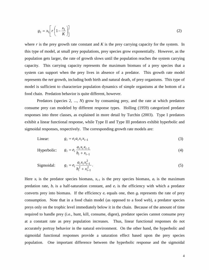
At the lowest level of the food chain (species 1), simple prey species are typically

modeled as growing either exponentially or logistically in the absence of a predator. Logistic

models tend to better represent real systems, as these models account for the effect of prey

density on growth. The logistic growth model is:

4

−=

K

xrxg 1

11 1 (2)

where r is the prey growth rate constant and K is the prey carrying capacity for the system. In

this type of model, at small prey populations, prey species grow exponentially. However, as the

population gets larger, the rate of growth slows until the population reaches the system carrying

capacity. This carrying capacity represents the maximum biomass of a prey species that a

system can support when the prey lives in absence of a predator. This growth rate model

represents the net growth, including both birth and natural death, of prey organisms. This type of

model is sufficient to characterize population dynamics of simple organisms at the bottom of a

food chain. Predation behavior is quite different, however.

Predators (species 2, ..., N) grow by consuming prey, and the rate at which predators

consume prey can modeled by different response types. Holling (1959) categorized predator

responses into three classes, as explained in more detail by Turchin (2003). Type I predators

exhibit a linear functional response, while Type II and Type III predators exhibit hyperbolic and

sigmoidal responses, respectively. The corresponding growth rate models are:

Linear: 1−= iiiii xxaeg (3)

Hyperbolic: 1

1

−

−

+=

ii

iiiii xb

xxaeg (4)

Sigmoidal: 21

2

21

−

−

+=

ii

iiiii

xb

xxaeg . (5)

Here xi is the predator species biomass, xi-1 is the prey species biomass, ai is the maximum

predation rate, bi is a half-saturation constant, and ei is the efficiency with which a predator

converts prey into biomass. If the efficiency ei equals one, then gi represents the rate of prey

consumption. Note that in a food chain model (as opposed to a food web), a predator species

preys only on the trophic level immediately below it in the chain. Because of the amount of time

required to handle prey (i.e., hunt, kill, consume, digest), predator species cannot consume prey

at a constant rate as prey population increases. Thus, linear functional responses do not

accurately portray behavior in the natural environment. On the other hand, the hyperbolic and

sigmoidal functional responses provide a saturation effect based upon the prey species

population. One important difference between the hyperbolic response and the sigmoidal

5

response arises as the prey population diminishes towards zero. As the prey population

approaches zero, the rate of change in prey consumption rate modeled by the hyperbolic

response increases, while the rate of change in prey consumption rate modeled by the sigmoidal

model response passes through an inflection point, and then decreases. This means that as prey

population dwindles to a very low level, predators exhibiting a sigmoidal response slow in their

efforts to consume prey, while hyperbolic predators work harder for their meals. This reduction

in effort by sigmoidal predators to catch prey is typical of a generalist predator that switches to

another food source when prey abundance becomes low. The hyperbolic response is

characteristic of specialist predators, which do not alternate food sources. Specialist predation is

generally seen as a more accurate representation of many systems, including aquatic systems;

however, both types of behavior can be used to model natural systems.

The species removal rate generally involves two terms, one accounting for death by

predation, and the other being a density-dependant death rate term accounting for natural death

and other forms of removal (e.g., harvesting, washout, etc.). The loss of biomass by predation at

one trophic level is directly related to the growth by predation at the next highest level in the

food chain, and differs only by the efficiency factor introduced above. Thus, for example, the

removal rate for a species i with a hyperbolic predator (species i+1) would be represented by:

iiii

iiii xd

xb

xxam +

+=

+

++

1

11 (6)

where di is the death rate constant. Note that the form of the first term (removal by predation)

depends on the form of the predator growth rate. Expressions such as this for mi, which include

both the predation term and the density-dependent death rate term, will apply for i = 2, ..., N – 1.

For the bottom prey species (i = 1), there is no density-dependent death rate term as this is

accounted for in the logistic growth rate model. For the top predator species (i = N), there is no

consumption by predation term, since there is no predator higher in the food chain.

Based on the concepts outlined above, one can form a model of a food chain consisting of

any number of species that exhibit a variety of functional responses. For example, consider a

tritrophic (N = 3) chain with a logistic prey (i = 1), and hyperbolic (Holling Type II) predator (i =

2) and superpredator (i = 3) responses:

6

+−

−=

+−

−=

12

2211

12

21211

1 11xb

xa

K

xrx

xb

xxa

K

xrx

dt

dx (7)

−

+−

+=−

+−

+= 2

23

33

12

122222

23

323

12

2122

2 dxb

xa

xb

xaexxd

xb

xxa

xb

xxae

dt

dx (8)

−

+=−

+= 3

23

233333

23

3233

3 dxb

xaexxd

xb

xxae

dt

dx (9)

This model is well-known as a tritrophic Rosenzweig-MacArthur model (also referred to as a

tritrophic Oksanen model), and is frequently used in theoretical ecology (e.g., Gragnani et al.,

1998; Hastings and Powell, 1991; Klebanoff and Hastings, 1994; Abrams and Roth, 1994;

Kuznetsov and Rinaldi, 1996; De Feo and Rinaldi, 1997). Since this model is relatively simple

and has been widely studied both analytically and numerically, it provides a good initial problem

for testing the feasibility of the interval-based methodology described below for determining

equilibrium states and bifurcations of equilibria in food chain models.

Two additional tritrophic models, involving different predator functional responses, will

be used as test problems. The first of these involves a sigmoidal (Holling Type III) predator and

superpredator, and is given by:

+−

−=

21

22

21211

1 1xb

xxa

K

xrx

dt

dx (10)

−

+−

+= 22

223

32321

22

212

222 d

xb

xxa

xb

xaex

dt

dx (11)

−

+= 32

223

223

333 d

xb

xaex

dt

dx (12)

This model appears to have received only limited study (Turchin, 2003; Yodzis, 1989), as the

Type III functional response is generally only applicable to generalist, not specialist, predators,

and is thus perhaps less widely applicable in typical natural environments than the Rosenzweig-

MacArthur model.

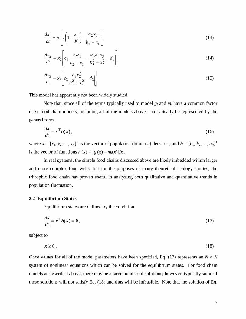
The second of the two additional test problems involves a hyperbolic, or specialist,

predator and a sigmoidal, or generalist, superpredator. This model is given by:

7

+−

−=

12

2211

1 1xb

xa

K

xrx

dt

dx (13)

−

+−

+= 22

223

323

12

1222

2 dxb

xxa

xb

xaex

dt

dx (14)

−

+= 32

223

223

333 d

xb

xaex

dt

dx (15)

This model has apparently not been widely studied.

Note that, since all of the terms typically used to model gi and mi have a common factor

of xi, food chain models, including all of the models above, can typically be represented by the

general form

)(T xhxx=

dt

d, (16)

where x = [x1, x2, ..., xN]T is the vector of population (biomass) densities, and h = [h1, h2, ..., hN]T

is the vector of functions hi(x) = [gi(x) – mi(x)]/xi.

In real systems, the simple food chains discussed above are likely imbedded within larger

and more complex food webs, but for the purposes of many theoretical ecology studies, the

tritrophic food chain has proven useful in analyzing both qualitative and quantitative trends in

population fluctuation.

2.2 Equilibrium States

Equilibrium states are defined by the condition

0== )(T xhxx

dt

d, (17)

subject to

0≥x . (18)

Once values for all of the model parameters have been specified, Eq. (17) represents an N × N

system of nonlinear equations which can be solved for the equilibrium states. For food chain

models as described above, there may be a large number of solutions; however, typically some of

these solutions will not satisfy Eq. (18) and thus will be infeasible. Note that the solution of Eq.

8

(17) can be thought of as consisting of 2N subproblems, one for the case of all nonzero xi and

requiring the solution of h(x) = 0, and 2N –1 subproblems corresponding to different

combinations of xi set to zero, each combination requiring the solution of a system hi = 0, i ∈ S,

where S indicates the set of indices corresponding to nonzero xi. In general, each of the

subproblems that must be solved (except for the case x = 0) may have multiple solutions or no

solutions, and so the total number of equilibrium states may be unknown a priori. For simple

models, it may be possible to solve for many of the equilibrium states analytically, but for more

complex models a computational method is needed that is capable of finding, with certainty, all

the solutions of a nonlinear equation system. The interval-Newton procedure described below is

tested here for this purpose. It is applied directly to the solution of Eq. (17) rather than to any of

the several subproblems.

The stability of an equilibrium state can be determined by evaluating the Jacobian matrix

at this state and then examining its eigenvalues. From Eq. (17), the Jacobian matrix J of interest

has the elements

k

iiik x

hxJ

∂

∂=

)(. (19)

According to linear stability analysis, for an equilibrium state to be stable, all of the eigenvalues

of the Jacobian must have negative real parts.

Examining equilibrium states can give us information on how the behavior of the system

changes with changes in the model parameters. Since the parameters in the model are

representative of physical and biological characteristics of the system, the model parameters can

be altered in order to represent changes in a real system. Tracking the changes in the equilibrium

states can give us information on how a real system might behave when undergoing

perturbations in the system parameters.

2.3 Codimension-One Bifurcations

To find bifurcations of codimension one, all model parameters but one are specified, and

then the values of the remaining parameter at which there is a sudden change in the nature of an

equilibrium state are found. Of interest here are fold and transcritical bifurcations of equilibria

and Hopf bifurcations. Mathematically, when an equilibrium state undergoes either a fold or a

transcritical bifurcation, an eigenvalue of its Jacobian becomes zero. In this case, there are two

9

equilibria that “collide” as the free parameter is varied. In a fold bifurcation, these equilibria

mutually annihilate, thus the number of equilibrium states changes by two as the free parameter

is increased or decreased. On the other hand, in a transcritical bifurcation, the two colliding

equilibria do not disappear, but may simply exchange stability. In a system with a single state

variable, there will always be an exchange of stability, but if the number of state variables is

more than one, there may or may not be an exchange of stability, depending on the sign of the

other eigenvalues. Mathematically, a Hopf bifurcation occurs when its Jacobian has a pair of

complex conjugate eigenvalues and the sign of their real part changes; i.e. when this complex

conjugate pair of eigenvalues is purely imaginary. In a system with two state variables, this will

result in a change in the stability of the equilibrium state, but if the number of state variables is

more than two, there may or may not be stability change, depending on the sign of the other

eigenvalues. If the Hopf bifurcation occurs in an independent two-variable subset of state space,

this is referred to as a planar Hopf bifurcation.

The locations of these bifurcations can be computed by solving a nonlinear equation

system that includes the equilibrium conditions, Eq. (17), together with an augmenting (or test)

function that represents the mathematical condition for the type of bifurcation sought.

Kuznetsov (1998) discusses in detail the development of such test functions for the types of

bifurcations of interest here. Generally these test functions are designed to avoid the need for

direct computation of eigenvalues.

At a fold or transcritical bifurcation, an eigenvalue of J is zero. Since the determinant of

a matrix is equal to the product of its eigenvalues, the determinant of J will be zero at a fold or

transcritical bifurcation, thereby providing a convenient test function. Thus, to locate a fold or

transcritical bifurcation of equilibrium, a nonlinear equation system that can be solved is

0=),(T αxhx (20)

0)],(det[ =αxJ (21)

This is a system of N + 1 equations in the N + 1 variables x and α, where α is the free model

parameter.

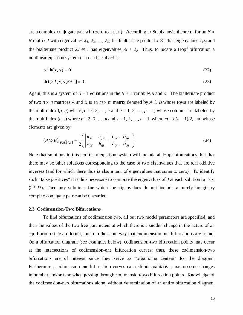
At a Hopf bifurcation, J has a complex conjugate pair of purely imaginary eigenvalues.

This means that there must be a pair of eigenvalues that sums to zero (but note that the converse

is not true—having a pair of eigenvalues that sums to zero does not necessarily mean that they

10

are a complex conjugate pair with zero real part). According to Stephanos’s theorem, for an N ×

N matrix J with eigenvalues λ1, λ2, …, λN, the bialternate product J ⊗ J has eigenvalues λiλj and

the bialternate product 2J ⊗ I has eigenvalues λi + λj. Thus, to locate a Hopf bifurcation a

nonlinear equation system that can be solved is

0=),(T αxhx (22)

0]),(2det[ =⊗ IJ αx . (23)

Again, this is a system of N + 1 equations in the N + 1 variables x and α. The bialternate product

of two n × n matrices A and B is an m × m matrix denoted by A ⊗ B whose rows are labeled by

the multiindex (p, q) where p = 2, 3, …, n and q = 1, 2, …, p – 1, whose columns are labeled by

the multiindex (r, s) where r = 2, 3, …, n and s = 1, 2, …, r – 1, where m = n(n – 1)/2, and whose

elements are given by

( )( )( )

+=⊗

qsqr

pspr

qsqr

psprsrqp aa

bb

bb

aaBA

2

1,, . (24)

Note that solutions to this nonlinear equation system will include all Hopf bifurcations, but that

there may be other solutions corresponding to the case of two eigenvalues that are real additive

inverses (and for which there thus is also a pair of eigenvalues that sums to zero). To identify

such “false positives” it is thus necessary to compute the eigenvalues of J at each solution to Eqs.

(22-23). Then any solutions for which the eigenvalues do not include a purely imaginary

complex conjugate pair can be discarded.

2.3 Codimension-Two Bifurcations

To find bifurcations of codimension two, all but two model parameters are specified, and

then the values of the two free parameters at which there is a sudden change in the nature of an

equilibrium state are found, much in the same way that codimension-one bifurcations are found.

On a bifurcation diagram (see examples below), codimension-two bifurcation points may occur

at the intersections of codimension-one bifurcation curves; thus, these codimension-two

bifurcations are of interest since they serve as “organizing centers” for the diagram.

Furthermore, codimension-one bifurcation curves can exhibit qualitative, macroscopic changes

in number and/or type when passing through codimension-two bifurcation points. Knowledge of

the codimension-two bifurcations alone, without determination of an entire bifurcation diagram,

11

can be useful for comparison of models (Gragnani et al., 1998).

Corresponding to the types of codimension-one bifurcations considered here, there are

three basic types of codimension-two bifurcations. They can be classified mathematically by

examining the eigenvalues of the unaugmented Jacobian J defined by Eq. (19). The Jacobian

can either have a pair of purely zero eigenvalues (double-fold or double-zero bifurcation), two

pairs of purely imaginary complex conjugate eigenvalues (double-Hopf bifurcation), or a pair of

purely imaginary complex conjugate eigenvalues and one zero eigenvalue (fold-Hopf

bifurcation). Since the examples used in this paper are tritrophic, the double-Hopf case will not

be considered here, as these cannot occur in a model with less than four equations (the double-

Hopf condition involves four eigenvalues). There are also other types of codimension-two

bifurcations (e.g., cusp bifurcation) that are not searched for directly here, but which may be

encountered (see Section 4.2).

Both double-fold and fold-Hopf bifurcations can be found be solving the doubly

augmented nonlinear system

0=),,(T βαxhx (25)

0)],,(det[ =βαxJ (26)

0]),,(2det[ =⊗ IJ βαx . (27)

This is a system of N + 2 equations in the N + 2 variables x, α, and β, where α and β are the free

model parameters. Eq. (26) applies since, at either a double-fold or fold-Hopf bifurcation, J

must have an eigenvalue of zero. Eq. (27) applies since, whether it is the pair of zero

eigenvalues at a double-fold bifurcation or the pair of purely imaginary complex conjugate

eigenvalues at a fold-Hopf bifurcation, J must have a pair of eigenvalues that sums to zero.

Once found, solutions to Eqs. (25-27) must be screened for points that have a pair of (nonzero)

eigenvalues that are purely real additive inverses, and the points must be further sorted and

classified by type. Whether one is looking for fold and transcritical bifurcations and solving Eqs.

(20-21), looking for Hopf bifurcations and solving Eqs. (22-23), or looking for codimension-two

bifurcations by solving Eqs. (25-27), the equation system that must be solved may have multiple

solutions, or no solutions, and the number of solutions may be unknown a priori. A

computational method is needed that is capable of finding, with certainty, all the solutions of

12

these nonlinear equation systems. The interval-Newton procedure described below is tested here

for this purpose.

3. COMPUTATIONAL METHODOLOGY

Recent monographs that introduce interval mathematics, as well as computations with

intervals, include those of Neumaier (1990), Hansen (1992) and Kearfott (1996). Of particular

interest here is the use of an interval-Newton/generalized-bisection (IN/GB) technique. Properly

implemented, this technique provides the power to find, with mathematical and computational

certainty, narrow enclosures of all solutions of a system of nonlinear equations, or to determine

with certainty that there are none, provided that initial upper and lower bounds are available for

all variables (Neumaier, 1990; Hansen, 1992, Kearfott, 1996). This is made possible through the

use of the powerful existence and uniqueness test provided by the interval-Newton method. The

key ideas of the methodology used are summarized briefly here.

Consider an n × n nonlinear equation system f(x) = 0 with a finite number of real roots in

some initial interval X(0). The interval Newton methodology is applied to a sequence of

subintervals of X(0). For a subinterval X(k) in the sequence, the first step is the function range

test. An interval extension F(X(k)) of the function f(x) is calculated, which provides upper and

lower bounds on the range of values of f(x) in X(k). Interval extensions are computed here by

substituting the given interval into the function and then evaluating the function using interval

arithmetic. If there is any component of the interval extension F(X(k)) that does not include zero,

then the interval can be discarded, since no solution of f(x) = 0 can exist in this interval. The

next subinterval in the sequence may then be considered. Otherwise, testing of X(k) continues.

The next step is the interval-Newton test. The linear interval equation system

)())(( )()()()( kkkkF xfxNX −=−′ (28)

is solved for a new interval N(k), where F′(X(k)) is an interval extension of the Jacobian of f(x),

and x(k) is an arbitrary point in X(k). It can be shown (Moore, 1966) that any root contained in X(k)

is also contained in the image N(k). This implies that when X(k) ∩ N(k) is empty, then no root

exists in X(k), and also suggests the iteration scheme X(k+1) = X(k) ∩ N(k). In addition, if N(k) ⊂

X(k), it can been shown (e.g., Kearfoot, 1996) that there is a unique root contained in X(k) and thus

in N(k). Thus, after computation of N(k), there are three possibilities: 1. X(k) ∩ N(k) = ∅, meaning

13

there is no root in the current interval X(k) and it can be discarded; 2. N(k) ⊂ X(k), meaning that

there is exactly one root in the current interval X(k). 3. Neither of the above, meaning that no

conclusion can be drawn. In the last case, if X(k) ∩ N(k) is sufficiently smaller than X(k), then the

interval-Newton test can be reapplied to the resulting intersection. Otherwise, the intersection is

bisected, and the resulting two subintervals are added to the sequence of subintervals to be

tested. If an interval containing a unique root has been identified, then this root can be tightly

enclosed by continuing the interval-Newton iteration, which will converge quadratically to a

desired tolerance (on the enclosure diameter). Alternatively, a point approximation of the root

can be found by using a routine point-Newton method, starting from any point in the interval

containing the unique root. This approach is referred to as an interval-Newton/generalized-

bisection (IN/GB) method. At termination, when the subintervals in the sequence have all been

tested, either all the real roots of f(x) = 0 have been tightly enclosed or it is determined

rigorously that no roots exist. Additional details of the IN/GB algorithm used are summarized by

Schnepper and Stadtherr (1996).

An important feature of this approach is that, unlike standard methods for nonlinear

equation solving that require a point initialization, the IN/GB methodology requires only an

initial interval, and this interval can be sufficiently large to enclose all feasible results. In recent

years, the IN/GB technique has been successfully applied to a variety of problems in chemical

engineering, including phase equilibrium (Hua et al., 1998; Maier et al., 1998; Stradi et al.,

2001; Xu et al., 2002), parameter estimation (Gau and Stadtherr, 2000, 2002a,b; Gau et al.,

2000) and density functional theory (Maier and Stadtherr, 2001).

4. RESULTS AND DISCUSSION

In this section, we use the three tritrophic food chain models introduced in section 2.1 as

test problems to explore the use of the IN/GB methodology for computing equilibrium states and

bifurcations of equilibria. It should be noted that, since these are relatively simple models, it is

possible to perform some of these computations analytically. However, since this may not be

possible for more complex models, all the results presented below were computed numerically

using the IN/GB technique, without any analytical short cuts.

14

4.1 Rosenzweig-MacArthur Model

The Rosenzweig-MacArthur model used here is tritrophic, featuring a logistic prey species

and hyperbolic (Holling Type II) predator and superpredator, and defined by Eqs. (7-9). Much

of the literature work on the Rosenzweig-MacArthur model has focused on the enrichment

paradox and chaos associated with alterations of the food chain carrying capacity (e.g., Gragnani

et al., 1998). To conform to these studies and to thus provide a body of work with which to

compare our results, the growth rate constant r and carrying capacity K were chosen as the initial

set of adjustable parameters to study. Following Gragnani et al. (1998), the remaining

parameters values were fixed at a2 = 5/3, b2 = 1/3, e2 = 1, d2 = 0.4, a3 = 0.05, b3 = 0.5, e3 = 1, and

d3 = 0.01. Except as noted otherwise, these parameter values were used for all of the

computations done here with the Rosenzweig-MacArthur model, as well as with the other two

tritrophic models used.

4.1.1 Equilibrium States

As an initial test of the IN/GB methodology, we used it to compute equilibrium states for

several sets of K and r values. For example consider the case of K = 1.0 and r = 1.0. With these

values of K and r, together with the other parameter values given above, the IN/GB method was

used to solve Eq. (17) for all equilibrium states. The initial interval used for each variable was

[0, 5000]; here the upper bound is simply an arbitrarily large number. The results are shown in

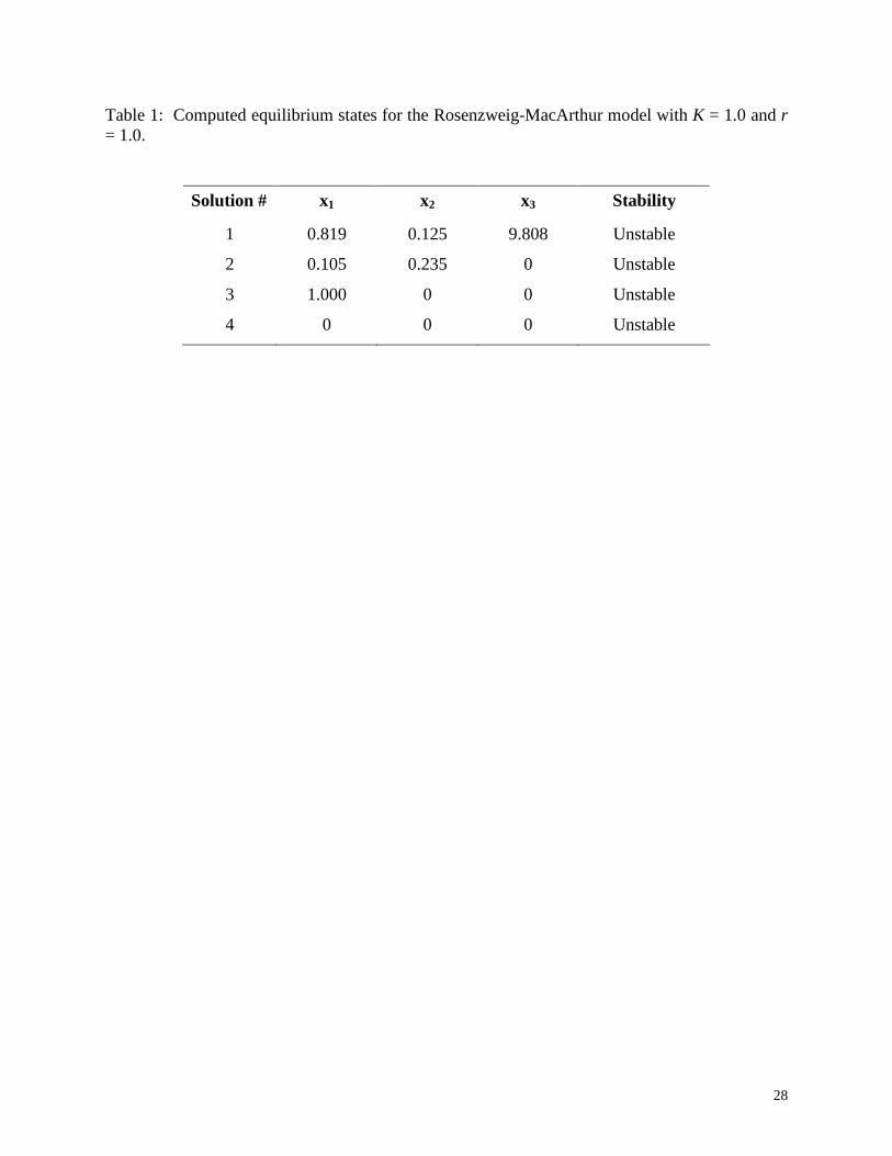
Table 1, along with results of stability analysis for each point. Four feasible steady states were

found, all of which are unstable. Note that the values of x reported in Table 1 (as well as in

Table 2 below) are rounded point representations of the interval enclosures determined by the

IN/GB algorithm. For instance, the actual results computed for the first equilibrium state are the

enclosures x1 ∈ [0.819245918, 0.819246099], x2 ∈ [0.124999908, 0.125000008] and x3 ∈

[9.808198838, 9.808199175]. Tighter enclosures can be determined if desired by setting a

smaller tolerance for the enclosure diameter.

As another example, consider the case of K = 0.5 and r = 1.0. Results for this case are

listed in Table 2. Again there are four feasible equilibrium states, with one stable state in this

case. Both cases considered feature a steady-state with all species coexisting, along with a state

including the prey and predator only, a state including the prey only, and a state for which all

populations are zero. A zero population solution (solution 4) is always unstable. Physically, this

15

means that the populations in any closed system whose initial populations are zero will remain

zero. However, if the system is open and there is a small perturbation (increase) in the prey

population, then the prey population will grow according to the logistic growth rate term until a

new steady state is reached (solution 3). Such perturbations are common in aquatic

environments due to flow and drift.

For a given set of K and r values, the computation of the equilibrium states using IN/GB

is quite fast. Computation times are on the order of 0.05 sec. All computation times given here

and below are for a Dell workstation running a 1.7 GHz Intel Xeon processor and using the Intel

Fortran Compiler 7.1 for Linux.

4.1.2 Solution Branch Diagrams

By comparing the two cases considered above, it can be seen that an effect of increasing

K from 0.5 to 1.0 is that the coexistence equilibrium state goes from stable to unstable. To see

the changes in the equilibrium states as one parameter is varied, solution branch diagrams can be

used. These are plots of both the stable and unstable steady states versus one of the parameters.

Figure 1 shows the solution branch diagrams for the Rosenzweig-MacArthur model as K is

varied with r = 1.0. These diagrams were generated by using the IN/GB method to repeatedly

solve Eq. (17) for slightly different values of K, going from K = 0 to K = 2 in steps of ∆K =

0.001, then analyzing the stability of each solution and plotting the results (thick lines represent

stable equilibria, while thin lines represent unstable equilibria). One should note that such

diagrams do not give the user any information on the transient behavior of the system beyond

knowledge of the stability of the equilibrium states.

Examination of Figure 1 shows that as K increases there are three values of K at which

macroscopic changes in the system behavior (bifurcations) occur. The first of these is at K ≈

0.105. Here a new steady state appears (this is evident in the x1 and x2 diagrams only, as the new

steady state has x3 = 0). This is a transcritical bifurcation. In general, at a transcritical

bifurcation there will be two equilibrium states that collide. However, in this case, one of the

colliding states is infeasible and so does not appear on the solution branch diagram. There is

another similar transcritical bifurcation at K ≈ 0.201. Finally at K ≈ 0.768, one of the

equilibrium states (the one with all species coexisting) changes from stable to unstable. This is a

Hopf bifurcation.

16

Figure 1 also illustrates the paradox of enrichment as discussed by Gragnani et al. (1998),

among others. This paradox states that enriching the bottom level of a food chain in order to

increase the population of the top level species may, in fact, result in the decimation of the

species that are wanted in greater abundance. In this case, enrichment of the food chain is

modeled by increasing the prey carrying capacity K. The plot of superpredator population x3 in

Figure 1 illustrates that enriching the food chain results an increase in superpredator population,

but this is stable only to a point. By increasing the carrying capacity beyond this critical point,

the stable steady-state becomes unstable and enrichment may become counterproductive.

Solution branch diagrams such as Figure 1 can be very easily and automatically generated using

the IN/GB methodology, with certainty that all equilibrium states (solution branches) have been

found. Two other solution branch diagrams were computed. Figure 2 shows the case for r = 0.5,

and Figure 3 for r = 0.4.

Figure 2 illustrates some bifurcation behavior similar to Figure 1, but with distinct

differences. Here as K is increased, the system undergoes a transcritical bifurcation in which a

previously infeasible equilibrium state becomes feasible, colliding with another equilibrium state

and exchanging stabilities. This is followed by a Hopf bifurcation, which occurs for an

equilibrium state with a positive prey and predator population, but with a zero superpredator

population. Therefore, this is a planar Hopf bifurcation, as the bifurcation is occurring in a

subset of the state space of the model. At K ≈ 0.872, a fold bifurcation occurs and two new

steady states appear (this is evident only in the plots of x1 and x3, as the new steady states have

the same value of x2). Finally there are two Hopf bifurcations. One can observe that there is no

continuity between the equilibrium that undergoes the first (planar) Hopf bifurcation and the

equilibrium that undergoes the second two (non-planar) Hopf bifurcations. From the plot of x3, it

is evident that the region of stable coexistence of all three populations at equilibrium is in the

narrow interval of K values between the second two Hopf bifurcation points. However, in this

region, the trend of the enrichment paradox is apparent.

Looking at Figure 3, one can see that the slight change made in the prey growth rate

constant r leads to a significant change in system behavior. The narrow band of stability in

Figure 2 that allows all three species to coexist no longer exists in Figure 3. Thus, at a

sufficiently low prey growth rate, no superpredators can thrive in a stable population. It is also

very interesting to note that in Figure 3 the fold bifurcation results in two equilibrium states

17

(solution branches) that do not intersect other branches (this is true even for larger values of K

than shown on the plot). Such isolated solution branches (isola) can be very difficult to find

using continuation methods, especially for more complex models in which their existence may

not be suspected. However, using the IN/GB approach, isolated branches are easily found. In

fact, there is a mathematical and computational guarantee that they will be found.

4.1.3 K vs. r Bifurcation Diagram

For fixed r, the values of K and x at which the bifurcations of equilibria observed above

occur can be computed directly by solving the appropriate augmented systems, namely Eqs. (20-

21) for fold and transcritical bifurcations and Eqs. (22-23) for Hopf bifurcations. In a K vs. r

bifurcation diagram the values of K at which the bifurcations occur are plotted as a function of r.

Such a diagram was generated here by using the IN/GB method to repeatedly solve the

augmented systems for K and x for slightly different values of r, going from r = 0 to r = 2 in

steps of ∆r = 0.005. There may be some values of r for which one of the augmented systems has

an infinite number of solutions for K (i.e., a vertical line on the K vs. r diagram). This case

cannot be handled directly by the IN/GB technique, or could be missed entirely by the stepping

in r. Thus, to ensure that all of the bifurcations are found, it is necessary to also scan in the K

direction. That is, the IN/GB method was also used to repeatedly solve the augmented systems

for r and x for slightly different values of K, in this case going from K = 0 to K = 2 in steps of ∆K

= 0.005. To locate codimension-two bifurcations (double-fold and fold-Hopf), the IN/GB

method was used to solve the doubly augmented system given by Eqs. (25-27) for K, r and x.

The initial intervals used for the components of x were again [0, 5000] and for the parameters K

and r were [0, 2]. The average CPU time for each solution of Eqs. (20-21) for fold and

transcritical bifurcations was about 0.6 seconds, and for each solution of Eqs. (22-23) for Hopf

bifurcations was about 1.4 seconds. Solving Eqs. (25-27) for codimension-two bifurcations

required about 39 seconds.

Figure 4 shows the K vs. r bifurcation diagram generated for the Rosenzweig-MacArthur

tritrophic food chain model using the IN/GB method. Fold and transcritical of equilibria curves

were both found, and are labeled FE and TE respectively. Hopf bifurcation curves were also

found, and are labeled H or Hp (for planar Hopf). A single fold-Hopf bifurcation was located;

this point is represented as an open diamond and labeled FH (no double-fold bifurcations were

18

found). This bifurcation diagram corresponds exactly with the known K vs. r bifurcation

diagram for this model, as reported by Gragnani et al. (1998). This confirms the utility and

accuracy of the IN/GB algorithm for computing bifurcation of equilibria diagrams. Bifurcation

diagrams such as Figure 4 can be very easily and automatically generated using the IN/GB

methodology, with complete certainty that all bifurcation curves have been found. Two other

bifurcation diagrams were computed, d2 vs. K and r vs. d2.

4.1.4 d2 vs. K Bifurcation Diagram

Using the same procedure as described above, a d2 vs. K bifurcation diagram for the

Rosenzweig-MacArthur model was generated. The predator death rate constant d2 is now a free

parameter, and r is now a fixed parameter set at r = 1. The average CPU time for each solution

of Eqs. (20-21) for fold and transcritical bifurcations was about 0.8 seconds, and for each

solution of Eqs. (22-23) for Hopf bifurcations was about 2.1 seconds. Solving Eqs. (25-27) for

codimension-two bifurcations required about 31 seconds. The resulting bifurcation diagram is

shown in Figure 5. This diagram illustrates that at a constant prey carrying capacity and growth

rate constant (r = 1), increasing or decreasing the predator death rate will cause macroscopic

changes in system behavior. For relatively small values of K, there are two transcritical

bifurcations that occur as d2 is changed, and for larger values of K there are also two Hopf

bifurcations. No double-fold or fold-Hopf codimension-two bifurcations were found. In order to

more closely observe these changes in behavior, solution branch diagrams were generated using

IN/GB for the case of K = 1. Figure 6 gives the solution branch diagrams for x as d2 is varied

from 0 to 2.

Based on the bifurcation diagram at K = 1, we would expect that as d2 is increased from 0

to 2, there should be observed first a Hopf bifurcation (the planar Hopf is not observed in this

case, due to the sign of the third eigenvalue) and then two transcritical bifurcations. This is what

is in fact seen in Figure 6. These diagrams illustrate that there is a minimum predator death rate

constant d2 that results in stable system behavior. At low predator death rates, the system is

unstable and likely exhibits cycles of population booms and busts. As the predator death rate

increases, enough predators are dying off at any given time to prevent the cycles from occurring,

and the cycles collapse to a stable steady-state in a Hopf bifurcation.

These results also give a sense of the effects of releasing a toxin that specifically targets

the predator trophic level, and increases the predator death rate constant. Prior to examining

19

these diagrams, one would expect that such a release would have an impact on both the predator

and the superpredator populations. The plot of x3 in Figure 6 shows that increasing the predator

death rate constant causes a linear decrease in the stable superpredator biomass. However,

according to the plot of x2 in Figure 6, the stable predator population is not affected until the

superpredator population reaches zero. Though these results may seem somewhat

counterintuitive, they are indicative of the complex interactions that may occur in food chains.

An ecotoxin released at a very low concentration could affect organisms at different trophic

levels to varying degrees. For the case considered here, one might observe an impact on the

superpredator population and thus assume that the effect of the ecotoxin was at that level, even

though the actual impact is on the predator level. Using models such as this one can obtain

insights into the impacts of an ecotoxin that might not otherwise be apparent.

4.1.5 r vs. d2 Bifurcation Diagram

Again using the IN/GB methodology, an r vs. d2 bifurcation diagram for the Rosenzweig-

MacArthur model was generated, with K fixed at K = 1. This set of free parameters is of interest

since both could be affected by an ecotoxin. Since the prey growth rate constant represents the

net growth (accounting for both birth and natural death), an ecotoxin affecting the prey trophic

level could decrease the prey growth rate. For this problem, the average CPU time for each

solution of Eqs. (20-21) for fold and transcritical bifurcations was about 2.4 seconds, and for

each solution of Eqs. (22-23) for Hopf bifurcations was about 2.2 seconds. Solving Eqs. (25-27)

for codimension-two bifurcations required about 220 seconds. The resulting bifurcation diagram

is shown in Figure 7.

Figure 7 displays a wide variety of bifurcation behavior, including a codimension-two

fold-Hopf bifurcation. This diagram illustrates that changing either the prey growth rate constant

or the predator death rate constant can cause macroscopic changes in system behavior. Two

solution branch diagrams were generated in IN/GB to more closely examine the changes in

species biomass as the parameter variables are changed. Figure 8 is the solution branch diagram

as d2 is changed at a constant r = 0.5, and Figure 9 is the solution branch diagram as r is changed

at a constant d2 = 0.4.

The solution branch diagrams in Figure 8 (r = 0.5; K = 1.0) illustrate behavior somewhat

similar to the solution branch diagrams illustrated in Figure 6 (r = 1.0; K = 1.0), with important

differences. First, in Figure 8 a third transcritical bifurcation is observed, at a value of d2 very

20

close to the Hopf bifurcation. Also, compared to Figure 6, the Hopf bifurcation now occurs at a

lower value of d2, as does the point where the system can no longer support superpredators and

they become extinct. However, the point at which the predator population becomes extinct does

not change, nor does the rate of superpredator decline. Therefore, with a decrease in the prey

growth rate constant from r = 1.0 to r = 0.5, the system actually has a wider range of d2 that

results in a stable system, and a wider range of d2 in which all three species can coexist.

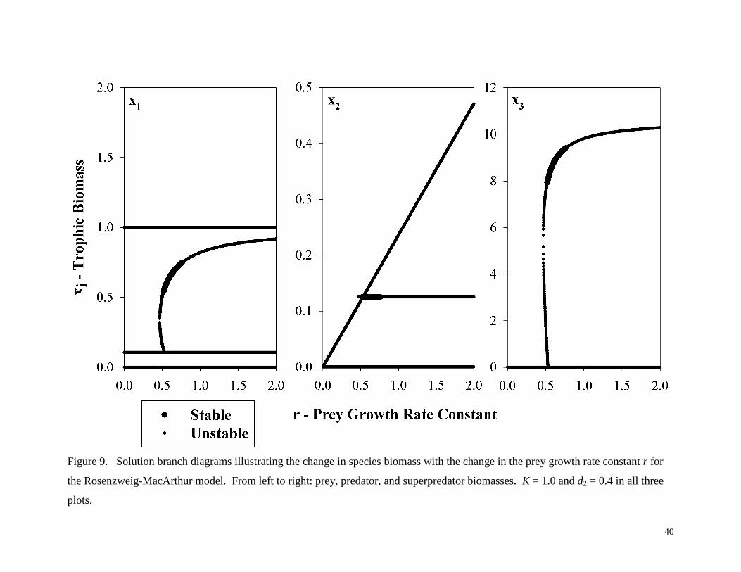
Figure 9 illustrates the effect of increasing the prey growth rate constant on a system with

constant carrying capacity K = 1.0 and constant predator death rate constant d2 = 0.4. These

solution branch diagrams tie together Figure 4 (K vs. r at constant d2 = 0.4) and Figure 7 (r vs. d2

at constant K =1.0) in that they are evaluated at a parameter set (K = 1.0; d2 = 0.4) common to

both diagrams. As r increases, the solution branch diagrams illustrated in Figure 9 exhibit a fold

bifurcation, then a Hopf bifurcation, followed very closely by a transcritical bifurcation, and

finally another Hopf bifurcation. The location of these bifurcations can be verified by both

Figure 4 (following the line K = 1 upwards) and Figure 7 (following the line d2 = 0.4 upwards).

This example and those above are useful in confirming that the IN/GB methodology is indeed

successfully computing all equilibrium states and bifurcations of equilibria for this model. The

solution branch diagrams of Figure 9 show a single region of stability for the model, and in this

region all three species coexist. In this region, increasing the prey growth rate constant causes an

increase in prey and superpredator population, but this occurs only to a point. This type of

phenomenon is similar to the paradox of enrichment. As the prey species replaces its population

more quickly, more organisms are able to thrive within the food chain, but eventually if the prey

population grows too quickly, the system becomes unstable.

4.2 Tritrophic Model with Sigmoidal Predator and Superpredator Responses

In view of the success in applying the IN/GB methodology to generate bifurcation

diagrams and solution branch diagrams for the Rosenzweig-MacArthur model, the methodology

was tested on two other food chain models. The first of these is the tritrophic model with

sigmoidal (Holling Type III) predator and superpredator functional responses, as given by Eqs

(10-12).

21

4.2.1 Bifurcation Diagram

The dynamics of this system have received only limited study (Turchin, 2003; Yodzis,

1989), and there are apparently no published bifurcation diagrams for it. Following the

procedures outlined above, the IN/GB methodology was applied to compute the bifurcation

diagram for the case of r and K as free parameters. The average CPU time for each solution of

Eqs. (20-21) for fold and transcritical bifurcations was about 3.6 seconds, and for each solution

of Eqs. (22-23) for Hopf bifurcations was about 7.9 seconds. Solving Eqs. (25-27) for

codimension-two bifurcations (double-fold or fold-Hold) required about 71 seconds. The

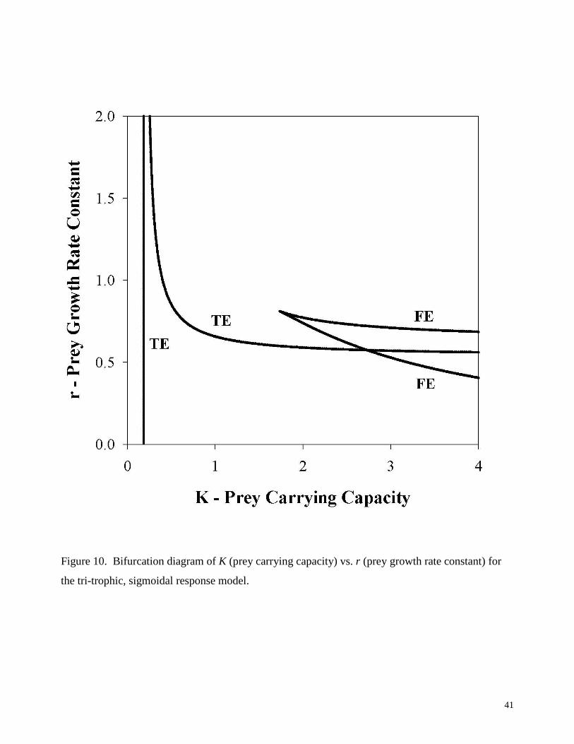
resulting bifurcation diagram is shown in Figure 10.

At least for the range of parameters studied, no Hopf bifurcations were found, and no

double-fold or fold-Hopf codimension-two bifurcations were found. Note that the range of prey

carrying capacity values studied was increased to [0, 4] in order to more closely examine the pair

of fold of equilibria curves discovered. These curves are isolated from the transcritical of

equilibria bifurcation curves in the parameter-state space in which Eqs. (20-21) are solved, and

so could be difficult to detect using continuation methods. The intersection of the two fold of

equilibria bifurcation curves without the occurrence of a double-fold bifurcation suggests that

this point is a cusp bifurcation. Note that this type of codimension-two bifurcation cannot be

found by solving Eqs. (25-27). In order to investigate the behavior of the system near the cusp,

solution branch diagrams were generated for the case r = 0.7 using the IN/GB methodology.


A set of solution branch diagrams was generated for this model that examines the effect

of increasing the prey carrying capacity K on the biomasses of the three trophic levels while

holding r constant at a value of 0.7. This value was chosen to intersect with the fold bifurcation

curves close to the cusp. Figure 11 gives the solution branch diagrams. These illustrate the

crossing of two transcritical bifurcations followed by two fold bifurcations. One equilibrium

created by the first fold bifurcation collides with the equilibrium that appears in the second

transcritical bifurcation and the two mutually annihilate in the second fold bifurcation, forming

an S shaped curve typical of behavior near a cusp bifurcation. Note that there is a region where

two stable steady-states exist in which all three species can coexist; this region also contains an

unstable-steady state (this is not seen in the plot for x2 since all three of these solutions have the

22

same x2 value). It also appears, according to this model, that the enrichment paradox does not

hold for systems of generalist predators, as increasing K does not ultimately result in an unstable

system. However, it should be noted that in this system the two fold bifurcations are catastrophic

because they result in an abrupt change in system behavior. For instance, if the system is at the

stable high-population (prey and superpredator) equilibrium state, and the prey carrying capacity

K is decreasing, then, at the leftmost fold bifurcation, this state suddenly disappears and is

replaced by a low-population equilibrium state. The transient behavior by which the new low-

population state is approached is not investigated here.

4.3 Tritrophic Model with Hyperbolic Predator and Sigmoidal Superpredator Responses

The last of the food chain models used as a test problem here is the tritrophic model with

a hyperbolic (Holling Type II) predator response and a sigmoidal (Holling Type III)

superpredator response, as given by Eqs (13-15).

4.3.1 Bifurcation Diagram

This model has apparently received little, if any, previous study. Using a hyperbolic

(specialist) predator and a sigmoidal (generalist) superpredator is justifiable in that organisms

that are higher up on a food chain tend to have more diversity in the types of organisms that

compose their diets. Again the IN/GB methodology was applied to compute the bifurcation

diagram for the case of r and K as free parameters. The average CPU time for each solution of

Eqs. (20-21) for fold and transcritical bifurcations was about 2.1 seconds, and for each solution

of Eqs. (22-23) for Hopf bifurcations was about 3.8 seconds. Solving Eqs. (25-27) for

codimension-two bifurcations (double-fold or fold-Hold) required about 62 seconds. The

resulting bifurcation diagram is shown in Figure 12.

The bifurcation diagram illustrates a range of features, including fold and transcritical of

equilibria bifurcations, Hopf bifurcations, and a codimension-two bifurcation point classified as

a fold-Hopf bifurcation. The fold and transcritical bifurcation curves appear to be quite similar

to those seen in the Rosenzweig-MacArthur model, however the Hopf bifurcation behavior is

quite different in that the Hopf curve that originates at the fold-Hopf bifurcation point does not

double back in the diagram for this model. Also the fold-Hopf point occurs at a significantly

larger value of r.

23


Using the IN/GB methodology, solution branch diagrams were generated for this model

that examine the effect of increasing the prey carrying capacity K on the biomasses in the three

trophic levels, while holding r constant at a value of 1.0. These diagrams are shown in Figure

13. The solution branch diagrams illustrate a transcritical bifurcation followed by a Hopf

bifurcation and then a fold bifurcation. An interesting feature to note is that the Hopf bifurcation

that causes a change in system stability is, in fact, a planar Hopf bifurcation. A second Hopf

bifurcation is encountered with no change in system stability. This Hopf bifurcation is non-

planar, but a change in stability does not occur as the sign of the third eigenvalue is already

positive. As one equilibrium created in the fold bifurcation approaches K = 2.0, it grows close to

a transcritical bifurcation. This model displays a region of instability between the Hopf and fold

bifurcations. However, the model does not exhibit behavior in accordance with the enrichment

paradox. While increasing the prey carrying capacity does take the system through a region of

instability, the presence of a generalist superpredator causes the system to be stable for larger

values of K, at least for the parameter values at which this diagram was generated.

4.4 Computational Performance

Average computation times are given above for single solutions of the appropriate

nonlinear equation systems for determination of equilibrium states, codimension-one bifurcations

and codimension-two bifurcations. To generate an equilibrium solution branch diagram or a

bifurcation diagram requires that these equation systems be solved multiple times. For instance,

a solution branch diagram generated over a parameter range [0, 2] with a step size of 0.001

would require 2000 solutions of Eq. (17) for the equilibrium states. With a solution time on the

order of 0.05 seconds for an individual system, this means that the entire solution branch

diagram requires roughly 100 seconds of computation time. Bifurcation diagrams are more

costly since both Eqs. (20-21) and Eqs (22-23) must be solved repeatedly, and Eqs. (25-27) once.

For example, the K vs. r bifurcation diagram for the Rosenzwieg-MacArthur model requires

about 1640 seconds of computation time. We do not consider computational effort on this order

to be unreasonable, especially since the methodology used provides a guarantee of reliability.

Furthermore, since the diagrams can be generated automatically, without user intervention to

24

deal with initialization issues, the actual elapsed time to generate a bifurcation diagram for a new

model may actually be significantly less than when initialization-dependent methods are used.

Since all of the nonlinear equation systems that must be solved to generate a diagram are

independent of each other, one obvious way to improve computational performance is to use

parallel computing. Distribution of the independent equation systems across multiple processors

will result in essentially linear speedup. Furthermore, the IN/GB methodology itself can be

readily parallelized; for example, Gau and Stadtherr (2002c) have described an MPI-based

implementation of IN/GB that provides very efficient processor utilization. The serial

performance of the methodology can also be easily improved by using additional tools from

interval analysis, including constraint propagation and the exploitation of function properties

(e.g., monotonicity) in evaluating interval extensions. The work of Maier and Stadtherr (2001)

on an application arising in the modeling of phase transitions in nanopores demonstrates the use

of these types of techniques.

5. CONCLUDING REMARKS

Using several examples drawn from three different tritrophic food chain models, we have

demonstrated a new methodology for computing all equilibrium states and bifurcations of

equilibria (fold, transcritical, Hopf, double-fold and fold-Hopf). This technique is based on

interval analysis, in particular an interval-Newton/generalized bisection (IN/GB) approach.

Using this methodology it was possible to easily and automatically, without any need for

initialization or a priori insight into expected system behavior, generate complete solution

branch diagrams and bifurcation diagrams. Furthermore, this could be done with certainty, since

the technique provides a mathematical and computational guarantee that all solutions to a system

of nonlinear equations are enclosed. Since this technique is essentially initialization

independent, it can provide a powerful alternative to traditional continuation methods, which in

general are initialization dependant and thus may not be completely reliable. Although the

systems studied here were relatively simple, we anticipate that the methodology used can be

applied to larger and more complex problems, as well as in the analysis of other dynamical

systems of interest in chemical engineering.

25

Acknowledgements

This work was supported in part by the Department of Education Graduate Assistance in

Areas of National Needs (GAANN) Program under Grant #P200A010448, and by the State of

Indiana 21st Century Research and Technology Fund under Grant #909010455. Additional

support has been provided by a University of Notre Dame Schmitt Fellowship (CRG) and by a

University of Notre Dame Center for Applied Mathematics Undergraduate Summer Fellowship

(MPS).

References

Abrams, P. A., & Roth, J. D. (1994). The effects of enrichment of three-species food chains with

non-linear functional responses. Ecology 75, 1118–1130.

Brennecke, J. F., & Maginn, E. J. (2001). Ionic liquids: Innovative fluids for chemical

processing. AIChE Journal 47, 2384-2389.

De Feo, O., & Rinaldi, S. (1997). Yield and dynamics of tritrophic food chains. American

Naturalist 150, 328–345.

Doedel, E. J., Champneys, A. R., Fairgrieve, T. F., Kuznetsov, Y. A., Sandstede, B. and X.J

Wang (1997). AUTO97: Continuation and bifurcation software for ordinary differential

equations. Department of Computer Science, Concordia University, Montreal, Canada

(see also http://indy.cs.concordia.ca/auto/bib)

Freemantle, M. (2002). Meeting briefs: Ionic liquids separated from mixtures by CO2.

Chemical & Engineering News 80 (36), 44-45.

Gau, C.-Y., & Stadtherr, M. A. (2000). Reliable nonlinear parameter estimation using interval

analysis: Error-in-variables approach. Computers & Chemical Engineering 24, 631-638.

Gau, C.-Y., & Stadtherr, M. A. (2002a). Deterministic global optimization for error-in-variables

parameter estimation. AIChE Journal 48, 1192-1197.

Gau, C.-Y., & Stadtherr, M. A. (2002b). Deterministic global optimization for data

reconciliation and parameter estimation using error-in-variables approach. In Recent

Developments in Optimization and Optimal Control in Chemical Engineering (ed. R.

Luus), Transworld Research, pp. 1-17.

26

Gau, C.-Y., & Stadtherr, M. A. (2002c). Dynamic load balancing for parallel interval-Newton

using message passing. Computers & Chemical Engineering 26, 811-825.

Gau, C.-Y., Brennecke, J. F., & Stadtherr, M. A. (2000). Reliable nonlinear parameter estimation

in VLE modeling. Fluid Phase Equilibr., 168 (1): 1-18.

Gragnani, A., De Feo, O., & Rinaldi, S., (1998). Food chains in the chemostat: Relationships

between mean yield and complex dynamics. Bulletin of Mathematical Biology 60, 703-

719.

Hansen, E. R. (1992). Global Optimization Using Interval Analysis, Marcel Dekker, New York.

Hastings, A., & Powell, T. (1991). Chaos in a three-species food chain. Ecology 72, 896-903.

Hua, J. Z., Brennecke, J. F., & Stadtherr, M. A. (1998). Enhanced interval analysis for phase

stability: Cubic equation of state models. Industrial & Engineering Chemistry Research

37, 1519-1527.

Holling, C. S. (1959). Some characteristics of simple types of predation and parasitism.

Canadian Entomologist 91, 385-398.

Kearfott, R. B. (1996). Rigorous Global Search: Continuous Problems, Kluwer, Dordrecht, The

Netherlands.

Klebanoff, A., & Hastings, A. (1994). Chaos in three-species food chains. Journal of

Mathematical Biology 32, 427-451.

Kuznetsov, Y. A. (1998). Elements of Applied Bifurcation Theory, Springer-Verlag, New York.

Kuznetsov, Y. A., & Rinaldi, S. (1996). Remarks on food chain dynamics. Mathematical

Biosciences 134, 1–33.

Jastorff, B., Störmann, R., Ranke, J., Mölter, K., Stock, F., Oberheitmann, B., Hoffmann, W.,

Hoffmann, J., Nüchter, M., Ondruschka, B., & Filser, J. (2003). How hazardous are ionic

liquids? Structure-activity relationships and biological testing as important elements for

sustainability evaluation. Green Chemistry 5, 136-142.

Maier, R.W., & Stadtherr, M. A. (2001). Reliable density-functional-theory calculations of

adsorption in nanoscale pores. AIChE Journal 47, 1874-1884.

Maier, R.W., Brennecke, J. F., & Stadtherr, M. A. (1998). Reliable computation of

homogeneous azeotropes. AIChE Journal 44, 1745-1755.

Moghadas, S. M., & Gumel, A. B. (2003). Dynamical and numerical analyses of a generalized

food-chain model. Applied Mathematics and Computation, 142 (1): 35-49.

27

Moore, R. E. (1966). Interval Analysis, Prentice-Hall, Englewood Cliffs, NJ.

Neumaier, A. (1990). Interval Methods for Systems of Equations, Cambridge Univ. Press,

Cambridge, U.K.

Stradi, B., Brennecke, J. F., Kohn, J. P., & Stadtherr, M. A. (2001). Reliable computation of

mixture critical points. AIChE Journal 47, 212-221.

Turchin, P. (2003). Complex Population Dynamics: A Theoretical/Empirical Synthesis.

Princeton Univ. Press, Princeton, NJ.

van Coller, L. (1997). Automated techniques for the qualitative analysis of ecological models:

Continuous models. Conserv. Ecol. [online], 1 (1), 5. URL:

http://www.consecol.org/vol1/iss1/art5.

Xu, G., Brennecke, J. F., & Stadtherr, M. A. (2002). Reliable computation of phase stability and

equilibrium from the SAFT equation of state. Industrial & Engineering Chemistry

Research 41, 938-952 (2002).

Yodzis, P. (1989). Introduction to Theoretical Ecology. Harper & Row, New York.

28

Table 1: Computed equilibrium states for the Rosenzweig-MacArthur model with K = 1.0 and r = 1.0.

Solution # x1 x2 x3 Stability

1 0.819 0.125 9.808 Unstable

2 0.105 0.235 0 Unstable

3 1.000 0 0 Unstable

4 0 0 0 Unstable

29

Table 2: Computed equilibrium states for the Rosenzweig-MacArthur model with K = 0.5 and r = 1.0.

Solution # x1 x2 x3 Stability

1 0.347 0.125 5.624 Stable

2 0.105 0.208 0 Unstable

3 0.500 0 0 Unstable

4 0 0 0 Unstable

30

List of Figures

Figure 1. Solution branch diagrams illustrating the change in species biomass with the change in

the prey carrying capacity K for the Rosenzweig-MacArthur model. From left to right: prey,

predator, and superpredator biomasses. r = 1.0 for all three plots.







Figure 4. Bifurcation diagram of K (prey carrying capacity) vs. r (prey growth rate constant) for the

Rosenzweig-MacArthur model.

Figure 5. Bifurcation diagram of K (prey carrying capacity) vs. d2 (predator death rate constant) for

the Rosenzweig-MacArthur model. r = 1.0.


the predator death rate constant d2 for the Rosenzweig-MacArthur model. From left to right:

prey, predator, and superpredator biomasses. K = 1.0 and r = 1.0 for all three plots.

Figure 7. Bifurcation diagram of d2 (predator death rate constant) vs. r (prey growth rate constant)

for the Rosenzweig-MacArthur model. K = 1.0.


the predator death rate constant d2 for the Rosenzweig-MacArthur model. From left to right:

prey, predator, and superpredator biomasses. K = 1.0 and r = 0.5 for all three plots.


the prey growth rate constant r for the Rosenzweig-MacArthur model. From left to right:

prey, predator, and superpredator biomasses. K = 1.0 and d2 = 0.4 in all three plots.

Figure 10. Bifurcation diagram of K (prey carrying capacity) vs. r (prey growth rate constant) for

the tri-trophic, sigmoidal response model.


the prey carrying capacity K for the tri-trophic, sigmoidal response model. From left to

right: prey, predator, and superpredator biomasses. r = 0.7 for all three plots.

31


the tri-trophic model with a hyperbolic predator and a sigmoidal superpredator.


the prey carrying capacity K for the tri-trophic model with a hyperbolic predator and a

sigmoidal superpredator. From left to right: prey, predator, and superpredator biomasses. r

= 1.0 for all three plots.

32

Figure 1. Solution branch diagrams illustrating the change in species biomass with the change in the prey carrying capacity K for the

Rosenzweig-MacArthur model. From left to right: prey, predator, and superpredator biomasses. r = 1.0 for all three plots.

33



34



35

Figure 4. Bifurcation diagram of K (prey carrying capacity) vs. r (prey growth rate constant) for the

Rosenzweig-MacArthur model.

36

Figure 5. Bifurcation diagram of K (prey carrying capacity) vs. d2 (predator death rate constant) for

the Rosenzweig-MacArthur model. r = 1.0.

37

Figure 6. Solution branch diagrams illustrating the change in species biomass with the change in the predator death rate constant d2

for the Rosenzweig-MacArthur model. From left to right: prey, predator, and superpredator biomasses. K = 1.0 and r = 1.0 for all

three plots.

38

Figure 7. Bifurcation diagram of d2 (predator death rate constant) vs. r (prey growth rate constant)

for the Rosenzweig-MacArthur model. K = 1.0.

39

Figure 8. Solution branch diagrams illustrating the change in species biomass with the change in the predator death rate constant d2

for the Rosenzweig-MacArthur model. From left to right: prey, predator, and superpredator biomasses. K = 1.0 and r = 0.5 for all

three plots.

40

Figure 9. Solution branch diagrams illustrating the change in species biomass with the change in the prey growth rate constant r for

the Rosenzweig-MacArthur model. From left to right: prey, predator, and superpredator biomasses. K = 1.0 and d2 = 0.4 in all three

plots.

41


the tri-trophic, sigmoidal response model.

42

Figure 11. Solution branch diagrams illustrating the change in species biomass with the change in the prey carrying capacity K for

the tri-trophic, sigmoidal response model. From left to right: prey, predator, and superpredator biomasses. r = 0.7 for all three plots.

43


the tri-trophic model with a hyperbolic predator and a sigmoidal superpredator.

44

Figure 13. Solution branch diagrams illustrating the change in species biomass with the change in the prey carrying capacity K for

the tri-trophic model with a hyperbolic predator and a sigmoidal superpredator. From left to right: prey, predator, and superpredator

biomasses. r = 1.0 for all three plots.

reliable computation of equilibrium states and bifurcations in food

Documents