reliable telecommunication networks
TRANSCRIPT

Budapest University of Technology and Economics (BME)Faculty of Electrical Engineering and Informatics (VIK)
Department of Telecommunications and Media Informatics (TMIT)High-Speed Networks Laboratory (HSNLab)MTA-BME Future Internet Research Group
Reliable Telecommunication Networks
D.Sc. Dissertation
In partial fulfillment of the requirements for the title ofDoctor of the Hungarian Academy of Sciences
Tapolcai Janos, Ph.D.
Magyar tudosok korutja 2., H-1117 Budapest, Hungary,E-mail: [email protected]
Budapest
2012
dc_498_12

ii
dc_498_12

Dedication
This thesis is dedicated to my wife Eszter and my sonMisi. Their patience, love and endurance was essential forfinishing this work.
iii
dc_498_12

iv
dc_498_12

Acknowledgements
This work was carried out at the High-Speed Networks Laboratory (HSNLab) at the De-partment of Telecommunications and Media Informatics (TMIT), Budapest Universityof Technology and Economics (BME) during the years 2005–2012. I am grateful to Pro-fessor Gyula Sallai and Henk Tamas, former and current Heads of the Department, forcontinuously supporting my research during these years.
My deepest gratitude goes to my closest collaborators, Professor Lajos Ronyai (SzTAKI,BME) and Professor Pin-Han Ho (University of Waterloo, Canada), for the mentorship,help, advice and for those many inspiring discussions we had. Lajos’s intellectual prowessis matched only by his genuinely good nature and down-to-earth humility, and I amtruly fortunate to have had the opportunity to work with him. I admire Pin-Han for hisdynamism, enthusiasm, creative ideas and his attitude towards science.
My warmest thanks are due to my office mates and closest co-authors, Gabor Retvariand Peter Babarczi, for those hundreds of hours of discussions and brainstorming wehad in the last five years. I am also grateful to the newly formed Lendulet group withProfessor Jozsef Bıro, Attila Korosi, Andras Gulyas, Zalan Heszberger, Felician Nemethand Balazs Sonkoly. Grateful thanks go to the Phd students I work with, Eva Hosszu, forproofreading the dissertation, and to Mate Nagy and Levente Csikor. I am grateful to allcolleagues of the Lab and of the Department for the nice and inspiring atmosphere.
I wish to express my gratitude to my international collaborators Professor MurielMedard (MIT, USA), Professor Michal Pioro (Warsaw University of Technology, Polandand Lund University, Sweden), Dirk Trossen (Cambridge University, UK), ProfessorKrishnaiyan Thulasiraman (University of Oklahoma, USA), Bin Wu (UESTC, China),Professor Jose L. Marzo (University of Girona, Spain) and Gergely Biczok (NTNU, Nor-way).
I would like to thank my PhD supervisors, Professor Andras Recski and Tibor Cinklerfor starting my research career. I am indebted to Ferenc Nizsalovszki who was my mathteacher at Fazekas Mihaly Secondary School.
Very special thanks go to Ericsson, to MTA Bolyai and Magyary Zoltan PostdoctoralScholarship for financially supporting me and my work during my postdoc research.
Last but not least, I wish to thank my wife Eszter and my son Misi for their love,patience, and endurance to my research-oriented lifestyle. I am grateful to my parents,Laszlo and Irina, for their care, and to my whole family, too. I wish to thank my lovelyfriends for all the fun we had together.
v
dc_498_12

Contents
1 Preface 11.1 Reliable Backbone Networks . . . . . . . . . . . . . . . . . . . . . . . . . . 11.2 Reliable IP Networks . . . . . . . . . . . . . . . . . . . . . . . . . . . . . . 2
2 Failure Localization via a Central Controller 32.1 Introduction . . . . . . . . . . . . . . . . . . . . . . . . . . . . . . . . . . . 3
2.1.1 Categorization of Optical Layer Failure Localization Schemes . . . . 4The Types of Failures . . . . . . . . . . . . . . . . . . . . . . . . . 4The Constraints on the Monitoring Lightpaths . . . . . . . . . . . . 5Failure Localization Time . . . . . . . . . . . . . . . . . . . . . . . 5
2.1.2 Problem Input . . . . . . . . . . . . . . . . . . . . . . . . . . . . . 6Shape Constraints . . . . . . . . . . . . . . . . . . . . . . . . . . . 6General Target Function . . . . . . . . . . . . . . . . . . . . . . . . 7
2.2 Unambiguous Failure Localization (UFL) for Single Failures . . . . . . . . 82.2.1 Problem Definition . . . . . . . . . . . . . . . . . . . . . . . . . . . 8
An UFL Example . . . . . . . . . . . . . . . . . . . . . . . . . . . . 8UFL for Single Failure with M-Cycles . . . . . . . . . . . . . . . . . 8
2.2.2 Lower and Upper Bounds on the Number of (B)M-Trails . . . . . . 8Ring Networks . . . . . . . . . . . . . . . . . . . . . . . . . . . . . 9Lower Bound on the Number of M-Trails in General Graphs without
any Degree-2 Nodes . . . . . . . . . . . . . . . . . . . . . 10Near Optimal Construction for Fully Meshed Networks . . . . . . . 12
2.2.3 An Optimal Bm-Trail Solution in Densely Meshed Graphs . . . . . 14The Proposed Construction . . . . . . . . . . . . . . . . . . . . . . 16Correctness of the Constructed BM-Trail Solution . . . . . . . . . . 16
2.2.4 An Optimal BM-Trail Solution for Chocolate Bar Graphs . . . . . . 17Alarm Code Assignment for the Chocolate Bar Graph . . . . . . . . 17
A Brief Introduction to Galois Fields . . . . . . . . . . . . . 18The Proposed Construction for Chocolate Bar Graphs . . . . . . . 19Correctness of the Constructed Solution . . . . . . . . . . . . . . . 19The Number of BM-Trails in the Construction . . . . . . . . . . . . 20
2.2.5 An Essentially Optimal BM-Trail Solution for 2D Grid Topologies . 20The Proposed Construction . . . . . . . . . . . . . . . . . . . . . . 20Correctness of the Constructed BM-Trail Solution . . . . . . . . . . 21The Number of BM-Trails in the Construction . . . . . . . . . . . . 22Chocolate Bar Graph as a Benchmark . . . . . . . . . . . . . . . . 22
2.2.6 Optimal M-Trail Solution for Circulant graphs . . . . . . . . . . . . 23
vi
dc_498_12

D.Sc. Dissertation Tapolcai, Janos vii
The Proposed Construction . . . . . . . . . . . . . . . . . . . . . . 24Correctness of the Constructed M-Trail Solution . . . . . . . . . . . 24Number of M-Trails in the Construction . . . . . . . . . . . . . . . 25
2.2.7 The RCA-RCS Heuristic Approach for UFL . . . . . . . . . . . . . 25M-Trail Formation . . . . . . . . . . . . . . . . . . . . . . . . . . . 25
Random Code Swapping (RCS) . . . . . . . . . . . . . . . . 26An Example on RCS Algorithm . . . . . . . . . . . . . . . . 27
Performance Evaluation of RCA-RCS . . . . . . . . . . . . . . . . . 28Quality of Solution . . . . . . . . . . . . . . . . . . . . . . . 28Topology Diversity on M-Trail Solutions . . . . . . . . . . . 29
2.3 Unambiguous Failure Localization for Multiple Failures . . . . . . . . . . . 322.3.1 Problem Definition . . . . . . . . . . . . . . . . . . . . . . . . . . . 322.3.2 UFL for SRLG Failure with Bm-Trail . . . . . . . . . . . . . . . . . 322.3.3 The CGT-GCS Heuristic Approach for M-Trail Allocation . . . . . 34
Greedy Code Swapping (GCS) . . . . . . . . . . . . . . . . . . . . . 34The Attributes of Links . . . . . . . . . . . . . . . . . . . . . 35addBit(i, e) . . . . . . . . . . . . . . . . . . . . . . . . . . . 36removeBit(i, e) . . . . . . . . . . . . . . . . . . . . . . . . . 37add&removeBit(i, e, f) . . . . . . . . . . . . . . . . . . . . . 37
Computational Complexity Analysis . . . . . . . . . . . . . . . . . 38Performance Evaluation of CGT-GCS . . . . . . . . . . . . . . . . . 40
Number of M-Trails versus Network Size . . . . . . . . . . . 41Running Time . . . . . . . . . . . . . . . . . . . . . . . . . . 41
3 Distributed Single Failure Localization in All-Optical Mesh Networks 433.1 Introduction . . . . . . . . . . . . . . . . . . . . . . . . . . . . . . . . . . . 433.2 Problem Definition . . . . . . . . . . . . . . . . . . . . . . . . . . . . . . . 44
3.2.1 Local Unambiguous Failure Localization (L-UFL) . . . . . . . . . . 443.2.2 An L-UFL Example . . . . . . . . . . . . . . . . . . . . . . . . . . 443.2.3 State of the Art on L-UFL . . . . . . . . . . . . . . . . . . . . . . . 453.2.4 Network-Wide L-UFL . . . . . . . . . . . . . . . . . . . . . . . . . 453.2.5 An NL-UFL Example . . . . . . . . . . . . . . . . . . . . . . . . . . 45
3.3 Bounds On Bandwidth Cost . . . . . . . . . . . . . . . . . . . . . . . . . . 463.3.1 Lower Bound for General Graphs . . . . . . . . . . . . . . . . . . . 463.3.2 General Lower Bound for CGT . . . . . . . . . . . . . . . . . . . . 483.3.3 Improved Lower Bound for Sparse Graphs . . . . . . . . . . . . . . 513.3.4 Lower Bound for Dense Graphs . . . . . . . . . . . . . . . . . . . . 523.3.5 Line Graphs . . . . . . . . . . . . . . . . . . . . . . . . . . . . . . . 533.3.6 Stars . . . . . . . . . . . . . . . . . . . . . . . . . . . . . . . . . . . 543.3.7 Complete Graphs . . . . . . . . . . . . . . . . . . . . . . . . . . . . 553.3.8 Circulant Graphs . . . . . . . . . . . . . . . . . . . . . . . . . . . . 56
3.4 The RSTA-GLS Heuristic Approach for NL-UFL . . . . . . . . . . . . . . 563.4.1 Algorithm Description . . . . . . . . . . . . . . . . . . . . . . . . . 573.4.2 An Illustrative Example . . . . . . . . . . . . . . . . . . . . . . . . 593.4.3 Performance Verification of RSTA-GLS . . . . . . . . . . . . . . . . 59
Performance Comparison . . . . . . . . . . . . . . . . . . . . . . . . 61The Impact of Topology Diversity . . . . . . . . . . . . . . . . . . . 65
dc_498_12

viii Tapolcai, Janos D.Sc. Dissertation
4 An All-Optical Restoration Framework with M-Trails 664.1 Introduction . . . . . . . . . . . . . . . . . . . . . . . . . . . . . . . . . . . 664.2 Restoration Time Analysis . . . . . . . . . . . . . . . . . . . . . . . . . . . 674.3 Signaling-Free Restoration Framework . . . . . . . . . . . . . . . . . . . . 69
4.3.1 An Example on the Restoration Process . . . . . . . . . . . . . . . 704.4 The Spare Capacity Allocation (SCA) Problem . . . . . . . . . . . . . . . 71
4.4.1 The FDP-SCA Problem Formulation . . . . . . . . . . . . . . . . . 71The Restoration Capacity . . . . . . . . . . . . . . . . . . . . . . . 72
4.4.2 FDP Restoration Capacity Allocation . . . . . . . . . . . . . . . . . 734.5 The Monitoring Resource Hidden Property . . . . . . . . . . . . . . . . . . 73
4.5.1 Lower Bound on the Spare Capacity . . . . . . . . . . . . . . . . . 734.5.2 Dominance of Monitoring Resources . . . . . . . . . . . . . . . . . . 74
4.6 Performance Evaluation . . . . . . . . . . . . . . . . . . . . . . . . . . . . 754.6.1 Comparison of Signaling-Free Protection Methods . . . . . . . . . . 75
Capacity Efficiency . . . . . . . . . . . . . . . . . . . . . . . . . . . 75Restoration Time . . . . . . . . . . . . . . . . . . . . . . . . . . . . 76Computation Time . . . . . . . . . . . . . . . . . . . . . . . . . . . 76Under Multi-Link SRLGs . . . . . . . . . . . . . . . . . . . . . . . 76
4.6.2 Monitoring Resources Hidden . . . . . . . . . . . . . . . . . . . . . 76
5 IP Fast ReRoute 805.1 Introduction . . . . . . . . . . . . . . . . . . . . . . . . . . . . . . . . . . . 805.2 Loop Free Alternates . . . . . . . . . . . . . . . . . . . . . . . . . . . . . . 80
5.2.1 An Example on Loop Free Alternates . . . . . . . . . . . . . . . . . 825.2.2 Model . . . . . . . . . . . . . . . . . . . . . . . . . . . . . . . . . . 825.2.3 Problem Definition . . . . . . . . . . . . . . . . . . . . . . . . . . . 835.2.4 Bounds on LFA coverage . . . . . . . . . . . . . . . . . . . . . . . . 835.2.5 The LFA Topology Extension Problem . . . . . . . . . . . . . . . . 85
LFA Graph Extension: Uniform Link Costs . . . . . . . . . . . . . 85LFA Graph Extension: Weighted Graphs . . . . . . . . . . . . . . . 87
5.3 Protection Routing . . . . . . . . . . . . . . . . . . . . . . . . . . . . . . . 895.3.1 Motivation . . . . . . . . . . . . . . . . . . . . . . . . . . . . . . . . 905.3.2 Problem Formulation . . . . . . . . . . . . . . . . . . . . . . . . . . 90
Protection Routing . . . . . . . . . . . . . . . . . . . . . . . . . . . 90Completely Independent Spanning Trees . . . . . . . . . . . . . . . 92
5.3.3 Sufficient Conditions for Protectable Graphs . . . . . . . . . . . . . 92Corollaries . . . . . . . . . . . . . . . . . . . . . . . . . . . . . . . . 94
6 Summary of New Results 966.1 List of Claims . . . . . . . . . . . . . . . . . . . . . . . . . . . . . . . . . . 96
Bibliography 100
Index 109
dc_498_12

Chapter 1
Preface
Current Internet has reached the level of reliability where Internet (e.g. skype) and cloud(e.g. web-mail, google docs, dropbox, doodle) services have spread among users. The goalof my research is to follow this evolution and seek for solutions to reach the next level ofreliability, where Internet will become a permanently operating system for the benefits ofsociety. Fortunately, Internet was mostly built from trustworthy and intelligent equipmentthat could provide much more reliable services. The goal is to run the Internet for severalyears without any interruption of the services and slowly win the trust of most of thepotential users.
The dissertation aims to provide long-term visions and some short-term solutionson the above without modifying the current IP protocol stack and keeping the correctlyoperating equipment. The main focus of my work is to develop efficient failure localizationand restoration methods in backbone and metro networks.
1.1 Reliable Backbone Networks
We expect the services in backbone networks to further improve in the following twoaspects: flexibility and reliability. In the near future, establishing a high speed opticalconnection will always be feasible within 100ms, and these connections will always operate,unless there is a catastrophe.
Backbone networks are highly vulnerable due to great physical distances. According torecent surveys, an average of 250km of optical fiber is cut once per year [1]. Fortunately,networks are designed to be self-healing against failures. They are implemented withactive protection mechanisms that switch the interrupted traffic to a protection routeafter a failure. This switchover should be performed within 100ms to avoid any duplicatedrestoration attempt in the upper layers.
Since 1999 I have been dealing with survivable routing in backbone networks withProfessor Pin-Han Ho form University of Waterloo. Our first results were published inIEEE Trans. on Reliability [2] and IEEE Trans. on Networking [3] which are amongthe most cited papers of this topic. As a consequence, recently I was invited to jointhe IEEE INFOCOM Technical Program Committee. Our results in the field are mainlymathematical models and routing algorithms. In IEEE ICC’06 I have received the bestpaper award for modeling the service downtime distribution of the well-known survivablerouting mechanisms [4]. From a theoretical point of view, optical layer restoration is theideal protection scheme, however, it is extremely difficult to implement in a network witha fully distributed control plane, mainly because it requires fast failure localization.
1
dc_498_12

2 Tapolcai, Janos D.Sc. Dissertation
In optical layer restoration at connection setup, no protection route is pre-configured,but some spare capacity on the links is reserved. After a failure, first the failed networkelements are localized and protection routes are established accordingly. Restoration isconsidered a very advanced protection mechanism due to its simplicity at connectionsetup, great adaptation to sparse network topology, and efficient bandwidth utilization.It can save up to 74% protection bandwidth compared to traditional dedicated protectionfor single link failures and 84% for double link failures.
The first part of the dissertation (Chapters 2-4) is on fast failure localization ap-proaches in optical networks. I started to deal with the topic in 2009 with Pin-Han Ho. Ialso work with Dr. Lajos Ronyai (MTA SZTAKI, BME) on related algebraic and graphtheoretic and algorithmic problems. In failure monitoring, we have recently publishedmore than ten top papers, three appeared in IEEE INFOCOM [5, 6, 7], three in IEEET. on Networking [8, 9, 10] and one in IEEE/OSA Journal of Lightwave Technology [11].Our main results are combinatorial algorithms with proofs on their optimality. In theseproofs we often use jointly combinatorial and algebraic techniques. We are aware thatsome of our proofs have been already taught at graduate classes in foreign universities.Recently I was invited to summarize our results in a keynote at the IEEE RNDM’11conference. The key idea is to establish monitoring-trails (m-trails) in the network, whichis a supervisory lightpath so the destination node will know if there is any failure alongthe m-trail from the interruption of the optical signal. The goal of the correspondingnetwork design task is to set up the trails in such a way that any single failure can beunambiguously identified.
1.2 Reliable IP NetworksThere are several failures that cannot be protected at the optical layer, for example
the failure of an IP router. Chapter 5 deals with the failure recovery techniques at theIP layer. Several IP Fast Reroute (IPFRR) mechanisms have been proposed in the lastdecade; however, today Loop Free Alternate (LFA) is the only standardized and readilyavailable IPFRR technology, mainly because LFA can be realized with straightforwardmodifications to current protocols, and its deployment is easy, thanks to the fact that itdoes not require support from other routers. This simplicity is at the expense of poorperformance in terms of failure coverage. As a solution at IEEE INFOCOM’11 [12, 13]we have proposed to add new virtual links or virtual nodes to the topology to improvethe quality of LFA protection. The corresponding LFA graph extension is a challengingcombinatorial problem that was further investigated in our latest study. It has won thepaper award at DRCN’11 [14]. Moreover, this concept was included in the Internetstandardization and two recent IETF Internet drafts [15, 16] cite our papers. Our mainresults are mathematical models, algorithms and complexity bounds.
dc_498_12

Chapter 2
Failure Localization via a CentralController
2.1 Introduction
In transparent optical networks, failure localization is a very complicated issue thathas been extensively investigated [17, 18, 19, 20, 21, 22, 23, 24, 25, 26, 27].
Due to the lack of optoelectronic regenerators the impact of a failure propagates with-out any electronic boundary and a single failure can trigger a large number of redundantalarms [27, 28]. With failure recovery protocols at different network layers various failuremanagement mechanisms with specific built-in failure management functionality could beadopted. Thus, a failure event at the optical layer (such as a fiber-cut) may also triggeralarms in other upper protocol layers [29], possibly causing an alarm storm. This notonly increases the management cost of the control plane but also makes failure localiza-tion difficult. Therefore, isolating failure recovery within the network optical domain isessential to solve the problem, which will be enabled by an intelligent and cost-effectivefailure monitoring and localization mechanism dedicated to the network optical layer.One of the most commonly adopted approaches is to deploy optical monitors responsiblefor generating alarms when a failure is detected. The alarm signals then flood in thecontrol plane of the optical network such that any routing entity can localize the failureand perform traffic restoration in a timely manner. Minimizing the number of alarm sig-nals while achieving unambiguous failure localization (UFL) serves as the major targetin the development of a failure localization scheme. In addition, reducing the bandwidthconsumption for fault monitoring should also be considered.
In general, a link is a conduit of multiple fibers, and each fiber supports one or multiplewavelengths. Thus, it is intuitive to monitor a link cut event by monitoring a singlewavelength along the link, and for this purpose a monitor is activated at one of the endnodes that will issue an alarm once a loss of light (LoL) is detected along the wavelengthchannel. This is also referred to link-based monitoring, which requires |E| active alarms(or monitors) to monitor each link independently, where |E| is the number of networklinks. In this case, an alarm code with a length |E| is required in order to identify anysingle link cut event.
However, it is not considered an efficient approach to dedicatedly allocate a monitorfor each link. To resolve this situation, the studies in [18, 19, 20, 21] intorduced themonitoring-cycle (m-cycle) concept, which is a pre-configured loop-back lightpath termi-
3
dc_498_12

4 Tapolcai, Janos D.Sc. Dissertation
nated by an optical power monitor and launched with supervisory optical signals. Whenany link along the cycle is cut, the supervisory lightpath is interrupted, and the failurewill be detected by the optical power monitor, and the monitor will issue an alarm to therest of the network.
To ease the limitation on the cycle constraint of the monitoring structure, [27] in-troduced the concept of Monitoring-Trail (m-trail), where the model is based on anenumeration-free Integer Linear Program (ILP) approach. M-trail is proved to yieldmuch better performance by employing monitoring resources in the shape of trails - amonitoring structure that generalizes all the previously reported counterparts. However,due to the huge computation complexity in solving the ILP, only network topologies withsmall sizes (such as 30 nodes) can be handled. A similar monitoring structure called”permissible probes” was considered in [30]. The study focused on theoretical proofs andasymptotic bounds, while the strength and flexibility of using tree structures for launchingprobes was little explored in possible practical scenarios. More detailed comparisons anddescriptions of the monitoring structures (e.g. cycles, trails, trees, etc.) can be found in[31].
In this chapter, we investigate the m-trail design problem for single link and later formulti-link UFL, and aim at obtaining deeper understanding and insight into the problem.In particular, our focus is on the impact of topology diversity to the problem solutions.The chapter first provides a categorization of the current state of the art failure localiza-tion schemes. Next, it analytically derives the minimum lengths of alarm codes for severalgraph topologies, which is followed by an m-trail allocation algorithm developed for gen-eral topologies, which achieves a much better performance in terms of both computationtime and solution quality than the ILP in [27]. It is verified by extensive simulation onthousands of randomly generated topologies.
2.1.1 Categorization of Optical Layer Failure Localization Schemes
In an optical layer monitoring scheme, a link failure is detected and localized basedon the on-off status of some ligthpaths. These schemes can be categorized according tothe following three aspects:
• the type of failures they can identify,
• the constraints on the lightpaths used for network status acquisition, and
• the failure localization time.
The Types of Failures
A failure could be either hard or soft [32]. A hard failure involves immediate interrup-tion due to link and/or node function disorder typically due to fiber cuts or network nodefailure, while a soft failure simply degrades the performance of one or multiple wavelengthchannels. In this dissertation we deal with hard failures only. The failures can be furthercategorized according to their geographic locations. Most previous studies focused onsingle-link failures, which nonetheless account for just one third of total failures accord-ing to the network failure statistics [33]. Node failure events contribute about 20% oftotal failures. The rest of the failure events, including operational errors, power outage,and denial of service (DOS) attack, etc., could hit multiple links/nodes in the networksimultaneously. When modeling these failures, often a list of Shared Risk Link Groups
dc_498_12

D.Sc. Dissertation Tapolcai, Janos 5
(SRLGs) is defined by the network operators. An SRLG is a group of network elementssubject to a risk of simultaneous failure. We call it sparse SRLG scenario if the numberof SRLGs in the network is similar to the number of links. In this case each SRLG maycontain single or multiple links and they typically correspond to a failure at a specificgeographic location. For example two links over the same river share the common risk offailure because of flooding. If every single and double-link failures are part of the list ofSRLGs, we call it multiple failure (dense SRLG) scenario. In this case there is a largenumber of highly overlapped and densely distributed SRLGs. Note that in both cases theSRLGs can be overlapped.
The Constraints on the Monitoring Lightpaths
Network elements can be monitored either via in-band or out-of-band monitoring [34].The former obtains the network failure status only by monitoring the existing (or op-erational) lightpaths, while the latter launches supervisory lightpaths for failure statusacquisition. Out-of-band monitoring is favored for its simplicity and data independence,even at the expense of more capacity consumption. Several monitoring structures, includ-ing simple/non-simple cycles, paths, non-simple trails, and bi-directional trails, etc., havebeen extensively studied [17, 20, 22, 23, 25, 26, 30, 35, 36, 37, 38].
First, the concept of a simple monitoring cycle was proposed in [19]. A simple m-cycle is a supervisory lightpath starting and terminating at the same node, which passesthrough each on-cycle node exactly once. Later the m-cycle concept was extended to non-simple m-cycles in [22]. In contrast to a simple m-cycle, a non-simple m-cycle is allowedto pass through a node multiple times.
Afterwards, the concept of monitoring trails (m-trail) was proposed [27, 5]. It differsfrom simple and non-simple m-cycles by removing the cycle constraint, and thus an m-trailcan be taken as an acyclic supervisory lightpath with an associated monitor equipped atthe destination node of the m-trail. Physical length limits on m-trails were also consideredin [39].
Finally, the least constrained monitoring structure the bidirectional m-trail (bm-trail)was introduced in [30], where the only constraint on the set of links traversed by thelightpath is that they should be interconnected. In this case, we assume bi-directionaloptical links in the network, and thus they can be traversed by a directed route using thedepth first search (DFS) order. Note that implementing this route as a single lightpath thenodes may require loop-back switching the optical signals coming from the transmissionfiber into its reception fiber.
Failure Localization Time
The failure localization speed depends on two factors: the signaling overhead and thefailure detection time for each m-trail. The latter mainly depends on the physical lengthof the ligthpath. As for the signaling overhead, there are three frameworks. In the first,the node where the lightpath terminates generates alarms upon any irregularity. Thegenerated alarms are collected and used for failure localization at the node. Such alarmdissemination is at the expense of signaling overhead in the control plane, but also makesthe failure localization mechanism dependent on efforts other than in the optical domain.In such a framework the goal is to achieve Unambiguous Failure Localization (UFL), whichmeans any SRLG failure can be precisely and instantly identified via monitoring a set ofsupervisory lightpaths.
We define a lightpath to be local to a node if it terminates in the node and, thus its
dc_498_12

6 Tapolcai, Janos D.Sc. Dissertation
status can be monitored by the node. The failure localization speed can be increasedif the monitoring ligthpath status information is exchanged among the fewest possiblenodes. Ideally there is a single node in which every monitoring lightpath terminates.Such a node is called a monitoring location and is said to be capable of achieving LocalUnambiguous Failure Localization (L-UFL). In L-UFL after the failure is localized, themonitoring location node should broadcast this information in the network, and initiatethe restoration process.
Motivated by the fact that failure localization should be carried out completely inthe optical domain without taking any control plane signaling effort, a new frameworkwas proposed recently [10, 40, 7]. It allows each node inspecting the on-off status of themonitoring lightpaths that traverse through the node, which can be done via optical signaltapping. Thus, all the nodes traversed by the monitoring lightpath can share the on-offstatus of the lightpath. Note that a node can only monitor the links/components of alocal lightpath which are upstream to the node. Here the goal is to achieve Network-WideLocal UFL (NL-UFL) in the network if every node is L-UFL capable.
2.1.2 Problem Input
In a general out-of-band failure localization problem the inputs are the following.
1. The network topology, which is represented by an undirected graph G = (V,E). Thenetwork is assumed to be 2-connected.
2. The set of SRLGs, which is denoted by Z. Each SRLG z ∈ Z contains one, ormultiple links.
3. The required shape of monitoring lightpath (e.g. m-cycle, m-path, m-trail, andbm-trail).
Shape Constraints
Each link e must be assigned with a binary alarm code ae = [ae,[1], ae,[2], . . . , ae,[b]],where b is the length of the alarm code. The lth binary digit, denoted by ae,[l], is 1 if thelth monitoring ligthpath, denoted by Tl, traverses through link e, and 0 otherwise. Notethat Tl has to traverse through all the links e with ae,[l] = 1 while avoiding to take anylink with ae,[l] = 0. Conversely, let Ll denote the lth link set which contains the set of linkswith ae,[l] = 1. Depending on the constraints on the shape of the monitoring lightpath wehave the following conditions on Ll:
bm-trail: Ll must be connected;
m-trail: Ll has an Euler trail, which is a connected subgraph where every node musthave an even nodal degree except two: the source and destination node;
m-path: Ll must be an m-trail which passes through each node only once;
m-cycle: Ll must be an m-trail and the source and destination node must be the samenode.
Further problem specific constraints are introduced in the next sections.
dc_498_12

D.Sc. Dissertation Tapolcai, Janos 7
Table 2.1: Classification of hard failure localization techniques
Hard failures
single link sparse-SRLG multiple failures
UFL
m-cycle Sec. 2.2.1
m-trail Sec. 2.2.2 and 2.2.7 [9, 38, 41]
bm-trail Sec. 2.2.3 and 2.2.5 [38] Sec. 2.3.2
L-UFL m-cycle/path Sec. 3.2.3 [36]
NL-UFLbm-trail Sec. 3.2.4
in-band [42, 43] [32, 17]
Table 2.2: Notation list
Notation Description
G = (V,E) undirected graph representation of the topology|V | the number of nodes in G|E| the number of links in Gb the number of m-trails
T = T1, . . . , Tb a solution with b (b)m-trailsTi the ith (b)m-trail, which is a set of link in G
|Ti| = ti the length in hops of ith m-trail
‖T ‖ =∑b
i=1 |Ti| the total cover lengthA the alarm code table (ACT)
ae the alarm code of link e ∈ Eae,[j] the jth bit of the alarm code of link e ∈ ELj the set of links with ”1” in the j-th bit position
General Target Function
The cost function in out-of-band monitoring is typically composed of two ingredients:
Monitoring cost, denoted by b, which is the number of monitoring lightpaths, reflectsthe fault management complexity. A smaller number of monitoring lightpaths re-sults in shorter alarm codes, which further affects the number of alarms flooded inthe network when a failure event occurs. In addition to larger fault managementcost, a longer alarm code may cause a longer failure recovery time since a networkentity has to collect all the necessary alarm signals for making a correct failurelocalization decision.
Bandwidth cost, denoted by ‖T ‖, which reflects the additional bandwidth consumptionfor monitoring. It is also called the cover length which is the sum of the lengthsof each monitoring lightpath in the solution. The length of a monitoring lightpathis often taken as the number of links traversed by the lightpath. In this case thebandwidth cost is nothing but the total number of one bits in the alarm codesassigned to the links.
Table 2.1 indicates the sections dealing with each sub-problem.
dc_498_12

8 Tapolcai, Janos D.Sc. Dissertation
T1
T2
T3
0 1
23
(a) Topology and m-trails
SRLG T1 T2 T3
(0, 1) 0 1 0(1, 2) 0 1 1(2, 3) 0 0 1(3, 0) 1 0 0
(b) Alarm code table (ACT)
Figure 2.1: Unambiguous failure localization (UFL) based on m-trails. The solution hasb = 3 and ‖T ‖ = 5.
2.2 Unambiguous Failure Localization (UFL) for Sin-
gle Failures
2.2.1 Problem Definition
The UFL constraint requires every link alarm code to be unique and we also have theshape constraints described in Section 2.1.2. In most of the previous works [5, 27, 22],the target was to minimize the weighted sum of the monitoring cost and bandwidth cost,formally
C = γ × (# of m-trails) + cover length = γb+ ‖T ‖ (2.1)
where C denotes the total cost of the solution.In more theoretical studies on bm-trails the bandwidth cost is usually ignored, and
only the number of bm-trails is considered. Some studies take out-of-band monitoringproblems a network dimension problem, and take the capital expenditures instead ofoperating expenses [37]. In those studies the main cost is the number of transmitters.
An UFL Example
Fig. 2.1 shows an example of an UFL m-trail solution to the network in 2.1(a) forlocalizing any single link failure, and its alarm code table (ACT) is shown in Fig. 2.1(b).The ACT stores the alarm code of each link (e.g., link (1, 2) is assigned the alarm code011), which further defines how the three m-trails (i.e., T1, T2, and T3) should be routed.Each row of the ACT should be unique to achieve Unambiguous Failure Localization.Here, Tj has to traverse through all the links with the jth bit of the alarm code “1” whileavoiding to take any link with the jth bit of its alarm code “0”. By reading the statusof the three m-trails, any link failure can be unambiguously localized. For example, thedarkness of T2 and T3 depicts the failure of link (1, 2).
UFL for Single Failure with M-Cycles
To distinguish the failure of two links adjacent with a degree-2 node v, we need amonitoring lightpath that terminates in v, which is clearly not possible with m-cycles.Since network topologies often have degree-2 nodes, most of the recent papers deal withmore relaxed shape constraints. The ILP (Integer Linear Program) for optimal designwas formulated in [19, 22].
2.2.2 Lower and Upper Bounds on the Number of (B)M-Trails
The theoretical lower bound on the number of m-trails is
b ≥ dlog2 (|E|+ 1)e,
dc_498_12

D.Sc. Dissertation Tapolcai, Janos 9
since there are |E| single failure states plus the no failure state, and the 2b potential alarmcodes must distinguish these, giving that 2b ≥ |E|+ 1.
Table 2.3 summarizes the best known lower and upper bounds on the number of (b)m-trails reported in the literature for several special graphs. For ring topologies, the numberof optimal bm-trails is exactly d|E|/2e, which was proved first in [30], and later for m-trailsin [8]. Note that in ring topologies each bm-trail should only be a simple path.
The study [30] developed a construction for any graph which contains two edge disjointspanning trees, where an upper bound of 2 · dlog2 |E|e− 1 bm-trails can be achieved. Thekey idea of the construction is to categorize the links in the topology into two disjointsets E1 and E2 of similar sizes, where E1 ∪ E2 = E, E1 ∩ E2 = ∅, and each set containsa spanning tree. We shall generate alarm codes of length dlog2 |E1|e+ dlog2 |E2|e for thelinks in E. The links in E1 will have unique codes in the first dlog2 |E1|e bits, and similarlythe links in E2 are coded uniquely in the last dlog2 |E2|e bits. At this point every linkhas a unique alarm code, irrespective of the values in the bits in the alarm code that hasnot yet been specified. These unspecified bits can be used to make the resulting test setsconnected and form bm-trails. Finally, we add one additional bm-trail covering every linkin E1 and none in E2, which can identify if the failed link belongs to E1 or E2. In such away, each link has a unique alarm code with a length:
dlog2 |E1|e + dlog2 |E2|e + 1 ≈ dlog2
|E|2e + dlog2
|E|2e + 1 = 2 · dlog2 |E|e − 1 (2.2)
We refine this idea further in Section 2.2.3.Nash-Williams and Tutte [44] showed that every 2k-connected graph1 has k link-
disjoint spanning trees. Note that the disjoint spanning trees can be found inO(|V ||E| log |E||V |)
time [45]. As a result, every 4-connected graph has 2 link-disjoint spanning trees, thusthe proof is valid for complete graphs with more than 5 nodes2. For 2-dimensional squaregrid lattices, on the other hand, a similar technique was developed in [30] which resultsin 2 + 6 · dlog2(n+ 1)e as an upper bound on the number of bm-trails, where the graphhas (n + 1) × (n + 1) nodes. In fact due to |E| = 2n2 + 2n < 2(n + 1)2 in a square gridlattice, it leads to
2 + 6 · dlog2(n+ 1)e / 2 + 6dlog2
√|E|2e ≈ 3dlog2 |E|e,
which is about 3 times of the theoretical lower bound: dlog2 (|E|+ 1)e.In Section 2.2.7 an observation made from extensive simulations on thousands of gen-
eral topologies is that, the m-trail solution on a topology without degree-2 nodes canachieve the theoretical lower bound of 1 + dlog2 (|E|+ 1)e provided sufficient runningtime for the construction. This was disproved by an example in Section 2.2.2. In thissection we show a suite of polynomial-time deterministic constructions toward optimal(or essentially optimal) solutions for the (b)m-trail UFL problem.
Ring Networks
The lower bound on the number of m-trails in ring network is proved as follows [30].A ring is a network on vertices v1, . . . vn whose edges (links) are (v1, v2), (v2, v3), . . . ,
(vn−1, vn), (vn, v1). Here n is the length of the ring.
1There does not exist a set of 2k-1 edges whose removal disconnects the graph.2Based on a similar approach, an upper bound (6+dlog2 (|E|+ 1)e) for the m-trail formation problem
is proved in Section 2.2.2.
dc_498_12

10 Tapolcai, Janos D.Sc. Dissertation
Topology shape lower bound upper boundin [30] in the thesis
ring bm-trail d|E|/2e d|E|/2e Thm. 1
graph withoutdegree-2 nodes
bm-trail |E|12
, Thm. 2
2D grid bm-trail dlog2 (|E|+ 1)e ≈ 3dlog2 |E|e tight + 3, Thm. 6well connected bm-trail dlog2 (|E|+ 1)e ≈ 2dlog2 |E|e − 1 tight, Thm. 4
fully connected m-trail dlog2 (|E|+ 1)e ≈ 2dlog2 |E|e − 1 tight + 4, Thm. 3Chocolate bar m-trail dlog2 (|E|+ 1)e tight + 0.42, Thm. 5C1,2 circulant m-trail dlog2 (|E|+ 1)e tight, Thm. 7
Table 2.3: The best known lower and upper bounds on the number of (b)m-trails ofdifferent graphs.
Theorem 1. A ring topology of more than 4 nodes needs d|E|/2e m-trails for single linkUFL.
Proof. We divide the proof into two claims: (1) a ring topology needs at least d|E|/2em-trails for single link UFL, and (2) a ring topology needs no more than d|E|/2e m-trailsfor single link UFL.
[Proof of claim (1)] Let e and f be two links with a common adjacent node v, asshown on Fig. 2.2. In order to unambiguously identify failure between these two links,there must be an m-trail that passes through link e but not link f (or vice versa). Sincev has degree two, this can only happen if an m-trail terminates at node v. It is clear thatin a ring topology, a number of |E| adjacent link-pairs can be found, and each m-trail hastwo terminating nodes. Therefore, it requires at least d|E|/2e m-trails to achieve that allthe n nodes are endpoints of an m-trail.
ve
f
(a) M-trail T1 (b) M-trail T2 (c) M-trail T3 (d) M-trail T4
Figure 2.2: Optimal M-trail assignment of an 8-node ring.
[Proof of claim (2)] In a ring topology, every single link failure can be unambiguouslyidentified in such a way that each m-trail is 3-hop in length and overlaps with its twoneighbor m-trails by one hop, as shown in Fig. 2.2. If the ring has an odd number ofnodes, the last m-trail must be a 2-hop m-trail. Thus, the network needs up to d|E|/2em-trails for achieving single link UFL.
Lower Bound on the Number of M-Trails in General Graphs without anyDegree-2 Nodes
Theorem 1 can be extended to the scenario of general Euler graphs in the derivation ofan upper bound on the number of m-trails. Next let us give a lower bound on the numberof m-trails in some ”bad” two-edge-connected graphs. Clearly we have the lower bound
dc_498_12

D.Sc. Dissertation Tapolcai, Janos 11
of dlog2(|E| + 1)e due to the binary coding mechanism, which accounts for the fact thatit takes dlog2(|E|+ 1)e bits to unambiguously identify |E| different states (if ”000...0” isnot considered). In the following paragraphs we will demonstrate another lower boundon the number of m-trails of two-edge-connected topologies that works in parallel withthe lower bound by log2(|E|+ 1).
Assume that we have a set of node-disjoint graphs G1, G2, . . . , Gn. Let the node setof G be the union of the node sets of Gi for i = 1, . . . n. The edges of G are the edgesof Gi and the connecting links e1, . . . en, where ei connects a node of Gi to a node ofGi+1 for i = 1, . . . n − 1, and en connects a node of Gn to a node of G1. Clearly G is a2-edge-connected graph if each Gi is 2-edge-connected. The set of edges E = e1, . . . enis called the separating set. The edges from E are called separating links. In the exampleof Fig. 2.3b we may assume that n = 4, and the grey links are the separating links. Weshall consider m-trails in G. We call a component Gi a boundary of a trail T , if T includesexactly one of the separating edges incident to Gi.
Theorem 2. At least d |E|2e = dn
2e m-trails are needed to establish single link UFL in the
graph G above.
Proof. First we show that any m-trail T has at most two boundary components. Indeed,contract every component Gi into a single node. This transforms G into a ring, while theimage of T will still be a connected subgraph. Connected subgraphs in a ring have atmost two points of degree one. This implies that T has at most 2 boundary components.
Second, we establish that every component Gi must serve as a boundary for somem-trail T . Indeed, let e and f be the separating edges incident to Gi. As the collection ofour m-trails provides UFL for single link failures, there must be a trail T which containsT and does not contain e, or conversely, one which contains e but not f . In both casesGi must be a boundary for T .
With the above two claims, we know that each m-trail has at most two boundarycomponents, and each component must be the boundary of at least a single m-trail.
Therefore, the number of m-trails in the topology is at least |E|2
.
With Theorem 2, the logarithmic relation between the number of m-trails and networksize could be broken due to the presence of E. Therefore, we can easily see that an m-trailsolution for a two-edge-connected topology with c+log2(|E|) m-trails may not exist even ifthe topology does not contain any degree-2 node, where c is a small positive constant. Letus define a network topology as logarithmically proper if an m-trail solution for the singlelink failure localization problem can be found with c+log2(|E|) m-trails. Obviously, a fullymeshed topology and grid topology are logarithmically proper, which can be covered withc+ log2(|E|) m-trails (according to the construction in Section 2.2.2 and in Section 2.2.4,respectively), while a ring topology is not (according to Theorem 1). The topology inFig. 2.3b has |E| = 4 components although without any degree-2 node, and the structureof the component as illustrated in Fig. 2.3a.The number of m-trails for the graph ofFig. 2.3b has following lower bound:
b ≥ |E|2
=|E|12
(2.3)
Eq. 2.3 holds because each component (as shown in Fig. 2.3b) along with a separatinglink totally has 6 links, which yields |E| = 6 · |E|.
dc_498_12

12 Tapolcai, Janos D.Sc. Dissertation
vwi
vni
vsi
vei
(a) The i-th component (b) A counter example with |E| = 4
Figure 2.3: The structure of each component
p q
Figure 2.4: Subgraph Gp is drawn with solid lines and Gq with broken lines, while G′
contains all the rest of the links of the complete graph.
Near Optimal Construction for Fully Meshed Networks
The subsection introduces a deterministic polynomial time construction of an m-trailsolution for fully meshed topologies (i.e., complete graphs) that employs 4+dlog2 (|E|+ 1)em-trails for UFL. Theorem 3 validates the proposed construction. Among the 6 steps inthe construction, Step (1) is for initialization, Step (2) - Step (5) are to ensure the codeuniqueness of each link, and Step (6) is for m-trail formation.
Input: Complete graph G = (E, V )Result: Solution with 4 + dlog2 (|E|+ 1)e m-trails with |V | ≥ 7
Step (1) Let B = dlog2(|E|+ 1)e be the theoretical lower bound on the number ofm-trails. G = (E, V ) is first decomposed into three link-disjoint subgraphs denoted asG′ = (E ′, V ), Gp = (Ep, V ), and Gq = (Eq, V ), such that p and q are two different nodesof V while Ep consists of every link adjacent to node p; and similarly Eq consists of everylink adjacent to node q except the link (p, q). All the other links and nodes v ∈ V \p, q inG′ form a complete graph with |V |−2 nodes. Thus, we have |Ep| = |V |−1, |Eq| = |V |−2,and |E ′| = |E|− 2|V |+ 3. As shown on Fig. 2.4, Gp and Gq both have the shape of a starwith central nodes p and q, where p 6= q.
Step (2) We first allocate two m-trails, denoted as TB+3 and TB+4, to distinguishwhether a link of G belongs to G′, Gp, or Gq. As shown in Fig. 2.5, one example toachieve the above is to route the m-trail TB+3 through all the links in Gp∪Gq while TB+4
over all the links of Gq (and some links of G′). TB+3 is a valid m-trail (which admits anEuler trail from p to q) because the nodal degree of each node along TB+3 is always evenexcept possibly at p and q. Since Gq is a star topology, the routing of TB+4 needs somelinks from G′ until the Euler property is met. An example of such a link set is the edgeset in G′ of a perfect matching.
Note that TB+4 is used to distinguish the links in Gp from those in Gq, and TB+3 isto distinguish links in G′ from those in Gp or in Gq. Therefore with TB+3 and TB+4, the
dc_498_12

D.Sc. Dissertation Tapolcai, Janos 13
p q
Figure 2.5: An example TB+3 and TB+4, where TB+3 is drawn with solid lines and TB+4
with broken lines.
overall UFL can be achieved provided that UFL can be achieved separately in each of thethree subgraphs G′, Gp, Gq. This will be done in the following steps.
Step (3) Unique non-zero binary codes of length dB+12e bits are generated for the
links in Ep. This can be done because
2dB+1
2e ≥ 2
B+12 =
√2 · 2B ≥
√2|E| =
√2|V |(|V | − 1)
2>√
(|V | − 1)2 = |V | − 1. (2.4)
The codes generated here are called core codes for Ep, and each of the codes serves as ad b+1
2e bit-long prefix for the alarm code assigned to a link of Ep. The structure of the
codes can be expressed as:
m-trails: T1 . . . TdB+12eTdB+3
2e . . . TB+2TB+3TB+4
for links in Ep core code x . . . xx 1 0
where x denotes the yet undefined bits.
Step (4) Next unique non-zero binary codes with dB+12e bits are generated for the
links in Eq. The codes generated are called core codes for Eq, and each of the codes servesas a dB+1
2e bit-long postfix for the alarm code assigned to each link in Eq. The structure
of the codes can be expressed as:
m-trails: T1 . . . TdB+12eTdB+3
2e . . . TB+2TB+3TB+4
for links in Eq x . . . xx core code 1 1
Step (5) Unique non-zero codes with B + 1 bits are generated as the core codes forthe links in E ′. Note that this can easily be done since |E| < 2B. The generated uniquecodes are assigned to the links in a manipulative manner described as follows. Recall thatE ′ is a complete graph on |V | − 2 ≥ 5 nodes. We identify two link-disjoint Hamiltoniancycles on the links of E ′ (e.g. by way of Walecki’s construction [46, 47]), denoted by H1
and H2, which cover every node except p, q. For each link in H1, ”1” is assigned to eachbit at the bit positions 1, . . . , dB+1
2e. Note that according to Eq. (2.4), at least |V | − 1
such codes exist. Similarly, for each link of H2, ”1” is assigned to each bit at the bitpositions dB+3
2e, . . . ,B+ 1. The format of the codes for the links of E ′ is given as follows.
m-trails: T1 . . . TdB+12eTdB+3
2e . . . TB+1TB+2TB+3TB+4
for links in H1 11 . . . 1 code fragment 0 xH2 code frag. 11 . . . 1 1 0 x
E ′ \H1 ∪H2 core code in B + 1 bits x 0 x
Step (6) After Step (2) - Step (5), we can identify the link set Lj, ∀1 ≤ j ≤ B + 2,which contains the links with ”1” in the j-th bit position in G. Let the link set contain
dc_498_12

14 Tapolcai, Janos D.Sc. Dissertation
the links with an undefined bit at the j-th bit position be denoted as Lxj . Now our targetin this step is to extend Lj by using some of those links in Lxj such that a valid m-trailTj can be formed. This equivalently determines the bits of x in each link.
To ensure that Lj forms an Eulerian trail (either open or closed), we sequentially checkthe vertices v ∈ V \ p, q to see if the degree of each v is odd or even in the current Lj.If v has an odd nodal degree, (v, q) is added to Lj if j ≤ dB+1
2e, and (v, p) is added to Lj
if dB+12e < j ≤ B + 2. Therefore, we can make sure that only p and q may have an odd
degree in Lj.Then we check Lj to see if it spans a connected graph. If not, then due to the presence
of one of the cycles H1 or H2, (p, q) is in Lj and it must be an isolated edge. In this casewe simply add a link (v, p) into Lj for v ∈ V \p, q (or (v, q), respectively). The resultinggraph must have an Euler trail because the odd-degree nodes must be in the set v, p, q.
Theorem 3. The proposed construction on a complete graph needs no more than
b = 4 + dlog2 (|E|+ 1)e
m-trails to achieve UFL for |V | ≥ 6.
Proof. The proof of the construction is divided into two parts: (a) the code uniquenessof each link, and (b) the successful formation of an m-trail for each bit position. As forthe latter, we will show that all the links with the j-th bit position as ”1” are connectedto form a valid m-trail, while disjoint from any link with ”0” at the j-th bit position.
For part (a), the links in each subgraph have unique codes due to the intrinsic natureof the core code generation in each subgraph, which were presented in Step (3) - Step (5).Also by Step (2), the (B + 3)-th and (B + 4)-th bit positions are used to distinguish thelinks of the three subgraphs G′, Gp, Gq. Therefore, the code uniqueness of each link canbe ensured. For part (b), Step (6) ensures that each link set Lj are all connected with nomore than 2 nodes with an odd nodal degree. Note that
b = B + 2− dB + 1
2e = B + 1− dB + 1
2e+ 1 = bB + 1
2c+ 1 ≥ dB + 1
2e
hence for 1 ≤ j ≤ dB+12e the edges of Gq, while for dB+3
2e ≤ j ≤ B + 2 the edges of
Gp can be used. Also note that Lj spans a connected graph on V \ p, q, due to thepresence of the Hamiltonian cycles H1 and H2 as described in Step (5). Therefore, eachLj,∀1 ≤ j ≤ (B + 4), will form a valid m-trail.
With all the above, we proved that the proposed construction has each link codedwith b = (B + 4) bits. This gives (B + 4) valid m-trails for achieving UFL in the fullymeshed (or complete) graph G.
Note that the proposed construction of m-trail solution for fully meshed topologies isa special case of the problem addressed in [30] by Algorithm 1, and thus it improves theO(log2 |E|) construction (Theorem 2 of [30]) to O(1) + log2 |E|.
2.2.3 An Optimal Bm-Trail Solution in Densely Meshed Graphs
We shall need a simple inequality.
Lemma 1. The following inequality holds for every positive integer b ≥ 3:
2 · b2b − 1
bc ≥ 2b+1 − 1
b+ 1≥ d2
b − 1
be. (2.5)
dc_498_12

D.Sc. Dissertation Tapolcai, Janos 15
Proof. For the first inequality one can readily check that it holds for b = 3, 4, 5. Note alsothat the inequality fails for b = 2. We have
2 · b2b − 1
bc − 2b+1 − 1
b+ 1≥ 2 ·
(2b − 1
b− 1
)− 2b+1 − 1
b+ 1. (2.6)
After clearing denominators, the nonnegativity of the above quantity for b ≥ 6 isequivalent to 2b+1 − (2b2 + 3b+ 2) ≥ 0. But for b ≥ 4 we have 3b+ 2 < 3b+ b = 4b ≤ b2,
hence it suffices to see that 2b+1 − 3b2 ≥ 0, or f(b) := 2b+1
3b2≥ 1.
We have f(6) = 128108
> 1. Moreover, for every real b ≥ 3,
f(b+ 1)
f(b)= 2
(1− 1
b+ 1
)2
≥ 2
(1− 1
4
)2
=18
16> 1,
It implies that f(b) > 1 whenever b ≥ 6 is an integer. The second inequality holds
because 2b−1b
is a convex increasing function, and at b = 4 the difference is 25−15− 24−1
4=
2.45 > 1.
Next let us prove a lemma which is an important building block for the subsequentdescription on the proposed construction and its proof.
Lemma 2. The nonzero binary codewords of length b can be distributed into b buckets,where the ith bucket contains codewords only with 1 for the ith bit, and the size of eachbucket is at least b2b−1
bc and at most d2b−1
be.
Proof. The proof is inductive, and we will give a recursive construction for such a distri-bution of codewords. See Fig. 2.6 as an illustration of each recursive step.
Clearly, for b = 1, 2 the statement trivially holds. Let us assume that the codewordsof length b are already distributed into b buckets, where the ith bucket has words onlywith 1 for the ith bit, and the size of each bucket is at least b2b−1
bc and at most d2b−1
be.
We define such a distribution as an almost uniform distribution of b bits.Next, we consider the nonzero codewords of length b+1, and prove that the codewords
can follow the almost uniform distribution of b + 1 bits. Clearly we can distribute the2b−1 codewords with 0 in the (b+1)th bit such that the first b bits are distributed almostuniformly (according to the given assumption under the inductive proof); namely the first
b buckets are filled up with at least b2b−1bc and at most d2b−1
be codewords. At the end
these buckets must have at least b2b+1−1b+1c and at most d2b+1−1
b+1e codewords.
Next, let us consider the rest of the codewords. Obviously, any of them can be placedinto the (b + 1)th bucket, because they all have 1 bit at position b + 1. The codewordwhich has 1 at the (b + 1)th position and 0 in the rest positions (i.e. 100 . . . 0) must beplaced into the (b + 1)th bucket. The remaining 2b − 1 codewords can be distributed bythe first b bits almost uniformly into the b buckets. In such a way, each bucket has atleast 2 · b2b−1
bc codewords, which is at least d2b+1−1
b+1e according to Lemma 1. Some of the
newly added codewords must be moved to the (b+ 1)th bucket, until every bucket has at
least b2b+1−1b+1c and at most d2b+1−1
b+1e. Such an action is always possible. This is argued as
follows: first, codewords are moved from each of the first b buckets to the (b+ 1)th bucket
so that every bucket among the first b has d2b+1−1b+1e elements. In case the (b+ 1)th bucket
has less than b2b+1−1b+1c codewords, one more codeword from each bucket is further moved
dc_498_12

16 Tapolcai, Janos D.Sc. Dissertation
bucket 1 bucket 2 bucket b bucket b+ 1
2b−1b
2b+1−1b+1
Figure 2.6: Example of the construction in the proof of Lemma 2.
to the (b+ 1)th bucket until it has b2b+1−1b+1c codewords. Such a process will not get stuck
at a position in which one bucket has less than b2b+1−1b+1c codewords while all the others
have this number, because the total number of nonzero codewords is 2b+1 − 1. In such away, every bucket has at least b2b+1−1
b+1c and at most d2b+1−1
b+1e codewords. Thus, we proved
Lemma 2.
Theorem 4. Let G = (V,E) be a 2 · dlog2 (|E|+ 1)e connected graph. G = (E, V ) can beoptimally covered with dlog2(|E|+ 1)e bm-trails to achieve single-link UFL.
Proof. Let b = dlog2(|E|+ 1)e. Clearly at least b bm-trails are required for UFL in agraph with E links. In the following we will show that b is also the upper bound. Ourgoal for the proof of the theorem is to come up with a construction that achieves thetheoretical lower bound, and then we will prove the correctness of the construction.
The Proposed Construction
Recall that the goal of the bm-trail formation process is to assign a binary alarm codeto each link so that Ti is a connected subgraph, where i = 1, . . . , b. This can be ensuredif each Ti has a spanning tree as a subgraph. Since every 2k-edge-connected graph hask edge disjoint spanning trees3 [48, 49], the construction can achieve the desired lowerbound if the graph is 2 · b connected, which is sufficient to yield b = dlog2 (|E|+ 1)e edgedisjoint spanning trees. Let Si denote the ith spanning tree, where i = 1, . . . , b, and thespanning trees are all disjoint (i.e. Si ∩ Sj ≡ ∅ if i 6= j).
According to Lemma 2, the 2b−1 nonzero codewords of b bits in length can be groupedinto b buckets of size at least b2b−1
bc, where the ith bucket has alarm codes where the ith
bit is 1. Our construction simply assigns the codes of the i-th bucket to the i-th spanningtree Si, while the remaining edges which are not in the 1st, . . . , bth spanning trees, namelyE \S1∪S2∪· · ·∪Sb, will be assigned the left and unused codes arbitrarily. This finishesthe construction.
Correctness of the Constructed BM-Trail Solution
Since Ti contains Si, each bm-trail must be connected and span the whole graphG. Besides, each link has a unique alarm code because nonzero unique codewords wereassigned to the links of the graph. To conclude the proof we need to show that each buckethas at least |V | − 1 codewords. By observing the equation b · (|V | − 1) ≤ |E| ≤ 2b− 1, we
see that each bucket has at least |V | − 1 ≤ b2b−1bc elements. Thus, we proved Theorem
4.
3Note, that such disjoint spanning trees can be found in O(|V ||E| log |E||V | ) time [45].
dc_498_12

D.Sc. Dissertation Tapolcai, Janos 17
v1,0
v0,0
r1
v1,1r1
v0,1
r1 ⊕ r2
r1
v1,2r2
v0,2
r2 ⊕ r3
r2
v1,3r3
v0,3
r3 ⊕ r4
r3
v1,4r4
v0,4
r4 ⊕ r5
r4
v1,5r5
v0,5
r5 ⊕ r6
r5
v1,6r6
v0,6
r6
r6
(a) The graph topology
1 0 0 1 0 1
(b) The links of T1.
0 1 0 1 1 1
(c) The links of T2
0 0 1 0 1 1
(d) The links of T3
(e) The links of TB+1 (f) The links of TB+2
Figure 2.7: An example of a chocolate bar graph and the corresponding optimal solutionfor bm-trails. The bit of each bit position is drawn in each 1 × 1 rectangular. Ther1, r2, . . . rn codes assigned to the links are listed in the Table 2.4
The theorem is applicable to complete graphs with at least 18 nodes because theyhave 18·17
2= 153 links that can be uniquely coded in 8 bits. In this case the graph is at
least 16-connected.
2.2.4 An Optimal BM-Trail Solution for Chocolate Bar Graphs
Next we considers general 2D grids denoted by Sm,n, where m and n corresponds to thenumber of links in the vertical and horizontal direction, respectively. Harvey, et al. [30]provided an 3dlog2 |E|e upper bound on the number of bm-trails according to Eq. (2.2)in the case of m = n.
In the next section, we generalize the study of [30] and investigate the scenario of2D grid graphs with arbitrary m and n. We give a novel polynomial-time deterministicconstruction that requires no more than 3 + dlog2 (|E|+ 1)e bm-trails. We first solve thebm-trail allocation problem for a special case of Sm,n with either n = 1 or m = 1 (calledas chocolate bar graphs); and then a solution for general 2D grid topologies is developedbased on the chocolate bar solution.
A general chocolate bar graph is denoted as Cn(E, V ), which has |V | = 2n + 2 ver-tices denoted as x1,0, . . . , x1,n (the lower points), and x0,1, . . . , x0,n (the upper points).Fig. 2.7(a) shows an example of a chocolate bar with n = 6. For link set E, wehave lower horizontal links (x1,i, x1,i+1) ∈ E, upper horizontal links (x0,i, x0,i+1) ∈ Efor i = 0, . . . , n− 1, and the middle vertical links (x0,i, x1,i) ∈ E whenever i = 0, . . . , n.
Theorem 5. For a chocolate bar graph Cn(E, V ) b = dlog2(n+ 1)e+ 2 bm-trails achievesingle-link UFL for b > 2, which is at most d0.42 + log2 (|E|+ 2)e bm-trails.
Proof. The proof is developed by way of a polynomial-time deterministic constructioncomposed of two steps. We will first introduce the construction, and then explain indetail how the construction can achieve the desired bound on the number of bm-trails.
Alarm Code Assignment for the Chocolate Bar Graph
Let us assign binary alarm codes to the links of Cn in the following way (see alsoFig. 2.7). We first generate n bitvectors r1, r2, . . . rn of length B, where ri+1 is assignedto a lower horizontal link (x1,i, x1,i+1) ∈ E, where i = 0, . . . , n − 1. The generation of
dc_498_12

18 Tapolcai, Janos D.Sc. Dissertation
these codes is provided in Lemma 3. On the other hand, to the higher horizontal link(x0,i, x0,i+1) ∈ E we assign the bitwise complement of ri+1, denoted by ri+1 = ri+1 ⊕ 1where ⊕ stands for the bitwise modulo 2 addition (XOR) and 1 is the all 1 vector oflength B. Also to the middle vertical link (x1,i, x0,i) we assign the bitvector ri ⊕ ri+1 fori = 1, . . . , n− 1. Finally to the link (x1,0, x0,0) bitvector r1⊕1 is assigned, and to the link(x1,n, x0,n) we attach rn.
In choosing the list of bitvectors ri, for i = 1, . . . , n− 1, we make the following threeassumptions:
(A1) The vectors ri are pairwise different for i = 1, . . . , n.
(A2) The vectors ri ⊕ ri+1 are all nonzero and pairwise different for i = 1, . . . , n− 1.
(A3) The first bits of the vectors r1 and rn are the same.
The following statement provides an approach to construct n ≤ 2B − 1 bitvectors ri
which satisfy the requirements (A1), (A2), (A3).
A Brief Introduction to Galois Fields In the arithmetic of ordinary numbers thereare infinitely many numbers, while the fields F2b have only 2b elements. However, theoperations of addition, subtraction, multiplication and division (except division by zero)may be performed in a way that satisfies the familiar rules from the arithmetic of ordinarynumbers. Concerning F2b a widely accepted approach is to represent the elements aspolynomials of degree strictly less than b over F2. Operations are then performed moduloR where R is an irreducible polynomial of degree b over F2. For example the field F8 canbe interpreted as the polynomials modulo 1 + x + x3. This way we can consider F8 asthe set of binary polynomials of degree at most 2 (indeed there are 8 such polynomials).Addition is the usual binary polynomial addition. For example
(1 + x+ x2) + (1 + x2) = x.
Multiplication is the usual polynomial multiplication, followed by reduction if necessary(modulo 1 +x+x3). By reduction we mean replacing x3 by x+ 1 as long as it is possible.For example
(1 + x+ x2)x2 = x2 + x3 + x4 = x2 + (x+ 1) + x(x+ 1) = x2 + x+ 1 + x2 + x = 1.
In this representation x is a primitive element, indeed 7 is the smallest positive integerexponent m for which xm = 1.
Lemma 3. Let B := dlog2(n + 1)e and B > 2. Then a series of n ≤ 2B − 1 nonzerocodes r1, r2, . . . , rn can be generated in polynomial time to satisfy properties (A1), (A2)and (A3).
Proof. With B := dlog2(n+1)e, q = 2B is the smallest power of 2 which is greater than n.Following the widely used technique in classical error correcting codes, our code vectorswill be vectors from a linear space over the two element field F2. We shall consider thefinite (Galois) field Fq with q elements.
According to Theorem 2.5 in [50], Fq always exists and it forms a vector space ofdimension B over its subfield F2. This way we can identify Fq with bit vectors of lengthB, where the all zero vector corresponds to the 0 element of Fq. In particular, nonzero
dc_498_12

D.Sc. Dissertation Tapolcai, Janos 19
Table 2.4: The nonzero elements of F8 as binary polynomials modulo 1 + x+ x3.Exponential Polynomial Code
α0 1 r1 = 100α1 x r2 = 010α2 x2 r3 = 001α3 x3 = 1 + x mod 1 + x+ x3 r4 = 110α4 x+ x2 r5 = 011α5 x · (x+ x2) = 1 + x+ x2 mod 1 + x+ x3 r6 = 111α6 x · (1 + x+ x2) = 1 + x2 mod 1 + x+ x3 r7 = 101
vectors correspond to the nonzero elements of the field. Also, according to Theorem 2.8in [50], Fq contains a primitive element α, which is a nonzero element such that all thepowers α = α1, α2, . . . , αq−1 are pairwise different. See also Table 2.4 where the elementsand the related codes are listed for q = 8 (B = 3).
Finding a primitive element in Fq can be done in polynomial time with exhaustivesearch, because any nonzero element α can be verified for being a primitive element byraising to a power and checking if the power equals to 1 with an exponent less than q− 1.
We now set ri to be the (bit vector of the) element αi−1. Condition (A1) is satisfiedas n ≤ 2B − 1.
Suppose now that (A2) fails. Then there must exist 0 ≤ i < j < n − 1 such thatαi ⊕ αi+1 = αj ⊕ αj+1 holds in Fq. But then we have αi(1⊕ α) = αj(1⊕ α) which (usingthat B > 1 and hence that 1⊕α is not 0) would imply that αi = αj, contradicting to thefact that α is a primitive element.
To establish (A3), we note that (assuming B > 2) α and αn span a subspace ofdimension at most 2 of Fq over F2, hence we can select the basis of Fq so that bothelement have 0 coordinates with respect to the first basis vector.
The Proposed Construction for Chocolate Bar Graphs
In the chocolate bar construction, Tj is actually a simple path in Cn from x1,0 to x0,n.In the rest of the section Cn can also be denoted as Cx1,0,x0,n . As a result, B bm-trailsfrom x1,0 to x0,n are formed in Cn, each corresponding to one bit position of the vectors.An example is given with n = 5, where the resultant 5 m-trails by the construction areshown in Fig. 2.7(b), 2.7(c), 2.7(d).
In addition to the above mentioned bm-trails, we need to add two more bm-trails.This is exemplified in Fig. 2.7(e) and 2.7(f). Let the two bm-trails correspond to TB+1
and TB+2, respectively, where TB+1 is composed of the links (x1,0, x0,0), (x1,n, x0,n) andthe path consisting of all the links (x1,i, x1,i+1) i = 0, . . . n− 1, while TB+2 is composed ofthe links (x1,0, x0,0), (x1,n, x0,n) along with the path consisting of all the links (x0,i, x0,i+1),i = 0, . . . n − 1. As a result, TB+1 and TB+2 can identify whether a failed link was ahorizontal or vertical link, and whether the link was (x1,0, x0,0) or (x1,n, x0,n).
Corollary 1. Each Tj j = 1, . . . ,B + 2 forms a single bm-trail, and every bm-trail is asimple path.
The corollary clearly holds according to the construction.
Correctness of the Constructed Solution
We will show in the following paragraphs that the set of bm-trails T1, . . . , TB+2 areable to localize any single link failure in chocolate bar Cn. Obviously, T1, TB+1 and TB+2
dc_498_12

20 Tapolcai, Janos D.Sc. Dissertation
can unambiguously localize any failed link among (x1,0, x0,0) and (x1,n, x0,n) because thefaulty link can be one of (x1,0, x0,0) or (x1,n, x0,n) if and only if both TB+1 and TB+2 arefaulty. If both TB+1 and TB+2 alarm (i.e., report failure), the status of T1 can be used todetermine which of the two links (x1,0, x0,0) or (x1,n, x0,n) is at fault according to (A3).
For the other links, the statuses of TB+1 and TB+2 can be used to determine whetherthe faulty link is in the group of lower links, the group of upper links, or the group ofmiddle links. With (A1), the links in the first two groups are pairwise different, whilewith (A2) it implies that the codes in the group of middle links are pairwise different.Therefore, all the links in each of the 3 groups are distinguishable such that unambiguousfailure localization is possible within each group, and hence in Cn.
The Number of BM-Trails in the Construction
Since the chocolate bar graph has 3n+ 1 links, we have
B = dlog2(|E| − 1
3+ 1)e < d−1.58 + log2(|E|+ 2)e.
As a result the construction requires at most b = B + 2 = d0.42 + log2 (|E|+ 2)e bm-trails.
2.2.5 An Essentially Optimal BM-Trail Solution for 2D GridTopologies
In this section, the construction for the chocolate bar graphs is generalized for 2Drectangular grids. A (m+ 1)-by-(n+ 1) grid graph is denoted as Sm,n, whose vertices aredenoted as xi,j for 0 ≤ i ≤ m and 0 ≤ j ≤ n. The vertical links of Sm,n are (xi,j, xi+1,j)for 0 ≤ i < m and 0 ≤ j ≤ n. Analogously, the horizontal links of Sm,n are (xi,j, xi,j+1)for 0 ≤ i ≤ m and 0 ≤ j < n.
Theorem 6. A 2D rectangular grid graph Sm,n(E, V ) can be covered with 3+dlog2 (|E|+ 1)ebm-trails to achieve UFL, for m,n ≥ 1.
Proof. We shall have two monitoring sets of bm-trails. The first set has size b1 =dlog2(m+ 1)e+ 2, while the second has size b2 = dlog2(n+ 1)e+ 2. Informally speaking,the first set gives the horizontal position of a failed link, while the other gives the verticalcoordinate. This will be sufficient to locate the failed link unambiguously. In total, weshall have no more than B = b1 + b2 monitoring bm-trails.
The Proposed Construction
We are going to extend the bm-trails Ti (i = 1, . . . , b1) from the chocolate bar graphCn to the whole square grid Sm,n. We do it step by step as follows: first we reflect thebm-trail Ti with respect to the line connecting x1,0 to x1,n, such that Ti is extended to thesecond chocolate bar defined by the vertices x1,j and x2,j, for j = 0, . . . , n. The secondchocolate bar is extended analogously by reflection to the third chocolate bar, defined byx2,j and x3,j, and so on. This reflection process is repeated until the whole Sm,n is covered,where the 2D rectangular grid is treated as a series of chocolate bar graphs of Cn. Asshown in Fig. 2.8(a), at every second line the chocolate bar graph is upside down, and thei-th chocolate bar graph Cn consists of vertices xi,0, . . . , xi,n and xi+1,0, . . . , xi+1,n, wherei = 0, . . . ,m−1. By applying the reflection process for all the bm-trails Ti (i = 1, . . . , b1),we will obtain b1 bm-trails.
dc_498_12

D.Sc. Dissertation Tapolcai, Janos 21
v3,0
v2,0C5C5
v1,0
C5 C5
v0,0C5C5
v3,1
v2,1
v1,1
v0,1
v3,2
v2,2
v1,2
v0,2
v3,3
v2,3
v1,3
v0,3
v3,4
v2,4
v1,4
v0,4
v3,5
v2,5
v1,5
v0,5
(a) S3,5 decomposed into chocolatebars graphs in horizontal way
v3,0
v2,0
v1,0
v0,0
v3,1
v2,1
v1,1
v0,1
CT3
v3,2
v2,2
v1,2
v0,2
CT 3
v3,3
v2,3
v1,3
v0,3
CT3
v3,4
v2,4
v1,4
v0,4
CT 3
v3,5
v2,5
v1,5
v0,5
CT3
(b) S3,5 decomposed into chocolatebars in vertical way
1 0 0 1 0
(c) An exampleof Ti for i =1, . . . , b1 − 2
1
0
1
(d) An example ofTi for i = b1 +1, . . . ,B − 2
(e) The links ofTb1−1
(f) The links ofTb1
(g) The links ofTB−1
(h) The links ofTB
Figure 2.8: An example of a 2D lattice graph of size 3× 5.
It is clear that the result of the reflection process must be a connected subgraphwithout fragmentation, thereby its eligibility as a bm-trail is ensured.
With the whole situation transposed, exactly the same method is applied to specify thevertical position i of the faulty link e. For the remaining b2 bm-trails of the rectangulargrid Sm,n we start out with the vertically placed chocolate bar CT
m at the left end ofthe grid (see Fig. 2.8(b)) and extend the b2 bm-trails of this CT
m to the whole grid withthe mirror-reflection procedure employed before, nonetheless from left to right in orderto extend the bm-trails to all the vertical chocolate bars in the grid. By doing this b2
bm-trails can be obtained.
With the b1 and b2 bm-trails, we complete the construction.
Correctness of the Constructed BM-Trail Solution
In case of a single failure Tb1−1, Tb1 , TB−1, and TB (see also Fig. 2.8(e), 2.8(f), 2.8(g),and 2.8(h)) can identify whether a horizontal or a vertical link has failed and if the link ison the left or right border of the rectangular grid (it is on the first or last row/column).Since the failed link belongs to at least one of the horizontal chocolate bar graph Cn, the
dc_498_12

22 Tapolcai, Janos D.Sc. Dissertation
corresponding b1 − 2 bm-trails can identify the column of the failed link. Similarly, thefailed link belongs to at least one of the vertical chocolate bar graph CT
m, the correspondingb2 − 2 bm-trails can identify the row of the failed link. As a result, it is known if the linkis horizontal or vertical, and its column and row thus can be localized.
The Number of BM-Trails in the Construction
Bm-trails Tb1−1, Tb1 , TB−1, and TB are only used to decide if the link is horizontal orvertical and if the link is on the boundary of the grid, which indeed can be done with onlytwo bm-trails instead of four, namely Tb1−1 ∪ Tb1 and TB−1 ∪ TB. Since Sm,n has totally|E| = 2 ·m · n+ n+m links, the number of bm-trails is:
B = dlog2(m+ 1)e+ dlog2(n+ 1)e+ 2 ≤d1 + log2(m+ 1) + log2(n+ 1)e+ 2 =
dlog2 2 + log2(m+ 1) + log2(n+ 1)e+ 2 =
dlog2 2 · (m+ 1) · (n+ 1)e+ 2 =
dlog2 2mn+ 2n+ 2m+ 2e+ 2 =
2 + dlog2(2|E| − 2mn+ 2)e <2 + dlog2(2|E|+ 2)e = 3 + dlog2(|E|+ 1)e (2.7)
for m,n ≥ 1. Note that the first inequality holds because of the general inequalitydAe+ dBe ≤ dA+Be+ 1, while the second follows from m · n > 0.
More generally, a similar construction can be used to cover a cubic graph of anydimension for single link UFL with O(1) + log2 |E| bm-trails. In this case the alarm codeis divided into three parts, and each of them corresponds to a chocolate bar graph.
Chocolate Bar Graph as a Benchmark
Simulation is conducted on chocolate bar topologies with different number of columns,aiming to examine the performance by a number of previously reported heuristic algo-rithms. We will show that the heuristics perform badly in chocolate bar topologies, whichnonetheless can be optimally solved with the proposed construction by a very fast algo-rithm.
The reported heuristic algorithms for solving the m-trail allocation problem in choco-late bars are listed in the followings.
1. RCA-RCS heuristic of Section 2.2.7.
2. MTA heuristic by [51], which is a deterministic approach that builds the m-trails inparallel until UFL is achieved.
3. RNH heuristic by [52] which is a randomized version of the MTA heuristic.
4. Cycle Accumulation (CA): a generic approach by employing Dijkstra’s algorithm todistinguish each pair of links [35].
We consider the three schemes: RCA-RCS, MTA, and RNH in chocolate bar graphsC20, C40 and C60. A high-performance server with 3GHz Intel Xeon CPU 5160 was usedin the simulation. The result of the proposed 2D grid construction is calculated firstusing the theoretical optimum given in Section 2.2.4: d0.42 + log2 (|E|+ 2)e, which yields
dc_498_12

D.Sc. Dissertation Tapolcai, Janos 23
1
10
100
1000
0 5 10 14
run
nin
gti
me
[sec
]
#m-trail - d0.42 + log2(|E|+ 2)e
RCA-RCS timeMTARNH
(a) C20
10
100
1000
10000
0 10 20 30 40 50 60
run
nin
gti
me
[sec
]
#m-trail - d0.42 + log2(|E|+ 2)e
RCA-RCS time
(b) C60
Figure 2.9: Simulation results on C20 and C60 for the number of bm-trails.
the minimum number of bm-trails for UFL as 7, 7, and 8 for C20, C40 and C60 with|E| = 61, 121, and 191, respectively. We are interested in the difference between theresult by each considered heuristic and the one obtained via the proposed construction.It is important to note that RCA-RCS and RNH are both randomized approaches wherelonger computation time guarantees better performance (or smaller numbers of bm-trails).Therefore, we are further interested to see how much long the two schemes can convergeclose to the optimal solution, where the computation time describes the efficiency (andinefficiency) of the two schemes in the considered scenarios.
Fig. 2.9 demonstrates the comparison results. Clearly, both RCA-RCS and RNH showbetter solution quality by granting longer running time, while MTA is a deterministicalgorithm that iteratively finds the longest segment as the next m-trail. Since all thethree topologies are very sparse whose diameters are much longer than the average nodaldegree, MTA needs 6 and 15 more bm-trails in C20 and C40 than the optimum (i.e., 7),respectively, as shown in 2.9(a) and 2.9(b). On the other hand, both RCA-RCS andRNH are seen to converge very slowly as the network has a larger diameter. As shown inFig. 2.9(a), RCA-RCS needs to take over 400 seconds to achieve one more bm-trail awayfrom the optimal in C20, but over 800 and 1,000 seconds to achieve about 10 bm-trailsfrom the optimal in C40 and C60, respectively, as shown in 2.9(b) and 2.9(c).
Note that CA requires 93 bm-trails which are not shown in the figures since it is out ofthe range. We do not show RNH in 2.9(b) and 2.9(c), and MTA in 2.9(c), because theywere not solvable in the topologies C20 and C40 by running out of 2GB memory (which isthe computation specification for the simulation). This is mainly because both methodsare designed for networks when the average nodal degree is not much smaller than thediameter of the network. Therefore, the two schemes had a large amount of candidatesegments which drained the memory usage.
2.2.6 Optimal M-Trail Solution for Circulant graphs
A circulant Cn(1, 2) graph has nodes V = v0, v1, . . . , vn−1 with each node vj adjacentto [vj+1 mod n] and [vj+2 mod n]. An example of a circulant C9(1, 2) is given in Fig. 2.10.Circulant graphs are considered to have similar properties to practical carrier topologies.
Theorem 7. Circulant graph G = Cn(1, 2) can be covered with b = dlog2(2n+1)e m-trailsfor NL-UFL, where each m-trail is a spanning sub-graph of G, and the bandwidth cost is
dc_498_12

24 Tapolcai, Janos D.Sc. Dissertation
v0
v1
v2v3
v4
v5
v6 v7
v8
Figure 2.10: An example of a circulant graph G = C9(1, 2)
‖T ‖ = b · n+ 1.
Proof. To prove the theorem, our approach is via a novel construction that generates aset of connected subgraphs of G as m-trails, which can be proved to achieve UFL for anysingle-link failure.
The Proposed Construction
Let an alarm code of each link in G be b bits in length. The code [11 . . . 1]4 is assignedto edge (v0, v1), while the other edges (vi, vi+1) are each assigned with an alarm code thatis the binary representation of the value i + 1 for i = 0, . . . , n − 1. Note that, the firstbit of these codes is always 0 and the rest is a nonzero bit vector. Moreover, these canbe accomplished by using b bits only. Indeed, we have 2b ≥ 2n + 1 by assumption. Thisimplies that 2b ≥ 2n + 2, giving that even the binary code of n bits fits in b − 1 bits.Edge (vi, vi+2) is assigned with a code which is bitwise complement of the alarm codeof (vi, vi+1) where i 6= 0. Thus, the first bit of these codes for (vi, vi+2) is 1. Besides,the complementary pair of codes [00 . . . 01] and [11 . . . 10] are not assigned to any edge.Finally, edge (0, 2) is associated with the bit vector [00 . . . 01].
The set of m-trails is deployed in such a way that Tj traverses through all the edgeswith their jth bit value 1 while disjoint from any edge with the jth bit value 0.
Correctness of the Constructed M-Trail Solution
It is clear that such an assignment generates a unique alarm code for each link. Inthe rest of the proof we show that for any 1 ≤ j ≤ b, the subgraph Tj corresponding tolinks with their jth bit position of alarm codes 1 is connected and spans the whole vertexset. To make the proof easily presented, let us take each edge in G as directed counter-clockwise, i.e., edge (vi, vi+1) is directed from vi to vi+1, and similarly (vi, vi+2) from vi tovi+2. It is sufficient to show that every directed cycle from the edges of Tj passes throughnode 0. This is due to the following two facts: (1) the codes of (vi, vi+1) and (vi, vi+2) asv 6= 0 are bitwise complement to each other, thus Tj must connect from vi to either vi+1
or vi+2, this results every cycle to traverse the circulant graph counter-clockwise througheither node 0 or 1; and (2) when i = 0, edge (v0, v1) is in Tj for every j, since it has acode [11 . . . 1]. The above two facts make the outdegree in Tj of every node of G at least15.
4x . . . x denotes a code fragment with x in every bit position5To be more specific, the outdegree of vi is exactly 1, if i 6= 0, and the outdegree of vertex v0 is larger
or equal to 1.
dc_498_12

D.Sc. Dissertation Tapolcai, Janos 25
Number of M-Trails in the Construction
To evaluate the total cost, the alarm codes for the directed edges leaving vertex 0contain exactly b + 1 values of 1 (i.e., edge (0, 1) has b m-trails to traverse through, andedge (0, 2) has one). For the other edges (vi, vi+1) and (vi, vi+2) with i 6= 0, each of themhas b values of 1. This implies that the total number of 1s is bn+ 1 as claimed.
The proposed construction is optimal in terms of the number of m-trails as shown bythe information theoretic lower bound b ≥ dlog2(|E|+ 1)e and |E| = 2n.
2.2.7 The RCA-RCS Heuristic Approach for UFL
Surprisingly dlog2 (|E|+ 1)e m-trails are enough in typical network topologies. Theproposed algorithm takes advantage of random code assignment (RCA) and random codeswapping (RCS), aiming to overcome the topology diversity. With RCA, it takes |E|unique alarm codes which are randomly assigned to each link one after the other at thebeginning and is kept in an alarm code table (ACT). This leads to dlog2 (|E|+ 1)e linksets. The algorithm then performs m-trail formation by examining the connectivity ofeach link set. There could be much more m-trails than dlog2 (|E|+ 1)e formed at thebeginning. To improve the solution quality, RCS is performed to update the ACT foreach link set round by round, where a better structure of a link set is searched accordingto the cost function of Eq. (2.1). Note that, RCS is performed independently (or locally)at each link set, where the codes of two links of different link sets can be swapped onlyif the swapping will not alter the connectivity of the other link sets. This is referred toas the strong locality constraint (SLC), which is an important feature of our design inmaking the algorithm simpler and running faster.
Fig. 2.11 shows a flowchart of the proposed algorithm. At the beginning, an alarmcode table (denote by A) is formed by randomly assigning each link with a unique alarmcode as shown in Step (1). In Step (2), the cost of the current A is evaluated by Eq. (2.1)(which will be further elaborated in subsection 2.2.7). Next, a greedy cycle formed bySteps (2), (3), (4), (5), and (6) is initiated, where RCS is performed in Step (3) and (5)(which will be further detailed in subsection 2.2.7). In every cycle, a new ACT (denotedas A′) is generated and the corresponding cost C ′ is evaluated in Step (2). If the cost ofA′ (denoted as C ′) is smaller than (or equal to) that of the cost of previous A (denoted C)as in Step (2), the algorithm starts the next greedy cycle by replacing the old ACT withthe new one (i.e., A ← A′) and performing RCS as denoted as A′ ← ΨRCS(A′) in Step(3). In case the new ACT has a cost larger than that of the old one, the newly derivedACT is simply disregarded, and the next greedy cycle will perform RCS based on the oldACT again. Such a greedy cycle is iteratively performed until a given number (100 in thesimulation) of iterations of RCS have been done without getting a smaller cost at Step(4).
M-Trail Formation
This subsection introduces the basic idea of our m-trail formation mechanism, whereEq. (2.1) is used to evaluate A in each greedy cycle in Fig. 2.11 such that the greedy cyclecan possibly converge and yield a set of feasible m-trails with high quality.
Fig. 2.12 elaborates Step (2) of Fig. 2.11 through an example by considering a simplefive-link topology. Initially, a 3-bit long alarm code is assigned to each link. The formationof the jth m-trail has to take all the links e with ae,[j] = 1 (which belong to Lj) as shown inFig. 2.12(b-d). The ideal situation is that an A with J bits yields exactly J link sets, which
dc_498_12

26 Tapolcai, Janos D.Sc. Dissertation
(1): Initiate alarm code table AC′ ← ∞, A′ ← A
(2): C ← C′, C′ ← Ψcost eval(A′)
(4):C ≤ C′
(3): A ← A′;A′ ← ΨRCS(A′)
(5): A′ ←ΨRCS(A)
(6):Improvement≤ threshold?
(7):Return A′
yes
no
no
yes
Figure 2.11: The flowchart for the proposed heuristic algorithm.
can form J valid m-trails. A link set forms an m-trail if all the links can be connectedand traversed along a not necessarily simple path. In other words, the link set can havemaximally two nodes with an odd nodal degree according to Euler’s theorem. Checkingthis m-trail condition for a link set an m-trail can be done by a breadth-first search (BFS)algorithm in linear time. A link set could be far from interconnected and could even yieldmultiple isolated fragments. If a link set cannot be shaped into a valid m-trail (e.g. linkset 3 of Fig. 2.12(d)), it will possibly be constructed as a union of multiple m-trails orcycles according to the following Lemma.
Lemma 4. A connected graph can be efficiently decomposed into (1) a single cycle, ifevery node has an even nodal degree; or (2) a number of #odd(G)/2 trails, where #odd(G)denotes the number of odd-degree nodes in the graph.
Proof. The lemma is a consequence of Euler cycle and path theory. In both cases (1) andcase (2), the cycle and the trails can be formed in linear time with Fleury’s algorithm.
The Lemma states that in case the ith isolated fragment of link set of bit j (denotedas Ci,j) has more than two odd nodes (denoted by #odd(Cij)), then it can be decomposedinto the #odd(Cij)/2 m-trails. This is also exemplified in Step (2.2) of Fig. 2.12.
In case at a specific bit position the links with ”1” bit do not form a trail, we canalways ”separate” those links into several trails. And each trail is going to be a separatem-trail.
Random Code Swapping (RCS) The initial RCA may yield a unqualified resultthat contains many isolated fragments and a large number of odd-degree nodes. Thissubsection describes the proposed RCS mechanism for shaping the links of a link set intoone or a number of m-trails while still meeting the overall UFL requirement. The key ideaof the proposed RCS mechanism is the strong locality constraint (SLC) which governs theswapping mechanism in each link set. It means that the alarm code of a specific link in Ljcan be swapped with that of a link not in Lj if all the other link sets are not affected dueto the swapping. The necessary condition for meeting the SLC is that the alarm codes
dc_498_12
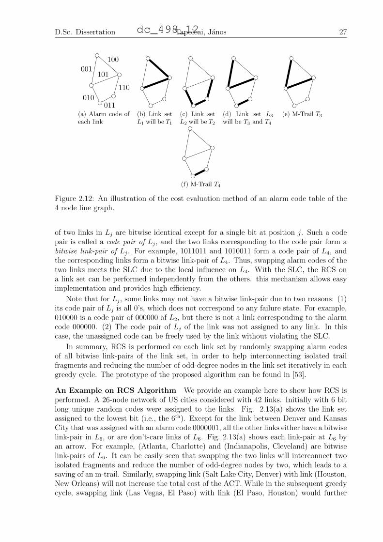
D.Sc. Dissertation Tapolcai, Janos 27
001
010
011
100
101
110
(a) Alarm code ofeach link
(b) Link setL1 will be T1
(c) Link setL2 will be T2
(d) Link set L3
will be T3 and T4
(e) M-Trail T3
(f) M-Trail T4
Figure 2.12: An illustration of the cost evaluation method of an alarm code table of the4 node line graph.
of two links in Lj are bitwise identical except for a single bit at position j. Such a codepair is called a code pair of Lj, and the two links corresponding to the code pair form abitwise link-pair of Lj. For example, 1011011 and 1010011 form a code pair of L4, andthe corresponding links form a bitwise link-pair of L4. Thus, swapping alarm codes of thetwo links meets the SLC due to the local influence on L4. With the SLC, the RCS ona link set can be performed independently from the others. this mechanism allows easyimplementation and provides high efficiency.
Note that for Lj, some links may not have a bitwise link-pair due to two reasons: (1)its code pair of Lj is all 0’s, which does not correspond to any failure state. For example,010000 is a code pair of 000000 of L2, but there is not a link corresponding to the alarmcode 000000. (2) The code pair of Lj of the link was not assigned to any link. In thiscase, the unassigned code can be freely used by the link without violating the SLC.
In summary, RCS is performed on each link set by randomly swapping alarm codesof all bitwise link-pairs of the link set, in order to help interconnecting isolated trailfragments and reducing the number of odd-degree nodes in the link set iteratively in eachgreedy cycle. The prototype of the proposed algorithm can be found in [53].
An Example on RCS Algorithm We provide an example here to show how RCS isperformed. A 26-node network of US cities considered with 42 links. Initially with 6 bitlong unique random codes were assigned to the links. Fig. 2.13(a) shows the link setassigned to the lowest bit (i.e., the 6th). Except for the link between Denver and KansasCity that was assigned with an alarm code 0000001, all the other links either have a bitwiselink-pair in L6, or are don’t-care links of L6. Fig. 2.13(a) shows each link-pair at L6 byan arrow. For example, (Atlanta, Charlotte) and (Indianapolis, Cleveland) are bitwiselink-pairs of L6. It can be easily seen that swapping the two links will interconnect twoisolated fragments and reduce the number of odd-degree nodes by two, which leads to asaving of an m-trail. Similarly, swapping link (Salt Lake City, Denver) with link (Houston,New Orleans) will not increase the total cost of the ACT. While in the subsequent greedycycle, swapping link (Las Vegas, El Paso) with link (El Paso, Houston) would further
dc_498_12

28 Tapolcai, Janos D.Sc. Dissertation
reduce the number of m-trails through the RCS and thus possibly reduce the total cost.With more greedy steps on those link pairs and don’t-care links of L6, it is possible to forma single m-trail corresponding to the 6th bit in the ACT while keeping all other link setsnot modified. By iterating the greedy process for each bit in the ACT, the algorithm canguarantee to obtain an m-trail solution for each bit in the ACT. The solution quality willdepend on the success rate threshold defined in Step (6) in Fig. 2.11. The effectivenessand efficiency of the proposed algorithm will be further demonstrated in the next section.
This link has nobitwise link-pairbecause its errorcode is 000001
(a)
Seattle
San Francisco
Chicago
New York
Los Angeles
Las Vegas
Salt Lake City
Denver Kansas City
Oklahoma City
Cleveland
St. Louis
WashingtonD.C.
Boston
Charlotte
Detroit
Toronto
Atlanta
Indianapolis
Houston
DallasEl Paso
Nashville
Miami
Minneapolis
New Orleans
(b)
Figure 2.13: Link set 6 (a) after random coding (b) after greedy random code swappingfor link set 6 in the ACT.
Performance Evaluation of RCA-RCS
Extensive simulation on thousands of different random topologies was conducted toverify the proposed algorithm. Specifically, we (1) demonstrated the solution quality ofthe proposed algorithm by comparing to the ILP in [27]; and (2) investigate impacts oftopology diversity on m-trail solutions.
Quality of Solution We investigated the quality of m-trail solutions generated by theproposed algorithm and its relation with the granted computation time. Also, comparisonwas made between the results by our algorithm and by the ILP in [27]. A server with3GHz Intel Xeon CPU 5160 was used on two typical networks: SmallNet (10 nodes, 22links) and ARPA2 (21 nodes, 25 links). Fig. 2.14 shows the quality of m-trail solutionsin terms of the total cost defined in Eq. 1 versus the granted running time by taking costratio γ = 5. Each little data interval in Fig. 2.14 is 95% confidence interval around themean of 30 experiments. The ILP solutions for the two networks under the same conditionwere also plotted for comparison.
With the RCS mechanism, the algorithm can achieve better results (i.e., smaller totalcost) when longer computation time was granted in both networks. The simulation resultsconfirmed our expectation. Interestingly, the proposed algorithm has generated evenbetter solutions than the ILP, while the running time is shorter by several orders. Thisexplicitly demonstrates the superiority of the proposed algorithm in terms of both solutionquality and required running time against the ILP. Note that the ILP results in theexample have nonzero gap-to-optimality of 4.17% in SmallNet and 20.41% in ARPA2,which cannot be erased only with dramatically increased running time. On the otherhand, the proposed algorithm spent about 0.01 seconds and 1 seconds to achieve the
dc_498_12

D.Sc. Dissertation Tapolcai, Janos 29
same total cost in the SmallNet and ARPA2, respectively, compared with 1,543 secondsand 9,573 seconds by the ILP.
T4T2
T5
T6
T1
T3
T6T4T1T2
T3
T5T7
T8
(a)
(b)
70
72
74
0.001 0.01 0.1 1 10 100 1000 10000
Tot
alC
ost
Running Time in [sec]
SmallNet
HeuristicILP [27]
(c)
90
100
110
0.01 0.1 1 10 100 1000 10000Running Time in [sec]
ARPA2
HeuristicILP [27]
(d)
Figure 2.14: The best heuristic solutions for SmallNet with cost of 69 and ARPA2 withcost of 87. In comparisons the ILP resulted 72 with 4.17% gap-to-optimality for andSmallNet and 98 with 20.41% for ARPA2.
Topology Diversity on M-Trail Solutions This section demonstrates the impact onm-trail solutions due to topology diversity. A huge number of experiments on thousandsof randomly generated topologies were conducted. Fig. 2.15 shows the minimal numberof m-trails versus network density on topologies with 50 nodes. The network connectivitywas increased starting from a backbone ring with 50 nodes and 50 links to a fully meshedtopology with 50 nodes and 1,225 links, where one or a few links were randomly addedto the topology for each data set. To make it statistically meaningful, every data intervalin Fig. 2.15 is 95% confidence interval around the mean of 20 different topologies eachobtained by randomly adding the same number of links to the backbone ring. We observedthat the normalized length of the alarm code (i.e., from the length of alarm code wesubtracted dlog2 (|E|+ 1)e) dramatically goes down when we add 50 to 100 links, orincrease the nodal degrees from 2 to 3. See Fig. 2.15(a) and Fig. 2.15(b), respectively.The length of the alarm code approaches the lower bound (i.e., dlog2 (|E|+ 1)e) when γis large enough. From Fig. 2.15(a) and (b), we have also observed that when γ is small,the confidence interval for each data is larger than in the case of larger γ. This indicatesthe fact that both monitoring cost and bandwidth cost are more sensitive to differentamounts of degree-2 nodes in the network, possibly due to the interplay between the twoobjectives in the cost function of Eq. (2.1).
Fig. 2.15(c) shows the normalized cover ratio (i.e., the sum of cover length of all m-trails divided by |E|) versus average nodal degree. We have seen that the cover ratio
dc_498_12

30 Tapolcai, Janos D.Sc. Dissertation
slightly increases when the average nodal degree is increased from 2 to 9 for all the threeγ values. Particularly, the cases with γ = 5 and 10 have better suppressed the increaseof cover length ratio, which demonstrates the effectiveness in the tradeoffs between thelength of the alarm code and bandwidth cost by manipulating the cost ratio γ.
0
5
10
15
20
25
50 70 90 110 130 150 170 190 210 230
#m
-tra
ils
-lo
g2|E|
Number of Edges
γ = 5γ = 10
γ = 1000
(a) Normalized length of alarm code versus number of links
0
2
4
6
8
10
12
14
16
2 3 4 5 6 7 8 9
#m
-tra
ils
-lo
g2|E|
Average Nodal Degree
γ = 5γ = 10
γ = 1000
(b) Normalized length of alarm code versus theaverage nodal degree
2.4
2.6
2.8
3
3.2
3.4
3.6
3.8
4
2 3 4 5 6 7 8 9
Norm
.C
over
Len
gth
Average Nodal Degree
(c) Normalized cover ratio versus average nodaldegree
Figure 2.15: Simulation on random topologies with 50 nodes.
Fig. 2.16 shows the m-trail solutions with different numbers of nodes in the networktopologies. Fig. 2.16(a) and (b) shows the length of the alarm code versus the number oflinks. Clearly, when γ = 1000, the length of the alarm code is only affected by the numberof links when it is small, while quickly converges to dlog2(|E|+ 1)e when the number ofadded links is increasing, regardless the number of nodes in the topology. Moreover, thelength of alarm code is always dlog2(|E|+ 1)e in case the network does not contain anynode with a nodal degree 2 or smaller, which also verifies the observations. On the otherhand, when γ is small, the convergence becomes slower, and the length of alarm codedeviates more from dlog2(|E|+ 1)e as γ is reduced.
Fig. 2.16(c) shows the results of the experiment, on the relationship between normal-ized length of the alarm code and total number of degree-2 nodes in the topologies with20, 30, 40, 50, and 60 nodes, altogether resulting 5,320 different random topologies. γwas set to 1,000. Each data point was obtained by averaging the results on 20 randomlygenerated topologies of the same total number of degree-2 nodes. We observed that all thetopologies with different numbers of nodes require more m-trails for UFL as the numberof degree-2 nodes grows, which meets our expectation. Interestingly, it is observed thatall the topologies have to take similar normalized length of alarm code for UFL given thesame number of degree-2 nodes. This indicates a serious impact on m-trail solutions due
dc_498_12

D.Sc. Dissertation Tapolcai, Janos 31
5
10
15
20
25
30
35
20 40 60 80 100 120 140 160 180 200 220 240
Nu
mb
erof
M-T
rails
Number of Edges
(a) γ = 1000
5
10
15
20
25
30
35
20 40 60 80 100 120 140 160 180 200 220 240
Nu
mb
erof
M-T
rails
Number of Edges
(b) γ = 5
-5
0
5
10
15
20
25
30
1 10 20 30 40 50 60
#m
-tra
ils
-lo
g2|E|
Total Stub Length
Total degree-2 nodes2
20 node networks30 node networks40 node networks50 node networks60 node networks
(c) Normalized length of alarm code versus total degree-2 nodes
Figure 2.16: The length of alarm code versus the number of added links for topologies of20, 30, 40, 50, and 60 nodes.
dc_498_12

32 Tapolcai, Janos D.Sc. Dissertation
to the number of degree-2 nodes in a topology. Based on these experiments the followingrelationship can be taken as a rule of thumb for approximating the normalized length ofthe alarm code in a random network topology when γ is very large:
b = #m-trail ≈ dlog2(|E|+ 1)e+#degree-2 nodes
2(2.8)
Note that the above rule of thumb does not hold for every graph because the con-struction in Section 2.2.2 is a counterexample.
2.3 Unambiguous Failure Localization for Multiple
Failures
2.3.1 Problem Definition
The alarm code of a multi-link SRLG is the bitwise OR, denoted by ∨, of the alarmcodes of all links in the SRLG. This corresponds to the fact that a monitor alarms if thecorresponding monitoring lightpath traverses through any link in the SRLG that is hitby the failure event. Thus, each SRLG z can be assigned with an alarm code as follows
Az =∨e∈Z
Ae ,
where∨
denotes the bitwise OR operator. The UFL constraint in this general caserequires every alarm code of each SRLG to be unique.
2.3.2 UFL for SRLG Failure with Bm-Trail
In general, an effective monitoring structure allocation method must satisfy the fol-lowing two requirements, either in a single step or one after the other:
(R1): Every SRLG should be uniquely coded.
(R2): Each monitoring structure must be an eligible fragment of network topology inwhich a lightpath can travel along from the transmitter to the receiver.
Note that in addition to (R1) and (R2), there could be some other constraints dueto specific user design premises, such as the length limitation due to the deployment ofoptical generators/retransmitters, the locations of monitoring nodes [35, 40], and use ofworking lightpaths (i.e., live connections) for failure state correlation [35, 42].
An integer linear program can be developed that satisfies both (R1) and (R2) in asingle step [22, 27, 38]. In particular, [27] is the first study that suggested to using freelyrouted open-loop un-directed supervisory lightpaths (called m-trail) for single-link SRLGfailure localization. All the three studies formulated the supervisory ligthpath allocationproblem into Integer linear programs (ILPs), which is unfortunately subject to intolerablylong computational time even in very small topologies. Thus people have turned to thedesign of heuristics in solving the problem. The previously reported solutions can bedivided into two categories according to their design principles. The first one manipulatesan accumulation mechanism such that (R2) is ensured at the beginning, while the goalof the heuristics is to satisfy (R1) [30, 35, 36]. In the second design category, (R1) isintrinsically ensured at the beginning while leaving (R2) as a goal [5].
dc_498_12

D.Sc. Dissertation Tapolcai, Janos 33
The bm-trail formation problem is a structured variant of the combinatorial grouptesting (CGT) process [54, 55]. In [30] the problem was taken as combinatorial grouptesting on graphs. The idea of group testing dates back to World War II when millionsof blood samples were analyzed to detect syphilis in US military. In order to reduce thenumber of tests it was suggested to pool the blood samples. From algorithmic aspectsthere are two significant differences between the tasks of pooling blood samples and mon-itoring of a group of links in a graph: (1) the blood samples can be pooled arbitrarily,while the monitored links must be connected and even in a valid shape, (2) the monitorsare always pre-configured, and the probing is performed simultaneously without knowingthe result of other tests (non adaptive CGT).
The primary goal of any CGT algorithm is to identify defective items among a givenset of items through as few tests as possible. In this case the set of items are the links ofa graph, the defective items are the failed links, and the tests are monitoring structures(e.g., bm-trails). The first general CGT method was given by Hwang and T. Sos [54],while the shortest real-world problem size non-adaptive CGT codes were developed byEpstein, Goodrich and Hirschberg [56].
In [30], with the help of non-adaptive combinatorial group testing (CGT) construc-tions, the authors conducted an indepth theoretical bound analysis on the problem, inwhich each link is assigned with multiple codes in a graph with at least d+1 disjoint span-ning trees. Therefore, the construction in [30] can only be applied to very densely meshedtopologies. For example, the network has to be as densely meshed as (2d+ 2)-connectedin order to accommodate d + 1 disjoint spanning trees, which results in (d + 1) · j bitsassigned to each link for achieving UFL of SRLGs with up to d links, where j is the CGTcode length. Obviously, such a method of assigning each link d + 1 CGT codes can fitwell into theoretical analysis, but it can hardly be applied in most practical scenarios.
The studies in [35, 36] set their goal in minimizing the number of monitoring locations(MLs). For example, to localize failure of SRLG with up to 2 links (i.e., d = 2), all the3- and 4-connected subgraphs should be identified, and almost each subgraph needs anML at an arbitrarily chosen node in the subgraph. With each ML determined, graphtransformation is performed such that the MLs are merged into a supernode (denotedas m), and cycles are cumulatively added into the transformed graph one by one viaSuurballe’s [57] algorithm. To distinguish two SRLGs w1 and w2, a cycle must be disjointfrom w2 while passing m and l, where l is a link randomly selected from w1 \ w2. In theworst case this leads to O(|SRLG|2) of cycles to distinguish all the SRLGs, where |SRLG|is the number of SRLGs considered in the network. Thus, the worst time complexity isO(|SRLG|2 · |V |2), where |V | is the number of nodes in network, and the term O(|V |2)corresponds to the complexity of Suurballe’s algorithm. The computation complexitybecomes O(|E|2d · |V |2) if every multiple failure with up to d links should be localized,where |E| is the number of links.
The approach taken in [5] (see also Section 2.2.7) is the first study following thesecond design principle, where the code uniqueness of each link (as defined in (R1)) is firstguaranteed, while an algorithm was given for the formation of each monitoring structurein the context of m-trail. A superb performance was witnessed in [5] by employing randomcode assignment (RCA) and random code swapping (RCS) for localizing any link failure.In specific, the RCA algorithm forms the j-th m-trail by randomly swapping a link codewith its bitwise code pair at the j-th position. For example, the codes ”11010110” and”11000110” form a bitwise code pair at the 4-th position. Note that such a RCS algorithm
dc_498_12

34 Tapolcai, Janos D.Sc. Dissertation
in [5] can only work when single-link failures are considered and it simply fails in presenceof the code dependency among overlapped SRLGs, which is the most critical task to beaddressed in this section.
This sections follows the second design category in order to take advantage of theextremely flexible structure of bm-trails in solving the problem.
2.3.3 The CGT-GCS Heuristic Approach for M-Trail Allocation
The proposed bm-trail allocation method follows the second design principle, whereCGT codes generated by [56, 54] are assigned to each link to ensure (R1). After the ran-dom code assignment, (R2) is pursued by way of greedy code swapping (GCS). Althoughseemingly similar to that in [5], the proposed approach is much different in both stagesof code generation and code swapping.
Fig. 2.17 is a flowchart that summarizes the proposed approach. In Step (1), the CGTcode construction GEN CGT generates a number of k d-separable codes of a length J bits,denoted as C. The input parameter |E| ensures that the code length J is the smallest
such that k ≥ |E|. Note that the property of d-separability ensures uniqueness of thebitwise OR of up to d codes in set C, which is required in (R1). In Step (2), an alarmcode table is formed by randomly selecting |E| out of k codes from C, which are furtherassigned to all the links. The group of |E| codes taken by the links is denoted as A, whilethe group of rest k − |E| unassigned codes is denoted as code set U , where U = C \ A.
With a CGT code of length J at each link, the best situation is that each bit position ofthe link can lead to an m-trail, and in this case there are totally J m-trails correspondingto the code assignment. But this is not likely to happen due to the random assignmentof the codes at the beginning. Our method solves the m-trail formation problem by GCSstarting in Step (3), which ensures (R2).
In Step (3), each link is categorized with one of the four attributes (i.e., isolated,leaf, bridge, and detour) in each bit position according to A. Next in Step (4), codepair (ae, Cx), where ae ∈ A and Cx ∈ C, is arbitrarily selected and checked in functionCostREval one by one to see how much cost reduction can be achieved by possibly swap-ping each code pair. The code pair with the steepest cost reduction after swapping is kept(i.e., ∆M). If ∆M is no less than γ and at least one bm-trail can be merged or removed,the two codes are swapped using function SWP, such that A is updated accordingly in Step(6) and the program then goes back to Step (3). Otherwise, the program returns the bestresult (i.e., A with the least bm-trails) and terminates.
Note that an eligible code swapping could be either a swapping between the codes bothin A (i.e., Cx ∈ A) or replacement of the link code with an unused one (i.e., Cx ∈ U).Steps (3), (4), (5), and (6) form a loop such that the largest cost reduction can be achievedin each iteration of code swapping.
Greedy Code Swapping (GCS)
To carry out m-trail formation, GCS is devised to greedily swap codes of two linkssuch that the coverage constraint at each bit position can be satisfied while the resultantsolution quality can be progressively improved according to the cost function Eq. (1).Such an iterative swapping process continues until a given condition is satisfied.
The cost reduction evaluation for each code swapping serves as an important buildingblock in the proposed GCS mechanism, which guides the m-trail formation process ateach link set. In swapping each code pair of two links, a set of regulations is necessary,
dc_498_12
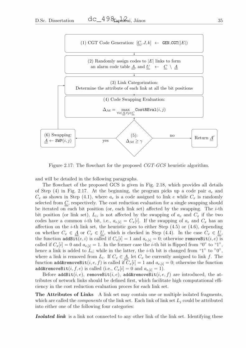
D.Sc. Dissertation Tapolcai, Janos 35
(1) CGT Code Generation: [C, J, k] ← GEN CGT(|E|)
(2) Randomly assign codes to |E| links to forman alarm code table A, and U ← C \ A
(3) Link Categorization:Determine the attribute of each link at all the bit positions
(4) Code Swapping Evaluation:
∆M = max∀i∈A,∀j∈C
CostREval(i, j)
(5):∆M ≥ γ
(6) Swapping:A ← SWP(i, j)
Return A′yes
no
Figure 2.17: The flowchart for the proposed CGT-GCS heuristic algorithm.
and will be detailed in the following paragraphs.The flowchart of the proposed GCS is given in Fig. 2.18, which provides all details
of Step (4) in Fig. 2.17. At the beginning, the program picks up a code pair ae andCx as shown in Step (4.1), where ae is a code assigned to link e while Cx is randomlyselected from C, respectively. The cost reduction evaluation for a single swapping shouldbe iterated on each bit position (or, each link set) affected by the swapping. The i-thbit position (or link set), Li, is not affected by the swapping of ae and Cx if the twocodes have a common i-th bit, i.e., ae,[i] = Cx[i]. If the swapping of ae and Cx has anaffection on the i-th link set, the heuristic goes to either Step (4.5) or (4.6), dependingon whether Cx ∈ A or Cx ∈ U , which is checked in Step (4.4). In the case Cx ∈ U ,the function addBit(e, i) is called if Cx[i] = 1 and ae,[i] = 0; otherwise removeBit(i, e) iscalled if Cx[i] = 0 and ae,[i] = 1. In the former case the i-th bit is flipped from “0” to “1”,hence a link is added to Li; while in the latter, the i-th bit is changed from “1” to ”0”,where a link is removed from Li. If Cx ∈ A, let Cx be currently assigned to link f . Thefunction add&removeBit(i, e, f) is called if Cx[i] = 1 and ae,[i] = 0; otherwise the functionadd&removeBit(i, f, e) is called (i.e., Cx[i] = 0 and ae,[i] = 1).
Before addBit(i, e), removeBit(i, e), add&removeBit(i, e, f) are introduced, the at-tributes of network links should be defined first, which facilitate high computational effi-ciency in the cost reduction evaluation proces for each link set.
The Attributes of Links A link set may contain one or multiple isolated fragments,which are called the components of the link set. Each link of link set Lj could be attributedinto either one of the following four categories:
Isolated link is a link not connected to any other link of the link set. Identifying these
dc_498_12
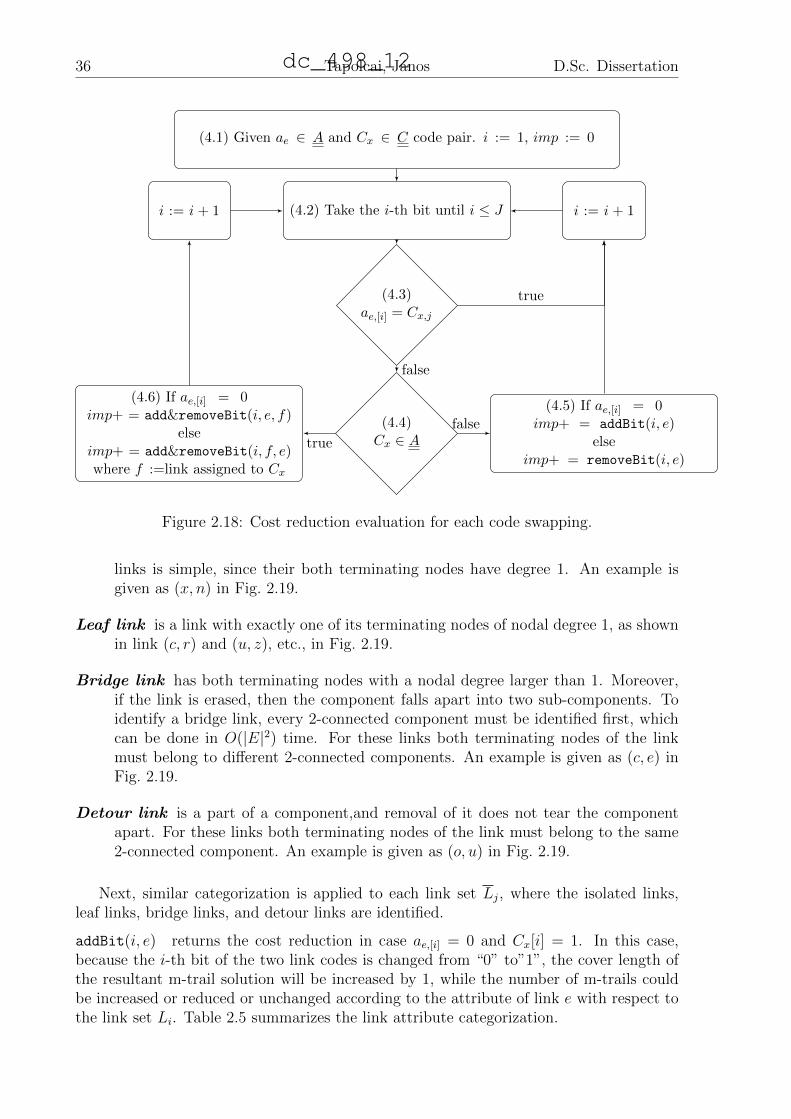
36 Tapolcai, Janos D.Sc. Dissertation
(4.1) Given ae ∈ A and Cx ∈ C code pair. i := 1, imp := 0
(4.2) Take the i-th bit until i ≤ J i := i + 1i := i + 1
(4.3)ae,[i] = Cx,j
(4.4)Cx ∈ A
(4.5) If ae,[i] = 0imp+ = addBit(i, e)
elseimp+ = removeBit(i, e)
(4.6) If ae,[i] = 0imp+ = add&removeBit(i, e, f)
elseimp+ = add&removeBit(i, f, e)where f :=link assigned to Cx
true
false
false
true
Figure 2.18: Cost reduction evaluation for each code swapping.
links is simple, since their both terminating nodes have degree 1. An example isgiven as (x, n) in Fig. 2.19.
Leaf link is a link with exactly one of its terminating nodes of nodal degree 1, as shownin link (c, r) and (u, z), etc., in Fig. 2.19.
Bridge link has both terminating nodes with a nodal degree larger than 1. Moreover,if the link is erased, then the component falls apart into two sub-components. Toidentify a bridge link, every 2-connected component must be identified first, whichcan be done in O(|E|2) time. For these links both terminating nodes of the linkmust belong to different 2-connected components. An example is given as (c, e) inFig. 2.19.
Detour link is a part of a component,and removal of it does not tear the componentapart. For these links both terminating nodes of the link must belong to the same2-connected component. An example is given as (o, u) in Fig. 2.19.
Next, similar categorization is applied to each link set Lj, where the isolated links,leaf links, bridge links, and detour links are identified.
addBit(i, e) returns the cost reduction in case ae,[i] = 0 and Cx[i] = 1. In this case,because the i-th bit of the two link codes is changed from “0” to”1”, the cover length ofthe resultant m-trail solution will be increased by 1, while the number of m-trails couldbe increased or reduced or unchanged according to the attribute of link e with respect tothe link set Li. Table 2.5 summarizes the link attribute categorization.
dc_498_12

D.Sc. Dissertation Tapolcai, Janos 37
0101
0110
1001
1010
1000
0100
0011
1111
0001
0010
1100
0111
1011
11011110
isolated leaf
leaf
leaf
leafbridge
bridge
bridge
detour
leaf
leaf
leaf
leaf
c
a
er
s
n
z
x
u
o
w
v
leaf leaf
Figure 2.19: An example on link attribute categorization for fast cost reduction evaluationon code swapping.
Table 2.5: Table lookup of addBit(i, e)Attribute of e for Li # of m-trails
isolated increased by 1leaf unchanged
bridge decreased by 1detour unchanged
removeBit(i, e) returns the cost reduction in case ae,[i] = 1 and Cx[i] = 0. Because thei-th bit is changed from “1” to “0”, the cover length is decreased by 1, while the numberof bm-trails should be updated according to the attribute of e with respect to Li. This issummarized in Table 2.6.
Table 2.6: Table Lookup of removeBit(i, e)Attribute of e for Li # of bm-trails
isolated decreased by 1leaf unchanged
bridge increased by 1detour unchanged
add&removeBit(i, e, f) is for the cost reduction evaluation in the event that link e isadded and another link f is removed from Li. After the swapping the cover length isunchanged while the number of m-trails changes according to the attributes of both links.This is provided in Table 2.7.
In summary, the proposed GCS swaps a code pair with the steepest cost reductionlarger than a threshold γ based on the proposed link attribute categorization and tablelookup process, which greedily approaches to better performance according to Eq. (2.1).With GCS, very high computational efficiency can be achieved thanks to the constant timecomplexity in evaluating each code pair, which will be detailed in the next subsection.The prototype of the proposed algorithm can be found in [53].
dc_498_12

38 Tapolcai, Janos D.Sc. Dissertation
Table 2.7: Table lookup of add&removeBit(i, e, f)add e remove fAttrib. Attrib. # of bm-trailsof Li of Li
isolated
isolated unchangedleaf increased by 1bridge increased by 2detour increased by 1
leaf
isolated decreased by 1 if e and f are not adjacent links, oth-erwise unchanged
leaf Either unchanged or increased by 1, if e is con-nected to f . See link (r, n) and (r, c) on Fig. 2.19 as anexample.
bridge increased by 1detour unchanged
bridge
isolated decreased by 2 if e and f are disjoint, otherwise in-creased by 1
leaf Either decreased by 1, or unchanged if e is adjacent tof . See link (o, w) and (o, s) on Fig. 2.19 as an example.
bridge unchangeddetour decreased by 1
Detour
isolated decreased by 1leaf unchangedbridge Either decreased by 1 or unchanged if e reconnects
the detached sub-components.See links (o, u) and (u,w) in Fig. 2.19 as an example.Lemma 5 provides a method to determine a bridge.
detour unchanged
Computational Complexity Analysis
The cost reduction evaluation is performed in each code swapping, which dominatesthe computational complexity of the heuristic algorithm. Next we prove three claimsneeded for a lemma that describes the computational complexity of the cost reductionevaluation process for a single code swapping.
Lemma 5. The complexity of CostREval(i, j) is O(1).
Proof. In the table lookup process for each code swapping, it can be intuitively verifiedthat every entity in the table can be performed in constant time.
Note that it is not obvious that the execution of add&removeBit(i, e, f) with e andf as a detour and bridge link, respectively, only takes constant time complexity. It isachieved via a pre-calculation process performed beside the link attribute categorizationin Step (2).
For link set Lj, we need to determine the relationship between any node and a bridgelink of aj = 1, which can be done in constant time. For example in Fig. 2.19(a), (c, e)is a bridge link of Lj, and removal of it separates Lj into two isolated components thatform two m-walks with nodes a, c, r and e, s, respectively. Such a function can be
dc_498_12

D.Sc. Dissertation Tapolcai, Janos 39
implemented by storing the reach and leave order of each node in the DFS algorithm.As shown in Fig. 2.20 as an example, the reach order of the DFS is written on the topof nodes, while the leave order is below the nodes. Let IR and IR denote the largestreach and the smallest leave order indices of the bridge. Every node with a reach andleave index at least IR and at most IL belongs to one side of bridge. As exemplified inFig. 2.20, we have IR = 2 and IL = 8, thus a, r, c are in one sub-component.
bridgec
a
er
s2 1
3
4
67
8 1211
10
Figure 2.20: Leave and reach order of the DFS algorithm. The links of Lj are drawn withthick lines.
Lemma 6. The complexity of Step (2) is O(|E| log |E|).
Proof. Clearly, a DFS function for detecting the components in each link set is in O(|E|)time complexity. Since each bridge link connects to two 2-connected components, toidentify a bridge link, we must identify the corresponding two 2-connected componentsfirst, which can be done in O(|E|) time complexity[58]. Also, such a check needs to gothrough each bit position, which multiplies the complexity by a factor of log |E|. Thus,the lemma is proved.
Lemma 7. The complexity of Step (3) is O(|E|2 log |E|).
Proof. For each code and link pair, the proposed method can evaluate the possible costreduction with a constant time (O(1)) according to Lemma 5. Since the overall timecomplexity is O(|E| · #codes · J), and since #codes = O(|E|), we have the worst casecomplexity of Step (3) as O(|E|2 log |E|).
Lemma 8. The computational complexity of a cost reduction evaluation process for asingle swapping is O(|E|2 log |E|).
Proof. It is a direct consequence of the above three lemmas.
It is clear that the number of isolated components (or m-trails) in the initial randomcode assignment for each bit position cannot be more than |V |/2. This is because eachisolated component consists of at least a single edge and two nodes, where |V | is thenumber of nodes in the network. After each loop (defined in Steps (3), (4), (5), and (6) ofFig. 3), at least one m-trail is determined and erased from the link set; thus, the maximum
number of code swappings should be upper bounded by |V |2·J , where J is the code length
(in bits). Note that J is in the order of O(d · log |E|) according to the CGT construction.By considering the complexity of each code swapping as O(|E|2 log |E|), the overall worstcase complexity in the proposed method is O(|V ||E|2 · d · log2 |E|). Compared with thescheme in [35, 36] with a complexity of O(|E|2d · |V |2), the proposed approach can achievemuch better efficiency.
dc_498_12

40 Tapolcai, Janos D.Sc. Dissertation
Performance Evaluation of CGT-GCS
Simulations on hundreds of randomly generated planar 2-connected network topolo-gies were conducted. The network topologies were generated with lgf gen, a randomgraph generator of LEMON [59], which randomly generates realistic planar 2-connectednetworks. The networks are classified according to the girth of the graph, denoted by g,which is the length of a shortest cycle contained in the graph. Clearly, a smaller value of gyields a more densely meshed topology. Fig. 2.21(a) shows the statistics of the randomlygenerated topologies. See also Fig. 3.5 for example network topologies with different girth.It is found that the average nodal degree is 3.0 for dense networks (g = 7) and 4.0 forsparse networks (g = 4).
In the simulation, the proposed scheme is denoted as CGT-GCS 1, CGT-GCS 2 andCGT-GCS 3 for failure localization of SRLGs with up to 1, 2, and 3 links, respectively,where the CGT codes based on d-separable constructions with d = 1, d = 2, and d = 3are employed. CA1 and CA2 corresponds to the method that each bi-directional m-trailis allocated one after the other to distinguish each pair of SRLGs using any Dijkstra’salgorithm based scheme, such that UFL for single-link SRLGs and for both single- anddouble-link SRLGs can be achieved, respectively. The method is generic and has beenconsidered in a number of previously reported studies [35, 60, 26]. We have also imple-mented the construction in [30] that used disjoint spanning trees, denoted as DSTC. Theconstruction provides an upper bound for (d+ 1)-connected topologies, but is invalid fortopologies with any node of a smaller nodal degree than (d + 1). The upper bound isgiven by (d+ 1) . . . J , where J is the length of the CGT codes employed.
Fig. 2.21(b) shows the lengths of CGT codes (i.e., J) versus the number of links |E|of the corresponding topology by the CGT code generator GEN CGT in [56], where thescenarios with d = 2 are presented. It is intuitive that when SRLGs with more links areconsidered, longer CGT codes are required for each link.
0
50
100
150
200
250
300
20 50 100
#li
nks
#nodes
g=3g=7
(a) Statistics of the random topologies. The densenetworks have girth g = 3, while for the sparsenetworks g = 7.
020406080
100120140160
20 200 300
#b
its
#links
CGT 3
CGT 2
(b) The length of CGT code (in bits) versus thenumber of links as an input to the CGT code gen-erator GEN CGT in [56]
Figure 2.21: Statistics on the input data.
The performance metrics employed in the comparison of the six schemes are the mini-mum number of m-trails required for achieve UFL and the running time. Both metrics areexamined with respect to different network sizes (i.e., the number of nodes) and topologydensities (i.e., g values), which will be presented in the following two subsections. Thesimulation has been done on over 800 randomly generated topologies, and each data wasobtained by averaging the results from 10 different topologies with a specific g value and
dc_498_12

D.Sc. Dissertation Tapolcai, Janos 41
number of nodes. A bar for each data in the charts is available for showing the range ofdata we obtained.
Number of M-Trails versus Network Size The performance in terms of the mini-mum number of m-trails is first investigated, and the results are shown in Fig. 2.22. First,we find that the number of m-trails increases when the network size grows, which is ob-served in all the cases. It clearly shows that the proposed approach achieve much betterscalability, where CGT-GCS 1, CA1, and CA2 have achieved far worse performance thanthat by CGT-GCS 1 and CGT-GCS 2, respectively, in both types of network topologies.
The superior performance of the proposed approach in minimizing the number of m-trails can be explained in two folds. First, the m-trails have the most flexible routingstructure that can fully explore the solution space. This serves as a critical factor inovercome the vicious effect of topology diversity. It can be attested that our scheme hasless advantage against the other two counterparts when network is sparsely connected (i.e.,g = 7), because there are less alternatives in allocating the m-trails. Second, because CA1
and CA2 have each monitoring lightpath sequentially allocated into the network using anshortest path routing algorithm, it lacks intelligence in exploring the design space andnetwork topology diversity. Third, DSTC [30] tries to ensure the code uniqueness of eachSRLG by useing d + 1 disjoint spanning trees, which is strongly limited by the topologyconnectivity. It is clearly shown that the construction can only yield valid solution in verydensely meshed topologies, while failed in most of the sparse topologies considered in thesimulation.
Running Time Fig. 2.23 shows the running time for obtaining the data in Fig. 2.22.It is observed that the proposed approach achieves much better computational efficiency,although CA2 can achieve performance closer to CGT-GCS 2 for sparser network topolo-gies. Also, CGT-GCS 3 takes much longer time than CGT-GCS 2 and any other case dueto a much longer CGT code with d = 3, as shown in Fig. 2.21(b). Recall that the costreduction evaluation in each code swapping has to go through all the link sets that are af-fected by the code swapping. Thus, the longer CGT code of each link yields an immediateincrease of running time in obtaining an m-trail solution.
Note that we tried to implement CA3 but failed due to the extremely long computa-tional time required for each data in the selected topologies. This clearly demonstrates su-perior scalability of the proposed approach which can achieve better capability in handlinga huge amount of SRLGs in densely meshed networks compared with its counterparts.
dc_498_12

42 Tapolcai, Janos D.Sc. Dissertation
0102030405060708090
20 50 100
#b
m-t
rail
s
#nodes
CA1
CGT-GCS 1
DSTC1
(a) g = 3 single failure
01020304050607080
20 50 100
#b
m-t
rail
s
#nodes
(b) g = 7 single failure
0
50
100
150
200
250
20 50 100
#b
m-t
rail
s
#nodes
CA2
CGT-GCS 2
DSTC2
(c) g = 3 double failure
20406080
100120140160
20 50 100
#b
m-t
rail
s
#nodes
(d) g = 7 double failure
0
100
200
300
400
500
600
20 50 100
#b
m-t
rail
s
#nodes
CGT-GCS 3
DSTC3
(e) g = 3 triple failure
50100150200250300350400
20 50 100
#b
m-t
rail
s
#nodes
(f) g = 7 triple failure
Figure 2.22: The number of bm-trails versus the number of nodes.
0.01
0.1
1
10
100
1000
10000
20 50 100
run
nin
gti
me
[sec
]
#nodes
CGT-GCS 3
CGT-GCS 2
CGT-GCS 1
CA2
CA1
(a) Dense networks
0.001
0.01
0.1
1
10
100
1000
10000
20 50 100
run
nin
gti
me
[sec
]
#nodes
(b) Sparse networks
Figure 2.23: The running time versus the number of nodes.
dc_498_12

Chapter 3
Distributed Single FailureLocalization in All-Optical MeshNetworks
3.1 Introduction
Unambiguous Failure Localization (UFL) is defined in all-optical mesh WDM networkswhere any link failure can be precisely and instantly identified via monitoring a set ofsupervisory lightpaths. Such capability in the network optical layer is highly desired inorder to meet the stringent requirement on service continuity and to support variousfailure-dependent restoration mechanisms [61, 62, 63].
Several UFL schemes have been proposed in Chapter 2. Using m-trails with bi-directional lightpaths in all-optical WDM networks has been proposed [30, 6, 64, 65];and all these studies set the destination node of each m-trail as the only node that candetect the status of the m-trail. This results in a fact that alarm dissemination is neededupon a failure event mostly via flooding and dedicated failure notification based on net-work layer signaling, such that the alarm code can be formed at a remote site or anynetwork node in order to localize the failure. Obviously, using electronic signaling inalarm bit collection incurs additional control complexity, operational overhead, and lowerrobustness of the system. The dependency on the upper layer signaling mechanism im-plies that these approaches leave the optical domain, which may cause problems. Such anissue was considered in [35], which aimed to minimize the number of monitoring locations(MLs) in order to reduce the alarm dissemination. Nonetheless, the research in [35] canhardly be applicable to the scenario where all the nodes are required to perform UFL inthe optical domain, and may yield solutions with multiple MLs in sparse networks, andin this case the MLs have to exchange their alarm bits via control plane signaling. Mostimportantly, the approach in [35] pays no attention to the number of required supervisorylightpaths which affects seriously the number of transmitters and the total cover length.
Motivated by the fact that UFL should be carried out completely in the optical do-main and be free from any control plane signaling effort, this section investigates anadvantageous scenario of all-optical failure localization using bi-directional m-trails. Herewe define Local UFL (L-UFL) at a node if the node can individually perform UFL basedon locally available on-off status of the traversing m-trails; and Network-Wide Local UFL(NL-UFL) in the network if every node is L-UFL capable. By assuming that any node
43
dc_498_12

44 Tapolcai, Janos D.Sc. Dissertation
T1 T2 T3
0 1
23
(a) Topology and m-trails
SRLG T1 T2 T3
(0, 1) 0 0 1(1, 2) 0 0 1(2, 3) 0 1 1(3, 0) 1 1 0
(b) Alarm code table (ACT) at node 0
Figure 3.1: Local-unambiguous failure localization (L-UFL) based on m-trails. Node 0 isthe monitoring location. The cover length is ‖T ‖ = 6.
along an m-trail can obtain the on-off status of the m-trail via optical signal tapping, allthe nodes traversed by the m-trail can share the on-off status of the m-trail. The proposedNL-UFL m-trail allocation problem is to find a set of m-trails such that every node canperform L-UFL based on the traversing m-trails.
The section first introduces the NL-UFL framework along with its possible applicationscenarios, and defines the NL-UFL m-trail allocation problem. To gain an understandingof the problem, we conduct bound analysis by proving optimal solutions in terms ofminimal cover length in a number of special graphs, such as lines, stars, and completegraphs, as well as the derivation of lower bounds in general graphs. Inspired by the optimalsolution for complete graphs, we develop a novel heuristic algorithm for solving the NWL-UFL m-trail allocation problem based on random spanning tree assignment (RSTA) andgreedy link swapping (GLS). Extensive simulation on thousands of randomly generatedtopologies is conducted to verify the proposed heuristic approach and examine the derivedlower bounds. The impact of network diversity is also investigated.
3.2 Problem Definition
3.2.1 Local Unambiguous Failure Localization (L-UFL)
L-UFL is an advanced application of m-trail deployment, where the UFL constraint isstricter while the shape constraint is the same as for UFL described in Section 2.1.2. Anode is said to be L-UFL capable if and only if the node can perform UFL by inspectingthe on-off status of the m-trails locally available. An m-trail is said to be locally availableat node n if it terminates in n. In the L-UFL problem the goal is to find a node withL-UFL. This node is called monitoring location (ML).
In many cases none of the nodes can serve as an ML, and thus the goal is to find asmallest set of nodes that altogether have sufficient information for UFL. As a consequenceof Theorem 8, any node can be the single ML in a 2-connected network to achieve L-UFLwith bm-trails for single link failures. The bandwidth cost is also considered in the L-UFLproblem, with significantly smaller weight compared to the number of MLs.
3.2.2 An L-UFL Example
Fig. 3.1 shows an example of L-UFL m-trail solution on the network of 2.1(a) forlocalizing any single link failure. Node 0 is chosen for monitoring location, and the localACT at node 0 is shown in Fig. 3.1(b). Here, every m-trail should terminate in node 0.
dc_498_12

D.Sc. Dissertation Tapolcai, Janos 45
3.2.3 State of the Art on L-UFL
The study in [35] set its goal to minimize the number of MLs, which is determinedby analyzing the connectivity among the 2- and 3-edge-connected components in thetopology. With each ML determined, a graph transformation is performed such that theMLs are merged into a supernode (denoted by m), and cycles are cumulatively added intothe transformed graph one by one via Suurballe’s algorithm. The method was extendedfor sparse SRLG in [36].
3.2.4 Network-Wide L-UFL
In Network-wide L-UFL (NL-UFL) every node has to be L-UFL capable. To achievethis the L-UFL condition is slightly relaxed by assuming that any node along a monitoringlightpath can obtain the on-off status of the lightpath via optical signal tapping. Thus, allthe nodes traversed by the lightpath can share the on-off status of the m-trail. It meansa node can locally inspect the on-off status of every traversing monitoring lightpath.
The task is to allocate monitoring lightpaths with minimum total cover length, suchthat the shape constraint is fulfilled (see also Section 2.1.2), and the NL-UFL constraintrequires unique alarm code for each SRLG at each node. The alarm code at node v ∈ Vfor SRLG z ∈ Z is denoted by avz, where avz = [avz,[1], a
vz,[2], . . . , a
vz,[bv ]] is a binary vector, bv
is the total number of m-trails traversing node v, and the jth bit of avz, denoted by avz,[j],is 0 if the j-th m-trail traversing node v is operating after failure z, and 1 otherwise.
Thus for each node v we define an ACT, denoted as Av, which is a |Z|× bv size matrixwith each row as avz, ∀z ∈ Z. Obviously b ≥ bv for each v ∈ V , as it is a sub-matrix of theglobal ACT. When any failure occurs and interrupts one or a number of m-trails, node vwill obtain a nonzero alarm code which uniquely identifies the failed SRLG.
The target function of the NL-UFL problem is the total cover length, denoted by‖T ‖. It is because NL-UFL does not rely on any upper layer signaling effort for alarmcode dissemination and, thus the length of alarm code is not as critical as that in UFLframework.
The following theorem indicates the feasibility of the approach in any 2-connectedgraph. The theorem demonstrates that an m-trail solution for single-link NL-UFL canalways be obtained in a connected graph.
Theorem 8. Given a connected graph, an m-trail solution for NL-UFL can always befound.
Proof. The necessity of the connectivity of the graph is trivial. For the sufficiency part, weneed to show that every node vs can achieve L-UFL. Formally, we have to prove that thefailure of an arbitrary link (vi, vj) can be unambiguously detected at vs using a suitablecollection of m-trails.
Indeed, after possibly renumbering the vertices we may assume, that vi is not fartherform vs than vj. Then let T1 be a (possibly empty) shortest path from s to vi. Note thatT1 does not contain the link (vi, vj). Also, let T2 = T1 ∪ (vi, vj). Then we have that(vi, vj) is faulty iff T2 gives an alarm signal and T1 does not. These events are obviouslyvisible at any vs and can be repeated for every link (vi, vj).
3.2.5 An NL-UFL Example
Fig. 3.2(a) shows an example of NL-UFL for any single-link SRLG using four m-trailsin a topology with 4 nodes. Fig. 3.2(b) shows the routes of the four m-trails T1, T2, T3, and
dc_498_12

46 Tapolcai, Janos D.Sc. Dissertation
T1 T2
T3T4
0 1
23
(a) M-trails
Link T1 T2 T3 T4
(0, 1) 1 1 0 0(1, 2) 0 1 1 0(2, 3) 0 0 1 1(3, 0) 1 0 0 1
(b) Route table
Link T1 T2 T3
(0, 1) 1 1 0(1, 2) 0 1 1(2, 3) 0 0 1(3, 0) 1 0 0
(c) ACT at node 1
Figure 3.2: Network-wide Local UFL (NL-UFL) via m-trails. The cover length is ‖T ‖ = 8.
T4. In our case, each of the four nodes can achieve single-link L-UFL by inspecting thelocally available on-off status of the traversing m-trails. For example, node 1 maintainsan ACT as shown in Fig. 3.2(c), where the on-off status of T1, T2, and T3 form an alarmcode of three bits which uniquely maps to each possible link failure event. If node 1 findsthat T1 and T2 become suddenly off while T3 is still on, link (0, 1) is considered down andcan be localized as defined in the first row of the ACT; if T1 and T2 are on while T3 is off(as shown in the third row of the ACT), link (2, 3) is considered down. Similarly, node 0,2, and 3 can perform UFL by maintaining their ACTs, each of which keeps the mappingbetween all the considered failure states and the on-off status of the traversing m-trails.
3.3 Bounds On Bandwidth CostThis section presents our bound analysis for cover length in the proposed NL-UFL m-
trail problem. We will first look into a lower bound on general connected graphs, followedby the optimal solutions for a number of special graph topologies: line, star and completegraphs.
3.3.1 Lower Bound for General Graphs
Theorem 9. Let T = T1, . . . , Tb be a valid m-trail solution for NL-UFL. We have
‖T ‖ ≥|V |∑j=1
|V |∑µ=1
µ− 1
µ(dlog2 δj(µ− 1)e − dlog2 δj(µ)e) (3.1)
where δj(µ) denotes the number of links whose shortest distance from node vj is µ.
Proof. Let the reputation of Ti be denoted by r(Ti), which represents the number of nodesalong m-trail Ti that are aware of the on-off status of Ti. A trivial upper bound on r(Ti)is |Ti|+ 1 if Ti is loopless; or formally
r(Ti) ≤ |Ti|+ 1. (3.2)
Let us define a matrix Ω with b columns and n rows, where
ωi,j =
|Ti|r(Ti)
the i-th m-trail traverses node vj,
0 otherwise.(3.3)
The length of Ti can be expressed as
|V |∑j=1
ωi,j =
|V |∑j=1
|Ti|r(Ti)
= |Ti|. (3.4)
dc_498_12

D.Sc. Dissertation Tapolcai, Janos 47
Thus we haveb∑i=1
|V |∑j=1
ωi,j =b∑i=1
|Ti| = ‖T ‖ (3.5)
As a lower bound on ωi,j according to Eq. 3.2, we have
ωi,j =|Ti|r(Ti)
≥ |Ti||Ti|+ 1
≥ 1
2(3.6)
Let us denote the set of m-trails passing through node vj by T j. Next, we give a lower
bound on∑b
i=1 ωi,j for each node vj, which is denoted by ωj, formally
ωj =b∑i=1
ωi,j =∑Ti∈T j
|Ti|r(Ti)
≥∑Ti∈T j
|Ti||Ti|+ 1
(3.7)
where Ti ∈ T j means that m-trail Ti passes through node vj. Note that the cover lengthis the sum of ωj for all nodes, formally
‖T ‖ =
|V |∑j=1
ωj, (3.8)
Let us denote the distance between node vj and link e ∈ E by δ(vj, e), which equalsto the length of the shortest path between node vj and the closest adjacent node of eplus 1. Without loss of generality, the distance can be simply measured in hops. Letδj(k) denote the number of links whose distance from node vj is at least k. For example,δj(1) = |E| as every link is at least 0 hop from the node, and δj(2) = |E| − ∆j, where∆j is the nodal degree of j. Let nj denote the maximum δ distance from node vj, thusδj(nj + 1) = 0 and δj(nj) > 0. Note that such nj always exist because there are nolinks with distance n − 1. Note that δj(µ) is a monotonically non-increasing function ofµ (i.e. δj(1) ≥ . . . ≥ δj(nj) ≥ 1). To localize any single failure at node vj among linkswhose distance from vj is at least µ− 1, there must be dlog2 δj(µ)e m-trails with at leasta distance of µ.
From T j we select dlog2 δj(nj)e m-trails whose length is at least nj. By Eq. (3.7) theycontribute to ωj at least
nj − 1
njdlog2 δj(nj − 1)e =
nj − 1
nj(dlog2 δj(nj − 1)e − dlog2 δj(nj)e).
In a similar manner, from the remaining m-trails in T j we may select as many asdlog2 δj(nj − 2)e − dlog2 δj(nj − 1)e m-trails whose lengths are at least nj − 2. Theircontribution to ωj is at least
nj − 2
nj − 1(dlog2 δj(nj − 2)e − dlog2 δj(nj − 1)e),
by Eq. (3.7) again. Continuing in this way for µ = nj, . . . , 1 we obtain a collection ofm-trails in T j such that the following inequality follows
ωj ≥nj∑µ=1
µ− 1
µ(dlog2 δj(µ− 1)e − dlog2 δj(µ)e) (3.9)
dc_498_12

48 Tapolcai, Janos D.Sc. Dissertation
By summing up ωj for every node according to Eq. (3.8) we get a lower bound on coverlength in Eq. (3.1).
Theorem 9 can be well applied when the average nodal degree is small (e.g., lessthan 6). We show in Section 3.4.3 that Theorem 9 can provide a lower bound in a form‖T ‖ ? ξ|V | log2 (|E|+ 1) where ξ is somewhere in [0.85, 0.95] for random networks withaverage nodal degree less than 6.
To further improve the above theorem, next we introduce a related CombinatorialGroup Testing (CGT) problem. We will first consider the lower bound on this generalizedversion of Combinatorial Group Testing (CGT) and then apply them to the NL-UFLrequirement at each node, which will give us a lower bound on the coverlength for generalgraphs. The key idea is to define a special cost function for the m-trails at each node suchthat the lower bound to meet the NL-UFL problem of each node can be summed up toget a lower bound on the total coverlength.
3.3.2 General Lower Bound for CGT
Let us consider a non-adaptive CGT problem where the goal is to find one faulty itemamong a set of items with group tests, where each group test is on a set of items andhas two an outcomes: the test contains a faulty item or not. Note that the NL-UFLproblem at each node n is a special version of CGT, where the tests are the m-trailspassing through n, and the items are the links. We have two additional constraints:
• The links must form a path in the topology, and
• Each of the links must have a non-zero code.
It is clear that a valid NL-UFL solution at node n is a valid CGT solution over links E.Next, let us formalize the CGT problem with a cost function on each test. The cost
of test Ti depends on its size according to a given cost function ω(). The input of theCGT problem is a set of items denoted by E = e1, . . . , em and a cost function ω, wherem = |E| is the number of items. The goal is to establish a set of b group tests, denotedby T1, . . . , Tb, where each group test consists of a set of items, such that a single faultyitem can be unambiguously identified according to the outcomes of the group tests. It isalso called separating test collection. Each test has a cost defined as follows
Definition 1. The cost of test Ti with ti = |Ti| is ω(ti), where function ω has the followingproperties:
(i) ω(1) = 1, meaning that test with one element has a unit cost.
(ii) ω(x + 1) ≥ ω(x) for every positive integer 1 ≤ x ≤ m − 1. Testing a larger groupcannot decrease the cost.
(iii) ω(x)x≥ ω(x+1)
x+1whenever 1 ≤ x < m.
The goal is to identify the faulty item with minimum cost:
Minimize Ω =b∑i=1
ω(ti) (3.10)
Note that much of the prior art focused on the cases with ω(t) = 1, i.e. the cost of atest does not depend on the number of items, and thus the goal is to reduce the numberof tests.
dc_498_12

D.Sc. Dissertation Tapolcai, Janos 49
Theorem 10. Suppose there are m > 1 items and assume (i)-(iii) holds for the costfunction ω. Then for the cost of finding precisely one faulty item with group tests is atleast
Ω ≥ min1≤x≤m
2
ω(x)(
log2 x+m
x− 1)
(3.11)
Proof. Let us sort the tests by descending size, so that T1 has the largest number of itemswhile Tb has the least: we assume that
t1 ≥ t2 ≥ · · · ≥ tb
where ti = |Ti| denotes the number of items in test Ti.Also, we may assume that ti ≤ m
2for every i. Indeed, a test set Ti with |Ti| ≥ m
2can
be replaced by its complementary set E \ Ti. The resulting test collection still remainsseparating if the original one was separating.
We build up the b × m matrix by adding the rows one-by-one, and in each step wecount the number of different columns in the matrix. Let fi denote the number of differentcolumns when the matrix has i rows, i.e. tests T1, . . . , Ti are present, the others are not.For convenience we set f0 = 1. Adding a row the number of different columns cannotdecrease, thus fi−1 ≤ fi for i = 1, . . . , b. As we have a separating system, all the mcolumns will be different when the last row is added, giving that fb = m.
When we add Ti, the number of different columns is at most doubled, hence fi ≤ 2fi−1,or
log2(fi)− log2(fi−1) ≤ 1 (3.12)
for i = 1, . . . , b.Similarly, by adding test Ti to the collection T1, . . . , Ti−1 can increase the number of
different columns in the matrix by at most ti, giving fi ≤ fi−1 + ti, or
fi − fi−1
ti≤ 1 (3.13)
for i = 1, . . . , b.Now fix an integer k with 1 ≤ k < b. We have
Ω =b∑i=1
ω(ti) ≥k∑i=1
ω(ti) (log2(fi)− log2(fi−1)) +b∑
i=k+1
ω(ti)
(fi − fi−1
ti
). (3.14)
We used (3.12) in the first sum, and (3.13) in the second.The sequence ω(ti) is nonincreasing for i = 1, . . . , b by (i) and our numbering of the
tests, hence
k∑i=1
ω(ti)(log2(fi)− log2(fi−1)) ≥k∑i=1
ω(tk)(log2(fi)− log2(fi−1)) = ω(tk) log2(fk). (3.15)
Similarly, the sequence ω(ti)ti
is nondecreasing because of (iii) and our numbering of thetests, giving that
b∑i=k+1
ω(ti)
(fi − fi−1
ti
)≥
b∑i=k+1
ω(tk+1)
(fi − fi−1
tk+1
)=ω(tk+1)
tk+1
(m− fk). (3.16)
dc_498_12

50 Tapolcai, Janos D.Sc. Dissertation
By substituting (3.15) and (3.16) into (3.14), we have
Ω ≥ ω(tk) log2(fk) +ω(tk+1)
tk+1
(m− fk) ≥ ω(tk)
(log2(fk) +
m− fktk
). (3.17)
This inequality is valid for any k with 1 ≤ k < b. Let we set now k to be the first indexj for which tj ≤ fj. Such index clearly exists and k < b because fb−1 ≥ m
2, while ti ≤ m
2
for every i. We need to consider two cases:(1) If fk−1 ≤ tk, then we have
Ω ≥ ω(tk)
(log2(fk) +
m− fktk
).
Note that tk ≤ fk ≤ 2fk−1 ≤ 2tk, hence for δ defined by fk = tk+δ we have 0 ≤ δ ≤ tk.Moreover,
Ω ≥ ω(tk)
(log2(tk + δ) +
m− tk − δtk
)= ω(tk)
(log2(tk + δ)− δ
tk+m
tk− 1
). (3.18)
On the interval 0 ≤ x ≤ 1 we have the inequality x ≤ log2(1 + x). We apply this forx = δ
tk. Note that 0 ≤ δ ≤ tk implies that 0 ≤ x ≤ 1. We obtain the following inequality
log2(tk + δ)− δ
tk≥ log2(tk + δ)− log2
(1 +
δ
tk
)=
= log2
(tk + δ
1 + δtk
)= log2
(tk + δtk+δtk
)= log2(tk). (3.19)
Substituting (3.19) into (3.18) we get
Ω ≥ ω(tk)
(log2(tk) +
m
tk− 1
).
(2) If tk < fk−1, then k > 1 because f0 = 1 by definition. Thus fk−1 < tk−1 and based on(3.17) we have
Ω ≥ ω(tk−1) log2(fk−1) +ω(tk)
tk(m− fk−1).
Since ω(t)t
is a nonincreasing function of t, we have
Ω ≥ ω(fk−1) log2(fk−1) +ω(fk−1)
fk−1
(m−fk−1) ≥ ω(fk−1)
(log2(fk−1) +
m
fk−1
− 1
). (3.20)
In both cases there is an integer x in the interval [1, m2
] such that
Ω ≥ ω(x)(
log2(x) +m
x− 1).
This is because fk−1 < tk−1 ≤ m2
and tk ≤ m2
hold. This proves the theorem.
dc_498_12

D.Sc. Dissertation Tapolcai, Janos 51
3.3.3 Improved Lower Bound for Sparse Graphs
First let us prove two lemmas needed for the next theorem.
Lemma 9. Let m ≥ 2 fixed positive real number. Then f(t) = 2tt+1
(log2(t) + m−t
t
)is a
decreasing function of t for 1 ≤ t ≤ m2
.
Proof. One can verify the lemma directly for m < 16. For m ≥ 16 we have
f ′(t) =2
(t+ 1)2
(log2 t+
m− tt
)+
2t
t+ 1
(1
t ln 2− m
t2
),
and
(t+ 1)2
2f ′(t) = log2 t+
m− tt
+t+ 1
ln 2− m(t+ 1)
t= log2 t+
t+ 1
ln 2−m− 1. (3.21)
We have to show that
log2 t+t+ 1
ln 2−m− 1 ≤ 0 (3.22)
on [1, m2
]. As the function of t on the left hand side is increasing on the interval, it isenough to verify (3.22) for t = m/2. This follows by noting that the function h(m) :=
log2m− 2 + m/2+1ln 2−m is decreasing for m > 8, and h(16) < 0.
Lemma 10. Let n,m > 0 be fixed real numbers. Then 2tn+1
(log2 t+ m−t
t
)is an increasing
function of t for on [1,∞].
Proof. Clearly it is enough to show that g(t) = t(log2 t+ m−t
t
)is increasing. We have
d
dtg(t) = log2 t+
m− tt
+ t
(1
t ln 2− m
t2
)=
= log2 t+1
ln 2− 1 > log2 t+ 0.44 > 0
on [1,∞].
Theorem 11. The total cover length for an NL-UFL solution is at least
‖T ‖ ≥
|V | · |E||E|+ 2
log2 |E|, for |V | − 1 ≥ |E|2
, (3.23a)
|E|+ (|V | − 1) log2
(|V | − 1
2
)otherwise. (3.23b)
Proof. Let ω(|Ti|) be a cost function for m-trail Ti as follows
ω(|Ti|) =
2|Ti|
1 + |Ti|if |Ti| ≤ |V | − 1 , (3.24a)
2|Ti||V |
otherwise. (3.24b)
Next we take (3.5) to get
‖T ‖ =b∑i=1
|V |∑v=1
ωv,i =
|V |∑v=1
(b∑i=1
ωv,i
)=
|V |∑v=1
∑i|v∈Ti
ωv,i
≥ |V |∑v=1
∑Ti|v∈Ti
ω(|Ti|)2
≥ |V |Ω2
(3.25)
dc_498_12

52 Tapolcai, Janos D.Sc. Dissertation
where Ω is a lower bound on∑b
i ω(|Ti|). The first inequality is a consequence of (3.2).Note that the function ω(t) satisfies the conditions in the Definition 1, because ω(t+1) ≥ω(t), ω(1) = 1, and ω(t+1)
t+1≤ ω(t)
t. Although the problem scenario with m-trails is slightly
different than finding a separating system as in the m-trail problem since none of theitems can have all zero code. However, such a constraint further restricts the problem,thus the lower bounds derived in Theorem 10 remains valid here as well.
Consider the case (3.23a). Then we have t = |Ti| ≤ |E|2≤ |V | − 1, hence the cost
function here is (3.24b). By Theorem 10 we have
Ω ≥ min1≤t≤ |E|
2
2t
1 + t
(log2 t+
|E|t− 1
)(3.26)
where inside the min there is an decreasing function of t as proved in Lemma 9. Thus, itleads to
Ω ≥2 |E|2
|E|2 + 1
(log2
(|E|2)
+|E||E|2
− 1
)=
2|E||E|+ 2
(log2 |E| − 1 + 2− 1) =2|E||E|+ 2
log2 |E|.
(3.27)Putting it together with (3.25) we get (3.23a).We prove (3.23b) by applying Theorem 10. We obtain
Ω ≥ min1≤t≤m
2
ω(t)(
log2 t+m
t− 1)
=
min
min
1≤t≤n−1
2t
1 + t
(log2 t+
m
t− 1), minn−1≤t≤m
2
2t
n
(log2 t+
m
t− 1)
(3.28)
where inside the first min there is a decreasing function of t according to Lemma 9, whileinside the second min there is an increasing function of t according to Lemma 10. Theminimum is attained at t = n− 1. It leads to
Ω ≥ 2(n− 1)
n
(log2(n− 1) +
m
n− 1− 1
)=
2
n
((n− 1) log2(
n− 1
2) +m
)(3.29)
Putting it together with (3.25) we get (3.23b).
Corollary 2. Let T be a valid m-trail solution for NL-UFL. We have
‖T ‖ ≥ |V |2
log2 (|E|+ 1).
3.3.4 Lower Bound for Dense Graphs
Theorem 12 provides a lower bound on ‖T ‖ as a linear function of |E|. With a singlelink failure to be identified, any link must be traversed by at least one m-trail. A linkis called singular if it is traversed by exactly one m-trail. The following two lemmas arerelated to singular links.
Lemma 11. An m-trail Tj of a valid m-trail solution could traverse no more than onesingular link.
dc_498_12

D.Sc. Dissertation Tapolcai, Janos 53
Proof. Let links e and e′ be two singular links on Tj in a valid m-trail solution. Since Tjis the only m-trail traversing the two links, the two links cannot be distinguished whenfailure occurs to either one of the links. Thus the m-trail solution is not valid, whichcontradicts the assumption.
Lemma 12. If Tj traverses a singular link, then Tj must be a spanning subgraph (i.e.,connected to all the nodes) with |Tj| ≥ |V | − 1.
Proof. Let Tj be an m-trail of a valid m-trail solution. If e is a singular link of Tj, and vis a node not in Tj, then the failure of e cannot be detected by v via any m-trail. Thiscontradicts the fact that the m-trail solution is valid. Since Tj is a spanning subgraph,we have |Tj| ≥ |V | − 1.
Theorem 12. Let T be a valid m-trail solution for NL-UFL on a connected graph with|E| links. We have
‖T ‖ ≥ 2|E|(
1− 1
|V |
)Proof. Let the number of singular links be denoted as σ. Clearly, there is at least anumber of σ m-trails according to Lemma 11. The cover length of an m-trail solution canbe estimated in terms of σ as follows:
‖T ‖ ≥ 2(|E| − σ) + σ = 2|E| − σ. (3.30)
A direct consequence of the Lemma 11 and 12 is:
‖T ‖ ≥ σ(|V | − 1). (3.31)
In case σ ≥ 2|E||V | , according to Eq. (3.31) we have
‖T ‖ ≥ (|V | − 1) · 2|E||V |
= 2|E|(
1− 1
|V |
).
While in case σ < 2|E||V | , according to Eq. (3.30) we have
‖T ‖ ≥ 2|E| − σ ≥ 2|E|(
1− 1
|V |
).
Thus, for any value of σ the statement holds.
3.3.5 Line Graphs
The line graph Pn has nodes v1, . . . , vn, and the links are (vi, vi+1) for i = 1, . . . , n− 1.
Theorem 13. The optimal cover length for line graph Pn with n nodes and |E| = n− 1links is |E|2.
Proof. For Pn the m-trails T1,2, . . . , T1,n;T2,n, . . . Tn−1,n form a valid m-trail solution forNL-UFL, where Ti,j is the subpath form vi to vj.
If (vi, vi+1) is the faulty link, then at v1 we recognize this correctly from the fact thatT1,i is on, while the other T1,i+1 is off. Every node between v1 and vi can tap these m-trails
dc_498_12

54 Tapolcai, Janos D.Sc. Dissertation
and thus achieve L-UFL. Ti+1,n and Ti,n can be used similarly at the right side of the linegraph, in particular at vn.
The above m-trail solution is optimal in the sense that if a feasible solution does notcontain T1,i for some i (or an Tj,n for some j) then we cannot have NL-UFL for Pn. IfT1,i is not in the m-trail solution, then at v1 we cannot distinguish the failure of (vi−1, vi)from the failure of (vi, vi+1), if i < n. If T1,n is not in the m-trail solution then v1 cannottell the difference between the errorless state of Pn and the failure of (vn−1, vn). Sameconsiderations apply to all the paths Tj,n.
The cost of the collection T1,2, . . . , T1,n;T2,n, . . . Tn−1,n is
1+2+ · · ·+n−1+1+2+ · · ·n−2 =n(n− 1)
2+
(n− 1)(n− 2)
2= (n−1)2 = |E|2. (3.32)
3.3.6 Stars
Let the nodes and links of star Sn be denoted by vc, v1, . . . , vn−1, and (vc, vi) fori = 1, . . . , n− 1, respectively. We note the simple facts that every set of links of Sn spansa connected subgraph; every link is adjacent to the center vc; and a link set is adjacent tovi, also referred to as a leaf node, iff it contains the link (vc, vi). These observations implythat any set of links is a valid m-trail, and thus the problem is simplified to a codingprocess for the links without considering whether a set of links can form an m-trail. Wewill provide a lower and an upper bound on the cover length, which are exactly the samein case |E| = 2b
′where b′ is an integer.
Lemma 13. A feasible m-trail solution on Sn has a lower bound on the total cover lengths:‖T ‖ ≥ |E|dlog2(|E|+ 1)e.
Proof. For any node in Sn, it needs to be supported by at least dlog2(|E|+ 1)e m-trails(each providing a bit of information in its alarm code table) to uniquely identify |E|+ 1possible states in the network. This is according to the binary coding mechanism toperform UFL in a graph with m links. Since each node vi is adjacent to a single linkfor i = 1, . . . , n − 1, the number of m-trails traversing through each link is at leastdlog2(|E|+ 1)e; and the total cover length is ‖T ‖ ≥ |E|dlog2(|E|+ 1)e since there are msuch links. Thus, the lemma is proved.
In the following an m-trail construction is developed which exactly yields a solutionwith ‖T ‖ = |E|(dlog2 |E|e+ 1).
Lemma 14. A m-trail allocation construction can be found to achieve NL-UFL in Snwith cover length ‖T ‖ ≤ |E|(dlog2 |E|e+ 1).
Proof. The proposed m-trail construction is introduced as follows. Let the alarm code aebe a bit vector of length b assigned to link e, ∀e ∈ E such that the i-th bit is 1 if e ∈ Ti,and 0 if e 6∈ Ti. The construction is to determine how the alarm code for each link shouldbe designed, which can exclusively determine the set of m-trails T = T1, T2, . . . , Tb.
Let us define b′ = dlog2 |E|e. The construction has each alarm code with a lengthb = b′+1. We have the first b′ bits uniquely code the |E| links. Such a link coding processmust be feasible since 2b
′ ≤ |E|. The next b′ bits will be exactly the complements of thefirst b′ bits allocated to e. For example, if ae has the first bit as 0, then its (b′ + 1)-th bit
dc_498_12

D.Sc. Dissertation Tapolcai, Janos 55
should be 1, and so on. This results in the fact that the m-trail corresponding to the i-thbit position (denoted as Ti) is the complement graph of m-trail Ti+b′ , ∀1 ≤ i ≤ b′. Finally,the last bit of ae is 1 for every e. With the 2b′ + 1 m-trails, the construction is complete.
To prove the construction yields a feasible solution, our first step is to argue that everynode in the star can perform L-UFL. Clearly, the number of 1’s in each alarm code isb′+ 1; in other words, exactly b′+ 1 m-trails are terminated at each leaf node. By furtherconsidering that each link is uniquely coded in the construction (using the first b′ + 1bits), we can conclude that each leaf node can obtain sufficient information to performUFL based on the terminated b′+ 1 m-trails. Similar consideration can be applied to theproof of L-UFL for the center which is traversed by all the 2b′ + 1 m-trails.
With the construction, the number of 1’s in the alarm codes of all the |E| links is|E|(b′ + 1) = |E|(dlog2 |E|e + 1), which stands for the total cover length of the m-trailsolution.
Theorem 14. The optimal cover length for star graph with n nodes is
‖T ‖ = |E|(1 + dlog2 |E|e)
if |E| = 2b′, where b′ is an integer.
Proof. Based on lemma 13 and lemma 14, we conclude that the construction is optimalwhen |E| = 2b
′because the upper and lower bounds are equal ‖T ‖ = |E|(dlog2(|E|+1)e) =
|E|(b′ + 1).
3.3.7 Complete Graphs
Theorem 15. The minimal cover length for complete graph Kn with n nodes is
‖T ‖ = (|V | − 1)2
.
Proof. We prove the theorem with a construction introduced as follows. Let S(i) denotethe star in Kn centered at vi. S(i) simply consists of n− 1 links adjacent to vi. Now letus arbitrarily fix a node vw in Kn. The m-trail solution, T , is composed of a set of starseach centered at ∀vi 6= vw. Clearly, each star in T is a connected subgraph in Kn and istaken as an m-trail. It is clear that with the construction, T has n−1 stars each coveringn− 1 links adjacent to the center of the star; thus we have ‖T ‖ = (n− 1)2.
Such T is a valid m-trail solution for NL-UFL in Kn. Clearly with the construction,every link must be traversed by two m-trails except for the links adjacent to vw, andeach star is a spanning graph in Kn such that each node can access the status of all them-trails. Thus, the failure on any link, say (vi, vj), can be uniquely identified by any nodein Kn due to either (1) the off status of S(vi) and S(vj) if vi 6= vw and vj 6= vw, or (2) theoff status of S(vi) or S(vj) in case vi = vw or vi = vw, respectively. The validity of theconstruction is thus proved.
For optimality, by Theorem 12 we have
‖T ‖ ≥ 2m
(1− 1
n
)= n(n− 1)
(1− 1
n
)= = n(n− 1)− (n− 1) = (n− 1)2 = (|V |− 1)2.
(3.33)Thus we proved the theorem.
dc_498_12

56 Tapolcai, Janos D.Sc. Dissertation
3.3.8 Circulant Graphs
The construction in Section 2.2.6 is a feasible NL-UFL solution because each m-trailspans the whole network following the unique alarm code of each link. Next we showthat the proposed construction yields essentially optimal NL-UFL solutions in terms ofthe total cost.
Corollary 3. The m-trail construction in Theorem 7 is an essentially optimal NL-UFLsolution.
Proof. The average nodal degree is 4, thus |E| = 2|V |.The total monitoring capacity ofthe construction of Theorem 7 is |V |dlog2(2|V |+ 1)e. According to Theorem 11 the totalcost is at least
|E|+ (|V | − 1) log2
(|V | − 1
2
)= 2(|V | − 1) + 2 + (|V | − 1) (log2(2|V | − 2)− 2) =
2 + (|V | − 1) (log2(2|V | − 2)) (3.34)
Clearly, the gap is at most 2 log2(|E|).
3.4 The RSTA-GLS Heuristic Approach for NL-UFLThe section presents a novel heuristic algorithm to solve the NL-UFL m-trail allocation
problem in general 2-connected graphs. Inspired by the optimal solution for completegraphs in the previous section, we have observed the great suitability of using spanningsubgraphs as the m-trails with bi-directional lightpaths. Thus, the proposed approachuses spanning trees as basic structures of m-trails. To be specific, the proposed approachis based on two novel mechanisms referred to as random spanning tree assignment (RSTA)and greedy link swapping (GLS), aiming to take the best advantage of flexible and cost-effective spanning tree structures, so as to overcome the topology diversity and maximizesharing of information in solving the m-trail allocation problem for NL-UFL.
With RSTA, b randomly generated spanning trees are launched in the network. Theset of b randomly generated spanning trees, denoted as T ′ = [T1, T2, . . . , Tb], is used todetermine the initial assignment of alarm codes for every link e (denoted as ae) where thealarm code ae has the j-th bit as 1 if Tj traverses through e, and 0 otherwise. Clearly, aeis of length b bits. We claim that T ′ can be taken as a valid m-trail solution for NL-UFLif ae 6= af ,∀e 6= f ∈ E. Note that the global code uniqueness, as well as the spanningnature of each Tj, sufficiently guarantees the validity of the solution for L-UFL at eachnode.
Let us define a collision of two codes if they are identical and used by at least twolinks. Let the bitwise pair at the i-th position of ae be denoted as ae,[i], which is the codewith all identical bits as ae except for the i-th bit. For example, 011100 is the bitwisepair for the third position of 010100.
The GLS aims to remove all possible collisions by swapping collided codes with un-used ones while maintaining the spanning nature of each m-trail. The GLS is performediteratively upon each bit position i = 1, . . . , b one by one, where two tasks are defined ineach iteration. (1) The GLS checks each bit of a link code ae under collision, and swapsthe link code with ae,[j] if it can resolve the code collision. (2) The code swapping in thefirst task will turn Ti into a subgraph with either a cycle or two isolated components.Thus GLS swaps another link code af on the i-th position with af,[j] which is currentlyunused such that Ti is retained as a spanning tree.
dc_498_12

D.Sc. Dissertation Tapolcai, Janos 57
3.4.1 Algorithm Description
Algorithm 1: M-Trail Design Problem for L-UFLInput: G = (V,E)begin
1 Set bini := mindlog2(|V | − 1)e+ 1, dlog2(|E|+ 1)efor b := bini to |V | − 1 do
2 RSTA: Randomly generate b spanning trees3 Sort the alarm codes in descending order4 for i := 1 to 500 do
for iterate through the sorted alarm codes do5 if link e and f have the same code then6 call GLS(G, e, i)
endendif every link has a unique alarm code then
7 return succeedend
endend
end
Algorithm 1 shows the pseudo code of the proposed heuristic algorithm. With eachm-trail as a spanning subgraph, the cover length is at least ‖T ‖ ≥ b(|V | − 1); thereforeit is easy to see that a smaller b leads to a smaller total cover length, at the expenseof smaller opportunities for successful GLS due to a smaller number of unused codesthat can be taken for replacement. Two lower bounds on b are identified: the first isb ≥ dlog2(|E|+ 1)e, which comes from the fact that each link must have a unique nonzeroalarm code; the second is 2b−1 ≥ |V | − 1, which can be argued in the following lemmas.
Lemma 15. 2b−1 ≥ |Tj| ≥ |V | − 1 holds for j = 1, . . . , b.
Proof. Since Tj is a spanning sub-graph, we have |Tj| ≥ |V | − 1. Further, |Tj| is upperbounded by the number of codes with 1s at the bit position j, which is nonethelessno more than half of the 2b according to the binary coding mechanism. Thus we have2b−1 ≥ |Tj| ≥ |V | − 1.
With the two lower bounds, the initial value of b in Step (1) is set as
b = mindlog2(|V | − 1)e+ 1, dlog2(|E|+ 1)e.
In case the algorithm has never succeeded with b, the algorithm starts over again byincreasing b, and this iteration continues until either we find a valid solution in Step (7)or b = |V |. With such initial setting of b, the minimum achievable cover length ||T ∗|| canbe expressed as:
||T ∗|| ≥ (|V | − 1) mindlog2(|V | − 1)e+ 1, dlog2(|E|+ 1)e (3.35)
In Step (2), b random spanning trees are generated, and each link is assigned with acode of length b where the i-th bit is 1 if the link is traversed by Ti. In our implementationthe method of Aldous/Broder [66, 67] is adopted for this purpose. The code assignment inStep (2) may cause code collision (i.e., a code assigned to two or multiple links); and somelinks may not be traversed by any spanning tree (with an all-zero code ”00 . . . 0”). From
dc_498_12

58 Tapolcai, Janos D.Sc. Dissertation
Step (3) to (6), the collided codes are identified by sorting all the codes. For each linkpairs with a collided code, the GLS method is called in Step (6) to resolve the collision.The algorithm stops if the loop in Step (4) is executed over 500 times to avoid infiniteloops.
Algorithm 2: Greedy Link Swapping (GLS)
Input: G = (V,E) link e with collided code and iterator ibegin link e has code ae = ae,[1], . . . , ae,[b]
6.1 for i := 1 to b doif ae,[j] is currently unused and nonzero then
6.2 if ae,[i] = 0 thenAfter adding e into Ti the m-trail has a cycle. Let L be the path in m-trail Tibetween the adjacent nodes of e
6.3
else ae,[i] = 1After erasing e in Ti the m-trail falls into two parts. Let L be the set of edges inG that can be used to reconnect the parts
end6.4 for every link f ∈ L do
if af,[j] is unused and nonzero then6.5 flip the bits: ae,[i] = ¬ae,[i] and af,[i] = ¬af,[i]
return succeedend
endif i > 250 ∧ sparse(G) ∧ ae,[i] = 0 then
6.6 flip the bits: ae,[i] = ¬ae,[i]; return succeedend
endendreturn not succeed
end
Algorithm 2 is called when a collision is found at link e, and the goal of the algorithmis to find an unused non-zero alarm code that can replace the old one and resolve thecollision. In Step (6.1) we inspect each bit position on ae to see if there is a nonzero andunused bitwise pair. If there is such ae,[j] (i.e., the bitwise pair of ae at the i-th position),then we check how such swapping of the code pair would impact Ti. In case the swappingis to flip the bit at the i-th position from 0 to 1 (in Step (6.2)), it means the swappingsimply adds link e to Ti. Since Ti is a spanning tree, adding e to Ti must create a loop forTi. Thus, the algorithm tries to remove the loop by inspecting each link along the loop(denoted as L) except for e, to see if removing any link along L is possible, as shown inStep (6.4). If there is any link f ∈ L for which af,[j] is unused and nonzero, the pair ofcodes are swapped to remove the link from Ti such that Ti is still a spanning tree in Step(6.5).
In case the swapping is to flip the bit at the i-th bit position from 1 to 0 (in Step(6.3)), the swapping will remove e from Ti. Since Ti is a spanning tree where each nodepair is at most connected by a single link, removing e from Ti must break Ti into twoisolated components. Then, the GLS needs to reconnect the two components. The linksthat can be used to reconnect the two isolated components except for e (denoted as L),are inspected one after the other, until any link f in L with an unused non-zero af,[j] isfound. If such link f is found successfully, the code pair is swapped in order to retain Tias a spanning tree in Step (6.5).
In our implementation, in case the problem cannot be solved in 250 iterations (whichhappens when the networks are very sparse), cycles are also allowed. We call a network
dc_498_12

D.Sc. Dissertation Tapolcai, Janos 59
sparse, i.e. sparse(G) := true, iff the lower bound by Theorem 9 is sharper than thebound of Theorem 12. As shown in Step (6.6), ae can be swapped with ae,[j] if ae isnonzero and unused with 0 at the i-th position.
Note that in case the algorithm fails to find a way to resolve a code collision undera specific code length b, it breaks the loop and adds one more bit in the alarm code. Itimplies that the number of unused nonzero codes is doubled, which significantly helpsthe algorithm to resolve any possible code collision. We will show in the simulation thatthe proposed heuristic returns a valid NL-UFL solution in all the randomly generatedtopologies (over 2000).
3.4.2 An Illustrative Example
First let us illustrate the algorithm through an example using the graph in Fig. 3.3.Four random spanning trees are generated first (i.e., b = 4), each corresponding to anm-trail as shown in Fig. 3.3a. Clearly, these m-trails explicitly define an alarm code foreach link as shown on Fig. 3.3a. The four m-trails do not form a valid m-trail solutiondue to the collisions a(v3,v4) = a(v0,v1) = 0010 and a(v5,v3) = a(v3,v1) = 1011.
The GLS first tries to swap a(v0,v1) with its bitwise pair of the first bit position, i.e.,1010, to remove the collision between a(v3,v4) and a(v0,v1). It is feasible since 1010 iscurrently unused. But with the swapping T1 will no longer be a spanning tree due to thecycle L1 = (v0, v1, v3, v2). Thus, a link from L1 should be removed, and the GLS doesthis by inspecting each link along L1 except for the link (v0, v1). In our case, the first linkinspected is (v0, v2) with an alarm code 1101. Since a(v0,v2),[1] = 0101 has already beentaken by link (v5, v4), we proceed to the next link (v3, v2) in L1. Luckily, the bitwise paira(v3,v2),[1] = 0111 is currently unused by any link. Since both of the tasks in the iterationare feasible, the GLS then finalizes the swapping attempts for a(v0,v1) and a(v3,v2) withtheir unused bitwise code pairs: a(v0,v1),[1] = 1010 and a(v3,v2),[1] = 0111, respectively. Asa result, T1 is reshaped as shown in Fig. 3.3b.
For the collision between a(v5,v3) and a(v3,v1), the GLS first finds the bitwise pair ofa(v5,v3) at the first bit position as 0011 that is currently unused. But by swapping a(v5,v3)
as 0011, T1 breaks into two components: v0, v1, v2, v3, v4 and v5, and the only wayto reconnect them is to swap a(v5,v4) = 0101 by its bitwise pair at the first bit position:1101, which, unfortunately, has already been used. Therefore, there is no simple solutionat the first bit, and the algorithm turns to find a solution from T2. The bitwise pair ofa(v5,v3) = 1011 at the second bit position is 1111, which is unused. Further, due to theswapping, a loop L2 = (v2, v3, v5, v4) is formed on T2 and needs to be removed. The GLSinspects each link on L2 except (v5, v3), where the bitwise pair of a(v5,v4) = 0101 at thesecond bit position, 0001 is currently unused. Thus, the GLS concludes the feasibility ofthe swapping for a(v5,v3) and a(v5,v4) with their unused bitwise pairs a(v5,v3),[2] = 0011 anda(v5,v4),[2] = 0001, respectively.
Finally, the GLS completely solved the code collisions, and the final result is shown inFig. 3.3c, which is a valid m-trail solution for NL-UFL.
3.4.3 Performance Verification of RSTA-GLS
Simulations on thousands of randomly generated planar 2-connected backbone networktopologies via LEMON [59] were conducted. With LEMON random graph generator,nodes are firstly allocated into an area of unit square with a uniform distribution, andlinks with small physical length are added to keep the graph planar if possible, and to
dc_498_12

60 Tapolcai, Janos D.Sc. Dissertation
v0
v2
v4
v5
v3
v1
T1 T2 T3 T4
link code(v3, v4) 0010(v0, v1) 0010(v1, v2) 0100(v5, v4) 0101(v5, v3) 1011(v3, v1) 1011(v2, v4) 1100(v0, v2) 1101(v3, v2) 1111
(a) Four random spanning trees
v0
v2
v4
v5
v3
v1
T1 T2 T3 T4
link code(v3, v4) 0010(v1, v2) 0100(v5, v4) 0101(v3, v2) 0111(v0, v1) 1010(v5, v3) 1011(v3, v1) 1011(v2, v4) 1100(v0, v2) 1101
(b) Swapping a(v0,v1) and a(v3,v2) with their bitwise pairsat the first position.
v0
v2
v4
v5
v3
v1
T1 T2 T3 T4
link code(v5, v4) 0001(v3, v4) 0010(v1, v2) 0100(v3, v2) 0111(v0, v1) 1010(v3, v1) 1011(v2, v4) 1100(v0, v2) 1101(v5, v3) 1111
(c) A feasible solution by swapping a(v5,v3) and a(v5,v4)
with their bitwise pairs at the second position.
Figure 3.3: Illustrative example of the proposed algorithm.
keep the facets of the planar graph of equal size (see examples on Fig. 3.5). In such away thousands of random networks were generated and classified according to their sizein number of edges or nodes and nodal degrees. Finally a series of networks are selectedand stored respectively, according to their (1) number of nodes, (2) number of links, and(3) nodal degrees. The performance metrics of interest are the total cover length of thesolution and the running time. In addition to the evaluation of the proposed heuristicwith the derived upper bounds and optimal solutions, the impact of topology diversityto the NL-UFL m-trail problem will be investigated. All three metrics are examinedwith respect to different network sizes (i.e., the number of nodes or links) and topologydensities (i.e., nodal degree), which will be presented in the following three subsections.
dc_498_12

D.Sc. Dissertation Tapolcai, Janos 61
0
500
1000
1500
2000
2500
3000
3 10 40
Cov
erle
ngt
h||T||
Nodal degree
RSTA-GLS
Bounds
Thm. 9
Thm. 12
Thm. 11
(a) Networks with 50 nodes and different number of links.
250
300
350
400
450
500
550
3 4 6 7
Cov
erle
ngt
h||T||
Nodal degree
RSTA-GLS
Bound by Theorem 9
Eq. 3.35
Thm. 11
(b) Plot with nodal degree from 2.5 to 7.
Figure 3.4: The cover length versus average nodal degree (900 randomly generated topolo-gies with 50 nodes).
Performance Comparison
We first examine the proposed scheme by comparing it with the derived bounds asshown in Fig. 3.4(a) and Fig. 3.4(b) in term of total cover length (i.e., ‖T ‖). Fig. 3.4(a)shows the cover length when the average nodal degree of the topologies with 50 nodes isincreased from 2.5 to 49, where three curves by the proposed RSTA-GLS, Theorem 11,Theorem 9, and Theorem 12, are plotted respectively. It is shown that RSTA-GLS yieldsan average gap of less than 9.7% to the best bound of the two, which is given by The-orem 11 when the topology is sparse while by Theorem 12 in denser ones. Fig. 3.4(b)provides a closer look at the range of nodal degree [2.5, 7] in Fig. 3.4(a), where the boundsgiven by Theorem 11, Theorem 9 and Eq. (12) are also plotted. Note that Eq. (12) isa bound that intrinsically exists due to the initial assignment of b. To summarize, theproposed RSTA-GLS can yield solutions very close to the lower bounds that we derived,and the two bounds in Theorem 11 and Theorem 12 can well account for sparse and densetopologies, respectively. Further, since the bounds derived for general graphs do not con-sider sufficient topological features, both bounds are not effective when the network nodaldegrees are quite low (e.g., less than 3). Nonetheless, the minimal gap is observed whenthe nodal degree ≈ 4.
Three schemes were implemented and compared in the simulation. RSTA-GLS (de-noted by × on the charts) refers to the proposed heuristic. CAS (denoted by + on the
dc_498_12

62 Tapolcai, Janos D.Sc. Dissertation
(a) Avg. nodal degree 2.5 (b) Avg. nodal degree 3 (c) Avg. nodal degree 4 (d) Avg. nodal degree 8
Figure 3.5: Examples of random 100 node backbone networks with different number oflinks.
Graph Theorem ‖T ‖ ‖T ‖E #m-trails Time [s]Network [68] |V | |E| dia-
met9 11 12 RSTA
+GLSCAN RSTA
+GLSCAN RSTA
+GLSCAN RSTA
+GLSCAN
Pan-Europe 16 22 6 79 65.6 82 107 241 2.43 5.47 7 24 0.39 0.42
German 17 26 6 84 74 97 128 368 2.46 7.07 8 33 0.51 0.65
ARPA 21 25 7 108 91.4 95 140 354 2.80 7.08 6 33 0.36 0.64
European 22 45 5 127 116 171 231 617 2.56 6.85 11 53 2.10 4.59
USA 26 42 8 155 133 161 229 667 2.72 7.94 9 53 2.16 3.99
Nobel EU 28 41 8 168 142 158 248 689 3.02 8.40 7 50 0.87 3.38
Italian 33 56 9 200 184 217 329 1113 2.93 9.93 10 66 4.83 11.1
Cost 266 37 57 8 225 207 221 343 918 3.00 8.05 8 55 2.04 14.4
North Amer. 39 61 10 241 222 237 378 1020 3.09 8.36 8 50 2.31 15.5
NSFNET 79 108 16 579 520 426 760 2634 3.51 12.2 9 100 6.05 227
Table 3.1: Results by the proposed RSTA-GLS and CAN on some well-known networks.
dc_498_12

D.Sc. Dissertation Tapolcai, Janos 63
5
10
15
20
25
2.5 6Nor
m.
cove
rle
ngt
h‖T‖ E
Nodal degree
RSTA+GLS for NL-UFLCAN for NL-UFLCAS for L-UFL
(a) 1560 randomly generated topologies with 100nodes.
0.01
0.1
1
10
2.5 6
‖T‖ E
V
Nodal degree
(b) 1560 randomly generated topologies with 100nodes.
2
4
6
8
10
12
14
20 100Nor
m.
cove
rle
ngt
h‖T‖ E
# nodes
(c) 2400 randomly generated topologies with nodaldegree ≈ 4.
0.01
0.1
1
10
20 100
‖T‖ E
V
# nodes
(d) 2400 randomly generated topologies withnodal degree ≈ 4.
22.5
33.5
44.5
55.5
6
100 1000Nor
m.
cove
rle
ngth‖T‖ E
# nodes
Lower bound
(e) 240 randomly generated topologies with nodaldegree ≈ 4.
0.01
0.1
1
10
100
1000
100 1000
Ru
nn
ing
tim
ein
[sec
]
# nodes
(f) The running time of 1640 randomly generatedtopologies with nodal degree ≈ 4.
Figure 3.6: The normalized cover length and running time by RSTA-GLS (×) and CAS
(+) and CAN (4).
dc_498_12

64 Tapolcai, Janos D.Sc. Dissertation
charts) corresponds to the method that each m-trail is allocated one after the other todistinguish each pair of links using any Dijkstra’s algorithm based scheme, such that L-UFL can be achieved at an arbitrarily chosen monitoring node (MN). Such a method isgeneric and has been considered in a number of previously reported studies [35, 60, 26].Rather than just for L-UFL at a single MN with CAS, CAN (denoted by 4 on the charts)achieves NL-UFL by performing CAS sequentially at each node. In our implementationloopback switching is allowed, thus CAS and CAN algorithms are modified such that anL-UFL solution for any node can always be found in a connected graph according toTheorem 8.
The comparison results are shown in Fig. 3.6. We normalize the cover length overthe number of links and both the numbers of links and nodes, denoted as ‖T ‖E and‖T ‖EV , respectively. ‖T ‖E is a measure on the average number of WLs per edge while‖T ‖EV is on the average number of WLs per edge per MN, respectively. Clearly we have
‖T ‖E = ‖T ‖|E| and ‖T ‖EV = ‖T ‖
|V |·|E| .
In Figs. 3.6(a) and (b), we observed that the proposed RSTA-GLS consumes muchsmaller ‖T ‖E and ‖T ‖EV , respectively, than that by CAN when the number of networknodes is 100 and the average nodal degree is increased from 2.5 to 6. It is clearly demon-strated that RSTA-GLS, which enables all the 100 nodes to individually serve as L-UFLMNs, can achieve similar cover lengths to that by CAS where only a single L-UFL MN issupported. This demonstrates the effect of on-off status sharing among the on-trail nodesof a common m-trail, such that the increase of the number of MNs would lead to littleincrease in the total cover length. They also show that ‖T ‖E and ‖T ‖EV decrease whenthe nodal degree is increased (or as the number of links is increased) due to the betterconnectivity which yields larger design space for allocating the m-trails. Fig. 3.6(c) and(d) plot ‖T ‖E and ‖T ‖EV against the number of nodes given the nodal degree ≈ 4, whichyield similar comparison results as in Figs. 3.6(a) and (b). Fig. 3.6(e) plots the solutionsby RSTA-GLS and the best lower bound derived in Section 3.3.1. One can verify that thenormalized cover length has a logarithmic relation with the increasing number of nodes(from 100 to 1,000) when the average nodal degree is kept as a constant (i.e., ≈ 4).
Finally, the computation efficiency of the proposed RSTA-GLS is examined, whichis shown in Fig. 3.6(f). We can clearly see that our scheme yields significantly bettercomputation efficiency than CAN . Note that CAS takes shorter computation time sinceonly a single MN is considered, compared with the case where RSTA-GLS enables all thenodes as MNs each being able to perform L-UFL. With RSTA-GLS, the NL-UFL m-trailproblem on a 1000-node network can be solved within 3 minutes.
Table 3.1 provides results of RSTA-GLS and CAN on some well-known network topolo-gies taken from [68]. The number of nodes, links and the diameter in hops of every topol-ogy graph is also shown in the first three columns of the table. The results are similarto that on randomly generated graphs as in Fig. 3.4 regarding the number of requiredm-trails (i.e., ‖T ‖), average WLs per link (i.e., ‖T ‖E), and running time (in seconds)under various network sizes and topology densities.
To summarize the comparison results above, the proposed RSTA-GLS is witnessed toachieve desired computation efficiency in handling large networks, and its feasibility inthe operation of future all-optical backbone is proved in terms of resource consumptionfor achieving NL-UFL using bi-directional m-trails. For example, an optical network with288 links and 100 nodes takes averagely 3.4 WLs along each link, and each MN onlyconsumes approximately 0.034 WLs per link for achieving NL-UFL. Thus, in the case
dc_498_12

D.Sc. Dissertation Tapolcai, Janos 65
0
0.1
0.2
0.3
0.4
0.5
2 3 4 6 7 8
‖T‖ (|V|−
1)2
Nodal degree
Figure 3.7: Plot of ‖T ‖(|V |−1)2 with n = 25(), 50(), 100(), 200(4) (1280 randomlygenerated topologies.
that each fiber has 100 wavelength channels and 10 fibers bundled in a single conduit,the system needs to spend only 0.68% of the total capacity for achieving NL-UFL of anysingle conduit.
The Impact of Topology Diversity
Fig. 3.7 shows the performance of the proposed RSTA-GLS on topologies with |V | =25, 50, 100, 200 as the increase of the average nodal degree of the topologies. Instead ofplotting ‖T ‖ for each case, we normalize the results on topologies of n nodes by (|V |−1)2
(which is denoted as ‖T ‖(|V |−1)2). Note that a line graph Pn and a complete graph Kn
represent the least and most densely meshed topology with n nodes, respectively. Bothtopologies have an optimal solution ‖T ‖ = (|V | − 1)2 as derived in Section 3.3.7, whichis supposed to be the largest possible ‖T ‖ for any topology with n nodes. We expectthat all other topologies should yield solutions less than (|V |−1)2. This is attested in thefigure, where the curves of ‖T ‖(|V |−1)2 is observed as a ”V” shape for each specific n value.It also shows that ‖T ‖(|V |−1)2 is minimal when the average nodal degree of the topologiesis in the range of [3.5, 4.5] of all the values of |V | investigated. This demonstrates thatthe proposed scheme can be the most suitable to work in optical networks with moderateconnectivity.
dc_498_12

Chapter 4
An All-Optical RestorationFramework with M-Trails
4.1 Introduction
A general approach to increase availability of each connection is to pre-plan one ormultiple protection lightpaths (P-LPs) for each working lightpath (W-LP). Fortunately,network failures are rare events thus it is a widely accepted strategy to share the allocatedspare capacity among multiple P-LP(s) that are assumed not to be activated at the sametime. This is also referred to as shared protection. In contrast to dedicated protection, ashared protection scheme relies on a suite of real-time mechanisms to restore the failedW-LPs, including failure localization, failure notification, failure correlation, and deviceconfiguration; and these real-time mechanisms for traffic restoration are also known asfault management defined in Generalized Multi-Protocol Label Switching (GMPLS) basedrecovery [69].
Numerous research efforts have been addressed to the design of protection schemes.Their different flavors include shared backup path protection (SBPP), segment shared pro-tection (SSP), link protection, failure dependent protection (FDP, or referred to as pathrestoration), and pre-configured protection [70, 71, 63, 72, 73, 74]. Two objectives arewidely considered in the design of a protection scheme in optical networks, namely ca-pacity efficiency and fault management complexity. The former concerns the amount ofconsumed spare capacity, which is the capacity in terms of wavelength channels (WLs)reserved but not necessarily configured for the P-LP(s); while the latter is measured asrestoration time, which equals to the duration from the instant that the traffic is unex-pectedly interrupted to that the traffic is completely restored.
In the effort of modeling the restoration time of an interrupted W-LP, one needs todrill into the GMPLS fault management signaling protocols. In general, the failure isfirstly localized at one or multiple nodes adjacent to the failure, and the node(s) sendnotifications to the corresponding switching node of each affected W-LP, which concludesthe failure event by correlating the failure notifications, and restore the working trafficvia the corresponding P-LP. When multiple P-LPs are prepared for a W-LP such as inthe case of FDP and SSP, a P-LP specific to the failure event should be chosen, and theswitching node of the P-LP is notified. Then, the switching node has to initiate a P-LPsetup process, mostly via an optical layer resource reservation protocol such as ResourceReservation Protocol (RSVP) extended for GMPLS. The traffic switchover starts once
66
dc_498_12

D.Sc. Dissertation Tapolcai, Janos 67
all the intermediate nodes of the P-LP are well configured, then the failure restoration iscompleted. Note that under shared protection, the WLs along the P-LP(s) are reservedbut may not be pre-configured. It is clear that all the abovementioned tasks should beperformed in a sequence, which add up to the total restoration time.
In the spectrum of different flavors of shared protection schemes, there exists a compro-mise between capacity efficiency and restoration time, in which FDP and pre-configuredprotection (such as p-Cycle) are the two extremes. With FDP, each connection is assignedwith multiple P-LPs, and one is activated for the restoration purpose according to theidentified failure event. With stub release, FDP has long been recognized as having theoptimal capacity efficiency and widely taken as the performance benchmark in the designof shared protection schemes. However, the FDP restoration process is subject to thehighest control and signaling complexity that possibly yields the longest restoration time,mostly because the switching node has to precisely localize the failure event for real-timeselection of a P-LP.
The other extreme is p-Cycle. Thanks to pre-configured intermediate nodes along P-LPs, the p-Cycle based schemes achieve very fast restoration due to the fact that the onlyafter-failure action is the reconfiguration of the two nodes responsible for switching andmerging the affected working traffic. The switching and merging nodes identify and corre-late the failure via in-band monitoring of the W-LP that is assumed to be bi-directional,without waiting for any further failure notification. Thus in contrast to any other fla-vor of shared protection, the p-Cycle based schemes can minimize the fault managementcomplexity (and the restoration time), and possibly be implemented completely in the op-tical domain independent from any upper layer control protocol. Such simplicity and fastrestoration speed are nonetheless at the expense of consuming the highest redundancy.
It was open whether there is an efficient approach that can facilitate a general protec-tion scheme to achieve an all-optical and signaling-free restoration process like p-Cyclewithout sacrificing the capacity efficiency of FDP and SSP. In this chapter we intend toinvestigate a novel framework of fast restoration in all-optical networks, aiming to enableany shared protection scheme to achieve true all-optical restoration without any aid fromthe upper layer protocol. The proposed new framework incorporates the conventionalrestoration process with state-of-the-art failure localization techniques, namely Networkwide Local Unambiguous Failure Localization (NL-UFL) described in Section 3.2.4, whichtakes advantage of a set of intelligently deployed supervisory lightpaths, called monitor-ing trails (m-trails). The on-off status of the m-trails can be converted into network-widefailure status locally available to each node, such that each node can autonomously re-spond to any pre-defined failure event and collaboratively work for the recovery of theinterrupted W-LPs. The chapter will detail how the restoration process can be realized,and will compare the proposed approach with a couple of p-Cycle based schemes via acase study in terms of restoration time, computation complexity, and capacity efficiency.
4.2 Restoration Time Analysis
Restoration time is an important performance measure of a protection/restorationscheme, which concerns the data loss and service discontinuity in the occurrence of afailure event. The best situation is that an optical domain failure can be completelyrestored in the optical domain while leaving the upper layer protocols (e.g., Open ShortestPath First (OSPF) and Transport Control Protocol (TCP)) unaware of, or at least withminimum impact due to, the event. To achieve this goal, a restoration process with a few
dc_498_12

68 Tapolcai, Janos D.Sc. Dissertation
tens of milliseconds of restoration time is desired.Here we provide an analysis on restoration processes of generic protection schemes
according to the context of GMPLS fault management [69]. GMPLS defines the faultmanagement phase in the restoration of a failed W-LP as composed of a number ofreal-time tasks, namely failure localization, failure notification, failure correlation, pathselection, and device configuration. Formally we have:
tr = tl + tn + tc + tp + td , (4.1)
Each term is explained as follows. tl is for failure localization, which is defined as thetime between the instant that the failure is detected at the nodes nearby, and the instantthat the nodes send alarms to the corresponding switching node of the W-LP. Note thata failure could cause multiple nodes to alarm.
tn is for failure notification, which is defined as the period between the instant that thefailure event is localized at some nodes, and the instant that the switching node receivesthe notification. tn could be significantly reduced if the failure localization is performedat a node physically close to the switching node. For example, a link/span restorationscheme localizes a failure exactly at the switching node, which should yield a negligibletn. On the other hand, a path protection scheme usually takes much larger tn due tomulti-hop signaling, usually supported by a control plane protocol.
tc is the time between the instant that the switching node of the W-LP receives thefailure notification and that it completes the failure correlation. tc is non-trivial whenmultiple notifications are received at the switching nodes due to failure propagation,where the switching node has to spend some time to wait for all possible notifications fora precise failure identification.
tp is the time for path selection at the switching node when multiple P-LPs are pre-planned (e.g., FDP). It is considered negligible provided we have a precise identificationof the failure event.
td is defined as the time for setting up the P-LP. The typical time to configure switchingmatrix of an OXC is 20ms. By using the GMPLS path setup message, device configurationis performed sequentially at every node along the P-LP, thus leading to a latency of tensto hundreds of milliseconds depending on the length and hop counts of the P-LP.
Note that there are certainly other components contributing to the total restorationtime such as that for failure detection and traffic resumption, which are nonetheless notconsidered in our model since they are common to all the protection schemes and indif-ferent to the proposed framework.
An example is given in Fig. 4.1 for a general restoration process. The W-LP goesthrough s − a − b − c − d, and a P-LP goes along a − e − f − c. When a failure hitsb − c, node b and c localize the failure by taking a period tl, and send notifications tothe corresponding switching node, i.e., node a, by taking a period tn. Note that thenotification may be sent to s instead of a for decision. No matter which node servesas the switching node, it needs to wait for tc to make sure only b and c are alarming.Then the switching node initiates a resource reservation process for device configurationat nodes a, e, c and f . After being acknowledged, the working traffic is switched at nodea and merges back to the W-LP at node c to complete the restoration.
Based on the model, p-Cycle yields about 40ms of restoration time by having tl ≈ 10msfor the failure to be localized at the nodes adjacent to the failure, tc as 10ms mainly forfailure correlation, and td = 20ms required at the two nodes for switch fabric configuration.
dc_498_12
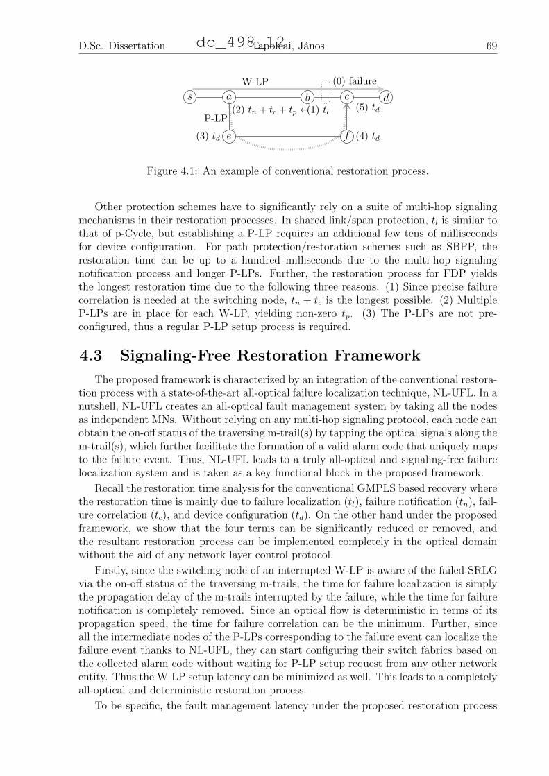
D.Sc. Dissertation Tapolcai, Janos 69
s a
(2) tn + tc + tp ←
b(1) tl
c(5) td
d
e(3) td f (4) td
(0) failureW-LP
P-LP
Figure 4.1: An example of conventional restoration process.
Other protection schemes have to significantly rely on a suite of multi-hop signalingmechanisms in their restoration processes. In shared link/span protection, tl is similar tothat of p-Cycle, but establishing a P-LP requires an additional few tens of millisecondsfor device configuration. For path protection/restoration schemes such as SBPP, therestoration time can be up to a hundred milliseconds due to the multi-hop signalingnotification process and longer P-LPs. Further, the restoration process for FDP yieldsthe longest restoration time due to the following three reasons. (1) Since precise failurecorrelation is needed at the switching node, tn + tc is the longest possible. (2) MultipleP-LPs are in place for each W-LP, yielding non-zero tp. (3) The P-LPs are not pre-configured, thus a regular P-LP setup process is required.
4.3 Signaling-Free Restoration Framework
The proposed framework is characterized by an integration of the conventional restora-tion process with a state-of-the-art all-optical failure localization technique, NL-UFL. In anutshell, NL-UFL creates an all-optical fault management system by taking all the nodesas independent MNs. Without relying on any multi-hop signaling protocol, each node canobtain the on-off status of the traversing m-trail(s) by tapping the optical signals along them-trail(s), which further facilitate the formation of a valid alarm code that uniquely mapsto the failure event. Thus, NL-UFL leads to a truly all-optical and signaling-free failurelocalization system and is taken as a key functional block in the proposed framework.
Recall the restoration time analysis for the conventional GMPLS based recovery wherethe restoration time is mainly due to failure localization (tl), failure notification (tn), fail-ure correlation (tc), and device configuration (td). On the other hand under the proposedframework, we show that the four terms can be significantly reduced or removed, andthe resultant restoration process can be implemented completely in the optical domainwithout the aid of any network layer control protocol.
Firstly, since the switching node of an interrupted W-LP is aware of the failed SRLGvia the on-off status of the traversing m-trails, the time for failure localization is simplythe propagation delay of the m-trails interrupted by the failure, while the time for failurenotification is completely removed. Since an optical flow is deterministic in terms of itspropagation speed, the time for failure correlation can be the minimum. Further, sinceall the intermediate nodes of the P-LPs corresponding to the failure event can localize thefailure event thanks to NL-UFL, they can start configuring their switch fabrics based onthe collected alarm code without waiting for P-LP setup request from any other networkentity. Thus the W-LP setup latency can be minimized as well. This leads to a completelyall-optical and deterministic restoration process.
To be specific, the fault management latency under the proposed restoration process
dc_498_12
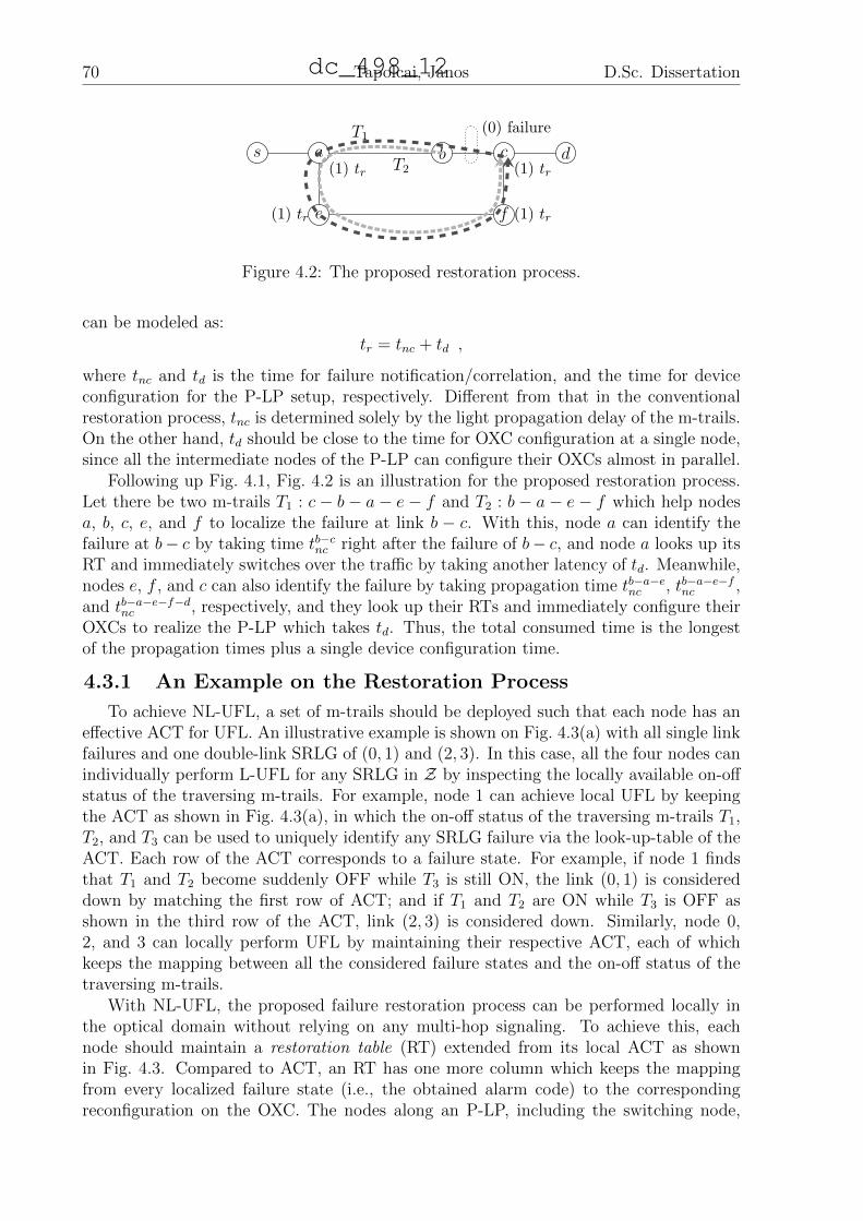
70 Tapolcai, Janos D.Sc. Dissertation
s a(1) tr
b c(1) tr
d
e(1) tr f (1) tr
(0) failureT1
T2
Figure 4.2: The proposed restoration process.
can be modeled as:
tr = tnc + td ,
where tnc and td is the time for failure notification/correlation, and the time for deviceconfiguration for the P-LP setup, respectively. Different from that in the conventionalrestoration process, tnc is determined solely by the light propagation delay of the m-trails.On the other hand, td should be close to the time for OXC configuration at a single node,since all the intermediate nodes of the P-LP can configure their OXCs almost in parallel.
Following up Fig. 4.1, Fig. 4.2 is an illustration for the proposed restoration process.Let there be two m-trails T1 : c− b− a− e− f and T2 : b− a− e− f which help nodesa, b, c, e, and f to localize the failure at link b − c. With this, node a can identify thefailure at b− c by taking time tb−cnc right after the failure of b− c, and node a looks up itsRT and immediately switches over the traffic by taking another latency of td. Meanwhile,nodes e, f , and c can also identify the failure by taking propagation time tb−a−enc , tb−a−e−fnc ,and tb−a−e−f−dnc , respectively, and they look up their RTs and immediately configure theirOXCs to realize the P-LP which takes td. Thus, the total consumed time is the longestof the propagation times plus a single device configuration time.
4.3.1 An Example on the Restoration Process
To achieve NL-UFL, a set of m-trails should be deployed such that each node has aneffective ACT for UFL. An illustrative example is shown on Fig. 4.3(a) with all single linkfailures and one double-link SRLG of (0, 1) and (2, 3). In this case, all the four nodes canindividually perform L-UFL for any SRLG in Z by inspecting the locally available on-offstatus of the traversing m-trails. For example, node 1 can achieve local UFL by keepingthe ACT as shown in Fig. 4.3(a), in which the on-off status of the traversing m-trails T1,T2, and T3 can be used to uniquely identify any SRLG failure via the look-up-table of theACT. Each row of the ACT corresponds to a failure state. For example, if node 1 findsthat T1 and T2 become suddenly OFF while T3 is still ON, the link (0, 1) is considereddown by matching the first row of ACT; and if T1 and T2 are ON while T3 is OFF asshown in the third row of the ACT, link (2, 3) is considered down. Similarly, node 0,2, and 3 can locally perform UFL by maintaining their respective ACT, each of whichkeeps the mapping between all the considered failure states and the on-off status of thetraversing m-trails.
With NL-UFL, the proposed failure restoration process can be performed locally inthe optical domain without relying on any multi-hop signaling. To achieve this, eachnode should maintain a restoration table (RT) extended from its local ACT as shownin Fig. 4.3. Compared to ACT, an RT has one more column which keeps the mappingfrom every localized failure state (i.e., the obtained alarm code) to the correspondingreconfiguration on the OXC. The nodes along an P-LP, including the switching node,
dc_498_12
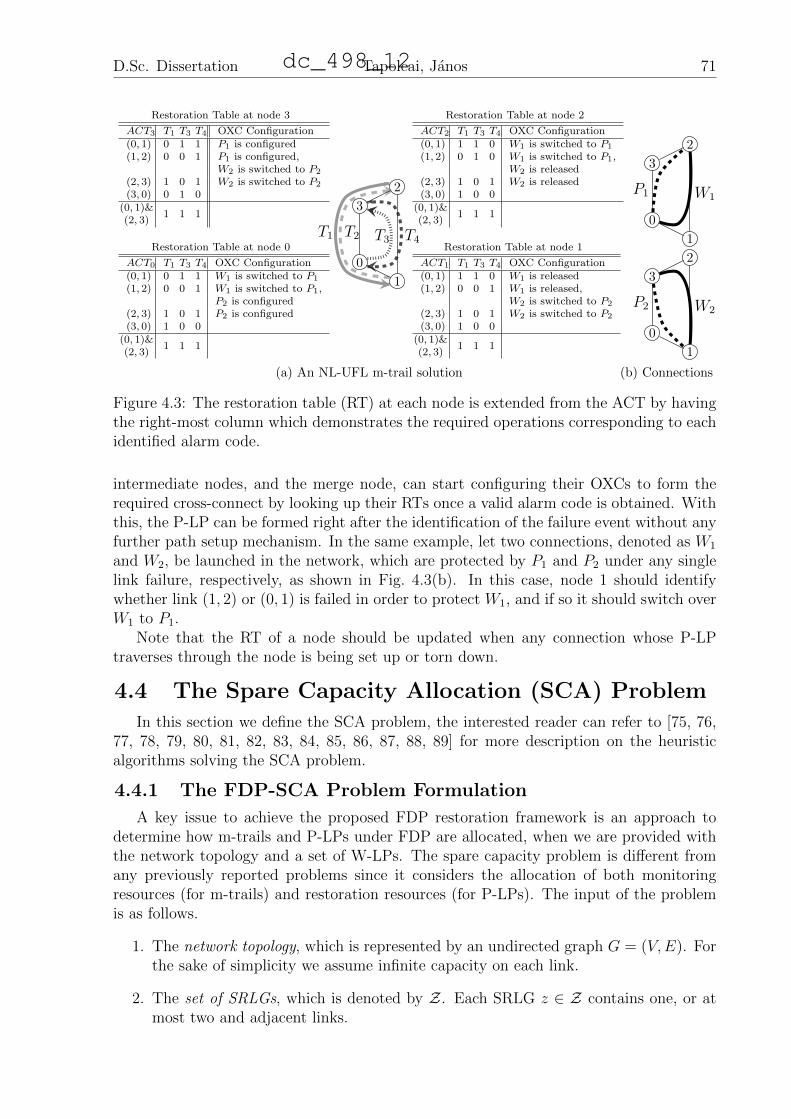
D.Sc. Dissertation Tapolcai, Janos 71
T1 T2 T3 T4
0
1
2
3
Restoration Table at node 1
ACT1 T1 T3 T4 OXC Configuration(0, 1) 1 1 0 W1 is released(1, 2) 0 0 1 W1 is released,
W2 is switched to P2
(2, 3) 1 0 1 W2 is switched to P2
(3, 0) 1 0 0(0, 1)&(2, 3)
1 1 1
Restoration Table at node 2
ACT2 T1 T3 T4 OXC Configuration(0, 1) 1 1 0 W1 is switched to P1
(1, 2) 0 1 0 W1 is switched to P1,W2 is released
(2, 3) 1 0 1 W2 is released(3, 0) 1 0 0
(0, 1)&(2, 3)
1 1 1
Restoration Table at node 0
ACT0 T1 T3 T4 OXC Configuration(0, 1) 0 1 1 W1 is switched to P1
(1, 2) 0 0 1 W1 is switched to P1,P2 is configured
(2, 3) 1 0 1 P2 is configured(3, 0) 1 0 0
(0, 1)&(2, 3)
1 1 1
Restoration Table at node 3
ACT3 T1 T3 T4 OXC Configuration(0, 1) 0 1 1 P1 is configured(1, 2) 0 0 1 P1 is configured,
W2 is switched to P2
(2, 3) 1 0 1 W2 is switched to P2
(3, 0) 0 1 0(0, 1)&(2, 3)
1 1 1
(a) An NL-UFL m-trail solution
P1 W1
0
1
2
3
P2 W2
0
1
2
3
(b) Connections
Figure 4.3: The restoration table (RT) at each node is extended from the ACT by havingthe right-most column which demonstrates the required operations corresponding to eachidentified alarm code.
intermediate nodes, and the merge node, can start configuring their OXCs to form therequired cross-connect by looking up their RTs once a valid alarm code is obtained. Withthis, the P-LP can be formed right after the identification of the failure event without anyfurther path setup mechanism. In the same example, let two connections, denoted as W1
and W2, be launched in the network, which are protected by P1 and P2 under any singlelink failure, respectively, as shown in Fig. 4.3(b). In this case, node 1 should identifywhether link (1, 2) or (0, 1) is failed in order to protect W1, and if so it should switch overW1 to P1.
Note that the RT of a node should be updated when any connection whose P-LPtraverses through the node is being set up or torn down.
4.4 The Spare Capacity Allocation (SCA) Problem
In this section we define the SCA problem, the interested reader can refer to [75, 76,77, 78, 79, 80, 81, 82, 83, 84, 85, 86, 87, 88, 89] for more description on the heuristicalgorithms solving the SCA problem.
4.4.1 The FDP-SCA Problem Formulation
A key issue to achieve the proposed FDP restoration framework is an approach todetermine how m-trails and P-LPs under FDP are allocated, when we are provided withthe network topology and a set of W-LPs. The spare capacity problem is different fromany previously reported problems since it considers the allocation of both monitoringresources (for m-trails) and restoration resources (for P-LPs). The input of the problemis as follows.
1. The network topology, which is represented by an undirected graph G = (V,E). Forthe sake of simplicity we assume infinite capacity on each link.
2. The set of SRLGs, which is denoted by Z. Each SRLG z ∈ Z contains one, or atmost two and adjacent links.
dc_498_12

72 Tapolcai, Janos D.Sc. Dissertation
3. A set of W-LPs denoted as W = W1,W2, . . . ,Wk, where k is the total number ofW-LPs. Each Wj is a path in G between nodes sj and dj for j = 1, . . . , k.
The SCA problem is to minimize the total spare capacity (denoted by M) whileachieving: (i) a feasible solution for NL-UFL m-trail allocation under multi-link SRLGs,and (ii) restoration capacity allocation for FDP. Formally
M =∑e∈E
ue , (4.2)
where ue denotes the spare capacity along link e ∈ E in terms of the number of wavelengthlinks (WLs).
An important feature of the proposed approach is that the spare capacity taken bythe m-trails can be reused by any P-LP. This is a reasonable assumption since both sparecapacity by P-LPs and m-trails are not launched with working traffic during normaloperations. Once there is a failure, all monitoring resources for the m-trails can bereleased and reused by the P-LPs, thanks to NL-UFL which enables all the nodes toinstantly react upon the identified failure. With this, we have:
ue = maxme, pe,
where me denotes the required monitoring resources for the m-trails as
me =∑
1≤j≤b
ITj,e (4.3)
where ITj,e is the trail-link indicator (a.k.a global ACT) which is 1 if the jth m-trail passingthrough link e, and 0 otherwise. And pe denotes the restoration capacity for FDP on linke ∈ E that is formalized as follows.
The Restoration Capacity
For each Wj, 1 ≤ j ≤ k, a set of P-LPs denoted as P zj ,∀z ∈ Zj, is determined such
that they are simple paths with source sj and destination dj while disjoint from each z.Let Wz ⊆ W be a subset of W-LPs, which are the W-LPs possibly interrupted by failurez. Let Zj ⊆ Z be a subset of SRLGs traversed by Wj. The amount of reserved workingcapacity along link e is denoted as qe, ∀e ∈ E; formally qe =
∑1≤j≤k I
Wj,e, where IWj,e is a
working path-link indicator which is 1 if Wj passes through link e, and 0 otherwise. Let
IP,zj,e be a protection path-link indicator which is 1 if P zj traverses e, and 0 otherwise. Let
the restoration capacity along link e in the failure event of z be denoted by pze. We havethe following relation:
pze =∑
1≤j≤k
IP,zj,e −∑
Wj∈Wz
IWj,e
where the term∑
Wj∈Wz IWj,e stands for the free capacity gained by stub release at link eafter the failure event at z which interrupted all Wj ∈ Wz.
The condition for pe to restore every affected W-LP Wj ∈ Wz by failure z is:
pe ≥ maxz∈Zj
pze .
In general, the monitoring resource consumption is determined only by the topologyand SRLGs considered in the problem regardless of the traffic, which serves as a constant
dc_498_12

D.Sc. Dissertation Tapolcai, Janos 73
expense; on the other hand, the amount of restoration resources heavily depends on theamount of working traffic. Thus, when the amount of working capacity increases, moremonitoring resources will be reused due to the increased restoration resource consumption,and gradually all the monitoring resources are reused. We define the monitoring resourcesthat are not shared by any P-LP as monitoring overhead, denoted by
re = max0,me − pe.
The monitoring resources are expected to be completely hidden by P-LPs, provided thatwe have sufficient working capacity in the network, resulting zero monitoring overhead.This is also referred to as the monitoring resource hidden property where all WLs takenby m-trails are also reserved by P-LPs.
4.4.2 FDP Restoration Capacity Allocation
The restoration capacity allocation problem for FDP has been extensively investigatedin the past decades, which is formally called Spare Capacity Placement/Allocation forPath Restoration with stub release. Detailed descriptions can be found in [75, 78, 76], [90,Chapter 6], [91, Chapter 9.5.2] for both ILP formulations and heuristic approaches. Sincewe have positioned our study on a signaling-free FDP-based restoration process via all-optical failure localization, we do not focus on novel FDP restoration capacity allocationschemes; instead, we would adopt state-of-the-art FDP spare capacity allocation schemesfor the proof of concept and facilitation of performance analysis. To be specific, theILP in [91] and Successive Survivable Routing (SSR) algorithm in [78] are implementedin Section 4.6 for comparison with other counterparts as well as for understanding theperformance behaviors under the monitoring resource hidden property, respectively.
4.5 The Monitoring Resource Hidden Property
With the SCA problem formulated in the previous section, we are particularly inter-ested in the monitoring resource hidden property, which defines and quantifies in whatcircumstances the monitoring WLs are all reused by the P-LPs. In other words, thereis no additional resource consumed due to the deployment of the m-trails and thus thespare capacity consumption is the same as that of the conventional FDP which is opti-mal among all the protection schemes. As a first study into the proposed framework, weanalyze the problem under single-link SRLGs in circulant graphs, aiming to gain deeperunderstanding on the performance behaviour of the proposed framework.
4.5.1 Lower Bound on the Spare Capacity
Lemma 16. Let K be a set of links that form a cut in G. The spare capacity along thelinks in K is at least
1
|K| − 1
∑e∈K
qe ≤∑e∈K
pe . (4.4)
Proof. In case link e fails, protection routes must be able to circumvent e via the otherlinks in K, thus the spare capacity along those links is at least qe, formally
qe ≤∑
f∈K,e6=f
pf . (4.5)
dc_498_12

74 Tapolcai, Janos D.Sc. Dissertation
There are |K| such inequalities for 1 ≤ e ≤ |K|. By summing up these inequalities we get∑e∈K
qe ≤∑e∈K
∑f∈K,e6=f
pf = (|K| − 1) ·∑e∈K
pe . (4.6)
Finally, dividing both sides by (|K| − 1) we get Eq. (4.4).
Corollary 4. Let K1, . . . , Kk be a pairwise disjoint cuts. Then
M≥∑
1≤l≤k
∑e∈Kl
qe|K l| − 1
. (4.7)
Corollary 5. Let NG(v) denote the set of links adjacent to node v and ∆v = |NG(v)|
M ≥∑v∈V
∑e∈NG(v)
qe∆v − 1
. (4.8)
As a rule of thumb, the minimal ratio of spare to working capacity can be estimatedby 1/(∆− 1) [75], where ∆ = 2|E|/|V | is the average nodal degree. It was proved for thecase when the working capacity is the same on every link [75]. This can be also deducedfrom Corollary 5 by applying the inequality of arithmetic and harmonic means.
4.5.2 Dominance of Monitoring Resources
With the proposed NL-UFL construction in the Cn(1, 2) topologies, we are interestedin whether and how much monitoring resources can be hidden by restoration resources.Let the average working capacity per link, the average restoration capacity per link, andaverage monitoring capacity per link, be denoted by
q =1
|E|∑e∈E
qe, p =1
|E|∑e∈E
pe, m =1
|E|∑e∈E
me,
respectively. Formally, the dominance of monitoring resources occurs when m ≥ p, whichserves as a sufficient condition that additional monitoring resources are required by FDPon top of the restoration capacity .
Let θ measure the traffic demand as a percentage of s− d pairs that are loaded with aW-LP. For example, θ = 100% means each s−d pair (i.e., |V |(|V |−1)/2) is connected by aW-LP. It is clear that with smaller θ, the dominance of monitoring resources is more likelyto happen. There naturally comes up an interesting question: with a specific topology, forwhich values of θ will make the monitoring resources dominant? Is there a lower boundon θ, say 1%, below which m < p is unconditionally true? In the following theorem weshow that there is no such lower bound on θ in a circulant topology G = Cn(1, 2) undersingle-link SRLGs.
Theorem 16. For any positive θ > 0, there exists a FDP-SCA problem (with topology,SRLG and traffic) where the monitoring resources will never dominate the spare capacity(i.e., m < p).
Proof. We pick the circulant graphs G = Cn(1, 2) as a topology with unit cost along eachlink, and all single link failures for SRLG. Let G = Cn(1, 2) contain a set of nodes denotedas 0, 1, . . . , n−1, and edges denoted as (v, v+1) and (v, v+2), for v = 0, . . . , n−1, where
dc_498_12

D.Sc. Dissertation Tapolcai, Janos 75
the addition is understood modulo n. Let us call the edges (v, v+1) by on-cycle edges andthe rest chordal edges (see also Fig. 2.10). As for the traffic, let G be launched with a set
of shortest-path routed W-LPs denoted asW = W1, . . . ,Wk, such that k ≤ θ · n(n−1)2
. Leth = max5, d1
θe and n = 4h ≥ 20. Nodes s and d are connected with a W-LP along the
shortest path route if s− d ≡ 0 mod h. In this case the number of directed connectionsis k = 3
2n, because each source node s is connected with s+ h, s+ 2h and s+ 3h, where
addition is understood modulo n. Therefore, the total number of directed connections is
θ · n(n− 1)
2= θ · 4 ·max5, d1
θen− 1
2≥ 2(n− 1) ≥ 3
2n = k
Next, we define a set of disjoint cuts K1, . . . , Kn/4, where Ki contains 6 links (v −1, v+1), (v, v+1), (v, v+2) for both v = 2i and v = 2i+n/2. Each cut Ki, i = 1, . . . n/4separates the graph into two equal-size fragments with n
2nodes, thus the number of W-
LPs passing through the cut is at least n, because for each source node s the number ofpossible destination nodes in the other side of the cut is 2, thus there are at least n forwhich s− d ≡ 0 mod h holds.
According to Corollary 4 we haveM≥ 15·n · 6
4n, where 6
4n is the total number of links
in the cuts K1, . . . , Kn/4. Since the number of links is |E| = 2n we have p = M2n
. Accordingto Theorem 7, the total monitoring capacity of the bm-trails is ndlog2 n + 1e + n. Thuswe have m = 1
2(dlog2 n+ 1e+ 1). Therefore, m < p holds when dlog2 n+ 1e+ 1 < 3
10· n
which is always true for n ≥ 20.
It is important to note that although necessary, the dominance of monitoring resourcesis not sufficient for nonzero monitoring overhead.
4.6 Performance Evaluation
4.6.1 Comparison of Signaling-Free Protection Methods
First, a case study is showed to examine the proposed framework in terms of (1)capacity efficiency, (2) restoration time, and (3) computation time. We launched the m-trails to achieve NL-UFL and implemented a FDP scheme (referred to as ”FDP”) as arealization of the proposed framework, which is compared with a couple of signaling-freerestoration schcmes, namely Collaborative Failure Protection (referred to as CFP) andp-Cycle. Both p-cycle and CFP organizes spare capacity into pre-cross-connected cyclesto achieve signaling free protection. CFP can achieve better capacity efficiency by reusingthe released working capacity of the disrupted lightpaths (i.e., stubs). It is achieved in acooperative manner among the failure-aware nodes. We computed the optimal solutionsby implementing and solving the ILP for each of the three schemes, specifically the onein [73], [92] and [91, Chapter 9.5.2] for p-Cycle, CFP, and FDP, respectively, in whichthe same link cost and traffic values were adopted to ensure the experiment environmentscompletely in line with the previous art. We assume the given traffic matrix correspondsto 1 Erlang; each link has 16 WLs, and the W-LPs are shortest-path routed in each case.The results were obtained by solving the ILPs using CPLEX v.11, all with a zero gap tothe optimal. Smallnet [92] topology (10 nodes, 22 edges) is adopted.
Capacity Efficiency
Fig. 4.4 compares the capacity efficiency of the three schemes. It clearly shows thatthe performance of the proposed FDP is dominated by the monitoring resource consump-
dc_498_12

76 Tapolcai, Janos D.Sc. Dissertation
tion by the m-trails when the traffic load is slight, but becomes the most efficient onewhen the traffic load is increased because all the monitoring resource consumption canbe hidden by the spare capacity taken by the P-LPs of the FDP scheme. Note that PDFyields the optimal capacity efficiency among all the protection schemes, and the capacityconsumption by FDP is completely dominated by the PDF spare capacity when the trafficload is heavy enough to hide all the monitoring resource consumption.
Restoration Time
We assume the average physical length of a link is 200km, which requires 1ms for lightto traverse; thus the failure localization and notification delays under FDP is tnl < 20mssince the longest m-trail is no longer than 20 hops. By assuming tp + tc = 10 ms andtd = 20ms, this leads to an overall average restoration time of 50ms. For CFP and p-Cycle, the maximal length of each cycle is 10 hops, which yields tl < 10ms for failurelocalization and notification; however we also have td = 20ms required at the two nodesfor switch fabric configuration and tp + tc = 10, which results in 40ms in total. For CFP,the longest p-Cycle has 7 links, which leads to slightly shorter restoration time than 40ms. Under the specification of the case study, the three schemes lead to very similarrestoration time.
Computation Time
The computation time was 39, 004sec, 17.22sec, and 3.94sec for CFP, p-Cycle, andFDP, respectively. The proposed FDP has the best computation efficiency.
Under Multi-Link SRLGs
We have adopted the problem instance in [74] for comparison, which is, to the best ofour knowledge, the only previously reported study that provides an ILP for static multi-link SRLG p-cycle design. Note that all the other studies for multi-link SRLGs usingp-cycles have focused on reconfiguration, rerouting, and dynamic reconfiguration of sparecapacity, which do not fit into the targeted scenario. The NSF network (14 nodes, 22 links)topology is used for all single-link and double-link SRLGs. P-cycle requires 965 bandwidthunit while NL-UFL&FDP 302. This clearly shows that the proposed NL-UFL&FDPapproach can gain even more advantage when multi-link SRLGs are considered. Theaverage length of m-trails is 20 links, while the maximum is 26 links, which still results sub50ms restoration time for every single and double failure with NL-UFL&FDP approach.
4.6.2 Monitoring Resources Hidden
We have seen that the proposed approach is outperformed by its counterparts when theworking traffic load is small, but will become much more efficient when the number of W-LPs increases, and the monitoring resources can be completely hidden by the restorationcapacity for FDP. Therefore, we claim that the proposed approach can achieve the samecapacity efficiency as conventional FDP provided the network is loaded with sufficientlylarge working capacity. This subsection provides extensive simulation results in a widerange of network topologies and SRLG densities, so as to gain deeper understanding onthe monitoring resource hidden property under the proposed restoration framework.
The randomly generated planar graphs are classified according to parameter g, whichis the length of the longest inner face contained in the graph. Clearly, graphs withsmaller values of g are considered more densely meshed; and in the generated graphs,the average nodal degree of each graph ranges from 5.4 (for g = 3) to 2.76 (for g = 7).
dc_498_12

D.Sc. Dissertation Tapolcai, Janos 77
0
1
2
3
4
5
6
7
1 2 3 4 5 6 7 8
WL
per
lin
k
Erlang
FDPM-trailP-cycle
CFP
Figure 4.4: WLs fper link on Smallnet.
0
5
10
15
20
25
0 50 100
Ave
rage
Cost
% of s− d pairs
f = 0f = 10f = 30f = 50f = 90
(a) COST266 network
0
1
2
3
4
5
6
7
8
0 50 100
Ave
rage
Cos
t
% of s− d pairs
g = 3g = 4g = 5g = 6g = 7
(b) Random networks with f = 0
Figure 4.5: Average monitoring overhead.
See also Fig. 3.5 for example network topologies with different g. Besides, the COST266European reference network (37 nodes, 57 links) is also used [93]. We adopted SRLGs withsingle link and double adjacent links, and the SRLG density considered in the problem isparameterized by a double failure density parameter, denoted by f , which indicates thefraction f of all double adjacent link SRLGs under consideration.
We evaluate the resource consumption in the proposed framework by increasing theworking traffic, which is defined as the percentage of s− d pairs that are interconnectedby a W-LP (i.e., θ). Let every W-LP and m-trail take a single wavelength of bandwidth(i.e., a single WL). The ILP in [91] was no longer used here due to the huge computationcomplexity; instead, we adopted SSR [78] that sequentially allocates P-LPs for each W-LP. SSR iteratively launches Dijkstra’s shortest path algorithm to find disjoint backuppaths with each SRLG involved in W-LP one at a time using the latest spare capacityinformation.
Fig. 4.5(a) and (b) show the average monitoring overhead, i.e.,
1
|E|·∑e∈E
max0,me − pe,
as θ is increased from 0% to 100%. It meets our expectation that as the percentage of
dc_498_12
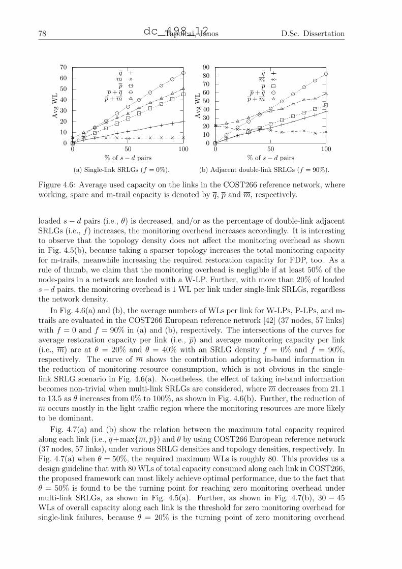
78 Tapolcai, Janos D.Sc. Dissertation
0
10
20
30
40
50
60
70
0 50 100
Avg
WL
% of s− d pairs
qmp
p+ qp+m
(a) Single-link SRLGs (f = 0%).
0
10
2030
40
50
6070
80
90
0 50 100
Avg
WL
% of s− d pairs
qmp
p+ qp+m
(b) Adjacent double-link SRLGs (f = 90%).
Figure 4.6: Average used capacity on the links in the COST266 reference network, whereworking, spare and m-trail capacity is denoted by q, p and m, respectively.
loaded s− d pairs (i.e., θ) is decreased, and/or as the percentage of double-link adjacentSRLGs (i.e., f) increases, the monitoring overhead increases accordingly. It is interestingto observe that the topology density does not affect the monitoring overhead as shownin Fig. 4.5(b), because taking a sparser topology increases the total monitoring capacityfor m-trails, meanwhile increasing the required restoration capacity for FDP, too. As arule of thumb, we claim that the monitoring overhead is negligible if at least 50% of thenode-pairs in a network are loaded with a W-LP. Further, with more than 20% of loadeds−d pairs, the monitoring overhead is 1 WL per link under single-link SRLGs, regardlessthe network density.
In Fig. 4.6(a) and (b), the average numbers of WLs per link for W-LPs, P-LPs, and m-trails are evaluated in the COST266 European reference network [42] (37 nodes, 57 links)with f = 0 and f = 90% in (a) and (b), respectively. The intersections of the curves foraverage restoration capacity per link (i.e., p) and average monitoring capacity per link(i.e., m) are at θ = 20% and θ = 40% with an SRLG density f = 0% and f = 90%,respectively. The curve of m shows the contribution adopting in-band information inthe reduction of monitoring resource consumption, which is not obvious in the single-link SRLG scenario in Fig. 4.6(a). Nonetheless, the effect of taking in-band informationbecomes non-trivial when multi-link SRLGs are considered, where m decreases from 21.1to 13.5 as θ increases from 0% to 100%, as shown in Fig. 4.6(b). Further, the reduction ofm occurs mostly in the light traffic region where the monitoring resources are more likelyto be dominant.
Fig. 4.7(a) and (b) show the relation between the maximum total capacity requiredalong each link (i.e., q+maxm, p) and θ by using COST266 European reference network(37 nodes, 57 links), under various SRLG densities and topology densities, respectively. InFig. 4.7(a) when θ = 50%, the required maximum WLs is roughly 80. This provides us adesign guideline that with 80 WLs of total capacity consumed along each link in COST266,the proposed framework can most likely achieve optimal performance, due to the fact thatθ = 50% is found to be the turning point for reaching zero monitoring overhead undermulti-link SRLGs, as shown in Fig. 4.5(a). Further, as shown in Fig. 4.7(b), 30 − 45WLs of overall capacity along each link is the threshold for zero monitoring overhead forsingle-link failures, because θ = 20% is the turning point of zero monitoring overhead
dc_498_12

D.Sc. Dissertation Tapolcai, Janos 79
0
20
40
60
80
100
120
0 25 50
Max
WL
% of s− d pairs
f=0f=10f=30f=50f=90
(a) COST266 network
0
20
40
60
80
100
120
0 25 50
Max
WL
% of s− d pairs
g = 3g = 4g = 5g = 6g = 7
(b) Random networks with f = 0
Figure 4.7: Maximum overall capacity in WLs.
under single-link SRLGs, as shown in Fig. 4.5(b).
dc_498_12

Chapter 5
IP Fast ReRoute
5.1 Introduction
Transporting delay and loss sensitive traffic in the Internet has become an importantrequirement in the last few years. At the moment the IP protocol suite is not yet readyto fully support multimedia streams due to various reasons, one of which is slow responseto failures. Recovery with current Interior Gateway Protocols (IGPs) is in the order ofhundreds of milliseconds [94], typically beyond what is tolerable to a multimedia stream.Similar is the case of MPLS networks that rely on LDP for label exchange, as LDP isdependent on the IGP for routing. Therefore, the IETF defined a framework called IPFast ReRoute (IPFRR [95]), for native IP protection in order to reduce failure reactiontime to tens of milliseconds in an intra-domain, unicast setting.
IPFRR is based on two principles: local rerouting and precomputed detours. Localrerouting means that only routers directly adjacent to a failure are notified of it, whicheliminates one of the most time-consuming steps of IGP-based restoration: global floodingof failure information. Additionally, IPFRR mechanisms are proactive in that detoursare computed, and installed in the forwarding engine, long before any failure occurs.Thus, when a failure eventually shows up, routers are able to switch to an alternate pathinstantly. Once alternate next-hops are active, traffic flows undisrupted bypassing thefailed component, letting the IGP to converge in the background.
This chapter deals with two specifications for IPFRR, namely the Loop-Free Alternates(LFA) and Protection Routing (PR). The former is the only standardized and readilyavailable IPFRR technology, while the latter is a more theoretic framework as it requiresa centralized unit that controls the forwarding table at each router but it still can beimplemented with OpenFlow routers.
5.2 Loop Free Alternates
A basic specification for IPFRR is Loop-Free Alternates (LFA, [96]). When connec-tivity to some next-hop is lost, all traffic that would have used the unreachable next-hopis passed on to an alternate next-hop, called a Loop Free Alternate, that still has a pathto the destination that is unaffected by the failure. LFA is simple, it can be realizedwith straightforward modifications to current IGPs, and deployment is easy thanks tothe fact that it does not require support from other routers. On the other hand, LFAsdo not always protect both link and node failures at the same time and may also lead totemporary loops when multiple simultaneous failures show up. But the major problem is
80
dc_498_12

D.Sc. Dissertation Tapolcai, Janos 81
that often not all routers have LFAs to all other routers, which means that certain failurepatterns are impossible repair rapidly.
Unfortunately, complete IP-level local protection is difficult due to the IP’s destination-based forwarding paradigm. As only adjacent routers are aware of a failure, remoterouters do not know whether an arriving packet is traveling on its shortest path or itis already on a detour and so exceptional forwarding should be applied. Without beingable to differentiate between these two cases, local IP protection can never attain 100%failure coverage1. Most IPFRR proposals, therefore, either change IP’s destination-basedforwarding [97, 98, 99] or introduce some forms of signaling to indicate that a packet is ona detour. Some call for out-of-band failure signaling [100], others use invaluable extra bitsin the IP header [101, 102] or add special information to it for in-band signaling [103],and still others propose to mark detours by tunneling [104, 105, 106]. While modernrouters can handle tunneled packets at wire speed, tunneling needs additional addressmanagement [107, 106] and, if the additional IP header does not fit into the MTU, cancause packet fragmentation and time-consuming reassembly at the tunnel endpoint. Itseems, therefore, that the price for IP-level local protection, capable to handle all possiblefailure cases, is considerable added complexity and management burden, modifications tothe essential IP infrastructure, and the breaking of the incremental deployment path.
It is, therefore, no wonder that today LFA is the only standardized and readily avail-able IPFRR technology. At least two major router vendors are offering LFA-based IPFRRsupport out of the box [108, 109], and other vendors are expected to follow suit. Conse-quently, operators in need for improving network resilience are now facing the questionwhether to deploy LFA, and this decision depends crucially on the extent to which LFAcan protect failures in the particular topology. We intend to assist making this decision.
Even though thorough, simulation-based reports are available [110, 111, 112, 113, 114],a deep understanding of how certain network characteristics affect LFA failure coverageis still missing. Thus, in this section our focus is on the graph topological ingredientsneeded for good LFA protection. In this regard, our work is a sequel to [115], wherethe authors study to what extent IP’s destination-based forwarding permits protectionrouting, and [116] presenting a similar study for the O2 scheme. As we find that LFAfailure coverage strongly depends on the topology as well as on the link costs, we studythe effects of both separately.
Existing proposals modify standard IP forwarding in some way to achieve full protec-tion. Why not choose the other way around? That is, instead of bending IP to providefull protection in all networks, paying huge price in complexity and deployability, whynot bend the network topology itself so that even LFA can guarantee full protection?We study this question in the first part of the chapter. We show real networks whereby adding just two or three new links full LFA protection can be attained. This mightbe an acceptable price for an operator to take the easy deployment path. In some cases,however, our analysis reveals that full LFA protection can only be achieved at the cost of asubstantial topology redesign, which is a clear indication to choose alternative protectionschemes [81]. At the least, such an analysis can be instructive in the next regular networkupgrade cycle.
1One can easily prove this claim formally, taking the example of a ring with at least 4 nodes.
dc_498_12

82 Tapolcai, Janos D.Sc. Dissertation
a
b
c
d
e
f
g
6
3
3
2
5
8
10
3
6
2
Figure 5.1: A sample weighted network topology.
5.2.1 An Example on Loop Free Alternates
We demonstrate LFA through an example. Consider the network depicted in Fig. 5.1and suppose that router d wishes to send a packet to router f . The next-hop of d alongthe shortest path towards f starts for c. If, however, link (d, c) fails, then d needs tofind an alternative neighbor to pass on the packet. It cannot send the packet to, say, b,as b’s shortest path to f goes through itself, so b would send the packet back causing aloop (remember that in IPFRR, routers not immediately adjacent to a failure do not getnotified of it). Instead, it needs to find a neighbor that is closer to the destination thanthe length of the route from the neighbor through itself. This relation can be expressedas follows:
dist(n, d) < dist(n, s) + dist(s, d) , (5.1)
where s is the actual source node, d is the node the packet is destined to, n is a neighborof s other than the failed next-hop and dist(x, y) denotes the length of the shortestx → y path. A neighbor fulfilling (5.1) is called a link-protecting Loop Free Alternate(LFA). For instance, a is a link-protecting LFA for node d towards node f as dist(a, f) <dist(a, d) + dist(d, f).
Many alternative LFA types exist. For instance, g is also an LFA for d towards f ,but it also protects against the failure of node c, so it is a node-protecting LFA. It isalso a downstream neighbor, as it is closer to f than d, as well as a per-link LFA for thelink (d, c) as it protects all the nodes reachable by d through (d, c). For a full taxonomy,see [96, 113, 114].
5.2.2 Model
We model the network topology by a simple, undirected weighted graph G = (V,E).Let E denote the complement of the edge set. Let the cost of edge (i, j) be c(i, j). Forsimplicity, we assume that (i) edges are bidirectional and point-to-point; (ii) costs aresymmetric; and (iii) each node has a well-defined next-hop towards each destination. Thismeans that if multiple shortest paths are available to a destination, then one is chosenarbitrarily.
In this section we limit our attention to single link failures exclusively. As simplelink-protecting LFAs safeguard against just this type of failures and they contain all theother LFA types as special cases, we do not treat those henceforth. Consequently, weshall usually assume that the graph describing the network is 2-edge-connected, which isthe minimum topological requirement for being able to repair every possible link failure.
dc_498_12

D.Sc. Dissertation Tapolcai, Janos 83
5.2.3 Problem Definition
Definition 2. Consider an undirected, weighted graph G = (V,E). For each d ∈ V ,define a relation (≺d) on V as follows: let u ≺d v if at least one shortest path from v to dgoes through u. Let u d v if either u ≺d v or u = v. Finally, put u ≺d v if u and v arenot ordered by (d).
In Fig. 5.1, for instance, d f b but d b b, and a ≺f d.The relation (d) defines a partial order on V , since it is reflexive, transitive and
antisymmetric. The partially ordered set (V,d) is called the d-poset. Each d-poset hasexactly one lower bound: d. We say that some u ∈ V is an ancestor (descendant) of somev ∈ V in the d-poset if u ≺d v (u d v, respectively). Additionally, a parent (child) is aneighboring ancestor (descendant). By assumption, if a node has multiple parents, thenone is assigned as next-hop arbitrarily.
Using this model, we redefine (5.1) as follows:
Definition 3. For some s ∈ V and d ∈ V , a neighbor n ∈ V of s that is not the next-hopis a link-protecting LFA (simply LFA, henceforth) if s d n.
Simply put, n is an LFA if no shortest path from n to d passes through s. Hence,no loop will arise if a packet destined to d is handed by s to n instead of its primarynext-hop. Note that the condition s d n means that either s ≺d n or s d n.
From the above discussion, it is clear that in general networks not all nodes have LFAprotection to every other node [110, 111, 112, 113, 114]. To measure the LFA failurecoverage η(G) in a weighted graph G, we adopt the simple metric from [96]:
η(G) =#LFA protected (s, d) pairs
#all (s, d) pairs
5.2.4 Bounds on LFA coverage
Next, we present simple lower and upper bounds on LFA coverage. Our bounds arebased on the following idea. The shortest path tree to some destination d can contain onlyn−1 edges, and all the remaining edges can be used for providing LFAs to their endpoints.In particular, an out-of-tree edge provides at most 2 LFAs (either node-protecting or link-protecting or both), and at least 1 link-protecting LFA towards d.
Let ∆ denote the average node degree in G and let ∆max be the maximum degree.It is immediate that, ∆ ≥ 2(|V |−1)
|V | for any connected graph, since the sparsest connected
graphs are trees for which ∆ = 2(|V |−1)|V | . A ∆-regular graph is a graph in which all nodes
are of constant degree ∆. An even (odd) ring is a cycle graph with an even (odd) numberof nodes. Rings are the smallest-degree 2-connected regular graphs (in particular, ∆ = 2).
In [12] the following lemma was proved
Lemma 17. For an even ring with |V | > 2 and uniform costs: η(G) = 1|V |−1
. For an odd
ring with |V | > 2 and uniform costs: η(G) = 2|V |−1
.
Theorem 17. For any connected simple graph G with |V | > 2:
η(G) ≤ |V ||V | − 1
(∆− 2) +2
|V | − 1.
dc_498_12

84 Tapolcai, Janos D.Sc. Dissertation
Proof. We observe that an edge not contained in the shortest path tree rooted at somed provides at most 2 link-protecting LFAs towards d (when the edge lies between twobranches of the tree), while on-tree edges do not create any LFA. Since the number ofout-of-tree edges is exactly |E| − (|V | − 1), at most 2(|E| − |V |+ 1) = |V |∆− 2|V |+ 2 =|V |(∆− 2) + 2 nodes can have LFA to d. Taken the sum over all nodes and dividing bythe number of source-destination pairs gives
η(G) ≤ |V |(|V |(∆− 2) + 2)
|V |(|V | − 1)=|V ||V | − 1
(∆− 2) +2
|V | − 1.
The Lemma is non-trivial for 2(|V |−1)|V | ≤ ∆ < 3. For trees, in particular, we obtain
η(G) ≤ 0, which implies that the Lemma is tight for trees over arbitrary link costs. It istight for uniform cost odd rings as well, for which we obtain η(G) ≤ 2
|V |−1according to
Lemma 17.What the above Lemma in essence says is that in large sparse graphs LFA-coverage
is upper bounded by the average node degree: η(G, c) ≤ ∆ − 2. In the course of ournumerical evaluations, we found that this relation is present in most real-world networksas well (see later).
The next Lemma gives a lower bound on the LFA coverage. Note, however, that theresult concerns link-protecting LFAs exclusively.
Theorem 18. For any connected simple graph G with |V | > 2:
η(G) ≥ |V ||V | − 1
∆2− 1
∆max − 1+
1
(|V | − 1)(∆max − 1).
Proof. Again, exactly |V | − 1 nodes are contained in the shortest path tree of d, and anout-of-tree edge (of which we have |E| − |V | + 1) can provide at least one LFA towardsd: (i) if the edge is inside a single branch of the shortest path tree, then it provides LFAfrom the upstream to the downstream; (ii) if the edge lies between two branches, it stillcreates at least one link-protecting LFA (in fact, it creates two), but it might not createany node-protecting LFA at all. In consequence, there are |E| − |V |+ 1 out-of-tree edges
that are incident to at least |E|−|V |+1∆max−1
=|V |( ∆
2−1)+1
∆max−1nodes providing a link-protecting LFA
towards d (the term ∆max − 1 is because every node has at least one in-tree edge, soonly the rest count as out-of-tree edges). Taking the sum over all nodes and dividing by|V |(|V | − 1) gives the required result.
The most important message here is that LFA coverage increases with ∆, that is, thedenser the network the higher the link-protecting LFA coverage.
Corollary 6. For a ∆-regular graph R∆ on |V | nodes:
η(R∆) ≥ 1
2− 1
2
|V | −∆− 1
(|V | − 1)(∆− 1).
This gives η(R2) ≥ 1|V |−1
and η(R3) ≥ 14
+ 34
1|V |−1
> 14. From this, we conclude that
the lower bound of Lemma 18 is tight for even rings. One easily sees that it is tight fortrees as well.
dc_498_12

D.Sc. Dissertation Tapolcai, Janos 85
We have seen that LFA coverage fundamentally depends on the average node degree.This raises the question whether we can find graphs of low degree with 100% LFA coverage.We found that the 2-connected graph with the smallest possible average degree that canstill be fully protected using LFA is the 3-ring C3. Every other 2-connected graph withcomplete LFA coverage has average degree higher than 2. By Lemma 17, η(C3, c) = 1which is attained when c is uniform, and one easily sees that η(C3, c) is the only 2-connected graph of average degree ∆ = 2 with this property. Graphs with ∆ < 2 cannothave full protection because such graphs contain at least one node with degree 1 whosesingle outgoing link can never be protected. On the other hand, larger 2-connected graphswith ∆ = 2 are all ring topologies, and rings can only have full LFA coverage if n = 3(again, by Lemma 17).
5.2.5 The LFA Topology Extension Problem
The conditions for full LFA coverage turn out to be somewhat restrictive, suggestingthat only special topologies admit full protection. Indeed, practical studies show that incommon networks LFA coverage is usually in the order of 50-90% [110, 111, 112, 113, 114].There are essentially three approaches to increasing LFA coverage: changing link costs[14, 117], changing the topology [12, 13], or doing both.
Next we focus on the question how to extend the network with new links (e.g., by leas-ing additional capacity, provisioning new virtual links, or deploying new fibers) to improveLFA coverage, and we shall recur to manipulating costs only if improvement cannot beachieved otherwise. The practical reason behind it is that in many operational networksedge costs are deliberately optimized for the purposes of load-balancing, reducing delayand improving resiliency [118], or to obviate equal-cost paths in order to eliminate packetre-ordering, unwanted packet fragmentation [119], etc. Modifying costs would destroycarefully engineered shortest paths and this would make deploying LFA less attractive tooperators.
We study the impacts of the graph topology and edge costs separately.
LFA Graph Extension: Uniform Link Costs
In this section, we ask how to add edges to a graph to achieve full LFA coverage,provided that both the edges originally existing in the graph and the edges we add havethe same cost. Obviously, we want to do this with the fewest new edges possible. Considerthe problem statement:
Definition 4. LFA graph extension problem in the uniform cost case (minLFAu): Givena simple, undirected graph G = (V,E) with uniform edge costs c on all edges and aninteger l, is there a set F ⊆ E with |F | ≤ l and ∀(u, v) ∈ F : c(u, v) = c so that forG′ = (V,E ∪ F ) we have η(G′) = 1?
Next, we turn to the characterization of networks with perfect LFA coverage. Herein,we concentrate on the uniform cost case, when shortest path routing boils down to min-hop routing.
Observation 1. Consider an undirected graph G with uniform edge costs. Now, η(G) = 1,if and only if each node has an LFA towards each of its neighbors.
Easily, if all neighbors are protected, then all nodes in the graph are protected as wellsince these are reached through the neighbors. The other way around: if η(G) = 1 then,
dc_498_12

86 Tapolcai, Janos D.Sc. Dissertation
evidently, all neighbors must be protected. We will use the following theorem taken from[12].
Lemma 18. Consider an undirected, simple graph G = (V,E) with uniform costs. Now,η(G) = 1, if and only if each edge is contained in at least one triangle (cycle of length 3).
Proof. First, we show that if all (u, v) ∈ E are contained in a triangle, then η(G) = 1.Let some triangle containing (u, v) be u − v − w. One easily sees that u v w, as it isthe direct path through edge (w, v) that is the shortest (min-hop) path from w to v, andw → u → v is strictly longer than that. Thus, w is an LFA for u towards v protectingedge (u, v), and the claim then follows from Observation 1.
To see the reverse direction, we prove that if η(G) = 1, then every edge is containedin a triangle. If η(G) = 1, then for each (u, v) ∈ E node u has an LFA towards v. Letthis be w. Easily, (u,w) ∈ E. We only need to show that (w, v) ∈ E as well to have atriangle. Indirectly, if (w, v) /∈ E, then u v w, which contradicts the assumption that wis an LFA.
Lemma 18 implies that complete graphs, chordal graphs and maximal planar graphshave full LFA coverage in the uniform cost case.
Note that adding uniform cost edges to a uniform cost graph necessarily changes theshortest paths between some of the nodes. This is because at least the nodes connectedby the new edge will use it to reach each other, instead of whatever shortest path they hadbefore. Hence, the requirement that shortest paths be invariant to LFA graph extensioncannot be met when solving minLFAu.
Theorem 19. The LFA graph extension problem in the uniform cost case (minLFAu) isNP-complete.
Definition 5 (SP5, [120]). Minimal set cover problem (minSC): Given a bipartite graphG′ = (A ∪ B,C) and a positive integer k, is there a set of nodes Bc ⊆ B with |Bc| ≤ k,such that every node in A has a neighbor in Bc?
We make the following trivial assumptions: (i) each node a ∈ A is connected to atleast two nodes in B (otherwise covering a is trivial); (ii) |B| ≥ 3; and (iii) |A| ≥ 2.
Proof. Instead of solving minLFAu directly, we use Lemma 18. Consider the definition:
Definition 6. Minimal triangular problem (minTR): Given a graph G = (V,E) and apositive integer l, is it possible to add at most l edges to G so that every edge is containedin a triangle?
Easily, minTR is solvable for l if and only if minLFAu is also solvable for l. Hence,proving that minTR is NP-complete will yield the required result. MinTR is in NP,since a nondeterministic algorithm needs to guess the set of edges F with |F | ≤ l and apolynomial time algorithm can verify if every edge is part of a triangle. To prove thatminTR is indeed NP-hard, we (Karp-)reduce minSC to minTR: given a minSC instancewith a bipartite graph G′ = (A ∪ B,C) and an integer k, our task is to define an inputgraph G = (V,E) for minTR that is solvable with at most k edges, if and only if theminSC instance is solvable with at most k nodes.
Construct G = (V,E) as follows: let V = A1∪A2∪B∪s, |V | = 2|A|+|B|+1. Denotethe nodes in V by a1
i ∈ A1, a2i ∈ A2, bj ∈ B and s, respectively, where i = 1, . . . , |A| and
j = 1, . . . , |B|. Additionally, let E = E1 ∪ E2 ∪ E3 where:
dc_498_12

D.Sc. Dissertation Tapolcai, Janos 87
E1: (a1i , bj) and (a2
i , bj) if (ai, bj) ∈ C,
E2: (s, a1i ) and (s, a2
i ) for i = 1, . . . , |A|,
E3: (bj, bl) for all j = 1, . . . , |B|, l = 1, . . . , |B| and j 6= l.
A minSC instance and its transformation are given in Fig. 5.2.We say that an edge is protected if it is part of a triangle, unprotected otherwise.
We make the following observations: edges in E1 are protected because of assumption(i), similarly edges in E3 are also protected because of (ii), while edges in E2 are allunprotected. The idea is that in order to protect all edges in E2 we need to add (s, bj) :bj ∈ B edges, called cover edges henceforth. Each such (s, bj) cover edge, when added,protects the (s, a1
i ), (s, a2i ) ∈ E2 edges for all ai ∈ A nodes adjacent to bj in G′. Thus, we
get a minimal cover of G′ exactly when all edges in E2 become protected.To conclude the proof we need to show that (a) if G′ can be covered with k nodes from
B, then we can identify k edges to be added to G so that every edge becomes protected;and (b) if k edges are added to G so that every edge becomes protected, then we canidentify a k node subset of B that covers every node in A.
(a) Let Bc ⊆ B be a cover in G′ with |Bc| ≤ k. Add edges (s, bl) : ∀bl ∈ Bc to E.Then, since Bc is adjacent to every node in A1 and A2 (due to it being a cover), everyedge in E2 becomes protected. This is because, the edges (s, axi ) ∈ E2, (axi , bl) ∈ E1 and(s, bl) make up a triangle; where axi is adjacent to bl and x = 1, 2.
(b) Suppose that there is a set of cover edges F ′ such that F ′ = (s, bj) : bj ∈ B′ ⊆ Band B′ is adjacent to every node in A1 and A2. Then, by the above reasoning, F ′ can beconverted to a set cover. Let F ∈ E be a set of edges which, when added to G, protectall edges. First, we add all cover edges of F to F ′. Now, suppose that some edges inF are not cover edges. F does not contain edges of the form (bi, bj) : bi, bj ∈ B and(s, axi ) : axi ∈ A1 ∪ A2, since these all exist in E. Edges (axi , bj) : axi ∈ A1 ∪ A2, bj ∈ Bcan be dropped from F , as these do not protect any unprotected edge. What remains areedges of the type (axi , a
zj) : axi , a
zj ∈ A1 ∪ A2. Let us call these cross edges. Furthermore,
call a node axi ∈ A1 ∪A2 protected if the edge (s, axi ) is protected. We shall convert crossedges to cover edges before adding to F ′. Clearly, we need to consider only those crossedges where both a1
i ∈ A1 and a2i ∈ A2 are protected by a cross edge, otherwise a cover
edge in F ′ already covers both a1i and a2
i . Let A′1 ⊆ A1 and the “opposite nodes” A′2 ⊆ A2
be the set of these nodes. Since one cross edge can protect at most two nodes, there are atleast |A′1| cross edges protecting A′1 and A′2, and these are trivially substituted by exactly|A′1| cover edges: for each a1
i ∈ A′1 choose a neighbor bj ∈ B and add the cover edge (s, bj)to F ′. This will protect a2
i ∈ A′2 too. Finally, all nodes B′ are adjacent to every node inA1 and A2, which completes the proof.
LFA Graph Extension: Weighted Graphs
In contrast to uniform cost graphs, where we could not solve the LFA graph extensionproblem without changing some shortest paths, in weighted graphs we can. If an edgewith sufficiently large cost is added to the graph, then shortest paths remain intact whileLFA coverage may improve. Here, and in the rest of this chapter, “sufficiently large” willgenerally mean “larger than the length of the longest shortest path”.
Definition 7. LFA graph extension problem in the weighted case (minLFAw): Given asimple, undirected, weighted graph G = (V,E) and an integer l, is there a set F ⊆ E with
dc_498_12

88 Tapolcai, Janos D.Sc. Dissertation
a1
a2
a3
an
b1
b2
b3
b4
bm
(a) G′
a11
a12
a13
a1n
a21
a22
a23
a2n
b1
b2
b3
b4
bm
s
(b) G
Figure 5.2: A minSC instance (a) and the converted graph (b).
a1
a2
a3
an
s
b1
b2
b3
b4
bm
2
1 3
4
(a) G = (V,E)
1
1
1
1
d
3
3
3
3
3
(b) d = s
d
2
2
2
1
2
2
4
4
4
(c) d ∈ A
2
4
2
4
3
d
3
3
3
3
(d) d ∈ B
Figure 5.3: The converted graph topology and link costs. Fig. (a) depicts the graph andFig. (b), (c) and (d) give the shortest paths and distances with different choices of thedestination d.
|F | ≤ l and properly chosen costs, so that for G′(V,E ∪ F ) we have η(G′) = 1 and theshortest paths in G coincide with the shortest paths in G′?
Next we characterize the complexity of minLFAw.
Theorem 20. The LFA graph extension problem for the weighted case (minLFAw) isNP-complete.
Proof. The minLFAw problem is in NP, since it was formulated as an ILP in Section 5.2.5.To prove that it is NP-hard, we again reduce minSC to minLFAw (see Definition 5): givena minSC instance with a bipartite graph G′ = (A∪B,C) and an integer k, our task is todefine an input graph G = (V,E) for minLFAw, so that minLFAw is solvable by addingat most k edges if and only if minSC is solvable with at most k nodes.
Let us construct G = (V,E) as follows: V = A ∪B ∪ s and E = E1 ∪E2 ∪E3 ∪E4
where
E1: (s, ai) with cost 1 for each i = 1, . . . , |A|,
E2: (ai, bj) with cost 2 for each (ai, bj) ∈ C,
E3: (bj, bl) with cost 3 for all j = 1, . . . , |B|, l = 1, . . . , |B| and j 6= l,
E4: (ai, aj) with cost 4 for all i = 1, . . . , |A|, j = 1, . . . , |A| and i 6= j.
dc_498_12

D.Sc. Dissertation Tapolcai, Janos 89
Fig. 5.3a shows the converted graph for the same minSC instance we used in theprevious proof (see Fig. 5.2a).
The idea here is that we embed G′ into G and, by carefully choosing the edge costs,we ensure that achieving perfect LFA coverage in G precisely solves the minSC instanceon G′. More formally, we show that some Bc ⊆ B is a cover, if and only if η(G′′) = 1where G′′ = (V,E ∪F ) for some set of edges F : (s, b) : b ∈ Bc of sufficiently large cost.We discuss the LFA coverage for different destinations separately.
1. d = s: As one easily checks in Fig. 5.3b, each node has an LFA towards destinations. Nodes in A provide LFA for each other as they are not ordered in the d-poset and|A| ≥ 2 by assumption (iii). Using (ii), one easily shows that nodes in B also provideLFA for each other.
2. d ∈ A: All nodes in A \ d have an LFA towards d, since they are not orderedin the d-poset and |A| ≥ 2 due to (iii) (see Fig. 5.3c). Similarly, each b ∈ B has an LFAfrom some other node in B. This leaves us with the single node s that does not have anLFA to d. This is because all of its neighbors are in A, but d is its next-hop so it can notbe used as an LFA and all other nodes in A are its children. Nodes not connected to d cannot provide an LFA to s either, since these are all its descendants. What remains are theneighbors of d. So, we have to add an edge (s, bj) for some (d, bj) ∈ C with sufficientlylarge cost to protect edge (s, d).
3. d ∈ B: First, each b ∈ B is protected due to (ii). Second, each a ∈ A that isa neighbor of d is protected by some neighbor b ∈ B \ d. Such neighbor exists dueto (i). Similarly, each a ∈ A that is not a neighbor of d is protected by some neighborb ∈ B \ d, which again exists due to (i). Again, node s remains without an LFA to d.However, at this point there already is at least one edge (s, bj) : bj ∈ B that we addedpreviously to have an LFA from s to some a ∈ A. This will serve as an LFA for s to d inthis case too. Note that it is guaranteed by (iii) that at least one such (s, bj) edge musthave been added, and it is enough to have just a single edge from s to B to have an LFAfor each d ∈ B.
In summary, in order to have an LFA from s to all nodes in A, we need to add edgesfrom s to some nodes Bc ⊆ B. Observe that Bc is adjacent to every node in A, otherwise,we do not have LFA available from s to some of the nodes in A. So Bc is a cover exactlywhen we have perfect LFA coverage, which completes the proof.
5.3 Protection RoutingProviding fully distributed, fault tolerant, hop-by-hop routing is one of the key chal-
lenges for intra-domain IP networks. This can be achieved by storing two next-hops foreach destination node in the forwarding table of the routers, and the packets are forwardedto primary next-hop (PNH), unless PNH is unreachable and secondary next-hop (SNH) isused instead. We follow the architecture by [115], where the routing tables are configuredin a centralized way, while the forwarding and failure recovery is in a fully distributed waywithout relying on any encapsulation and signaling mechanisms for failure notification,to meet the standard IP forwarding paradigm. A network is protected if no single link ornode failure results in forwarding loops. Kwong, Gao, Guerin and Zhang [115] conjecturedthat network node connectivity is not sufficient for a network to be protectable. In therest of the chapter we show that this conjecture is in contradiction with a conjunctureby Hasunuma [121, 122], and show that every four connected maximal planar graph andevery underlying graph of a 2-connected line digraph has feasible protection routing.
dc_498_12

90 Tapolcai, Janos D.Sc. Dissertation
d a b c
e
f
g
h
Figure 5.4: A network G with a routing Rd drawn with solid thick arrows.
5.3.1 Motivation
Hop-by-hop routing and IP protocol have become the dominant platform for telecomservices [123, 124]. Commercial applications demand reducing the interruption in packetforwarding to sub-50ms in case of failures. As a solution for the problem, in [115] anintra-domain solution was proposed, where a centralized unit pre-computes a primaryand an alternate next-hops for each router, where the traffic is instantly switched to thesecondary next-hop (SNH) if the primary next-hop (PNH) becomes unavailable. There-fore, forwarding and failure recovery are performed in a fully distributed way relaying ontraditional IP forwarding without any encapsulation and signaling mechanisms for failurenotification, similarly to O2 [125, 126], DIV-R [127], MARA [128], and LFA [96]. The keychallenge is how to avoid forwarding loops in case of failures, when the traffic is forwardedon SNH at a single node. A network is protected if no single link of node failure resultsin forwarding loops. In this section we investigate how dense should a topology be tobecome protected.
Kwong, et. al [115] showed that high edge connectivity is not sufficient for a networkto be protected against every single link and node failure, and conjectured that high nodeconnectivity is not sufficient either. In this section we investigate the latter issue by ap-plying the results and conjectures of Hasunuma [121, 122] to node connectivity. We showthat the conjecture by Kwong, et. al is in contradiction with a conjecture by Hasunuma,besides we define a class of four-node-connected graphs with feasible protection routing.
5.3.2 Problem Formulation
We formulate the protection routing problem at the centralized routing entity. Weassume that the network topology information and link bandwidths are available, and thepacket forwarding is destination based (hop-by-hop) without reliance on packet markingor encapsulation.
Protection Routing
We model the network as an undirected graph G = (V,E), with V the node set, E thelink set. For a destination node d ∈ V let Rd = (V,Ed) be a routing for traffic destinedto d, where Ed ⊆ E. Rd is a directed acyclic graph (DAG) rooted at d and defines adestination based routing. In Rd every node has at least one outgoing link except for d.Every outgoing link is called primary link, and the target node of every primary link iscalled Primary Next Hop (PNH). See also Fig.5.4 as an example.
The routing Rd towards node d can be modeled by a partial order. Define relation ≺dsuch that x ≺d s, x 6= s if there exists a path from node s to node x in Rd (i.e. there is a
dc_498_12

D.Sc. Dissertation Tapolcai, Janos 91
possible packet flight from s to d through x). Node s is upstream of node x if x ≺d s, andconversely, node s is downstream of node x if s ≺d x. Additionally, we denote by x ≺d sthe case when nodes x and s are not ordered with each other. Besides, the neighboringnodes of node n is denoted by NG(n). Next let us define link and protection2.
Definition 8. A network G = (V,E) is protected (with respect to node d) against singlelink failure f ∈ E, if there exists a routing Rd so that either f /∈ Rd; or f = (x← s) ∈ Rd
and node s has a neighboring link (s, k) 6= f , such that
1. node k is not upstream of node s in Rd (i.e. s 6≺ k).
2. node k and all its downstream nodes (except d) have at least one PNH in Rd \ f .
On Fig. 5.4 every link is protected with the routing. Similarly we define node protec-tion
Definition 9. The network G = (V,E) is protected (with respect to node d) againstsingle node failure f ∈ V , if there exists a routing Rd so that every node s ∈ NG(f) havingprimary link to f (i.e. (f ← s) ∈ Rd) has a neighboring node k 6= f (i.e. k ∈ NG(s)),such that
1. Node k is not upstream of node s in Rd (i.e. s 6≺ k).
2. Node k and all its downstream nodes (except d) have at least one PNH in Rd\NG(f).
In both definitions node k is called Secondary Next Hop and denoted by SNH d(s).On Fig. 5.4 node e is not protected with the routing, because node f shall forward thepacket to node c after the failure of e; however c has a PNH towards the failed node e.
Definition 10. A routing Rd is protection routing in network G = (V,E) with respectto node d if every node and link failure is protected.
Definition 11. An undirected graph G = (V,E) is protectable if a protection routingexists for all d ∈ V , otherwise the graph is unprotectable.
Note that G is protectable as it is shown on Fig. 5.6. In 2010 Kwong, et. al hasshowed [115], that the graph edge-connectivity is not a sufficient condition for a networkto be protectable. Besides, for node connectivity, 2- and 3-node-connected unprotectablegraphs were constructed, and for networks with higher node-connectivity the followingconjecture was given:
Conjecture 1 ([115, Conjecture 4.1]). For any given k ≥ 4, there exists a k-node-connected graph that is unprotectable.
In Section 5.3.3. we show that this conjecture is in contradiction with a conjecture byHasunuma from 2001.
2In [115] the two definitions were merged into a more general definition on component failures.
dc_498_12

92 Tapolcai, Janos D.Sc. Dissertation
Completely Independent Spanning Trees
Next we define the completely independent spanning trees problem and some generalnotations. Let T be a spanning tree in graph G. Let T (s, t) denote the path in tree Tbetween nodes s and t.
Definition 12. Let T 1 and T 2 be two spanning trees of an undirected graph G. We callthem completely independent spanning trees if for any two nodes s and t the paths froms to d in T 1 and T 2 (i.e. T 1(s, d) and T 2(s, d)) are node-disjoint apart from their endnodes.
In [121] Hasunuma showed that there are k completely independent spanning treesin the underlying graph of a k-connected line digraph and in [122] that there are twocompletely independent spanning trees in any 4-connected maximal planar graph.
Computing completely independent spanning trees is NP-hard [121]. According to ourexperiments for real size IP networks it can be done with ILP in reasonable time.
Completely independent spanning trees are special edge-disjoint spanning trees. Onedge-disjoint spanning trees, Nash-Williams [49] showed that there are k edge-disjointspanning trees in any 2k-edge-connected graph. In 2001 [121, 122] Hasunuma gave asimilar conjecture for node-disjoint graphs.
Conjecture 2 ([121], [122, Conjecture 2]). There are k completely independent spanningtrees in any 2k-connected graph.
The main contribution of this section is to show that two completely independentspanning trees are sufficient for a network to be protected. As a result, both Conjecture 2and Conjecture 1 cannot be true at the same time.
5.3.3 Sufficient Conditions for Protectable Graphs
In routingRd if a node has multiple outgoing links the traffic is split evenly across them,which is favoured mainly for load balancing issues. As a result, between certain node-pairsthe traffic is routed along multiple paths, called Equal-Cost Multi-Path (ECMP). In thissection, for the sake of simplicity, we forbid ECMP and consider the case where routingRd should be a tree instead of a DAG. Clearly, a d rooted tree is a special DAG, and thuswith this new constraint the protection routing problem becomes harder to solve. In thiscase each node n has a single PNH, denoted by PNH d(n), and Rd is a d rooted spanningtree. An important observation is that when Rd is a spanning tree the second property ofDefinition 8 and 9 is not needed. In other words our task is to find a d rooted spanningtree Rd, such that each node s has a neighbor node k not upstream to the downstreamadjacent node of s, except when the downstream adjacent node is the destination node d.
We call a degree one node of a tree a leaf node; otherwise it is an internal node. In[121] the following property of two completely independent spanning trees was proven.
Theorem 21 ([121, Theorem 2.1]). Let T1 and T2 be two spanning trees in the graph G.Then T1 and T2 are completely independent if and only if T1 and T2 are edge-disjoint andfor any vertex v of G there is at most one spanning tree Ti such that node v is an internalnode of Ti.
Fig. 5.5 shows an example of two completely independent spanning trees. Accordingto Theorem 21 the nodes of the graph can be classified into the following three categories.Each node n is either
dc_498_12

D.Sc. Dissertation Tapolcai, Janos 93
d a b c
e
f
g
h
(a) The circles are leaf nodes of T 1, the boxes are leaf nodesof T 2, and rounded boxes are leaf nodes in both trees.
d a b c
e
f
g
h
(b) The two sub-trees: T 1 is with solidthick lines, and T 2 is with dashed lines.
Figure 5.5: Two complete independent spanning trees, where T 1 is with solid thick lines,and T 2 is with dashed lines.
1. a leaf node in T1, or
2. a leaf node in T2, or
3. a leaf node both in T1 and T2.
Next we erase some leaf links from T 1 and T 2 to obtain two sub-trees, called skeletons.
Definition 13. For each node n ∈ G, we erase a leaf link from either T 1 or T 2. Theresulting trees are called skeletons denoted by T 1 for T 1 and T 2 for T 2.
Note that according to Theorem 21 a node cannot be an internal node in both trees.Fig. 5.5(b) shows the skeletons T 1 and T 2 of the example on Fig. 5.5(a).
Observation 2. Each skeleton is a connected sub-tree of graph G.
Proof. T i is a sub-tree of T i having every internal node and some leaf nodes.
Observation 3. Each node n ∈ V is a part of a skeleton and adjacent to a node in theother skeleton.
Proof. Completely independent spanning trees T 1 and T 2 cover every node of the graphtwice, thus by erasing one (leaf) link form T 1 or T 2 each node remains covered by eitherT 1 or T 2 but not both. By symmetry let us assume that node n ∈ T 1. Since node n is aleaf node of T 2, node n is adjacent with an internal node of T 2 which is part of skeletonT 2.
Theorem 22. A graph with two completely independent spanning trees T 1 and T 2 isprotectable.
Proof. We give a deterministic polynomial construction, which builds up a protectionrouting Rd from two completely independent spanning trees T 1 and T 2 respect to anarbitrary node d. First, we compute the skeletons of the two completely independentspanning trees T 1 and T 2, denoted by T 1 and T 2 respectively. By symmetry we assumenode d ∈ T 1. Let link e be the leaf link of T 2 adjacent to node d. Note that link econnects the two skeletons. The protection routing Rd contains the links of T 1 and T 2
dc_498_12

94 Tapolcai, Janos D.Sc. Dissertation
d a b c
e
f
g
h
Figure 5.6: Protection routing to node d, where PNH is drawn with solid thick arrowsand SNH with dashed arrows.
and link e, and all the links are directed to node d. Fig. 5.6 shows the resulted protectionrouting of example Fig. 5.5.
To complete the proof we need to show that the network is protected by Rd. Clearly,Rd is a spanning tree because both T 1 and T 2 are connected sub-tree of graph G coveringevery node, and edge e connects the two skeletons. In Rd every node u ∈ T 1 is routed tonode d along links of skeleton T 1 only, while each node v ∈ T 2 is routed to node d alonglinks of skeleton T 2 and finally link e. Therefore, the routing from any node in T 1 andany node in T 2 are node- and link-disjoint (except for node d). By Observation 3 eachnode s 6= d is adjacent with a node n form the other skeleton, which can be chosen asSNH, and concludes the proof.
Note that the proposed construction is much stronger than needed for protectionrouting, because (1) it guarantees that after a packet is sent to SNH it will travel afully disjoint route to the destination, compared to its original route. By the definitionof protection routing the two routes may be overlapping, and should be disjoint fromthe failed neighboring link or node. Besides, (2) the proposed construction cannot takeadvantages of the possible ECMPs.
Corollaries
Corollary 7. Conjecture 2 by Kwong et al. [115] and Conjecture 1 by Hasunuma [122]is in contradiction.
Proof. According to Conjecture 1 there are two completely independent spanning treesin any 4-node-connected graph. With two completely independent spanning trees byTheorem 22 a protection routing can be computed, which is in contradiction with Con-jecture 2.
Corollary 8. Every 4-connected maximal planar graph is protectable, and the protectionrouting can be calculated in linear time O(|E|+ |V |).
Proof. According to [122, Theorem 2] there are two completely independent spanningtrees in any 4-connected maximal planar graph, which can be computed in linear time.With two completely independent spanning trees T 1 and T 2 by Theorem 22 a protectionrouting can be computed, by iterating through the nodes of the graph. Each step takeslinear time.
Corollary 9. Every underlying graph of a 2-connected line digraph is protectable.
dc_498_12

D.Sc. Dissertation Tapolcai, Janos 95
Proof. It has been shown in [121] that there are k completely independent spanning treesin the underlying graph of a k-connected line digraph. With two completely independentspanning trees according to the construction of Theorem 22 protection routing can bebuilt.
dc_498_12
Chapter 6
Summary of New Results
In the dissertation we have provided analytical solutions to practical problems improvingthe reliability of Internet for every user. First I identified some key problems to be solved,and described the formal core to be investigated. To achieve highly reliable Internetsolutions, I focused on the following two sub-problems:
Claims 1-2 Optical layer failure localization and restoration. We provided solutions inthe backbone networks that could provide much more reliable and flexible servicefor IP networks. The approach is related to combinatorial group testing.
Claim 3 IP Fast Reroute (IPFRR). IPFRR is designed for fast failure restoration inIP networks. My focus was to improve the performance of Loop Free Alternate(LFA), which is the only commercially available IPFRR in the routers. The relatedproblems are connected to trees and connectivity in graphs, and complexity theory.
6.1 List of ClaimsClaim 1. Failure Localization via a Central Controller
Claim 1.1. There is a polynomial time near optimal construction on complete graphswith b = 4+dlog2 (|E|+ 1)e m-trails to achieve UFL for single link failures, when |V | ≥ 6[5, 8, Theorem 3].
Claim 1.2. There is a polynomial time optimal construction on 2 · dlog2 (|E|+ 1)e con-nected graphs with b = dlog2 (|E|+ 1)e bm-trails to achieve UFL for single link failures,when [129, Theorem 4].
The theorem is applicable to complete graphs with at least 18 nodes. It improves theb ≈ 2dlog2 |E|e construction by Harvey at. el. [30].
Claim 1.3. There is a polynomial time near optimal construction on 2D rectangular gridgraphs Sm,n(E, V ) with b = 3 + dlog2 (|E|+ 1)e bm-trails to achieve UFL for single linkfailures, when m,n ≥ 1 [6, 129, Theorems 6 and 5].
It improves the b ≈ 3dlog2 |E|e construction by Harvey at. el. [30]. These construc-tions are excellent benchmarks as shown in Section 2.2.5.
A circulant Cn(1, 2) graph has nodes V = v0, v1, . . . , vn−1 with each node vj adjacentto [vj+1 mod n] and [vj+2 mod n].
96
dc_498_12

D.Sc. Dissertation Tapolcai, Janos 97
Claim 1.4. There is a polynomial time optimal construction on circulant graph G =Cn(1, 2) with b = dlog2 (|E|+ 1)e m-trails to achieve UFL for single link failures. Eachm-trail is a spanning sub-graph of G thus it is a near optimal NL-UFL solution withbandwidth cost ‖T ‖ = b · n+ 1 [10, Theorem 7 and 11, and Corollary 3].
Claim 1.5. To obtain fast and high-quality m-trail solutions, a novel algorithm basedon random code assignment (RCA) and random code swapping (RCS) was developed.Through extensive simulations we show that the proposed algorithm can achieve signifi-cantly better performance compared to the prior art. The new algorithm uses 3-4 orderless computation time without losing solution quality [5, 8] (see also Section 2.2.7).
Since the appearance of [5] several heuristic algorithms have been developed to solvethe same problem. They can achieve slightly better performance however with a signifi-cantly longer running time (see also Fig. 2.9).
Claim 1.6. To obtain m-trail solutions for multiple failures, a novel algorithm based oncombinatorial group testing (CGT) and greedy code swapping (GCS) was developed [11].I have proved that each GCS requires O(|E|2 log |E|) steps (see also Section 2.3.2).
Claim 2. Distributed Single Failure Localization and Restoration in All-Optical MeshNetworks
Claim 2.1. Let T = T1, . . . , Tb be a valid m-trail solution for NL-UFL for single failure.We have the following lower bounds on the bandwidth cost. For sparse networks
‖T ‖ ≥ ξ|V | log2 (|E|+ 1),
where ξ depends on the diameter and sparsity of graph [10] (see the details in Theorem 9).And for dense networks
‖T ‖ ≥ 2|E|(
1− 1
|V |
)[10, Theorem 12].
In our experiments ξ is somewhere in [0.85, 0.95] for random networks with averagenodal degree less than 6. We further improve the lower bound for sparse networks inTheorem 11 for almost ξ ≈ 1.0. A more general results is proved. Let us consider ageneralized combinatorial group testing problem where the cost of a group test T dependson its cardinality |T | according to a given cost function ω(|T |). Function ω has thefollowing properties:
(i) ω(1) = 1, meaning that a test with one element has a unit cost.
(ii) ω(x + 1) ≥ ω(x) for every positive integer 1 ≤ x ≤ m − 1. Testing a larger groupcannot decrease the cost.
(iii) ω(x)x≥ ω(x+1)
x+1whenever 1 ≤ x < m.
Claim 2.2. The total cost of localizing a single faulty item among m items with grouptests T1, . . . , Tb is [7, Theorem 10]
b∑i=1
ω(|Ti|) ≥ min1≤x≤m
2
ω(x)(
log2 x+m
x− 1).
dc_498_12

98 Tapolcai, Janos D.Sc. Dissertation
Claim 2.3. There is an optimal NL-UFL construction for single failure on line, completeand star graphs [10, Theorem 13, 14 and 15].
Inspired by the design of the optimal construction for circulant and complete graphs(Thesis 1.4 and 2.3)a new heuristic algorithm is proposed, which employs spanning treeas the structure for m-trails.
Claim 2.4. To obtain NL-UFL solutions with bm-trails for single failures, a novel algo-rithm based on random spanning tree assignment (RSTA) and greedy link swapping (GLS)was developed. The randomly generated spanning trees are deployed into the network atthe beginning. Next, to ensure global code uniqueness of each link, GLS resolves possiblecollisions among preliminarily assigned link codes [10] (see also Section 3.4).
Extensive simulation on thousands of randomly generated topologies was conductedto verify the proposed heuristic algorithm, where we experienced an average gap of lessthan 9.7% to the best lower bound.
By integrating NL-UFL failure localization scheme with failure dependent protection(FDP), a novel restoration framework is introduced, which aims to achieve the followingthree desired features of optical layer protection in all-optical mesh networks:
1. a signaling-free and completely all-optical restoration process;
2. 100% restorability for any multi-link SRLG failure event; and
3. optimal capacity efficiency as FDP.
The key idea is to allow the spare capacity be reused for failure monitoring. Clearly, sparecapacity depends on the amount of traffic, while monitoring resources on the topology.Let θ measure the traffic demand as a percentage of s − d pairs that are loaded with aworking path.
Claim 2.5. For any positive θ > 0, there a FDP-SCA problem (with topology, SRLGand traffic) where the monitoring resources will never dominate the spare capacity [The-orem 16].
Through extensive simulation we showed that the proposed approach achieves zeromonitoring overhead over the sparse capacity.
Claim 3. IP Fast ReRoute
The main focus was Loop Free Alternates (LFA) which is the only standardized andreadily available IPFRR technology. At least two major router vendors are offering LFA-based IPFRR support out of the box [108, 109].
Claim 3.1. The LFA coverage for |V | ≥ 2 is at most
η(G) ≤ |V ||V | − 1
(∆− 2) +2
|V | − 1,
where ∆ denotes the average nodal degree, and at least
η(G) ≥ |V ||V | − 1
∆2− 1
∆max − 1+
1
(|V | − 1)(∆max − 1).
where ∆max denotes the maximal nodal degree [14, 117, Theorems 17 and 18].
dc_498_12

D.Sc. Dissertation Tapolcai, Janos 99
The bounds are for sparse networks. Next, we ask how to add edges to a graph toachieve full LFA coverage.
Claim 3.2. The LFA graph extension problem for both the uniform cost and weightedgraph cases are NP-complete [12] (See also the formal problem definitions at Definition 4and 7, and for the proof Theorems 19 and 20).
The proofs reduce these problems to minimal set cover through reversible transforma-tions. Thus the heuristic approaches developed for minimal set cover can solve the LFAgraph extension problem as well. Moreover, it is an efficient approach in the practice[12, 130].
We also focus on Protection Routing (PR), which requires a centralized unit thatcontrols the forwarding table at each router but it still can be implemented with OpenFlowrouters. Kwong, et. al [115] investigated the relationship between graph connectivity and100% network failure protection Protection Routing. The next thesis is related to theirConjecture 4.1 [115]. We call two spanning trees completely independent if the paths inthe two trees between any node pair is node-disjoint, apart from their end nodes [121](see also Definition 12).
Claim 3.3. A graph with two completely independent spanning trees is protectable withProtection Routing [131, Theorem 22].
dc_498_12

Bibliography
[1] S. Verbrugge, D. Colle, P. Demeester, R. Huelsermann, and M. Jaeger, “Generalavailability model for multilayer transport networks,” in Proc. IEEE DRCN, LaccoAmeno, Italy, Oct. 16-19, 2005.
[2] P.-H. Ho, J. Tapolcai, and H. T. Mouftah, “On optimal diverse routing for sharedprotection in mesh WDM networks,” IEEE Trans. Reliability, vol. 53, no. 6, pp.2216–225, Jun. 2004.
[3] P.-H. Ho, J. Tapolcai, and T. Cinkler, “Segment shared protection in mesh commu-nication networks with bandwidth guaranteed tunnels,” IEEE/ACM Trans. Net-working, vol. 12, no. 6, pp. 1105–1118, December 2004.
[4] J. Tapolcai, P. Cho lda, T. Cinkler, K. Wajda, A. Jajszczyk, and D. Verchere,“Quantification of resilience and quality of service,” in Proc. IEEE InternationalConference on Communications (ICC), Istanbul, Turkey, Jun. 2006, pp. 477–482.
[5] J. Tapolcai, B. Wu, and P.-H. Ho, “On monitoring and failure localization in meshall-optical networks,” in Proc. IEEE INFOCOM, Rio de Janero, Brasil, 2009, pp.1008–1016.
[6] J. Tapolcai, L. Ronyai, and P.-H. Ho, “Optimal solutions for single fault localizationin two dimensional lattice networks,” in IEEE INFOCOM Mini-Symposium, SanDiego, CA, USA, 2010.
[7] J. Tapolcai, P.-H. Ho, P. Babarczi, and L. Ronyai, “On achieving All-Optical fail-ure restoration via monitoring trails,” in Proc. IEEE INFOCOM Mini-Symposium,Turin, Italy, USA, Apr. 2013.
[8] J. Tapolcai, B. Wu, P.-H. Ho, and L. Ronyai, “A novel approach for failure localiza-tion in all-optical mesh networks,” IEEE/ACM Trans. Networking, vol. 19, no. 1,pp. 275 –285, feb 2011.
[9] P. Babarczi, J. Tapolcai, and P.-H. Ho, “Adjacent link failure localization withmonitoring trails in all-optical mesh networks,” IEEE/ACM Transactions on Net-working, vol. 19, no. 3, pp. 907 – 920, June 2011.
[10] J. Tapolcai, P.-H. Ho, L. Ronyai, and B. Wu, “Network-wide local unambiguousfailure localization (NWL-UFL) via monitoring trails,” IEEE/ACM Transactionson Networking, 2012.
100
dc_498_12
D.Sc. Dissertation Tapolcai, Janos 101
[11] J. Tapolcai, P.-H. Ho, L. Ronyai, P. Babarczi, and B. Wu, “Failure localizationfor shared risk link groups in all-optical mesh networks using monitoring trails,”IEEE/OSA J. Lightwave Technol., vol. 29, no. 10, pp. 1597 –1606, may 2011.
[12] G. Retvari, J. Tapolcai, G. Enyedi, and A. Csaszar, “IP fast ReRoute: loop freealternates revisited,” in Proc. IEEE INFOCOM, Shanghai, P.R. China, 4 2011.
[13] J. Tapolcai and G. Retvari, “Router virtualization for improving IP-level resilience,”in Proc. IEEE INFOCOM, Turin, Italy, USA, Apr. 2013.
[14] G. Retvari, L. Csikor, J. Tapolcai, G. Enyedi, and A. Csaszar, “Optimizing IGP linkcosts for improving IP-level resilience,” in Proc. International Workshop on DesignOf Reliable Communication Networks (DRCN), Krakow, Poland, 2011, pp. 62–69.
[15] A. Atlas, R. Kebler, M. Konstantynowicz, G. Enyedi, A. Csaszar, R. White, andM. Shand, An Architecture for IP/LDP Fast-Reroute Using Maximally RedundantTrees, Internet-Draft, Standards Track status Std., 2011.
[16] Csaszar, G. Enyedi, J. Tantsura, S. Kini, J. Sucec, and S. Das, IP Fast Re-Routewith Fast Notification, Internet-Draft, Standards Track status Std., 2011.
[17] C. Mas, I. Tomkos, and O. Tonguz, “Failure location algorithm for transparentoptical networks,” IEEE J. Select. Areas Commun., vol. 23, no. 8, pp. 1508–1519,2005.
[18] H. Zeng and C. Huang, “Fault detection and path performance monitoring inmeshed all-optical networks,” in Proc. IEEE GLOBECOM, vol. 3, 2004, pp. 2014–2018.
[19] H. Zeng, C. Huang, and A. Vukovic, “A Novel Fault Detection and LocalizationScheme for Mesh All-optical Networks Based on Monitoring-cycles,” Photonic Net-work Communications, vol. 11, no. 3, pp. 277–286, 2006.
[20] H. Zeng and A. Vukovic, “The variant cycle-cover problem in fault detection andlocalization for mesh all-optical networks,” Photonic Network Communications,vol. 14, no. 2, pp. 111–122, 2007.
[21] B. Wu, K. Yeung, B. Hu, and P. H. Ho, “M2-CYCLE: an Optical Layer Algorithmfor Fast Link Failure Detection in All-Optical Mesh Networks,” Elservier ComputerNetworks, vol. 55, no. 3, pp. 748 – 758, 2011.
[22] B. Wu, K. Yeung, and P.-H. Ho, “Monitoring cycle design for fast link failurelocalization in all-optical networks,” IEEE/OSA J. Lightwave Technol., vol. 27,no. 10, pp. 1392–1401, 2009.
[23] C. Li, R. Ramaswami, I. Center, and Y. Heights, “Automatic fault detection, iso-lation, and recovery in transparentall-optical networks,” IEEE/OSA J. LightwaveTechnol., vol. 15, no. 10, pp. 1784–1793, 1997.
[24] S. Stanic, S. Subramaniam, H. Choi, G. Sahin, and H. Choi, “On monitoringtransparent optical networks,” in Int. Conference on Parallel Processing Workshops(ICPPW ’02), 2002, pp. 217–223.
dc_498_12

102 Tapolcai, Janos D.Sc. Dissertation
[25] Y. Wen, V. Chan, and L. Zheng, “Efficient fault-diagnosis algorithms for all-opticalWDM networks with probabilistic link failures,” IEEE/OSA J. Lightwave Technol.,vol. 23, pp. 3358–3371, 2005.
[26] C. Assi, Y. Ye, A. Shami, S. Dixit, and M. Ali, “A hybrid distributed fault-management protocol for combating single-fiber failures in mesh based DWDMoptical networks,” in Proc. IEEE GLOBECOM, 2002, pp. 2676–2680.
[27] B. Wu, P.-H. Ho, and K. Yeung, “Monitoring trail: On fast link failure localizationin all-optical WDM mesh networks,” IEEE/OSA J. Lightwave Technol., vol. 27,no. 18, pp. 4175–4185, 2009.
[28] M. Maeda, “Management and control of transparent optical networks,” IEEE J.Select. Areas Commun., vol. 16, no. 7, pp. 1008–1023, 1998.
[29] P. Demeester, M. Gryseels, A. Autenrieth, C. Brianza, L. Castagna, G. Signorelliet al., “Resilience in multilayer networks,” IEEE Commun. Mag., vol. 37, no. 8, pp.70–76, 1999.
[30] N. Harvey, M. Patrascu, Y. Wen, S. Yekhanin, and V. Chan, “Non-Adaptive FaultDiagnosis for All-Optical Networks via Combinatorial Group Testing on Graphs,”in Proc. IEEE INFOCOM, 2007, pp. 697–705.
[31] B. Wu, P.-H. Ho, K. Yeung, J. Tapolcai, and H. Mouftah, “Optical Layer Moni-toring Schemes for Fast Link Failure Localization in All-Optical Networks,” IEEECommunications Surveys & Tutorials, vol. 13, no. 1, pp. 114 –125, quarter 2011.
[32] C. Mas and P. Thiran, “An efficient algorithm for locating soft and hard failures inWDM networks,” IEEE J. Select. Areas Commun., vol. 18, no. 10, pp. 1900–1911,2002.
[33] J. Maisonneuve, “Nonstop routing in highly available networks,” in Proc. IEEEDRCN, Banff, Canada, Oct. 2003, pp. 228–235.
[34] A. Haddad, E. Doumith, and M. Gagnaire, “A fast and accurate meta-heuristicfor failure localization based on the monitoring trail concept,” TelecommunicationSystems, pp. 1–12, 2011.
[35] S. Ahuja, S. Ramasubramanian, and M. Krunz, “Single link failure detection inall-optical networks using monitoring cycles and paths,” IEEE/ACM Trans. Net-working, vol. 17, no. 4, pp. 1080–1093, 2009.
[36] ——, “SRLG failure localization in optical networks,” IEEE/ACM Trans. Network-ing, vol. 19, no. 4, pp. 989–999, 2011.
[37] E. A. Doumith, S. A. Zahr, and M. Gagnaire, “Monitoring-tree: An innovativetechnique for failure localization in WDM translucent networks,” in Proc. IEEEGLOBECOM, 2010, pp. 1–6.
[38] B. Wu, P.-H. Ho, J. Tapolcai, and P. Babarczi, “Optimal allocation of monitoringtrails for fast SRLG failure localization in all-optical networks,” in Proc. IEEEGLOBECOM, 2010.
dc_498_12
D.Sc. Dissertation Tapolcai, Janos 103
[39] E. Moghaddam, J. Tapolcai, D. Mazroa, and . Hosszu, “Physical impairment ofmonitoring trails in all optical transparent networks,” in Int. Congress on UltraModern Telecommunications and Control Systems and Workshops (ICUMT), 2011.
[40] B. Wu, P.-H. Ho, J. Tapolcai, and X. Jiang, “A novel framework of fast and unam-biguous link failure localization via monitoring trails,” in IEEE INFOCOM WIP,San Diego, 2010.
[41] P. Babarczi, J. Tapolcai, and P.-H. Ho, “SRLG failure localization with monitoringtrails in all-optical mesh networks,” in Proc. International Workshop on Design OfReliable Communication Networks (DRCN), Krakow, Poland, 2011, pp. 188–195.
[42] S. Stanic, S. Subramaniam, G. Sahin, H. Choi, and H. A. Choi, “Active monitoringand alarm management for fault localization in transparent all-optical networks,”IEEE Trans. on Network and Service Management, vol. 7, no. 2, pp. 118–131, 2010.
[43] C. Machuca and M. Kiese, “Optimal placement of monitoring equipment in trans-parent optical networks,” in Proc. IEEE DRCN, 2009, pp. 1–6.
[44] R. Diestel, Graph theory. Springer New York, 2000.
[45] H. N. Gabow and H. H. Westermann, “Forests, frames, and games: Algorithms formatroid sums and applications,” Algorithmica, vol. 7, no. 1, pp. 465–497, 1992.
[46] E. Lucas, Recreations Mathematiques. Gauthier-Villars, Paris, 1893.
[47] B. Alspach, “The wonderful walecki construction,” Bull. Inst. Combin. Appl, vol. 52,pp. 7–20, 2008.
[48] W. Tutte, “On the problem of decomposing a graph into n connected factors,”Journal of the London Mathematical Society, vol. 1, no. 1, pp. 221–230, 1961.
[49] C. Nash-Williams, “Edge-disjoint spanning trees of finite graphs,” Journal of theLondon Mathematical Society, vol. 1, no. 1, pp. 445–450, 1961.
[50] R. Lidl and H. Niederreiter, Introduction to finite fields and their applications. Cam-bridge University Press, 1994.
[51] Y. Zhao, S. Xu, X. Wang, and S. Wang, “A new heuristic for monitoring trailallocation in all-optical WDM networks,” in Proc. IEEE GLOBECOM, dec. 2010,pp. 1 –5.
[52] Y. Zhao, S. Xu, B. Wu, X. Wang, and S. Wang, “Monitoring trail allocation inall-optical networks with the random next hop policy,” in IEEE High PerformanceSwitching and Routing (HPSR), 2012, pp. 192–197.
[53] J. Tapolcai, “Web page on m-trail/tree design: simulation environments, examplesand technical reports,” http://opti.tmit.bme.hu/∼tapolcai/mtrail.
[54] F. K. Hwang and V. T. Sos, “Non-adaptive hypergeometric group testing,” StudiaSci. Math. Hungar, vol. 22, pp. 257–263, 1987.
dc_498_12

104 Tapolcai, Janos D.Sc. Dissertation
[55] D. Du and F. K. Hwang, Combinatorial Group Testing and Its Applications. WorldScientific, 2000.
[56] D. Eppstein, M. Goodrich, and D. Hirschberg, “Improved combinatorial group test-ing for real-world problem sizes,” in Workshop on Algorithms And Data Structures(WADS). Waterloo, ON, Canada: Springer, Aug. 2005, pp. 86–98.
[57] J. W. Suurballe, “Disjoint Paths in a Network,” Networks, vol. 4, pp. 125–145, 1974.
[58] A. Schrijver, Combinatorial optimization: polyhedra and efficiency. Springer, 2003.
[59] “LEMON: A C++ Library for Efficient Modeling and Optimization in Networks,”http://lemon.cs.elte.hu.
[60] H. Zeng, C. Huang, and A. Vukovic, “A novel fault detection and localization schemefor mesh all-optical networks based on monitoring-cycles,” Photonic CommunicationNetworking, pp. 277–286, 2006.
[61] D. Zhou and S. Subramaniam, “Survivability in optical networks,” IEEE Network,vol. 14, no. 6, pp. 16–23, 2000.
[62] K. Lee and E. Modiano, “Cross-layer survivability in wdm-based networks,” in Proc.IEEE INFOCOM, 2009, pp. 1017–1025.
[63] M. Medard, R. Barry, S. Finn, W. He, and S. Lumetta, “Generalized loop-backrecovery in optical mesh networks,” IEEE/ACM Trans. Networking, vol. 10, no. 1,p. 164, 2002.
[64] N. Ogino and H. Nakamura, “All-optical monitoring path computation based onlower bounds of required number of paths,” in IEEE ICC, 2011.
[65] M. Mao and K. Yeung, “Super Monitor Design for Fast Link Failure Localizationin All-Optical Networks,” in IEEE ICC, 2010.
[66] D. Aldous, “The random walk construction of uniform spanning trees and uniformlabelled trees,” SIAM Journal on Discrete Mathematics, vol. 3, no. 4, pp. 450–465,1990.
[67] A. Broder, “Generating random spanning trees,” in Annual Symposium on Foun-dations of Computer Science. IEEE Computer Society, 1989, pp. 442–447.
[68] S. Orlowski, M. Pioro, A. Tomaszewski, and R. Wessaly, “SNDlib 1.0–SurvivableNetwork Design Library,” in Proc. Int. Network Optimization Conference (INOC),April 2007.
[69] D. Papadimitriou and E. Mannie, “Analysis of generalized multi-protocol labelswitching GMPLS-based recovery mechanisms (including protection and restora-tion),” RFC 4428, March, Tech. Rep., 2006.
[70] S. S. Lumetta, M. Medard, and Y.-C. Tseng, “Capacity versus robustness: A trade-off for link restoration in mesh networks,” IEEE/OSA J. Lightwave Technol., vol. 18,no. 12, pp. 1765–1775, December 2000.
dc_498_12

D.Sc. Dissertation Tapolcai, Janos 105
[71] W. D. Grover, “The protected working capacity envelope concept: An alternateparadigm for automated service provisioning,” IEEE Commun. Mag., vol. 42, no. 1,pp. 62–69, january 2004.
[72] D. A. Schupke, W. D. Grover, and M. Clouqueur, “Strategies for enhanced dualfailure restorability with static or reconfigurable p-cycle networks,” in Proc. IEEEICC, Paris, France, Jun. 2004, pp. 1628–1633.
[73] B. Wu, K. Yeung, and P.-H. Ho, “Ilp formulations for p-cycle design without candi-date cycle enumeration,” IEEE/ACM Trans. Networking, vol. 18, no. 1, pp. 284–295,2010.
[74] S. Sebbah and B. Jaumard, “P-cycle based dual failure recovery in WDM mesh net-works,” in Proc. IFIP Working Conference on Optical Network Design & Modelling(ONDM), 2009.
[75] R. R. Iraschko, M. MacGregor, and W. D. Grover, “Optimal capacity placement forpath restoration in STM or ATM mesh survivable networks,” IEEE/ACM Trans.Networking, pp. 325–336, June 1998.
[76] Y. Xiong and L. Mason, “Restoration strategies and spare capacity requirementsin self-healing atm networks,” IEEE/ACM Trans. Networking, vol. 7, no. 1, pp.98–110, Oct. 1999.
[77] H. Choi, S. Subramaniam, and H. Choi, “Loopback recovery from double-link fail-ures in optical mesh networks,” IEEE/ACM Trans. Networking, vol. 12, no. 6, pp.1119–1130, 2004.
[78] Y. Liu, D. Tipper, and P. Siripongwutikorn, “Approximating optimal spare capacityallocation by successive survivable routing,” IEEE/ACM Trans. Networking, vol. 13,no. 1, pp. 198–211, Feb. 2005.
[79] S. Ramasubramanian and A. Harjani, “Comparison of failure dependent protectionstrategies in optical networks,” Photonic Network Communications, vol. 12, no. 2,pp. 195–210, 2006.
[80] D. Wang and G. Li, “Efficient distributed bandwidth management for mpls fastreroute,” IEEE/ACM Trans. Networking, vol. 16, no. 2, pp. 486–495, 2008.
[81] P. Pan, G. Swallow, and A. Atlas, “Fast reroute extensions to rsvp-te for lsp tun-nels,” IETF RFC 4090, May 2001.
[82] J. Doucette and W. D. Grover, “Comparison of mesh protection and restorationschemes and the dependency on graph connectivity,” in Proc. IEEE DRCN, Oct.2001, pp. 121–128.
[83] Y. Liu and D. Tipper, “Spare capacity allocation for non-linear link cost and failure-dependent path restoration,” in Proc. IEEE DRCN, 2001.
[84] R. R. Iraschko and W. D. Grover, “A highly efficient path-restoration protocol formanagement of optical network transport integrity,” IEEE J. Select. Areas Com-mun., vol. 18, no. 5, pp. 779–794, May 2000.
dc_498_12

106 Tapolcai, Janos D.Sc. Dissertation
[85] W. Grover, J. Doucette, M. Clouqueur, D. Leung, and D. Stamatelakis, “New op-tions and insights for survivable transport networks,” IEEE Commun. Mag., vol. 40,no. 1, pp. 34–41, Jan. 2002.
[86] R. Martin, M. Menth, and K. Canbolat, “Capacity requirements for the one-to-onebackup option in mpls fast reroute,” in Proc. BroadNets, San Jose,CA, Oct. 2006.
[87] M. Frederick, P. Datta, and A. Somani, “Sub-graph routing: a generalized fault-tolerant strategy for link failures in wdm optical networks,” Computer Networks,vol. 50, no. 2, pp. 181–199, 2006.
[88] S. Ramamurthy and B. Mukherjee, “Survivable WDM mesh networks, part ii -restoration,” in Proc. IEEE ICC, 1999, pp. 2023–2030.
[89] H. Wang, E. Modiano, and M. Medard, “Partial path protection for wdm networks:End-to-end recovery using local failure information,” in Proc. IEEE Symposium onComputers and Communications (ISCC), 2002, pp. 719–725.
[90] W. D. Grover, Mesh-based Survivable Networks: Options and Strategies for Optical,MPLS, SONET and ATM Networking. Upper Saddle River, New Jersey: PrenticeHall PTR, 2003.
[91] M. Pioro and D. Medhi, Routing, Flow, and Capacity Design in Communicationand Computer Networks. The Morgan Kaufmann Series in Networking, 2004.
[92] B. Wu, P.-H. Ho, K. Yeung, J. Tapolcai, and H. Mouftah, “CFP: Cooperative fastprotection,” IEEE/OSA J. Lightwave Technol., vol. 28, no. 7, pp. 1102 –1113, apr.2010.
[93] S. Maesschalck, D. Colle, I. Lievens, M. Pickavet, P. Demeester, C. Mauz, M. Jaeger,R. Inkret, B. Mikac, and J. Derkacz, “Pan-European optical transport networks: anavailability-based comparison,” Photonic Network Communications, vol. 5, no. 3,pp. 203–225, 2003.
[94] P. Francois, C. Filsfils, J. Evans, and O. Bonaventure, “Achieving sub-second IGPconvergence in large IP networks,” SIGCOMM Comput. Commun. Rev., vol. 35,no. 3, pp. 35–44, 2005.
[95] M. Shand and S. Bryant, “IP Fast Reroute framework,” RFC 5714, Jan 2010.
[96] A. Atlas and A. Zinin, “Basic specification for IP fast reroute: Loop-Free Alter-nates,” RFC 5286, 2008.
[97] S. Lee, Y. Yu, S. Nelakuditi, Z.-L. Zhang, and C.-N. Chuah, “Proactive vs reactiveapproaches to failure resilient routing,” in INFOCOM, 2004.
[98] Z. Zhong, S. Nelakuditi, Y. Yu, S. Lee, J. Wang, and C.-N. Chuah, “Failure in-ferencing based fast rerouting for handling transient link and node failures,” inINFOCOM, 2005.
[99] G. Enyedi, G. Retvari, and T. Cinkler, “A novel loop-free IP fast reroute algorithm,”in EUNICE, 2007.
dc_498_12

D.Sc. Dissertation Tapolcai, Janos 107
[100] I. Hokelek, M. Fecko, P. Gurung, S. Samtani, S. Cevher, and J. Sucec, “Loop-freeIP Fast Reroute using local and remote LFAPs,” Internet Draft, Feb 2008.
[101] A. Kvalbein, A. F. Hansen, T. Cicic, S. Gjessing, and O. Lysne, “Multiple routingconfigurations for fast IP network recovery,” IEEE/ACM Trans. Netw., vol. 17,no. 2, pp. 473–486, 2009.
[102] T. Cicic, A. F. Hansen, and O. K. Apeland, “Redundant trees for fast IP recovery,”in Broadnets, 2007, pp. 152–159.
[103] A. Li, X. Yang, and D. Wetherall, “SafeGuard: safe forwarding during routechanges,” in ACM CoNEXT, 2009, pp. 301–312.
[104] S. Bryant, C. Filsfils, S. Previdi, and M. Shand, “IP Fast Reroute using tunnels,”Internet Draft, Nov 2007.
[105] S. Bryant, M. Shand, and S. Previdi, “IP fast reroute using Not-via addresses,”Internet Draft, March 2010.
[106] G. Enyedi, P. Szilagyi, G. Retvari, and A. Csaszar, “IP Fast ReRoute: lightweightNot-Via without additional addresses,” in INFOCOM Mini-conf, 2009.
[107] A. Li, P. Francois, and X. Yang, “On improving the efficiency and manageability ofNotVia,” in ACM CoNEXT, 2007.
[108] Cisco Systems, “Cisco ios xr routing configuration guide, release 3.7,” 2008.
[109] Juniper Networks, “Junos 9.6 routing protocols configuration guide,” 2009.
[110] P. Francois and O. Bonaventure, “An evaluation of IP-based fast reroute tech-niques,” in ACM CoNEXT, 2005, pp. 244–245.
[111] S. Previdi, “IP fast reroute technologies,” APRICOT, 2006.
[112] M. Gjoka, V. Ram, and X. Yang, “Evaluation of IP fast reroute proposals,” in IEEEComsware, 2007.
[113] M. Menth, M. Hartmann, R. Martin, T. Cicic, and A. Kvalbein, “Loop-free alter-nates and not-via addresses: A proper combination for IP fast reroute?” Comput.Netw., vol. 54, no. 8, pp. 1300–1315, 2010.
[114] C. Filsfils et al., “LFA applicability in SP networks,” Internet Draft, March 2010.
[115] K.-W. Kwong, L. Gao, R. Guerin, and Z.-L. Zhang, “On the feasibility and efficacyof protection routing in IP networks,” Networking, IEEE/ACM Transactions on,vol. 19, no. 5, pp. 1543 –1556, oct. 2011.
[116] C. Reichert and T. Magedanz, “Topology requirements for resilient IP networks,”in MMB, 2004, pp. 379–388.
[117] L.Csikor, G. Retvari, and J. Tapolcai, “Optimizing igp link costs for improvingip-level resilience with loop-free alternates,” Computer Communications Journal,2012.
dc_498_12

108 Tapolcai, Janos D.Sc. Dissertation
[118] B. Fortz, J. Rexford, and M. Thorup, “Traffic engineering with traditional IP rout-ing protocols,” IEEE Comm. Mag., vol. 40, no. 10, pp. 118–124, Oct 2002.
[119] G. Swallow, S. Bryant, and L. Andersson, “Avoiding equal cost multipath treatmentin MPLS networks,” RFC 4928, June 2007.
[120] M. Garey, , and D. Johnson, Computers and Intractability; A Guide to the Theoryof NP-Completeness. W. H. Freeman & Co., 1990.
[121] T. Hasunuma, “Completely independent spanning trees in the underlying graph ofa line digraph,” Discrete Mathematics, vol. 234, no. 1-3, pp. 149–157, 2001.
[122] ——, “Completely independent spanning trees in maximal planar graphs,” inGraph-Theoretic Concepts in Computer Science. Springer, 2002, pp. 235–245.
[123] C. Oliveira and P. Pardalos, Mathematical Aspects of Network Routing Optimiza-tion. Springer Verlag, 2011, vol. 53.
[124] M. Resende and P. Pardalos, Handbook of optimization in telecommunications.Springer Verlag, 2006, vol. 10.
[125] G. Schollmeier, J. Charzinski, A. Kirstadter, C. Reichert, K. Schrodi, Y. Glickman,and C. Winkler, “Improving the resilience in IP networks,” in Workshop on HighPerformance Switching and Routing (HPSR). IEEE, 2003, pp. 91–96.
[126] C. Reichert, Y. Glickmann, and T. Magedanz, “Two routing algorithms for failureprotection in ip networks,” in IEEE Symposium on Computers and Communications(ISCC), 2005, pp. 97–102.
[127] S. Ray, R. Guerin, K. Kwong, and R. Sofia, “Always acyclic distributed path compu-tation,” IEEE/ACM Transactions on Networking (ToN), vol. 18, no. 1, pp. 307–319,2010.
[128] Y. Ohara, S. Imahori, and R. Van Meter, “Mara: Maximum alternative routingalgorithm,” in IEEE INFOCOM 2009, 2009, pp. 298–306.
[129] J. Tapolcai, L. Ronyai, and P.-H. Ho, “Link fault localization using bi-directional m-trails in all-optical mesh networks,” IEEE Transactions on Communications, 2012.
[130] M. Nagy, J. Tapolcai, and G. Retvari, “Optimization methods for improving IP-levelfast protection for local shared risk groups with loop-free alternates,” Telecommu-nication Systems, 2012.
[131] J. Tapolcai, “Sufficient conditions for protection routing in IP networks,” SpringerOptimization Letters, 2012.
dc_498_12

Index
alarm code table (ACT), 8
bidirectional m-trail (bm-trail), 5, 6
chocolate bar graph, 17circulant graph, 23combinatorial group testing (CGT), 32, 33completely independent spanning trees, 92
dense SRLG (multiple failure), 5
failure dependent protection (FDP), 66
generalized multi-protocol label switching (GM-PLS), 66
girth of a graph, 40
IP Fast ReRoute (IPFRR), 80
LFA failure coverage η(G), 83link-based monitoring, 3local UFL (L-UFL), 6, 44loop-free alternates (LFA), 80, 82
monitoring cost (b), 7monitoring cycle (m-cycle), 5, 6, 8monitoring overhead, 73monitoring resource hidden property, 73monitoring trail (m-trail), 5, 6
network-wide local UFL (NL-UFL), 6, 45
preconfigured-Cycle (p-Cycle), 67, 68protection lightpath (P-LP), 66protection routing, 89
segment shared protection (SSP), 66shape constraint, 6shared backup path protection (SBPP), 66shared protection, 66shared risk link group (SRLG), 5spare capacity, 66, 72spare capacity allocation (SCA), 72sparse SRLG, 5
unambiguous failure localization (UFL), 5,8
working lightpath (W-LP), 66
109
dc_498_12