Remote Sensing of Environment 115 (2011) 2320–2329

Contents lists available at ScienceDirect

Remote Sensing of Environment

j ourna l homepage: www.e lsev ie r.com/ locate / rse

Mapping urbanization dynamics at regional and global scales using multi-temporalDMSP/OLS nighttime light data

Qingling Zhang ⁎, Karen C. SetoYale University, School of Forestry and Environmental Studies, 195 Prospect Street, New Haven, CT 06511, United States

⁎ Corresponding author. Tel.: +1 203 432 5641; fax:E-mail address: qingling.zhang@yale.edu (Q. Zhang)

0034-4257/$ – see front matter © 2011 Elsevier Inc. Aldoi:10.1016/j.rse.2011.04.032

a b s t r a c t

a r t i c l e i n f o

Article history:Received 13 February 2011Received in revised form 21 April 2011Accepted 23 April 2011Available online 25 May 2011

Keywords:Global urbanization dynamicsChange detectionNighttime lightTime seriesDMSP/OLSUrban changeClassification

Urban areas concentrate people, economic activity, and the built environment. As such, urbanization issimultaneously a demographic, economic, and land-use change phenomenon. Historically, the remote sensingcommunity has used optical remote sensing data to map urban areas and the expansion of urban land-coverfor individual cities, with little research focused on regional and global scale patterns of urban change.However, recent research indicates that urbanization at regional scales is growing in importance foreconomics, policy, land use planning, and conservation. Therefore, there is an urgent need to understand andmonitor urbanization dynamics at regional and global scales. Here, we illustrate the use of multi-temporalnighttime light (NTL) data from the U.S Air Force Defense Meteorological Satellites Program/OperationalLinescan System (DMSP/OLS) to monitor urban change at regional and global scales. We use independentlyderived data on population, land use and land cover to test the ability of multi-temporal NTL data to measureregional and global urban growth over time. We apply an iterative unsupervised classification method onmulti-temporal NTL data from 1992 to 2008 to map urbanization dynamics in India, China, Japan, and theUnited States. For two-year intervals between 1992 and 2000, India consistently experienced higher rates ofurban growth than China, and both countries exceeded the urban growth rates of the United States and Japan.This is not surprising given that the populations of India and China were growing faster than those of the U.S.and Japan during those periods. For two-year intervals between 2000 and 2008, China experienced higherrates of urban growth than India. Results show that the multi-temporal NTL provides a regional andpotentially global measure of the spatial and temporal changes in urbanization dynamics for countries atcertain levels of GDP and population-driven growth.

+1 203 432 5554..

l rights reserved.

© 2011 Elsevier Inc. All rights reserved.

1. Introduction

Urban areas are characterized by a central feature: they concen-trate population, energy and materials, industrial and commercialactivities, and buildings and infrastructure. It is not any single one ofthese factors, but the confluence of them that defines urban areas.Indeed, although there is no uniform or globally consistent definitionof “urban”, most countries define urban according to a criteriapertaining to some aspect of a region's population, economy, or builtinfrastructure (UN, 2007). In short, urban areas are not onlypopulation centers, but also economic hubs with a land cover that islargely comprised of buildings, streets, and other infrastructure.

Urbanization is thus a phenomenon that simultaneously involveschanges in demographics, the economy (a shift from agriculture or theprimary sector to manufacturing industries and services), and landcover (the increase in building stock, transportation infrastructure,and impervious surfaces). The UN estimates that by 2050, the global

urban population will increase by 2.7 billion, nearly doubling today'surban population of 3.4 billion (UN, 2010). At the same time, theurban economy is now dominant in the global economy. In 1800, theagricultural economy generated over 80% of the global GDP. Sincethen, the contribution of the agrarian economy to the global GDP hassteadily declined. Today, urban areas contribute to over 96% of theglobal GDP (Gutman, 2007).

In terms of land conversion, the expansion of the built environ-ment is among the most irreversible human impacts on the globalbiosphere. Worldwide, urban land-use change is one of the primarydrivers of habitat loss and species extinction (Hahs et al., 2009). Inmany developing countries, urban expansion takes place on primeagricultural lands (del Mar López et al., 2001; Seto et al., 2000). Urbanareas also affect their local climates through the modification ofsurface albedo, evapotranspiration, and increased aerosols andanthropogenic heat sources, thereby creating elevated urban temper-atures (Arnfield, 2003) and changes in regional precipitation patterns(Rosenfeld, 2000; Shepherd et al., 2002; Seto and Shepherd, 2009).

Contemporary urbanization differs from past urban trends in fiveways: the rate of urban expansion, the location of urban development,the scale of urban areas, changes in urban form, and changes in urban

2321Q. Zhang, K.C. Seto / Remote Sensing of Environment 115 (2011) 2320–2329

functions (Seto et al., 2010). Given impending urban demographicshifts and the importance of urbanization to demographic, economic,and environmental processes, the science and policy communitieswill require timely characterizations of urbanization dynamics—changes in urban features over time—at regional and global scales.Our understanding of urban change at global scales is primarily basedon United Nations population figures, but these statistics do notprovide information on the distribution, pattern, and scale of the builtenvironment or economic processes. Remote sensing based nationalor global studies on urbanization provide static pictures of urban landcover (Potere & Schneider, 2007; Schneider et al., 2009) and humansettlements (Ellis & Ramankutty, 2008), but no estimates ofurbanization dynamics. Fine and moderate resolution remote sensingstudies examine urban dynamics, but they usually focus on eitherchanges in urban land cover (Seto et al., 2002; Xiao et al., 2006) orurban climates (Weng, 2009) for individual cities or greatermetropolitan areas. Radar data have been used to estimate urbanpopulations and human settlements (Henderson & Xia, 1997), butthese efforts have not been widely taken up by the researchcommunity. In short, the remote sensing community has generateda wealth of information about urban areas, but to date there are nostudies that monitor urbanization dynamics at regional or globalscales.

The goal of this paper is to illustrate the use of multi-temporalDMSP/OLS nighttime light data to monitor urbanization dynamics atregional and global scales. We define urbanization as comprised ofthree components: urban land cover, urban population, and urbaneconomic activities. Urbanization dynamics are defined as changes ina composite of these three urban features over time. Ourmethodologydoes not disaggregate among these three components, but explicitlyincorporates them.

2. DMSP/OLS NTL data and prior uses for urban applications

The Operational Linescan System (OLS) is one of the sensors thatbelong to the Defense Meteorological Satellite Program (DMSP). TheDMSP/OLS instrument was initially designed to observe cloudsilluminated by moonlight (Elvidge et al., 1997a). Due to its low-light imaging capability, this instrument can also detect nocturnalartificial lighting in clear night conditions without moonlight. OLS hasa wide view over the Earth surface — scanning as wide as 3000 kmland surface below across the sub-satellite track (orbital swath) in onepass. The nighttime light (NTL) data collected by the DMSP/OLSmeasures light on Earth's surface such as those generated by humansettlements, gas flares, fires, and illuminated marine vessels. Despitesome of its limitations, the long historical archive of NTL data datingback to 1972 from sensors with identical onboard design andcontinuous space platforms provides a unique and valuable resourcefor monitoring the dynamics of urbanization at the global scale.Although the data were collected since 1972, they were not archiveduntil 1992.

Over thirty years ago, Croft (1978) identified the potential of NTLdata as an indicator of human activity. Since then, studies have shownstrong relationships between NTL data and key socioeconomicvariables such as urban population estimates (Amaral et al., 2006;Balk et al., 2006; Elvidge et al., 1997b; Sutton et al., 2001), populationdensity (Sutton et al., 2003; Zhuo et al., 2009), economic activity (Dollet al., 2006), energy use (Doll et al., 2000; Elvidge et al., 1997b),carbon emissions, impervious surfaces (Elvidge et al., 2007), sub-national estimates of gross domestic product (GDP) (Sutton et al.,2007). Kasimu et al. (2009) map global urbanization characteristicsusing population density, NTL, and MODIS data, but their results arealso static. Multi-temporal NTL data have also been used to mapexurban change with a focus on new urban development into the fire-prone zone (Cova et al., 2004). To date, however, no study has applied

NTL data to examine changes in urban features at regional and globalscales.

This paper builds on these prior efforts to use NTL to examineurban characteristics. At the same time, this paper is a departure frommajority of previous studies in that it contributes to the currentliterature by explicitly incorporating the temporal dimension to thestudy of urbanization.

3. Testing the ability of multi-temporal DMSP/OLS NTL data tomap urbanization dynamics

Our analysis consists of four steps. In step 1, we created a data setof difference images from 3 NTL scenes. In step 2, we tested the abilityand validity of this data set to measure changes in urbanizationfeatures against independent data on land cover change andpopulation growth. Our assumption was that if the validity testsestablished that multi-temporal DMSP/OLS NTL data are correlatedwith changes in urban features for 3 time periods, we could use alonger NTL time series to map urbanization dynamics. In step 3, weused an iterative unsupervised classification algorithm on a 17-yeartime series to develop maps of urbanization dynamics. In step 4, wecompared the results of the unsupervised classification with rawLandsat TM images. Each of these steps is discussed in further detailbelow.

3.1. Multi-temporal NTL data

We used data from Version 4 of the NTL data obtained from thewebsite of National Geophysical Data Center at National Oceanic andAtmospheric Administration (http://www.ngdc.noaa.gov/dmsp/downloadV4composites.html, accessed on January 24, 2011). Version4 consists of the 3000 km swath width NTL scan lines divided into anarray of grids with 0.55 km spatial resolution, which are aggregatedand composited to 30 arc second grids. Each grid in the compositedata contains a digital number (DN) that indicates the averagenighttime light intensity observed within each year. Since OLS passesover each location every day, multiple observations may be availablefor any single place over the course of a year. A number of constraintswere considered in order to identify the best quality nighttime lightdata to produce the composite (Elvidge et al., 2009). For example,ephemeral events such as wildfires were discarded. The final data setcontains lights from urban areas and other sites with persistentlighting, including gas flares. Background noise in the composite wereidentified and replacedwith values of zero, and final data values rangefrom 1 to 63.

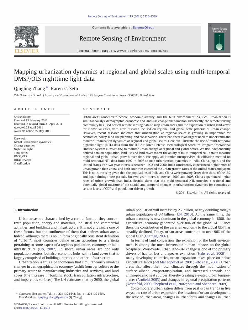
Due to differences in satellite orbits (dawn pass versus dusk pass)and sensor degradation, NTL data collected by sensors onboarddifferent satellites could be significantly different, even when thereare no real changes occurred on the ground. Version 4 includes datafrom five satellites: F10, F12, F14, F15, and F16 (Fig. 1). In theory, atime series of NTL data could capture the dynamics of urbanizationdespite possible errors from sensor differences. This would require thesignal of change to be larger than the error signal and also largeenough to render the error signal (noise) unimportant.

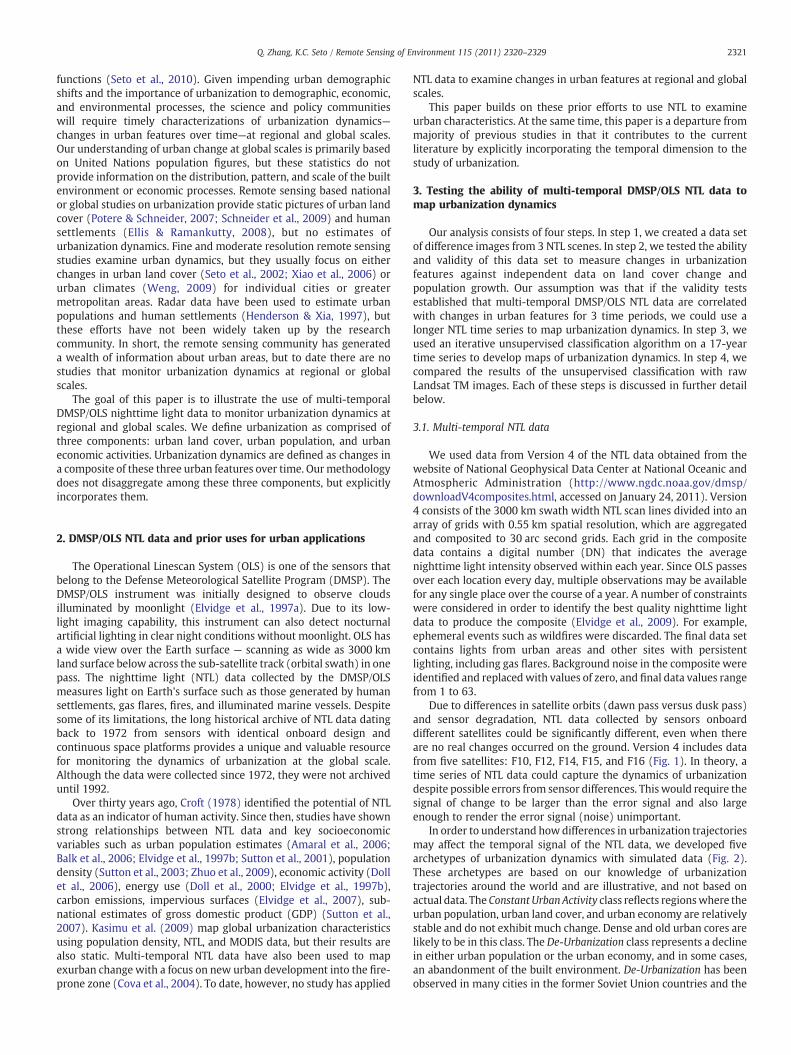
In order to understand how differences in urbanization trajectoriesmay affect the temporal signal of the NTL data, we developed fivearchetypes of urbanization dynamics with simulated data (Fig. 2).These archetypes are based on our knowledge of urbanizationtrajectories around the world and are illustrative, and not based onactual data. The Constant UrbanActivity class reflects regionswhere theurban population, urban land cover, and urban economy are relativelystable and do not exhibit much change. Dense and old urban cores arelikely to be in this class. The De-Urbanization class represents a declinein either urban population or the urban economy, and in some cases,an abandonment of the built environment. De-Urbanization has beenobserved in many cities in the former Soviet Union countries and the

0

10

20

30

40

50

60

70

80

90

5

10

15

20

25

30

1992 1994 1996 1998 2000 2002 2004 2006 2008

Sum

of N

TL

DN

for

US

A (

Mill

ions

)

Sum

of N

TL

DN

(M

illio

ns)

Year

USA

CHINA

INDIA

JAPAN

F10 F12

F14

F15

F16

Fig. 1. NTL time series composed of data from several satellites (F10, F12, F14, F15 andF16). Dotted lines indicate satellite shifting.

2322 Q. Zhang, K.C. Seto / Remote Sensing of Environment 115 (2011) 2320–2329

rust belt in theUS. Areas that experiencedhigher levels of urbanizationin earlier periods are in the Early Urban Growth class, and we expecttheir temporal NTL signature to exhibit a convex temporal shape. Intheory, areas that are closer in proximity to existing urban centers aremore likely to exhibit this pattern. It is important to recall we defineurban as comprised of three components: urban land cover, urbanpopulation, and urban economic activities. Therefore, in this analysis,urban growth refers to any combination of these three components.

In contrast, the Recent Urban Growth class has a concave shape. Theconvex shape of the Early Urban Growth class indicates a fasterdevelopment in earlier years, while the concave shape of the RecentUrban Growth class indicates a faster development in later years.These two classes are “spectrally” broad classes. That is, the variationin temporal signature can be large across space within each of thesetwo classes. Due to the coarse spatial resolution and nature of the NTLdata, an increase in the NTL value does not mean large-scale orwholesale urbanization, such as the conversion of agricultural areas tobuilt-up areas or a large influx of population. In many cases, theincrease in the NTL value is due to an intensification process withinexisting but not densely urbanized areas.

We developed two datasets using the Version 4 NTL data. The firstdataset consists of 17 NTL images, one for each year from 1992 to

0

10

20

30

40

50

60

70

1992 1994 1996 1998 2000 2002 2004 2006 2008

Mea

n N

TL

DN

Year

1. Constant urban activity

2. Early urban growth

3. De-urbanization

4. Constant urban growth

5. Recent urban growth

Fig. 2. Archetypes of different temporal patterns of urbanization dynamics for specificurban areas using simulated data.

2008. The second dataset consists of data for 3 dates, 1992, 2001, and2008, and a simple difference image generated from the 1992 and2008 images: NTL2008−NTL1992. We selected NTL data from those 3dates in order to correspond with the urban population data from theWorld Bank, which are available up to 2008, and land cover data fromthe U.S. National Land Cover Database (NLCD), which spans from 1992to 2001. We used data from these two independent sources to test theability of multi-temporal NTL to monitor urbanization dynamics.

We built linear regression models based on the NTL differenceimages, urban population, and the percentage of new urban develop-ment inside a 1 km grid between 1992 and 2008. For comparisonpurposes we also built linear regression models based on the rates ofcountry-level urban population change worldwide. The urban popu-lation growth rate is defined as (Upop2008−Upop1992)/Upop1992. Thegrowth rate of NTL for each country is defined similarly.

3.2. Independent data on urban land expansion and urban populationgrowth

What is the ability ofmulti-temporal NTL data to track urbanizationdynamics, or changes in urban features?We used two types of validitytests to see if multi-temporal NTL data could successfully monitorurbanization dynamics. First, we compared NTL-derived urbanizationdynamics with World Bank urban population growth data atthe country level from 1992 and 2008 (http://data.worldbank.org/data-catalog/world-development-indicators, accessed on January 10,2011). We overlaid country boundary map from ESRI (2002) onto theNTL imagery to retrieve NTL stats for each administrative unit, countryor area. Not all of the administrative units in the world have urbanpopulation records for the time period of interest. Therefore, of the 238countries or areas, 197with complete recordswere selected for furtheranalysis.

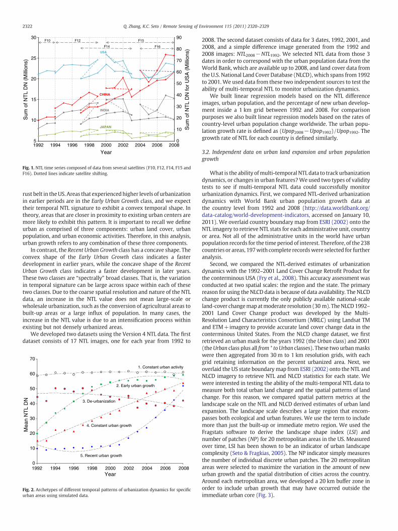
Second, we compared the NTL-derived estimates of urbanizationdynamics with the 1992–2001 Land Cover Change Retrofit Product forthe conterminous USA (Fry et al., 2008). This accuracy assessment wasconducted at two spatial scales: the region and the state. The primaryreason for using the NLCD data is because of data availability. The NLCDchange product is currently the only publicly available national-scaleland-cover changemap atmoderate resolution (30 m). TheNLCD1992–2001 Land Cover Change product was developed by the Multi-Resolution Land Characteristics Consortium (MRLC) using Landsat TMand ETM+imagery to provide accurate land cover change data in theconterminous United States. From the NLCD change dataset, we firstretrieved an urban mask for the years 1992 (the Urban class) and 2001(theUrban class plus all from * to Urban classes). These two urbanmaskswere then aggregated from 30 m to 1 km resolution grids, with eachgrid retaining information on the percent urbanized area. Next, weoverlaid the US state boundarymap from ESRI (2002) onto the NTL andNLCD imagery to retrieve NTL and NLCD statistics for each state. Wewere interested in testing the ability of the multi-temporal NTL data tomeasure both total urban land change and the spatial patterns of landchange. For this reason, we compared spatial pattern metrics at thelandscape scale on the NTL and NLCD derived estimates of urban landexpansion. The landscape scale describes a large region that encom-passes both ecological and urban features. We use the term to includemore than just the built-up or immediate metro region. We used theFragstats software to derive the landscape shape index (LSI) andnumber of patches (NP) for 20 metropolitan areas in the US. Measuredover time, LSI has been shown to be an indicator of urban landscapecomplexity (Seto & Fragkias, 2005). The NP indicator simply measuresthe number of individual discrete urban patches. The 20 metropolitanareas were selected to maximize the variation in the amount of newurban growth and the spatial distribution of cities across the country.Around each metropolitan area, we developed a 20 km buffer zone inorder to include urban growth that may have occurred outside theimmediate urban core (Fig. 3).

NLCD New Urban

Metro Areas

States0 450 900 1,350225

Km

Fig. 3. The 20 metropolitan areas in the conterminous US selected for calculating landscape metrics for testing the validity tests. The red areas are new urban development retrievedfrom the NLCD change product during the 1992–2001 period.

2323Q. Zhang, K.C. Seto / Remote Sensing of Environment 115 (2011) 2320–2329

4. Results of validity tests

4.1. Validity tests using country-level population data

The country boundaries do not cover oceans and therefore fishinglights on open waters were discarded from calculating NTL statistics.NTL differences between 1992 and 2008 were calculated for eachcountry or area as follows: Sum2008−Sum1992. Urban population(Upop) differences were retrieved in the same way: Upop2008−Upop1992. To minimize the scale differences between the NTL andurban population data, we applied a classic data normalizationscheme:

xi−x′z

ð1Þ

China

India

IndonesiaUnited States

Brazil

NigeriaPhilippines

Sudan

Australia

Greenland

Russia

y = 0.6709x - 2E-17R² = 0.45

-10

-8

-6

-4

-2

0

2

4

6

8

10

-2 0 2 4 6 8 10 12

Nor

mal

ized

NT

L di

ffere

nce

by c

ount

ry b

etw

een

1992

and

200

8

Normalized urban population difference by country between 19and 2008

a

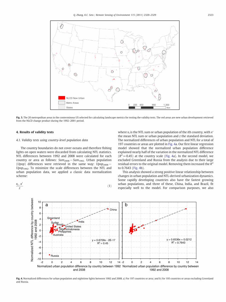
Fig. 4.Normalized differences for urban population and nighttime lights between 1992 and 2and Russia.

where xi is the NTL sum or urban population of the ith country, with x′the mean NTL sum or urban population and z the standard deviation.The normalized differences of urban population and NTL for a total of197 countries or areas are plotted in Fig. 4a. Our first linear regressionmodel showed that the normalized urban population differenceexplained nearly half of the variation in the normalized NTL difference(R2=0.45) at the country scale (Fig. 4a). In the second model, weexcluded Greenland and Russia from the analysis due to their largeresidual errors to the original model. Removing them increased the R2

to 0.7643 (Fig. 4b).This analysis showed a strong positive linear relationship between

changes in urban population and NTL-derived urbanization dynamics.Some rapidly developing countries also have the fastest growingurban populations, and three of these, China, India, and Brazil, fitespecially well to the model. For comparison purposes, we also

y = 0.6536x + 0.0212R² = 0.7643

-2 0 2 4 6 8 10 12 14

Normalized urban population difference by country between1992 and 2008

b

14

92

008. a) For 197 countries or area; and b) for 195 countries or areas excluding Greenland

y = 1.0836x + 0.0659R² = 0.2204

-1

-0.5

0

0.5

1

-0.5 -0.3 -0.1 0.1 0.3

Normalized urban population difference by countrybetween 1992 and 2008

by = 0.1893x + 0.3883R² = 0.0481

-0.5

0

0.5

1

1.5

2

-0.5 0 0.5 1 1.5 2 2.5

Nor

mal

ized

NT

L gr

owth

rat

e by

cou

ntry

betw

een

1992

and

200

8

Normalized urban population growth rate by countrybetween 1992 and 2008

a

Fig. 5. a) Normalized growth rates for urban population and nighttime lights between 1992 and 2008 for 197 countries; and b) Normalized differences of urban population andnighttime light for countries that experienced slow urban growth between 1992 and 2008.

Texas

Florida

y = 0.0062x - 68.772R² = 0.5737

-1

0

1

2

3

4

5

6

7

8

9

10

0 2 4 6 8 10 12

x100

0

x100000

Fig. 6. Urban land expansion in the 49 conterminous US states between 1992 and 2001,as detected by NLCD and NTL.

2324 Q. Zhang, K.C. Seto / Remote Sensing of Environment 115 (2011) 2320–2329

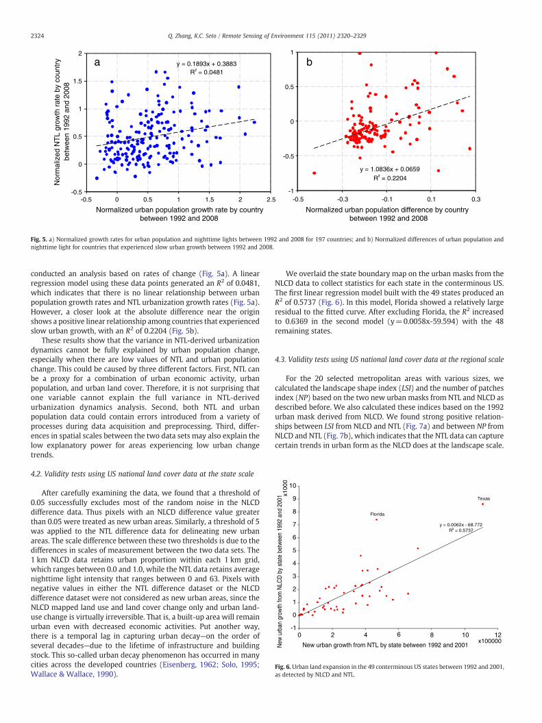
conducted an analysis based on rates of change (Fig. 5a). A linearregression model using these data points generated an R2 of 0.0481,which indicates that there is no linear relationship between urbanpopulation growth rates and NTL urbanization growth rates (Fig. 5a).However, a closer look at the absolute difference near the originshows a positive linear relationship among countries that experiencedslow urban growth, with an R2 of 0.2204 (Fig. 5b).

These results show that the variance in NTL-derived urbanizationdynamics cannot be fully explained by urban population change,especially when there are low values of NTL and urban populationchange. This could be caused by three different factors. First, NTL canbe a proxy for a combination of urban economic activity, urbanpopulation, and urban land cover. Therefore, it is not surprising thatone variable cannot explain the full variance in NTL-derivedurbanization dynamics analysis. Second, both NTL and urbanpopulation data could contain errors introduced from a variety ofprocesses during data acquisition and preprocessing. Third, differ-ences in spatial scales between the two data sets may also explain thelow explanatory power for areas experiencing low urban changetrends.

4.2. Validity tests using US national land cover data at the state scale

After carefully examining the data, we found that a threshold of0.05 successfully excludes most of the random noise in the NLCDdifference data. Thus pixels with an NLCD difference value greaterthan 0.05 were treated as new urban areas. Similarly, a threshold of 5was applied to the NTL difference data for delineating new urbanareas. The scale difference between these two thresholds is due to thedifferences in scales of measurement between the two data sets. The1 km NLCD data retains urban proportion within each 1 km grid,which ranges between 0.0 and 1.0, while the NTL data retains averagenighttime light intensity that ranges between 0 and 63. Pixels withnegative values in either the NTL difference dataset or the NLCDdifference dataset were not considered as new urban areas, since theNLCD mapped land use and land cover change only and urban land-use change is virtually irreversible. That is, a built-up area will remainurban even with decreased economic activities. Put another way,there is a temporal lag in capturing urban decay—on the order ofseveral decades—due to the lifetime of infrastructure and buildingstock. This so-called urban decay phenomenon has occurred in manycities across the developed countries (Eisenberg, 1962; Solo, 1995;Wallace & Wallace, 1990).

We overlaid the state boundary map on the urban masks from theNLCD data to collect statistics for each state in the conterminous US.The first linear regression model built with the 49 states produced anR2 of 0.5737 (Fig. 6). In this model, Florida showed a relatively largeresidual to the fitted curve. After excluding Florida, the R2 increasedto 0.6369 in the second model (y=0.0058x-59.594) with the 48remaining states.

4.3. Validity tests using US national land cover data at the regional scale

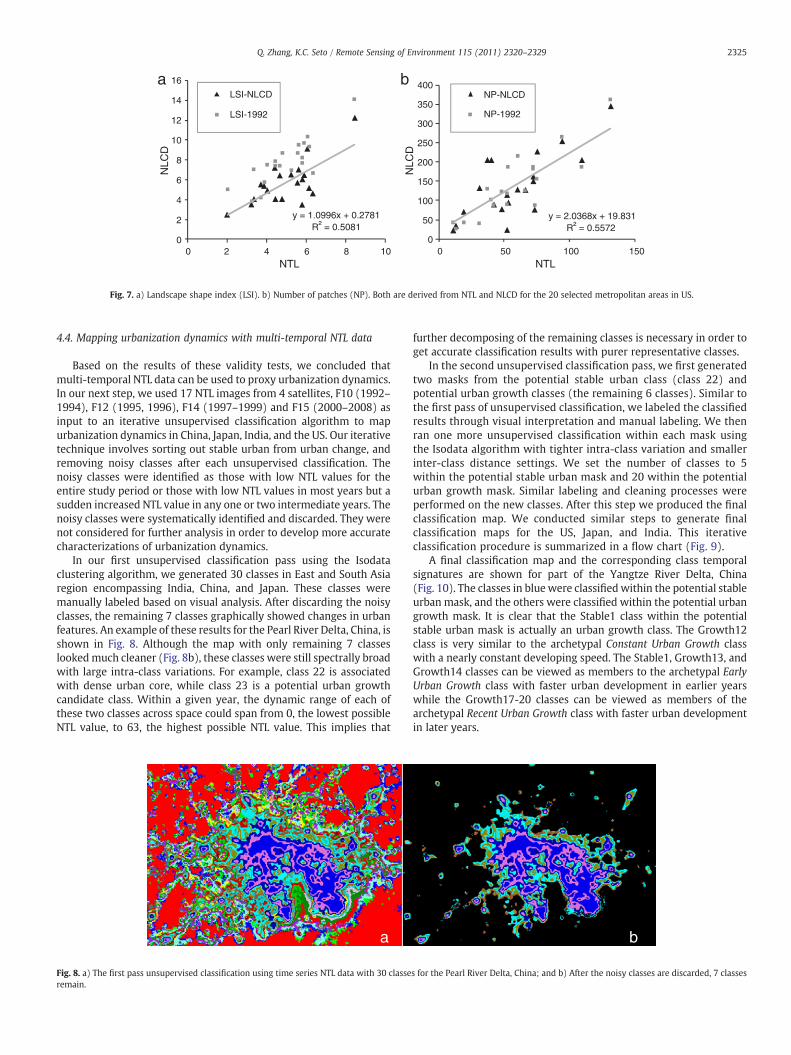
For the 20 selected metropolitan areas with various sizes, wecalculated the landscape shape index (LSI) and the number of patchesindex (NP) based on the two new urban masks from NTL and NLCD asdescribed before. We also calculated these indices based on the 1992urban mask derived from NLCD. We found strong positive relation-ships between LSI from NLCD and NTL (Fig. 7a) and between NP fromNLCD and NTL (Fig. 7b), which indicates that the NTL data can capturecertain trends in urban form as the NLCD does at the landscape scale.

y = 1.0996x + 0.2781R² = 0.5081

0

2

4

6

8

10

12

14

16

0 2 4 6 8 10

NLC

D

NTL NTL

LSI-NLCD

LSI-1992

a

y = 2.0368x + 19.831R² = 0.5572

0

50

100

150

200

250

300

350

400

0 50 100 150

NLC

D

NP-NLCD

NP-1992

b

Fig. 7. a) Landscape shape index (LSI). b) Number of patches (NP). Both are derived from NTL and NLCD for the 20 selected metropolitan areas in US.

2325Q. Zhang, K.C. Seto / Remote Sensing of Environment 115 (2011) 2320–2329

4.4. Mapping urbanization dynamics with multi-temporal NTL data

Based on the results of these validity tests, we concluded thatmulti-temporal NTL data can be used to proxy urbanization dynamics.In our next step, we used 17 NTL images from 4 satellites, F10 (1992–1994), F12 (1995, 1996), F14 (1997–1999) and F15 (2000–2008) asinput to an iterative unsupervised classification algorithm to mapurbanization dynamics in China, Japan, India, and the US. Our iterativetechnique involves sorting out stable urban from urban change, andremoving noisy classes after each unsupervised classification. Thenoisy classes were identified as those with low NTL values for theentire study period or those with low NTL values in most years but asudden increased NTL value in any one or two intermediate years. Thenoisy classes were systematically identified and discarded. They werenot considered for further analysis in order to develop more accuratecharacterizations of urbanization dynamics.

In our first unsupervised classification pass using the Isodataclustering algorithm, we generated 30 classes in East and South Asiaregion encompassing India, China, and Japan. These classes weremanually labeled based on visual analysis. After discarding the noisyclasses, the remaining 7 classes graphically showed changes in urbanfeatures. An example of these results for the Pearl River Delta, China, isshown in Fig. 8. Although the map with only remaining 7 classeslookedmuch cleaner (Fig. 8b), these classes were still spectrally broadwith large intra-class variations. For example, class 22 is associatedwith dense urban core, while class 23 is a potential urban growthcandidate class. Within a given year, the dynamic range of each ofthese two classes across space could span from 0, the lowest possibleNTL value, to 63, the highest possible NTL value. This implies that

a

Fig. 8. a) The first pass unsupervised classification using time series NTL data with 30 classeremain.

further decomposing of the remaining classes is necessary in order toget accurate classification results with purer representative classes.

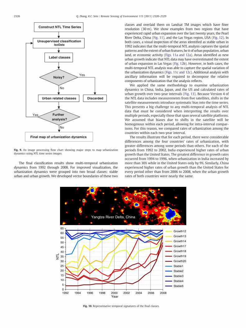
In the second unsupervised classification pass, we first generatedtwo masks from the potential stable urban class (class 22) andpotential urban growth classes (the remaining 6 classes). Similar tothe first pass of unsupervised classification, we labeled the classifiedresults through visual interpretation and manual labeling. We thenran one more unsupervised classification within each mask usingthe Isodata algorithm with tighter intra-class variation and smallerinter-class distance settings. We set the number of classes to 5within the potential stable urban mask and 20 within the potentialurban growth mask. Similar labeling and cleaning processes wereperformed on the new classes. After this step we produced the finalclassification map. We conducted similar steps to generate finalclassification maps for the US, Japan, and India. This iterativeclassification procedure is summarized in a flow chart (Fig. 9).

A final classification map and the corresponding class temporalsignatures are shown for part of the Yangtze River Delta, China(Fig. 10). The classes in blue were classifiedwithin the potential stableurban mask, and the others were classified within the potential urbangrowth mask. It is clear that the Stable1 class within the potentialstable urban mask is actually an urban growth class. The Growth12class is very similar to the archetypal Constant Urban Growth classwith a nearly constant developing speed. The Stable1, Growth13, andGrowth14 classes can be viewed as members to the archetypal EarlyUrban Growth class with faster urban development in earlier yearswhile the Growth17-20 classes can be viewed as members of thearchetypal Recent Urban Growth class with faster urban developmentin later years.

b

s for the Pearl River Delta, China; and b) After the noisy classes are discarded, 7 classes

Construct NTL Time Series

Unsupervised classificationIsoData

Discarded

Label classes

Urban related classes

Final map of urbanization dynamics

Noisy?

Furtheranalysis?

No

Yes

Yes

No

Fig. 9. An image processing flow chart showing major steps to map urbanizationdynamics using NTL time series images.

2326 Q. Zhang, K.C. Seto / Remote Sensing of Environment 115 (2011) 2320–2329

The final classification results show multi-temporal urbanizationdynamics from 1992 through 2008. For improved visualization, theurbanization dynamics were grouped into two broad classes: stableurban and urban growth. We developed vector boundaries of these two

0

5

10

15

20

25

30

35

40

45

50

55

60

65

1992 1994 1996 1998 2000 2

NT

L

Year

Yangtze River Delta

Fig. 10. Representative temporal s

classes and overlaid them on Landsat TM images which have finerresolution (30 m). We show examples from two regions that haveexperienced rapid urban expansion over the last twenty years, the PearlRiver Delta, China (Fig. 11), and the Las Vegas region, USA (Fig. 12). Inboth cases, a visual inspection of the areas identified as stable urban in1992 indicates that the multi-temporal NTL analysis captures the spatialpatterns and theextent of urban features, be it of urbanpopulation, urbanland, or economic activity (Figs. 11a and 12a). Areas identified as newurban growth indicate that NTL datamay have overestimated the extentof urban expansion in Las Vegas (Fig. 12b). However, in both cases, themulti-temporal NTL analysis was able to capture the spatial variation ofthe urbanization dynamics (Figs. 11c and 12c). Additional analysis withancillary information will be required to decompose the relativecomponents of urbanization that the analysis reflects.

We applied the same methodology to examine urbanizationdynamics in China, India, Japan, and the US and calculated rates ofurban growth over two-year intervals (Fig. 13). Because Version 4 ofthe NTL data includes measurements from five satellites, shifts in thesatellite measurements introduce systematic bias into the time series.This presents a big challenge to any multi-temporal analysis of NTLdata that must be considered when interpreting the results overmultiple periods, especially those that span several satellite platforms.We assumed that biases due to shifts in the satellite will behomogenous within each period, allowing for intra-interval compar-isons. For this reason, we compared rates of urbanization among thecountries within each two-year interval.

The results illustrate that for each period, there were considerabledifferences among the four countries' rates of urbanization, withgreater differences among some periods than others. For each of theperiods from 1992 to 2002, India experienced higher rates of urbangrowth than the United States. The greatest difference in growth ratesoccurred from 1994 to 1996, when urbanization in India increased bymore than 30% while in the United States only by 9%. Similarly, Chinaexperienced higher rates of urban growth than the United States forevery period other than from 2006 to 2008, when the urban growthrates of both countries were nearly the same.

002 2004 2006 2008

Growth12

Growth13

Growth14

Growth17

Growth18

Growth19

Growth20

Stable1

Stable2

Stable3

Stable4

Stable5

, China

ignatures of the final classes.

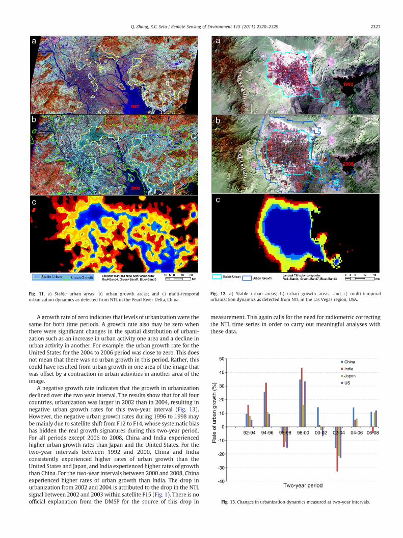
Fig. 11. a) Stable urban areas; b) urban growth areas; and c) multi-temporalurbanization dynamics as detected from NTL in the Pearl River Delta, China.

Fig. 12. a) Stable urban areas; b) urban growth areas; and c) multi-temporalurbanization dynamics as detected from NTL in the Las Vegas region, USA.

-40

-30

-20

-10

0

10

20

30

40

50

92-94 94-96 96-98 98-00 00-02 02-04 04-06 06-08

Rat

e of

urb

an g

row

th (

%)

Two-year period

China

India

Japan

US

Fig. 13. Changes in urbanization dynamics measured at two-year intervals.

2327Q. Zhang, K.C. Seto / Remote Sensing of Environment 115 (2011) 2320–2329

A growth rate of zero indicates that levels of urbanization were thesame for both time periods. A growth rate also may be zero whenthere were significant changes in the spatial distribution of urbani-zation such as an increase in urban activity one area and a decline inurban activity in another. For example, the urban growth rate for theUnited States for the 2004 to 2006 period was close to zero. This doesnot mean that there was no urban growth in this period. Rather, thiscould have resulted from urban growth in one area of the image thatwas offset by a contraction in urban activities in another area of theimage.

A negative growth rate indicates that the growth in urbanizationdeclined over the two year interval. The results show that for all fourcountries, urbanization was larger in 2002 than in 2004, resulting innegative urban growth rates for this two-year interval (Fig. 13).However, the negative urban growth rates during 1996 to 1998 maybe mainly due to satellite shift from F12 to F14, whose systematic biashas hidden the real growth signatures during this two-year period.For all periods except 2006 to 2008, China and India experiencedhigher urban growth rates than Japan and the United States. For thetwo-year intervals between 1992 and 2000, China and Indiaconsistently experienced higher rates of urban growth than theUnited States and Japan, and India experienced higher rates of growththan China. For the two-year intervals between 2000 and 2008, Chinaexperienced higher rates of urban growth than India. The drop inurbanization from 2002 and 2004 is attributed to the drop in the NTLsignal between 2002 and 2003 within satellite F15 (Fig. 1). There is noofficial explanation from the DMSP for the source of this drop in

measurement. This again calls for the need for radiometric correctingthe NTL time series in order to carry out meaningful analyses withthese data.

2328 Q. Zhang, K.C. Seto / Remote Sensing of Environment 115 (2011) 2320–2329

5. Discussion

Given the magnitude of the global urban transition of the 21stcentury, there is an urgent need for accurate and timely informationon how urban areas are changing across multiple dimensions.Urbanization as a demographic, economic, and land change processhas not been mapped spatially at the global scale very well. Withestimates that the global urban population will increase by another3 billion by 2030, the number and size of urban areas will need togrow significantly to house the world's growing urban population.And yet, we have very little understanding of the spatial configurationof the first 3 billion urban inhabitants, changes in the urban economy,and how urbanization has shaped urban land cover dynamicsworldwide. This study contributes to addressing these issues.

The results from the multi-temporal NTL analysis show a fewtrends in the spatial and temporal dynamics of urbanization. First,there exist different temporal trajectories of urbanization and theseare distinguishable with multi-temporal NTL data, as illustrated bytheir temporal signatures (Fig. 10). Across many disciplines in boththe social and natural sciences, there is a growing interest inunderstanding how urbanization is driven by policy and socioeco-nomic changes and how these urban changes in turn are drivingglobal environmental change. For example, economic studies showthat manufacturing, financial, and industrial activities aggregate inspace (Brülhart & Sbergami, 2009; Duranton & Puga, 2004), but thelinks between policy and spatial form of urban areas or their growthhave not been well documented. The results here show that it ispossible to identify spatial and temporal trajectories of urbanizationdynamics and development of these data sets may facilitate the studyof the links between policy and urban change.

Second, the results show large variations in temporal patterns ofurbanization dynamics, which in turn underscore the importance ofexamining changes in urban features over time and across hightemporal frequencies. There is no definition of high temporalfrequency in the literature, but we argue that temporal frequency isrelative to the total time span of the study and the study location. Forexample, a study spanning twenty years with one satellite image fromevery four years would generate a time series of five images.Conversely, a study spanning one year using five intra-year imagescould be considered high temporal frequency. Just as spatialresolution refers to both grain size and study extent, temporalresolution refers to both the total span of a study (i.e., number of yearsbetween start and end date) and the frequency of observations withinthe study (i.e., number of satellite observations between the start andend date). Higher temporal frequency observations may introducemore noise, but is necessary to capture the trends in the many rapidlyurbanizing places around theworld. Additionally, we can only identifylarge variations in urbanization dynamics across regions with the useof high temporal frequency data spanning long time periods. The two-year intervals of urbanization rates highlight these variations.Currently, a majority of studies on urban change use data fromseveral points in time over long time spans but few studiesincorporate high temporal frequencies of observations. Urbanchanges are punctuated by temporal patterns that reflect changes indemographic patterns, policy shifts, and economic development, butthese changes have only been quantified at the city scale (Seto &Fragkias, 2005).

Third, the results show large variations in the spatial patterns ofurbanization over time. The results from the Pearl River Delta and LasVegas illustrate these differences. Whereas Las Vegas grew in a classicvon Thünen fashion (Thünen, 1875), the urbanization dynamics of thePearl River Delta were more piecemeal in nature. These differencesreflect differences in scale and policy. Las Vegas is a single citywhereas the Pearl River Delta is a region comprised of more than adozen cities. What do these multi-temporal maps of urbanizationdynamics reveal? In the case of Las Vegas, the results indicate that

urban growth – be it the increase in the urban population, theexpansion of urban land cover, or the development of the urbaneconomy – largely occurred close to existing urban areas. At thespatial scale of the NTL data, there were no large leapfrogging patternsof urban expansion. In contrast, the spatial configuration of urbanchange in the Pearl River Delta is patchy. Much of the urban expansionis discontinuous from existing urban areas and leapfrog developmentis prevalent.

Despite the ability of multi-temporal NTL data to delineateurbanization dynamics, challenges remain. First, accuracy assessingthe maps of urbanization dynamics will be difficult. Our researchgroup has been studying the Pearl River Delta for over fifteen years,and we have generated some of the longest datasets of the regionusing Landsat TM. With an archive of 22 classified images spanningeach year from 1988 to 2009, we were able to use these data to assessthe quality of the multi-temporal NTL results. This type of accuracyassessment with higher resolution data for multiple time points isdifficult to carry out over one study site, much less at regional orglobal scales.

Second, oversaturation of NTL data can blur the temporal andspatial signatures of urban change. It is important to point out that weignored the oversaturation effects when we calculated the NTLstatistics. During the NTL data acquisition, any area with lightintensity above a certain level (usually a dense urban core) will beassigned a DN of 63, themaximum value in the final NTL products. Weassumed that there would be low or no change in the NTL brightnessonce an area's brightness reaches certain level. This assumption maybe true in most areas, but can be problematic. Some studies haveproposed methods to bring meaningful estimates to correct the lightsaturation effects. For example, Letu et al. (2010) applied a cubicregression equation to correct the saturated light and estimatedelectric power consumption with high precision from the correctedstable light. However, oversaturation can still remain an issue.

Third, there are significant differences in the radiometric signa-tures across the different DMSP/OLS satellites. In our exploratory dataanalysis, we found it difficult to compare across satellites due todifferences in mean NTL values. Even in the same year when there areNTL observations from two different satellites available, there may besystematic significant deviation one from another.We discarded somedata that look systematically biased when compared with other datain the time series, in order to minimize errors arising from satellitedifference. More accurate calibration of the NTL data, especiallybetween satellites that take measurement in the same period, will behelpful to solve this issue.

6. Conclusions

As we embark on the second decade of the “Century of the City”,there is a growing demand for information on changes in urbanizationcharacteristics over multiple time periods and for large geographicareas. Thus far, the remote sensing community has made significantcontributions inmapping urban change at local scales. However, thesetypes of multi-temporal assessments of urban change have notoccurred at regional or global scales.

Multi-temporal nighttime lights data have enormous potential toshed light on urbanization processes at regional and global scales. Thehigh correlation between NTL and some social economic variablessuch as urban population and GDP indicates that NTL can be used as aproxy for these variables at the country and regional scales, especiallywhen the social and economic data are not available. In this study, weexamine the utility of multi-temporal NTL data to measure urbani-zation dynamics. The method we propose in this study is a firstattempt at using multi-temporal NTL data to evaluate changes inurban features over time. Althoughmost of the examples in this paperwere at the regional scale, the method could be easily and quicklyapplied at global scales. Our hope is that by illustrating the utility of

2329Q. Zhang, K.C. Seto / Remote Sensing of Environment 115 (2011) 2320–2329

multi-temporal NTL data for mapping urbanization dynamics, weencourage additional studies that evaluate the changes in urbanfeatures over time and at scales beyond the individual city.

Acknowledgments

This study was supported by NASA grant NNX11AE88G. We thankBurak Güneralp, Michail Fragkias and Peter Christensen for theirdiscussions and feedback during earlier phases of this research. Wethank the two anonymous reviewers whose suggestions helped toimprove the clarity of the manuscript.

References

Amaral, S., Monteiro, A., Camara, G., & Quintanilha, J. (2006). DMSP/OLS night-time lightimagery for urban population estimates in the Brazilian Amazon. InternationalJournal of Remote Sensing, 27, 855–870.

Arnfield, A. (2003). Two decades of urban climate research: a review of turbulence,exchanges of energy and water, and the urban heat island. International Journal ofClimatology, 23, 1–26.

Balk, D., Deichmann, U., Yetman, G., Pozzi, F., Hay, S., & Nelson, A. (2006). Determiningglobal population distribution: Methods, applications and data. Advances inParasitology, 62, 119–156.

Brülhart, M., & Sbergami, F. (2009). Agglomeration and growth: Cross-countryevidence. Journal of Urban Economics, 65, 48–63.

Cova, T., Sutton, P., & Theobald, D. (2004). Exurban change detection in fire-prone areaswith nighttime satellite imagery. Photogrammetric Engineering and Remote Sensing,70, 1249–1258.

Croft, T. (1978). Nighttime images of the earth from space. Scientific American, 239,86–98.

del Mar López, T., Aide, T., & Thomlinson, J. (2001). Urban expansion and the loss ofprime agricultural lands in Puerto Rico. Ambio, 30, 49–54.

Doll, C., Muller, J., & Elvidge, C. (2000). Night-time imagery as a tool for global mappingof socioeconomic parameters and greenhouse gas emissions. Ambio, 29, 157–162.

Doll, C., Muller, J., & Morley, J. (2006). Mapping regional economic activity from night-time light satellite imagery. Ecological Economics, 57, 75–92.

Duranton, G., & Puga, D. (2004). Micro-foundations of urban agglomeration economies.Handbook of Regional and Urban Economics, 4, 2063–2117.

Eisenberg, L. (1962). The sins of the fathers: Urban decay and social pathology. TheAmerican Journal of Orthopsychiatry, 32, 5–17.

Ellis, E., & Ramankutty, N. (2008). Putting people in the map: Anthropogenic biomes ofthe world. Frontiers in Ecology and the Environment, 6, 439–447.

Elvidge, C., Baugh, K., Kihn, E., Kroehl, H., & Davis, E. (1997a). Mapping city lights withnighttime data from the DMSP Operational Linescan System. PhotogrammetricEngineering and Remote Sensing, 63, 727–734.

Elvidge, C., Baugh, K., Kihn, E., Kroehl, H., Davis, E., & Davis, C. (1997b). Relation betweensatellite observed visible-near infrared emissions, population, economic activity andelectric power consumption. International Journal of Remote Sensing, 18, 1373–1379.

Elvidge, C., Erwin, E., Baugh, K., Ziskin, D., Tuttle, B., Ghosh, T., et al. (2009). Overview ofDMSP nightime lights and future possibilities. IEEE Proceedings of the 7thInternational Urban Remote Sensing Conference.

Elvidge, C., Tuttle, B., Sutton, P., Baugh, K., Howard, A., Milesi, C., et al. (2007). Globaldistribution and density of constructed impervious surfaces. Sensors, 7, 1962–1979.

ESRI (2002). ESRI Data & Maps [CD-ROM]. Redlands, CA: Environmental SystemsResearch Institute.

Fry, J., Coan, M., Homer, C., Meyer, D., &Wickham, J. (2008). Completion of the NationalLand Cover Database (NLCD) 1992–2001 Land Cover Change Retrofit Product. USGeological Survey Open-File Report, 1379, 18.

Gutman, P. (2007). Ecosystem services: Foundations for a new rural-urban compact.Ecological Economics, 62, 383–387.

Hahs, A., McDonnell, M., McCarthy, M., Vesk, P., Corlett, R., Norton, B., et al. (2009). Aglobal synthesis of plant extinction rates in urban areas. Ecology Letters, 12,1165–1173.

Henderson, F., & Xia, Z. (1997). SAR applications in human settlement detection,populationestimation and urban land use pattern analysis: A status report. IEEETransactions on Geoscience and Remote Sensing, 35, 79–85.

Kasimu, A., Tateishi, R., & Hoan, N. (2009). Global urban characterization usingpopulation density, DMSP and MODIS data. 2009 Urban Remote Sensing Joint Event(pp. 1–7). IEEE.

Letu, H., Hara, M., Yagi, H., Naoki, K., Tana, G., Nishio, F., et al. (2010). Estimating energyconsumption from night-time DMPS/OLS imagery after correcting for saturationeffects. International Journal of Remote Sensing, 31, 4443–4458.

Potere, D., & Schneider, A. (2007). A critical look at representations of urban areas inglobal maps. GeoJournal, 69, 55–80.

Rosenfeld, D. (2000). Suppression of rain and snow by urban and industrial airpollution. Science, 287, 1793.

Schneider, A., Friedl, M. A., & Potere, D. (2009). A new map of global urban extent fromMODIS satellite data. Environmental Research Letters, 044003.

Seto, K., & Fragkias, M. (2005). Quantifying spatiotemporal patterns of urban land-usechange in four cities of China with time series landscapemetrics. Landscape Ecology,20, 871–888.

Seto, K., Kaufmann, R., & Woodcock, C. (2000). Landsat reveals China's farmlandreserves, but they're vanishing fast. Nature, 406, 121.

Seto, K., Sánchez-Rodríguez, R., & Fragkias, M. (2010). The new geography ofcontemporary urbanization and the environment. Annual review of environmentand resources.

Seto, K., & Shepherd, M. (2009). Global urban land-use trends and climate impacts.Current Opinion in Environmental Sustainability, 1, 89–95.

Seto, K., Woodcock, C., Song, C., Huang, X., Lu, J., & Kaufmann, R. (2002). Monitoringland-use change in the Pearl River Delta using Landsat TM. International Journal ofRemote Sensing, 23, 1985–2004.

Shepherd, J., Pierce, H., & Negri, A. (2002). Rainfall modification by major urban areas:Observations from spaceborne rain radar on the TRMM satellite. Journal of AppliedMeteorology, 41, 689–701.

Solo, J. (1995). Urban decay and the role of superfund: Legal barriers to redevelopmentand prospects for change. Buffalo Law Review, 43, 285.

Sutton, P., Elvidge, C., & Ghosh, T. (2007). Estimation of gross domestic product at sub-national scales using nighttime satellite imagery. International Journal of EcologicalEconomics & Statistics, 8, 5–21.

Sutton, P., Elvidge, C., & Obremski, T. (2003). Building and evaluating models toestimate ambient population density. Photogrammetric Engineering and RemoteSensing, 69, 545–554.

Sutton, P., Roberts, D., Elvidge, C., & Baugh, K. (2001). Census from Heaven: An estimateof the global human population using night-time satellite imagery. InternationalJournal of Remote Sensing, 22, 3061–3076.

Thünen, V. (1875). Der isolierte Staat. Berlin: Wiegandt, Hempel & Parey.UN (2007). Table 6. Definition of “Urban”. Demographic Yearbook 2005. New york:

United Nations.UN (2010). World urbanization prospects, 2009 revision. New York: United Nations.Wallace, R., &Wallace, D. (1990). Origins of public health collapse in New York City: The

dynamics of planned shrinkage, contagious urban decay and social disintegration.Bulletin of the New York Academy of Medicine, 66, 391.

Weng, Q. (2009). Thermal infrared remote sensing for urban climate and environ-mental studies: Methods, applications, and trends. ISPRS Journal of Photogrammetryand Remote Sensing, 64, 335–344.

Xiao, J., Shen, Y., Ge, J., Tateishi, R., Tang, C., Liang, Y., et al. (2006). Evaluating urbanexpansion and land use change in Shijiazhuang, China, by using GIS and remotesensing. Landscape and Urban Planning, 75, 69–80.

Zhuo, L., Ichinose, T., Zheng, J., Chen, J., Shi, P., & Li, X. (2009). Modelling the populationdensity of China at the pixel level based on DMSP/OLS non-radiance-calibratednight-time light images. International Journal of Remote Sensing, 30, 1003–1018.