remote sensing and gis applications meteorology
TRANSCRIPT
Satellite Remote Sensing andGIS Applications in
Agricultural Meteorology
Proceedings of the Training Workshop7-11 July, 2003, Dehra Dun, India
EditorsM.V.K. Sivakumar
P.S. RoyK. Harmsen
S.K. Saha
SponsorsWorld Meteorological Organization (WMO)
India Meteorological Department (IMD)Centre for Space Science and Technology Education in Asia and the Pacific
(CSSTEAP)Indian Institute of Remote Sensing (IIRS)
National Remote Sensing Agency (NRSA) andSpace Application Centre (SAC)
AGM-8WMO/TD No. 1182
World Meteorological Organisation7bis, Avenue de la Paix
1211 Geneva 2Switzerland
2004

Published byWorld Meteorological Organisation7bis, Avenue de la Paix1211 Geneva 2, Switzerland
© World Meteorological Organisation
All rights reserved. No part of this publication may be reproduced, stored in a retrieval system,or transmitted in any form or by any means, electronic, mechanical, photocopying, recording,or otherwise, without the prior written consent of the copyright owner.
Typesetting and Printing :M/s Bishen Singh Mahendra Pal Singh23-A New Connaught Place, P.O. Box 137,Dehra Dun -248001 (Uttaranchal), INDIAPh.: 91-135-2715748 Fax- 91-135-2715107E.mail: [email protected]: http://www.bishensinghbooks.com
FOREWORD
CONTENTS
Satellite Remote Sensing and GIS Applications in Agricultural .... 1Meteorology and WMO Satellite Activities– M.V.K. Sivakumar and Donald E. Hinsman
Principles of Remote Sensing ......... 23� Shefali Aggarwal
Earth Resource Satellites ......... 39– Shefali Aggarwal
Meteorological Satellites ......... 67– C.M. Kishtawal
Digital Image Processing ......... 81– Minakshi Kumar
Fundamentals of Geographical Information System ......... 103– P.L.N. Raju
Fundamentals of GPS ......... 121– P.L.N. Raju
Spatial Data Analysis ......... 151– P.L.N. Raju
Retrieval of Agrometeorological Parameters using Satellite ......... 175Remote Sensing data– S. K. Saha
Retrieval of Agrometeorological Parameters from Satellites ......... 195 – C.M. Kishtawal
Remote Sensing and GIS Application in Agro-ecological ......... 213zoning– N.R. Patel
Crop Growth Modeling and its Applications in ......... 235Agricultural Meteorology– V. Radha Krishna Murthy

Crop Growth and Productivity Monitoring and Simulation ......... 263using Remote Sensing and GIS– V.K. Dadhwal
Droughts & Floods Assessment and Monitoring using ......... 291Remote Sensing and GIS– A.T. Jeyaseelan
Water and Wind induced Soil Erosion Assessment and ......... 315Monitoring using Remote Sensing and GIS– S.K. Saha
Satellite-based Weather Forecasting ......... 331– S.R. Kalsi
Satellite-based Agro-advisory Service ......... 347– H. P. Das
Forest Fire and Degradation Assessment using Satellite Remote ........ 361Sensing and Geographic Information System– P.S. Roy
Desert Locust Monitoring System–Remote Sensing and GIS ......... 401based approach– D. Dutta, S. Bhatawdekar, B. Chandrasekharan, J.R. Sharma, S. Adiga, Duncan Wood and Adrian McCardle
Workshop Evaluation ......... 425– M.V.K. Sivakumar
SATELLITE REMOTE SENSING AND GISAPPLICATIONS IN AGRICULTURAL METEO-ROLOGY AND WMO SATELLITE ACTIVITIES
M.V.K. Sivakumar and Donald E. HinsmanAgricultural Meteorology Division and Satellite Activities OfficeWorld Meteorological Organization (WMO), 7bis Avenue de la Paix,1211 Geneva 2, Switzerland
Abstract : Agricultural planning and use of agricultural technologies needapplications of agricultural meteorology. Satellite remote sensing technology isincreasingly gaining recognition as an important source of agrometeorological dataas it can complement well the traditional methods agrometeorological datacollection. Agrometeorologists all over the world are now able to take advantageof a wealth of observational data, product and services flowing from speciallyequipped and highly sophisticated environmental observation satellites. In addition,Geographic Information Systems (GIS) technology is becoming an essential toolfor combining various map and satellite information sources in models that simulatethe interactions of complex natural systems. The Commission for AgriculturalMeteorology of WMO has been active in the area of remote sensing and GISapplications in agrometeorology. The paper provides a brief overview of the satelliteremote sensing and GIS Applications in agricultural meteorology along with adescription of the WMO Satellite Activities Programme. The promotion of newspecialised software should make the applications of the various devices easier,bearing in mind the possible combination of several types of inputs such as datacoming from standard networks, radar and satellites, meteorological andclimatological models, digital cartography and crop models based on the scientificacquisition of the last twenty years.
INTRODUCTION
Agricultural planning and use of agricultural technologies need applicationof agricultural meteorology. Agricultural weather and climate data systems arenecessary to expedite generation of products, analyses and forecasts that affect
Satellite Remote Sensing and GIS Applications in Agricultural Meteorologypp. 1-21
2 Satellite Remote Sensing and GIS Applications in Agricultural Meteorology
agricultural cropping and management decisions, irrigation scheduling,commodity trading and markets, fire weather management and otherpreparedness for calamities, and ecosystem conservation and management.
Agrometeorological station networks are designed to observe the data ofmeteorological and biological phenomena together with supplementary dataas disasters and crop damages occur. The method of observation can becategorized into two major classes, manually observed and automatic weatherstations (AWS). A third source for agrometeorological data that is gainingrecognition for its complementary nature to the traditional methods is satelliteremote sensing technology.
Remotely sensed data and AWS systems provide in many ways anenhanced and very feasible alternative to manual observation with a very shorttime delay between data collection and transmission. In certain countries whereonly few stations are in operation as in Northern Turkmenistan (Seitnazarov,1999), remotely sensed data can improve information on crop conditions foran early warning system. Due to the availability of new tools, such asGeographic Information Systems (GIS), management of an incredible quantityof data such as traditional digital maps, database, models etc., is now possible.The advantages are manifold and highly important, especially for the fast cross-sector interactions and the production of synthetic and lucid information fordecision-makers. Remote sensing provides the most important informativecontribution to GIS, which furnishes basic informative layers in optimal timeand space resolutions.
In this paper, a brief overview of the satellite remote sensing and GISapplications in agricultural meteorology is presented along with a descriptionof the WMO Satellite Activities Programme. Details of the various applicationsalluded to briefly in this paper, can be found in the informative papersprepared by various experts who will be presenting them in the course of thisworkshop.
The Commission for Agricultural Meteorology (CAgM) of WMO, RemoteSensing and GIS
Agricultural meteorology had always been an important component of theNational Meteorological Services since their inception. A formal Commissionfor Agricultural Meteorology (CAgM) which was appointed in 1913 by theInternational Meteorological Organization (IMO), became the foundation ofthe CAgM under WMO in 1951.
M.V.K. Sivakumar and Donald E. Hinsman 3
The WMO Agricultural Meteorology Programme is coordinated byCAgM. The Commission is responsible for matters relating to applications ofmeteorology to agricultural cropping systems, forestry, and agricultural landuse and livestock management, taking into account meteorological andagricultural developments both in the scientific and practical fields and thedevelopment of agricultural meteorological services of Members by transfer ofknowledge and methodology and by providing advice.
CAgM recognized the potential of remote sensing applications inagricultural meteorology early in the 70s and at its sixth session in Washingtonin 1974 the Commission agreed that its programme should include studieson the application of remote sensing techniques to agrometeorological problemsand decided to appoint a rapporteur to study the existing state of theknowledge of remote sensing techniques and to review its application toagrometeorological research and services. At its seventh session in Sofia, Bulgariain 1979, the Commission reviewed the report submitted by Dr A.D.Kleschenko (USSR) and Dr J.C. Harlan Jr (USA) and noted that there was apromising future for the use in agrometeorology of data from spacecraft andaircraft and that rapid progress in this field required exchange of informationon achievements in methodology and data collection and interpretation. TheCommission at that time noted that there was a demand in almost all countriesfor a capability to use satellite imagery in practical problems of agrometeorology.The Commission continued to pay much attention to both remote sensingand GIS applications in agrometeorology in all its subsequent sessions up tothe 13th session held in Ljubljana, Slovenia in 2002. Several useful publicationsincluding Technical Notes and CAgM Reports were published covering theuse of remote sensing for obtaining agrometeorological information(Kleschenko, 1983), operational remote sensing systems in agriculture(Kanemasu and Filcroft, 1992), satellite applications to agrometeorology andtechnological developments for the period 1985-89 (Seguin, 1992), statementsof guidance regarding how well satellite capabilities meet WMO userrequirements in agrometeorology (WMO, 1998, 2000) etc. At the session inSlovenia in 2002, the Commission convened an Expert Team on Techniques(including Technologies such as GIS and Remote Sensing) for AgroclimaticCharacterization and Sustainable Land Management.
The Commission also recognized that training of technical personnel toacquire, process and interpret the satellite imagery was a major task. It wasfelt that acquisition of satellite data was usually much easier than theinterpretation of data for specific applications that were critical for the
4 Satellite Remote Sensing and GIS Applications in Agricultural Meteorology
assessment and management of natural resources. In this regard, theCommission pointed out that long-term planning and training of technicalpersonnel was a key ingredient in ensuring full success in the use of currentand future remote sensing technologies that could increase and sustainagricultural production, especially in the developing countries. In thisconnection, WMO already organized a Training Seminar on GIS andAgroecological Zoning in Kuala Lumpur, Malaysia in May 2000 in which sixparticipants from Malaysia and 12 from other Asian and the South-West Pacificcountries participated. The programme for the seminar dealt withmeteorological and geographical databases, statistical analyses, spatialization,agro-ecological classification, overlapping of agroecological zoning withboundary layers, data extraction, monitoring system organization and bulletins.
The training workshop currently being organized in Dehradun is inresponse to the recommendations of the Commission session in Slovenia in2002 and it should help the participants from the Asian countries in learningnew skills and updating their current skills in satellite remote sensing andGIS applications in agricultural meteorology.
GIS APPLICATIONS IN AGROMETEOROLOGY
A GIS generally refers to a description of the characteristics and tools usedin the organization and management of geographical data. The term GIS iscurrently applied to computerised storage, processing and retrieval systemsthat have hardware and software specially designed to cope with geographicallyreferenced spatial data and corresponding informative attribute. Spatial dataare commonly in the form of layers that may depict topography orenvironmental elements. Nowadays, GIS technology is becoming an essentialtool for combining various map and satellite information sources in modelsthat simulate the interactions of complex natural systems. A GIS can be usedto produce images, not just maps, but drawings, animations, and othercartographic products.
The increasing world population, coupled with the growing pressure onthe land resources, necessitates the application of technologies such as GIS tohelp maintain a sustainable water and food supply according to theenvironmental potential. The “sustainable rural development” concept envisagesan integrated management of landscape, where the exploitation of naturalresources, including climate, plays a central role. In this context,agrometeorology can help reduce inputs, while in the framework of global
M.V.K. Sivakumar and Donald E. Hinsman 5
change, it helps quantify the contribution of ecosystems and agriculture tocarbon budget (Maracchi, 1991). Agroclimatological analysis can improve theknowledge of existing problems allowing land planning and optimization ofresource management. One of the most important agroclimatologicalapplications is the climatic risk evaluation corresponding to the possibility thatcertain meteorological events could happen, damaging crops or infrastructure.
At the national and local level, possible GIS applications are endless. Forexample, agricultural planners might use geographical data to decide on thebest zones for a cash crop, combining data on soils, topography, and rainfallto determine the size and location of biologically suitable areas. The finaloutput could include overlays with land ownership, transport, infrastructure,labour availability, and distance to market centres.
The ultimate use of GIS lies in its modelling capability, using real worlddata to represent natural behaviour and to simulate the effect of specificprocesses. Modelling is a powerful tool for analyzing trends and identifyingfactors that affect them, or for displaying the possible consequences of humanactivities that affect the resource availability.
In agrometeorology, to describe a specific situation, we use all theinformation available on the territory: water availability, soil types, forest andgrasslands, climatic data, geology, population, land-use, administrativeboundaries and infrastructure (highways, railroads, electricity orcommunication systems). Within a GIS, each informative layer provides tothe operator the possibility to consider its influence to the final result. Howevermore than the overlap of the different themes, the relationship of the numerouslayers is reproduced with simple formulas or with complex models. The finalinformation is extracted using graphical representation or precise descriptiveindexes.
In addition to classical applications of agrometeorology, such as crop yieldforecasting, uses such as those of the environmental and human security arebecoming more and more important. For instance, effective forest fireprevention needs a series of very detailed information on an enormous scale.The analysis of data, such as the vegetation coverage with different levels ofinflammability, the presence of urban agglomeration, the presence of roadsand many other aspects, allows the mapping of the areas where risk is greater.The use of other informative layers, such as the position of the control pointsand resource availability (staff, cars, helicopters, aeroplanes, fire fighting
6 Satellite Remote Sensing and GIS Applications in Agricultural Meteorology
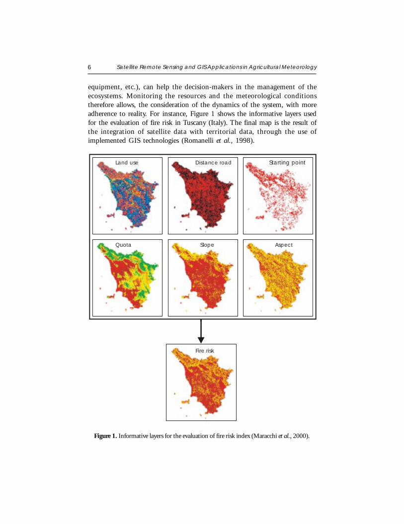
equipment, etc.), can help the decision-makers in the management of theecosystems. Monitoring the resources and the meteorological conditionstherefore allows, the consideration of the dynamics of the system, with moreadherence to reality. For instance, Figure 1 shows the informative layers usedfor the evaluation of fire risk in Tuscany (Italy). The final map is the result ofthe integration of satellite data with territorial data, through the use ofimplemented GIS technologies (Romanelli et al., 1998).
Figure 1. Informative layers for the evaluation of fire risk index (Maracchi et al., 2000).
Land use Distance road Starting point
Quota Slope Aspect
Fire risk
M.V.K. Sivakumar and Donald E. Hinsman 7
These maps of fire risk, constitute a valid tool for foresters and fororganisation of the public services. At the same time, this new informativelayer may be used as the base for other evaluations and simulations. Usingmeteorological data and satellite real-time information, it is possible to diversifythe single situations, advising the competent authorities when the situationmoves to hazard risks. Modelling the ground wind profile and taking intoaccount the meteorological conditions, it is possible to advise the operatorsof the change in the conditions that can directly influence the fire, allowingthe modification of the intervention strategies.
An example of preliminary information system to country scale is givenby the SISP (Integrated information system for monitoring cropping seasonby meteorological and satellite data), developed to allow the monitoring ofthe cropping season and to provide an early warning system with usefulinformation about evolution of crop conditions (Di Chiara and Maracchi,1994). The SISP uses:
Statistical analysis procedures on historical series of rainfall data to produceagroclimatic classification;
A crop (millet) simulation model to estimate millet sowing date and toevaluate the effect of the rainfall distribution on crop growth and yield;
NOAA-NDVI image analysis procedures in order to monitor vegetationcondition;
Analysis procedures of Meteosat images of estimated rainfall for earlyprediction of sowing date and risk areas.
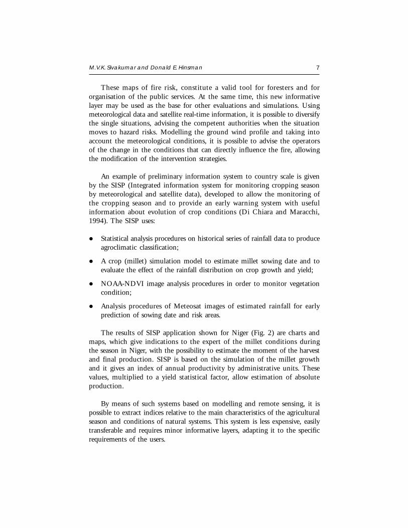
The results of SISP application shown for Niger (Fig. 2) are charts andmaps, which give indications to the expert of the millet conditions duringthe season in Niger, with the possibility to estimate the moment of the harvestand final production. SISP is based on the simulation of the millet growthand it gives an index of annual productivity by administrative units. Thesevalues, multiplied to a yield statistical factor, allow estimation of absoluteproduction.
By means of such systems based on modelling and remote sensing, it ispossible to extract indices relative to the main characteristics of the agriculturalseason and conditions of natural systems. This system is less expensive, easilytransferable and requires minor informative layers, adapting it to the specificrequirements of the users.
8 Satellite Remote Sensing and GIS Applications in Agricultural Meteorology
Figure 2. Examples of outputs of SISP (Maracchi et al., 2000).
SATELLITE REMOTE SENSING
Remote sensing provides spatial coverage by measurement of reflected andemitted electromagnetic radiation, across a wide range of wavebands, from theearth’s surface and surrounding atmosphere. The improvement in technicaltools of meteorological observation, during the last twenty years, has createda favourable substratum for research and monitoring in many applications ofsciences of great economic relevance, such as agriculture and forestry. Eachwaveband provides different information about the atmosphere and landsurface: surface temperature, clouds, solar radiation, processes of photosynthesisand evaporation, which can affect the reflected and emitted radiation, detectedby satellites. The challenge for research therefore is to develop new systemsextracting this information from remotely sensed data, giving to the final users,near-real-time information.
Over the last two decades, the development of space technology has ledto a substantial increase in satellite earth observation systems. Simultaneously,the Information and Communication Technology (ICT) revolution has renderedincreasingly effective the processing of data for specific uses and theirinstantaneous distribution on the World Wide Web (WWW).
The meteorological community and associated environmental disciplinessuch as climatology including global change, hydrology and oceanography allover the world are now able to take advantage of a wealth of observationaldata, products and services flowing from specially equipped and highlysophisticated environmental observation satellites. An environmental
Niamey, cropping season 1993Characterization of land productivity at NigerCeSIA Index for millerElaborated on 10 years (1981-90) and 120 stations
Rainfall Cultural Coeff. Water balanceLongitude

M.V.K. Sivakumar and Donald E. Hinsman 9
observation satellite is an artificial Earth satellite providing data on the Earthsystem and a Meteorological satellite is a type of environmental satelliteproviding meteorological observations. Several factors make environmentalsatellite data unique compared with data from other sources, and it is worthyto note a few of the most important:
Because of its high vantage point and broad field of view, an environmentalsatellite can provide a regular supply of data from those areas of the globeyielding very few conventional observations;
The atmosphere is broadly scanned from satellite altitude and enables large-scale environmental features to be seen in a single view;
The ability of certain satellites to view a major portion of the atmospherecontinually from space makes them particularly well suited for themonitoring and warning of short-lived meteorological phenomena; and
The advanced communication systems developed as an integral part ofthe satellite technology permit the rapid transmission of data from thesatellite, or their relay from automatic stations on earth and in theatmosphere, to operational users.
These factors are incorporated in the design of meteorological satellites toprovide data, products and services through three major functions:
Remote sensing of spectral radiation which can be converted intometeorological measurements such as cloud cover, cloud motion vectors,surface temperature, vertical profiles of atmospheric temperature, humidityand atmospheric constituents such as ozone, snow and ice cover, ozoneand various radiation measurements;
Collection of data from in situ sensors on remote fixed or mobile platformslocated on the earth’s surface or in the atmosphere; and
Direct broadcast to provide cloud-cover images and other meteorologicalinformation to users through a user-operated direct readout station.
The first views of earth from space were not obtained from satellites butfrom converted military rockets in the early 1950s. It was not until 1 April1960 that the first operational meteorological satellite, TIROS-I, was launched
10 Satellite Remote Sensing and GIS Applications in Agricultural Meteorology
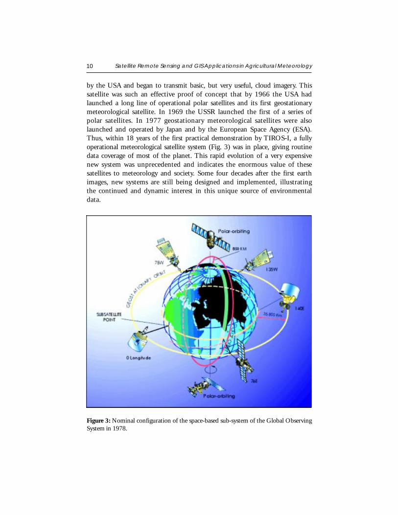
by the USA and began to transmit basic, but very useful, cloud imagery. Thissatellite was such an effective proof of concept that by 1966 the USA hadlaunched a long line of operational polar satellites and its first geostationarymeteorological satellite. In 1969 the USSR launched the first of a series ofpolar satellites. In 1977 geostationary meteorological satellites were alsolaunched and operated by Japan and by the European Space Agency (ESA).Thus, within 18 years of the first practical demonstration by TIROS-I, a fullyoperational meteorological satellite system (Fig. 3) was in place, giving routinedata coverage of most of the planet. This rapid evolution of a very expensivenew system was unprecedented and indicates the enormous value of thesesatellites to meteorology and society. Some four decades after the first earthimages, new systems are still being designed and implemented, illustratingthe continued and dynamic interest in this unique source of environmentaldata.
Figure 3: Nominal configuration of the space-based sub-system of the Global ObservingSystem in 1978.
M.V.K. Sivakumar and Donald E. Hinsman 11
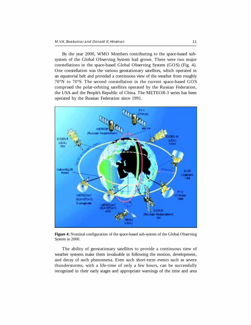
By the year 2000, WMO Members contributing to the space-based sub-system of the Global Observing System had grown. There were two majorconstellations in the space-based Global Observing System (GOS) (Fig. 4).One constellation was the various geostationary satellites, which operated inan equatorial belt and provided a continuous view of the weather from roughly70°N to 70°S. The second constellation in the current space-based GOScomprised the polar-orbiting satellites operated by the Russian Federation,the USA and the People’s Republic of China. The METEOR-3 series has beenoperated by the Russian Federation since 1991.
Figure 4: Nominal configuration of the space-based sub-system of the Global ObservingSystem in 2000.
The ability of geostationary satellites to provide a continuous view ofweather systems make them invaluable in following the motion, development,and decay of such phenomena. Even such short-term events such as severethunderstorms, with a life-time of only a few hours, can be successfullyrecognized in their early stages and appropriate warnings of the time and area
12 Satellite Remote Sensing and GIS Applications in Agricultural Meteorology
of their maximum impact can be expeditiously provided to the general public.For this reason, its warning capability has been the primary justification forthe geostationary spacecraft. Since 71 per cent of the Earth’s surface is waterand even the land areas have many regions which are sparsely inhabited, thepolar-orbiting satellite system provides the data needed to compensate thedeficiencies in conventional observing networks. Flying in a near-polar orbit,the spacecraft is able to acquire data from all parts of the globe in the courseof a series of successive revolutions. For these reasons the polar-orbiting satellitesare principally used to obtain: (a) daily global cloud cover; and (b) accuratequantitative measurements of surface temperature and of the vertical variationof temperature and water vapour in the atmosphere. There is a distinctadvantage in receiving global data acquired by a single set of observing sensors.Together, the polar-orbiting and geostationary satellites constitute a truly globalmeteorological satellite network.
Satellite data provide better coverage in time and in area extent than anyalternative. Most polar satellite instruments observe the entire planet once ortwice in a 24-hour period. Each geostationary satellite’s instruments coverabout ¼ of the planet almost continuously and there are now six geostationarysatellites providing a combined coverage of almost 75%. Satellites cover theworld’s oceans (about 70% of the planet), its deserts, forests, polar regions,and other sparsely inhabited places. Surface winds over the oceans from satellitesare comparable to ship observations; ocean heights can be determined to afew centimetres; and temperatures in any part of the atmosphere anywherein the world are suitable for computer models. It is important to makemaximum use of this information to monitor our environment. Access to thesesatellite data and products is only the beginning. In addition, the ability tointerpret, combine, and make maximum use of this information must be anintegral element of national management in developed and developingcountries.
The thrust of the current generation of environmental satellites is aimedprimarily at characterizing the kinematics and dynamics of the atmosphericcirculation. The existing network of environmental satellites, forming part ofthe GOS of the World Weather Watch produces real-time weather informationon a regular basis. This is acquired several times a day through direct broadcastfrom the meteorological satellites by more than 1,300 stations located in 125countries.
M.V.K. Sivakumar and Donald E. Hinsman 13
The ground segment of the space-based component of the GOS shouldprovide for the reception of signals and DCP data from operational satellitesand/or the processing, formatting and display of meaningful environmentalobservation information, with a view to further distributing it in a convenientform to local users, or over the GTS, as required. This capability is normallyaccomplished through receiving and processing stations of varying complexity,sophistication and cost.
In addition to their current satellite programmes in polar and geostationaryorbits, satellite operators in the USA (NOAA) and Europe (EUMETSAT) haveagreed to launch a series of joint polar-orbiting satellites (METOP) in 2005.These satellites will complement the existing global array of geostationarysatellites that form part of the Global Observing System of the WorldMeteorological Organization. This Initial Joint Polar System (IJPS) representsa major cooperation programme between the USA and Europe in the field ofspace activities. Europe has invested 2 billion Euros in a low earth orbit satellitesystem, which will be available operationally from 2006 to 2020.
The data provided by these satellites will enable development ofoperational services in improved temperature and moisture sounding fornumerical weather prediction (NWP), tropospheric/stratospheric interactions,imagery of clouds and land/ocean surfaces, air-sea interactions, ozone and othertrace gases mapping and monitoring, and direct broadcast support tonowcasting. Advanced weather prediction models are needed to assimilatesatellite information at the highest possible spatial and spectral resolutions.It imposes new requirements on the precision and spectral resolution ofsoundings in order to improve the quality of weather forecasts. Satelliteinformation is already used by fishery-fleets on an operational basis. Windand the resulting surface stress is the major force for oceanic motions. Oceancirculation forecasts require the knowledge of an accurate wind field. Windmeasurements from space play an increasing role in monitoring of climatechange and variability. The chemical composition of the troposphere ischanging on all spatial scales. Increases in trace gases with long atmosphericresidence times can affect the climate and chemical equilibrium of the Earth/Atmosphere system. Among these trace gases are methane, nitrogen dioxide,and ozone. The chemical and dynamic state of the stratosphere influence thetroposphere by exchange processes through the tropopause. Continuousmonitoring of ozone and of (the main) trace gases in the troposphere and thestratosphere is an essential input to the understanding of the relatedatmospheric chemistry processes.
14 Satellite Remote Sensing and GIS Applications in Agricultural Meteorology
WMO SPACE PROGRAMME
The World Meteorological Organization, a specialized agency of the UnitedNations, has a membership of 187 states and territories (as of June 2003).Amongst the many programmes and activities of the organization, there arethree areas which are particularly pertinent to the satellite activities:
To facilitate world-wide cooperation in the establishment of networks formaking meteorological, as well as hydrological and other geophysicalobservations and centres to provide meteorological services;
To promote the establishment and maintenance of systems for the rapidexchange of meteorological and related information;
To promote the standardization of meteorological observations and ensurethe uniform publication of observations and statistics.
The Fourteenth WMO Congress, held in May 2003, initiated a new MajorProgramme, the WMO Space Programme, as a cross-cutting programme toincrease the effectiveness and contributions from satellite systems to WMOProgrammes. Congress recognized the critical importance for data, productsand services provided by the World Weather Watch’s (WWW) expanded space-based component of the Global Observing System (GOS) to WMOProgrammes and supported Programmes. During the past four years, the useby WMO Members of satellite data, products and services has experiencedtremendous growth to the benefit of almost all WMO Programmes andsupported Programmes. The decision by the fifty-third Executive Council toexpand the space-based component of the Global Observing System to includeappropriate R&D environmental satellite missions was a landmark decisionin the history of WWW. Congress agreed that the Commission for BasicSystems (CBS) should continue the lead role in full consultation with the othertechnical commissions for the new WMO Space Programme. Congress alsodecided to establish WMO Consultative Meetings on High-level Policy onSatellite Matters. The Consultative Meetings will provide advice and guidanceon policy-related matters and maintain a high level overview of the WMOSpace Programme. The expected benefits from the new WMO SpaceProgramme include an increasing contribution to the development of theWWW’s GOS, as well as to the other WMO-supported programmes andassociated observing systems through the provision of continuously improveddata, products and services, from both operational and R&D satellites, and
M.V.K. Sivakumar and Donald E. Hinsman 15
to facilitate and promote their wider availability and meaningful utilizationaround the globe.
The main thrust of the WMO Space Programme Long-term Strategy is:
“To make an increasing contribution to the development of the WWW’sGOS, as well as to the other WMO-supported Programmes and associatedobserving systems (such as AREP’s GAW, GCOS, WCRP, HWR’s WHYCOSand JCOMM’s implementation of GOS) through the provision of continuouslyimproved data, products and services, from both operational and R&Dsatellites, and to facilitate and promote their wider availability and meaningfulutilization around the globe”.
The main elements of the WMO Space Programme Long-term Strategyare as follows:
(a) Increased involvement of space agencies contributing, or with thepotential to contribute to, the space-based component of the GOS;
(b) Promotion of a wider awareness of the availability and utilization ofdata, products - and their importance at levels 1, 2, 3 or 4 - andservices, including those from R&D satellites;
(c) Considerably more attention to be paid to the crucial problemsconnected with the assimilation of R&D and new operational datastreams in nowcasting, numerical weather prediction systems,reanalysis projects, monitoring climate change, chemical compositionof the atmosphere, as well as the dominance of satellite data in somecases;
(d) Closer and more effective cooperation with relevant internationalbodies;
(e) Additional and continuing emphasis on education and training;
(f ) Facilitation of the transition from research to operational systems;
(g) Improved integration of the space component of the various observingsystems throughout WMO Programmes and WMO-supportedProgrammes;
16 Satellite Remote Sensing and GIS Applications in Agricultural Meteorology
(h) Increased cooperation amongst WMO Members to develop commonbasic tools for utilization of research, development and operationalremote sensing systems.
Coordination Group for Meteorological Satellites (CGMS)
In 1972 a group of satellite operators formed the Co-ordination ofGeostationary Meteorological Satellites (CGMS) that would be expanded inthe early 1990s to include polar-orbiting satellites and changed its name -but not its abbreviation - to the Co-ordination Group for MeteorologicalSatellites. The Co-ordination Group for Meteorological Satellites (CGMS)provides a forum for the exchange of technical information on geostationaryand polar orbiting meteorological satellite systems, such as reporting on currentmeteorological satellite status and future plans, telecommunication matters,operations, inter-calibration of sensors, processing algorithms, products andtheir validation, data transmission formats and future data transmissionstandards.
Since 1972, the CGMS has provided a forum in which the satelliteoperators have studied jointly with the WMO technical operational aspectsof the global network, so as to ensure maximum efficiency and usefulnessthrough proper coordination in the design of the satellites and in theprocedures for data acquisition and dissemination.
Membership of CGMS
The table of members shows the lead agency in each case. Delegates are oftensupported by other agencies, for example, ESA (with EUMETSAT), NASDA(with Japan) and NASA (with NOAA).
The current Membership of CGMS is:
EUMETSAT joined 1987currently CGMS Secretariat
India Meteorological Department joined 1979
Japan Meteorological Agency founder member, 1972
China Meteorological Administration joined 1989
NOAA/NESDIS founder member, 1972
Hydromet Service of the Russian Federation joined 1973
M.V.K. Sivakumar and Donald E. Hinsman 17
WMO joined 1973
IOC of UNESCO joined 2000
NASA joined 2002
ESA joined 2002
NASDA joined 2002
Rosaviakosmos joined 2002
WMO, in its endeavours to promote the development of a globalmeteorological observing system, participated in the activities of CGMS fromits first meeting. There are several areas where joint consultations between thesatellite operators and WMO are needed. The provision of data tometeorological centres in different parts of the globe is achieved by means ofthe Global Telecommunication System (GTS) in near-real-time. Thisautomatically involves assistance by WMO in developing appropriate codeforms and provision of a certain amount of administrative communicationsbetween the satellite operators.
WMO’s role within CGMS would be to state the observational and systemrequirements for WMO and supported programmes as they relate to theexpanded space-based components of the GOS, GAW, GCOS and WHYCOS.CGMS satellite operators would make their voluntary commitments to meetthe stated observational and system requirements. WMO would, through itsMembers, strive to provide CGMS satellite operators with operational and pre-operational evaluations of the benefit and impacts of their satellite systems.WMO would also act as a catalyst to foster direct user interactions with theCGMS satellite operators through available means such as conferences,symposia and workshops.
The active involvement of WMO has allowed the development andimplementation of the operational ASDAR system as a continuing part of theGlobal Observing System. Furthermore, the implementation of the IDCSsystem was promoted by WMO and acted jointly with the satellite operatorsas the admitting authority in the registration procedure for IDCPs.
The expanded space-based component of the world weather watch’s globalobserving system
Several initiatives since 2000 with regard to WMO satellite activities haveculminated in an expansion of the space-based component of the Global
18 Satellite Remote Sensing and GIS Applications in Agricultural Meteorology
Observing System to include appropriate Research and Development (R&D)satellite missions. The recently established WMO Consultative Meetings onHigh-Level Policy on Satellite Matters have acted as a catalyst in each of theseinterwoven and important areas. First was the establishment of a new seriesof technical documents on the operational use of R&D satellite data. Secondwas a recognition of the importance of R&D satellite data in meeting WMOobservational data requirements and the subsequent development of a set ofGuidelines for requirements for observational data from operational and R&Dsatellite missions. Third have been the responses by the R&D space agenciesin making commitments in support of the system design for the space-basedcomponent of the Global Observing System. And lastly has been WMO’srecognition that it should have a more appropriate programme structure - aWMO Space Programme - to capitalize on the full potential of satellite data,products and services from both the operational and R&D satellites.
WMO Members’ responses to the request for input for the report on theutility of R&D satellite data and products covered the full spectrum of WMORegions as well as a good cross-section of developed and developing countries.Countries from both the Northern and Southern Hemispheres, tropical, mid-and high-latitude as well as those with coastlines and those landlocked hadresponded. Most disciplines and application areas including NWP, hydrology,climate, oceanography, agrometeorology, environmental monitoring anddetection and monitoring of natural disasters were included.
A number of WMO Programmes and associated application areassupported by data and products from the R&D satellites. While not complete,the list included specific applications within the disciplines of agrometeorology,weather forecasting, hydrology, climate and oceanography including:monitoring of ecology, sea-ice, snow cover, urban heat island, crop yield,vegetation, flood, volcanic ash and other natural disasters; tropical cycloneforecasting; fire areas; oceanic chlorophyll content; NWP; sea height; and CO
2
exchange between the atmosphere and ocean.
WMO agreed that there was an increasing convergence between researchand operational requirements for the space-based component of the GlobalObserving System and that WMO should seek to establish a continuum ofrequirements for observational data from R&D satellite missions to operationalmissions. WMO endorsed the Guidelines for requirements for observational datafrom operational and R&D satellite missions to provide operational users ameasure of confidence in the availability of operational and R&D observationaldata, and data providers with an indication of its utility.
M.V.K. Sivakumar and Donald E. Hinsman 19
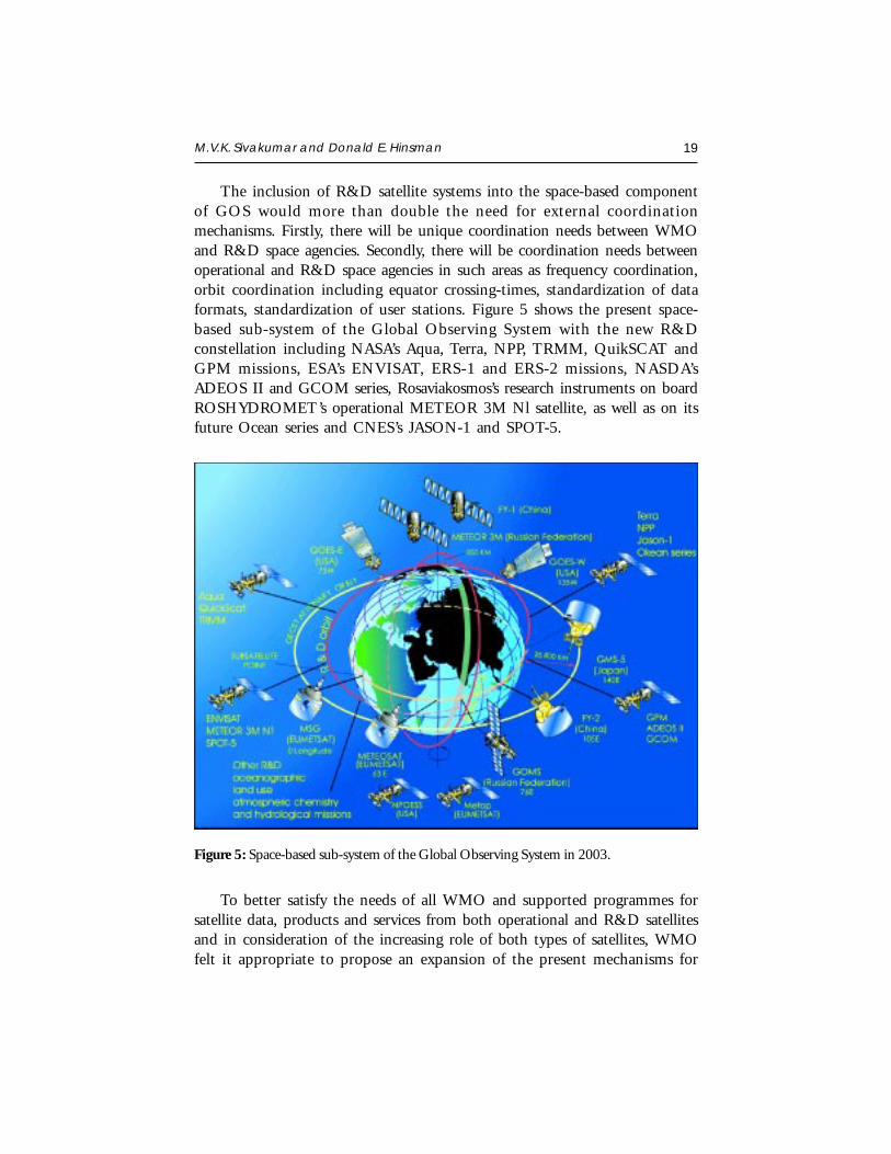
The inclusion of R&D satellite systems into the space-based componentof GOS would more than double the need for external coordinationmechanisms. Firstly, there will be unique coordination needs between WMOand R&D space agencies. Secondly, there will be coordination needs betweenoperational and R&D space agencies in such areas as frequency coordination,orbit coordination including equator crossing-times, standardization of dataformats, standardization of user stations. Figure 5 shows the present space-based sub-system of the Global Observing System with the new R&Dconstellation including NASA’s Aqua, Terra, NPP, TRMM, QuikSCAT andGPM missions, ESA’s ENVISAT, ERS-1 and ERS-2 missions, NASDA’sADEOS II and GCOM series, Rosaviakosmos’s research instruments on boardROSHYDROMET’s operational METEOR 3M Nl satellite, as well as on itsfuture Ocean series and CNES’s JASON-1 and SPOT-5.
Figure 5: Space-based sub-system of the Global Observing System in 2003.
To better satisfy the needs of all WMO and supported programmes forsatellite data, products and services from both operational and R&D satellitesand in consideration of the increasing role of both types of satellites, WMOfelt it appropriate to propose an expansion of the present mechanisms for
20 Satellite Remote Sensing and GIS Applications in Agricultural Meteorology
coordination within the WMO structure and cooperation between WMO andthe operators of operational meteorological satellites and R&D satellites. Indoing so, WMO felt that an effective means to improve cooperation with bothoperational meteorological and R&D satellite operators would be through anexpanded CGMS that would include those R&D space agencies contributingto the space-based component of the GOS.
WMO agreed that the WMO satellite activities had grown and that itwas now appropriate to establish a WMO Space Programme as a matter ofpriority. The scope, goals and objectives of the new programme should respondto the tremendous growth in the utilization of environmental satellite data,products and services within the expanded space-based component of the GOSthat now include appropriate Research and Development environmentalsatellite missions. The Consultative Meetings on High-Level Policy on SatelliteMatters should be institutionalized in order to more formally establish thedialogue and participation of environmental satellite agencies in WMO matters.In considering the important contributions made by environmental satellitesystems to WMO and its supported programmes as well as the largeexpenditures by the space agencies, WMO felt it appropriate that the overallresponsibility for the new WMO Space Programme should be assigned to CBSand a new institutionalized Consultative Meetings on High-Level Policy onSatellite Matters.
CONCLUSIONS
Recent developments in remote sensing and GIS hold much promise toenhance integrated management of all available information and the extractionof desired information to promote sustainable agriculture and development.Active promotion of the use of remote sensing and GIS in the NationalMeteorological and Hydrological Services (NMHSs), could enhance improvedagrometeorological applications. To this end it is important to reinforce trainingin these new fields. The promotion of new specialised software should makethe applications of the various devices easier, bearing in mind the possiblecombination of several types of inputs such as data coming from standardnetworks, radar and satellites, meteorological and climatological models, digitalcartography and crop models based on the scientific acquisition of the lasttwenty years. International cooperation is crucial to promote the much neededapplications in the developing countries and the WMO Space Programmeactively promotes such cooperation throughout all WMO Programmes andprovides guidance to these and other multi-sponsored programmes on thepotential of remote sensing techniques in meteorology, hydrology and related
M.V.K. Sivakumar and Donald E. Hinsman 21
disciplines, as well as in their applications. The new WMO Space Programmewill further enhance both external and internal coordination necessary tomaximize the exploitation of the space-based component of the GOS to providevaluable satellite data, products and services to WMO Members towardsmeeting observational data requirements for WMO programmes more so thanever before in the history of the World Weather Watch.
REFERENCES
Di Chiara, C. and G. Maracchi. 1994. Guide au S.I.S.P. ver. 1.0. Technical Manual No. 14,CeSIA, Firenze, Italy.
Kleschenko, A.D. 1983. Use of remote sensing for obtaining agrometeorological information.CAgM Report No. 12, Part I. Geneva, Switzerland: World Meteorological Organization.
Kanemasu, E.T. and I.D. Filcroft. 1992. Operational remote sensing systems in agriculture.CAgM Report No. 50, Part I. Geneva, Switzerland: World Meteorological Organization.
Maracchi, G. 1991. Agrometeorologia : stato attuale e prospettive future. Proc. CongressAgrometeorologia e Telerilevamento. Agronica, Palermo, Italy, pp. 1-5.
Maracchi, G., V. Pérarnaud and A.D. Kleschenko. 2000. Applications of geographicalinformation systems and remote sensing in agrometeorology. Agric. For. Meteorol.103:119-136.
Romanelli, S., L. Bottai and F. Maselli. 1998. Studio preliminare per la stima del rischiod’incendio boschivo a scala regionale per mezzo dei dati satellitari e ausilari. TuscanyRegion - Laboratory for Meteorology and Environmental Modelling (LaMMA), Firenze,Italy.
Seguin, B. 1992. Satellite applications to agrometeorology: technological developments forthe period 1985-1989. CAgM Report No. 50, Part II. Geneva, Switzerland: WorldMeteorological Organization.
Seitnazarov, 1999. Technology and methods of collection, distribution and analyzing ofagrometeorological data in Dashhovuz velajat, Turkmenistan. In: Contributions frommembers on Operational Applications in the International Workshop onAgrometeorology in the 21st Century: Needs and Perspectives, Accra, Ghana. CAgMReport No. 77, Geneva, Switzerland: World Meteorological Organization.
WMO. 1998. Preliminary statement of guidance regarding how well satellite capabilitiesmeet WMO user requirements in several application areas, SAT-21, WMO/TD No.913, Geneva, Switzerland: World Meteorological Organization.
WMO. 2000. Statement of guidance regarding how well satellite capabilities meet wmouser requirements in several application areas. SAT-22, WMO/TD No. 992, Geneva,Switzerland: World Meteorological Organization.
PRINCIPLES OF REMOTE SENSING
Shefali AggarwalPhotogrammetry and Remote Sensing DivisionIndian Institute of Remote Sensing, Dehra Dun
Abstract : Remote sensing is a technique to observe the earth surface or theatmosphere from out of space using satellites (space borne) or from the air usingaircrafts (airborne). Remote sensing uses a part or several parts of theelectromagnetic spectrum. It records the electromagnetic energy reflected or emittedby the earth’s surface. The amount of radiation from an object (called radiance) isinfluenced by both the properties of the object and the radiation hitting the object(irradiance). The human eyes register the solar light reflected by these objects andour brains interpret the colours, the grey tones and intensity variations. In remotesensing various kinds of tools and devices are used to make electromagnetic radiationoutside this range from 400 to 700 nm visible to the human eye, especially thenear infrared, middle-infrared, thermal-infrared and microwaves.
Remote sensing imagery has many applications in mapping land-use and cover,agriculture, soils mapping, forestry, city planning, archaeological investigations,military observation, and geomorphological surveying, land cover changes,deforestation, vegetation dynamics, water quality dynamics, urban growth, etc. Thispaper starts with a brief historic overview of remote sensing and then explains the
various stages and the basic principles of remotely sensed data collection mechanism.
INTRODUCTION
Remote sensing (RS), also called earth observation, refers to obtaininginformation about objects or areas at the Earth’s surface without being
in direct contact with the object or area. Humans accomplish this task withaid of eyes or by the sense of smell or hearing; so, remote sensing is day-to-day business for people. Reading the newspaper, watching cars driving in frontof you are all remote sensing activities. Most sensing devices record informationabout an object by measuring an object’s transmission of electromagnetic energyfrom reflecting and radiating surfaces.
Satellite Remote Sensing and GIS Applications in Agricultural Meteorologypp. 23-38
24 Principles of Remote Sensing
Remote sensing techniques allow taking images of the earth surface invarious wavelength region of the electromagnetic spectrum (EMS). One of themajor characteristics of a remotely sensed image is the wavelength region itrepresents in the EMS. Some of the images represent reflected solar radiationin the visible and the near infrared regions of the electromagnetic spectrum,others are the measurements of the energy emitted by the earth surface itselfi.e. in the thermal infrared wavelength region. The energy measured in themicrowave region is the measure of relative return from the earth’s surface,where the energy is transmitted from the vehicle itself. This is known as activeremote sensing, since the energy source is provided by the remote sensingplatform. Whereas the systems where the remote sensing measurementsdepend upon the external energy source, such as sun are referred to as passiveremote sensing systems.
PRINCIPLES OF REMOTE SENSING
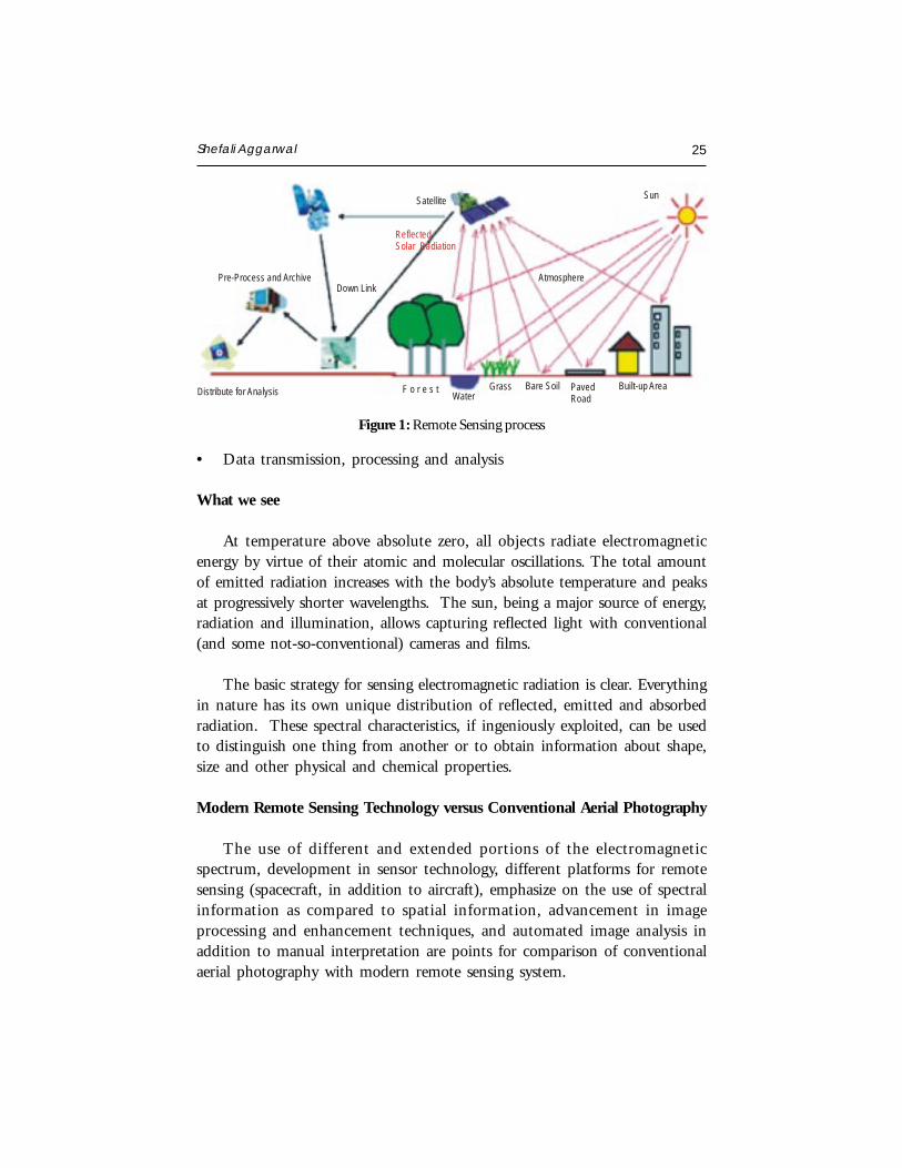
Detection and discrimination of objects or surface features means detectingand recording of radiant energy reflected or emitted by objects or surfacematerial (Fig. 1). Different objects return different amount of energy in differentbands of the electromagnetic spectrum, incident upon it. This depends onthe property of material (structural, chemical, and physical), surface roughness,angle of incidence, intensity, and wavelength of radiant energy.
The Remote Sensing is basically a multi-disciplinary science which includesa combination of various disciplines such as optics, spectroscopy, photography,computer, electronics and telecommunication, satellite launching etc. All thesetechnologies are integrated to act as one complete system in itself, known asRemote Sensing System. There are a number of stages in a Remote Sensingprocess, and each of them is important for successful operation.
Stages in Remote Sensing
• Emission of electromagnetic radiation, or EMR (sun/self- emission)
• Transmission of energy from the source to the surface of the earth, as wellas absorption and scattering
• Interaction of EMR with the earth’s surface: reflection and emission
• Transmission of energy from the surface to the remote sensor
• Sensor data output
Shefali Aggarwal 25
• Data transmission, processing and analysis
What we see
At temperature above absolute zero, all objects radiate electromagneticenergy by virtue of their atomic and molecular oscillations. The total amountof emitted radiation increases with the body’s absolute temperature and peaksat progressively shorter wavelengths. The sun, being a major source of energy,radiation and illumination, allows capturing reflected light with conventional(and some not-so-conventional) cameras and films.
The basic strategy for sensing electromagnetic radiation is clear. Everythingin nature has its own unique distribution of reflected, emitted and absorbedradiation. These spectral characteristics, if ingeniously exploited, can be usedto distinguish one thing from another or to obtain information about shape,size and other physical and chemical properties.
Modern Remote Sensing Technology versus Conventional Aerial Photography
The use of different and extended portions of the electromagneticspectrum, development in sensor technology, different platforms for remotesensing (spacecraft, in addition to aircraft), emphasize on the use of spectralinformation as compared to spatial information, advancement in imageprocessing and enhancement techniques, and automated image analysis inaddition to manual interpretation are points for comparison of conventionalaerial photography with modern remote sensing system.
Figure 1: Remote Sensing process
Built-up Area
Sun
Distribute for Analysis
Pre-Process and Archive
Satellite
ReflectedSolar Radiation
F o r e s t GrassWater
Bare Soil Paved Road
AtmosphereDown Link
26 Principles of Remote Sensing
During early half of twentieth century, aerial photos were used in militarysurveys and topographical mapping. Main advantage of aerial photos has beenthe high spatial resolution with fine details and therefore they are still usedfor mapping at large scale such as in route surveys, town planning,construction project surveying, cadastral mapping etc. Modern remote sensingsystem provide satellite images suitable for medium scale mapping used innatural resources surveys and monitoring such as forestry, geology, watershedmanagement etc. However the future generation satellites are going to providemuch high-resolution images for more versatile applications.
HISTORIC OVERVIEW
In 1859 Gaspard Tournachon took an oblique photograph of a small villagenear Paris from a balloon. With this picture the era of earth observation andremote sensing had started. His example was soon followed by other peopleall over the world. During the Civil War in the United States aerialphotography from balloons played an important role to reveal the defencepositions in Virginia (Colwell, 1983). Likewise other scientific and technicaldevelopments this Civil War time in the United States speeded up thedevelopment of photography, lenses and applied airborne use of thistechnology. Table 1 shows a few important dates in the development of remotesensing.
The next period of fast development took place in Europe and not in theUnited States. It was during World War I that aero planes were used on alarge scale for photoreconnaissance. Aircraft proved to be more reliable andmore stable platforms for earth observation than balloons. In the periodbetween World War I and World War II a start was made with the civilianuse of aerial photos. Application fields of airborne photos included at thattime geology, forestry, agriculture and cartography. These developments leadto much improved cameras, films and interpretation equipment. The mostimportant developments of aerial photography and photo interpretation tookplace during World War II. During this time span the development of otherimaging systems such as near-infrared photography; thermal sensing and radartook place. Near-infrared photography and thermal-infrared proved veryvaluable to separate real vegetation from camouflage. The first successfulairborne imaging radar was not used for civilian purposes but proved valuablefor nighttime bombing. As such the system was called by the military ‘planposition indicator’ and was developed in Great Britain in 1941.
Shefali Aggarwal 27
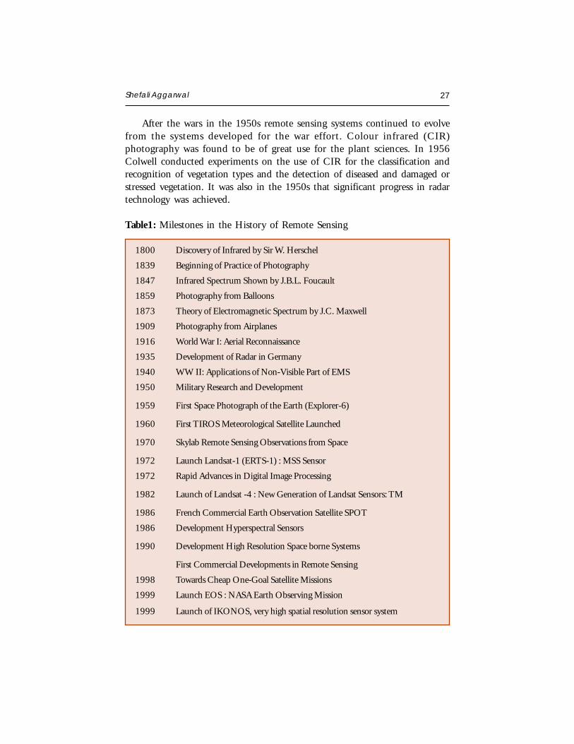
After the wars in the 1950s remote sensing systems continued to evolvefrom the systems developed for the war effort. Colour infrared (CIR)photography was found to be of great use for the plant sciences. In 1956Colwell conducted experiments on the use of CIR for the classification andrecognition of vegetation types and the detection of diseased and damaged orstressed vegetation. It was also in the 1950s that significant progress in radartechnology was achieved.
Table1: Milestones in the History of Remote Sensing
1800 Discovery of Infrared by Sir W. Herschel
1839 Beginning of Practice of Photography
1847 Infrared Spectrum Shown by J.B.L. Foucault
1859 Photography from Balloons
1873 Theory of Electromagnetic Spectrum by J.C. Maxwell
1909 Photography from Airplanes
1916 World War I: Aerial Reconnaissance
1935 Development of Radar in Germany
1940 WW II: Applications of Non-Visible Part of EMS
1950 Military Research and Development
1959 First Space Photograph of the Earth (Explorer-6)
1960 First TIROS Meteorological Satellite Launched
1970 Skylab Remote Sensing Observations from Space
1972 Launch Landsat-1 (ERTS-1) : MSS Sensor
1972 Rapid Advances in Digital Image Processing
1982 Launch of Landsat -4 : New Generation of Landsat Sensors: TM
1986 French Commercial Earth Observation Satellite SPOT
1986 Development Hyperspectral Sensors
1990 Development High Resolution Space borne Systems
First Commercial Developments in Remote Sensing
1998 Towards Cheap One-Goal Satellite Missions
1999 Launch EOS : NASA Earth Observing Mission
1999 Launch of IKONOS, very high spatial resolution sensor system
28 Principles of Remote Sensing
ELECTROMAGNETIC RADIATION AND THE ELECTROMAGNETICSPECTRUM
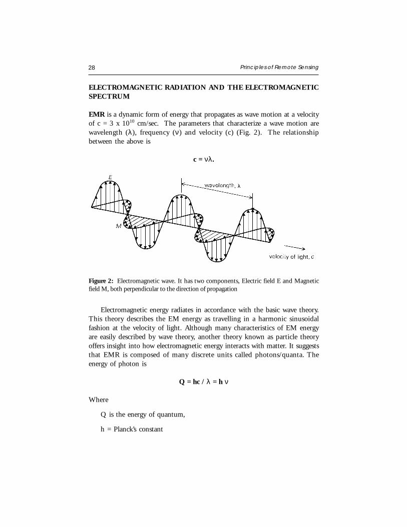
EMR is a dynamic form of energy that propagates as wave motion at a velocityof c = 3 x 1010 cm/sec. The parameters that characterize a wave motion arewavelength (λ), frequency (ν) and velocity (c) (Fig. 2). The relationshipbetween the above is
c = νλ .
Figure 2: Electromagnetic wave. It has two components, Electric field E and Magneticfield M, both perpendicular to the direction of propagation
Electromagnetic energy radiates in accordance with the basic wave theory.This theory describes the EM energy as travelling in a harmonic sinusoidalfashion at the velocity of light. Although many characteristics of EM energyare easily described by wave theory, another theory known as particle theoryoffers insight into how electromagnetic energy interacts with matter. It suggeststhat EMR is composed of many discrete units called photons/quanta. Theenergy of photon is
Q = hc / λ = h ν
Where
Q is the energy of quantum,
h = Planck’s constant
Shefali Aggarwal 29
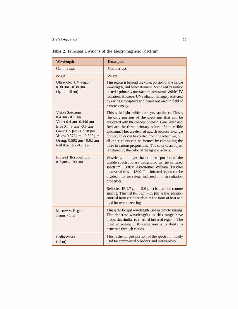
This region is beyond the violet portion of the visiblewavelength, and hence its name. Some earth’s surfacematerial primarily rocks and minerals emit visible UVradiation. However UV radiation is largely scatteredby earth’s atmosphere and hence not used in field ofremote sensing.
This is the light, which our eyes can detect. This isthe only portion of the spectrum that can beassociated with the concept of color. Blue Green andRed are the three primary colors of the visiblespectrum. They are defined as such because no singleprimary color can be created from the other two, butall other colors can be formed by combining thethree in various proportions. The color of an objectis defined by the color of the light it reflects.
Wavelengths longer than the red portion of thevisible spectrum are designated as the infraredspectrum. British Astronomer William Herscheldiscovered this in 1800. The infrared region can bedivided into two categories based on their radiationproperties.
Reflected IR (.7 µm - 3.0 µm) is used for remotesensing. Thermal IR (3 µm - 35 µm) is the radiationemitted from earth’s surface in the form of heat andused for remote sensing.
This is the longest wavelength used in remote sensing.The shortest wavelengths in this range haveproperties similar to thermal infrared region. Themain advantage of this spectrum is its ability topenetrate through clouds.
This is the longest portion of the spectrum mostlyused for commercial broadcast and meteorology.
Table 2: Principal Divisions of the Electromagnetic Spectrum
Wavelength Description
Gamma rays Gamma rays
X-rays X-rays
Ultraviolet (UV) region0.30 µm - 0.38 µm(1µm = 10-6m)
Visible Spectrum0.4 µm - 0.7 µmViolet 0.4 µm -0.446 µmBlue 0.446 µm -0.5 µmGreen 0.5 µm - 0.578 µmYellow 0.578 µm - 0.592 µmOrange 0.592 µm - 0.62 µmRed 0.62 µm -0.7 µm
Infrared (IR) Spectrum0.7 µm – 100 µm
Microwave Region1 mm - 1 m
Radio Waves(>1 m)
30 Principles of Remote Sensing
Types of Remote Sensing
Remote sensing can be either passive or active. ACTIVE systems have theirown source of energy (such as RADAR) whereas the PASSIVE systems dependupon external source of illumination (such as SUN) or self-emission for remotesensing.
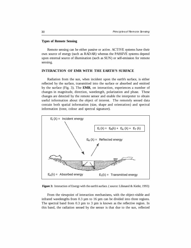
INTERACTION OF EMR WITH THE EARTH’S SURFACE
Radiation from the sun, when incident upon the earth’s surface, is eitherreflected by the surface, transmitted into the surface or absorbed and emittedby the surface (Fig. 3). The EMR, on interaction, experiences a number ofchanges in magnitude, direction, wavelength, polarization and phase. Thesechanges are detected by the remote sensor and enable the interpreter to obtainuseful information about the object of interest. The remotely sensed datacontain both spatial information (size, shape and orientation) and spectralinformation (tone, colour and spectral signature).
Figure 3: Interaction of Energy with the earth’s surface. ( source: Liliesand & Kiefer, 1993)
From the viewpoint of interaction mechanisms, with the object-visible andinfrared wavelengths from 0.3 µm to 16 µm can be divided into three regions.The spectral band from 0.3 µm to 3 µm is known as the reflective region. Inthis band, the radiation sensed by the sensor is that due to the sun, reflected
ER (λ) = Reflected energy
EI (λ) = ER(λ) + EA (λ) + ET (λ)
EI (λ) = Incident energy
EA(λ) = Absorbed energy ET(λ) = Transmitted energy
Shefali Aggarwal 31
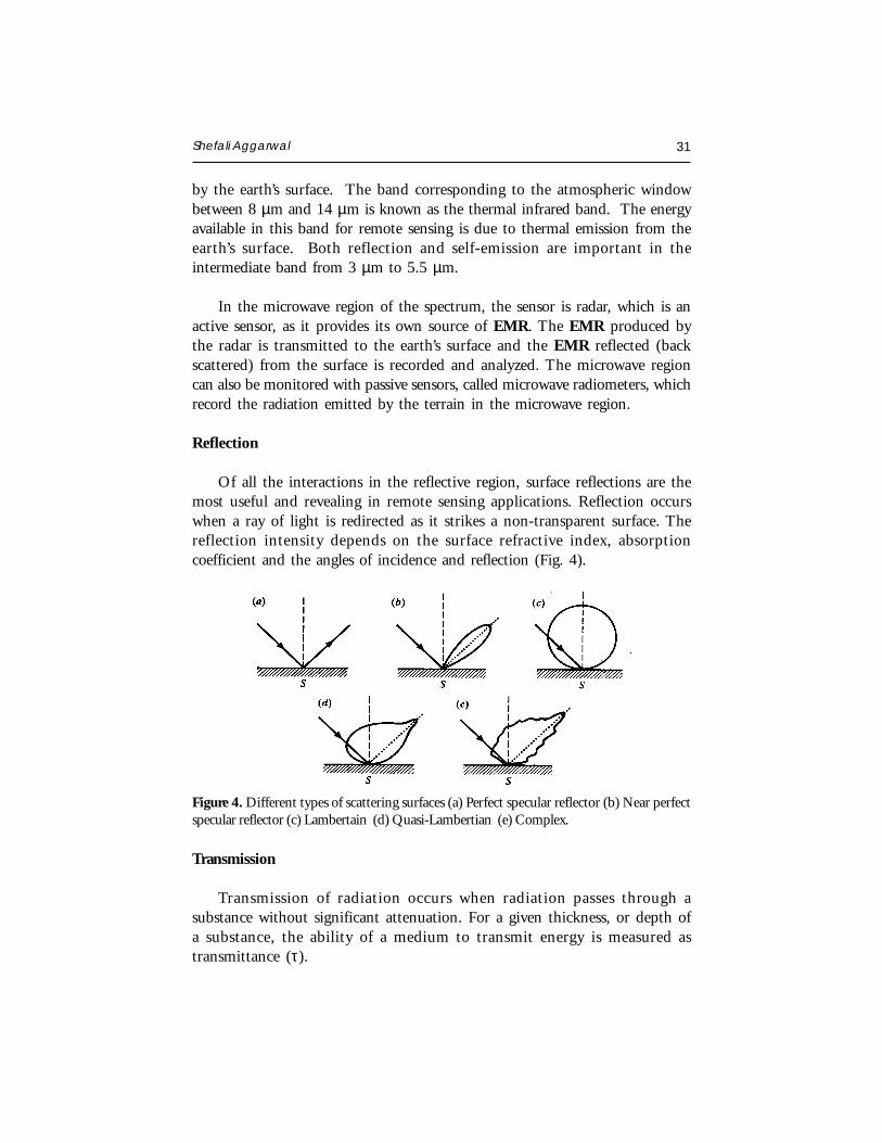
Figure 4. Different types of scattering surfaces (a) Perfect specular reflector (b) Near perfectspecular reflector (c) Lambertain (d) Quasi-Lambertian (e) Complex.
by the earth’s surface. The band corresponding to the atmospheric windowbetween 8 µm and 14 µm is known as the thermal infrared band. The energyavailable in this band for remote sensing is due to thermal emission from theearth’s surface. Both reflection and self-emission are important in theintermediate band from 3 µm to 5.5 µm.
In the microwave region of the spectrum, the sensor is radar, which is anactive sensor, as it provides its own source of EMR. The EMR produced bythe radar is transmitted to the earth’s surface and the EMR reflected (backscattered) from the surface is recorded and analyzed. The microwave regioncan also be monitored with passive sensors, called microwave radiometers, whichrecord the radiation emitted by the terrain in the microwave region.
Reflection
Of all the interactions in the reflective region, surface reflections are themost useful and revealing in remote sensing applications. Reflection occurswhen a ray of light is redirected as it strikes a non-transparent surface. Thereflection intensity depends on the surface refractive index, absorptioncoefficient and the angles of incidence and reflection (Fig. 4).
Transmission
Transmission of radiation occurs when radiation passes through asubstance without significant attenuation. For a given thickness, or depth ofa substance, the ability of a medium to transmit energy is measured astransmittance (τ).
32 Principles of Remote Sensing
Transmitted radiationτ =———————————
Incident radiation
Spectral Signature
Spectral reflectance, [ρ(λ)], is the ratio of reflected energy to incidentenergy as a function of wavelength. Various materials of the earth’s surface havedifferent spectral reflectance characteristics. Spectral reflectance is responsiblefor the color or tone in a photographic image of an object. Trees appear greenbecause they reflect more of the green wavelength. The values of the spectralreflectance of objects averaged over different, well-defined wavelength intervalscomprise the spectral signature of the objects or features by which they canbe distinguished. To obtain the necessary ground truth for the interpretationof multispectral imagery, the spectral characteristics of various natural objectshave been extensively measured and recorded.
The spectral reflectance is dependent on wavelength, it has different valuesat different wavelengths for a given terrain feature. The reflectancecharacteristics of the earth’s surface features are expressed by spectral reflectance,which is given by:
ρ(λ) = [ER(λ) / EI(λ)] x 100
Where,
ρ(λ) = Spectral reflectance (reflectivity) at a particular wavelength.
ER(λ) = Energy of wavelength reflected from object
EI(λ) = Energy of wavelength incident upon the object
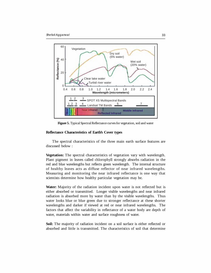
The plot between ρ(λ) and λ is called a spectral reflectance curve. Thisvaries with the variation in the chemical composition and physical conditionsof the feature, which results in a range of values. The spectral response patternsare averaged to get a generalized form, which is called generalized spectralresponse pattern for the object concerned. Spectral signature is a term usedfor unique spectral response pattern, which is characteristic of a terrain feature.Figure 5 shows a typical reflectance curves for three basic types of earth surfacefeatures, healthy vegetation, dry bare soil (grey-brown and loamy) and clearlake water.
Shefali Aggarwal 33
Reflectance Characteristics of Earth’s Cover types
The spectral characteristics of the three main earth surface features arediscussed below :
Vegetation: The spectral characteristics of vegetation vary with wavelength.Plant pigment in leaves called chlorophyll strongly absorbs radiation in thered and blue wavelengths but reflects green wavelength. The internal structureof healthy leaves acts as diffuse reflector of near infrared wavelengths.Measuring and monitoring the near infrared reflectance is one way thatscientists determine how healthy particular vegetation may be.
Water: Majority of the radiation incident upon water is not reflected but iseither absorbed or transmitted. Longer visible wavelengths and near infraredradiation is absorbed more by water than by the visible wavelengths. Thuswater looks blue or blue green due to stronger reflectance at these shorterwavelengths and darker if viewed at red or near infrared wavelengths. Thefactors that affect the variability in reflectance of a water body are depth ofwater, materials within water and surface roughness of water.
Soil: The majority of radiation incident on a soil surface is either reflected orabsorbed and little is transmitted. The characteristics of soil that determine
Figure 5. Typical Spectral Reflectance curves for vegetation, soil and water
VegetationDry soil(5% water)
Wet soil(20% water)
Clear lake waterTurbid river water
0.4 0.6 0.8 1.0 1.2 1.4 1.6 1.8 2.0 2.2 2.4Wavelength (micrometers)
SPOT XS Multispectral Bands
Landsat TM Bands 5 7
1 2 3
1 2 3 4
60
40
20
0
Middle InfraredReflected Infrared
Ref
lect
ance
(%)
34 Principles of Remote Sensing
its reflectance properties are its moisture content, organic matter content,texture, structure and iron oxide content. The soil curve shows less peak andvalley variations. The presence of moisture in soil decreases its reflectance.
By measuring the energy that is reflected by targets on earth’s surface overa variety of different wavelengths, we can build up a spectral signature forthat object. And by comparing the response pattern of different features wemay be able to distinguish between them, which we may not be able to do ifwe only compare them at one wavelength. For example, Water and Vegetationreflect somewhat similarly in the visible wavelength but not in the infrared.
INTERACTIONS WITH THE ATMOSPHERE
The sun is the source of radiation, and electromagnetic radiation (EMR)from the sun that is reflected by the earth and detected by the satellite oraircraft-borne sensor must pass through the atmosphere twice, once on itsjourney from the sun to the earth and second after being reflected by thesurface of the earth back to the sensor. Interactions of the direct solar radiationand reflected radiation from the target with the atmospheric constituentsinterfere with the process of remote sensing and are called as “AtmosphericEffects”.
The interaction of EMR with the atmosphere is important to remotesensing for two main reasons. First, information carried by EMR reflected/emitted by the earth’s surface is modified while traversing through theatmosphere. Second, the interaction of EMR with the atmosphere can be usedto obtain useful information about the atmosphere itself.
The atmospheric constituents scatter and absorb the radiation modulatingthe radiation reflected from the target by attenuating it, changing its spatialdistribution and introducing into field of view radiation from sunlightscattered in the atmosphere and some of the energy reflected from nearbyground area. Both scattering and absorption vary in their effect from one partof the spectrum to the other.
The solar energy is subjected to modification by several physical processesas it passes the atmosphere, viz.
1) Scattering; 2) Absorption, and 3) Refraction
Shefali Aggarwal 35
Atmospheric Scattering
Scattering is the redirection of EMR by particles suspended in theatmosphere or by large molecules of atmospheric gases. Scattering not onlyreduces the image contrast but also changes the spectral signature of groundobjects as seen by the sensor. The amount of scattering depends upon thesize of the particles, their abundance, the wavelength of radiation, depth ofthe atmosphere through which the energy is traveling and the concentrationof the particles. The concentration of particulate matter varies both in timeand over season. Thus the effects of scattering will be uneven spatially andwill vary from time to time.
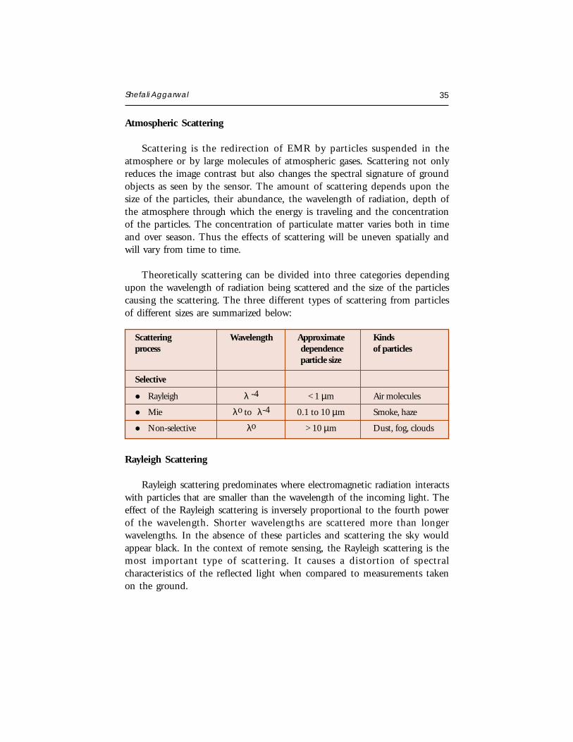
Theoretically scattering can be divided into three categories dependingupon the wavelength of radiation being scattered and the size of the particlescausing the scattering. The three different types of scattering from particlesof different sizes are summarized below:
Scattering Wavelength Approximate Kindsprocess dependence of particles
particle size
Selective
Rayleigh λ -4 < 1 µm Air molecules
Mie λo to λ-4 0.1 to 10 µm Smoke, haze
Non-selective λo > 10 µm Dust, fog, clouds
Rayleigh Scattering
Rayleigh scattering predominates where electromagnetic radiation interactswith particles that are smaller than the wavelength of the incoming light. Theeffect of the Rayleigh scattering is inversely proportional to the fourth powerof the wavelength. Shorter wavelengths are scattered more than longerwavelengths. In the absence of these particles and scattering the sky wouldappear black. In the context of remote sensing, the Rayleigh scattering is themost important type of scattering. It causes a distortion of spectralcharacteristics of the reflected light when compared to measurements takenon the ground.
36 Principles of Remote Sensing
Mie Scattering
Mie scattering occurs when the wavelength of the incoming radiation issimilar in size to the atmospheric particles. These are caused by aerosols: amixture of gases, water vapor and dust. It is generally restricted to the loweratmosphere where the larger particles are abundant and dominates underovercast cloud conditions. It influences the entire spectral region from ultraviolet to near infrared regions.
Non-selective Scattering
This type of scattering occurs when the particle size is much larger thanthe wavelength of the incoming radiation. Particles responsible for this effectare water droplets and larger dust particles. The scattering is independent ofthe wavelength, all the wavelength are scattered equally. The most commonexample of non-selective scattering is the appearance of clouds as white. Ascloud consist of water droplet particles and the wavelengths are scattered inequal amount, the cloud appears as white.
Occurrence of this scattering mechanism gives a clue to the existence oflarge particulate matter in the atmosphere above the scene of interest whichitself is a useful data. Using minus blue filters can eliminate the effects of theRayleigh component of scattering. However, the effect of heavy haze i.e. whenall the wavelengths are scattered uniformly, cannot be eliminated using hazefilters. The effects of haze are less pronounced in the thermal infrared region.Microwave radiation is completely immune to haze and can even penetrateclouds.
Atmospheric Absorption
The gas molecules present in the atmosphere strongly absorb the EMRpassing through the atmosphere in certain spectral bands. Mainly three gasesare responsible for most of absorption of solar radiation, viz. ozone, carbondioxide and water vapour. Ozone absorbs the high energy, short wavelengthportions of the ultraviolet spectrum (λ < 0.24 µm) thereby preventing thetransmission of this radiation to the lower atmosphere. Carbon dioxide isimportant in remote sensing as it effectively absorbs the radiation in mid andfar infrared regions of the spectrum. It strongly absorbs in the region fromabout 13-17.5 µm, whereas two most important regions of water vapourabsorption are in bands 5.5 - 7.0 µm and above 27 µm. Absorption relatively
Shefali Aggarwal 37
reduces the amount of light that reaches our eye making the scene lookrelatively duller.
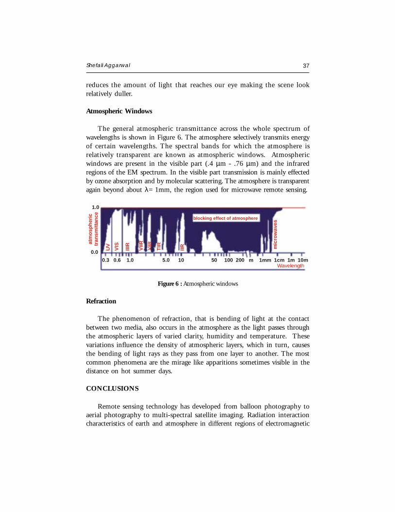
Atmospheric Windows
The general atmospheric transmittance across the whole spectrum ofwavelengths is shown in Figure 6. The atmosphere selectively transmits energyof certain wavelengths. The spectral bands for which the atmosphere isrelatively transparent are known as atmospheric windows. Atmosphericwindows are present in the visible part (.4 µm - .76 µm) and the infraredregions of the EM spectrum. In the visible part transmission is mainly effectedby ozone absorption and by molecular scattering. The atmosphere is transparentagain beyond about λ= 1mm, the region used for microwave remote sensing.
Figure 6 : Atmospheric windows
Refraction
The phenomenon of refraction, that is bending of light at the contactbetween two media, also occurs in the atmosphere as the light passes throughthe atmospheric layers of varied clarity, humidity and temperature. Thesevariations influence the density of atmospheric layers, which in turn, causesthe bending of light rays as they pass from one layer to another. The mostcommon phenomena are the mirage like apparitions sometimes visible in thedistance on hot summer days.
CONCLUSIONS
Remote sensing technology has developed from balloon photography toaerial photography to multi-spectral satellite imaging. Radiation interactioncharacteristics of earth and atmosphere in different regions of electromagnetic
blocking effect of atmosphere
atm
osph
eric
tran
smitt
ance
1.0
0.0
mic
row
aves
0.3 0.6 1.0 5.0 10 50 100 200 m 1mm 1cm 1m 10m Wavelength
UV
VIS
IIIR
VIIR
TIR
IIRVIIR

38 Principles of Remote Sensing
spectrum are very useful for identifying and characterizing earth andatmospheric features.
REFERENCES
Campbell, J.B. 1996. Introduction to Remote Sensing. Taylor & Francis, London.
Colwell, R.N. (Ed.) 1983. Manual of Remote Sensing. Second Edition. Vol I: Theory,Instruments and Techniques. American Society of Photogrammetry and Remote SensingASPRS, Falls Church.
Curran, P.J. 1985. Principles of Remote Sensing. Longman Group Limited, London.
Elachi, C. 1987. Introduction to the Physics and Techniques of Remote Sensing. Wiley Seriesin Remote Sensing, New York.
http://www.ccrs.nrcan.gc.ca/ccrs/learn/tutorials/fundam/chapter1/chapter1_1_e.html
Joseph, G. 1996. Imaging Sensors. Remote Sensing Reviews, 13: 257-342.
Lillesand, T.M. and Kiefer, R.1993. Remote Sensing and Image Interpretation. Third EditionJohn Villey, New York.
Manual of Remote Sensing. IIIrd Edition. American Society of Photogrammtery and RemoteSensing.
Sabins, F.F. 1997. Remote Sensing and Principles and Image Interpretation. WH Freeman,New York.
EARTH RESOURCE SATELLITES
Shefali AggarwalPhotogrammetry and Remote Sensing DivisionIndian Institute of Remote Sensing, Dehra Dun
Abstract : Since the first balloon flight, the possibilities to view the earth’s surfacefrom above had opened up new vistas of opportunities for mankind. The view fromabove has inspired a number of technological developments that offer a wide-rangeof techniques to observe the phenomena on the earth’s surface, under oceans, andunderneath the surface of the earth. While the first imagery used for remote sensingcame from balloons and later from airplanes, today the satellites or spacecraft arewidely used for data collection. The uniqueness of satellite remote sensing lies inits ability to provide a synoptic view of the earth’s surface and to detect features atelectromagnetic wavelengths, which are not visible to the human eye. Data fromsatellite images can show larger areas than aerial survey data and, as a satelliteregularly passes over the same area capturing new data each time, changes in theland use /land cover can be periodically monitored.
In order to use remotely sensed data, the user has to understand the characteristicsof the system being used. The most important system characteristic the user has tounderstand is resolution. Resolution is measured in four ways, spatial, spectral,radiometric and temporal. The article describes the characteristics of satellite orbitsand sensor systems, data capturing mechanisms and then highlights some of the
commercially available satellites and future missions to be undertaken.
INTRODUCTION
Remote sensing is defined as the science which deals with obtaininginformation about objects on earth surface by analysis of data, received
from a remote platform. Since the launch of the first remote sensing weathersatellite (TIROS-1) in 1960 and the first Earth resources satellite in 1972(Landsat-1), various platforms with a variety of remote sensing sensors havebeen launched to study the Earth land cover, the oceans, the atmosphere orto monitor the weather.
Satellite Remote Sensing and GIS Applications in Agricultural Meteorologypp. 39-65
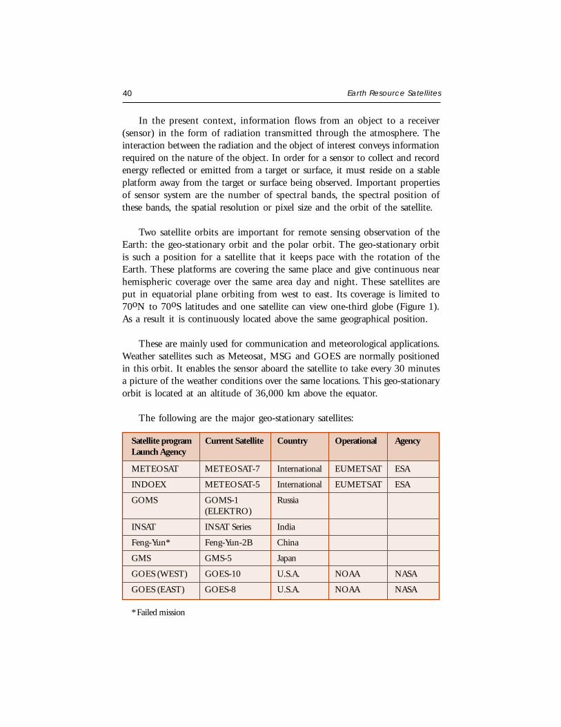
40 Earth Resource Satellites
In the present context, information flows from an object to a receiver(sensor) in the form of radiation transmitted through the atmosphere. Theinteraction between the radiation and the object of interest conveys informationrequired on the nature of the object. In order for a sensor to collect and recordenergy reflected or emitted from a target or surface, it must reside on a stableplatform away from the target or surface being observed. Important propertiesof sensor system are the number of spectral bands, the spectral position ofthese bands, the spatial resolution or pixel size and the orbit of the satellite.
Two satellite orbits are important for remote sensing observation of theEarth: the geo-stationary orbit and the polar orbit. The geo-stationary orbitis such a position for a satellite that it keeps pace with the rotation of theEarth. These platforms are covering the same place and give continuous nearhemispheric coverage over the same area day and night. These satellites areput in equatorial plane orbiting from west to east. Its coverage is limited to70oN to 70oS latitudes and one satellite can view one-third globe (Figure 1).As a result it is continuously located above the same geographical position.
These are mainly used for communication and meteorological applications.Weather satellites such as Meteosat, MSG and GOES are normally positionedin this orbit. It enables the sensor aboard the satellite to take every 30 minutesa picture of the weather conditions over the same locations. This geo-stationaryorbit is located at an altitude of 36,000 km above the equator.
The following are the major geo-stationary satellites:
Satellite program Current Satellite Country Operational AgencyLaunch Agency
METEOSAT METEOSAT-7 International EUMETSAT ESA
INDOEX METEOSAT-5 International EUMETSAT ESA
GOMS GOMS-1 Russia(ELEKTRO)
INSAT INSAT Series India
Feng-Yun* Feng-Yun-2B China
GMS GMS-5 Japan
GOES (WEST) GOES-10 U.S.A. NOAA NASA
GOES (EAST) GOES-8 U.S.A. NOAA NASA
* Failed mission

Shefali Aggarwal 41
The second important remote sensing orbit is the polar orbit. Satellitesin a polar orbit, cycle the Earth from North Pole to South Pole. The polarorbits have an inclination of approximately 99 degrees with the equator tomaintain a sun synchronous overpass i.e. the satellite passes over all places onearth having the same latitude twice in each orbit at the same local sun-time.This ensures similar illumination conditions when acquiring images over aparticular area over a series of days (Figure 2). Image acquisition mostly takesplace in the morning when the sun position is optimal between 9.30 and11.00 hr local time. The altitude of the polar orbits varies from approximately650 to 900 km although spy-satellites are in a much lower orbit.
Figure 2. Near Polar Orbits (source CCRS website)
Figure 1. Geo-stationary Orbit (source CCRS website)
As the satellite orbits the Earth from pole to pole, its east-west positionwould not change if the Earth did not rotate. However, as seen from theEarth, it seems that the satellite is shifting westward because the Earth isrotating (from west to east) beneath it. This apparent movement allows the
Satellite Ground Track
EquatorEarth’s Rotation
Satellite Direction
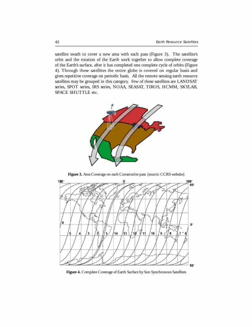
42 Earth Resource Satellites
satellite swath to cover a new area with each pass (Figure 3). The satellite’sorbit and the rotation of the Earth work together to allow complete coverageof the Earth’s surface, after it has completed one complete cycle of orbits (Figure4). Through these satellites the entire globe is covered on regular basis andgives repetitive coverage on periodic basis. All the remote sensing earth resourcesatellites may be grouped in this category. Few of these satellites are LANDSATseries, SPOT series, IRS series, NOAA, SEASAT, TIROS, HCMM, SKYLAB,SPACE SHUTTLE etc.
Figure 3. Area Coverage on each Consecutive pass (source: CCRS website)
Figure 4. Complete Coverage of Earth Surface by Sun Synchronous Satellites
Shefali Aggarwal 43
REMOTE SENSING SENSORS
Sensor is a device that gathers energy (EMR or other), converts it into asignal and presents it in a form suitable for obtaining information about thetarget under investigation. These may be active or passive depending on thesource of energy.
Sensors used for remote sensing can be broadly classified as those operatingin Optical-Infrared (OIR) region and those operating in the microwave region.OIR and microwave sensors can further be subdivided into passive and active.
Active sensors use their own source of energy. Earth surface is illuminatedthrough energy emitted by its own source, a part of it is reflected by the surfacein the direction of the sensor, which is received to gather the information.Passive sensors receive solar electromagnetic energy reflected from the surfaceor energy emitted by the surface itself. These sensors do not have their ownsource of energy and can not be used at nighttime, except thermal sensors.Again, sensors (active or passive) could either be imaging, like camera or sensor,which acquire images of the area and non-imaging types like non-scanningradiometer or atmospheric sounders.
Resolution
Resolution is defined as the ability of the system to render the informationat the smallest discretely separable quantity in terms of distance (spatial),wavelength band of EMR (spectral), time (temporal) and/or radiation quantity(radiometric).
Spatial Resolution
Spatial resolution is the projection of a detector element or a slit onto theground. In other words, scanner’s spatial resolution is the ground segmentsensed at any instant. It is also called ground resolution element (GRE).
The spatial resolution at which data are acquired has two effects – theability to identify various features and quantify their extent. The former onerelates to the classification accuracy and the later to the ability to accuratelymake mensuration. Images where only large features are visible are said to havecoarse or low resolution. In fine resolution images, small objects can be detected.
44 Earth Resource Satellites
Spectral Resolution
Spectral emissivity curves characterize the reflectance and/or emittance ofa feature or target over a variety of wavelengths. Different classes of featuresand details in an image can be distinguished by comparing their responsesover distinct wavelength ranges. Broad classes such as water and vegetationcan be separated using broad wavelength ranges (VIS, NIR), whereas specificclasses like rock types would require a comparison of fine wavelength rangesto separate them. Hence spectral resolution describes the ability of the sensorto define fine wavelength intervals i.e. sampling the spatially segmented imagein different spectral intervals, thereby allowing the spectral irradiance of theimage to be determined.
Radiometric Resolution
This is a measure of the sensor to differentiate the smallest change in thespectral reflectance/emittance between various targets. The radiometricresolution depends on the saturation radiance and the number of quantisationlevels. Thus, a sensor whose saturation is set at 100% reflectance with an 8bit resolution will have a poor radiometric sensitivity compared to a sensorwhose saturation radiance is set at 20% reflectance and 7 bit digitization.
Temporal Resolution
Obtaining spatial and spectral data at certain time intervals. Temporalresolution is also called as the repetivity of the satellite; it is the capability ofthe satellite to image the exact same area at the same viewing angle at differentperiods of time. The temporal resolution of a sensor depends on a variety offactors, including the satellite/sensor capabilities, the swath overlap andlatitude.
Multispectral Scanning Principle
Cameras and their use for aerial photography are the simplest and oldestof sensors used for remote sensing of the Earth’s surface. Cameras are framingsystems (Figure 5a), which acquire a near-instantaneous “snapshot” of an areaof the Earth’s surface. Camera systems are passive optical sensors that use alens (or system of lenses collectively referred to as the optics) to form an imageat the focal plane, the “aerial image plane” at which an image is sharplydefined.
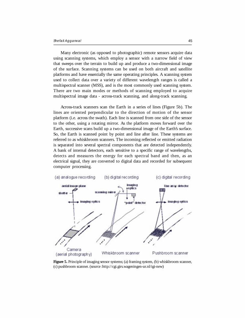
Shefali Aggarwal 45
Many electronic (as opposed to photographic) remote sensors acquire datausing scanning systems, which employ a sensor with a narrow field of viewthat sweeps over the terrain to build up and produce a two-dimensional imageof the surface. Scanning systems can be used on both aircraft and satelliteplatforms and have essentially the same operating principles. A scanning systemused to collect data over a variety of different wavelength ranges is called amultispectral scanner (MSS), and is the most commonly used scanning system.There are two main modes or methods of scanning employed to acquiremultispectral image data - across-track scanning, and along-track scanning.
Across-track scanners scan the Earth in a series of lines (Figure 5b). Thelines are oriented perpendicular to the direction of motion of the sensorplatform (i.e. across the swath). Each line is scanned from one side of the sensorto the other, using a rotating mirror. As the platform moves forward over theEarth, successive scans build up a two-dimensional image of the Earth’s surface.So, the Earth is scanned point by point and line after line. These systems arereferred to as whiskbroom scanners. The incoming reflected or emitted radiationis separated into several spectral components that are detected independently.A bank of internal detectors, each sensitive to a specific range of wavelengths,detects and measures the energy for each spectral band and then, as anelectrical signal, they are converted to digital data and recorded for subsequentcomputer processing.
Figure 5. Principle of imaging sensor systems; (a) framing system, (b) whiskbroom scanner,(c) pushbroom scanner. (source :http://cgi.girs.wageningen-ur.nl/igi-new)
46 Earth Resource Satellites
Along-track scanners also use the forward motion of the platform to recordsuccessive scan lines and build up a two-dimensional image, perpendicular tothe flight direction (Figure 5c). However, instead of a scanning mirror, theyuse a linear array of detectors (so-called charge-coupled devices, CCDs) locatedat the focal plane of the image formed by lens systems, which are “pushed”along in the flight track direction (i.e. along track). These systems are alsoreferred to as push broom scanners, as the motion of the detector array isanalogous to a broom being pushed along a floor. A separate linear array isrequired to measure each spectral band or channel. For each scan line, theenergy detected by each detector of each linear array is sampled electronicallyand digitally recorded.
Regardless of whether the scanning system used is either of these two types,it has several advantages over photographic systems. The spectral range ofphotographic systems is restricted to the visible and near-infrared regions whileMSS systems can extend this range into the thermal infrared. They are alsocapable of much higher spectral resolution than photographic systems. Multi-band or multispectral photographic systems use separate lens systems toacquire each spectral band. This may cause problems in ensuring that thedifferent bands are comparable both spatially and radiometrically and withregistration of the multiple images. MSS systems acquire all spectral bandssimultaneously through the same optical system to alleviate these problems.Photographic systems record the energy detected by means of a photochemicalprocess which is difficult to measure and to make consistent. Because MSSdata are recorded electronically, it is easier to determine the specific amountof energy measured, and they can record over a greater range of values in adigital format. Photographic systems require a continuous supply of film andprocessing on the ground after the photos have been taken. The digitalrecording in MSS systems facilitates transmission of data to receiving stationson the ground and immediate processing of data in a computer environment.
Thermal Scanner
Many multispectral (MSS) systems sense radiation in the thermal infraredas well as the visible and reflected infrared portions of the spectrum. However,remote sensing of energy emitted from the Earth’s surface in the thermalinfrared (3 µm to 15 µm) is different from the sensing of reflected energy.Thermal sensors use photo detectors sensitive to the direct contact of photonson their surface, to detect emitted thermal radiation. The detectors are cooledto temperatures close to absolute zero in order to limit their own thermal
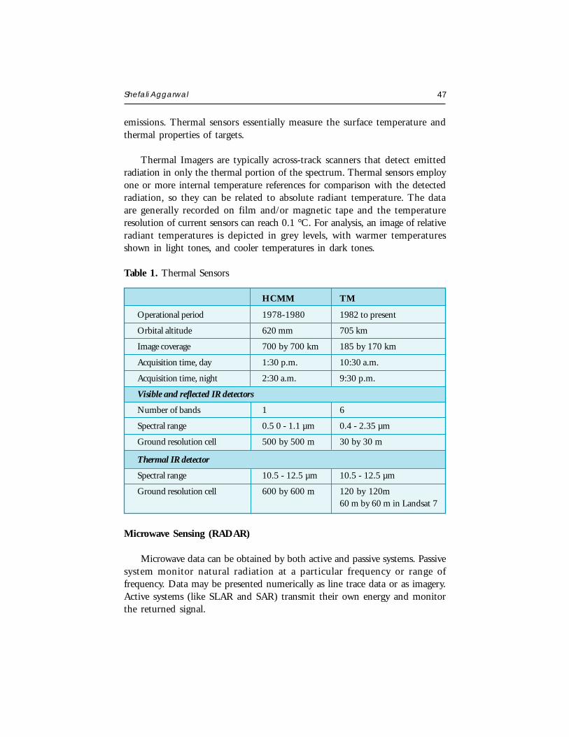
Shefali Aggarwal 47
emissions. Thermal sensors essentially measure the surface temperature andthermal properties of targets.
Thermal Imagers are typically across-track scanners that detect emittedradiation in only the thermal portion of the spectrum. Thermal sensors employone or more internal temperature references for comparison with the detectedradiation, so they can be related to absolute radiant temperature. The dataare generally recorded on film and/or magnetic tape and the temperatureresolution of current sensors can reach 0.1 °C. For analysis, an image of relativeradiant temperatures is depicted in grey levels, with warmer temperaturesshown in light tones, and cooler temperatures in dark tones.
Table 1. Thermal Sensors
HCMM TM
Operational period 1978-1980 1982 to present
Orbital altitude 620 mm 705 km
Image coverage 700 by 700 km 185 by 170 km
Acquisition time, day 1:30 p.m. 10:30 a.m.
Acquisition time, night 2:30 a.m. 9:30 p.m.
Visible and reflected IR detectors
Number of bands 1 6
Spectral range 0.5 0 - 1.1 µm 0.4 - 2.35 µm
Ground resolution cell 500 by 500 m 30 by 30 m
Thermal IR detector
Spectral range 10.5 - 12.5 µm 10.5 - 12.5 µm
Ground resolution cell 600 by 600 m 120 by 120m60 m by 60 m in Landsat 7
Microwave Sensing (RADAR)
Microwave data can be obtained by both active and passive systems. Passivesystem monitor natural radiation at a particular frequency or range offrequency. Data may be presented numerically as line trace data or as imagery.Active systems (like SLAR and SAR) transmit their own energy and monitorthe returned signal.
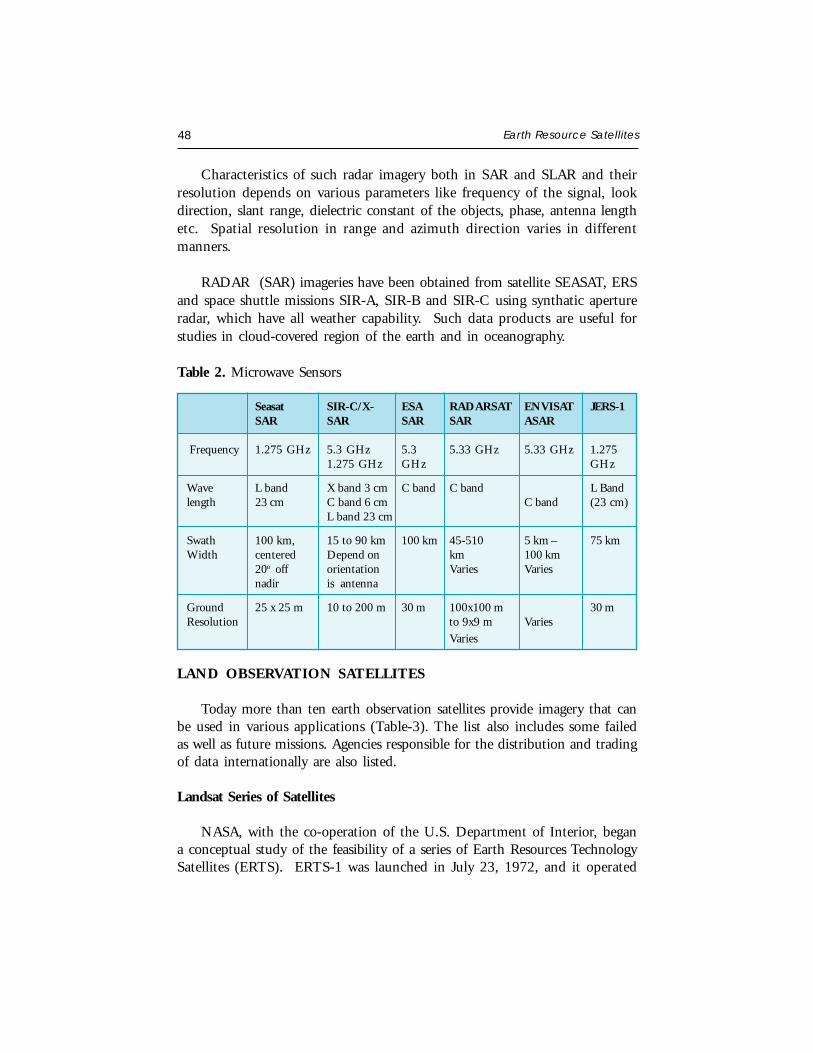
48 Earth Resource Satellites
Characteristics of such radar imagery both in SAR and SLAR and theirresolution depends on various parameters like frequency of the signal, lookdirection, slant range, dielectric constant of the objects, phase, antenna lengthetc. Spatial resolution in range and azimuth direction varies in differentmanners.
RADAR (SAR) imageries have been obtained from satellite SEASAT, ERSand space shuttle missions SIR-A, SIR-B and SIR-C using synthatic apertureradar, which have all weather capability. Such data products are useful forstudies in cloud-covered region of the earth and in oceanography.
Table 2. Microwave Sensors
Seasat SIR-C/X- ESA RADARSAT ENVISAT JERS-1SAR SAR SAR SAR ASAR
Frequency 1.275 GHz 5.3 GHz 5.3 5.33 GHz 5.33 GHz 1.2751.275 GHz GHz GHz
Wave L band X band 3 cm C band C band L Bandlength 23 cm C band 6 cm C band (23 cm)
L band 23 cm
Swath 100 km, 15 to 90 km 100 km 45-510 5 km – 75 kmWidth centered Depend on km 100 km
20o off orientation Varies Variesnadir is antenna
Ground 25 x 25 m 10 to 200 m 30 m 100x100 m 30 mResolution to 9x9 m Varies
Varies
LAND OBSERVATION SATELLITES
Today more than ten earth observation satellites provide imagery that canbe used in various applications (Table-3). The list also includes some failedas well as future missions. Agencies responsible for the distribution and tradingof data internationally are also listed.
Landsat Series of Satellites
NASA, with the co-operation of the U.S. Department of Interior, begana conceptual study of the feasibility of a series of Earth Resources TechnologySatellites (ERTS). ERTS-1 was launched in July 23, 1972, and it operated
Shefali Aggarwal 49
until January 6, 1978. It represented the first unmanned satellite specificallydesigned to acquire data about earth resources on a systematic, repetitive,medium resolution, multispectral basis. It was primarily designed as anexperimental system to test the feasibility of collecting earth resources datafrom unmanned satellites. About 300 individual ERTS-1 experiments wereconducted in 43 US states and 36 nations. Just prior to the launch of ERTS-B on January 22nd 1975, NASA officially renamed the ERTS programme asthe “LANDSAT” programme. All subsequent satellites in the series carriedthe Landsat designation. So far six Landsat satellites have been launchedsuccessfully, while Landsat-6 suffered launch failure. Table-4 highlights thecharacteristics of the Landsat series satellites. There have been four differenttypes of sensors included in various combinations on these missions. Theseare Return Beam Vidicon camera (RBV) systems, Multispectral Scanner (MSS)systems, Thematic Mapper (TM) and Enhanced Thematic Mapper (ETM).
After more than two decades of success, the Landsat program realised itsfirst unsuccessful mission with the launch failure of Landsat-6 on October 5,1993. The sensor included on-board was the Enhanced Thematic Mapper(ETM). To provide continuity with Landsat -4 and -5 the ETM incorporatedthe same seven spectral bands and the same spatial resolutions as the TM.The ETM’s major improvement over the TM was addition of an eighthpanchromatic band operating in 0.50 to 0.90-µm range and spatial resolutionof 15m. Landsat-7 includes two sensors: the Enhanced Thematic Mapper plus(ETM+) and the High Resolution Multispectral Stereo Imager (HRMSI).
Spot Series of Satellite
French Government in joint programme with Sweden and Belgiumundertook the development of Systeme Pour l’Observation de la Terre (SPOT)program. Conceived and designed by the French Center National d’EtudesSpatiales (CNES), SPOT has developed into a large-scale internationalprogramme with ground receiving stations and data distribution outlets locatedin more than 30 countries. It is also the first system to have pointable optics.This enables side-to-side off-nadir viewing capabilities, and it affords full scenestereoscopic imaging from two different satellite tracks permitting coverageof the same area. SPOT-1 was retired from full-time services on December31, 1990. The SPOT-2 satellite was launched on January 21, 1990, andSPOT-3 was launched on September 25, 1993. SPOT-4 was launched on26 March, 1998. Characteristics of SPOT Satellites are presented in Table 5.

50 Earth Resource Satellites
Tab
le 3
. O
pera
tion
al E
arth
Obs
erva
tion
Sat
ellit
es
EU
RO
PE
MID
DLE
N
OR
TH
AM
ER
ICA
ASI
AE
AST
Fran
ceE
SAIs
rael
U
SAC
anad
aIn
dia
Japa
n
SPO
T1-
1986
LAN
DSA
T5
10m
-85,
30m
SPO
T2-
90E
RS1
-92/
00LA
ND
SAT
6-10
m R
adar
93
SPO
T3-
93/9
6E
RS2
-95
EAR
LYB
IRD
IKO
NO
S1-
RA
DA
RSA
T-IR
S1C
-95
Rad
ar-9
899
, 1m
95 6
m
SPO
T4-
98E
NV
ISAT
-LA
ND
SAT
7-IK
ON
OS2
IRS1
D-9
710
m20
01R
adar
99, 1
5m-9
9, 1
m 6
m
ERO
S A
/Q
UIC
KB
IRD
-O
RBV
IEW
-1-
00 2
m01
, 0.6
m01
, 1m
SPO
T5-
02ER
OS
B/
OR
BV
IEW
RA
DA
RSA
TIR
S-P6
-03,
ALO
S-3m
+ H
RS1
01-
02, 1
m-0
2, 1
m-0
36M
MSS
03, 2
.5m
Dis
trib
utio
n
SPO
TM
iscel
lane
ous
Imag
esat
SI-E
OSA
T, E
arth
wat
ch,
RA
DA
RSA
TN
RSA
-JS
IIM
AG
ING
Orb
imag
e, U
SGS
EO
SAT
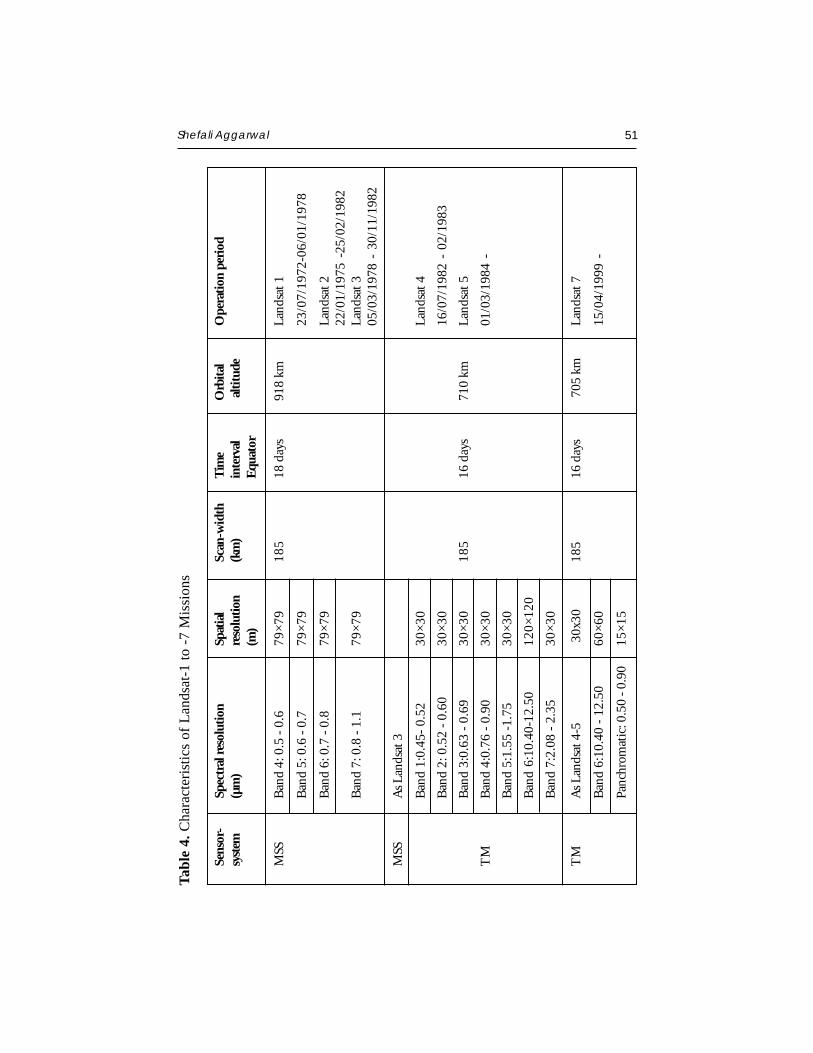
Shefali Aggarwal 51
Tabl
e 4.
Cha
ract
eris
tics
of L
ands
at-1
to -7
Mis
sion
s
Sens
or-
Spec
tral
reso
lutio
nSp
atia
lSc
an-w
idth
Tim
eO
rbita
lO
pera
tion
peri
odsy
stem
(µm
)re
solu
tion
(km
)in
terv
al a
ltitu
de(m
)E
quat
or
MSS
Ban
d 4:
0.5
- 0.
679
×79
185
18 d
ays
918
kmLa
ndsa
t 1
Ban
d 5:
0.6
- 0.
779
×79
23/0
7/19
72-0
6/01
/197
8
Ban
d 6:
0.7
- 0.
879
×79
Land
sat 2
22/0
1/19
75 -
25/0
2/19
82B
and
7: 0
.8 -
1.1
79×7
9La
ndsa
t 305
/03/
1978
- 3
0/11
/198
2
MSS
As L
ands
at 3
Ban
d 1:
0.45
- 0.
5230
×30
Land
sat 4
Ban
d 2:
0.5
2 -
0.60
30×3
016
/07/
1982
- 0
2/19
83
Ban
d 3:
0.63
- 0
.69
30×3
018
516
day
s71
0 km
Land
sat 5
TM
Ban
d 4:
0.76
- 0
.90
30×3
001
/03/
1984
-
Ban
d 5:
1.55
-1.
7530
×30
Ban
d 6:
10.4
0-12
.50
120×
120
Ban
d 7:
2.08
- 2
.35
30×3
0
TM
As L
ands
at 4
-5 3
0x30
185
16 d
ays
705
km
Land
sat 7
Ban
d 6:
10.4
0 -
12.5
060
×60
15/0
4/19
99 -
Panc
hrom
atic
: 0.5
0 - 0
.90
15×1
5
52 Earth Resource Satellites
SPOT-4 includes the additional 20m-resolution band in the mid-infraredportion of the spectrum (between 1.58 and 1.75 µm). This band is intendedto improve vegetation monitoring and mineral discriminating capabilities ofthe data. Furthermore, mixed 20m and 10m data sets will be co-registeredon-board instead of during ground processing. This will be accomplished byreplacing the panchromatic band of SPOT-1, -2 and -3 (0.49 to 0.73 µm)with red band from these systems (0.61 to 0.68 µm). This band will be usedto produce both 10m black and white images and 20m multispectral data.Another change in SPOT-4 is the addition of a separate wide-field-of-view,sensor called the Vegetation Monitoring Instrument (VMI).
IRS Satellite Series
The Indian Space programme has the goal of harnessing space technologyfor application in the areas of communications, broadcasting, meteorology andremote sensing. The important milestones crossed so far are Bhaskara-1 and2 (1979) the experimental satellites, which carried TV Cameras and MicrowaveRadiometers. The Indian Remote Sensing (IRS) Satellite was the next logicalstep towards the National operational satellites, which directly generatesresources information in a variety of application areas such as forestry, geology,agriculture and hydrology. IRS -1A/1B, carried Linear Imaging Self Scanningsensors LISS-I & LISS-II (Table 6). IRS-P2 was launched in October 1994on PSLV-D2, an indigenous launch vehicle. IRS-1C, was launched onDecember 28, 1995, which carried improved sensors like LISS-III, WiFS, PANCamera, etc. Details of IRS series platforms are given in the following section.IRS-P3 was launched into the sun synchronous orbit by another indigenouslaunch vehicle PSLV - D3 on 21.3.1996 from Indian launching stationSriharikota (SHAR). IRS-1D was launched on 29 September 1997 and IRS-P4 was launched on 26 – 5-1999 on-board PSLV from Sriharikota.
IRS-P4 carrying an Ocean Colour Monitor (OCM) and a Multi-frequencyScanning Microwave Radiometer (MSMR) was launched on May 26, 1999.OCM has 8 narrow spectral bands operating in visible and near-infrared bands(402-885 nm) with a spatial resolution of 360 m and swath of 1420 km.IRS-P4 OCM thus provides highest spatial resolution compared to any othercontemporary satellites in the international arena during this time frame. TheMSMR with its all weather capability is configured to have measurements at4 frequencies (6.6, 10.6, 18 & 26 GHZ) with an overall swath of 1360 km.The spatial resolution is 120, 80, 40 and 40 km for the frequency bands of
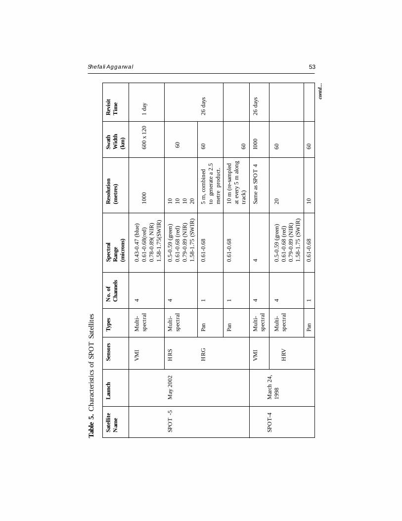
Shefali Aggarwal 53
Tab
le 5
. C
hara
cter
isti
cs o
f SP
OT
Sat
ellit
es
Sate
llite
Laun
chSe
nsor
sTy
pes
No.
of
Spec
tral
Res
olut
ion
Swat
hR
evis
itN
ame
Cha
nnel
sR
ange
(met
res)
Wid
thT
ime
(mic
rons
)(k
m)
VM
IM
ulti
-4
0.43
-0.4
7 (b
lue)
spec
tral
0.61
-0.6
8(re
d)10
0060
0 x
120
1 da
y0.
78-0
.89(
NIR
)1.
58-1
.75(
SWIR
)
SPO
T -
5M
ay 2
002
HR
SM
ulti
-4
0.5-
0.59
(gr
een)
10sp
ectr
al0.
61-0
.68
(red
)10
60
0.79
-0.8
9 (N
IR)
101.
58-1
.75
(SW
IR)
20
HR
GPa
n1
0.61
-0.6
85
m, c
ombi
ned
6026
day
sto
ge
nera
te a
2.5
met
re p
rodu
ct.
Pan
10.
61-0
.68
10 m
(re
-sam
pled
at e
very
5 m
alo
ngtr
ack)
60
VM
IM
ulti
-4
4Sa
me
as S
POT
4I0
0026
day
ssp
ectr
alSP
OT
-4M
arch
24,
1998
Mul
ti-
40.
5-0.
59 (
gree
n)20
60H
RV
spec
tral
0.61
-0.6
8 (r
ed)
0.79
-0.8
9 (N
IR)
1.58
-1.7
5 (S
WIR
)
Pan
10.
61-0
.68
1060
cont
d...
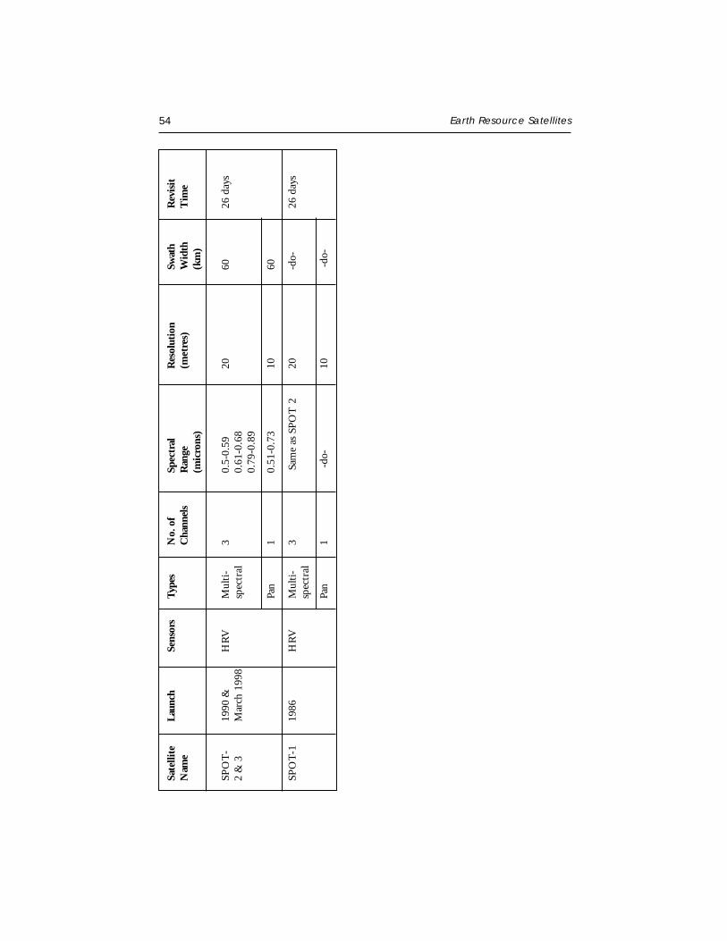
54 Earth Resource Satellites
SPO
T-
1990
&H
RV
Mul
ti-
30.
5-0.
5920
6026
day
s2
& 3
Mar
ch 1
998
spec
tral
0.61
-0.6
80.
79-0
.89
Pan
10.
51-0
.73
1060
SPO
T-1
1986
HR
VM
ulti
-3
Sam
e as
SPO
T 2
20-d
o-
26 d
ays
spec
tral
Pan
1 -
do-
10 -
do-
Sate
llite
Laun
chSe
nsor
sTy
pes
No.
of
Spec
tral
Res
olut
ion
Swat
hR
evis
itN
ame
Cha
nnel
sR
ange
(met
res)
Wid
thT
ime
(mic
rons
)(k
m)
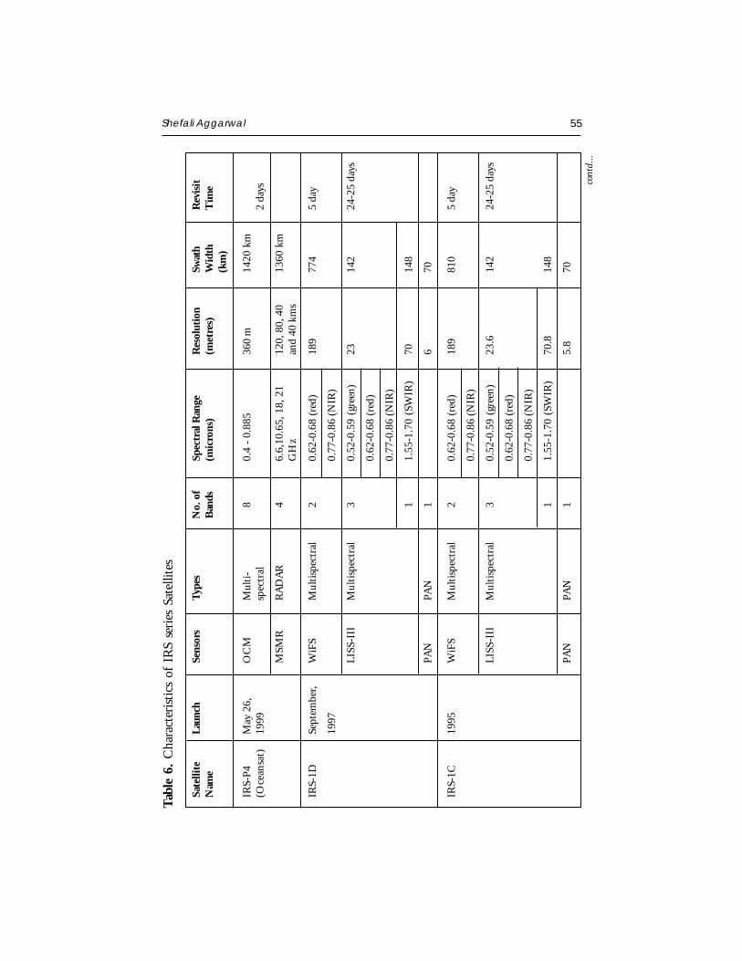
Shefali Aggarwal 55
Tab
le 6
. C
hara
cter
isti
cs o
f IR
S se
ries
Sat
ellit
es
Sate
llite
Laun
chSe
nsor
sTy
pes
No.
of
Spec
tral
Ran
geR
esol
utio
nSw
ath
Rev
isit
Nam
eB
ands
(mic
rons
)(m
etre
s)W
idth
Tim
e(k
m)
IRS-
P4
May
26,
OC
MM
ulti
-8
0.4
- 0.
885
360
m14
20 k
m(O
cean
sat)
1999
spec
tral
2 da
ys
MSM
RR
AD
AR
46.
6,10
.65,
18,
21
120,
80,
40
13
60 k
mG
Hz
and
40 k
ms
IRS-
1DSe
ptem
ber,
WiF
SM
ulti
spec
tral
20.
62-0
.68
(red
)18
977
45
day
1997
0.77
-0.8
6 (N
IR)
LIS
S-II
IM
ulti
spec
tral
30.
52-0
.59
(gre
en)
2314
224
-25
days
0.62
-0.6
8 (r
ed)
0.77
-0.8
6 (N
IR)
11.
55-1
.70
(SW
IR)
7014
8
PAN
PAN
1
670
IRS-
1C19
95W
iFS
Mul
tisp
ectr
al2
0.62
-0.6
8 (r
ed)
189
810
5 da
y
0.77
-0.8
6 (N
IR)
LIS
S-II
IM
ulti
spec
tral
30.
52-0
.59
(gre
en)
23.6
142
24-2
5 da
ys
0.62
-0.6
8 (r
ed)
0.77
-0.8
6 (N
IR)
11.
55-1
.70
(SW
IR)
70.8
148
PAN
PAN
1
5.8
70
cont
d...

56 Earth Resource Satellites
Sate
llite
Laun
chSe
nsor
sTy
pes
No.
of
Spec
tral
Ran
geR
esol
utio
nSw
ath
Rev
isit
Nam
eB
ands
(mic
rons
)(m
etre
s)W
idth
Tim
e(k
m)
IRS-
1B19
91L
ISS-
IM
ulti
spec
tral
445
0-52
072
.514
822
day
s
0.52
-0.5
9
0.62
-0.6
8
0.77
-0.8
6 (N
IR)
LIS
S-II
Mul
tisp
ectr
al4
(sam
e as
LIS
S I)
36.2
574
IRS-
1A19
88L
ISS-
IM
ulti
spec
tral
4Sa
me
as a
bove
72.5
148
LIS
S-II
Mul
tisp
ectr
al4
Sam
e as
abo
ve36
.25
74
22 d
ays
Shefali Aggarwal 57
6.6., 10.6, 18 and 21 GHz. MSMR will also be in a way a unique sensor asno other passive microwave radiometer is operational in the civilian domaintoday and will be useful for study of both physical oceanographic andmeteorological parameters.
FUTURE INDIAN SATELLITE MISSIONS
Encouraged by the successful operation of the present IRS missions, manymore missions have been planned for realization in the next few years. Thesemissions will have suitable sensors for applications in cartography, crop andvegetation monitoring, oceanography and atmospheric studies.
CARTOSAT-1:
It will have a cutting-edge technology in terms of sensor systems and willprovide state-of-art capabilities for cartographic applications. The satellitewill have only a PAN camera with 2.5 m resolution and 30 km swath andFore-Aft stereo capability. The 2.5 m resolution data will cater to the specificneeds of cartography and terrain modeling applications.
RESOURCESAT-1:
Launched on 17th October, 2003, it is designed mainly for resourcesapplications and having 3-band multi-spectral LISS-4 camera with a spatialresolution 5.8m and a swath of around 24 km with across – track steerabilityfor selected area monitoring. An improved version of LISS-III, with 4 bands(green, red, near—IR and SWIR), all at 23.5 meters resolution and 140 kmswath will also provide the much essential continuity to LISS-III. Thesepayloads will provide enhanced data for vegetation applications and will allowmultiple crop discrimination; species level discrimination and so on. Togetherwith an advanced wide-field sensor, WiFS with ~ 60 m resolution and ~ 740km swath, the payloads will aid greatly for crop and vegetation applicationsand integrated land and water applications. The data will also be useful forhigh accuracy resources management applications, where the emphasis is onmulti crop mapping studies, vegetation species identification and utilitiesmapping.
CLIMATSAT/OCEANSAT-2:
In order to meet the information requirements to study the Planet Earthas an integrated system, satellite missions are planned which would enable
58 Earth Resource Satellites
global observations of climate, ocean and the atmosphere, particularly coveringthe tropical regions, where sufficient data sets are not available. Theinstruments like radiometers, sounders, spectrometers etc. for studying theland, ocean and atmospheric interactions are being planned for these missions.
OTHER COMMERCIALLY AVAILABLE SATELLITES
IKONOS:
The IKONOS-2 satellite was launched in September 1999 and has beendelivering commercial data since early 2000. IKONOS is the first of the nextgeneration of high spatial resolution satellites. IKONOS data records 4channels of multispectral data at 4 m resolution and one panchromatic channelwith 1 m resolution (Table 7). This means that IKONOS is first commercialsatellite to deliver near photographic quality imagery of anywhere in the worldfrom space. Radiometric Resolution: Data is collected as 11 bits per pixel(2048 gray tones).
The applications for this data are boundless: in particular, it will be usedfor large scale mapping, creating precise height models for e.g. micro-cellularradio, and for every application requiring the utmost detail from areas whichare inaccessible for aerial photography.
ENVISAT:
Envisat launched on 1st March 2002 is the most powerful European Earth-observation satellite. Envisat is a key element of the European Space Agency’splans for the next decade to monitor Earth’s environment. It carries instrumentsto collect information that will help scientists to understand each part of theEarth system and to predict how changes in one part will affect others (Table8). It is in a Sun synchronous orbit at an altitude of 800 km and carrying10 instruments onboard.
Variety of earth resources satellites are currently commercially availablefor inventorying and monitoring earth resources. These satellites arecharacterised by varying spatial, spectral, radiometric and temporal resolutions(Table 9).

Shefali Aggarwal 59
Tab
le 7
. C
hara
cter
isti
c of
IK
ON
OS
Sate
llite
Sate
llite
Laun
chSe
nsor
sTy
pes
No.
of
Spec
tral
Ran
geR
esol
utio
nSw
ath
Rev
isit
Nam
eB
ands
(mic
rons
)(m
etre
s)W
idth
Tim
e(k
m)
IKO
NO
S-2
Sept
embe
rIK
ON
OS
Mul
ti-s
pect
ral
40.
45-0
.52
(blu
e)4
11
day
s
24, 1
999
0.52
-0.6
0 (g
reen
)
0.63
-0.6
9 (r
ed)
0.76
-0.9
0 (N
IR)
PAN
1
1
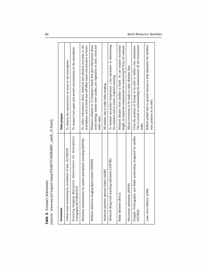
60 Earth Resource Satellites
Tab
le 8
. E
nvis
at’s
Inst
rum
ent
(sou
rce:
ww
w.e
sa.in
t/ex
port
/esa
sa/E
SAD
TO
MB
AM
C_e
arth
_O.h
tml)
Inst
rum
ent
Glo
bal o
zone
mon
itor
ing
by o
ccul
tati
on o
f st
ars
(G
OM
OS)
Scan
nin
g Im
agin
g A
bso
rpti
on S
pec
trom
eter
for
Atm
osp
her
icC
arto
grap
hy (S
CIA
MA
CH
Y)
Mic
hels
on in
terf
erom
eter
for
pas
sive
atm
osph
eric
sou
ndin
g (M
IPA
S)
Med
ium
res
olut
ion
imag
ing
Spec
trom
eter
(M
ER
IS)
Adv
ance
d sy
nthe
tic
aper
ture
Rad
ar (
ASA
R)
Adv
ance
d al
ong
trac
k sc
anni
ng r
adio
met
er (
AA
TSR
)
Rad
ar A
ltim
eter
(R
A-2
)
Mic
row
ave
radi
omet
er (
MW
R)
Dop
pler
Orb
itog
raph
y an
d R
adio
pos
itio
ning
int
egra
ted
by s
atel
lite
(DO
RIS
)
Las
er r
etro
-ref
lect
or (
LR
R)
Mai
n pu
rpos
e
To o
bser
ve t
he c
once
ntra
tion
of
ozon
e in
the
str
atos
pher
e.
To m
easu
re t
race
gas
es a
nd a
eros
ol c
once
ntra
tion
s in
the
atm
osph
ere.
To c
olle
ct i
nfor
mat
ion
abou
t ch
emic
al a
nd p
hysi
cal
proc
esse
s in
the
stra
tosp
here
, suc
h as
thos
e th
at w
ill a
ffec
t ozo
ne c
once
ntra
tion
in fu
ture
.
Mea
sure
s ra
diat
ion
in 1
5 fr
eque
ncy
band
s th
at g
ive
info
rmat
ion
abou
toc
ean
biol
ogy,
mar
ine
wat
er q
ualit
y, a
nd v
eget
atio
n on
land
, clo
ud a
ndw
ater
vap
or.
All
wea
ther
, day
or
nigh
t rad
ar im
agin
g.
To m
easu
re s
ea-s
urfa
ce t
empe
ratu
re,
a ke
y pa
ram
eter
in
dete
rmin
ing
the
exis
tenc
e an
d/or
ext
ent
of g
loba
l war
min
g.
Mea
sure
s di
stan
ce f
rom
sat
ellit
e to
Ear
th.
So c
an m
easu
re s
ea-s
urfa
cehe
ight
, an
impo
rtan
t mea
sure
men
t for
mon
itor
ing
El N
ino,
for
exam
ple.
Allo
ws
corr
ecti
ons
to b
e m
ade
to r
adar
alt
imet
er d
ata.
Giv
es t
he p
osit
ion
of E
nvis
at i
n it
s or
bit
to w
ithi
n a
few
cen
tim
eter
s.T
his
is c
ruci
al t
o un
ders
tand
ing
the
mea
sure
men
ts a
ll th
e in
stru
men
tsm
ake.
Ref
lect
s pu
lsed
lase
r to
gro
und
stat
ions
to
help
det
erm
ine
the
sate
llite
’sex
act
posi
tion
in
its
orbi
t.

Shefali Aggarwal 61
Tab
le 9
. C
hara
cter
isti
cs o
f so
me
mor
e co
mm
erci
ally
ava
ilabl
e sa
telli
tes
Sate
llite
Laun
chSe
nsor
sTy
pes
No.
of
Spec
tral
Ran
geR
esol
utio
nSw
ath
Rev
isit
Nam
eB
ands
(mic
rons
)(m
etre
s)W
idth
Tim
e(k
m)
Qui
ckB
ird-
2O
ct. 1
8, 2
001
M
ulti
-4
blue
(0.
45-0
.52)
2.5
17
spec
tral
gree
n (0
.52-
0.6)
red
(0.6
3-0.
69)
NIR
.(76
-0.8
9)
Pan
10.
45-0
.90.
61
ER
OS
1D
ec. 5
, 200
0
Pan
10.
5-0.
91.
812
.51-
4 da
ys
EO
1N
ov. 2
1, 2
000
ALI
Mul
ti9
0.43
3-0.
453
0.45
-0.5
15
0.52
5-0.
605
0.63
-0.6
9
0.77
5-0.
805
0.84
5-0.
89
1.2-
1.3
1.55
-1.7
5
2.08
-2.3
530
3716
day
s
Pan
10.
48-0
.69
10
Hyp
erio
nH
yper
220
0.4
to 2
.5 (
10nm
307.
5 km
xsa
mpl
ing
inte
rval
)10
0 km
cont
d...
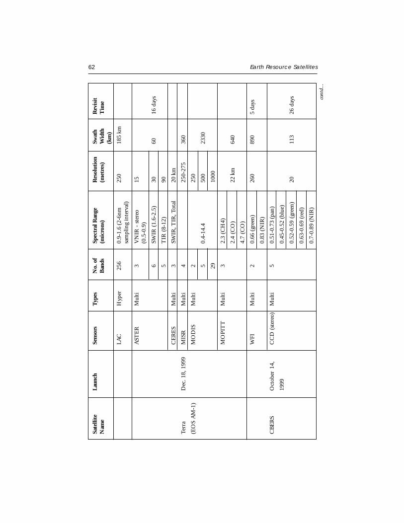
62 Earth Resource Satellites
LAC
Hyp
er25
60.
9-1.
6 (2
-6nm
250
185
kmsa
mpl
ing
inte
rval
)
AST
ER
Mul
ti3
VN
IR -
ste
reo
15(0
.5-0
.9)
6SW
IR (
1.6-
2.5)
3060
16 d
ays
5T
IR (
8-12
)90
CE
RE
SM
ulti
3SW
IR, T
IR, T
otal
20 k
m
Terr
aD
ec. 1
8, 1
999
MIS
RM
ulti
4
250-
275
360
(EO
S A
M-1
)M
OD
ISM
ulti
225
0
50.
4-14
.450
023
30
2910
00
MO
PIT
TM
ulti
32.
3 (C
H4)
2.4
(CO
)22
km
640
4.7
(CO
)
WFI
Mul
ti2
0.66
(gr
een)
260
890
5 da
ys
0.83
(N
IR)
CB
ER
SO
ctob
er 1
4,C
CD
(st
ereo
)M
ulti
50.
51-0
.73
(pan
)
1999
0.45
-0.5
2 (b
lue)
0.52
-0.5
9 (g
reen
)20
113
26 d
ays
0.63
-0.6
9 (r
ed)
0.7-
0.89
(N
IR)
Sate
llite
Laun
chSe
nsor
sTy
pes
No.
of
Spec
tral
Ran
geR
esol
utio
nSw
ath
Rev
isit
Nam
eB
ands
(mic
rons
)(m
etre
s)W
idth
Tim
e(k
m)
cont
d...
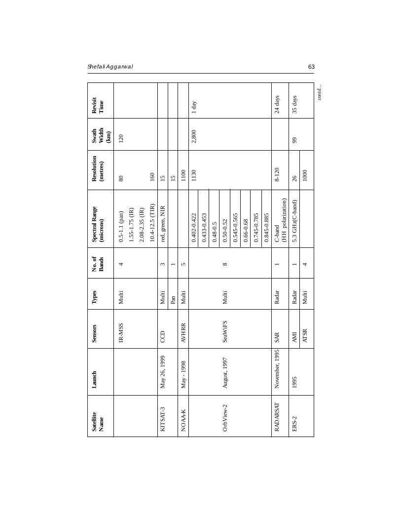
Shefali Aggarwal 63
IR-M
SSM
ulti
40.
5-1.
1 (p
an)
8012
0
1.55
-1.7
5 (I
R)
2.08
-2.3
5 (I
R)
10.4
-12.
5 (T
IR)
160
KIT
SAT
-3M
ay 2
6, 1
999
CC
DM
ulti
3re
d, g
reen
, NIR
15
Pan
1
15
NO
AA
-KM
ay -
199
8AV
HR
RM
ulti
5
1100
0.40
2-0.
422
1130
2,80
01
day
0.43
3-0.
453
0.48
-0.5
Orb
Vie
w-2
Aug
ust,
199
7Se
aWiF
SM
ulti
80.
50-0
.52
0.54
5-0.
565
0.66
-0.6
8
0.74
5-0.
785
0.84
5-0.
885
RA
DA
RSA
TN
ovem
ber,
1995
SAR
Rad
ar1
C-b
and
8-12
0
24 d
ays
(HH
pol
ariz
atio
n)
ER
S-2
1995
AM
IR
adar
15.
3 G
Hz(
C-b
and)
2699
35 d
ays
ATSR
Mul
ti4
10
00
Sate
llite
Laun
chSe
nsor
sTy
pes
No.
of
Spec
tral
Ran
geR
esol
utio
nSw
ath
Rev
isit
Nam
eB
ands
(mic
rons
)(m
etre
s)W
idth
Tim
e(k
m)
cont
d...

64 Earth Resource Satellites
NO
AA
-14
1994
AVH
RR
Mul
ti5
11
00
RE
SUR
S-19
94M
SU-S
KM
ulti
40.
5-0.
6 (g
reen
)17
060
021
day
s
O1-
30.
6-0.
7 (r
ed)
0.7-
0.8
(NIR
)
0.8-
1.1
(NIR
)
110
.4-1
2.6
(The
rmal
IR
)60
0
JER
S-1
Febr
uary
, 199
2SA
RR
adar
112
75 M
Hz
(L-b
and,
HH
pola
riza
tion
)18
7544
day
s
OP
SM
ulti
3V
isib
le N
IR18
x 2
475
4SW
IR
ER
S-1
1991
AM
IR
adar
1C
ban
d(V
V p
olar
izat
ion)
26
35 d
ays
ATSR
Mul
ti4
10
00
NO
AA
-12
1991
AVH
RR
Mul
ti5
11
00
Sate
llite
Laun
chSe
nsor
sTy
pes
No.
of
Spec
tral
Ran
geR
esol
utio
nSw
ath
Rev
isit
Nam
eB
ands
(mic
rons
)(m
etre
s)W
idth
Tim
e(k
m)
Shefali Aggarwal 65
CONCLUSIONS
Since the launch of first earth resource satellite in 1972, various satelliteplatforms with a variety of remote sensing sensors have been launched to studythe earth, the ocean, the atmosphere and the environment. These earthresources satellites data are very useful for mapping and monitoring naturalresources and environment at various levels, such as global, regional, local andmicro level.
REFERENCES
Campbell, J.B. 1996. Introduction to Remote Sensing. Taylor & Francis, London.
Curran, P.J. 1985. Principles of Remote Sensing. Longman Group Limited, London.
Elachi C. 1987. Introduction to the Physics and Techniques of Remote Sensing. Wiley Seriesin Remote Sensing, New York.
http://www.ccrs.nrcan.gc.ca/ccrs/learn/tutorials/fundam/chapter1/chapter1_2.
http://www.ersc.edu/resources/EOSC.html
Joseph, G. 1996. Imaging Sensors for Remote Sensing. Remote Sensing Reviews, 13: 257-342.
Lillesand, T.M. and Kiefer, R. 1993. Remote Sensing and Image Interpretation, ThirdEdition. John Villey, New York.
www.planetary.brown.edu/arc/sensor.html
www.spaceimage.com
www.eospso.gfc.nasa.gov
www.landsat.org
www.spotimage.fr/home
www.space.gc.ca
www.esa.int/export/esasa/ESADTOMBAMC_earth_O.html
METEOROLOGICAL SATELLITES C.M. KishtawalAtmospheric Sciences DivisionMeteorology and Oceanographic GroupSpace Application Centre (ISRO), Ahmedabad
Abstract : The paper presents a general overview of satellite systems andcharacteristics of different satellite orbits viz. polar, and geostationary orbits. Variousclassifications of satellite sensors e.g. imaging/non-imaging, optical/microwave, andpassive/active were discussed with appropriate examples. The basic concept ofsatellite remote sensing based on the laws of radiation, and terrestrial absorptionspectrum are presented in the first part of the article. Observations from twooperational satellite sensors viz. NOAA-AVHRR, and INSAT-VHRR are discussed
in more detail and with ample examples.
INTRODUCTION
Meteorology is a discipline concerned with observational earth sciencesand theoretical physics. From a theoretical point of view, it has to deal with aturbulent fluid whose behaviour is governed by a complex set of nonlinear,partial differential equations, which model the atmosphere as thermo-hydrodynamical system obeying the laws of an ideal gas. As a branch ofobservational earth sciences, it has the task of providing an accurate knowledgeof the state of the atmosphere, which can only be obtained through regular,simultaneous observations covering the whole globe from the earth surface tothe upper atmosphere.
Progress on the observational side other than the surface was recentlylimited to a network of balloon sounding stations covering practically the wholeglobe, albeit sparsely. The data obtained through this network permitted thediscovery of previously unknown characteristics of the atmospheric motionsand provided for the first time a solid basis for work for the theoreticians.Since the introduction of mathematical models and high-speed computers,
Satellite Remote Sensing and GIS Applications in Agricultural Meteorologypp. 67-79
68 Meteorological satellites
there has been a growing demand for adequately sampled (in space and time)and reliable observational data, since the forecast models are stronglydependent on assumed initial state of the atmosphere, as there are large areaswithout any conventional soundings of the atmosphere.
Before the advent of weather satellites the weathermen had been severelyhandicapped by having only a very limited knowledge of the state of theatmosphere at any given time. Even with the expansion of observationalnetworks since the last world war, by various national meteorological services,the vast sparsely populated land areas of the globe and the large oceanic areasare virtually blank as far as conventional meteorological observations areconcerned. Meteorological satellites have to a large extent has enabled toovercome this deficiency.
Satellite imagery is an invaluable source of information for operationalforecasters. It is being used as (a) an analysis tool, especially to data sparseregions like the tropics; (b) direct aid to short period forecasts (6-12 hoursahead of cloud, rainfall, floods etc.; (c) input to numerical weather predictionmodels (NWP) for defining initial condition; (d) monitoring the modelforecast. It also serves as a valuable indicator of dynamical and physical processat work providing the trained eye, some useful clues on atmosphere structureand its evolution. The sea-surface temperature, the sea surface/upper air windsfrom scatterometer/cloud motion vectors provide valuable input to numericalmodels. The rainfall from geostationary satellites, rain rate from microwavesensors, the OLR (Outgoing Longwave Radiation) from polar orbiting satellitesare a few parameters which are frequently utilized in the initialization of thedata for numerical weather prediction of monsoon.
METEOROLOGICAL SATELLITES REQUIREMENTS
a) To serve as an observing platform with appropriate sensors on board andtransmitting the information (imaging & sounding ) to the stations locatedon the earth’s surface
b) To serve as a collector of meteorological data from unmanned land/oceanbased instruments - Data collection platforms
c) To serve as a communication satellite for rapid exchange of meteorologicaldata among centres and for rapid dissemination of weather forecasts,warnings etc. to user agencies.
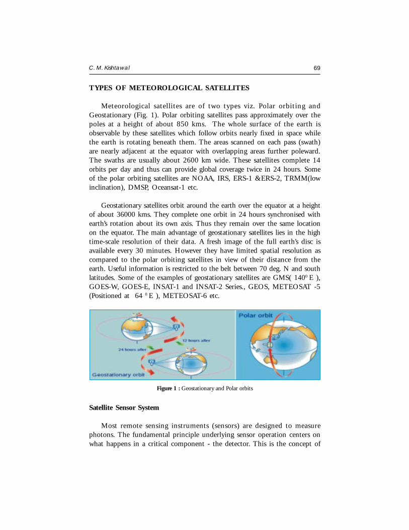
C. M. Kishtawal 69
TYPES OF METEOROLOGICAL SATELLITES
Meteorological satellites are of two types viz. Polar orbiting andGeostationary (Fig. 1). Polar orbiting satellites pass approximately over thepoles at a height of about 850 kms. The whole surface of the earth isobservable by these satellites which follow orbits nearly fixed in space whilethe earth is rotating beneath them. The areas scanned on each pass (swath)are nearly adjacent at the equator with overlapping areas further poleward.The swaths are usually about 2600 km wide. These satellites complete 14orbits per day and thus can provide global coverage twice in 24 hours. Someof the polar orbiting satellites are NOAA, IRS, ERS-1 &ERS-2, TRMM(lowinclination), DMSP, Oceansat-1 etc.
Geostationary satellites orbit around the earth over the equator at a heightof about 36000 kms. They complete one orbit in 24 hours synchronised withearth’s rotation about its own axis. Thus they remain over the same locationon the equator. The main advantage of geostationary satellites lies in the hightime-scale resolution of their data. A fresh image of the full earth’s disc isavailable every 30 minutes. However they have limited spatial resolution ascompared to the polar orbiting satellites in view of their distance from theearth. Useful information is restricted to the belt between 70 deg. N and southlatitudes. Some of the examples of geostationary satellites are GMS( 1400 E ),GOES-W, GOES-E, INSAT-1 and INSAT-2 Series., GEOS, METEOSAT -5(Positioned at 64 0 E ), METEOSAT-6 etc.
Figure 1 : Geostationary and Polar orbits
Satellite Sensor System
Most remote sensing instruments (sensors) are designed to measurephotons. The fundamental principle underlying sensor operation centers onwhat happens in a critical component - the detector. This is the concept of
70 Meteorological satellites
the photoelectric effect (for which Albert Einstein, who first explained it in detail,won his Nobel Prize). This, simply stated, says that there will be an emissionof negative particles (electrons) when a negatively charged plate of someappropriate light-sensitive material is subjected to a beam of photons. Theelectrons can then be made to flow from the plate, collected, and counted asa signal. A key point: The magnitude of the electric current produced (numberof photoelectrons per unit time) is directly proportional to the light intensity.Thus, changes in the electric current can be used to measure changes in thephotons (numbers; intensity) that strike the plate (detector) during a giventime interval. The kinetic energy of the released photoelectrons varies withfrequency (or wavelength) of the impinging radiation. But, different materialsundergo photoelectric effect release of electrons over different wavelengthintervals; each has a threshold wavelength at which the phenomenon beginsand a longer wavelength at which it ceases. Meteorological satellite sensorscan be broadly classified as two types : passive and active (Fig. 2). Passive sensorsdo not use their own source of electromagnetic illumination, and depend uponthe radiation emitted or reflected from the object of interest. On the otherhand, active instruments use their own source of electromagnetic radiationwhich they use to illuminate the target, and in most cases use the propertiesof reflected radiation ( e.g. intensity, polarization, and time delay etc.) todeduce the information about the target. These sensors can be further sub-divided into the following categories and subcategories :
Equally important is the functional classification of these sensors.Meteorological satellite sensors may be deployed to obtain one and/or moreof the following characteristics of different objects of the land-ocean-atmosphere system :
(a) Spatial Information : The examples are the extent and temperature of seasurface, clouds, vegetation, soil moisture, etc. The main objective here isto obtain the required information over a 2-dimensional plane. The bestsuited sensors for this class are imaging radiometers operating in visible,infrared or microwave frequencies. Active sensors like Synthetic ApertureRadar (SAR) are also put to effective use for the imaging applications.
(b) Spectral Information : For certain applications, the spectral details of anelectromagnetic signal are of crucial importance. A particular object ofinterest, for example an atmospheric layer, or, the ocean surface, interactsdifferently with different wavelengths of electromagnetic(EM) spectra. Inmost cases, this may be due to the chemical composition of the object.
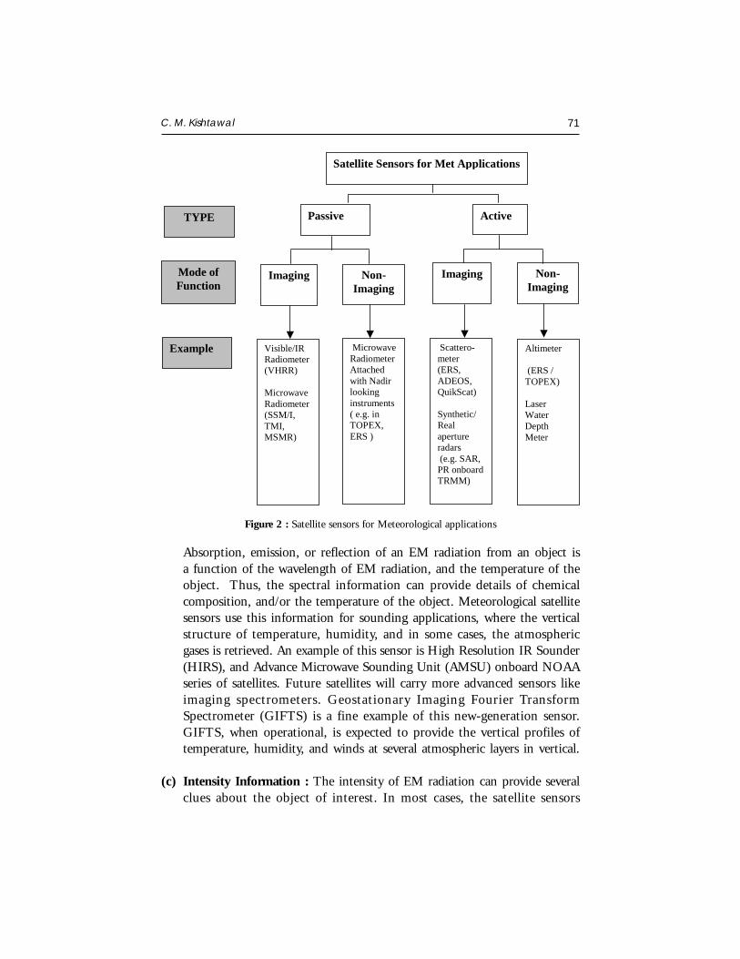
C. M. Kishtawal 71
Absorption, emission, or reflection of an EM radiation from an object isa function of the wavelength of EM radiation, and the temperature of theobject. Thus, the spectral information can provide details of chemicalcomposition, and/or the temperature of the object. Meteorological satellitesensors use this information for sounding applications, where the verticalstructure of temperature, humidity, and in some cases, the atmosphericgases is retrieved. An example of this sensor is High Resolution IR Sounder(HIRS), and Advance Microwave Sounding Unit (AMSU) onboard NOAAseries of satellites. Future satellites will carry more advanced sensors likeimaging spectrometers. Geostationary Imaging Fourier TransformSpectrometer (GIFTS) is a fine example of this new-generation sensor.GIFTS, when operational, is expected to provide the vertical profiles oftemperature, humidity, and winds at several atmospheric layers in vertical.
(c) Intensity Information : The intensity of EM radiation can provide severalclues about the object of interest. In most cases, the satellite sensors
Satellite Sensors for Met Applications
Active Passive TYPE
Mode of Function
Imaging Non-Imaging
Imaging Non-Imaging
Example Visible/IR Radiometer (VHRR) Microwave Radiometer (SSM/I, TMI, MSMR)
Microwave Radiometer Attached with Nadir looking instruments ( e.g. in TOPEX, ERS )
Scattero-meter (ERS, ADEOS, QuikScat) Synthetic/ Real aperture radars (e.g. SAR, PR onboard TRMM)
Altimeter (ERS / TOPEX) Laser Water Depth Meter
Figure 2 : Satellite sensors for Meteorological applications
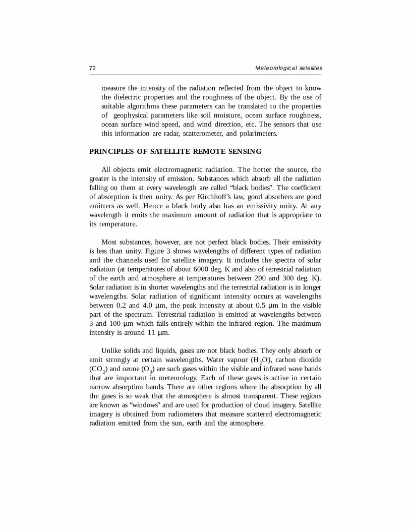
72 Meteorological satellites
measure the intensity of the radiation reflected from the object to knowthe dielectric properties and the roughness of the object. By the use ofsuitable algorithms these parameters can be translated to the propertiesof geophysical parameters like soil moisture, ocean surface roughness,ocean surface wind speed, and wind direction, etc. The sensors that usethis information are radar, scatterometer, and polarimeters.
PRINCIPLES OF SATELLITE REMOTE SENSING
All objects emit electromagnetic radiation. The hotter the source, thegreater is the intensity of emission. Substances which absorb all the radiationfalling on them at every wavelength are called “black bodies”. The coefficientof absorption is then unity. As per Kirchhoff ’s law, good absorbers are goodemitters as well. Hence a black body also has an emissivity unity. At anywavelength it emits the maximum amount of radiation that is appropriate toits temperature.
Most substances, however, are not perfect black bodies. Their emissivityis less than unity. Figure 3 shows wavelengths of different types of radiationand the channels used for satellite imagery. It includes the spectra of solarradiation (at temperatures of about 6000 deg. K and also of terrestrial radiationof the earth and atmosphere at temperatures between 200 and 300 deg. K).Solar radiation is in shorter wavelengths and the terrestrial radiation is in longerwavelengths. Solar radiation of significant intensity occurs at wavelengthsbetween 0.2 and 4.0 µm, the peak intensity at about 0.5 µm in the visiblepart of the spectrum. Terrestrial radiation is emitted at wavelengths between3 and 100 µm which falls entirely within the infrared region. The maximumintensity is around 11 µm.
Unlike solids and liquids, gases are not black bodies. They only absorb oremit strongly at certain wavelengths. Water vapour (H2O), carbon dioxide(CO2) and ozone (O3) are such gases within the visible and infrared wave bandsthat are important in meteorology. Each of these gases is active in certainnarrow absorption bands. There are other regions where the absorption by allthe gases is so weak that the atmosphere is almost transparent. These regionsare known as “windows” and are used for production of cloud imagery. Satelliteimagery is obtained from radiometers that measure scattered electromagneticradiation emitted from the sun, earth and the atmosphere.
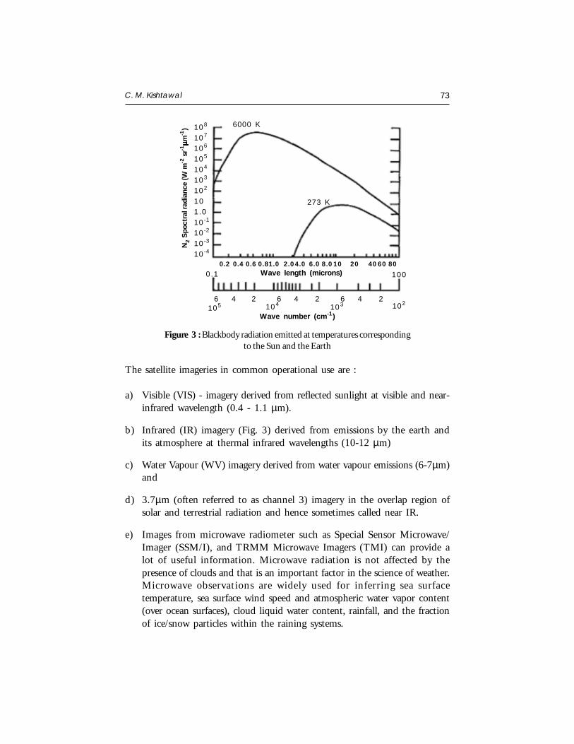
C. M. Kishtawal 73
The satellite imageries in common operational use are :
a) Visible (VIS) - imagery derived from reflected sunlight at visible and near-infrared wavelength (0.4 - 1.1 µm).
b) Infrared (IR) imagery (Fig. 3) derived from emissions by the earth andits atmosphere at thermal infrared wavelengths (10-12 µm)
c) Water Vapour (WV) imagery derived from water vapour emissions (6-7µm)and
d) 3.7µm (often referred to as channel 3) imagery in the overlap region ofsolar and terrestrial radiation and hence sometimes called near IR.
e) Images from microwave radiometer such as Special Sensor Microwave/Imager (SSM/I), and TRMM Microwave Imagers (TMI) can provide alot of useful information. Microwave radiation is not affected by thepresence of clouds and that is an important factor in the science of weather.Microwave observations are widely used for inferring sea surfacetemperature, sea surface wind speed and atmospheric water vapor content(over ocean surfaces), cloud liquid water content, rainfall, and the fractionof ice/snow particles within the raining systems.
Figure 3 : Blackbody radiation emitted at temperatures correspondingto the Sun and the Earth
108
107
106
105
104
103
102
101.010-1
10-2
10-3
10-4
N2 S
poct
ral r
adia
nce
(W m
-2 s
r-1µµµµ µm
-1) 6000 K
273 K
6 4 2 6 4 2 6 4 2105 104 103 102
Wave number (cm-1)
Wave length (microns)0.2 0.4 0.6 0.81.0 2.04.0 6.0 8.010 20 4060 80
0.1 100
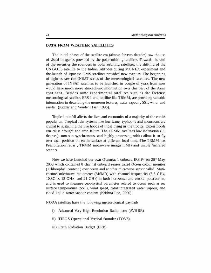
74 Meteorological satellites
DATA FROM WEATHER SATELLITES
The initial phases of the satellite era (almost for two decades) saw the useof visual imageries provided by the polar orbiting satellites. Towards the endof the seventies the sounders in polar orbiting satellites, the shifting of theUS GOES satellite to the Indian latitudes during MONEX experiment andthe launch of Japanese GMS satellites provided new avenues. The beginningof eighties saw the INSAT series of the meteorological satellites. The newgeneration of INSAT satellites to be launched in couple of years from nowwould have much more atmospheric information over this part of the Asiancontinent. Besides some experimental satellites such as the Defensemeteorological satellite, ERS-1 and satellite like TRMM, are providing valuableinformation in describing the monsoon features, water vapour , SST, wind andrainfall (Kidder and Vonder Haar, 1995).
Tropical rainfall affects the lives and economies of a majority of the earth’spopulation. Tropical rain systems like hurricane, typhoons and monsoons arecrucial to sustaining the live hoods of those living in the tropics. Excess floodscan cause drought and crop failure. The TRMM satellite’s low inclination (35degrees), non-sun synchronous, and highly processing orbits allow it to flyover each position on earths surface at different local time. The TRMM hasPrecipitation radar , TRMM microwave imager(TMI) and visible /infraredscanner.
Now we have launched our own Oceansat-1 onboard IRS-P4 on 26th May,2003 which contained 8 channel onboard sensor called Ocean colour monitor( Chlorophyll content ) over ocean and another microwave sensor called Muti-channel microwave radiometer (MSMR) with channel frequencies (6.6 GHz,10.8Ghz, 18 GHz and 21 GHz) in both horizontal and vertical polarization,and is used to measure geophysical parameter related to ocean such as seasurface temperature (SST), wind speed, total integrated water vapour, andcloud liquid water vapour content (Krishna Rao, 2000).
NOAA satellites have the following meteorological payloads
i) Advanced Very High Resolution Radiometer (AVHRR)
ii) TIROS Operational Vertical Sounder (TOVS)
iii) Earth Radiation Budget (ERB)
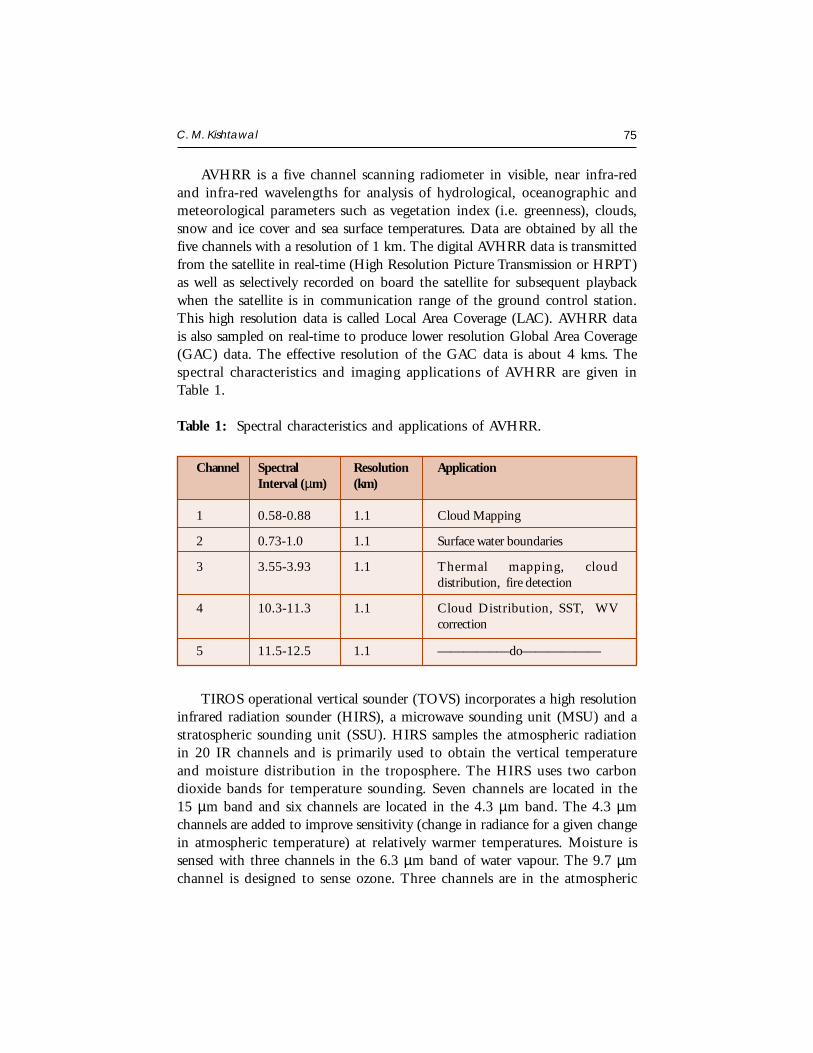
C. M. Kishtawal 75
AVHRR is a five channel scanning radiometer in visible, near infra-redand infra-red wavelengths for analysis of hydrological, oceanographic andmeteorological parameters such as vegetation index (i.e. greenness), clouds,snow and ice cover and sea surface temperatures. Data are obtained by all thefive channels with a resolution of 1 km. The digital AVHRR data is transmittedfrom the satellite in real-time (High Resolution Picture Transmission or HRPT)as well as selectively recorded on board the satellite for subsequent playbackwhen the satellite is in communication range of the ground control station.This high resolution data is called Local Area Coverage (LAC). AVHRR datais also sampled on real-time to produce lower resolution Global Area Coverage(GAC) data. The effective resolution of the GAC data is about 4 kms. Thespectral characteristics and imaging applications of AVHRR are given inTable 1.
Table 1: Spectral characteristics and applications of AVHRR.
Channel Spectral Resolution ApplicationInterval (µm) (km)
1 0.58-0.88 1.1 Cloud Mapping
2 0.73-1.0 1.1 Surface water boundaries
3 3.55-3.93 1.1 Thermal mapping, clouddistribution, fire detection
4 10.3-11.3 1.1 Cloud Distribution, SST, WVcorrection
5 11.5-12.5 1.1 ————–—do——————
TIROS operational vertical sounder (TOVS) incorporates a high resolutioninfrared radiation sounder (HIRS), a microwave sounding unit (MSU) and astratospheric sounding unit (SSU). HIRS samples the atmospheric radiationin 20 IR channels and is primarily used to obtain the vertical temperatureand moisture distribution in the troposphere. The HIRS uses two carbondioxide bands for temperature sounding. Seven channels are located in the15 µm band and six channels are located in the 4.3 µm band. The 4.3 µmchannels are added to improve sensitivity (change in radiance for a given changein atmospheric temperature) at relatively warmer temperatures. Moisture issensed with three channels in the 6.3 µm band of water vapour. The 9.7 µmchannel is designed to sense ozone. Three channels are in the atmospheric
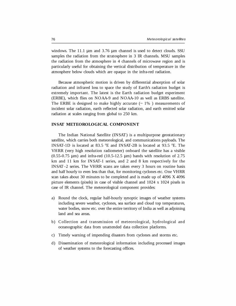
76 Meteorological satellites
windows. The 11.1 µm and 3.76 µm channel is used to detect clouds. SSUsamples the radiation from the stratosphere in 3 IR channels. MSU samplesthe radiation from the atmosphere in 4 channels of microwave region and isparticularly useful for obtaining the vertical distribution of temperature in theatmosphere below clouds which are opaque in the infra-red radiation.
Because atmospheric motion is driven by differential absorption of solarradiation and infrared loss to space the study of Earth’s radiation budget isextremely important. The latest is the Earth radiation budget experiment(ERBE), which flies on NOAA-9 and NOAA-10 as well as ERBS satellite.The ERBE is designed to make highly accurate (~ 1% ) measurements ofincident solar radiation, earth reflected solar radiation, and earth emitted solarradiation at scales ranging from global to 250 km.
INSAT METEOROLOGICAL COMPONENT
The Indian National Satellite (INSAT) is a multipurpose geostationarysatellite, which carries both meteorological, and communications payloads. TheINSAT-1D is located at 83.5 0E and INSAT-2B is located at 93.5 0E. TheVHRR (very high resolution radiometer) onboard the satellite has a visible(0.55-0.75 µm) and infra-red (10.5-12.5 µm) bands with resolution of 2.75km and 11 km for INSAT-1 series, and 2 and 8 km respectively for theINSAT–2 series. The VHRR scans are taken every 3 hours on routine basisand half hourly to even less than that, for monitoring cyclones etc. One VHRRscan takes about 30 minutes to be completed and is made up of 4096 X 4096picture elements (pixels) in case of visible channel and 1024 x 1024 pixels incase of IR channel. The meteorological component provides:
a) Round the clock, regular half-hourly synoptic images of weather systemsincluding severe weather, cyclones, sea surface and cloud top temperatures,water bodies, snow etc. over the entire territory of India as well as adjoiningland and sea areas.
b) Collection and transmission of meteorological, hydrological andoceanographic data from unattended data collection platforms.
c) Timely warning of impending disasters from cyclones and storms etc.
d) Dissemination of meteorological information including processed imagesof weather systems to the forecasting offices.
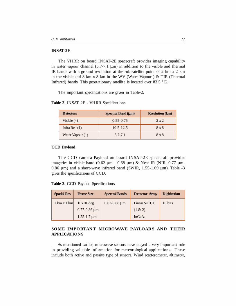
C. M. Kishtawal 77
INSAT-2E
The VHRR on board INSAT-2E spacecraft provides imaging capabilityin water vapour channel (5.7-7.1 µm) in addition to the visible and thermalIR bands with a ground resolution at the sub-satellite point of 2 km x 2 kmin the visible and 8 km x 8 km in the WV (Water Vapour ) & TIR (ThermalInfrared) bands. This geostationary satellite is located over 83.5 0 E.
The important specifications are given in Table-2.
Table 2. INSAT 2E - VHRR Specifications
Detectors Spectral Band (µµµµµm) Resolution (km)
Visible (4) 0.55-0.75 2 x 2
Infra Red (1) 10.5-12.5 8 x 8
Water Vapour (1) 5.7-7.1 8 x 8
CCD Payload
The CCD camera Payload on board INSAT-2E spacecraft providesimageries in visible band (0.62 µm - 0.68 µm) & Near IR (NIR, 0.77 µm-0.86 µm) and a short-wave infrared band (SWIR, 1.55-1.69 µm). Table -3gives the specifications of CCD.
Table 3. CCD Payload Specifications
Spatial Res. Frame Size Spectral Bands Detector Array Digitization
1 km x 1 km 10x10 deg 0.63-0.68 µm Linear Si CCD 10 bits
0.77-0.86 µm (1 & 2)
1.55-1.7 µm InGaAs
SOME IMPORTANT MICROWAVE PAYLOADS AND THEIRAPPLICATIONS
As mentioned earlier, microwave sensors have played a very important rolein providing valuable information for meteorological applications. Theseinclude both active and passive type of sensors. Wind scatterometer, altimeter,
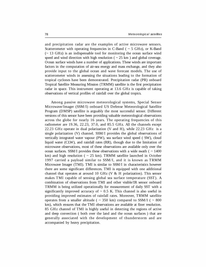
78 Meteorological satellites
and precipitation radar are the examples of active microwave sensors.Scatterometer with operating frequencies in C-Band ( ~ 5 GHz), or K-Band(~ 13 GHz) is an indispensable tool for monitoring the ocean surface windspeed and wind direction with high resolution ( ~ 25 km ) and global coverage.Ocean surface winds have a number of applications. These winds are importantfactors in the computation of air-sea energy and mass exchange, and they alsoprovide input to the global ocean and wave forecast models. The use ofscatterometer winds in assessing the situations leading to the formation oftropical cyclones have been demonstrated. Precipitation radar (PR) onboardTropical Satellite Measuring Mission (TRMM) satellite is the first precipitationradar in space. This instrument operating at 13.6 GHz is capable of takingobservations of vertical profiles of rainfall over the global tropics.
Among passive microwave meteorological systems, Special SensorMicrowave/Imager (SSM/I) onboard US Defense Meteorological SatelliteProgram (DMSP) satellite is arguably the most successful sensor. Differentversions of this sensor have been providing valuable meteorological observationsacross the globe for nearly 16 years. The operating frequencies of thisradiometer are 19.36, 22.23, 37.0, and 85.5 GHz. All the channels except22.23 GHz operate in dual polarization (V and H), while 22.23 GHz is asingle polarization (V) channel. SSM/I provides the global observations ofvertically integrated water vapour (PW), sea surface wind speed ( SW), cloudliquid water (CLW), and rainfall rates (RR), though due to the limitation ofmicrowave observations, most of these observations are available only over theocean surfaces. SSM/I provides these observations with a wide swath ( ~ 1400km) and high resolution ( ~ 25 km). TRMM satellite launched in October1997 carried a payload similar to SSM/I, and it is known as TRMMMicrowave Imager (TMI). TMI is similar to SSM/I in characteristics howeverthere are some significant differences. TMI is equipped with one additionalchannel that operates at around 10 GHz (V & H polarization). This sensormakes TMI capable of sensing global sea surface temperature (SST). Acombination of observations from TMI and other visible/IR sensor onboardTRMM is being utilized operationally for measurement of daily SST with asignificantly improved accuracy of ~ 0.5 K. This channel is also useful inproviding improved estimates of rainfall rates. Moreover, TRMM satelliteoperates from a smaller altitude ( ~ 350 km) compared to SSM/I ( ~ 800km), which ensures that the TMI observations are available at finer resolution.85 GHz channel of TMI is highly useful in detecting the regions of activeand deep convection ( both over the land and the ocean surfaces ) that aregenerally associated with the development of thunderstorm and areaccompanied by heavy precipitation.

C. M. Kishtawal 79
Advance Microwave Sounding Unit ( AMSU) onboard the latest series ofNOAA satellites, is a sounding instrument that provides the temperature andhumidity sounding in presence of clouds, using the absorption bands ofoxygen ( ~ 50 GHz), and water vapour ( ~ 183 GHz) respectively.
CONCLUSIONS
Various kinds of meteorological satellites such as imaging/non-imaging,optical/microwave and passive/active are available for retrieval of meteorologicalparameters, weather forecasting etc. INSAT-VHRR and NOAA-AVHRRsatellites data are very popular in India for studing meteorological conditions.
ACKNOWLEDGEMENTS
I am thankful to my colleague and friend B. Simon who provided a lot ofhelp in the preparation of this lecture. I also acknowledge the valuableinformation I received from the online tutorials by Dr. Nicholas M. Short(email : %[email protected]).
REFERENCES
Kidder, S.Q. and Vonder Haar, T.H. 1995. Satellite Meteorology : An Introduction. AcademicPress.
Krishna Rao, P. 2000. Weather Satellites System Data and Environmental Application.American Meteorological Society, London.
DIGITAL IMAGE PROCESSING
Minakshi KumarPhotogrammetry and Remote Sensing DivisionIndian Institute of Remote Sensing, Dehra Dun
Abstract : This paper describes the basic technological aspects of Digital ImageProcessing with special reference to satellite image processing. Basically, all satelliteimage-processing operations can be grouped into three categories: ImageRectification and Restoration, Enhancement and Information Extraction. The formerdeals with initial processing of raw image data to correct for geometric distortion,to calibrate the data radiometrically and to eliminate noise present in the data.The enhancement procedures are applied to image data in order to effectively displaythe data for subsequent visual interpretation. It involves techniques for increasingthe visual distinction between features in a scene. The objective of the informationextraction operations is to replace visual analysis of the image data with quantitativetechniques for automating the identification of features in a scene. This involvesthe analysis of multispectral image data and the application of statistically baseddecision rules for determining the land cover identity of each pixel in an image.The intent of classification process is to categorize all pixels in a digital image intoone of several land cover classes or themes. This classified data may be used to
produce thematic maps of the land cover present in an image.
INTRODUCTION
Pictures are the most common and convenient means of conveying ortransmitting information. A picture is worth a thousand words. Picturesconcisely convey information about positions, sizes and inter-relationshipsbetween objects. They portray spatial information that we can recognize asobjects. Human beings are good at deriving information from such images,because of our innate visual and mental abilities. About 75% of theinformation received by human is in pictorial form.
In the present context, the analysis of pictures that employ an overheadperspective, including the radiation not visible to human eye are considered.
Satellite Remote Sensing and GIS Applications in Agricultural Meteorologypp. 81-102
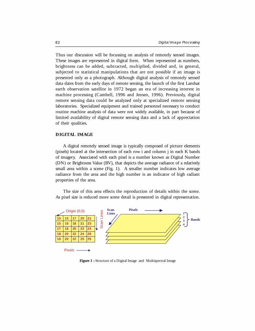
82 Digital Image Processing
Thus our discussion will be focussing on analysis of remotely sensed images.These images are represented in digital form. When represented as numbers,brightness can be added, subtracted, multiplied, divided and, in general,subjected to statistical manipulations that are not possible if an image ispresented only as a photograph. Although digital analysis of remotely senseddata dates from the early days of remote sensing, the launch of the first Landsatearth observation satellite in 1972 began an era of increasing interest inmachine processing (Cambell, 1996 and Jensen, 1996). Previously, digitalremote sensing data could be analyzed only at specialized remote sensinglaboratories. Specialized equipment and trained personnel necessary to conductroutine machine analysis of data were not widely available, in part because oflimited availability of digital remote sensing data and a lack of appreciationof their qualities.
DIGITAL IMAGE
A digital remotely sensed image is typically composed of picture elements(pixels) located at the intersection of each row i and column j in each K bandsof imagery. Associated with each pixel is a number known as Digital Number(DN) or Brightness Value (BV), that depicts the average radiance of a relativelysmall area within a scene (Fig. 1). A smaller number indicates low averageradiance from the area and the high number is an indicator of high radiantproperties of the area.
The size of this area effects the reproduction of details within the scene.As pixel size is reduced more scene detail is presented in digital representation.
Figure 1 : Structure of a Digital Image and Multispectral Image
1 2 3 4
Pixels Scan Lines
Bands
Pixels
Sca
n Li
nes
10 15 17 20 2115 16 18 21 2317 18 20 22 2418 20 22 24 2618 20 22 25 25
Origin (0,0)
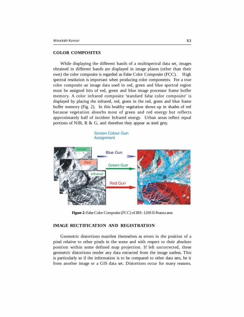
Minakshi Kumar 83
COLOR COMPOSITES
While displaying the different bands of a multispectral data set, imagesobtained in different bands are displayed in image planes (other than theirown) the color composite is regarded as False Color Composite (FCC). Highspectral resolution is important when producing color components. For a truecolor composite an image data used in red, green and blue spectral regionmust be assigned bits of red, green and blue image processor frame buffermemory. A color infrared composite ‘standard false color composite’ isdisplayed by placing the infrared, red, green in the red, green and blue framebuffer memory (Fig. 2). In this healthy vegetation shows up in shades of redbecause vegetation absorbs most of green and red energy but reflectsapproximately half of incident Infrared energy. Urban areas reflect equalportions of NIR, R & G, and therefore they appear as steel grey.
Figure 2: False Color Composite (FCC) of IRS : LISS II Poanta area
IMAGE RECTIFICATION AND REGISTRATION
Geometric distortions manifest themselves as errors in the position of apixel relative to other pixels in the scene and with respect to their absoluteposition within some defined map projection. If left uncorrected, thesegeometric distortions render any data extracted from the image useless. Thisis particularly so if the information is to be compared to other data sets, be itfrom another image or a GIS data set. Distortions occur for many reasons.
Screen Colour GunAssignment
Blue Gun
Green Gun
Red Gun
Green
Infrared
Red
84 Digital Image Processing
For instance distortions occur due to changes in platform attitude (roll, pitchand yaw), altitude, earth rotation, earth curvature, panoramic distortion anddetector delay. Most of these distortions can be modelled mathematically andare removed before you buy an image. Changes in attitude however can bedifficult to account for mathematically and so a procedure called imagerectification is performed. Satellite systems are however geometrically quitestable and geometric rectification is a simple procedure based on a mappingtransformation relating real ground coordinates, say in easting and northing,to image line and pixel coordinates.
Rectification is a process of geometrically correcting an image so that it canbe represented on a planar surface , conform to other images or conform to amap (Fig. 3). That is, it is the process by which geometry of an image is madeplanimetric. It is necessary when accurate area, distance and directionmeasurements are required to be made from the imagery. It is achieved bytransforming the data from one grid system into another grid system using ageometric transformation.
Rectification is not necessary if there is no distortion in the image. Forexample, if an image file is produced by scanning or digitizing a paper mapthat is in the desired projection system, then that image is already planar anddoes not require rectification unless there is some skew or rotation of the image.Scanning and digitizing produce images that are planar, but do not containany map coordinate information. These images need only to be geo-referenced,which is a much simpler process than rectification. In many cases, the imageheader can simply be updated with new map coordinate information. Thisinvolves redefining the map coordinate of the upper left corner of the imageand the cell size (the area represented by each pixel).
Ground Control Points (GCP) are the specific pixels in the input imagefor which the output map coordinates are known. By using more points thannecessary to solve the transformation equations a least squares solution maybe found that minimises the sum of the squares of the errors. Care should beexercised when selecting ground control points as their number, quality anddistribution affect the result of the rectification.
Once the mapping transformation has been determined a procedure calledresampling is employed. Resampling matches the coordinates of image pixelsto their real world coordinates and writes a new image on a pixel by pixelbasis. Since the grid of pixels in the source image rarely matches the grid for
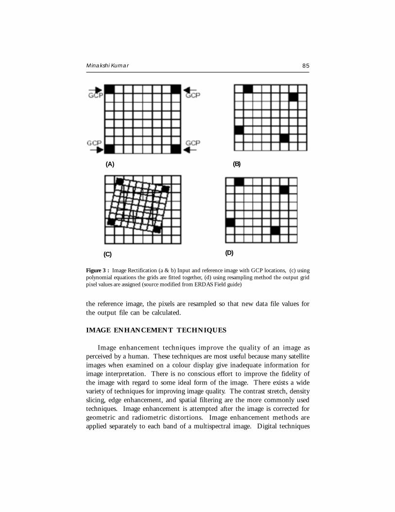
Minakshi Kumar 85
the reference image, the pixels are resampled so that new data file values forthe output file can be calculated.
IMAGE ENHANCEMENT TECHNIQUES
Image enhancement techniques improve the quality of an image asperceived by a human. These techniques are most useful because many satelliteimages when examined on a colour display give inadequate information forimage interpretation. There is no conscious effort to improve the fidelity ofthe image with regard to some ideal form of the image. There exists a widevariety of techniques for improving image quality. The contrast stretch, densityslicing, edge enhancement, and spatial filtering are the more commonly usedtechniques. Image enhancement is attempted after the image is corrected forgeometric and radiometric distortions. Image enhancement methods areapplied separately to each band of a multispectral image. Digital techniques
Figure 3 : Image Rectification (a & b) Input and reference image with GCP locations, (c) usingpolynomial equations the grids are fitted together, (d) using resampling method the output gridpixel values are assigned (source modified from ERDAS Field guide)
(A) (B)
(C) (D)
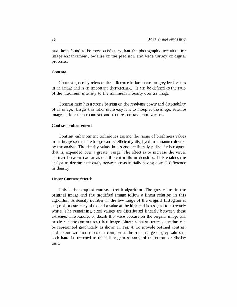
86 Digital Image Processing
have been found to be most satisfactory than the photographic technique forimage enhancement, because of the precision and wide variety of digitalprocesses.
Contrast
Contrast generally refers to the difference in luminance or grey level valuesin an image and is an important characteristic. It can be defined as the ratioof the maximum intensity to the minimum intensity over an image.
Contrast ratio has a strong bearing on the resolving power and detectabilityof an image. Larger this ratio, more easy it is to interpret the image. Satelliteimages lack adequate contrast and require contrast improvement.
Contrast Enhancement
Contrast enhancement techniques expand the range of brightness valuesin an image so that the image can be efficiently displayed in a manner desiredby the analyst. The density values in a scene are literally pulled farther apart,that is, expanded over a greater range. The effect is to increase the visualcontrast between two areas of different uniform densities. This enables theanalyst to discriminate easily between areas initially having a small differencein density.
Linear Contrast Stretch
This is the simplest contrast stretch algorithm. The grey values in theoriginal image and the modified image follow a linear relation in thisalgorithm. A density number in the low range of the original histogram isassigned to extremely black and a value at the high end is assigned to extremelywhite. The remaining pixel values are distributed linearly between theseextremes. The features or details that were obscure on the original image willbe clear in the contrast stretched image. Linear contrast stretch operation canbe represented graphically as shown in Fig. 4. To provide optimal contrastand colour variation in colour composites the small range of grey values ineach band is stretched to the full brightness range of the output or displayunit.
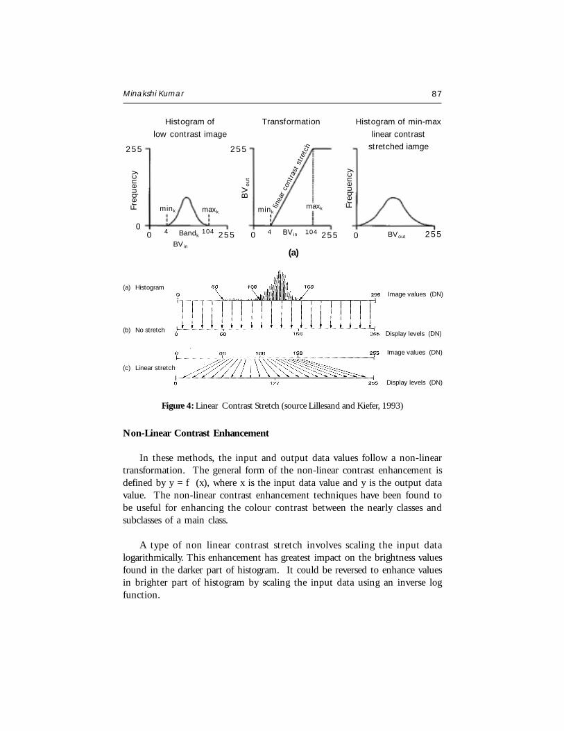
Minakshi Kumar 87
Non-Linear Contrast Enhancement
In these methods, the input and output data values follow a non-lineartransformation. The general form of the non-linear contrast enhancement isdefined by y = f (x), where x is the input data value and y is the output datavalue. The non-linear contrast enhancement techniques have been found tobe useful for enhancing the colour contrast between the nearly classes andsubclasses of a main class.
A type of non linear contrast stretch involves scaling the input datalogarithmically. This enhancement has greatest impact on the brightness valuesfound in the darker part of histogram. It could be reversed to enhance valuesin brighter part of histogram by scaling the input data using an inverse logfunction.
Figure 4: Linear Contrast Stretch (source Lillesand and Kiefer, 1993)
Histogram oflow contrast image
Transformation Histogram of min-maxlinear contrast
stretched iamge
Freq
uenc
y
255
0
mink
linea
r co
ntra
st s
tret
ch
maxkmink maxk
Freq
uenc
y
BV
out
255
00 255 255 25504 104Bandk4 104BVin BVout
BVin
(a)
Image values (DN)
Display levels (DN)
Image values (DN)
Display levels (DN)
(a) Histogram
(b) No stretch
(c) Linear stretch
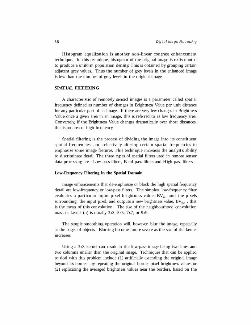
88 Digital Image Processing
Histogram equalization is another non-linear contrast enhancementtechnique. In this technique, histogram of the original image is redistributedto produce a uniform population density. This is obtained by grouping certainadjacent grey values. Thus the number of grey levels in the enhanced imageis less than the number of grey levels in the original image.
SPATIAL FILTERING
A characteristic of remotely sensed images is a parameter called spatialfrequency defined as number of changes in Brightness Value per unit distancefor any particular part of an image. If there are very few changes in BrightnessValue once a given area in an image, this is referred to as low frequency area.Conversely, if the Brightness Value changes dramatically over short distances,this is an area of high frequency.
Spatial filtering is the process of dividing the image into its constituentspatial frequencies, and selectively altering certain spatial frequencies toemphasize some image features. This technique increases the analyst’s abilityto discriminate detail. The three types of spatial filters used in remote sensordata processing are : Low pass filters, Band pass filters and High pass filters.
Low-Frequency Filtering in the Spatial Domain
Image enhancements that de-emphasize or block the high spatial frequencydetail are low-frequency or low-pass filters. The simplest low-frequency filterevaluates a particular input pixel brightness value, BVin, and the pixelssurrounding the input pixel, and outputs a new brightness value, BVout , thatis the mean of this convolution. The size of the neighbourhood convolutionmask or kernel (n) is usually 3x3, 5x5, 7x7, or 9x9.
The simple smoothing operation will, however, blur the image, especiallyat the edges of objects. Blurring becomes more severe as the size of the kernelincreases.
Using a 3x3 kernel can result in the low-pass image being two lines andtwo columns smaller than the original image. Techniques that can be appliedto deal with this problem include (1) artificially extending the original imagebeyond its border by repeating the original border pixel brightness values or(2) replicating the averaged brightness values near the borders, based on the
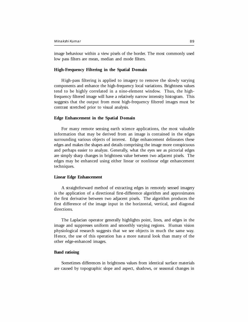
Minakshi Kumar 89
image behaviour within a view pixels of the border. The most commonly usedlow pass filters are mean, median and mode filters.
High-Frequency Filtering in the Spatial Domain
High-pass filtering is applied to imagery to remove the slowly varyingcomponents and enhance the high-frequency local variations. Brightness valuestend to be highly correlated in a nine-element window. Thus, the high-frequency filtered image will have a relatively narrow intensity histogram. Thissuggests that the output from most high-frequency filtered images must becontrast stretched prior to visual analysis.
Edge Enhancement in the Spatial Domain
For many remote sensing earth science applications, the most valuableinformation that may be derived from an image is contained in the edgessurrounding various objects of interest. Edge enhancement delineates theseedges and makes the shapes and details comprising the image more conspicuousand perhaps easier to analyze. Generally, what the eyes see as pictorial edgesare simply sharp changes in brightness value between two adjacent pixels. Theedges may be enhanced using either linear or nonlinear edge enhancementtechniques.
Linear Edge Enhancement
A straightforward method of extracting edges in remotely sensed imageryis the application of a directional first-difference algorithm and approximatesthe first derivative between two adjacent pixels. The algorithm produces thefirst difference of the image input in the horizontal, vertical, and diagonaldirections.
The Laplacian operator generally highlights point, lines, and edges in theimage and suppresses uniform and smoothly varying regions. Human visionphysiological research suggests that we see objects in much the same way.Hence, the use of this operation has a more natural look than many of theother edge-enhanced images.
Band ratioing
Sometimes differences in brightness values from identical surface materialsare caused by topographic slope and aspect, shadows, or seasonal changes in
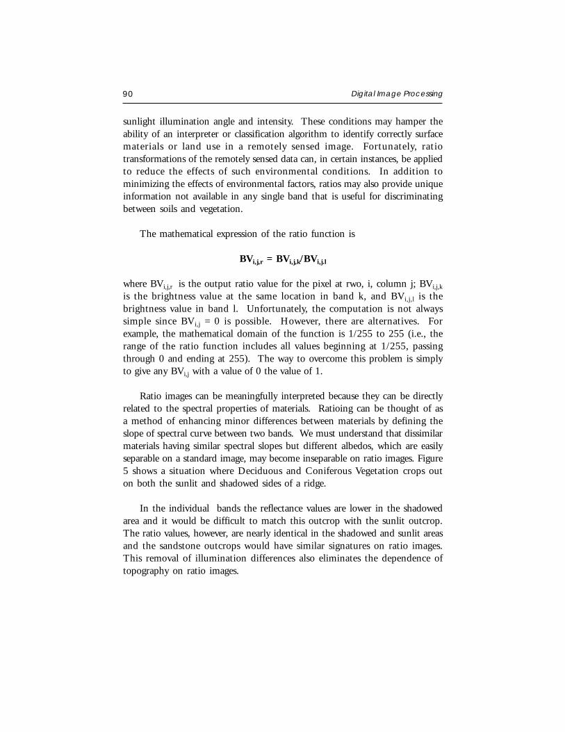
90 Digital Image Processing
sunlight illumination angle and intensity. These conditions may hamper theability of an interpreter or classification algorithm to identify correctly surfacematerials or land use in a remotely sensed image. Fortunately, ratiotransformations of the remotely sensed data can, in certain instances, be appliedto reduce the effects of such environmental conditions. In addition tominimizing the effects of environmental factors, ratios may also provide uniqueinformation not available in any single band that is useful for discriminatingbetween soils and vegetation.
The mathematical expression of the ratio function is
BVi,j,r = BVi,j,k/BVi,j.l
where BVi,j,r is the output ratio value for the pixel at rwo, i, column j; BVi,j,k
is the brightness value at the same location in band k, and BVi,j,l is thebrightness value in band l. Unfortunately, the computation is not alwayssimple since BVi,j = 0 is possible. However, there are alternatives. Forexample, the mathematical domain of the function is 1/255 to 255 (i.e., therange of the ratio function includes all values beginning at 1/255, passingthrough 0 and ending at 255). The way to overcome this problem is simplyto give any BVi,j with a value of 0 the value of 1.
Ratio images can be meaningfully interpreted because they can be directlyrelated to the spectral properties of materials. Ratioing can be thought of asa method of enhancing minor differences between materials by defining theslope of spectral curve between two bands. We must understand that dissimilarmaterials having similar spectral slopes but different albedos, which are easilyseparable on a standard image, may become inseparable on ratio images. Figure5 shows a situation where Deciduous and Coniferous Vegetation crops outon both the sunlit and shadowed sides of a ridge.
In the individual bands the reflectance values are lower in the shadowedarea and it would be difficult to match this outcrop with the sunlit outcrop.The ratio values, however, are nearly identical in the shadowed and sunlit areasand the sandstone outcrops would have similar signatures on ratio images.This removal of illumination differences also eliminates the dependence oftopography on ratio images.
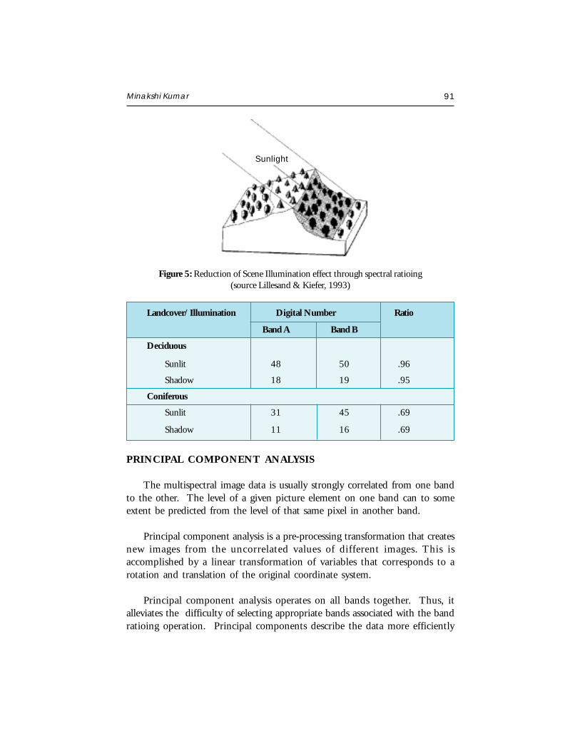
Minakshi Kumar 91
Landcover/ Illumination Digital Number Ratio
Band A Band B
Deciduous
Sunlit 48 50 .96
Shadow 18 19 .95
Coniferous
Sunlit 31 45 .69
Shadow 11 16 .69
PRINCIPAL COMPONENT ANALYSIS
The multispectral image data is usually strongly correlated from one bandto the other. The level of a given picture element on one band can to someextent be predicted from the level of that same pixel in another band.
Principal component analysis is a pre-processing transformation that createsnew images from the uncorrelated values of different images. This isaccomplished by a linear transformation of variables that corresponds to arotation and translation of the original coordinate system.
Principal component analysis operates on all bands together. Thus, italleviates the difficulty of selecting appropriate bands associated with the bandratioing operation. Principal components describe the data more efficiently
Figure 5: Reduction of Scene Illumination effect through spectral ratioing(source Lillesand & Kiefer, 1993)
Sunlight
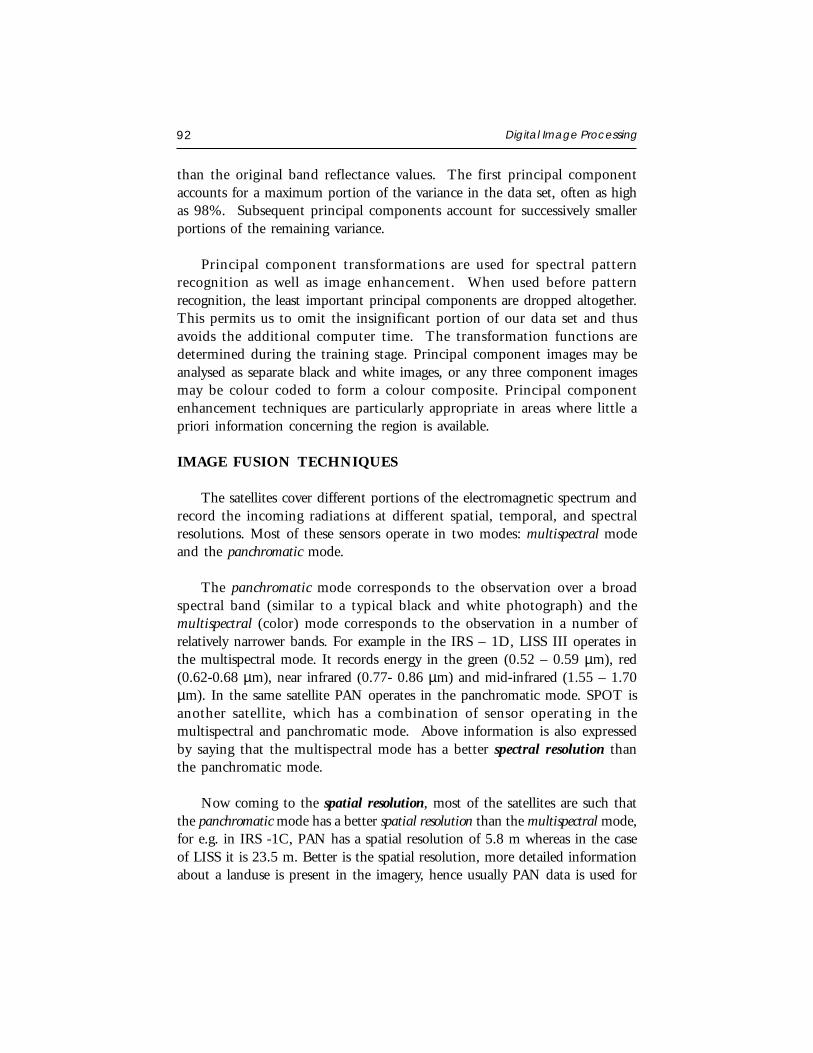
92 Digital Image Processing
than the original band reflectance values. The first principal componentaccounts for a maximum portion of the variance in the data set, often as highas 98%. Subsequent principal components account for successively smallerportions of the remaining variance.
Principal component transformations are used for spectral patternrecognition as well as image enhancement. When used before patternrecognition, the least important principal components are dropped altogether.This permits us to omit the insignificant portion of our data set and thusavoids the additional computer time. The transformation functions aredetermined during the training stage. Principal component images may beanalysed as separate black and white images, or any three component imagesmay be colour coded to form a colour composite. Principal componentenhancement techniques are particularly appropriate in areas where little apriori information concerning the region is available.
IMAGE FUSION TECHNIQUES
The satellites cover different portions of the electromagnetic spectrum andrecord the incoming radiations at different spatial, temporal, and spectralresolutions. Most of these sensors operate in two modes: multispectral modeand the panchromatic mode.
The panchromatic mode corresponds to the observation over a broadspectral band (similar to a typical black and white photograph) and themultispectral (color) mode corresponds to the observation in a number ofrelatively narrower bands. For example in the IRS – 1D, LISS III operates inthe multispectral mode. It records energy in the green (0.52 – 0.59 µm), red(0.62-0.68 µm), near infrared (0.77- 0.86 µm) and mid-infrared (1.55 – 1.70µm). In the same satellite PAN operates in the panchromatic mode. SPOT isanother satellite, which has a combination of sensor operating in themultispectral and panchromatic mode. Above information is also expressedby saying that the multispectral mode has a better spectral resolution thanthe panchromatic mode.
Now coming to the spatial resolution, most of the satellites are such thatthe panchromatic mode has a better spatial resolution than the multispectral mode,for e.g. in IRS -1C, PAN has a spatial resolution of 5.8 m whereas in the caseof LISS it is 23.5 m. Better is the spatial resolution, more detailed informationabout a landuse is present in the imagery, hence usually PAN data is used for
Minakshi Kumar 93
observing and separating various feature. Both theses type of sensors have theirparticular utility as per the need of user. If the need of the user is to separatetwo different kind of landuses, LISS III is used, whereas for a detailed mappreparation of any area, PAN imagery is extremely useful.
Image Fusion is the combination of two or more different images to forma new image (by using a certain algorithm).
The commonly applied Image Fusion Techniques are
1. IHS Transformation
2. PCA
3. Brovey Transform
4. Band Substitution
IMAGE CLASSIFICATION
The overall objective of image classification is to automatically categorizeall pixels in an image into land cover classes or themes. Normally, multispectraldata are used to perform the classification, and the spectral pattern presentwithin the data for each pixel is used as numerical basis for categorization.That is, different feature types manifest different combination of DNs basedon their inherent spectral reflectance and emittance properties.
The term classifier refers loosely to a computer program that implementsa specific procedure for image classification. Over the years scientists havedevised many classification strategies. From these alternatives the analyst mustselect the classifier that will best accomplish a specific task. At present it isnot possible to state that a given classifier is “best” for all situations becausecharacteristics of each image and the circumstances for each study vary sogreatly. Therefore, it is essential that the analyst understands the alternativestrategies for image classification.
The traditional methods of classification mainly follow two approaches:unsupervised and supervised. The unsupervised approach attempts spectralgrouping that may have an unclear meaning from the user’s point of view.Having established these, the analyst then tries to associate an informationclass with each group. The unsupervised approach is often referred to as
94 Digital Image Processing
clustering and results in statistics that are for spectral, statistical clusters. Inthe supervised approach to classification, the image analyst supervises the pixelcategorization process by specifying to the computer algorithm; numericaldescriptors of the various land cover types present in the scene. To do this,representative sample sites of known cover types, called training areas ortraining sites, are used to compile a numerical interpretation key that describesthe spectral attributes for each feature type of interest. Each pixel in the dataset is then compared numerically to each category in the interpretation keyand labeled with the name of the category it looks most like. In the supervisedapproach the user defines useful information categories and then examines theirspectral separability whereas in the unsupervised approach he first determinesspectrally separable classes and then defines their informational utility.
It has been found that in areas of complex terrain, the unsupervisedapproach is preferable to the supervised one. In such conditions if thesupervised approach is used, the user will have difficulty in selecting trainingsites because of the variability of spectral response within each class.Consequently, a prior ground data collection can be very time consuming.Also, the supervised approach is subjective in the sense that the analyst triesto classify information categories, which are often composed of several spectralclasses whereas spectrally distinguishable classes will be revealed by theunsupervised approach, and hence ground data collection requirements maybe reduced. Additionally, the unsupervised approach has the potentialadvantage of revealing discriminable classes unknown from previous work.However, when definition of representative training areas is possible andstatistical information classes show a close correspondence, the results ofsupervised classification will be superior to unsupervised classification.
Unsupervised classification
Unsupervised classifiers do not utilize training data as the basis forclassification. Rather, this family of classifiers involves algorithms that examinethe unknown pixels in an image and aggregate them into a number of classesbased on the natural groupings or clusters present in the image values. Itperforms very well in cases where the values within a given cover type are closetogether in the measurement space, data in different classes are comparativelywell separated.
The classes that result from unsupervised classification are spectral classesbecause they are based solely on the natural groupings in the image values,
Minakshi Kumar 95
the identity of the spectral classes will not be initially known. The analystmust compare the classified data with some form of reference data (such aslarger scale imagery or maps) to determine the identity and informational valueof the spectral classes. In the supervised approach we define useful informationcategories and then examine their spectral separability; in the unsupervisedapproach we determine spectrally separable classes and then define theirinformational utility.
There are numerous clustering algorithms that can be used to determinethe natural spectral groupings present in data set. One common form ofclustering, called the “K-means” approach also called as ISODATA (InteractionSelf-Organizing Data Analysis Technique) accepts from the analyst the numberof clusters to be located in the data. The algorithm then arbitrarily “seeds”,or locates, that number of cluster centers in the multidimensional measurementspace. Each pixel in the image is then assigned to the cluster whose arbitrarymean vector is closest. After all pixels have been classified in this manner,revised mean vectors for each of the clusters are computed. The revised meansare then used as the basis of reclassification of the image data. The procedurecontinues until there is no significant change in the location of class meanvectors between successive iterations of the algorithm. Once this point isreached, the analyst determines the land cover identity of each spectral class.Because the K-means approach is iterative, it is computationally intensive.Therefore, it is often applied only to image sub-areas rather than to full scenes.
Supervised classification
Supervised classification can be defined normally as the process of samplesof known identity to classify pixels of unknown identity. Samples of knownidentity are those pixels located within training areas. Pixels located withinthese areas term the training samples used to guide the classification algorithmto assigning specific spectral values to appropriate informational class.
The basic steps involved in a typical supervised classification procedureare illustrated on Fig. 6.
The training stageFeature selectionSelection of appropriate classification algorithmPost classification smootheningAccuracy assessment
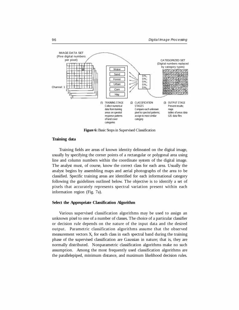
96 Digital Image Processing
Training data
Training fields are areas of known identity delineated on the digital image,usually by specifying the corner points of a rectangular or polygonal area usingline and column numbers within the coordinate system of the digital image.The analyst must, of course, know the correct class for each area. Usually theanalyst begins by assembling maps and aerial photographs of the area to beclassified. Specific training areas are identified for each informational categoryfollowing the guidelines outlined below. The objective is to identify a set ofpixels that accurately represents spectral variation present within eachinformation region (Fig. 7a).
Select the Appropriate Classification Algorithm
Various supervised classification algorithms may be used to assign anunknown pixel to one of a number of classes. The choice of a particular classifieror decision rule depends on the nature of the input data and the desiredoutput. Parametric classification algorithms assume that the observedmeasurement vectors Xc for each class in each spectral band during the trainingphase of the supervised classification are Gaussian in nature; that is, they arenormally distributed. Nonparametric classification algorithms make no suchassumption. Among the most frequently used classification algorithms arethe parallelepiped, minimum distance, and maximum likelihood decision rules.
Figure 6: Basic Steps in Supervised Classification
IMAGE DATA SET(Five digital numbers
per pixel) CATEGORIZED SET(Digital numbers replaced
by category types)
Channel: 12345
(1) TRAINING STAGECollect numericaldata from trainingareas on speotralresponse patternsof land covercategories
(2) CLASSIFICATIONSTAGESCompare each unknownpixel to spectral patterns;assign to most similarcategory
(3) OUTPUT STAGEPresent results;mapstables of areas dataGIS data files
Water
Sand
Forest
Urban
Corn
Hay
DN1DN2DN3DN4DN5
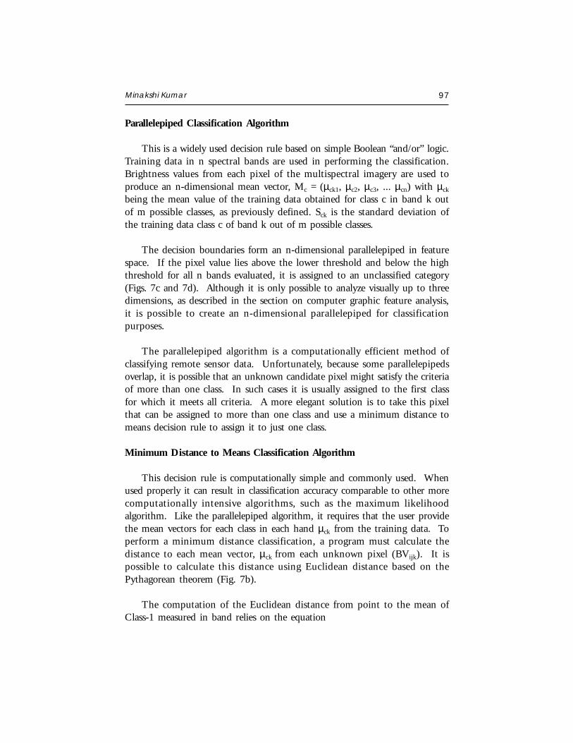
Minakshi Kumar 97
Parallelepiped Classification Algorithm
This is a widely used decision rule based on simple Boolean “and/or” logic.Training data in n spectral bands are used in performing the classification.Brightness values from each pixel of the multispectral imagery are used toproduce an n-dimensional mean vector, Mc = (µck1, µc2, µc3, ... µcn) with µck
being the mean value of the training data obtained for class c in band k outof m possible classes, as previously defined. Sck is the standard deviation ofthe training data class c of band k out of m possible classes.
The decision boundaries form an n-dimensional parallelepiped in featurespace. If the pixel value lies above the lower threshold and below the highthreshold for all n bands evaluated, it is assigned to an unclassified category(Figs. 7c and 7d). Although it is only possible to analyze visually up to threedimensions, as described in the section on computer graphic feature analysis,it is possible to create an n-dimensional parallelepiped for classificationpurposes.
The parallelepiped algorithm is a computationally efficient method ofclassifying remote sensor data. Unfortunately, because some parallelepipedsoverlap, it is possible that an unknown candidate pixel might satisfy the criteriaof more than one class. In such cases it is usually assigned to the first classfor which it meets all criteria. A more elegant solution is to take this pixelthat can be assigned to more than one class and use a minimum distance tomeans decision rule to assign it to just one class.
Minimum Distance to Means Classification Algorithm
This decision rule is computationally simple and commonly used. Whenused properly it can result in classification accuracy comparable to other morecomputationally intensive algorithms, such as the maximum likelihoodalgorithm. Like the parallelepiped algorithm, it requires that the user providethe mean vectors for each class in each hand µck from the training data. Toperform a minimum distance classification, a program must calculate thedistance to each mean vector, µck from each unknown pixel (BVijk). It ispossible to calculate this distance using Euclidean distance based on thePythagorean theorem (Fig. 7b).
The computation of the Euclidean distance from point to the mean ofClass-1 measured in band relies on the equation
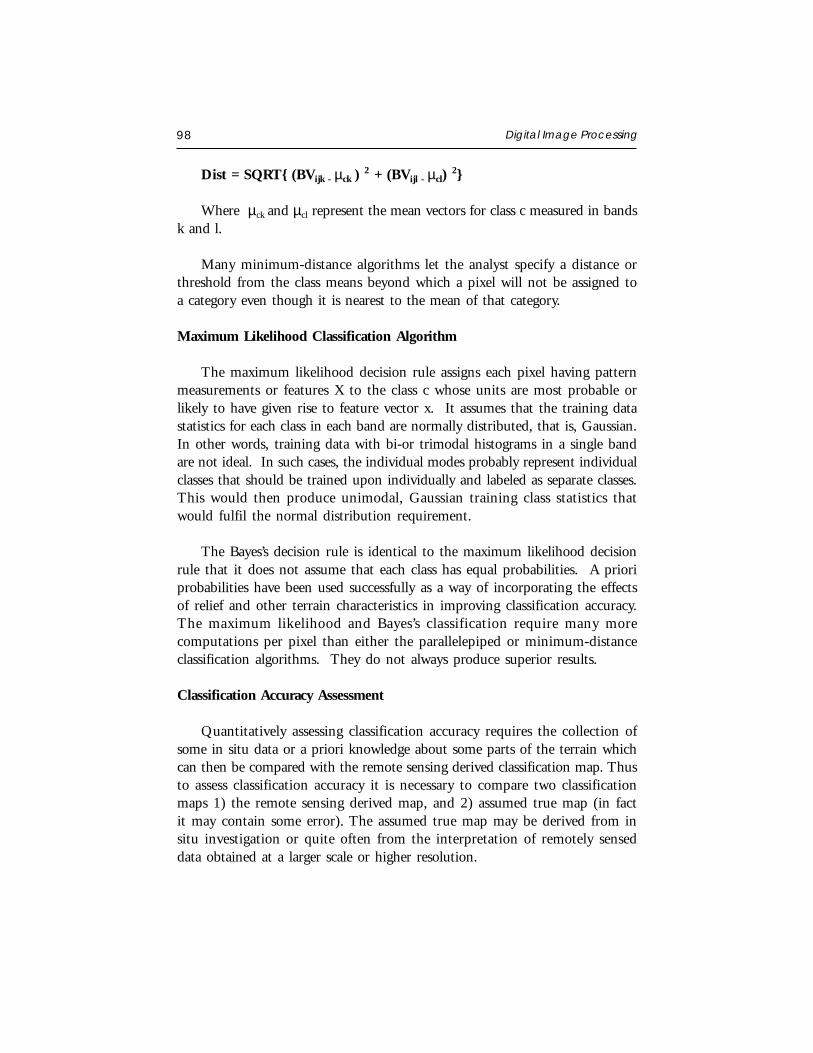
98 Digital Image Processing
Dist = SQRT{ (BVijk - µck ) 2 + (BVijl - µcl)
2}
Where µck and µcl represent the mean vectors for class c measured in bandsk and l.
Many minimum-distance algorithms let the analyst specify a distance orthreshold from the class means beyond which a pixel will not be assigned toa category even though it is nearest to the mean of that category.
Maximum Likelihood Classification Algorithm
The maximum likelihood decision rule assigns each pixel having patternmeasurements or features X to the class c whose units are most probable orlikely to have given rise to feature vector x. It assumes that the training datastatistics for each class in each band are normally distributed, that is, Gaussian.In other words, training data with bi-or trimodal histograms in a single bandare not ideal. In such cases, the individual modes probably represent individualclasses that should be trained upon individually and labeled as separate classes.This would then produce unimodal, Gaussian training class statistics thatwould fulfil the normal distribution requirement.
The Bayes’s decision rule is identical to the maximum likelihood decisionrule that it does not assume that each class has equal probabilities. A prioriprobabilities have been used successfully as a way of incorporating the effectsof relief and other terrain characteristics in improving classification accuracy.The maximum likelihood and Bayes’s classification require many morecomputations per pixel than either the parallelepiped or minimum-distanceclassification algorithms. They do not always produce superior results.
Classification Accuracy Assessment
Quantitatively assessing classification accuracy requires the collection ofsome in situ data or a priori knowledge about some parts of the terrain whichcan then be compared with the remote sensing derived classification map. Thusto assess classification accuracy it is necessary to compare two classificationmaps 1) the remote sensing derived map, and 2) assumed true map (in factit may contain some error). The assumed true map may be derived from insitu investigation or quite often from the interpretation of remotely senseddata obtained at a larger scale or higher resolution.
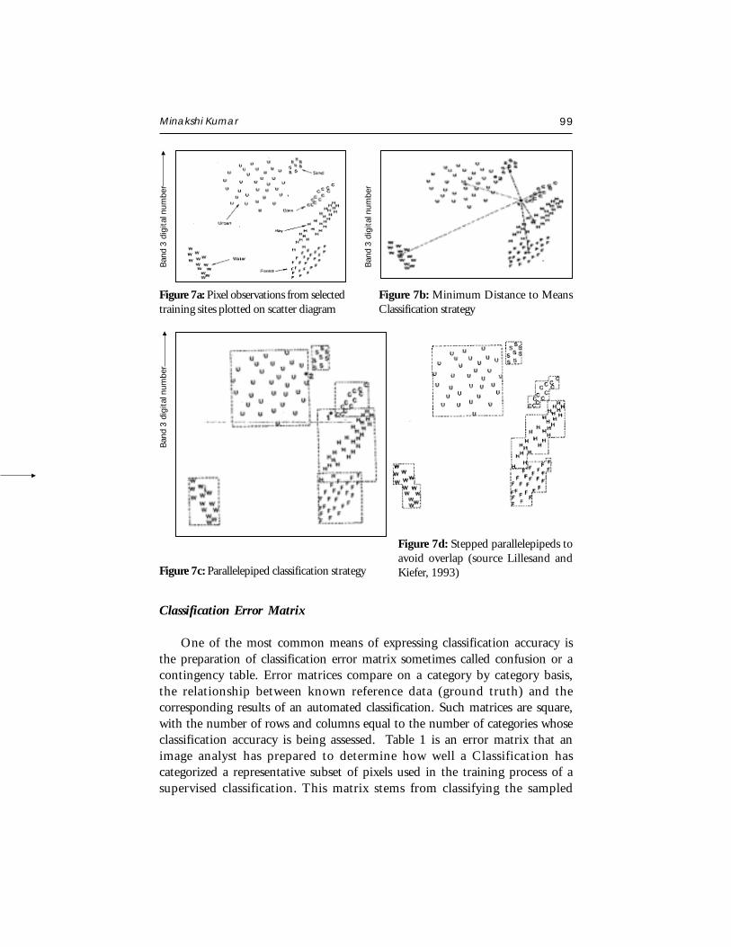
Minakshi Kumar 99
Ban
d 3 d
igita
l num
ber
Ban
d 3 d
igita
l num
ber
Ban
d 3 d
igita
l num
ber
Figure 7a: Pixel observations from selectedtraining sites plotted on scatter diagram
Figure 7b: Minimum Distance to MeansClassification strategy
Figure 7c: Parallelepiped classification strategy
Figure 7d: Stepped parallelepipeds toavoid overlap (source Lillesand andKiefer, 1993)
Classification Error Matrix
One of the most common means of expressing classification accuracy isthe preparation of classification error matrix sometimes called confusion or acontingency table. Error matrices compare on a category by category basis,the relationship between known reference data (ground truth) and thecorresponding results of an automated classification. Such matrices are square,with the number of rows and columns equal to the number of categories whoseclassification accuracy is being assessed. Table 1 is an error matrix that animage analyst has prepared to determine how well a Classification hascategorized a representative subset of pixels used in the training process of asupervised classification. This matrix stems from classifying the sampled
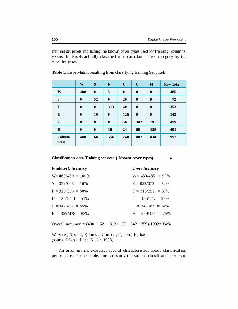
100 Digital Image Processing
training set pixels and listing the known cover types used for training (columns)versus the Pixels actually classified into each land cover category by theclassifier (rows).
Table 1. Error Matrix resulting from classifying training Set pixels
W S F U C H Row Total
W 480 0 5 0 0 0 485
S 0 52 0 20 0 0 72
F 0 0 313 40 0 0 353
U 0 16 0 126 0 0 142
C 0 0 0 38 342 79 459
H 0 0 38 24 60 359 481
Column 480 68 356 248 402 438 1992Total
Classification data Training set data ( Known cover types)
Producer’s Accuracy Users Accuracy
W= 480/480 = 100% W= 480/485 = 99%
S = 052/068 = 16% S = 052/072 = 72%
F = 313/356 = 88% F = 313/352 = 87%
U =126/241l = 51% U = 126/147 = 99%
C = 342/402 = 85% C = 342/459 = 74%
H = 359/438 = 82% H = 359/481 = 75%
Overall accuracy = (480 + 52 + 313+ 126+ 342 +359)/1992= 84%
W, water; S, sand; F, forest; U, urban; C, corn; H, hay(source Lillesand and Kiefer, 1993).
An error matrix expresses several characteristics about classificationperformance. For example, one can study the various classification errors of
Minakshi Kumar 101
omission (exclusion) and commission (inclusion). Note in Table 1 the trainingset pixels that are classified into the proper land cover categories are locatedalong the major diagonal of the error matrix (running from upper left to lowerright). All non-diagonal elements of the matrix represent errors of omissionor commission. Omission errors correspond to non-diagonal column elements(e.g. 16 pixels that should have classified as “sand” were omitted from thatcategory). Commission errors are represented by non-diagonal row elements(e.g. 38 urban pixels plus 79 hay pixels were improperly included in the corncategory).
Several other measures for e.g. the overall accuracy of classification can becomputed from the error matrix. It is determined by dividing the total numbercorrectly classified pixels (sum of elements along the major diagonal) by thetotal number of reference pixels. Likewise, the accuracies of individual categoriescan be calculated by dividing the number of correctly classified pixels in eachcategory by either the total number of pixels in the corresponding rows orcolumn. Producers accuracy which indicates how well the training sets pixelsof a given cover type are classified can be determined by dividing the numberof correctly classified pixels in each category by number of training sets usedfor that category (column total). Users accuracy is computed by dividing thenumber of correctly classified pixels in each category by the total number ofpixels that were classified in that category (row total). This figure is a measureof commission error and indicates the probability that a pixel classified into agiven category actually represents that category on ground.
Note that the error matrix in the table indicates an overall accuracy of84%. However producers accuracy ranges from just 51% (urban) to 100%(water) and users accuracy ranges from 72% (sand) to 99% (water). This errormatrix is based on training data. If the results are good it indicates that thetraining samples are spectrally separable and the classification works well inthe training areas. This aids in the training set refinement process, but indicateslittle about classifier performance else where in the scene.
Kappa coefficient
Kappa analysis is a discrete multivariate technique for accuracy assessment.Kappa analysis yields a Khat statistic that is the measure of agreement ofaccuracy. The Khat statistic is computed as
102 Digital Image Processing
Khat = ∑
∑ ∑
++
+
+−+
rii
r2iiii
r
)*x(xN)*xx(xN
Where r is the number of rows in the matrix xii is the number of observationsin row i and column i, and xi+ and x+i are the marginal totals for the row iand column i respectively and N is the total number of observations.
CONCLUSIONS
Digital image processings of satellite data can be primarily grouped intothree categories : Image Rectification and Restoration, Enhancement andInformation extraction. Image rectification is the pre-processing of satellite datafor geometric and radiometric connections. Enhancement is applied to imagedata in order to effectively display data for subsequent visual interpretation.Information extraction is based on digital classification and is used forgenerating digital thematic map.
REFERENCES
Campbell, J.B. 1996. Introduction to Remote Sensing. Taylor & Francis, London.
ERDAS IMAGINE 8.4 Field Guide: ERDAS Inc.
Jensen, J.R. 1996. Introduction to Digital Image Processing : A Remote Sensing Perspective.Practice Hall, New Jersey.
Lillesand, T.M. and Kiefer, R. 1993. Remote Sensing Image Interpretation. John Wiley, NewYork.
FUNDAMENTALS OF GEOGRAPHICALINFORMATION SYSTEM
P.L.N. RajuGeoinformatics DivisionIndian Institute of Remote Sensing, Dehra Dun
Abstract : The handling of spatial data usually involves processes of data acquisition,storage and maintenance, analysis and output. For many years, this has been doneusing analogue data sources and manual processing The introduction of moderntechnologies has led to an increased use of computers and information technologyin all aspects of spatial data handling. The software technology used in this domainis Geographic Information Systems (GIS). GIS is being used by various disciplinesas tools for spatial data handling in a geographic environment. This article dealswith history of GIS and fundamentals of GIS such as elements of GIS; data models;data structures & data base; and elementary spatial analysis.
INTRODUCTION
We are presently positioned at the beginning of the twenty first centurywith the fast growing trends in computer technology information systems andvirtual world to obtain data about the physical and cultural worlds, and touse these data to do research or to solve practical problems. The current digitaland analog electronic devices facilitate the inventory of resources and the rapidexecution of arithmetic or logical operations. These Information Systems areundergoing much improvement and they are able to create, manipulate, storeand use spatial data much faster and at a rapid rate as compared toconventional methods.
An Information System, a collection of data and tools for working withthose data, contains data in analog form or digital form about the phenomenain the real world. Our perception of the world through selection, generalizationand synthesis give us information and the representation of this informationthat is, the data constitute a model of those phenomena. So the collection of
Satellite Remote Sensing and GIS Applications in Agricultural Meteorologypp. 103-120
104 Fundamentals of Geographical Information System
data, the database is a physical repository of varied views of the real worldrepresenting our knowledge at one point in time. Information is derived fromthe individual data elements in a database, the information directly apparenti.e. information is produced from data by our thought processes, intuition orwhat ever based on our knowledge. Therefore in a database context the termsdata, information and knowledge are differentiated. It can be summarized thatthe data are very important and add value as we progress from data toinformation, to knowledge. The data, which has many origins and forms, maybe any of the following:
Real, for example the terrain conditions etc.
Captured, i.e. recorded digital data from remote sensing satellites or aerialphotographs of any area.
Interpreted, i.e. land use from remote sensing data.
Encoded, i.e. recordings of rain-gauge data, depth of well data etc.
Structured or organized such as tables about conditions of particularwatershed.
CONCEPTS OF SPACE AND TIME IN SPATIAL INFORMATIONSYSTEMS
Spatial information is always related to geographic space, i.e., large-scalespace. This is the space beyond the human body, space that represents thesurrounding geographic world. Within such space, we constantly movearound, we navigate in it, and we conceptualize it in different ways.Geographic space is the space of topographic, land use/land cover, climatic,cadastral, and other features of the geographic world. Geographic informationsystem technology is used to manipulate objects in geographic space, and toacquire knowledge from spatial facts.
Geographic space is distinct from small-scale space, or tabletop space. Inother words, objects that are smaller than us, objects that can be movedaround on a tabletop, belong to small-scale space and are not subject of ourinterest.
The human understanding of space, influenced by language and culturalbackground, plays an important role in how we design and use tools for theprocessing of spatial data. In the same way as spatial information is always
P.L.N. Raju 105
related to geographic space, it relates to geographic time, the time whose effectswe observe in the changing geographic world around us. We are less interestedin pure philosophical or physical considerations about time or space-time, butmore in the observable spatio-temporal effects that can be described, measuredand stored in information systems.
Spatial information systems
The handling of spatial data usually involves processes of data acquisition,storage and maintenance, analysis and output. For many years, this has beendone using analogue data sources, manual processing and the production ofpaper maps. The introduction of modern technologies has led to an increaseduse of computers and information technology in all aspects of spatial datahandling. The software technology used in this domain is geographicinformation systems (GIS).
A general motivation for the use of GIS can be illustrated with the followingexample. For a planning task usually different maps and other data sourcesare needed. Assuming a conventional analogue procedure we would have tocollect all the maps and documents needed before we can start the analysis.The first problem we encounter is that the maps and data have to be collectedfrom different sources at different locations (e.g., mapping agency, geologicalsurvey, soil survey, forest survey, census bureau, etc.), and that they are indifferent scales and projections. In order to combine data from maps theyhave to be converted into working documents of the same scale and projection.This has to be done manually, and it requires much time and money.
With the help of a GIS, the maps can be stored in digital form in adatabase in world co-ordinates (meters or feet). This makes scaletransformations unnecessary, and the conversion between map projections canbe done easily with the software. The spatial analysis functions of the GISare then applied to perform the planning tasks. This can speed up the processand allows for easy modifications to the analysis approach.
GIS, spatial information theory, and the Geoinformatics context
Spatial data handling involves many disciplines. We can distinguishdisciplines that develop spatial concepts, provide means for capturing andprocessing of spatial data, provide a formal and theoretical foundation, areapplication-oriented, and support spatial data handling in legal and
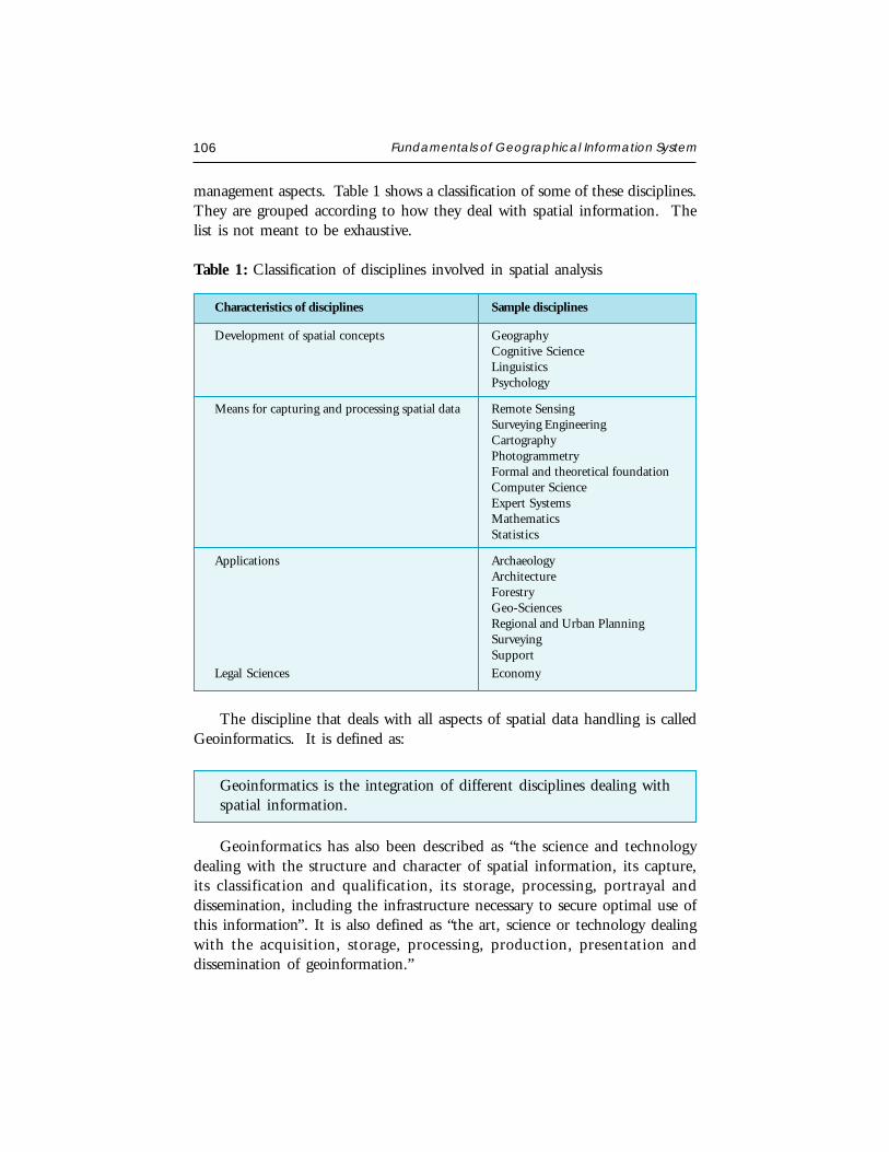
106 Fundamentals of Geographical Information System
management aspects. Table 1 shows a classification of some of these disciplines.They are grouped according to how they deal with spatial information. Thelist is not meant to be exhaustive.
Table 1: Classification of disciplines involved in spatial analysis
Characteristics of disciplines Sample disciplines
Development of spatial concepts GeographyCognitive ScienceLinguisticsPsychology
Means for capturing and processing spatial data Remote SensingSurveying EngineeringCartographyPhotogrammetryFormal and theoretical foundationComputer ScienceExpert SystemsMathematicsStatistics
Applications ArchaeologyArchitectureForestryGeo-SciencesRegional and Urban PlanningSurveyingSupport
Legal Sciences Economy
The discipline that deals with all aspects of spatial data handling is calledGeoinformatics. It is defined as:
Geoinformatics is the integration of different disciplines dealing withspatial information.
Geoinformatics has also been described as “the science and technologydealing with the structure and character of spatial information, its capture,its classification and qualification, its storage, processing, portrayal anddissemination, including the infrastructure necessary to secure optimal use ofthis information”. It is also defined as “the art, science or technology dealingwith the acquisition, storage, processing, production, presentation anddissemination of geoinformation.”

P.L.N. Raju 107
A related term that is sometimes used synonymously with geoinformaticsis Geomatics. It was originally introduced in Canada, and became very popularin French speaking countries. The term geomatics, however, was never fullyaccepted in the United States where the term geographical information scienceis preferred.
There is no clear-cut definition for GIS. Different people defined GISaccording to capability and purpose for which it is applied. Few of thedefinitions are:
“A computer - assisted system for the capture, storage, retrieval, analysisand display of spatial data, within a particular Organization” (Stillwell &Clarke, 1987).
“A powerful set of tools for collecting, storing, retrieving at will,transforming and displaying spatial data from the real world” (Burrough,1987).
A GIS is also defined as follows (Aronoff, 1989):
- A GIS is a computer-based system that provides the following foursets of capabilities to handle geo-referenced data:
- Input,
- data management (data storage and retrieval),
- manipulation and analysis, and
- Output.
“An internally referenced, automated, spatial information system”.
“A system for capturing, storing, checking, manipulating, analyzing anddisplaying data which are spatially referenced to the Earth”.
“An information technology which stores, analyses and display both spatialand non–spatial data”.
“A database system in which most of the data are spatially indexed, andupon which a set of procedures operated in order to answer queries aboutspatial entities in the database”.
108 Fundamentals of Geographical Information System
“An automated set of functions that provides professionals with advancedcapabilities for the storage, retrieval, manipulation and display ofgeographically located data”.
“A decision support system involving the integration of spatially referenceddata in a problem solving environment”.
“A system with advanced geo – modeling capabilities”.
Although the above definitions cover a wide range of subjects, the activitiesbest refer to geographical information. Some times it is also termed as SpatialInformation Systems as it deals with located data, for objects positioned inany space, not just geographical, a term for world space. Similarly, the term‘a spatial data’ is often used as a synonym for attribute data (i.e. rainfall/temperature/ soil chemical parameters/ population data etc.).
Frequently used technical terms in spatial data handling are:
• Geographic (or geographical) Information System (GIS),
• Geo-information System,
• Spatial Information System (SIS),
• Land Information System (LIS), and
• Multi-purpose Cadastre.
Geographic information systems are used by various disciplines as toolsfor spatial data handling in a geoinformatics environment.
Depending on the interest of a particular application, a GIS can beconsidered to be a data store (application of a spatial database), a tool- (box),a technology, an information source or a science (spatial information science).
Like in any other discipline, the use of tools for problem solving is onething; to produce these tools is something different. Not all are equally wellsuited for a particular application. Tools can be improved and perfected tobetter serve a particular need or application. The discipline that provides thebackground for the production of the tools in spatial data handling is spatialinformation theory (or SIT).
P.L.N. Raju 109
Geographic information technology is used to manipulate objects ingeographic space, and to acquire knowledge from spatial facts. Spatialinformation theory provides a basis for GIS by bringing together fields thatdeal with spatial reasoning, the representation of space, and humanunderstanding of space:
Spatial reasoning addresses the inference of spatial information from spatialfacts. It deals with the framework and models for space and time, and therelationships that can be identified between objects in a spatio-temporal modelof real world phenomena.
Scientific methods for the representation of space are important for thedevelopment of data models and data structures to represent objects in spatialdatabases. Spatial databases are distinguished from standard databases by theircapability to store and manage data with an extent in space and time (spatialdata types).
The human understanding of space, influenced by language and culture,plays an important role in how people design and use GIS.
The theory is used for the design of high-level models of spatial phenomenaand processes. They are then mapped into conceptual, logical and physicalmodels of spatial databases. The database stands central in the geoinformaticsenvironment. It is the database that holds the data; without it, no usefulfunction can be performed. Data are entered into the database in inputprocesses. Later, they are extracted from the database for spatial analysis anddisplay.
The processes of data management, analysis and display are often supportedby rules that are derived from domain experts. Systems that apply stored rulesto arrive at conclusions, are called rule-based or knowledge-based systems.Those that support decision making for space-related problems are known asspatial decision support systems (or SDSS). They are becoming increasinglypopular in planning agencies and management of natural resources.
All these activities happen in a social, economic and legal context. It isgenerally referred to as spatial information infrastructure. Everything withinthis infrastructure and all concepts of space and time in turn are shaped anddetermined by the cultural background of the individuals and organizationsinvolved.
110 Fundamentals of Geographical Information System
HISTORY OF GIS
The GIS history dates back to 1960 when computer based GIS have beenused and their manual procedures were in life 100 years earlier or so. Theinitial developments originated in North America with the organizations suchas US Bureau of the Census, The US Geological Survey and The HarvardLaboratory for computer graphics and Environmental Systems ResearchInstitute (commercial). Canadian Geographic Information Systems (CGIS) inCanada, Natural Experimental Research Center (NREC), Department ofEnvironment (DOE) and other notable organizations in U.K. were involvedin early developments. The laboratory for Computer Graphics and SpatialAnalysis of the Harvard Graduate School of Design and the State Universityof New York at Buffalo achieved worldwide recognition. Commercial agenciesstarted to develop and offer GIS software. Among them were today’s marketleaders ESRI, Intergraph, Laserscan, Autodesk etc.
A sound and stable data structure to store and analyze map data becamedominant in the early 1970’s. This has lead to the introduction of topologyinto GIS. Topology and the related graph theory proved to be effective andefficient tools to provide logically consistent two-dimensional datarepresentations. Another significant break through occurred with theintroduction and spread of personal computers in 1980’s. It was possible tohave a computer on the desk that was able to execute programs that previouslycould only be run on mainframe computers. At the same time minicomputers,and later, workstations became widely available. Relational database technologybecame the standard. Research on spatial data structures, indexing methods,and spatial databases made tremendous progress. The 1990’s can becharacterized as a period of the breakthrough of object-orientation in systemand database design, recognition of geoinformatics as a professional activity,and spatial information theory as the theoretical basis for GIS. Potentialityof GIS is realized in the recent past and now it has become popular amongmany users for a variety of applications.
In India the major developments have happened during the last one-decade with significant contribution coming from Department of Spaceemphasizing the GIS applications for Natural Resources Management. Notableamong them are Natural Resource Information System (NRIS), IntegratedMission for Sustainable Development (IMSD) and Bio-diversityCharacterization at National Level. IIRS is also playing a major role in GIS
P.L.N. Raju 111
through education and training programs at the National and Internationallevel. Recently the commercial organizations in India have realized theimportance of GIS for many applications like natural resource management,infrastructure development, facility management, business/market applicationsetc. and many GIS based projects according to the user organizationrequirements were developed.
GIS OBJECTIVES
• Maximize the efficiency of planning and decision making
• Provide efficient means for data distribution and handling
• Elimination of redundant data base - minimize duplication
• Capacity to integrate information from many sources
• Complex analysis/query involving geographical referenced data to generatenew information.
For any application there are five generic questions a GIS can answer:
Location - What exists at a particular location?
Condition - Identify locations where certain conditions exist.
Trends - What has changed since?
Patterns - What spatial pattern exists?
Modeling - What if ………. ?
Elements of A GIS:
The GIS has been divided into four elements. They are hardware, software,data, and liveware. Table-2 gives complete details of different elements.
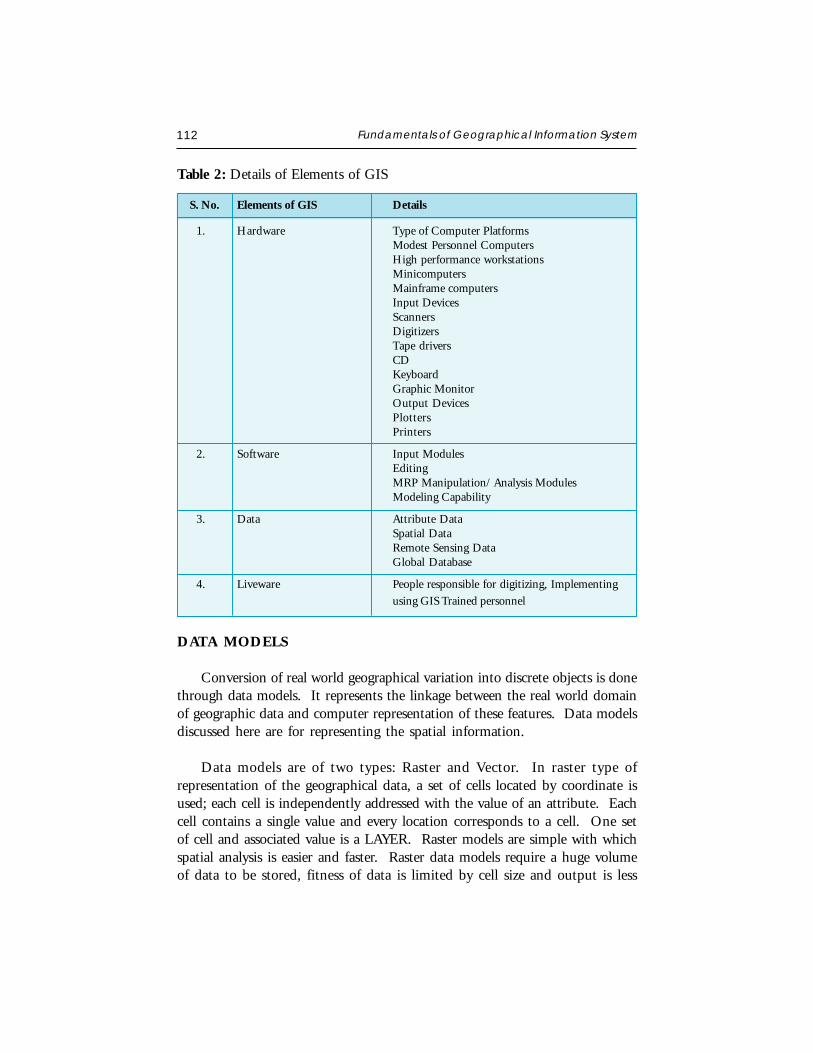
112 Fundamentals of Geographical Information System
Table 2: Details of Elements of GIS
S. No. Elements of GIS Details
1. Hardware Type of Computer PlatformsModest Personnel ComputersHigh performance workstationsMinicomputersMainframe computersInput DevicesScannersDigitizersTape driversCDKeyboardGraphic MonitorOutput DevicesPlottersPrinters
2. Software Input ModulesEditingMRP Manipulation/ Analysis ModulesModeling Capability
3. Data Attribute DataSpatial DataRemote Sensing DataGlobal Database
4. Liveware People responsible for digitizing, Implementing
using GIS Trained personnel
DATA MODELS
Conversion of real world geographical variation into discrete objects is donethrough data models. It represents the linkage between the real world domainof geographic data and computer representation of these features. Data modelsdiscussed here are for representing the spatial information.
Data models are of two types: Raster and Vector. In raster type ofrepresentation of the geographical data, a set of cells located by coordinate isused; each cell is independently addressed with the value of an attribute. Eachcell contains a single value and every location corresponds to a cell. One setof cell and associated value is a LAYER. Raster models are simple with whichspatial analysis is easier and faster. Raster data models require a huge volumeof data to be stored, fitness of data is limited by cell size and output is less
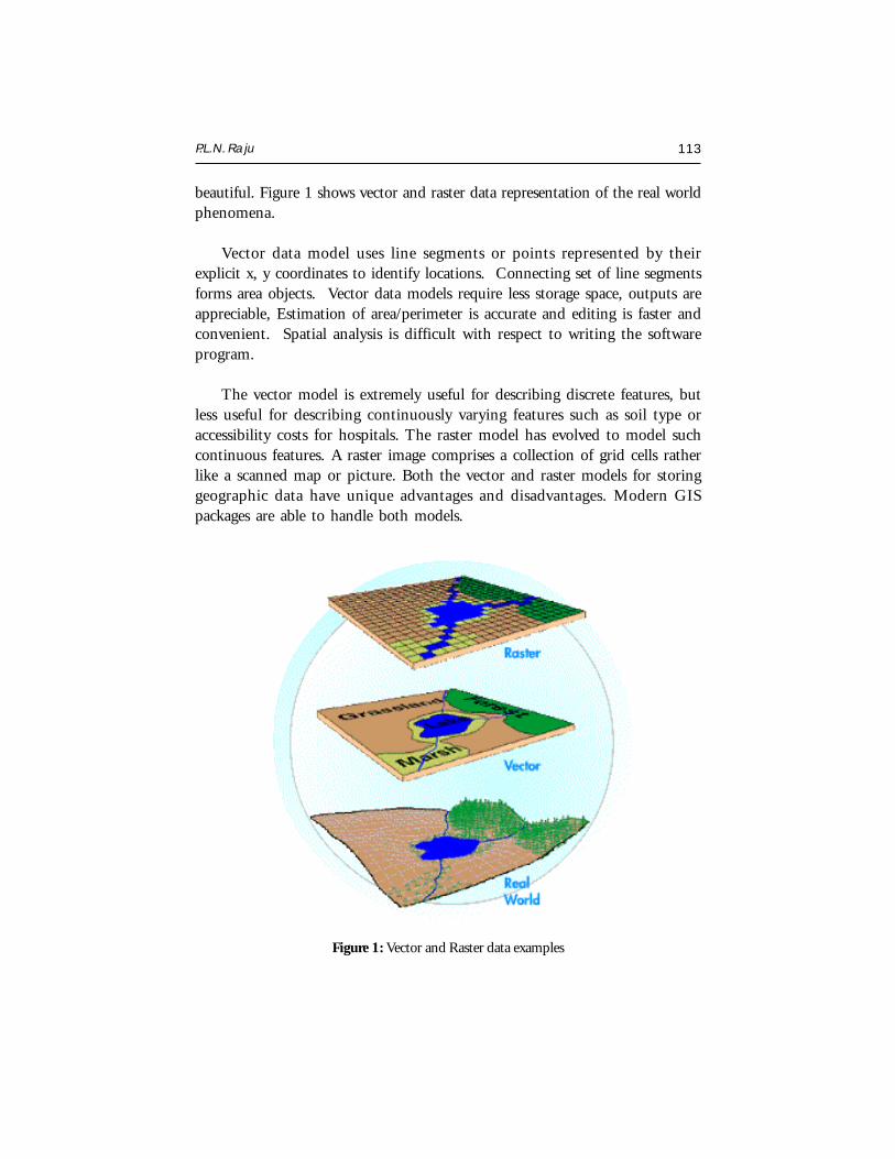
P.L.N. Raju 113
beautiful. Figure 1 shows vector and raster data representation of the real worldphenomena.
Vector data model uses line segments or points represented by theirexplicit x, y coordinates to identify locations. Connecting set of line segmentsforms area objects. Vector data models require less storage space, outputs areappreciable, Estimation of area/perimeter is accurate and editing is faster andconvenient. Spatial analysis is difficult with respect to writing the softwareprogram.
The vector model is extremely useful for describing discrete features, butless useful for describing continuously varying features such as soil type oraccessibility costs for hospitals. The raster model has evolved to model suchcontinuous features. A raster image comprises a collection of grid cells ratherlike a scanned map or picture. Both the vector and raster models for storinggeographic data have unique advantages and disadvantages. Modern GISpackages are able to handle both models.
Figure 1: Vector and Raster data examples
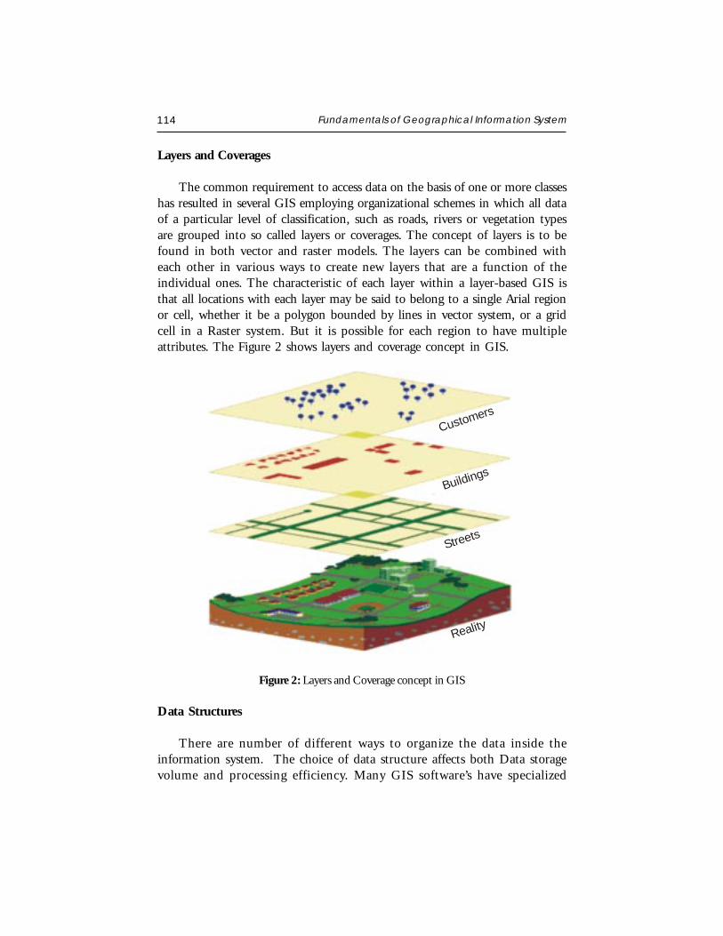
114 Fundamentals of Geographical Information System
Layers and Coverages
The common requirement to access data on the basis of one or more classeshas resulted in several GIS employing organizational schemes in which all dataof a particular level of classification, such as roads, rivers or vegetation typesare grouped into so called layers or coverages. The concept of layers is to befound in both vector and raster models. The layers can be combined witheach other in various ways to create new layers that are a function of theindividual ones. The characteristic of each layer within a layer-based GIS isthat all locations with each layer may be said to belong to a single Arial regionor cell, whether it be a polygon bounded by lines in vector system, or a gridcell in a Raster system. But it is possible for each region to have multipleattributes. The Figure 2 shows layers and coverage concept in GIS.
Figure 2: Layers and Coverage concept in GIS
Data Structures
There are number of different ways to organize the data inside theinformation system. The choice of data structure affects both Data storagevolume and processing efficiency. Many GIS software’s have specialized
Customers
Buildings
Streets
Reality
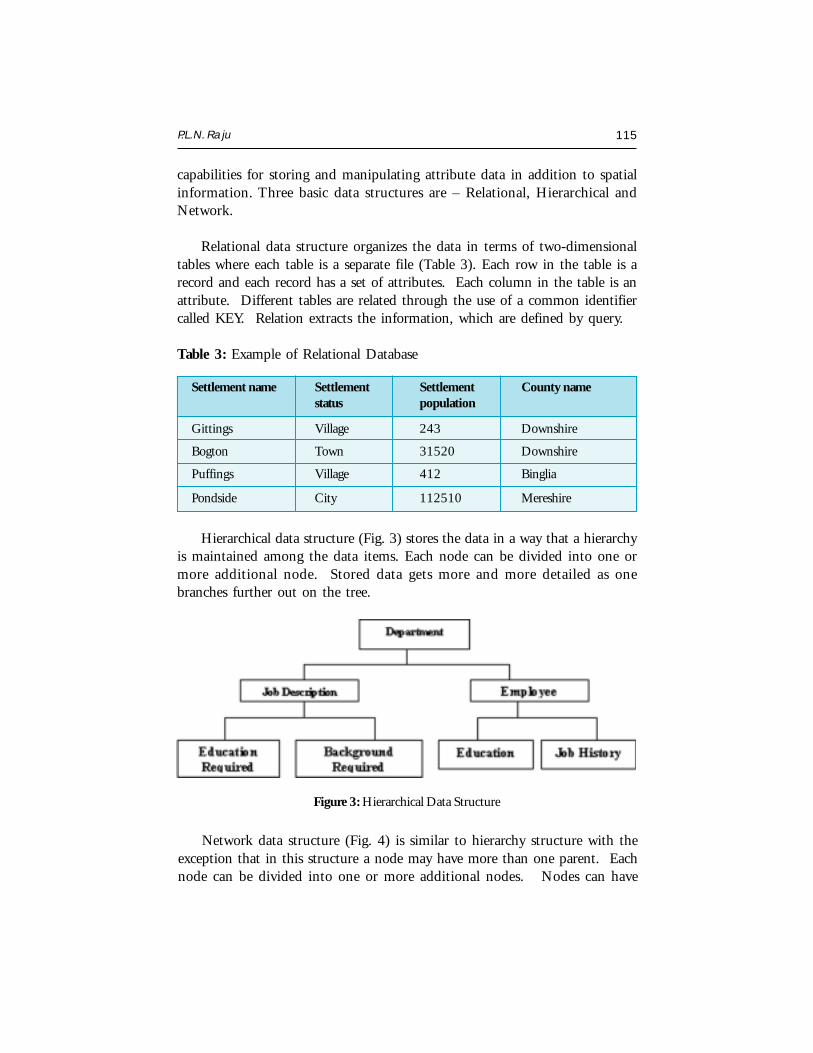
P.L.N. Raju 115
capabilities for storing and manipulating attribute data in addition to spatialinformation. Three basic data structures are – Relational, Hierarchical andNetwork.
Relational data structure organizes the data in terms of two-dimensionaltables where each table is a separate file (Table 3). Each row in the table is arecord and each record has a set of attributes. Each column in the table is anattribute. Different tables are related through the use of a common identifiercalled KEY. Relation extracts the information, which are defined by query.
Table 3: Example of Relational Database
Settlement name Settlement Settlement County namestatus population
Gittings Village 243 Downshire
Bogton Town 31520 Downshire
Puffings Village 412 Binglia
Pondside City 112510 Mereshire
Hierarchical data structure (Fig. 3) stores the data in a way that a hierarchyis maintained among the data items. Each node can be divided into one ormore additional node. Stored data gets more and more detailed as onebranches further out on the tree.
Figure 3: Hierarchical Data Structure
Network data structure (Fig. 4) is similar to hierarchy structure with theexception that in this structure a node may have more than one parent. Eachnode can be divided into one or more additional nodes. Nodes can have
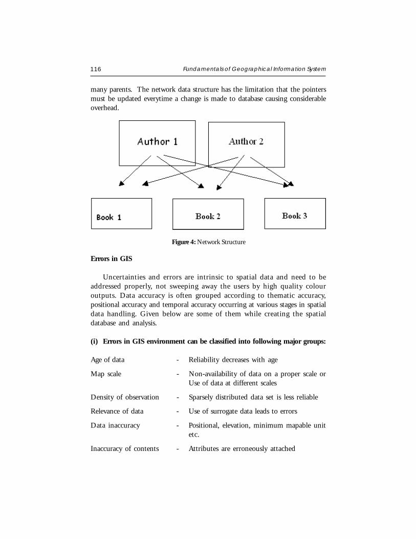
116 Fundamentals of Geographical Information System
many parents. The network data structure has the limitation that the pointersmust be updated everytime a change is made to database causing considerableoverhead.
Figure 4: Network Structure
Errors in GIS
Uncertainties and errors are intrinsic to spatial data and need to beaddressed properly, not sweeping away the users by high quality colouroutputs. Data accuracy is often grouped according to thematic accuracy,positional accuracy and temporal accuracy occurring at various stages in spatialdata handling. Given below are some of them while creating the spatialdatabase and analysis.
(i) Errors in GIS environment can be classified into following major groups:
Age of data - Reliability decreases with age
Map scale - Non-availability of data on a proper scale orUse of data at different scales
Density of observation - Sparsely distributed data set is less reliable
Relevance of data - Use of surrogate data leads to errors
Data inaccuracy - Positional, elevation, minimum mapable unitetc.
Inaccuracy of contents - Attributes are erroneously attached

P.L.N. Raju 117
(ii) Errors associated with processing :
Map digitization errors - due to boundary location problems on mapsand errors associated with digitalrepresentation of features
Rasteurization errors - due to topological mismatch arising duringapproximation by grid
Spatial Integration errors - due to map integration resulting in spuriouspolygons
Generalization errors - due to aggregation process when features areabstracted to lower scale
Attribute mismatch errors.
Misuse of Logic
The errors are also added from the source of data. Care must be taken increating spatial databases from the accurate and reliable sources of data.Realizing the importance the users may demand in future to provide themthe desired data with a tag showing how much of the data is accurate, spatialdata must be presented in quantitative terms.
Spatial Analysis
Whether it is effective utilization of natural resources or sustainabledevelopment or natural disaster management, selecting the best site for wastedisposal, optimum route alignment or local problems have a geographicalcomponent; geoinformatics will give you power to create maps, integrateinformation, visualize scenarios, solve complicated problems, present powerfulideas, and develop effective solutions like never before. In brief it can bedescribed as a supporting tool for decision-making process. Map making andgeographic analysis are not new, but a GIS performs these tasks better andfaster than do the old manual methods. Today, GIS is a multibillion-dollarindustry employing hundreds of thousands of people worldwide.
GIS is used to perform a variety of Spatial analysis, including overlayingcombinations of features and recording resultant conditions, analyzing flowsor other characteristics of networks; proximity analysis (i.e. buffet zoning) and

118 Fundamentals of Geographical Information System
defining districts in terms of spatial criteria. GIS can interrogate geographicfeatures and retrieve associated attribute information, called identification. Itcan generate new set of maps by query and analysis. It also evolves newinformation by spatial operations. Following are the analytical proceduresapplied with a GIS. GIS operational procedure and analytical tasks that areparticularly useful for spatial analysis include:
# Single layer operations
# Multi layer operations/ Topological overlay
# Geometric modeling
Calculating the distance between geographic features
Calculating area, length and perimeter
Geometric buffers.
# Network analysis
# Surface analysis
# Raster/Grid analysis
There are many applications of Geoinformatics, viz. facility management,planning, environmental monitoring, population census analysis, insuranceassessment, and health service provision, hazard mapping and many otherapplications. The following list shows few applications in natural resourcemanagement:
Agricultural development
Land evaluation analysis
Change detection of vegetated areas
Analysis of deforestation and associated environmental hazards
Monitoring vegetation health
Mapping percentage vegetation cover for the management of land
Crop acreage and production estimation
Wasteland mapping

P.L.N. Raju 119
Soil resources mapping
Groundwater potential mapping
Geological and mineral exploration
Snow-melt run-off forecasting
Monitoring forest fire
Monitoring ocean productivity etc.
GIS application in Forestry
With the rise of World Wide Web, new Internet protocols such as theHypertext Transfer Protocol (HTTP), as well as easy to use interfaces (browsers),tools and languages (HTML, XML, and Java), the Internet has become a hubfor GIS functionalities from the client side without even any GIS software.The GIS field is still evolving and it will be the major force in various walksof life dealing with geographic information.
CONCLUSIONS
Geographic Information System (GIS) is used by multi-disciplines as toolsfor spatial data handling in a geographic environment. Basic elements of GISconsist of hardware, software, data and liveware. GIS is considered one of theimportant tool for decision making in problem solving environment dealingwith geo-information.
REFERENCES
Aronoff, S. 1989. Geographic Information Systems: A Management Perspective. Ottawa,Canada : WDC Publications.
Burrough, P.A. 1987. Principles of Geographical Information Systems for Land ResourceAssessment. Oxford : Claredon Press.
Stillwell John and Clarke Graham (ed.) 1987. Applied GIS and Spatial Analysis. WestSussex : John Wiley and Sons, 2004.
http://www.ncgia.ucsb.edu/~spalladi/thesis/Chapter3.html
http://www.sli.unimelb.edu.au/gisweb/menu.html
http://www.gislinx.com/Software/Programs/MicroStation/index.shtml

120 Fundamentals of Geographical Information System
http://geog.hkbu.edu.hk/geog3600/ (Hongkong Baptist University)
http://geosun.sjsu.edu/paula/137/ppt/lecture13/sld008.htm
http://www.ccrs.nrcan.gc.ca/ccrs/eduref/tutorial/tutore.html
http://www.cla.sc.edu/gis/avshtcrs/handouts.html
http://www.gisdevelopment.net
http://www.planweb.co.uk/
http://www.sbg.ac.at/geo/idrisi/wwwtutor/tuthome.htm
http://www.ed.ac.uk/
http://www.geoplace.com
FUNDAMENTALS OF GPS
P.L.N. RajuGeoinformatics DivisionIndian Institute of Remote Sensing, Dehra Dun
Abstract : Conventional methods of surveying and navigation require tedious fieldand astronomical observations for deriving positional and directional information.Rapid advancement in higher frequency signal transmission and precise clock signalsalong with advanced satellite technology have led to the development of GlobalPositioning System (GPS). The outcome of a typical GPS survey includes geocentricposition accurate to 10 m and relative positions between receiver locations tocentimeter level or better. Technological aspect as well as applications of GPS in
various fields are discussed in this paper.
INTRODUCTION
Traditional methods of surveying and navigation resort to tedious fieldand astronomical observation for deriving positional and directionalinformation. Diverse field conditions, seasonal variation and many unavoidablecircumstances always bias the traditional field approach. However, due to rapidadvancement in electronic systems, every aspect of human life is affected to agreat deal. Field of surveying and navigation is tremendously benefited throughelectronic devices. Many of the critical situations in surveying/navigation arenow easily and precisely solved in short time.
Astronomical observation of celestial bodies was one of the standardmethods of obtaining coordinates of a position. This method is prone tovisibility and weather condition and demands expert handling. Attempts havebeen made by USA since early 1960’s to use space based artificial satellites.System TRANSIT was widely used for establishing a network of control pointsover large regions. Establishment of modern geocentric datum and its relationto local datum was successfully achieved through TRANSIT. Rapidimprovements in higher frequently transmission and precise clock signals along
Satellite Remote Sensing and GIS Applications in Agricultural Meteorologypp. 121-150
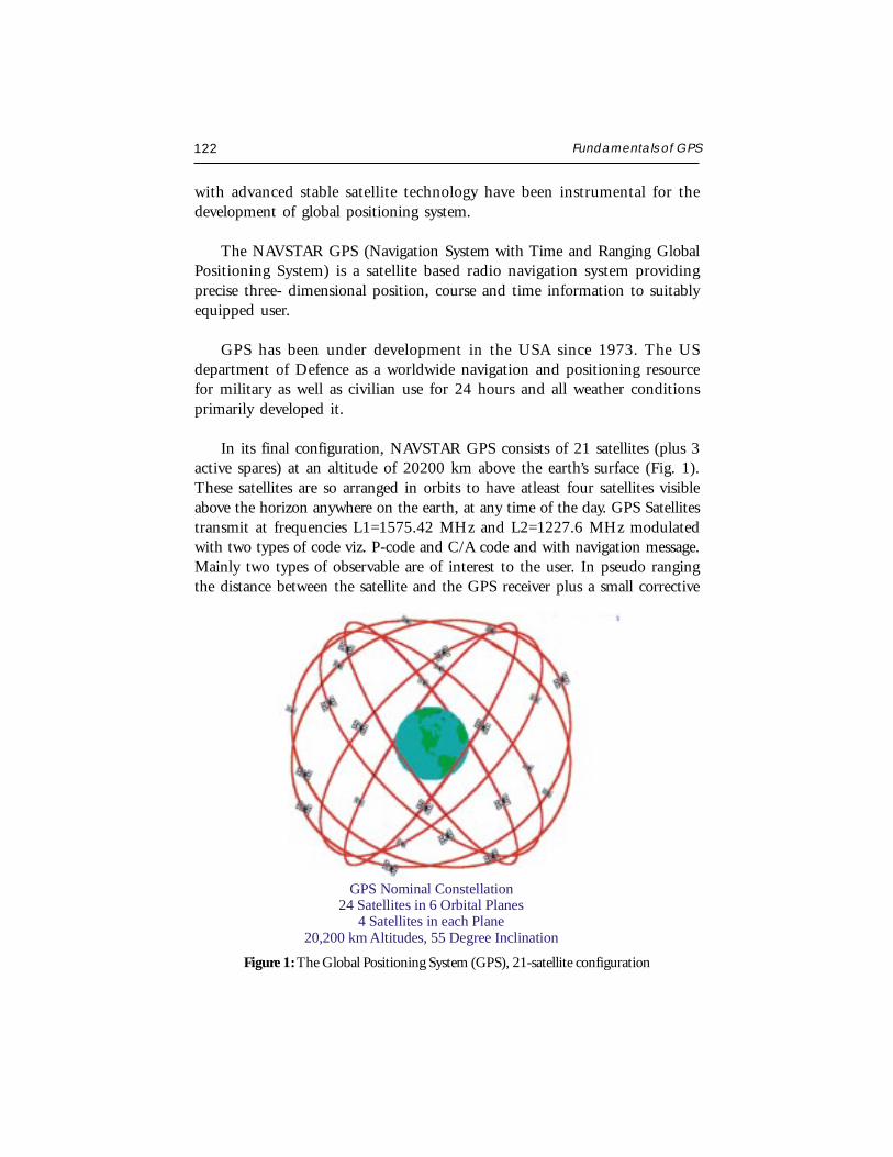
122 Fundamentals of GPS
with advanced stable satellite technology have been instrumental for thedevelopment of global positioning system.
The NAVSTAR GPS (Navigation System with Time and Ranging GlobalPositioning System) is a satellite based radio navigation system providingprecise three- dimensional position, course and time information to suitablyequipped user.
GPS has been under development in the USA since 1973. The USdepartment of Defence as a worldwide navigation and positioning resourcefor military as well as civilian use for 24 hours and all weather conditionsprimarily developed it.
In its final configuration, NAVSTAR GPS consists of 21 satellites (plus 3active spares) at an altitude of 20200 km above the earth’s surface (Fig. 1).These satellites are so arranged in orbits to have atleast four satellites visibleabove the horizon anywhere on the earth, at any time of the day. GPS Satellitestransmit at frequencies L1=1575.42 MHz and L2=1227.6 MHz modulatedwith two types of code viz. P-code and C/A code and with navigation message.Mainly two types of observable are of interest to the user. In pseudo rangingthe distance between the satellite and the GPS receiver plus a small corrective
Figure 1: The Global Positioning System (GPS), 21-satellite configuration
GPS Nominal Constellation24 Satellites in 6 Orbital Planes
4 Satellites in each Plane20,200 km Altitudes, 55 Degree Inclination
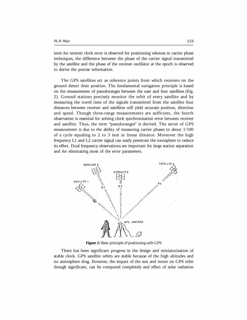
P.L.N. Raju 123
term for receiver clock error is observed for positioning whereas in carrier phasetechniques, the difference between the phase of the carrier signal transmittedby the satellite and the phase of the receiver oscillator at the epoch is observedto derive the precise information.
The GPS satellites act as reference points from which receivers on theground detect their position. The fundamental navigation principle is basedon the measurement of pseudoranges between the user and four satellites (Fig.2). Ground stations precisely monitor the orbit of every satellite and bymeasuring the travel time of the signals transmitted from the satellite fourdistances between receiver and satellites will yield accurate position, directionand speed. Though three-range measurements are sufficient, the fourthobservation is essential for solving clock synchronization error between receiverand satellite. Thus, the term “pseudoranges” is derived. The secret of GPSmeasurement is due to the ability of measuring carrier phases to about 1/100of a cycle equaling to 2 to 3 mm in linear distance. Moreover the highfrequency L1 and L2 carrier signal can easily penetrate the ionosphere to reduceits effect. Dual frequency observations are important for large station separationand for eliminating most of the error parameters.
Figure 2: Basic principle of positioning with GPS
There has been significant progress in the design and miniaturization ofstable clock. GPS satellite orbits are stable because of the high altitudes andno atmosphere drag. However, the impact of the sun and moon on GPS orbitthough significant, can be computed completely and effect of solar radiation
R1
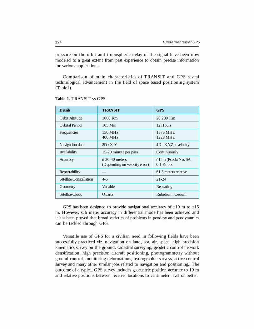
124 Fundamentals of GPS
pressure on the orbit and tropospheric delay of the signal have been nowmodeled to a great extent from past experience to obtain precise informationfor various applications.
Comparison of main characteristics of TRANSIT and GPS revealtechnological advancement in the field of space based positioning system(Table1).
Table 1. TRANSIT vs GPS
Details TRANSIT GPS
Orbit Altitude 1000 Km 20,200 Km
Orbital Period 105 Min 12 Hours
Frequencies 150 MHz 1575 MHz400 MHz 1228 MHz
Navigation data 2D : X, Y 4D : X,Y,Z, t velocity
Availability 15-20 minute per pass Continuously
Accuracy ñ 30-40 meters ñ15m (Pcode/No. SA(Depending on velocity error) 0.1 Knots
Repeatability — ñ1.3 meters relative
Satellite Constellation 4-6 21-24
Geometry Variable Repeating
Satellite Clock Quartz Rubidium, Cesium
GPS has been designed to provide navigational accuracy of ±10 m to ±15m. However, sub meter accuracy in differential mode has been achieved andit has been proved that broad varieties of problems in geodesy and geodynamicscan be tackled through GPS.
Versatile use of GPS for a civilian need in following fields have beensuccessfully practiced viz. navigation on land, sea, air, space, high precisionkinematics survey on the ground, cadastral surveying, geodetic control networkdensification, high precision aircraft positioning, photogrammetry withoutground control, monitoring deformations, hydrographic surveys, active controlsurvey and many other similar jobs related to navigation and positioning,. Theoutcome of a typical GPS survey includes geocentric position accurate to 10 mand relative positions between receiver locations to centimeter level or better.
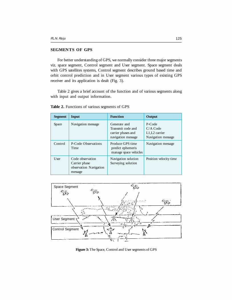
P.L.N. Raju 125
SEGMENTS OF GPS
For better understanding of GPS, we normally consider three major segmentsviz. space segment, Control segment and User segment. Space segment dealswith GPS satellites systems, Control segment describes ground based time andorbit control prediction and in User segment various types of existing GPSreceiver and its application is dealt (Fig. 3).
Table 2 gives a brief account of the function and of various segments alongwith input and output information.
Table 2. Functions of various segments of GPS
Segment Input Function Output
Space Navigation message Generate and P-CodeTransmit code and C/A Codecarrier phases and L1,L2 carriernavigation message Navigation message
Control P-Code Observations Produce GPS time Navigation messageTime predict ephemeris
manage space vehicles
User Code observation Navigation solution Position velocity timeCarrier phase Surveying solutionobservation Navigationmessage
Figure 3: The Space, Control and User segments of GPS
Control Segment
User Segment
Space Segment
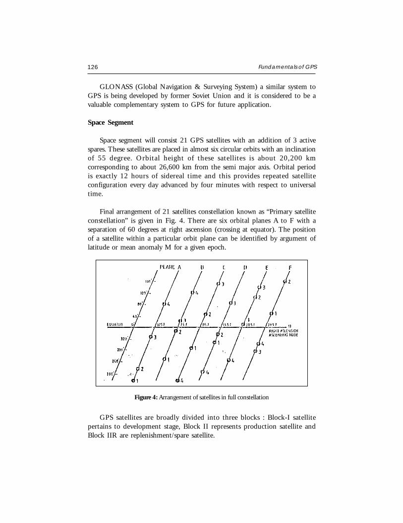
126 Fundamentals of GPS
GLONASS (Global Navigation & Surveying System) a similar system toGPS is being developed by former Soviet Union and it is considered to be avaluable complementary system to GPS for future application.
Space Segment
Space segment will consist 21 GPS satellites with an addition of 3 activespares. These satellites are placed in almost six circular orbits with an inclinationof 55 degree. Orbital height of these satellites is about 20,200 kmcorresponding to about 26,600 km from the semi major axis. Orbital periodis exactly 12 hours of sidereal time and this provides repeated satelliteconfiguration every day advanced by four minutes with respect to universaltime.
Final arrangement of 21 satellites constellation known as “Primary satelliteconstellation” is given in Fig. 4. There are six orbital planes A to F with aseparation of 60 degrees at right ascension (crossing at equator). The positionof a satellite within a particular orbit plane can be identified by argument oflatitude or mean anomaly M for a given epoch.
Figure 4: Arrangement of satellites in full constellation
GPS satellites are broadly divided into three blocks : Block-I satellitepertains to development stage, Block II represents production satellite andBlock IIR are replenishment/spare satellite.
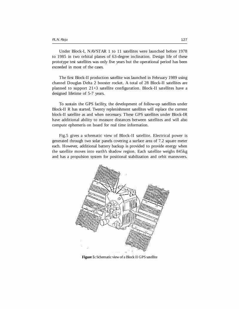
P.L.N. Raju 127
Under Block-I, NAVSTAR 1 to 11 satellites were launched before 1978to 1985 in two orbital planes of 63-degree inclination. Design life of theseprototype test satellites was only five years but the operational period has beenexceeded in most of the cases.
The first Block-II production satellite was launched in February 1989 usingchannel Douglas Delta 2 booster rocket. A total of 28 Block-II satellites areplanned to support 21+3 satellite configuration. Block-II satellites have adesigned lifetime of 5-7 years.
To sustain the GPS facility, the development of follow-up satellites underBlock-II R has started. Twenty replenishment satellites will replace the currentblock-II satellite as and when necessary. These GPS satellites under Block-IRhave additional ability to measure distances between satellites and will alsocompute ephemeris on board for real time information.
Fig.5 gives a schematic view of Block-II satellite. Electrical power isgenerated through two solar panels covering a surface area of 7.2 square metereach. However, additional battery backup is provided to provide energy whenthe satellite moves into earth’s shadow region. Each satellite weighs 845kgand has a propulsion system for positional stabilization and orbit maneuvers.
Figure 5: Schematic view of a Block II GPS satellite
128 Fundamentals of GPS
GPS satellites have a very high performance frequency standard with anaccuracy of between 1X10-12 to 1X10-13 and are thus capable of creating precisetime base. Block-I satellites were partly equipped with only quartz oscillatorsbut Block-II satellites have two cesium frequency standards and two rubidiumfrequency standards. Using fundamental frequency of 10.23 MHz, two carrierfrequencies are generated to transmit signal codes.
Observation Principle and Signal Structure
NAVSTAR GPS is a one-way ranging system i.e. signals are onlytransmitted by the satellite. Signal travel time between the satellite and thereceiver is observed and the range distance is calculated through the knowledgeof signal propagation velocity. One way ranging means that a clock readingat the transmitted antenna is compared with a clock reading at the receiverantenna. But since the two clocks are not strictly synchronized, the observedsignal travel time is biased with systematic synchronization error. Biased rangesare known as pseudoranges. Simultaneous observations of four pseudorangesare necessary to determine X, Y, Z coordinates of user antenna and clock bias.
Real time positioning through GPS signals is possible by modulatingcarrier frequency with Pseudorandom Noise (PRN) codes. These are sequenceof binary values (zeros and ones or +1 and -1) having random character butidentifiable distinctly. Thus pseudoranges are derived from travel time of anidentified PRN signal code. Two different codes viz. P-code and C/A code arein use. P means precision or protected and C/A means clear/acquisition orcoarse acquisition.
P- code has a frequency of 10.23 MHz. This refers to a sequence of 10.23million binary digits or chips per second. This frequency is also referred to asthe chipping rate of P-code. Wavelength corresponding to one chip is 29.30m.The P-code sequence is extremely long and repeats only after 266 days.Portions of seven days each are assigned to the various satellites. As aconsequence, all satellite can transmit on the same frequency and can beidentified by their unique one-week segment. This technique is also called asCode Division Multiple Access (CDMA). P-code is the primary code fornavigation and is available on carrier frequencies L1 and L2.
The C/A code has a length of only one millisecond; its chipping rate is1.023 MHz with corresponding wavelength of 300 meters. C/A code is onlytransmitted on L1 carrier.
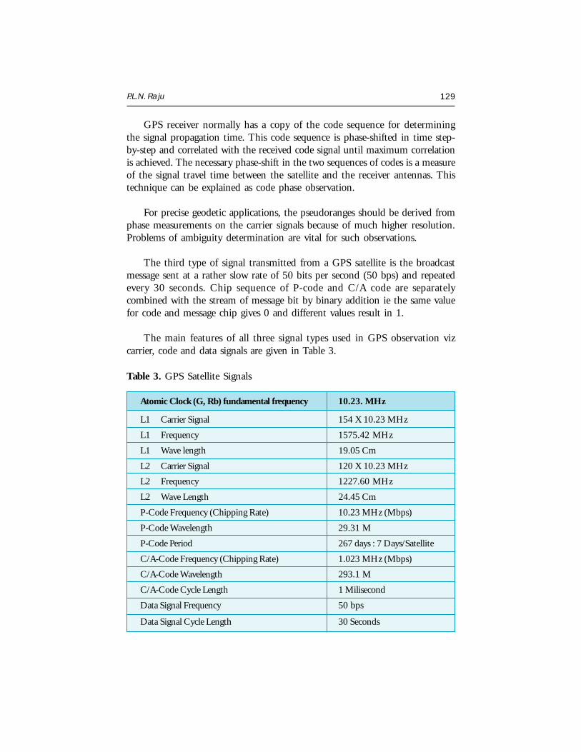
P.L.N. Raju 129
GPS receiver normally has a copy of the code sequence for determiningthe signal propagation time. This code sequence is phase-shifted in time step-by-step and correlated with the received code signal until maximum correlationis achieved. The necessary phase-shift in the two sequences of codes is a measureof the signal travel time between the satellite and the receiver antennas. Thistechnique can be explained as code phase observation.
For precise geodetic applications, the pseudoranges should be derived fromphase measurements on the carrier signals because of much higher resolution.Problems of ambiguity determination are vital for such observations.
The third type of signal transmitted from a GPS satellite is the broadcastmessage sent at a rather slow rate of 50 bits per second (50 bps) and repeatedevery 30 seconds. Chip sequence of P-code and C/A code are separatelycombined with the stream of message bit by binary addition ie the same valuefor code and message chip gives 0 and different values result in 1.
The main features of all three signal types used in GPS observation vizcarrier, code and data signals are given in Table 3.
Table 3. GPS Satellite Signals
Atomic Clock (G, Rb) fundamental frequency 10.23. MHz
L1 Carrier Signal 154 X 10.23 MHz
L1 Frequency 1575.42 MHz
L1 Wave length 19.05 Cm
L2 Carrier Signal 120 X 10.23 MHz
L2 Frequency 1227.60 MHz
L2 Wave Length 24.45 Cm
P-Code Frequency (Chipping Rate) 10.23 MHz (Mbps)
P-Code Wavelength 29.31 M
P-Code Period 267 days : 7 Days/Satellite
C/A-Code Frequency (Chipping Rate) 1.023 MHz (Mbps)
C/A-Code Wavelength 293.1 M
C/A-Code Cycle Length 1 Milisecond
Data Signal Frequency 50 bps
Data Signal Cycle Length 30 Seconds
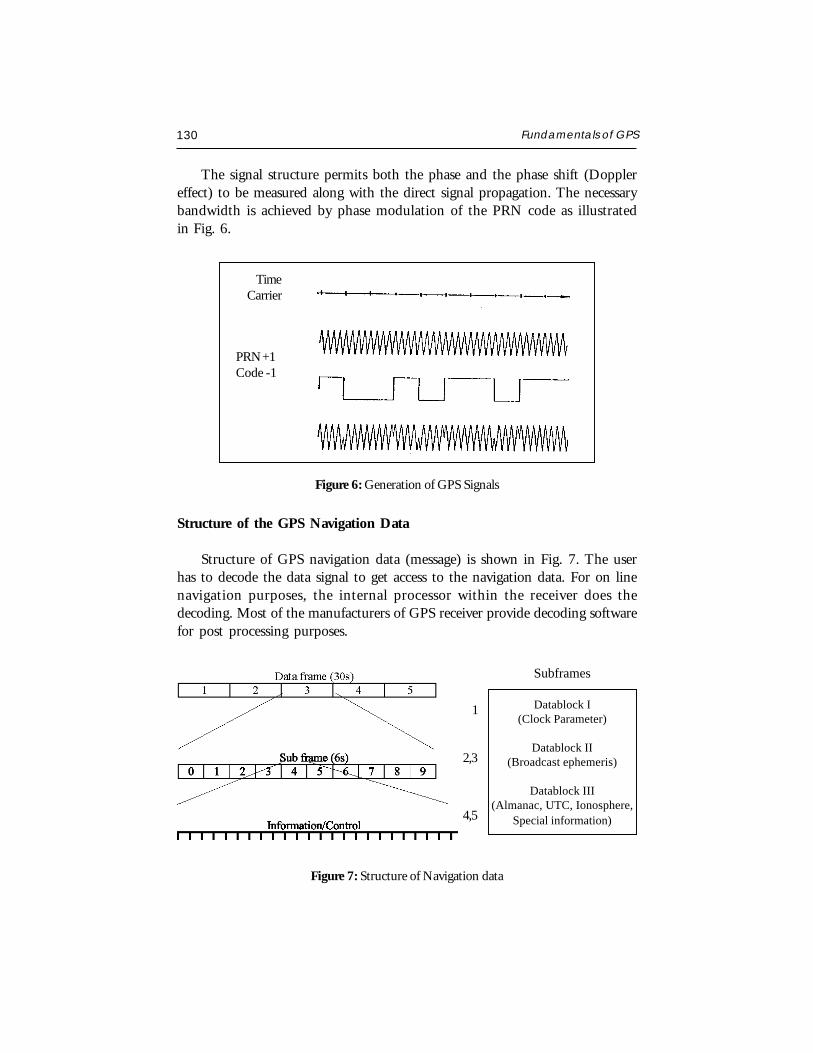
130 Fundamentals of GPS
The signal structure permits both the phase and the phase shift (Dopplereffect) to be measured along with the direct signal propagation. The necessarybandwidth is achieved by phase modulation of the PRN code as illustratedin Fig. 6.
PRN +1Code -1
TimeCarrier
Figure 6: Generation of GPS Signals
Structure of the GPS Navigation Data
Structure of GPS navigation data (message) is shown in Fig. 7. The userhas to decode the data signal to get access to the navigation data. For on linenavigation purposes, the internal processor within the receiver does thedecoding. Most of the manufacturers of GPS receiver provide decoding softwarefor post processing purposes.
Subframes
Datablock I(Clock Parameter)
Datablock II(Broadcast ephemeris)
Datablock III(Almanac, UTC, Ionosphere,
Special information)
1
2,3
4,5
Figure 7: Structure of Navigation data
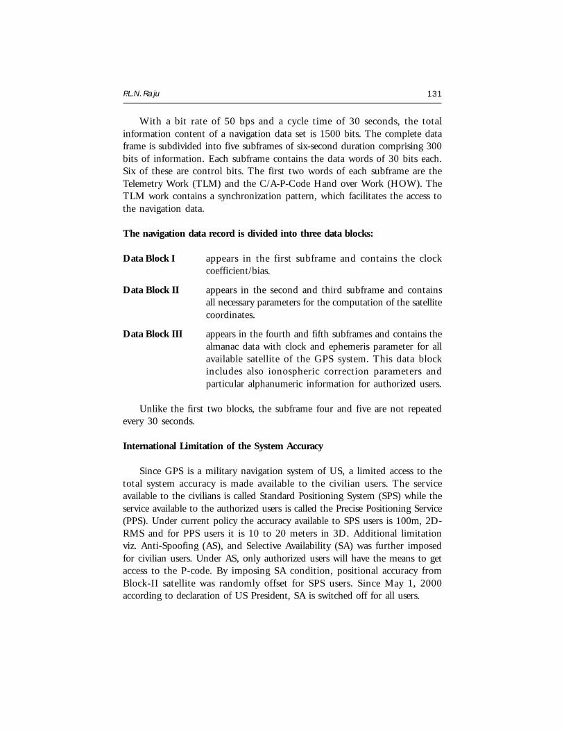
P.L.N. Raju 131
With a bit rate of 50 bps and a cycle time of 30 seconds, the totalinformation content of a navigation data set is 1500 bits. The complete dataframe is subdivided into five subframes of six-second duration comprising 300bits of information. Each subframe contains the data words of 30 bits each.Six of these are control bits. The first two words of each subframe are theTelemetry Work (TLM) and the C/A-P-Code Hand over Work (HOW). TheTLM work contains a synchronization pattern, which facilitates the access tothe navigation data.
The navigation data record is divided into three data blocks:
Data Block I appears in the first subframe and contains the clockcoefficient/bias.
Data Block II appears in the second and third subframe and containsall necessary parameters for the computation of the satellitecoordinates.
Data Block III appears in the fourth and fifth subframes and contains thealmanac data with clock and ephemeris parameter for allavailable satellite of the GPS system. This data blockincludes also ionospheric correction parameters andparticular alphanumeric information for authorized users.
Unlike the first two blocks, the subframe four and five are not repeatedevery 30 seconds.
International Limitation of the System Accuracy
Since GPS is a military navigation system of US, a limited access to thetotal system accuracy is made available to the civilian users. The serviceavailable to the civilians is called Standard Positioning System (SPS) while theservice available to the authorized users is called the Precise Positioning Service(PPS). Under current policy the accuracy available to SPS users is 100m, 2D-RMS and for PPS users it is 10 to 20 meters in 3D. Additional limitationviz. Anti-Spoofing (AS), and Selective Availability (SA) was further imposedfor civilian users. Under AS, only authorized users will have the means to getaccess to the P-code. By imposing SA condition, positional accuracy fromBlock-II satellite was randomly offset for SPS users. Since May 1, 2000according to declaration of US President, SA is switched off for all users.
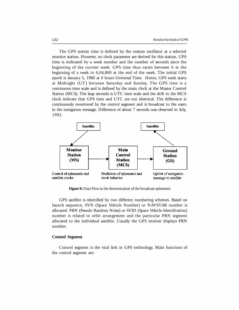
132 Fundamentals of GPS
The GPS system time is defined by the cesium oscillator at a selectedmonitor station. However, no clock parameter are derived for this station. GPStime is indicated by a week number and the number of seconds since thebeginning of the current week. GPS time thus varies between 0 at thebeginning of a week to 6,04,800 at the end of the week. The initial GPSepoch is January 5, 1980 at 0 hours Universal Time. Hence, GPS week startsat Midnight (UT) between Saturday and Sunday. The GPS time is acontinuous time scale and is defined by the main clock at the Master ControlStation (MCS). The leap seconds is UTC time scale and the drift in the MCSclock indicate that GPS time and UTC are not identical. The difference iscontinuously monitored by the control segment and is broadcast to the usersin the navigation message. Difference of about 7 seconds was observed in July,1992.
Figure 8: Data Flow in the determination of the broadcast ephemeris
GPS satellite is identified by two different numbering schemes. Based onlaunch sequence, SVN (Space Vehicle Number) or NAVSTAR number isallocated. PRN (Pseudo Random Noise) or SVID (Space Vehicle Identification)number is related to orbit arrangement and the particular PRN segmentallocated to the individual satellite. Usually the GPS receiver displays PRNnumber.
Control Segment
Control segment is the vital link in GPS technology. Main functions ofthe control segment are:
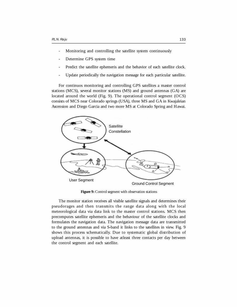
P.L.N. Raju 133
- Monitoring and controlling the satellite system continuously
- Determine GPS system time
- Predict the satellite ephemeris and the behavior of each satellite clock.
- Update periodically the navigation message for each particular satellite.
For continuos monitoring and controlling GPS satellites a master controlstations (MCS), several monitor stations (MS) and ground antennas (GA) arelocated around the world (Fig. 9). The operational control segment (OCS)consists of MCS near Colorado springs (USA), three MS and GA in KwajaleianAscension and Diego Garcia and two more MS at Colorado Spring and Hawai.
Figure 9: Control segment with observation stations
The monitor station receives all visible satellite signals and determines theirpseudorages and then transmits the range data along with the localmeteorological data via data link to the master control stations. MCS thenprecomputes satellite ephemeris and the behaviour of the satellite clocks andformulates the navigation data. The navigation message data are transmittedto the ground antennas and via S-band it links to the satellites in view. Fig. 9shows this process schematically. Due to systematic global distribution ofupload antennas, it is possible to have atleast three contacts per day betweenthe control segment and each satellite.
SatelliteConstellation
User SegmentGround Control Segment
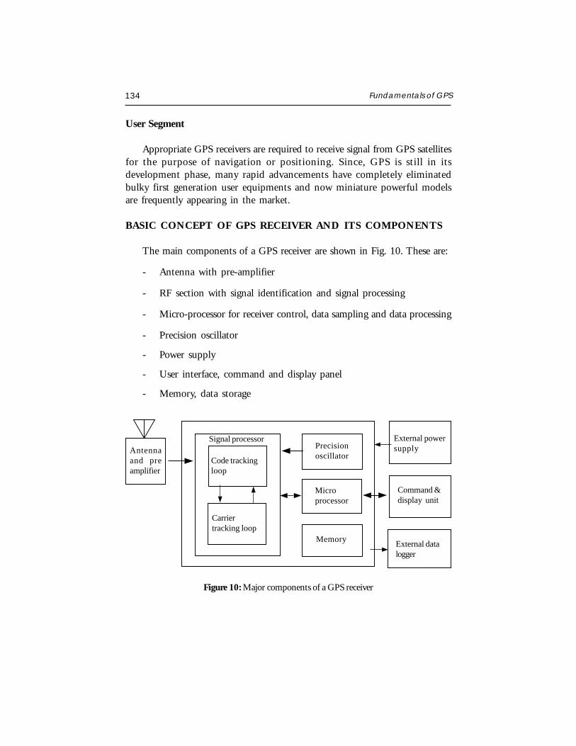
134 Fundamentals of GPS
User Segment
Appropriate GPS receivers are required to receive signal from GPS satellitesfor the purpose of navigation or positioning. Since, GPS is still in itsdevelopment phase, many rapid advancements have completely eliminatedbulky first generation user equipments and now miniature powerful modelsare frequently appearing in the market.
BASIC CONCEPT OF GPS RECEIVER AND ITS COMPONENTS
The main components of a GPS receiver are shown in Fig. 10. These are:
- Antenna with pre-amplifier
- RF section with signal identification and signal processing
- Micro-processor for receiver control, data sampling and data processing
- Precision oscillator
- Power supply
- User interface, command and display panel
- Memory, data storage
Code trackingloop
Carriertracking loop
Precisionoscillator
Microprocessor
Memory
External powersupply
Command &display unit
External datalogger
Antennaand preamplifier
Signal processor
Figure 10: Major components of a GPS receiver
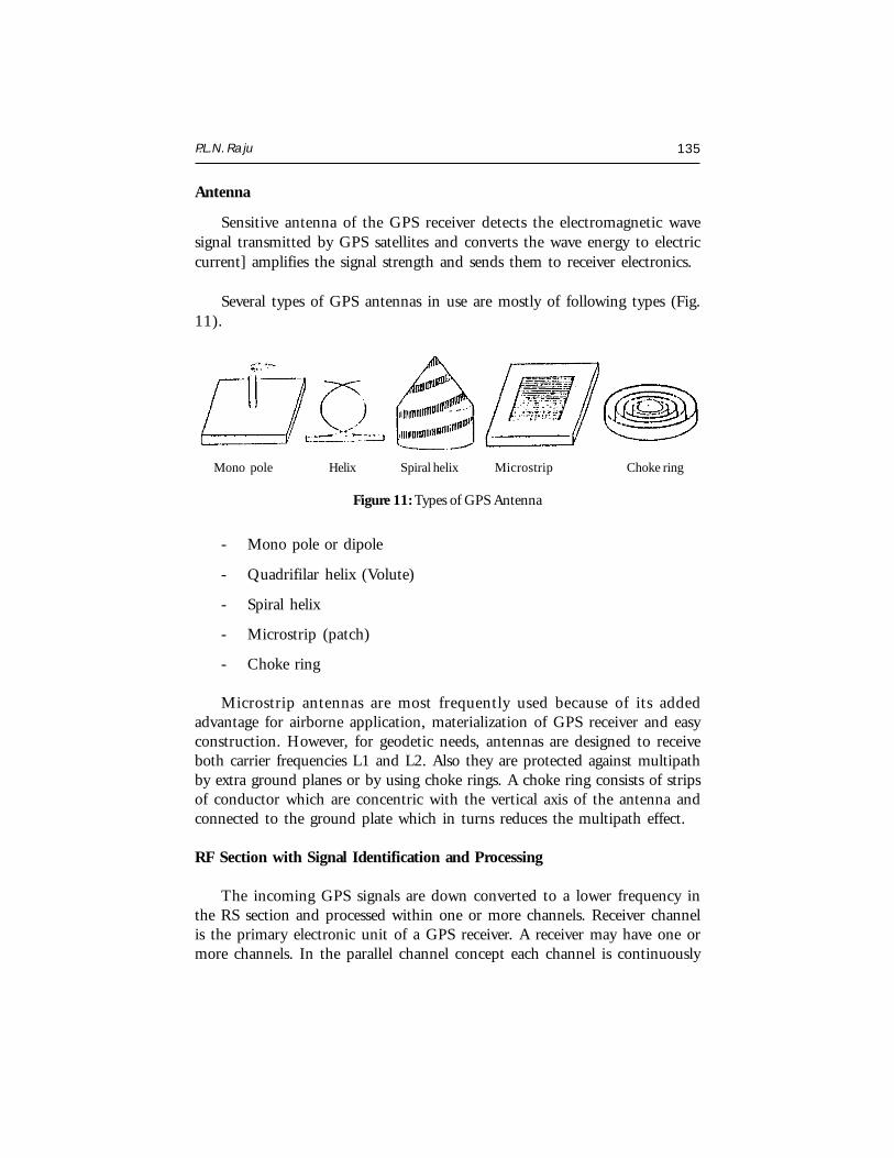
P.L.N. Raju 135
Antenna
Sensitive antenna of the GPS receiver detects the electromagnetic wavesignal transmitted by GPS satellites and converts the wave energy to electriccurrent] amplifies the signal strength and sends them to receiver electronics.
Several types of GPS antennas in use are mostly of following types (Fig.11).
Mono pole Helix Spiral helix Microstrip Choke ring
Figure 11: Types of GPS Antenna
- Mono pole or dipole
- Quadrifilar helix (Volute)
- Spiral helix
- Microstrip (patch)
- Choke ring
Microstrip antennas are most frequently used because of its addedadvantage for airborne application, materialization of GPS receiver and easyconstruction. However, for geodetic needs, antennas are designed to receiveboth carrier frequencies L1 and L2. Also they are protected against multipathby extra ground planes or by using choke rings. A choke ring consists of stripsof conductor which are concentric with the vertical axis of the antenna andconnected to the ground plate which in turns reduces the multipath effect.
RF Section with Signal Identification and Processing
The incoming GPS signals are down converted to a lower frequency inthe RS section and processed within one or more channels. Receiver channelis the primary electronic unit of a GPS receiver. A receiver may have one ormore channels. In the parallel channel concept each channel is continuously
136 Fundamentals of GPS
franking one particular satellite. A minimum of four parallel channels isrequired to determine position and time. Modern receivers contain upto 12channels for each frequency.
In the sequencing channel concept the channel switches from satellite tosatellite at regular interval. A single channel receiver takes atleast four timesof 30 seconds to establish first position fix, though some receiver types have adedicated channel for reading the data signal. Now days in most of the casesfast sequencing channels with a switching rate of about one-second per satelliteare used.
In multiplexing channel, sequencing at a very high speed between differentsatellites is achieved using one or both frequencies. The switching rate issynchronous with the navigation message of 50 bps or 20 milliseconds perbit. A complete sequence with four satellites is completed by 20 millisecondor after 40 millisecond for dual frequency receivers. The navigation messageis continuous, hence first fix is achieved after about 30 seconds.
Though continuous tracking parallel channels are cheap and give goodoverall performance, GPS receivers based on multiplexing technology will soonbe available at a cheaper price due to electronic boom.
Microprocessor
To control the operation of a GPS receiver, a microprocessor is essentialfor acquiring the signals, processing of the signal and the decoding of thebroadcast message. Additional capabilities of computation of on-line positionand velocity, conversion into a given local datum or the determination ofwaypoint information are also required. In future more and more user relevantsoftware will be resident on miniaturized memory chips.
Precision Oscillator
A reference frequency in the receiver is generated by the precision oscillator.Normally, less expensive, low performance quartz oscillator is used in receiverssince the precise clock information is obtained from the GPS satellites andthe user clock error can be eliminated through double differencing techniquewhen all participating receivers observe at exactly the same epoch. Fornavigation with two or three satellites only an external high precision oscillatoris used.
P.L.N. Raju 137
Power Supply
First generation GPS receivers consumed very high power, but modernreceivers are designed to consume as little energy as possible. Most receivershave an internal rechargeable Nickel-Cadmium battery in addition to anexternal power input. Caution of low battery signal prompts the user to ensureadequate arrangement of power supply.
Memory Capacity
For port processing purposes all data have to be stored on internal orexternal memory devices. Post processing is essential for multi station techniquesapplicable to geodatic and surveying problems. GPS observation forpseudoranges, phase data, time and navigation message data have to berecorded. Based on sampling rate, it amount to about 1.5 Mbytes of data perhour for six satellites and 1 second data for dual frequency receivers. Modernreceivers have internal memories of 5 Mbytes or more. Some receivers storethe data on magnetic tape or on a floppy disk or hard-disk using externalmicrocomputer connected through RS-232 port.
Most modern receivers have a keypad and a display for communicationbetween the user and the receivers. The keypad is used to enter commands,external data like station number or antenna height or to select a menuoperation. The display indicates computed coordinates, visible satellites, dataquality indices and other suitable information. Current operation softwarepackages are menu driven and very user friendly.
Classification of GPS Receivers
GPS receivers can be divided into various groups according to differentcriteria. In the early stages two basic technologies were used as the classificationcriteria viz. Code correlation receiver technology and sequencing receivertechnology, which were equivalent to code dependent receivers and code freereceivers. However, this kind of division is no longer justifiable since bothtechniques are implemented in present receivers.
Another classification of GPS receivers is based on acquisition of data typese.g.
138 Fundamentals of GPS
- C/A code receiver
- C/A code + L1 Carrier phase
- C/A code + L1 Carrier phase + L2 Carrier phase
- C/A code + p_code + L1, L2 Carrier phase
- L1 Carrier phase (not very common)
- L1, L2 Carrier phase (rarely used)
Based on technical realization of channel, the GPS receivers can be classifiedas:
- Multi-channel receiver
- Sequential receiver
- Multiplexing receiver
GPS receivers are even classified on the purpose as :
- Military receiver
- Civilian receiver
- Navigation receiver
- Timing receiver
- Geodetic receiver
For geodetic application it is essential to use the carrier phase data asobservable. Use of L1 and L2 frequency is also essential along with P-code.
Examples of GPS Receiver
GPS receiver market is developing and expanding at a very high speed.Receivers are becoming powerful, cheap and smaller in size. It is not possibleto give details of every make but description of some typical receivers givenmay be regarded as a basis for the evaluation of future search and study ofGPS receivers.
Classical Receivers
Detailed description of code dependent T1 4100 GPS Navigator and codefree Macrometer V1000 is given here:
P.L.N. Raju 139
T1 4100 GPS Navigator was manufactured by Texas Instrument in 1984.It was the first GPS receiver to provide C/A and P code and L1 and L2 carrierphase observations. It is a dual frequency multiplexing receiver and suitablefor geodesist, surveyor and navigators. The observables through it are:
- P-Code pseudo ranges on L1 and L2
- C/A-Code pseudo ranges on L1
- Carrier phase on L1 and L2
The data are recorded by an external tape recorder on digital cassettes orare downloaded directly to an external microprocessor. A hand held controldisplay unit (CDU) is used for communication between observer and thereceiver. For navigational purposes the built in microprocessor provides positionand velocity in real time every three seconds. T1 4100 is a bulky instrumentweighing about 33 kg and can be packed in two transportation cases. Itconsumes 90 watts energy in operating mode of 22V - 32V. Generator use isrecommended. The observation noise in P-Code is between 0.6 to 1 m, in C/A code it ranges between 6 to 10 m and for carrier phase it is between 2 to 3m.
T1 4100 has been widely used in numerous scientific and applied GPSprojects and is still in use. The main disadvantages of the T1 4100 comparedto more modern GPS equipment’s are
- Bulky size of the equipment
- High power consumption
- Difficult operation procedure
- Limitation of tracking four satellites simultaneously
- High noise level in phase measurements
Sensitivity of its antenna for multipath and phase centre variation if tworeceivers are connected to one antenna and tracking of seven satellitessimultaneously is possible. For long distances and in scientific projects, T14100 is still regarded useful. However, due to imposition of restriction on P-code for civilian, T1 4100 during Anti Spoofing (AS) activation can only beused as a single frequency C/A code receiver.
The MACROMETER V 1000, a code free GPS receiver was introducedin 1982 and was the first receiver for geodetic applications. Precise results
140 Fundamentals of GPS
obtained through it has demonstrated the potential of highly accurate GPSphase observations. It is a single frequency receiver and tracks 6 satellites on6 parallel channels. The complete system consists of three units viz.
- Receiver and recorder with power supply
- Antenna with large ground plane
- P 1000 processor
The processor is essential for providing the almanac data because theMacrometer V 1000 cannot decode the satellite messages and process the data.At pre determined epoches the phase differences between the received carriersignal and a reference signal from receiver oscillator is measured. A typicalbaseline accuracy reported for upto 100 km distance is about 1 to 2 ppm(Parts per million).
Macrometer II, a dual frequency version was introduced in 1985. Thoughit is comparable to Macrometer V 1000, its power consumption and weightare much less. Both systems require external ephemeredes. Hence specializedoperators of few companies are capable of using it and it is required tosynchronize the clock of all the instruments proposed to be used for a particularobservation session. To overcome above disadvantages, the dual frequencyMacrometer II was further miniaturized and combined with a single frequencyC/A code receiver with a brand name MINIMAC in 1986, thus becoming acode dependent receiver.
Examples of present Geodetic GPS Receivers
Few of the currently available GPS receivers that are used in geodesysurveying and precise navigation are described. Nearly all models started assingle frequency C/A-Code receivers with four channels. Later L2 carrier phasewas added and tracking capability was increased. Now a days all leadingmanufacturers have gone for code-less, non sequencing L2 technique. WILD/LEITZ (Heerbrugg, Switzerland) and MAGNAVOX (Torrance, California)have jointly developed WM 101 geodetic receiver in 1986. It is a four channelL1 C/A code receiver. Three of the channels sequentially track upto six satellitesand the fourth channel, a house keeping channels, collects the satellite messageand periodically calibrates the inter channel biases. C/A-code and reconstructedL1 carrier phase data are observed once per second.
P.L.N. Raju 141
The dual frequency WM 102 was marketed in 1988 with following keyfeatures:
- L1 reception with seven C/A code channel tracking upto six satellitessimultaneously.
- L2 reception of upto six satellites with one sequencing P- code channel
- Modified sequencing technique for receiving L2 when P-code signalsare encrypted.
The observations can be recorded on built in data cassettes or can betransferred on line to an external data logger in RS 232 or RS 422 interface.Communication between operator and receiver is established by alphanumerical control panel and display WM 101/102 has a large variety of receiverresident menu driven options and it is accompanied by comprehensive postprocessing software.
In 1991, WILD GPS system 200 was introduced. Its hardware comprisesthe Magnavox SR 299 dual frequency GPS sensor, the hand held CR 233GPS controller and a Nicd battery. Plug in memory cards provide the recordingmedium. It can track 9 satellites simultaneously on L1 and L2. Reconstructionof carrier phase on L1 is through C/A code and on L2 through P-code. Thereceiver automatically switches to codeless L2 when P-code is encrypted. Itconsumes 8.5 watt through 12-volt power supply.
TRIMBLE NAVIGATION (Sunny vale, California) has been producingTRIMBLE 4000 series since 1985. The first generation receiver was a L1 C/A code receiver with five parallel channels providing tracking of 5 satellitessimultaneously. Further upgradation included increasing the number ofchannels upto tweleve, L2 sequencing capability and P-code capability.TRIMBLE Geodatic Surveyor 4000 SSE is the most advanced model. WhenP-Code is available, it can perform following types of observations, viz.,
- Full cycle L1 and L2 phase measurements
- L1 and L2, P-Code measurements when AS is on and P-code isencrypted
- Full cycle L1 and L2 phase measurement
- Low noise L1, C/A code
- Cross-correlated Y-Code data

142 Fundamentals of GPS
Observation noise of the carrier phase measurement when P-code isavailable is about ñ 0-2mm and of the P-code pseudoranges as low as ñ 2cm.Therefore, it is very suitable for fast ambiguity solution techniques with code/carrier combinations.
ASHTECH (Sunnyvale, California) developed a GPS receiver with 12parallel channels and pioneered current multi-channel technology. ASHTECHXII GPS receiver was introduced in 1988. It is capable of measuringpseudoranges, carrier phase and integrated dopler of up to 12 satellites onL1. The pseudoranges measurement are smoothed with integrated Doppler.Postion velociy, time and navigation informations are displayed on a keyboardwith a 40-characters display. L2 option adds 12 physical L2 squaring typechannels.
ASHTECH XII GPS receiver is a most advanced system, easy to handleand does not require initialization procedures. Measurements of all satellitesin view are carried out automatically. Data can be stored in the internal solidplate memory of 5 Mbytes capacity. The minimum sampling interval is 0.5seconds. Like many other receivers it has following additional options viz.
- 1 ppm timing signal output
- Photogrammetric camera input
- Way point navigation
- Real time differential navigation and provision of port processing andvision planning software
In 1991, ASHTECH P-12 GPS receiver was marketed. It has 12 dedicatedchannels of L1, P-code and carrier and 12 dedicated channels of L2, P-codeand carrier. It also has 12 L1, C/A code and carrier channels and 12 code lesssquaring L2 channels. Thus the receiver contains 48 channels and providesall possibilities of observations to all visible satellites. The signal to noise levelfor phase measurement on L2 is only slightly less than on L1 and significantlybetter than with code-less techniques. In cases of activated P-code encryption,the code less L2 option can be used.
TURBO ROGUE SNR-8000 is a portable receiver weighing around 4kg, consumes 15-watt energy and is suitable for field use. It has 8 parallelchannels on L1 and L2. It provides code and phase data on both frequencies
P.L.N. Raju 143
and has a codeless option. Full P-code tracking provides highest precision phaseand pseudo rages measurements, codeless tracking is automatic “full back”mode. The code less mode uses the fact that each carrier has identicalmodulation of P-code/Y-code and hence the L1 signal can be cross-correlatedwith the L2 signal. Results are the differential phase measurement (L1-L2)and the group delay measurement (P1-P2)
Accuracy specifications are :
P-Code pseudo range 1cm (5 minutes integration)
Codeless pseudo range 10cm (5 minutes integration)
Carrier phase 0.2 - 0.3 mm
Codeless phase 0.2 - 0.7 mm
One of the important features is that less than 1 cycle slip is expected for100 satellite hours.
Navigation Receivers
Navigation receivers are rapidly picking up the market. In most cases asingle C/A code sequencing or multiplexing channel is used. However, moduleswith four or five parallel channels are becoming increasingly popular. Positionand velocity are derived from C/A code pseudoranges measurement and aredisplayed or downloaded to a personal computer. Usually neither raw datanor carrier phase information is available. Differential navigation is possiblewith some advanced models.
MAGELLAN NAV 1000 is a handheld GPS receiver and weighs only 850grams. It was introduced in 1989 and later in 1990, NAV 1000 PRO modelwas launched. It is a single channel receiver and tracks 3 to 4 satellites with a2.5 seconds update rate and has a RS 232 data port.
The follow up model in 1991 was NAV 5000 PRO. It is a 5-channelreceiver tracking all visible satellites with a 1-second update rate. Differentialnavigation is possible. Carrier phase data can be used with an optional carrierphase module. The quadrifilar antenna is integrated to the receiver. Postprocessing of data is also possible using surveying receiver like ASHTECH XIIlocated at a reference station. Relative accuracy is about 3 to 5 metres. Thisis in many cases sufficient for thematic purposes.
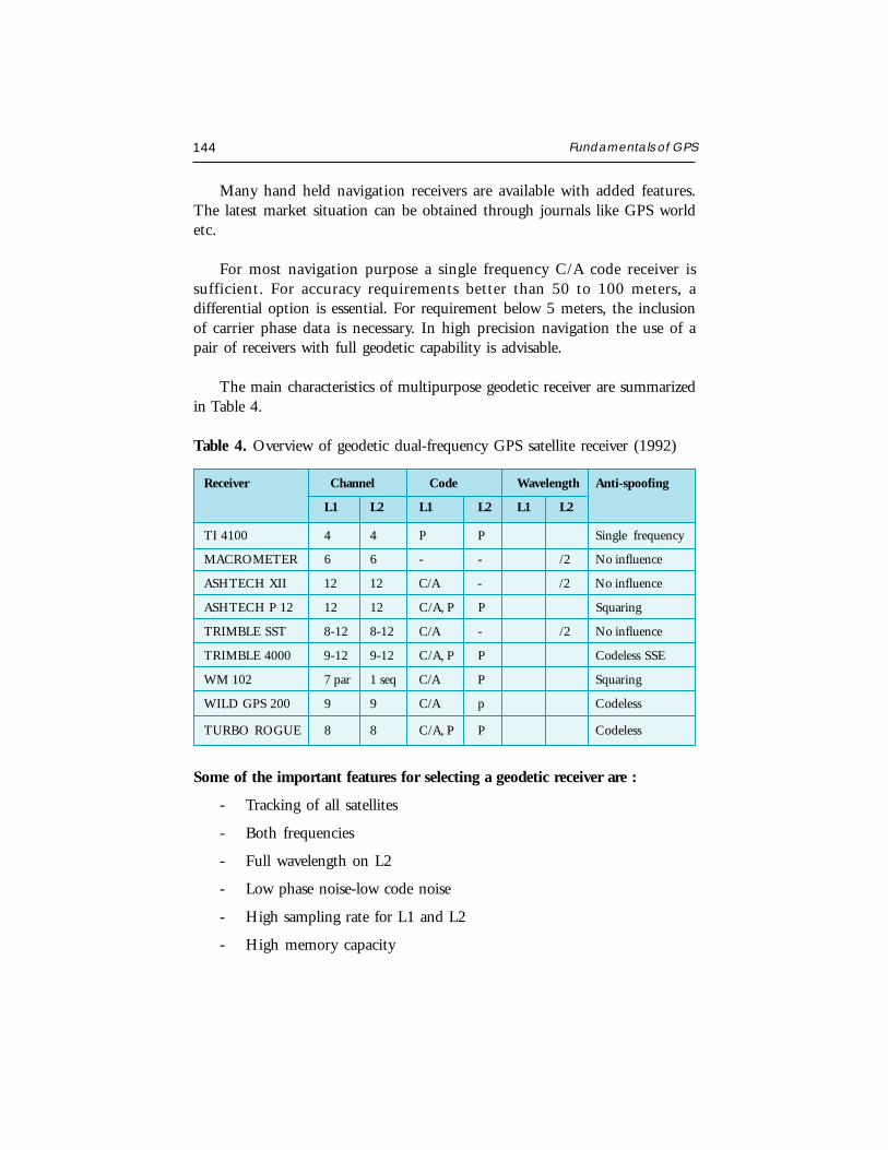
144 Fundamentals of GPS
Many hand held navigation receivers are available with added features.The latest market situation can be obtained through journals like GPS worldetc.
For most navigation purpose a single frequency C/A code receiver issufficient. For accuracy requirements better than 50 to 100 meters, adifferential option is essential. For requirement below 5 meters, the inclusionof carrier phase data is necessary. In high precision navigation the use of apair of receivers with full geodetic capability is advisable.
The main characteristics of multipurpose geodetic receiver are summarizedin Table 4.
Table 4. Overview of geodetic dual-frequency GPS satellite receiver (1992)
Receiver Channel Code Wavelength Anti-spoofing
L1 L2 L1 L2 L1 L2
TI 4100 4 4 P P Single frequency
MACROMETER 6 6 - - /2 No influence
ASHTECH XII 12 12 C/A - /2 No influence
ASHTECH P 12 12 12 C/A, P P Squaring
TRIMBLE SST 8-12 8-12 C/A - /2 No influence
TRIMBLE 4000 9-12 9-12 C/A, P P Codeless SSE
WM 102 7 par 1 seq C/A P Squaring
WILD GPS 200 9 9 C/A p Codeless
TURBO ROGUE 8 8 C/A, P P Codeless
Some of the important features for selecting a geodetic receiver are :
- Tracking of all satellites
- Both frequencies
- Full wavelength on L2
- Low phase noise-low code noise
- High sampling rate for L1 and L2
- High memory capacity
P.L.N. Raju 145
- Low power consumption
- Full operational capability under anti spoofing condition
Further, it is recommended to use dual frequency receiver to minimizeion-spherical influences and take advantages in ambiguity solution.
Accuracy
In general, an SPS receiver can provide position information with an errorof less than 25 meter and velocity information with an error less than 5 metersper second. Upto 2 May 2000 U.S Government has activated SelectiveAvailability (SA) to maintain optimum military effectiveness. SelectiveAvailability inserts random errors into the ephemeris information broadcastby the satellites, which reduces the SPS accuracy to around 100 meters.
For many applications, 100-meter accuracy is more than acceptable. Forapplications that require much greater accuracy, the effects of SA andenvironmentally produced errors can be overcome by using a technique calledDifferential GPS (DGPS), which increases overall accuracy.
Differential Theory
Differential positioning is technique that allows overcoming the effects ofenvironmental errors and SA on the GPS signals to produce a highly accurateposition fix. This is done by determining the amount of the positioning errorand applying it to position fixes that were computed from collected data.
Typically, the horizontal accuracy of a single position fix from a GPSreceiver is 15 meter RMS (root-mean square) or better. If the distribution offixes about the true position is circular normal with zero mean, an accuracyof 15 meters RMS implies that about 63% of the fixes obtained during asession are within 15 meters of the true position.
Types of Errors
There are two types of positioning errors: correctable and non-correctable.Correctable errors are the errors that are essentially the same for two GPSreceivers in the same area. Non-correctable errors cannot be correlated betweentwo GPS receivers in the same area.
146 Fundamentals of GPS
Correctable Errors
Sources of correctable errors include satellite clock, ephemeris data andionosphere and tropospheric delay. If implemented, SA may also cause acorrectable positioning error. Clock errors and ephemeris errors originate withthe GPS satellite. A clock error is a slowly changing error that appears as abias on the pseudorange measurement made by a receiver. An ephemeris erroris a residual error in the data used by a receiver to locate a satellite in space.
Ionosphere delay errors and tropospheric delay errors are caused byatmospheric conditions. Ionospheric delay is caused by the density of electronsin the ionosphere along the signal path. A tropspheric delay is related tohumidity, temperature, and altitude along the signal path. Usually, atropospheric error is smaller than an ionospheric error.
Another correctable error is caused by SA which is used by U.SDepartment of Defence to introduce errors into Standard Positioning Service(SPS) GPS signals to degrade fix accuracy.
The amount of error and direction of the error at any given time doesnot change rapidly. Therefore, two GPS receivers that are sufficiently closetogether will observe the same fix error, and the size of the fix error can bedetermined.
Non-Correctable Errors
Non-correctable errors cannot be correlated between two GPS receiversthat are located in the same general area. Sources of non-correctable errorsinclude receiver noise, which is unavoidably inherent in any receiver, andmultipath errors, which are environmental. Multi-path errors are caused bythe receiver “seeing” reflections of signals that have bounced off of surroundingobjects. The sub-meter antenna is multipath-resistant; its use is required whenlogging carrier phase data. Neither error can be eliminated with differential,but they can be reduced substantially with position fix averaging. The errorsources and the approximate RMS error range are given in the Table 5.
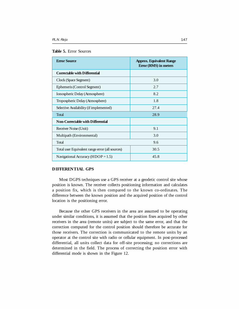
P.L.N. Raju 147
Table 5. Error Sources
Error Source Approx. Equivalent RangeError (RMS) in meters
Correctable with Differential
Clock (Space Segment) 3.0
Ephemeris (Control Segment) 2.7
Ionospheric Delay (Atmosphere) 8.2
Tropospheric Delay (Atmosphere) 1.8
Selective Availability (if implemented) 27.4
Total 28.9
Non-Correctable with Differential
Receiver Noise (Unit) 9.1
Multipath (Environmental) 3.0
Total 9.6
Total user Equivalent range error (all sources) 30.5
Navigational Accuracy (HDOP = 1.5) 45.8
DIFFERENTIAL GPS
Most DGPS techniques use a GPS receiver at a geodetic control site whoseposition is known. The receiver collects positioning information and calculatesa position fix, which is then compared to the known co-ordinates. Thedifference between the known position and the acquired position of the controllocation is the positioning error.
Because the other GPS receivers in the area are assumed to be operatingunder similar conditions, it is assumed that the position fixes acquired by otherreceivers in the area (remote units) are subject to the same error, and that thecorrection computed for the control position should therefore be accurate forthose receivers. The correction is communicated to the remote units by anoperator at the control site with radio or cellular equipment. In post-processeddifferential, all units collect data for off-site processing; no corrections aredetermined in the field. The process of correcting the position error withdifferential mode is shown in the Figure 12.
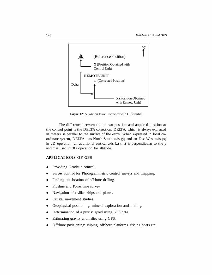
148 Fundamentals of GPS
The difference between the known position and acquired position atthe control point is the DELTA correction. DELTA, which is always expressedin meters, is parallel to the surface of the earth. When expressed in local co-ordinate system, DELTA uses North-South axis (y) and an East-West axis (x)in 2D operation; an additional vertical axis (z) that is perpendicular to the yand x is used in 3D operation for altitude.
APPLICATIONS OF GPS
Providing Geodetic control.
Survey control for Photogrammetric control surveys and mapping.
Finding out location of offshore drilling.
Pipeline and Power line survey.
Navigation of civilian ships and planes.
Crustal movement studies.
Geophysical positioning, mineral exploration and mining.
Determination of a precise geoid using GPS data.
Estimating gravity anomalies using GPS.
Offshore positioning: shiping, offshore platforms, fishing boats etc.
Figure 12: A Position Error Corrected with Differential
(Reference Position)
X (Position Obtained withControl Unit)
REMOTE UNITi (Corrected Position)
X (Position Obtainedwith Remote Unit)
Delta
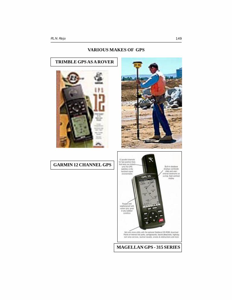
P.L.N. Raju 149
TRIMBLE GPS AS A ROVER
GARMIN 12 CHANNEL GPS
MAGELLAN GPS - 315 SERIES
VARIOUS MAKES OF GPS

150 Fundamentals of GPS
CONCLUSIONS
Global Positioning System (GPS) is currently designed to providenavigational accuracy of ±10 m to ±15 m. However, sub meter accuracy indifferential mode has been achieved and it has been proved that broad varietiesof problems in geodesy and geo-dynamics can be tackled through GPS. GPSservice consists of three components, viz. space, control and user.
REFERENCES
GPS Positioning Guide: A user guide to the Global Positioning System. Natural Resources,Canada. URC : uttp://www.geod.nrcan.gc.ca
GPS World Periodicals.
Proceedings of ION, GPS, 2002. Portland, Oregon, USA Sept. 2002.
Seeber, Gunter 2003. Satellite Geodesy (2nd Edition). Walter de Gruyter Inc. ISBN : 3110175495.
SPATIAL DATA ANALYSIS
P.L.N. RajuGeoinformatics DivisionIndian Institute of Remote Sensing, Dehra Dun
Abstract : Spatial analysis is the vital part of GIS. Spatial analysis in GIS involvesthree types of operations- attribute query (also known as non-spatial), spatial queryand generation of new data sets from the original databases. Various spatial analysismethods viz. single/multiplayer operations/overlay; spatial modeling; geometricmodeling; point pattern analysis; network analysis; surface analysis; raster/grid
analysis etc. are discussed in detail in this paper.
INTRODUCTION
Geographic analysis allows us to study and understand the real worldprocesses by developing and applying manipulation, analysis criteria andmodels and to carryout integrated modeling. These criteria illuminateunderlying trends in geographic data, making new information available. AGIS enhances this process by providing tools, which can be combined inmeaningful sequence to reveal new or previously unidentified relationshipswithin or between data sets, thus increasing better understanding of real world.The results of geographic analysis can be commercial in the form of maps,reports or both. Integration involves bringing together diverse information froma variety of sources and analysis of multi-parameter data to provide answersand solutions to defined problems.
Spatial analysis is the vital part of GIS. It can be done in two ways. Oneis the vector-based and the other is raster-based analysis. Since the advent ofGIS in the 1980s, many government agencies have invested heavily in GISinstallations, including the purchase of hardware and software and theconstruction of mammoth databases. Two fundamental functions of GIS havebeen widely realized: generation of maps and generation of tabular reports.
Satellite Remote Sensing and GIS Applications in Agricultural Meteorologypp. 151-174
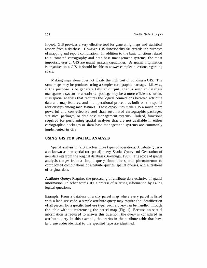
152 Spatial Data Analysis
Indeed, GIS provides a very effective tool for generating maps and statisticalreports from a database. However, GIS functionality far exceeds the purposesof mapping and report compilation. In addition to the basic functions relatedto automated cartography and data base management systems, the mostimportant uses of GIS are spatial analysis capabilities. As spatial informationis organized in a GIS, it should be able to answer complex questions regardingspace.
Making maps alone does not justify the high cost of building a GIS. Thesame maps may be produced using a simpler cartographic package. Likewise,if the purpose is to generate tabular output, then a simpler databasemanagement system or a statistical package may be a more efficient solution.It is spatial analysis that requires the logical connections between attributedata and map features, and the operational procedures built on the spatialrelationships among map features. These capabilities make GIS a much morepowerful and cost-effective tool than automated cartographic packages,statistical packages, or data base management systems. Indeed, functionsrequired for performing spatial analyses that are not available in eithercartographic packages or data base management systems are commonlyimplemented in GIS.
USING GIS FOR SPATIAL ANALYSIS
Spatial analysis in GIS involves three types of operations: Attribute Query-also known as non-spatial (or spatial) query, Spatial Query and Generation ofnew data sets from the original database (Bwozough, 1987). The scope of spatialanalysis ranges from a simple query about the spatial phenomenon tocomplicated combinations of attribute queries, spatial queries, and alterationsof original data.
Attribute Query: Requires the processing of attribute data exclusive of spatialinformation. In other words, it’s a process of selecting information by askinglogical questions.
Example: From a database of a city parcel map where every parcel is listedwith a land use code, a simple attribute query may require the identificationof all parcels for a specific land use type. Such a query can be handled throughthe table without referencing the parcel map (Fig. 1). Because no spatialinformation is required to answer this question, the query is considered anattribute query. In this example, the entries in the attribute table that haveland use codes identical to the specified type are identified.
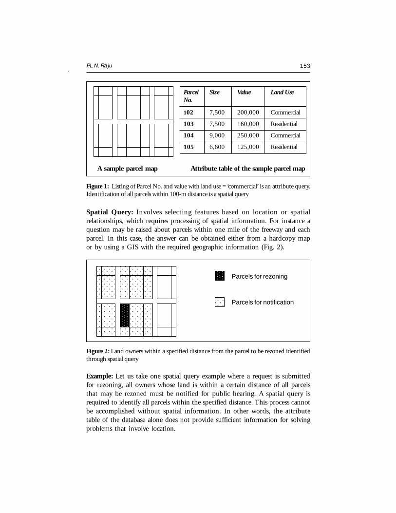
P.L.N. Raju 153
Spatial Query: Involves selecting features based on location or spatialrelationships, which requires processing of spatial information. For instance aquestion may be raised about parcels within one mile of the freeway and eachparcel. In this case, the answer can be obtained either from a hardcopy mapor by using a GIS with the required geographic information (Fig. 2).
Parcel Size Value Land UseNo.
102 7,500 200,000 Commercial
103 7,500 160,000 Residential
104 9,000 250,000 Commercial
105 6,600 125,000 Residential
A sample parcel map Attribute table of the sample parcel map
Figure 1: Listing of Parcel No. and value with land use = ‘commercial’ is an attribute query.Identification of all parcels within 100-m distance is a spatial query
Parcels for rezoning
Parcels for notification
Figure 2: Land owners within a specified distance from the parcel to be rezoned identifiedthrough spatial query
Example: Let us take one spatial query example where a request is submittedfor rezoning, all owners whose land is within a certain distance of all parcelsthat may be rezoned must be notified for public hearing. A spatial query isrequired to identify all parcels within the specified distance. This process cannotbe accomplished without spatial information. In other words, the attributetable of the database alone does not provide sufficient information for solvingproblems that involve location.
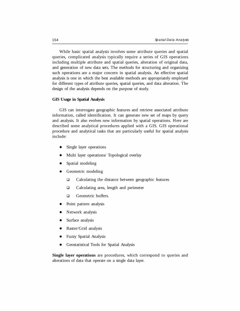
154 Spatial Data Analysis
While basic spatial analysis involves some attribute queries and spatialqueries, complicated analysis typically require a series of GIS operationsincluding multiple attribute and spatial queries, alteration of original data,and generation of new data sets. The methods for structuring and organizingsuch operations are a major concern in spatial analysis. An effective spatialanalysis is one in which the best available methods are appropriately employedfor different types of attribute queries, spatial queries, and data alteration. Thedesign of the analysis depends on the purpose of study.
GIS Usage in Spatial Analysis
GIS can interrogate geographic features and retrieve associated attributeinformation, called identification. It can generate new set of maps by queryand analysis. It also evolves new information by spatial operations. Here aredescribed some analytical procedures applied with a GIS. GIS operationalprocedure and analytical tasks that are particularly useful for spatial analysisinclude:
Single layer operations
Multi layer operations/ Topological overlay
Spatial modeling
Geometric modeling
Calculating the distance between geographic features
Calculating area, length and perimeter
Geometric buffers.
Point pattern analysis
Network analysis
Surface analysis
Raster/Grid analysis
Fuzzy Spatial Analysis
Geostatistical Tools for Spatial Analysis
Single layer operations are procedures, which correspond to queries andalterations of data that operate on a single data layer.
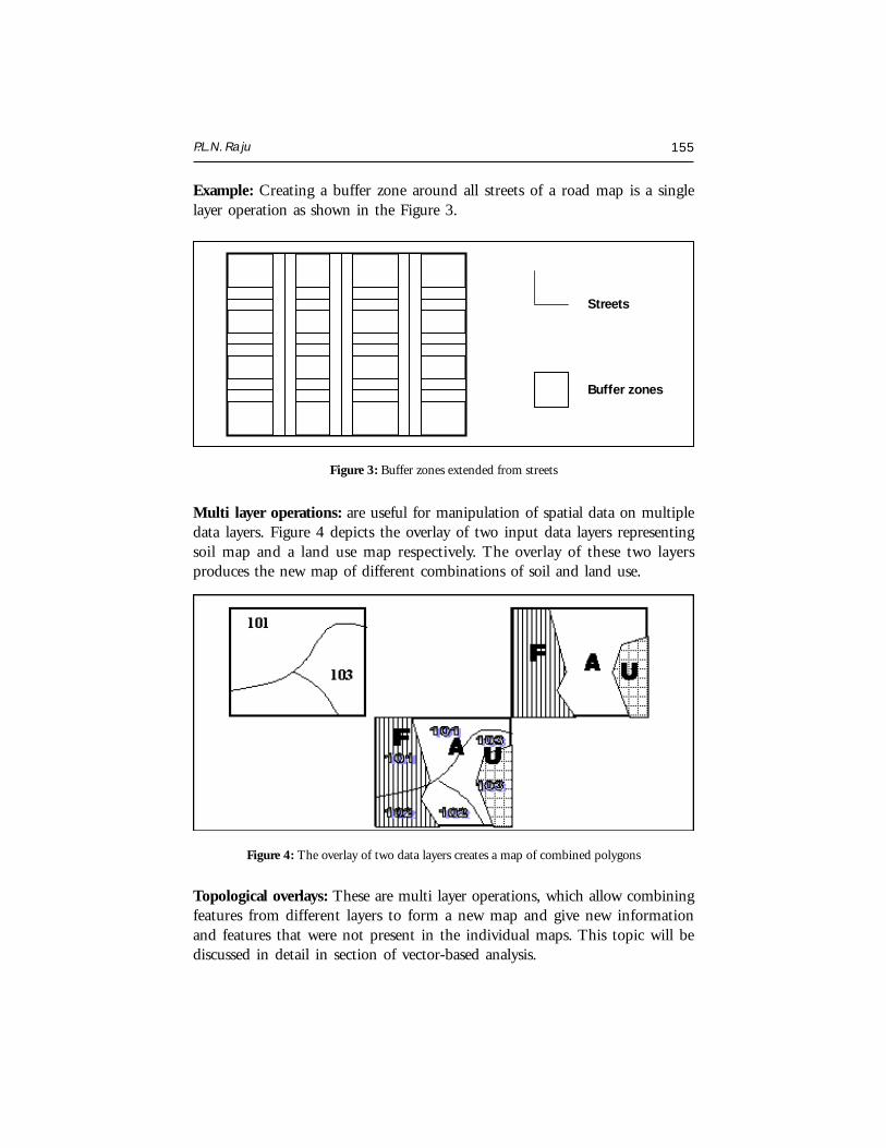
P.L.N. Raju 155
Example: Creating a buffer zone around all streets of a road map is a singlelayer operation as shown in the Figure 3.
Figure 3: Buffer zones extended from streets
Streets
Buffer zones
Multi layer operations: are useful for manipulation of spatial data on multipledata layers. Figure 4 depicts the overlay of two input data layers representingsoil map and a land use map respectively. The overlay of these two layersproduces the new map of different combinations of soil and land use.
Figure 4: The overlay of two data layers creates a map of combined polygons
Topological overlays: These are multi layer operations, which allow combiningfeatures from different layers to form a new map and give new informationand features that were not present in the individual maps. This topic will bediscussed in detail in section of vector-based analysis.
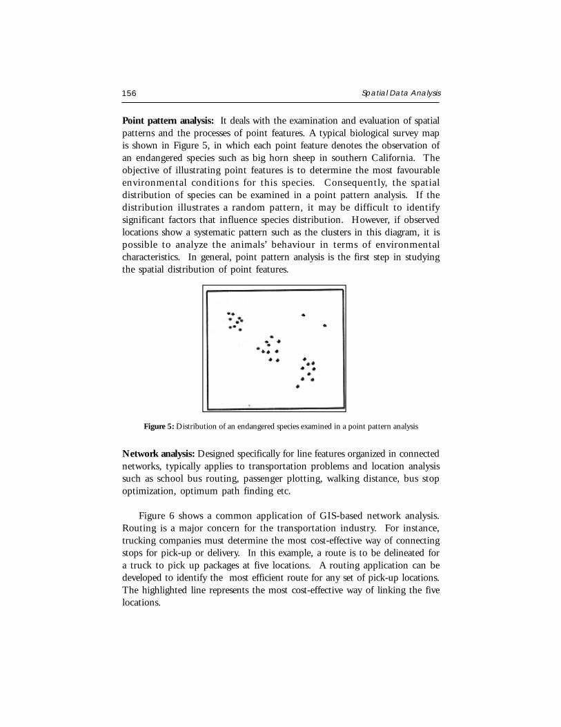
156 Spatial Data Analysis
Point pattern analysis: It deals with the examination and evaluation of spatialpatterns and the processes of point features. A typical biological survey mapis shown in Figure 5, in which each point feature denotes the observation ofan endangered species such as big horn sheep in southern California. Theobjective of illustrating point features is to determine the most favourableenvironmental conditions for this species. Consequently, the spatialdistribution of species can be examined in a point pattern analysis. If thedistribution illustrates a random pattern, it may be difficult to identifysignificant factors that influence species distribution. However, if observedlocations show a systematic pattern such as the clusters in this diagram, it ispossible to analyze the animals’ behaviour in terms of environmentalcharacteristics. In general, point pattern analysis is the first step in studyingthe spatial distribution of point features.
Figure 5: Distribution of an endangered species examined in a point pattern analysis
Network analysis: Designed specifically for line features organized in connectednetworks, typically applies to transportation problems and location analysissuch as school bus routing, passenger plotting, walking distance, bus stopoptimization, optimum path finding etc.
Figure 6 shows a common application of GIS-based network analysis.Routing is a major concern for the transportation industry. For instance,trucking companies must determine the most cost-effective way of connectingstops for pick-up or delivery. In this example, a route is to be delineated fora truck to pick up packages at five locations. A routing application can bedeveloped to identify the most efficient route for any set of pick-up locations.The highlighted line represents the most cost-effective way of linking the fivelocations.
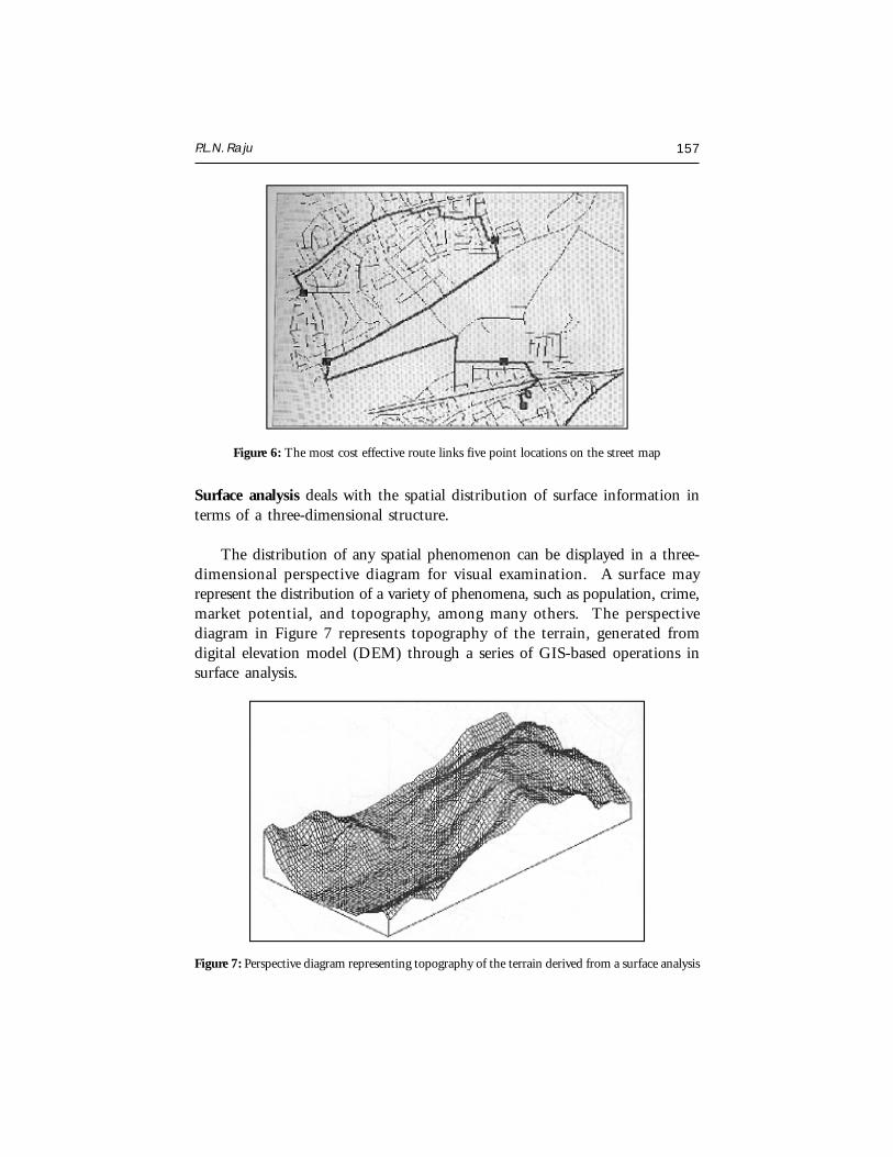
P.L.N. Raju 157
Figure 6: The most cost effective route links five point locations on the street map
Surface analysis deals with the spatial distribution of surface information interms of a three-dimensional structure.
The distribution of any spatial phenomenon can be displayed in a three-dimensional perspective diagram for visual examination. A surface mayrepresent the distribution of a variety of phenomena, such as population, crime,market potential, and topography, among many others. The perspectivediagram in Figure 7 represents topography of the terrain, generated fromdigital elevation model (DEM) through a series of GIS-based operations insurface analysis.
Figure 7: Perspective diagram representing topography of the terrain derived from a surface analysis
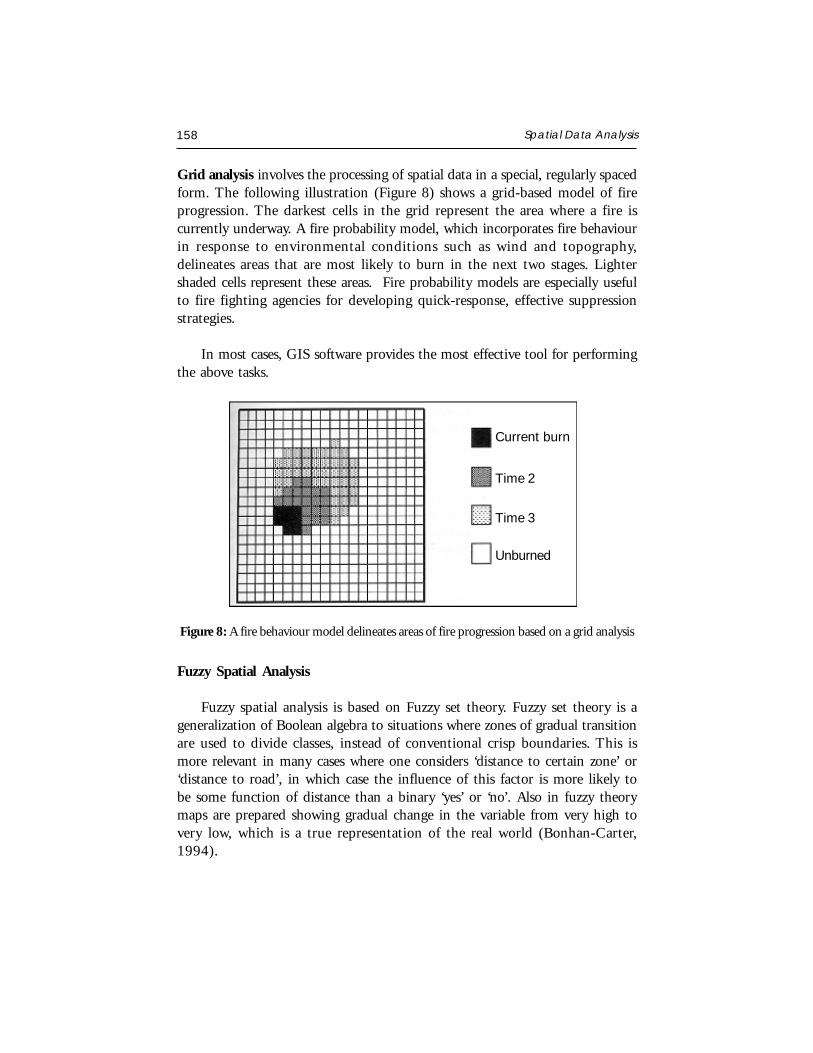
158 Spatial Data Analysis
Grid analysis involves the processing of spatial data in a special, regularly spacedform. The following illustration (Figure 8) shows a grid-based model of fireprogression. The darkest cells in the grid represent the area where a fire iscurrently underway. A fire probability model, which incorporates fire behaviourin response to environmental conditions such as wind and topography,delineates areas that are most likely to burn in the next two stages. Lightershaded cells represent these areas. Fire probability models are especially usefulto fire fighting agencies for developing quick-response, effective suppressionstrategies.
In most cases, GIS software provides the most effective tool for performingthe above tasks.
Figure 8: A fire behaviour model delineates areas of fire progression based on a grid analysis
Fuzzy Spatial Analysis
Fuzzy spatial analysis is based on Fuzzy set theory. Fuzzy set theory is ageneralization of Boolean algebra to situations where zones of gradual transitionare used to divide classes, instead of conventional crisp boundaries. This ismore relevant in many cases where one considers ‘distance to certain zone’ or‘distance to road’, in which case the influence of this factor is more likely tobe some function of distance than a binary ‘yes’ or ‘no’. Also in fuzzy theorymaps are prepared showing gradual change in the variable from very high tovery low, which is a true representation of the real world (Bonhan-Carter,1994).
Current burn
Time 2
Time 3
Unburned
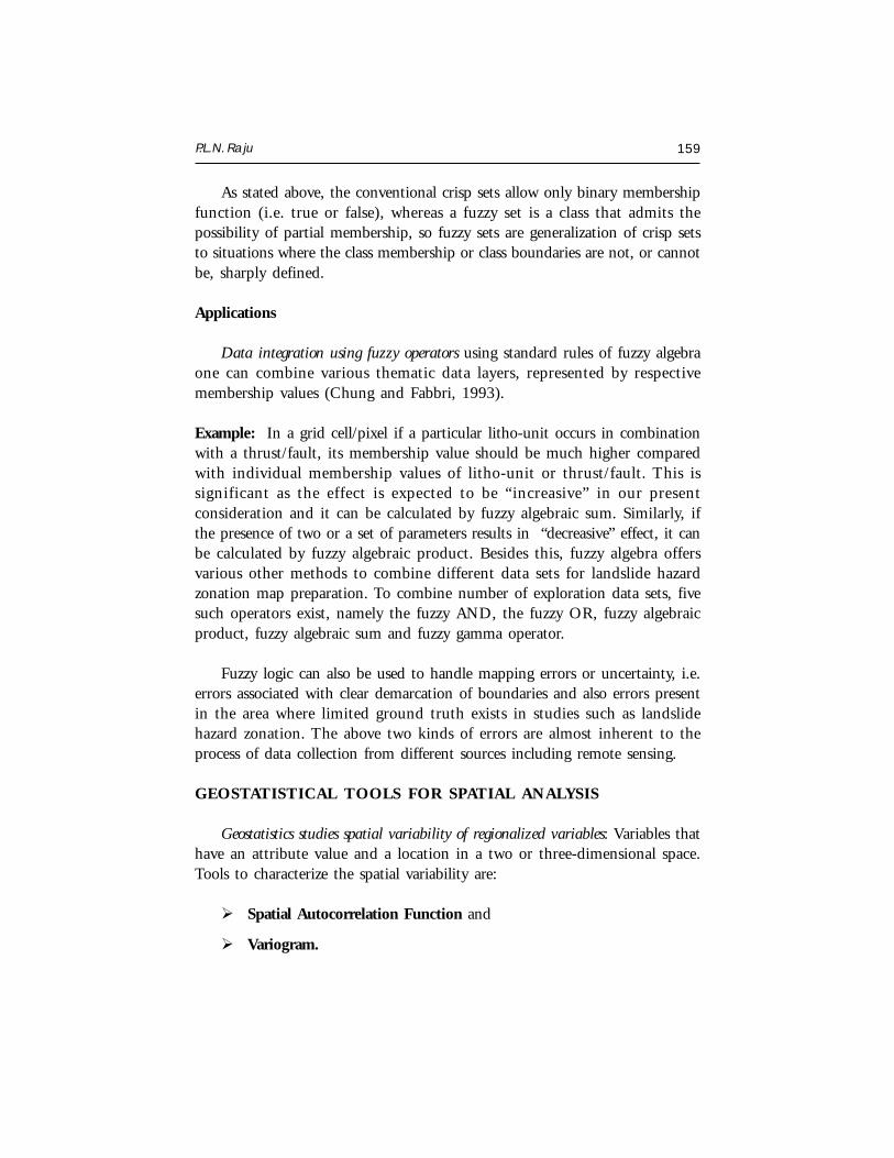
P.L.N. Raju 159
As stated above, the conventional crisp sets allow only binary membershipfunction (i.e. true or false), whereas a fuzzy set is a class that admits thepossibility of partial membership, so fuzzy sets are generalization of crisp setsto situations where the class membership or class boundaries are not, or cannotbe, sharply defined.
Applications
Data integration using fuzzy operators using standard rules of fuzzy algebraone can combine various thematic data layers, represented by respectivemembership values (Chung and Fabbri, 1993).
Example: In a grid cell/pixel if a particular litho-unit occurs in combinationwith a thrust/fault, its membership value should be much higher comparedwith individual membership values of litho-unit or thrust/fault. This issignificant as the effect is expected to be “increasive” in our presentconsideration and it can be calculated by fuzzy algebraic sum. Similarly, ifthe presence of two or a set of parameters results in “decreasive” effect, it canbe calculated by fuzzy algebraic product. Besides this, fuzzy algebra offersvarious other methods to combine different data sets for landslide hazardzonation map preparation. To combine number of exploration data sets, fivesuch operators exist, namely the fuzzy AND, the fuzzy OR, fuzzy algebraicproduct, fuzzy algebraic sum and fuzzy gamma operator.
Fuzzy logic can also be used to handle mapping errors or uncertainty, i.e.errors associated with clear demarcation of boundaries and also errors presentin the area where limited ground truth exists in studies such as landslidehazard zonation. The above two kinds of errors are almost inherent to theprocess of data collection from different sources including remote sensing.
GEOSTATISTICAL TOOLS FOR SPATIAL ANALYSIS
Geostatistics studies spatial variability of regionalized variables: Variables thathave an attribute value and a location in a two or three-dimensional space.Tools to characterize the spatial variability are:
Spatial Autocorrelation Function and
Variogram.
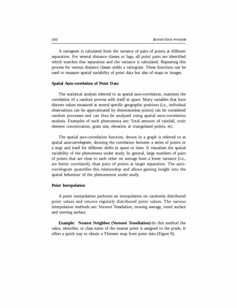
160 Spatial Data Analysis
A variogram is calculated from the variance of pairs of points at differentseparation. For several distance classes or lags, all point pairs are identifiedwhich matches that separation and the variance is calculated. Repeating thisprocess for various distance classes yields a variogram. These functions can beused to measure spatial variability of point data but also of maps or images.
Spatial Auto-correlation of Point Data
The statistical analysis referred to as spatial auto-correlation, examines thecorrelation of a random process with itself in space. Many variables that havediscrete values measured at several specific geographic positions (i.e., individualobservations can be approximated by dimensionless points) can be consideredrandom processes and can thus be analyzed using spatial auto-correlationanalysis. Examples of such phenomena are: Total amount of rainfall, toxicelement concentration, grain size, elevation at triangulated points, etc.
The spatial auto-correlation function, shown in a graph is referred to asspatial auto-correlogram, showing the correlation between a series of points ora map and itself for different shifts in space or time. It visualizes the spatialvariability of the phenomena under study. In general, large numbers of pairsof points that are close to each other on average have a lower variance (i.e.,are better correlated), than pairs of points at larger separation. The auto-correlogram quantifies this relationship and allows gaining insight into thespatial behaviour of the phenomenon under study.
Point Interpolation
A point interpolation performs an interpolation on randomly distributedpoint values and returns regularly distributed point values. The variousinterpolation methods are: Voronoi Tesselation, moving average, trend surfaceand moving surface.
Example: Nearest Neighbor (Voronoi Tessellation)-In this method thevalue, identifier, or class name of the nearest point is assigned to the pixels. Itoffers a quick way to obtain a Thiessen map from point data (Figure 9).
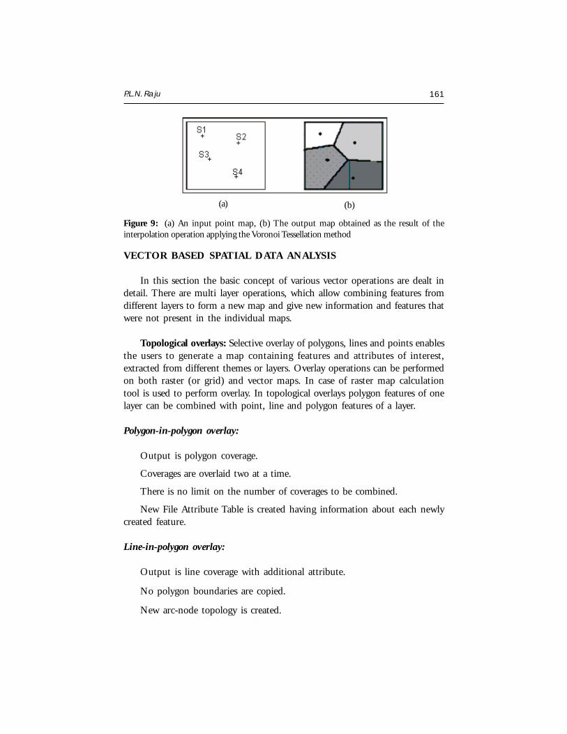
P.L.N. Raju 161
VECTOR BASED SPATIAL DATA ANALYSIS
In this section the basic concept of various vector operations are dealt indetail. There are multi layer operations, which allow combining features fromdifferent layers to form a new map and give new information and features thatwere not present in the individual maps.
Topological overlays: Selective overlay of polygons, lines and points enablesthe users to generate a map containing features and attributes of interest,extracted from different themes or layers. Overlay operations can be performedon both raster (or grid) and vector maps. In case of raster map calculationtool is used to perform overlay. In topological overlays polygon features of onelayer can be combined with point, line and polygon features of a layer.
Polygon-in-polygon overlay:
Output is polygon coverage.
Coverages are overlaid two at a time.
There is no limit on the number of coverages to be combined.
New File Attribute Table is created having information about each newlycreated feature.
Line-in-polygon overlay:
Output is line coverage with additional attribute.
No polygon boundaries are copied.
New arc-node topology is created.
Figure 9: (a) An input point map, (b) The output map obtained as the result of theinterpolation operation applying the Voronoi Tessellation method
(a) (b)
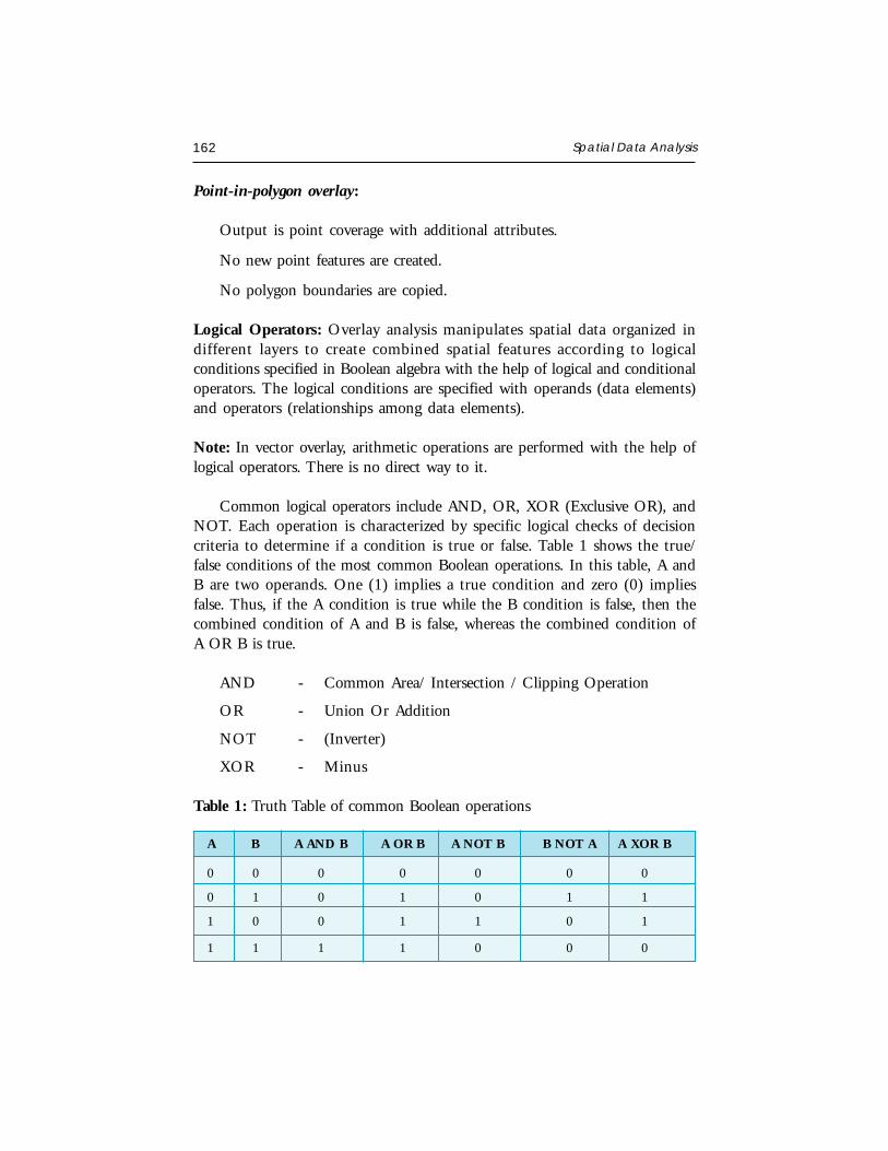
162 Spatial Data Analysis
Point-in-polygon overlay:
Output is point coverage with additional attributes.
No new point features are created.
No polygon boundaries are copied.
Logical Operators: Overlay analysis manipulates spatial data organized indifferent layers to create combined spatial features according to logicalconditions specified in Boolean algebra with the help of logical and conditionaloperators. The logical conditions are specified with operands (data elements)and operators (relationships among data elements).
Note: In vector overlay, arithmetic operations are performed with the help oflogical operators. There is no direct way to it.
Common logical operators include AND, OR, XOR (Exclusive OR), andNOT. Each operation is characterized by specific logical checks of decisioncriteria to determine if a condition is true or false. Table 1 shows the true/false conditions of the most common Boolean operations. In this table, A andB are two operands. One (1) implies a true condition and zero (0) impliesfalse. Thus, if the A condition is true while the B condition is false, then thecombined condition of A and B is false, whereas the combined condition ofA OR B is true.
AND - Common Area/ Intersection / Clipping Operation
OR - Union Or Addition
NOT - (Inverter)
XOR - Minus
Table 1: Truth Table of common Boolean operations
A B A AND B A OR B A NOT B B NOT A A XOR B
0 0 0 0 0 0 0
0 1 0 1 0 1 1
1 0 0 1 1 0 1
1 1 1 1 0 0 0
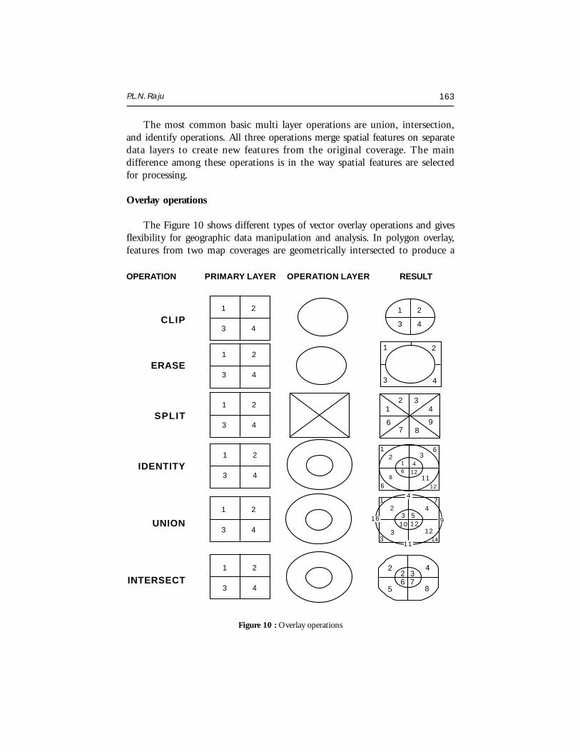
P.L.N. Raju 163
The most common basic multi layer operations are union, intersection,and identify operations. All three operations merge spatial features on separatedata layers to create new features from the original coverage. The maindifference among these operations is in the way spatial features are selectedfor processing.
Overlay operations
The Figure 10 shows different types of vector overlay operations and givesflexibility for geographic data manipulation and analysis. In polygon overlay,features from two map coverages are geometrically intersected to produce a
Figure 10 : Overlay operations
OPERATION PRIMARY LAYER OPERATION LAYER RESULT
CLIP
ERASE
SPLIT
IDENTITY
UNION
INTERSECT
1 2
3 4
1 2
3 4
1 2
3 4
1 2
3 4
1 2
3 4
1 2
3 4
1 2
3 4
1 2
3 4
12 3
4
67 8
9
2 4
5 8
2 36 7
1 72 4
3 12
3 510 12
3 14
16 9
11
4
2 3
8 116 12
1 46 12
1 6
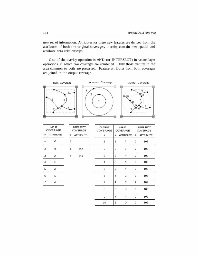
164 Spatial Data Analysis
new set of information. Attributes for these new features are derived from theattributes of both the original coverages, thereby contain new spatial andattribute data relationships.
One of the overlay operation is AND (or INTERSECT) in vector layeroperations, in which two coverages are combined. Only those features in thearea common to both are preserved. Feature attributes from both coveragesare joined in the output coverage.
Input Coverage Intersect Coverage Output Coverage
INPUTCOVERAGE
# ATTRIBUTE
1 A
2 B
3 A
4 C
5 A
6 D
7 A
INTERSECTCOVERAGE
# ATTRIBUTE
1
2 102
3 103
OUTPUT INPUT INTERSECTCOVERAGE COVERAGE COVERAGE
# # ATTRIBUTE # ATTRIBUTE
1 1 A 2 102
2 2 B 2 102
3 3 A 2 102
4 3 A 3 103
5 5 A 3 103
6 4 C 3 103
7 4 C 2 102
8 6 D 3 103
9 7 A 2 102
10 6 D 2 102
P.L.N. Raju 165
RASTER BASED SPATIAL DATA ANALYSIS
Present section discusses operational procedures and quantitative methodsfor the analysis of spatial data in raster format. In raster analysis, geographicunits are regularly spaced, and the location of each unit is referenced by rowand column positions. Because geographic units are of equal size and identicalshape, area adjustment of geographic units is unnecessary and spatialproperties of geographic entities are relatively easy to trace. All cells in a gridhave a positive position reference, following the left-to-right and top-to-bottomdata scan. Every cell in a grid is an individual unit and must be assigned avalue. Depending on the nature of the grid, the value assigned to a cell canbe an integer or a floating point. When data values are not available forparticular cells, they are described as NODATA cells. NODATA cells differfrom cells containing zero in the sense that zero value is considered to be data.
The regularity in the arrangement of geographic units allows for theunderlying spatial relationships to be efficiently formulated. For instance, thedistance between orthogonal neighbors (neighbors on the same row or column)is always a constant whereas the distance between two diagonal units can alsobe computed as a function of that constant. Therefore, the distance betweenany pair of units can be computed from differences in row and columnpositions. Furthermore, directional information is readily available for anypair of origin and destination cells as long as their positions in the grid areknown.
Advantages of using the Raster Format in Spatial Analysis
Efficient processing: Because geographic units are regularly spaced withidentical spatial properties, multiple layer operations can be processed veryefficiently.
Numerous existing sources: Grids are the common format for numeroussources of spatial information including satellite imagery, scanned aerial photos,and digital elevation models, among others. These data sources have beenadopted in many GIS projects and have become the most common sources ofmajor geographic databases.
Different feature types organized in the same layer: For instance, the samegrid may consist of point features, line features, and area features, as long asdifferent features are assigned different values.
166 Spatial Data Analysis
Grid Format Disadvantages
Data redundancy: When data elements are organized in a regularly spacedsystem, there is a data point at the location of every grid cell, regardlessof whether the data element is needed or not. Although, severalcompression techniques are available, the advantages of gridded data arelost whenever the gridded data format is altered through compression. Inmost cases, the compressed data cannot be directly processed for analysis.Instead, the compressed raster data must first be decompressed in orderto take advantage of spatial regularity.
Resolution confusion: Gridded data give an unnatural look and unrealisticpresentation unless the resolution is sufficiently high. Conversely, spatialresolution dictates spatial properties. For instance, some spatial statisticsderived from a distribution may be different, if spatial resolution varies,which is the result of the well-known scale problem.
Cell value assignment difficulties: Different methods of cell valueassignment may result in quite different spatial patterns.
Grid Operations used in Map Algebra
Common operations in grid analysis consist of the following functions,which are used in Map Algebra to manipulate grid files. The Map Algebralanguage is a programming language developed to perform cartographicmodeling. Map Algebra performs following four basic operations:
Local functions: that work on every single cell,
Focal functions: that process the data of each cell based on the informationof a specified neighborhood,
Zonal functions: that provide operations that work on each group of cellsof identical values, and
Global functions: that work on a cell based on the data of the entiregrid.
The principal functionality of these operations is described here.
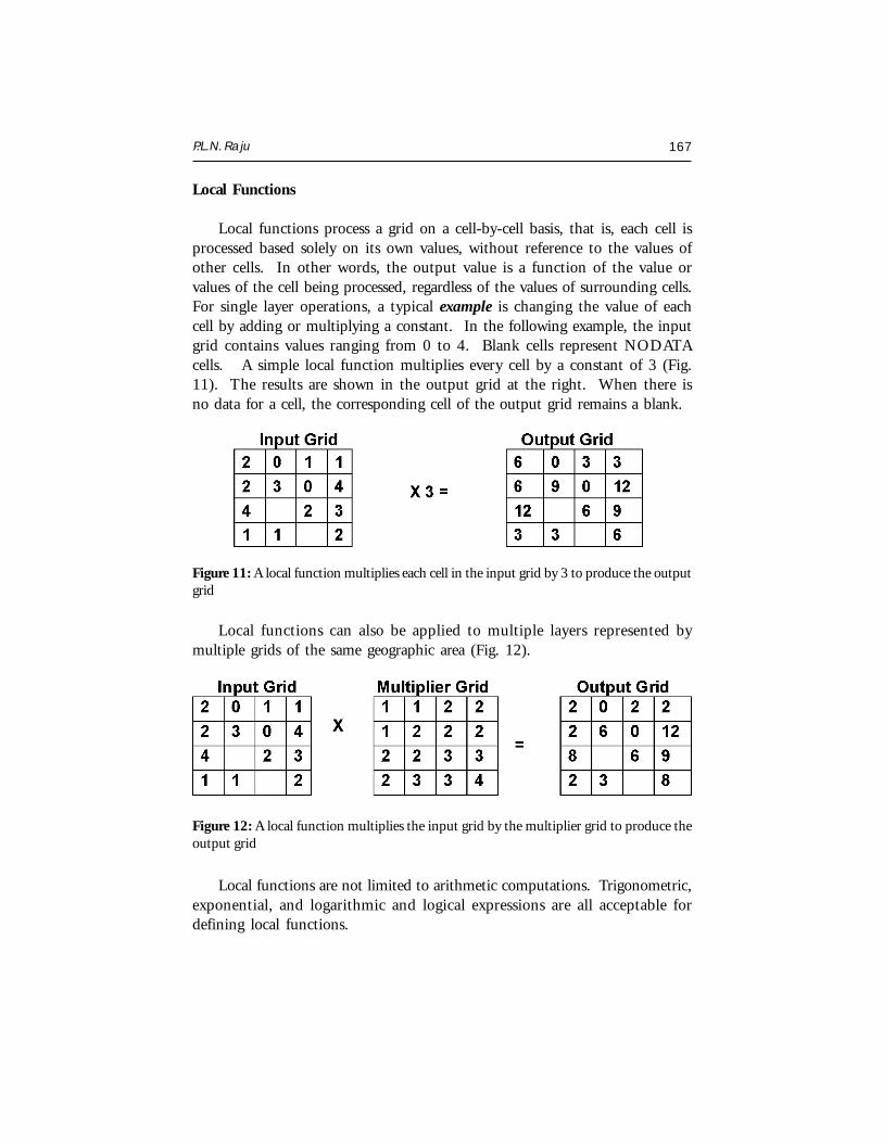
P.L.N. Raju 167
Local Functions
Local functions process a grid on a cell-by-cell basis, that is, each cell isprocessed based solely on its own values, without reference to the values ofother cells. In other words, the output value is a function of the value orvalues of the cell being processed, regardless of the values of surrounding cells.For single layer operations, a typical example is changing the value of eachcell by adding or multiplying a constant. In the following example, the inputgrid contains values ranging from 0 to 4. Blank cells represent NODATAcells. A simple local function multiplies every cell by a constant of 3 (Fig.11). The results are shown in the output grid at the right. When there isno data for a cell, the corresponding cell of the output grid remains a blank.
Figure 11: A local function multiplies each cell in the input grid by 3 to produce the outputgrid
Local functions can also be applied to multiple layers represented bymultiple grids of the same geographic area (Fig. 12).
Figure 12: A local function multiplies the input grid by the multiplier grid to produce theoutput grid
Local functions are not limited to arithmetic computations. Trigonometric,exponential, and logarithmic and logical expressions are all acceptable fordefining local functions.
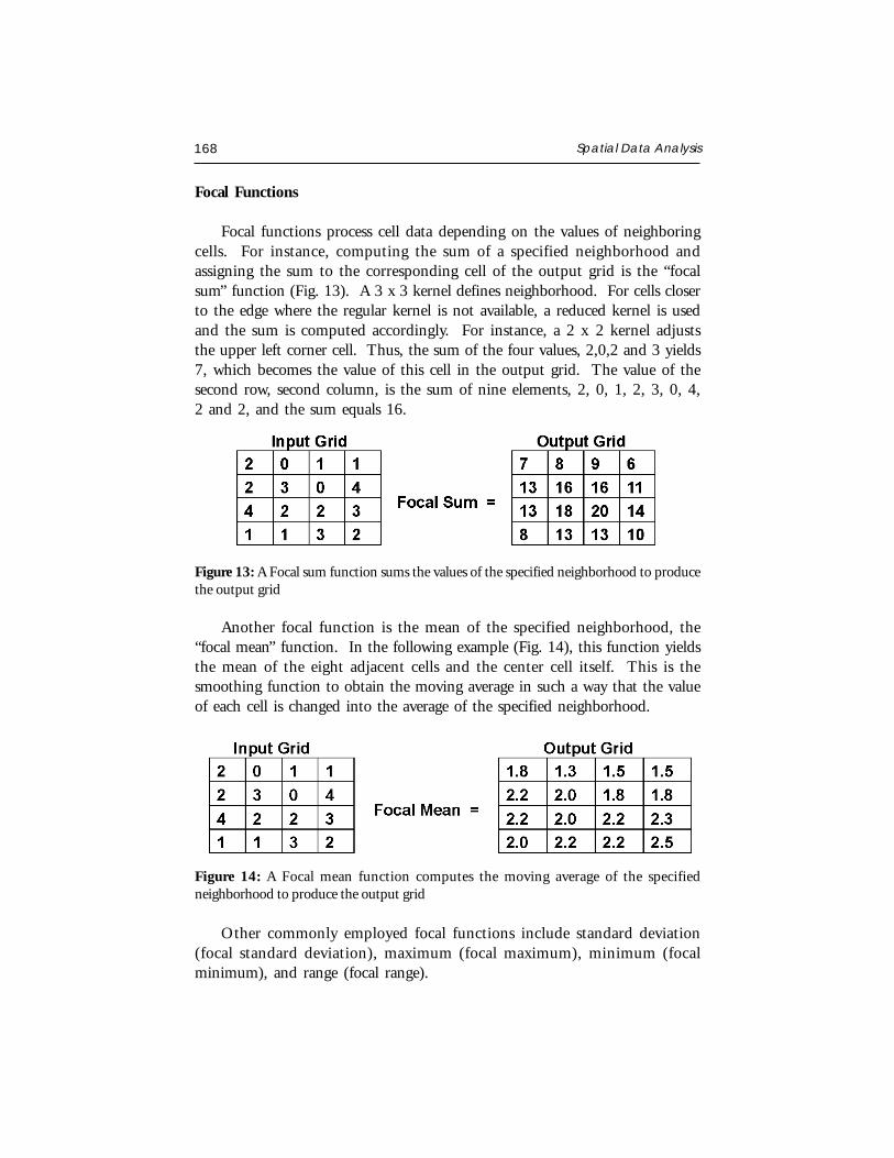
168 Spatial Data Analysis
Focal Functions
Focal functions process cell data depending on the values of neighboringcells. For instance, computing the sum of a specified neighborhood andassigning the sum to the corresponding cell of the output grid is the “focalsum” function (Fig. 13). A 3 x 3 kernel defines neighborhood. For cells closerto the edge where the regular kernel is not available, a reduced kernel is usedand the sum is computed accordingly. For instance, a 2 x 2 kernel adjuststhe upper left corner cell. Thus, the sum of the four values, 2,0,2 and 3 yields7, which becomes the value of this cell in the output grid. The value of thesecond row, second column, is the sum of nine elements, 2, 0, 1, 2, 3, 0, 4,2 and 2, and the sum equals 16.
Figure 13: A Focal sum function sums the values of the specified neighborhood to producethe output grid
Another focal function is the mean of the specified neighborhood, the“focal mean” function. In the following example (Fig. 14), this function yieldsthe mean of the eight adjacent cells and the center cell itself. This is thesmoothing function to obtain the moving average in such a way that the valueof each cell is changed into the average of the specified neighborhood.
Figure 14: A Focal mean function computes the moving average of the specifiedneighborhood to produce the output grid
Other commonly employed focal functions include standard deviation(focal standard deviation), maximum (focal maximum), minimum (focalminimum), and range (focal range).
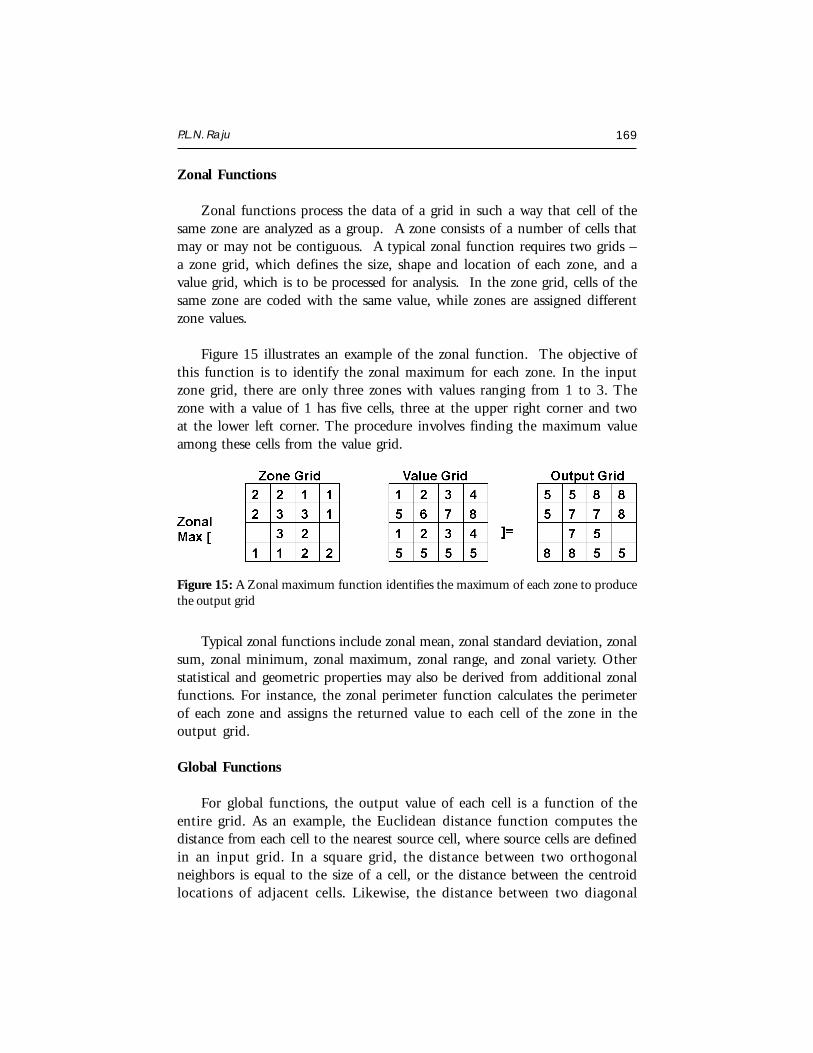
P.L.N. Raju 169
Zonal Functions
Zonal functions process the data of a grid in such a way that cell of thesame zone are analyzed as a group. A zone consists of a number of cells thatmay or may not be contiguous. A typical zonal function requires two grids –a zone grid, which defines the size, shape and location of each zone, and avalue grid, which is to be processed for analysis. In the zone grid, cells of thesame zone are coded with the same value, while zones are assigned differentzone values.
Figure 15 illustrates an example of the zonal function. The objective ofthis function is to identify the zonal maximum for each zone. In the inputzone grid, there are only three zones with values ranging from 1 to 3. Thezone with a value of 1 has five cells, three at the upper right corner and twoat the lower left corner. The procedure involves finding the maximum valueamong these cells from the value grid.
Typical zonal functions include zonal mean, zonal standard deviation, zonalsum, zonal minimum, zonal maximum, zonal range, and zonal variety. Otherstatistical and geometric properties may also be derived from additional zonalfunctions. For instance, the zonal perimeter function calculates the perimeterof each zone and assigns the returned value to each cell of the zone in theoutput grid.
Global Functions
For global functions, the output value of each cell is a function of theentire grid. As an example, the Euclidean distance function computes thedistance from each cell to the nearest source cell, where source cells are definedin an input grid. In a square grid, the distance between two orthogonalneighbors is equal to the size of a cell, or the distance between the centroidlocations of adjacent cells. Likewise, the distance between two diagonal
Figure 15: A Zonal maximum function identifies the maximum of each zone to producethe output grid
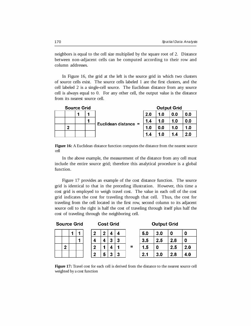
170 Spatial Data Analysis
neighbors is equal to the cell size multiplied by the square root of 2. Distancebetween non-adjacent cells can be computed according to their row andcolumn addresses.
In Figure 16, the grid at the left is the source grid in which two clustersof source cells exist. The source cells labeled 1 are the first clusters, and thecell labeled 2 is a single-cell source. The Euclidean distance from any sourcecell is always equal to 0. For any other cell, the output value is the distancefrom its nearest source cell.
In the above example, the measurement of the distance from any cell mustinclude the entire source grid; therefore this analytical procedure is a globalfunction.
Figure 17 provides an example of the cost distance function. The sourcegrid is identical to that in the preceding illustration. However, this time acost grid is employed to weigh travel cost. The value in each cell of the costgrid indicates the cost for traveling through that cell. Thus, the cost fortraveling from the cell located in the first row, second column to its adjacentsource cell to the right is half the cost of traveling through itself plus half thecost of traveling through the neighboring cell.
Figure 16: A Euclidean distance function computes the distance from the nearest sourcecell
Figure 17: Travel cost for each cell is derived from the distance to the nearest source cellweighted by a cost function
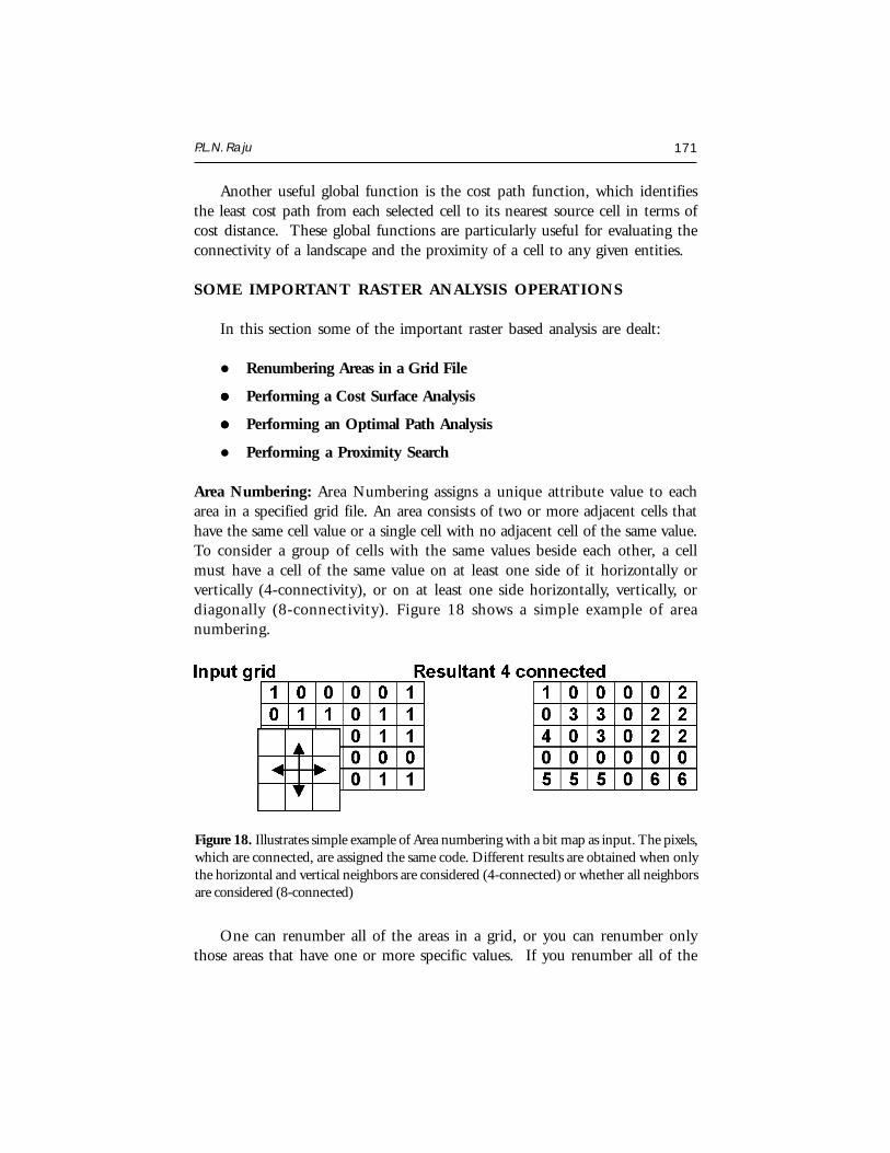
P.L.N. Raju 171
Another useful global function is the cost path function, which identifiesthe least cost path from each selected cell to its nearest source cell in terms ofcost distance. These global functions are particularly useful for evaluating theconnectivity of a landscape and the proximity of a cell to any given entities.
SOME IMPORTANT RASTER ANALYSIS OPERATIONS
In this section some of the important raster based analysis are dealt:
Renumbering Areas in a Grid File
Performing a Cost Surface Analysis
Performing an Optimal Path Analysis
Performing a Proximity Search
Area Numbering: Area Numbering assigns a unique attribute value to eacharea in a specified grid file. An area consists of two or more adjacent cells thathave the same cell value or a single cell with no adjacent cell of the same value.To consider a group of cells with the same values beside each other, a cellmust have a cell of the same value on at least one side of it horizontally orvertically (4-connectivity), or on at least one side horizontally, vertically, ordiagonally (8-connectivity). Figure 18 shows a simple example of areanumbering.
Figure 18. Illustrates simple example of Area numbering with a bit map as input. The pixels,which are connected, are assigned the same code. Different results are obtained when onlythe horizontal and vertical neighbors are considered (4-connected) or whether all neighborsare considered (8-connected)
One can renumber all of the areas in a grid, or you can renumber onlythose areas that have one or more specific values. If you renumber all of the
172 Spatial Data Analysis
areas, Area Number assigns a value of 1 to the first area located. It then assignsa value of 2 to the second area, and continues this reassignment method untilall of the areas are renumbered. When you renumber areas that contain aspecified value (such as 13), the first such area is assigned the maximum gridvalue plus 1. For example, if the maximum grid value is 25, Area Numberassigns a value of 26 to the first area, a value of 27 to the second area, andcontinues until all of the areas that contain the specified values arerenumbered.
Cost Surface Analysis: Cost Surface generates a grid in which each grid cellrepresents the cost to travel to that grid cell from the nearest of one or morestart locations. The cost of traveling to a given cell is determined from a weightgrid file. Zero Weights option uses attribute values of 0 as the start locations.The By Row/Column option uses the specified row and column location asthe start location.
Optimal Path: Optimal Path lets us analyze a grid file to find the best pathbetween a specified location and the closest start location as used in generatinga cost surface. The computation is based on a cost surface file that you generatewith Cost Surface.
One must specify the start location by row and column. The zeros in theinput cost surface represent one endpoint. The specified start locationrepresents the other endpoint.
Testing the values of neighboring cells for the smallest value generates thepath. When the smallest value is found, the path moves to that location,where it repeats the process to move the next cell. The output is the path ofleast resistance between two points, with the least expensive, but not necessarilythe straightest, line between two endpoints. The output file consists of onlythe output path attribute value, which can be optionally specified, surroundedby void values.
Performing A Proximity Search: Proximity lets you search a grid file for allthe occurrences of a cell value or a feature within either a specified distanceor a specified number of cells from the origin.
You can set both the origin and the target to a single value or a set ofvalues. The number of cells to find can also be limited. For example, if you
P.L.N. Raju 173
specify to find 10 cells, the search stops when 10 occurrences of the cell havebeen found within the specified distance of each origin value. If you do notlimit the number of cells, the search continues until all target values arelocated.
The output grid file has the user-type code and the data-type code of theinput file. The gird-cell values in the output file indicate whether the gridcell corresponds to an origin value, the value searched for and located withinthe specified target, or neither of these.
The origin and target values may be retained as the original values orspecified to be another value.
GRID BASED SPATIAL ANALYSIS
Diffusion modeling and Connectivity analysis can be effectively conducted fromgrid data. Grid analysis is suitable for these types of problems because of thegrid’s regular spatial configuration of geographic units.
Diffusion Modeling: It deals with the process underlying spatial distribution.The constant distance between adjacent units makes it possible to simulatethe progression over geographic units at a consistent rate. Diffusion modelinghas a variety of possible applications, including wildfire management, diseasevector tracking, migration studies, and innovation diffusion research, amongothers.
Connectivity Analysis: Connectivity analysis evaluates inter separation distance,which is difficult to calculate in polygon coverage, but can be obtained muchmore effectively in a grid.
The connectivity of a landscape measures the degree to which surfacefeatures of a certain type are connected. Landscape connectivity is an importantconcern in environmental management. In some cases, effective managementof natural resources requires maximum connectivity of specific features. Forinstance, a sufficiently large area of dense forests must be well connected toprovide a habitat for some endangered species to survive. In such cases, forestmanagement policies must be set to maintain the highest possible level toconnectivity. Connectivity analysis is especially useful for natural resource andenvironmental management.
174 Spatial Data Analysis
CONCLUSIONS
GIS is considered as a decision making tool in problem solvingenvironment. Spatial analysis is a vital part of GIS and can be used for manyapplications like site suitability, natural resource monitoring, environmentaldisaster management and many more. Vector, raster based analysis functionsand arithmetic, logical and conditional operations are used based on therecovered derivations.
REFERENCES
Bonhan - Carter, G.F. 1994. Geographic Information Systems for Geoscientists. Love PrintingService Ltd., Ontario, Canada.
Burrough, P.A. 1987. Principles of Geographical Information System for Land Assessment.Oxford : Clardon Press.
Chung, Chang-Jo F. and Fabbri, A.G. 1993. The representation of Geoscience Informationfor data integration. Nonrenewable Resources, Vol. 2, No. 2, Oxford Univ. Press.
RETRIEVAL OF AGROMETEOROLOGICALPARAMETERS USING SATELLITE REMOTESENSING DATA
S. K. SahaAgriculture and Soils DivisionIndian Institute of Remote Sensing, Dehra Dun
Abstract : The recent development of satellite meteorology has allowed us to estimatespatially and frequently number of basic agro-meteorological parameters. This paperdiscusses approaches of retrieval of several agro-meteorological parameters viz.surface albedo, land surface temperature, evapotranspiration, absorbedphotosynthetically active radiation by integrated use of optical and thermal infrared
sensors satellite data.
INTRODUCTION
Countries in the Asia-Pacific region have networks of agro-meteorologicalground stations in order to monitor the agricultural production and weatherforecasting. But, such networks are generally less dense than they should befor a correct representation of the high spatial climatic variability which existsin Asia-Pacific region. Also the agro-meteorological data from various groundstations are not delivered in real time to a central collecting point. So,conventional agro-meteorological techniques have severe limitations to use theirdata for real time agricultural monitoring and yield forecasting.
The recent development of satellite meteorology has allowed us to obtainfrequent and accurate measurements of a number of basic agro-meteorologicalparameters (e.g. surface albedo, surface temperature, evapotranspiration, solarradiation, rainfall etc.). The satellite estimated agro-meteorological parametershave several advantages compared to conventional measurements of agro-meteorological data in ground meteorological network.
Satellite Remote Sensing and GIS Applications in Agricultural Meteorologypp. 175-194
176 Retrieval of Agrometeorological parameters using satellite data
The spatial scale, from 50 m to 5 km depending on the satellite resolution,is more precise than ground climatic data (typically near 100 km forsynoptic stations and 10-50 km for local less regular stations).
High temporal data (e.g. every half an hour for METEOSAT).
Remote sensing has access to surface agromet properties, as opposed toscreen height agromet data in conventional method which attempts tocharacterize air mass properties.
The various approaches of retrieval of several agro-meteorological parametersviz. Surface albedo, Surface temperature, Evapotranspiration (ET), Absorbedphoto-synthetically active radiation (APAR) using satellite data are discussedin following sections.
APPROACHES OF RETRIEVAL OF AGRO-METEOROLOGICALPARAMETERS USING SATELLITE DATA
Surface Albedo
The amount of solar radiation (0.4 – 4.0 µm) reflected by a surface ischaracterized by its hemispherical albedo, which may be defined as thereflected radiative flux per unit incident flux. Surface albedo is an importantparameter used in global climatic models to specify the amount of solarradiation absorbed at the surface. Moreover, variations in surface albedo canserve as diagnostic of land surface changes and their impact on the physicalclimatic system can be assessed when routinely monitored surface albedo isused in climatic models. Albedo information is useful for monitoring cropgrowth, prediction of crop yield, and monitoring desertification.
For clear sky conditions, the surface albedo may be estimated by remotesensing measurements covering optical spectral bands.
The albedo ‘A’, can generally be expressed by the following equations(Valientez et al., 1995) :
A = (π.L_) / (µs. Es )
where L is the integral of the spectral irradiance weighted by the filter functionof the band (W/m2/Sr) and Es is the integral of the spectral solar irradianceweighted by the filter function (W/m2).
S.K. Saha 177
µs = Cos θs
π. L = ∫λb π. L (λ). S(λ). dλλa
µs. Es= ∫λb µs. Es (λ). S(λ). dλλa
where, L (λ) is the spectral radiance reflected from the surface (W/m2/Sr/µm);S (λ) is the spectral response of the filter function; Es (λ) is the normal spectralirradiance coming from the sun (W/m2/µm).
Goita and Royer (1992) suggested the following equation for computationof albedo, using atmospherically uncorrected reflectance :
∑∑==
=n
1i
n
1iEii.Ei/ρ A
ρ = π.Lλ . d2 / Ei . Cos θs
Lλ = α . DN + β
where, ρi is the apparent reflectance in band i; Ei is the exo-atmospheresolar irradiance in band i, Lλ is the spectral radiance; d2 is the sun to earthdistance correction factor; θs is the solar zenith angle; DN is the digitalnumber; α and β are the gain and off-set values obtained from the sensorcalibration parameters.
The general term “narrow-band” include Landsat, IRS, AVHRR channels,while the general term “broad-band” include METEOSAT. The term“Planetary” and “Surface” refer to either albedo when they are calculated ormeasured from top of the atmosphere as seen by a satellite or at ground levelwithout any intermediate atmosphere, respectively.
Several factors complicate the estimation of surface albedo from remotelysensed data-atmospheric effect, degree of isotropy of the surface and spectralinterval of the narrow band interval (Brest and Goward, 1987).
Rugged terrain, the geometry between the sun, the surface orientationand the satellite sensor, which can vary from one pixel to another is a factorwhich makes the estimation of surface reflectance from remotely sensed datadifficult.
178 Retrieval of Agrometeorological parameters using satellite data
Saunders (1990) suggested a detailed complex methodology to retrievesurface albedo from NOAA – AVHRR visible and infrared bands byconsidering Rayleigh scattering, aerosol scattering and gaseous absorption asthe principal radiation attenuating mechanisms, wherein the accuracy of theatmospheric correction would be dependent on input profiles of atmosphericconstituents.
Prasad et al. (1995) suggested a dark body radiance method forcomputation of albedo from NOAA – AVHRR data and found albedo valuescomparable to those retrieved by Saunders (1990) method. The methodologyadopted by them is discussed below :
The albedo (A) is given by
A = W1 . ρ1 + W2 . ρ2
where, ρ1 and ρ2 are atmospherically corrected reflectance factors for the visibleand near IR band, respectively. W1 and W2 are the weightages specific tospectral bands (given by Saunders, 1990). The atmospherically correctedreflectance for the pixel in a given band (ρ1) is given by :
ρ1 = (Lp – Hp) / [ S.Sin (r) - Bp . Hp ]
where, Lp is the radiance for pixel ‘p’; S. Sin (r) represents the extra-terrestrialsolar spectral radiation which depends on the sun elevation angle ‘r’ and theday of the year; Hp is the atmospheric radiance component for a given pixel‘p’ at scan/view angle θp (from local vertical) :
Hp = Hn . Sec θp
Hn = HB . Sec θB
Bp = [ 1 – (f )p ] / (b)p
where, HB is the base radiance of dark body pixels (water body for NIR andthe cloud shadow region for visible band) due to atmospheric effects; Hn isthe normalized atmospheric radiance for nadir, θB is the scan angle for thebase pixels; (f )p and (b)p refer to forward and backward scattering for the pixelat wavelength.
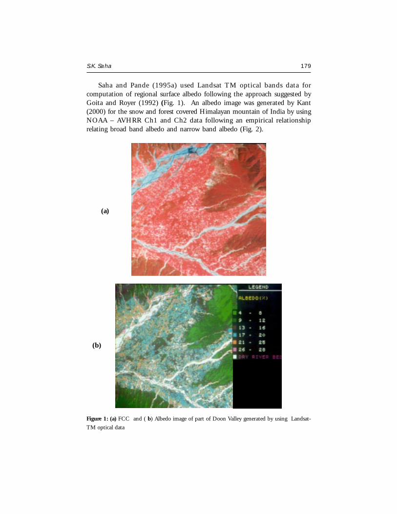
S.K. Saha 179
Saha and Pande (1995a) used Landsat TM optical bands data forcomputation of regional surface albedo following the approach suggested byGoita and Royer (1992) (Fig. 1). An albedo image was generated by Kant(2000) for the snow and forest covered Himalayan mountain of India by usingNOAA – AVHRR Ch1 and Ch2 data following an empirical relationshiprelating broad band albedo and narrow band albedo (Fig. 2).
Figure 1: (a) FCC and ( b) Albedo image of part of Doon Valley generated by using Landsat-
TM optical data
(a)
(b)
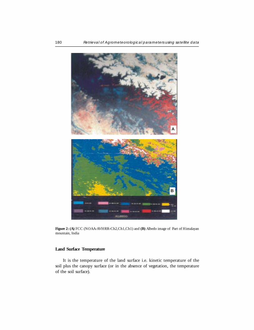
180 Retrieval of Agrometeorological parameters using satellite data
Land Surface Temperature
It is the temperature of the land surface i.e. kinetic temperature of thesoil plus the canopy surface (or in the absence of vegetation, the temperatureof the soil surface).
Figure 2: (A) FCC (NOAA-AVHRR-Ch2,Ch1,Ch1) and (B) Albedo image of Part of Himalayanmountain, India
A
B
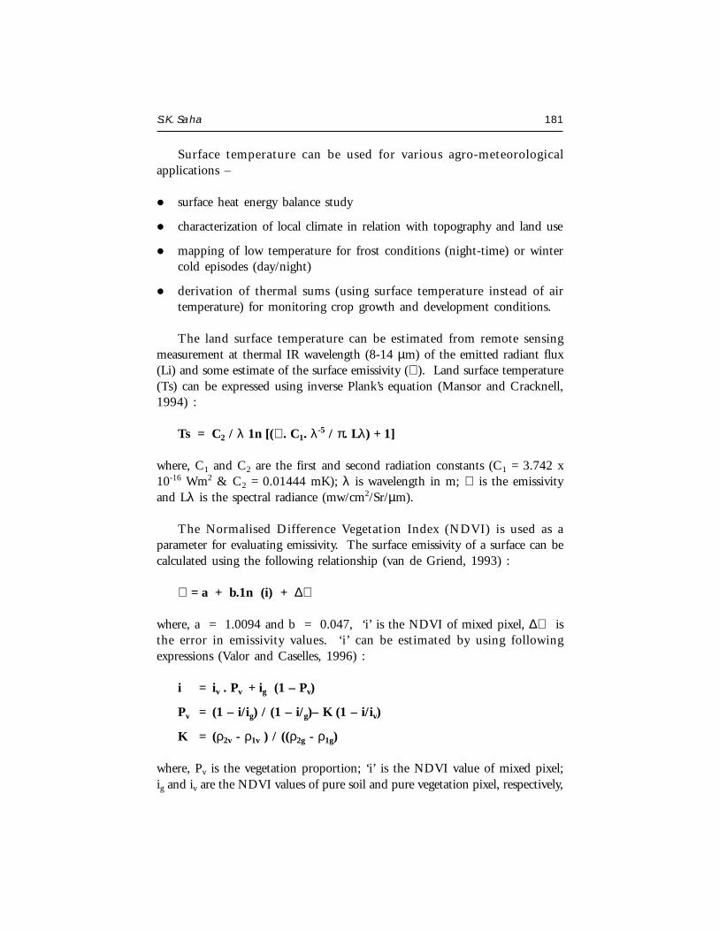
S.K. Saha 181
Surface temperature can be used for various agro-meteorologicalapplications –
surface heat energy balance study
characterization of local climate in relation with topography and land use
mapping of low temperature for frost conditions (night-time) or wintercold episodes (day/night)
derivation of thermal sums (using surface temperature instead of airtemperature) for monitoring crop growth and development conditions.
The land surface temperature can be estimated from remote sensingmeasurement at thermal IR wavelength (8-14 µm) of the emitted radiant flux(Li) and some estimate of the surface emissivity (∈ ). Land surface temperature(Ts) can be expressed using inverse Plank’s equation (Mansor and Cracknell,1994) :
Ts = C2 / λ 1n [(∈ . C1. λ-5 / π. Lλ) + 1]
where, C1 and C2 are the first and second radiation constants (C1 = 3.742 x10⁻¹⁶ Wm2 & C2 = 0.01444 mK); λ is wavelength in m; ∈ is the emissivityand Lλ is the spectral radiance (mw/cm2/Sr/µm).
The Normalised Difference Vegetation Index (NDVI) is used as aparameter for evaluating emissivity. The surface emissivity of a surface can becalculated using the following relationship (van de Griend, 1993) :
∈ = a + b.1n (i) + ∆∈
where, a = 1.0094 and b = 0.047, ‘i’ is the NDVI of mixed pixel, ∆∈ isthe error in emissivity values. ‘i’ can be estimated by using followingexpressions (Valor and Caselles, 1996) :
i = iv . Pv + ig (1 – Pv)
Pv = (1 – i/ig) / (1 – i/g)– K (1 – i/iv)
K = (ρ2v - ρ1v ) / ((ρ2g - ρ1g)
where, Pv is the vegetation proportion; ‘i’ is the NDVI value of mixed pixel;ig and iv are the NDVI values of pure soil and pure vegetation pixel, respectively,
182 Retrieval of Agrometeorological parameters using satellite data
ρ2v and ρ1v are the reflectances in NIR and red region for pure vegetationpixels; ρ2g , ρ1g are the reflectances in NIR and red region for pure soil pixels.
∆∈ = 4 < d∈ > Pv (1 – Pv )
where, ∆∈ is mean weighed value taking into account the different vegetationin the area, their structure and their proportion in it.
The NOAA – AVHRR channels 4 & 5 (10.3 – 10.3 and 11.5 – 12.5µm) are widely used for deriving surface temperature for the day time passes.The temperatures derived from channels 4 and 5 are slightly different due toatmospheric water vapour absorption. Thus, in the land surface retrievalalgorithm, the incorporation of the difference between channels 4 & 5 couldbe useful in correcting for the atmospheric water vapour effect as a first degreeapproximation. An approach based on the differential absorption in twoadjacent infrared channels is called “split-window” technique and is used fordetermination of surface temperature.
In split-window algorithm, brightness temperatures in AVHRR channel4 (T4) and channel 5 (T5), mean emissivity ∈ , i.e. (∈ 4 + ∈ 5)/2; difference inemissivity ∆∈ , i.e. (∈ 4 - ∈ 5), have been used for the estimation of land surfacetemperature using the following relation (Becker and Li, 1990) :
Ts = A + B [(T4 + T5) / 2] + C [ (T4 - T5) / 2]
where, A, B and C are co-efficients worked out by statistical analysis and givenby :
A = 1.274; B = 1 + {0.15616 (1- ∈ ) / ∈ } – 0.482 (∆∈ / ∈ 2)
C = 6.26 + { 3.98 (1- ∈ ) / ∈ } + 38.33 (∆∈ / ∈ 2)
Brightness temperature (TB) values have been calculated by using theinverse of Planck’s radiation equation :
T (B) = C2. V / 1n (1 + C1 . V3 / Ei)
Ei = Si . C + Ii (Kidwell, 1991)
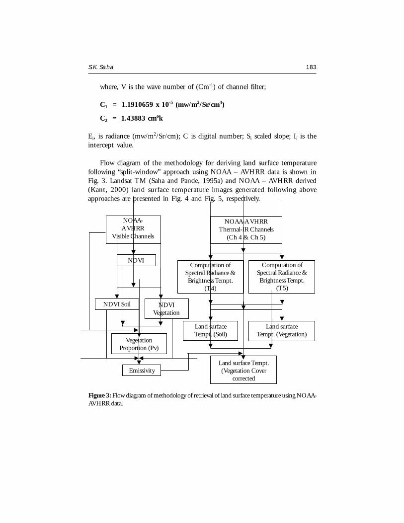
S.K. Saha 183
where, V is the wave number of (Cm-1) of channel filter;
C1 = 1.1910659 x 10⁻⁵ (mw/m2/Sr/cm4)
C2 = 1.43883 cmok
Ei, is radiance (mw/m2/Sr/cm); C is digital number; Si scaled slope; Ii is theintercept value.
Flow diagram of the methodology for deriving land surface temperaturefollowing “split-window” approach using NOAA – AVHRR data is shown inFig. 3. Landsat TM (Saha and Pande, 1995a) and NOAA – AVHRR derived(Kant, 2000) land surface temperature images generated following aboveapproaches are presented in Fig. 4 and Fig. 5, respectively.
Figure 3: Flow diagram of methodology of retrieval of land surface temperature using NOAA-AVHRR data.
NOAA-A VHRR
Visible Channels
NOAA-A VHRRThermal-IR Channels
(Ch 4 & Ch 5)
Computation ofSpectral Radiance &Brightness Tempt.
(T4)
Computation ofSpectral Radiance &Brightness Tempt.
(T5)
Land surfaceTempt. (Vegetation)
Land surfaceTempt. (Soil)
Land surface Tempt.(Vegetation Cover
correctedEmissivity
VegetationProportion (Pv)
NDVIVegetation
NDVI Soil
NDVI
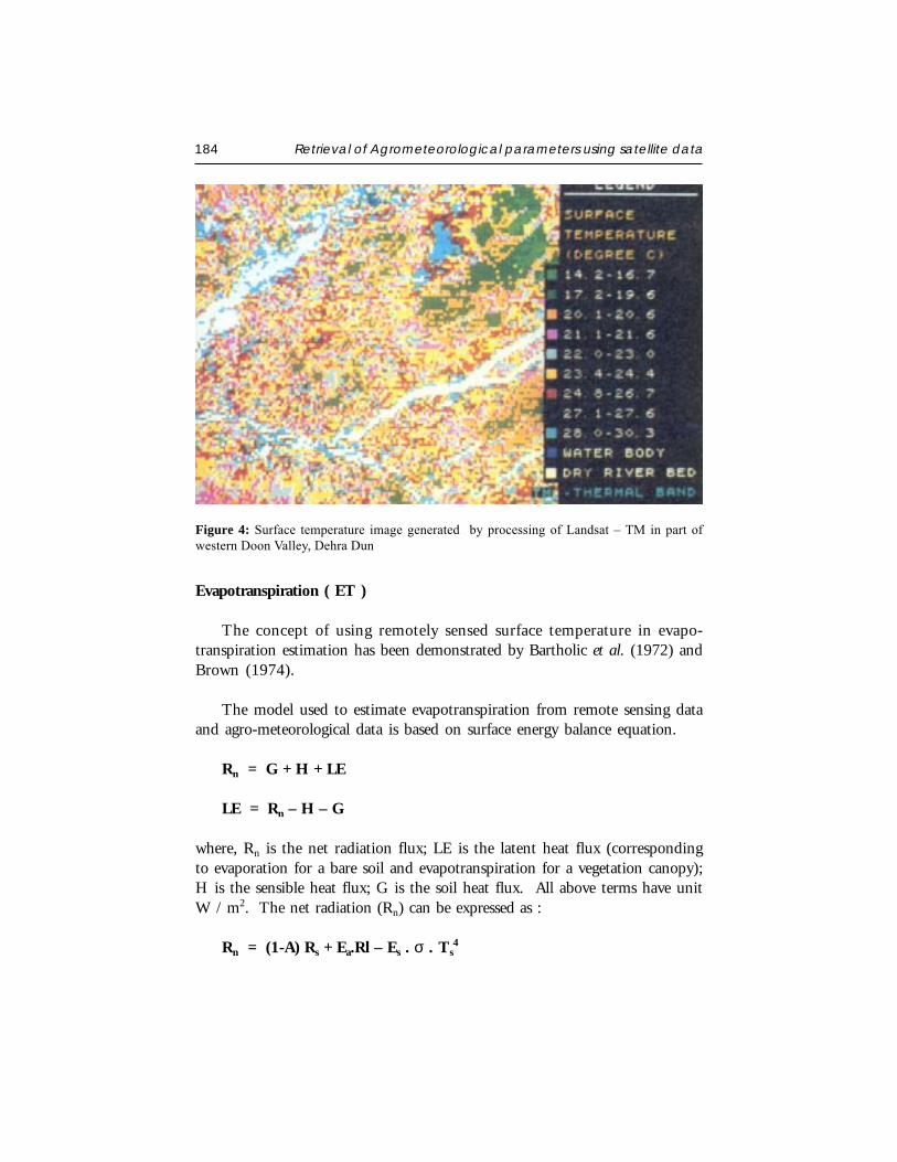
184 Retrieval of Agrometeorological parameters using satellite data
Evapotranspiration ( ET )
The concept of using remotely sensed surface temperature in evapo-transpiration estimation has been demonstrated by Bartholic et al. (1972) andBrown (1974).
The model used to estimate evapotranspiration from remote sensing dataand agro-meteorological data is based on surface energy balance equation.
Rn = G + H + LE
LE = Rn – H – G
where, Rn is the net radiation flux; LE is the latent heat flux (correspondingto evaporation for a bare soil and evapotranspiration for a vegetation canopy);H is the sensible heat flux; G is the soil heat flux. All above terms have unitW / m2. The net radiation (Rn) can be expressed as :
Rn = (1-A) Rs + Ea.Rl – Es . σ . Ts4
Figure 4: Surface temperature image generated by processing of Landsat – TM in part ofwestern Doon Valley, Dehra Dun
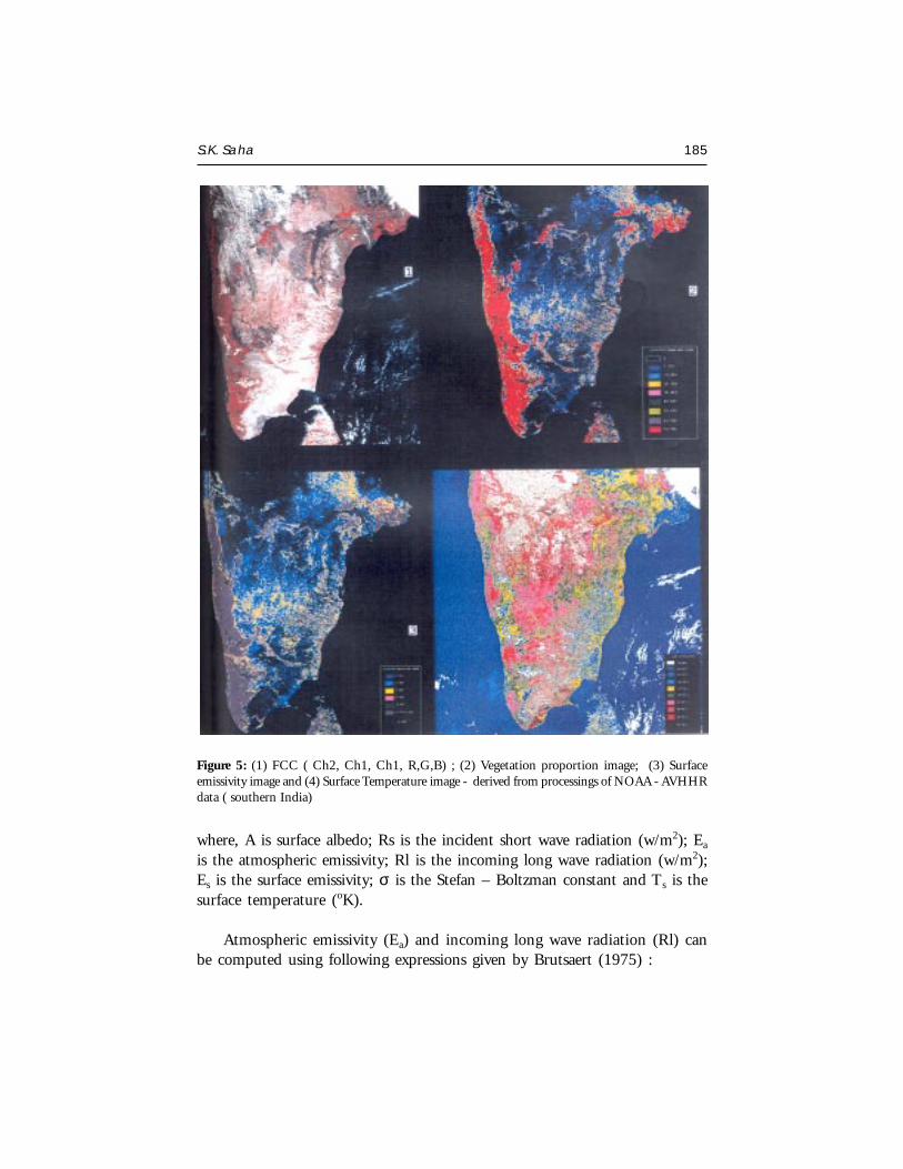
S.K. Saha 185
where, A is surface albedo; Rs is the incident short wave radiation (w/m2); Ea
is the atmospheric emissivity; Rl is the incoming long wave radiation (w/m2);Es is the surface emissivity; σ is the Stefan – Boltzman constant and Ts is thesurface temperature (oK).
Atmospheric emissivity (Ea) and incoming long wave radiation (Rl) canbe computed using following expressions given by Brutsaert (1975) :
Figure 5: (1) FCC ( Ch2, Ch1, Ch1, R,G,B) ; (2) Vegetation proportion image; (3) Surfaceemissivity image and (4) Surface Temperature image - derived from processings of NOAA - AVHHRdata ( southern India)
186 Retrieval of Agrometeorological parameters using satellite data
Ea = 1.24 (ea / Ta)1/7
RL = σ . Ta4
where, ea is the vapour pressure of air at ambient air temperature Ta. Thesensible heat flux may be written as :
H = ρ . Cp (Ts – Ta) / ϒa
where, ρ is the air density; Cp is the specific heat of air, ϒa is the aero-dynamicresistance for sensible heat flux (S/m). The aero-dynamic resistance (ϒa) canbe expressed as (Hatfield et al., 1984) :
UKd)/zo}{(z1
a 2
2nγ −=
where, Z is the reference height (2m); d is the zero plane of displacement(m) ( = 2 h/3 h is the height of vegetation); Zo is the surface roughness height(m) ( = h/8); K is the Von Karman’s constant (≈ 0.38) and U is the windspeed at Z (m/s).
Soil heat flux can be written as function of net radiation (Ma et al., 1999):
Ts (0.003.A + A2) ( 1-0.978 NDVI 4) .Rn G = ——
A (for vegetated surface)
G = 0.20 . Rn (for bare surface )
Since, H, G and Rn are instantaneous, it is necessary to apply a procedureto integrate to daily totals. The evaporative fraction (Brutsaert and Sugita,1992) is the energy used for evaporation process divided by the total amountof energy available for the evaporation process.
GRLE
HLHLH ^
n −=
+=
Although, the H and LE fluctuate strongly on daily basis, the evaporativefraction behaves steady during day time. Then, the link between theinstantaneous and the integrated daily case is given by
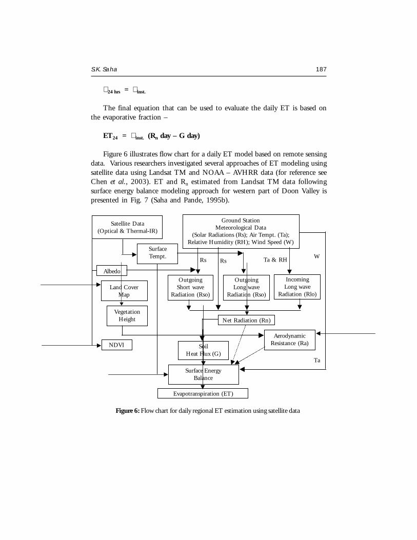
S.K. Saha 187
∧ 24 hrs = ∧ inst.
The final equation that can be used to evaluate the daily ET is based onthe evaporative fraction –
ET24 = ∧ inst. (Rn day – G day)
Figure 6 illustrates flow chart for a daily ET model based on remote sensingdata. Various researchers investigated several approaches of ET modeling usingsatellite data using Landsat TM and NOAA – AVHRR data (for reference seeChen et al., 2003). ET and Rn estimated from Landsat TM data followingsurface energy balance modeling approach for western part of Doon Valley ispresented in Fig. 7 (Saha and Pande, 1995b).
Figure 6: Flow chart for daily regional ET estimation using satellite data
Satellite Data(Optical & Thermal-IR)
Ground StationMeteorological Data
(Solar Radiations (Rs); Air Tempt. (Ta);Relative Humidity (RH); Wind Speed (W)
OutgoingShort wave
Radiation (Rso)
OutgoingLong wave
Radiation (Rso)
IncomingLong wave
Radiation (Rlo)
AerodynamicResistance (Ra)Soil
Heat Flux (G)
Surface EnergyBalance
Evapotranspiration (ET)
SurfaceTempt.
Land CoverMap
VegetationHeight
NDVI
Albedo
Net Radiation (Rn)
W
Ta
Rs Rs Ta & RH

188 Retrieval of Agrometeorological parameters using satellite data
Absorbed Photosynthetically Active Radiation (APAR)
APAR is the fraction of the PAR (Photosynthetically Active Radiation)absorbed by the canopy and used for carbon dioxide assimilation. PAR refersto the visible part of the solar spectrum between 0.4 and 0.7 µm, wherechlorophyll absorbs solar radiation. APAR is a key parameter in productivityanalysis and ecosystem modeling. The productivity of vegetation canopies canbe studied from estimation of APAR derived from optical remote sensing data.
The APAR results from a leaf radiation balance :
APAR = PAR - ppAR . PAR – PARtrans + PARsoil
where, pPAR is the canopy reflectance at the upper side of the canopy in the0.4 to 0.7µm spectral range, PARtrans is the amount of PAR that is transmittedthrough the canopy and directed to the soil; PARsoil that is reflected from thesoil underneath the canopy and is received back at the lower side of the canopy.
APAR can be deduced directly from PAR after simplifying the previousequation into :
Figure 7: Evapotranspiration image of part of western Doon Valley generated by processingof Landsat – TM data
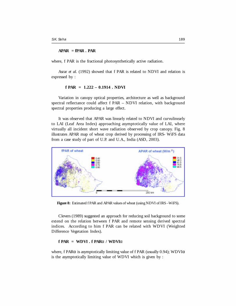
S.K. Saha 189
APAR = fPAR . PAR
where, f PAR is the fractional photosynthetically active radiation.
Asrar et al. (1992) showed that f PAR is related to NDVI and relation isexpressed by :
f PAR = 1.222 – 0.1914 . NDVI
Variation in canopy optical properties, architecture as well as backgroundspectral reflectance could affect f PAR – NDVI relation, with backgroundspectral properties producing a large effect.
It was observed that APAR was linearly related to NDVI and curvulinearlyto LAI (Leaf Area Index) approaching asymptotically value of LAI, wherevirtually all incident short wave radiation observed by crop canopy. Fig. 8illustrates APAR map of wheat crop derived by processing of IRS- WiFS datafrom a case study of part of U.P. and U.A., India (ASD, 2003).
Figure 8: Estimated f PAR and APAR values of wheat (using NDVI of IRS –WiFS).
Clevers (1989) suggested an approach for reducing soil background to someextend on the relation between f PAR and remote sensing derived spectralindices. According to him f PAR can be related with WDVI (WeightedDifference Vegetation Index).
f PAR = WDVI . f PARα / WDVIα
where, f PARα is asymptotically limiting value of f PAR (usually 0.94); WDVIαis the asymptotically limiting value of WDVI which is given by :
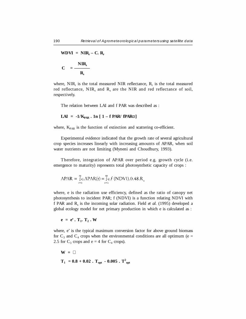
190 Retrieval of Agrometeorological parameters using satellite data
WDVI = NIRr – C. Rr
NIRs
C = –——— Rs
where, NIRr is the total measured NIR reflectance, Rr is the total measuredred reflectance, NIRs and Rs are the NIR and red reflectance of soil,respectively.
The relation between LAI and f PAR was described as :
LAI = -1/KPAR . 1n [ 1 – f PAR/ fPARα]
where, KPAR is the function of extinction and scattering co-efficient.
Experimental evidence indicated that the growth rate of several agriculturalcrop species increases linearly with increasing amounts of APAR, when soilwater nutrients are not limiting (Myneni and Choudhury, 1993).
Therefore, integration of APAR over period e.g. growth cycle (i.e.emergence to maturity) represents total photosynthetic capacity of crops :
where, e is the radiation use efficiency, defined as the ratio of canopy netphotosynthesis to incident PAR; f (NDVI) is a function relating NDVI withf PAR and Rs is the incoming solar radiation. Field et al. (1995) developed aglobal ecology model for net primary production in which e is calculated as :
e = e’ . T1. T2 . W
where, e’ is the typical maximum conversion factor for above ground biomassfor C3 and C4 crops when the environmental conditions are all optimum (e =2.5 for C3 crops and e = 4 for C4 crops).
W = ∧
T1 = 0.8 + 0.02 . Topt - 0.005 . T2opt
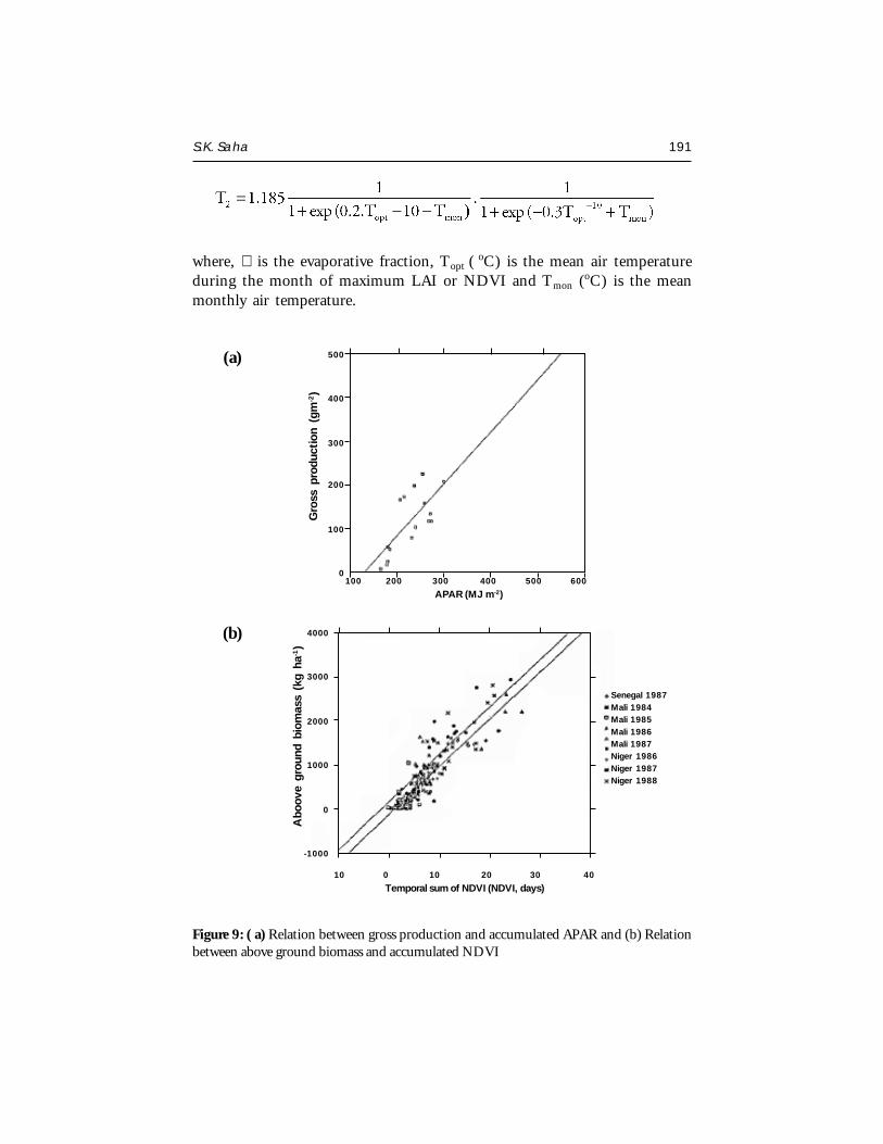
S.K. Saha 191
where, ∧ is the evaporative fraction, Topt ( oC) is the mean air temperature
during the month of maximum LAI or NDVI and Tmon (oC) is the meanmonthly air temperature.
Figure 9: ( a) Relation between gross production and accumulated APAR and (b) Relationbetween above ground biomass and accumulated NDVI
(a)
Gro
ss p
rodu
ctio
n (g
m-2)
500
400
300
200
100
0100 200 300 400 500 600
APAR (MJ m-2)
(b) 4000
3000
2000
1000
0
-1000
Abo
ove
grou
nd b
iom
ass
(kg
ha-1)
10 0 10 20 30 40
Temporal sum of NDVI (NDVI, days)
Senegal 1987Mali 1984Mali 1985Mali 1986Mali 1987Niger 1986Niger 1987Niger 1988
192 Retrieval of Agrometeorological parameters using satellite data
Therefore, temporal sums of NDVI which is giving cumulative values ofAPAR, can be used for estimation of crop/vegetation productivity. Prince(1990) observed a good linear relationship between APAR and vegetation grossproduction and also strong positive relationship between above groundvegetation biomass and temporal sum of NOAA – AVHRR NDVI (Fig. 9)in parts of Africa.
CONCLUSIONS
Remotely sensed satellite optical and thermal infrared can be synergisticallyused to estimate surface agro-meteorological properties. Optical data can beused to estimate land surface albedo by integrating narrow-band directionalspectral reflectances. Thermal IR data from various satellites appear as valuabletool for vegetation growth and conditions assessment by retrieval of land surfacetemperature and estimation of evapotranspiration following various modelingapproaches. Optical data in the form of spectral indices are found to be relatedto solar radiation absorbed by vegetation canopies and this is useful for assessingregional vegetation potential productivity.
REFERENCES
Asrar, G. Myneni, R.B. and Choudhury, B.J. 1992. Spatial heterogeneity in vegetationcanopies and remote sensing of absorbed photosynthetically active radiation : a modelingstudy. Remote Sensing Environment, 41 : 85-103.
Bartholic, J. F., Namken, K.N. and Wiegand, C.L. 1972. Aerial thermal scanner to determinetemperature of soil and crop canopies differing in water stress. Agronomy Journal, 6 :603.
Becker, F. and Li, L. 1990. Towards a local split window method over land surface. RemoteSensing Environment, 32 (17) : 17-33.
Brest, C.L. and Goward, S.N. 1987. Deriving surface albedo from narrow band satellitedata. International Journal of Remote Sensing, 8 : 351-367.
Brown, K.W. 1974. Calculation of evapotranspiration from crop surface temperature.Agricultural Meteorology, 14 : 199-209.
Brutsaert, W. 1975. On a derivable formula of long wave radiation from clear skies. WaterResource Research, 11 : 742 – 744.
S.K. Saha 193
Brutsaert, W. and Sugita 1992. Application of self-preservation in the diurnal evolution ofthe surface energy budget to determine daily evaporation. Journal of Geophysical Research,19 (17) : 18, 377 – 18, 382.
Chen, Y.; Li, X.; Jing, G. and Shi, P. 2003. An estimation model for daily regionalevapotranspiration. International Journal of Remote Sensing, 24 : 199 – 205.
Clevers, J.G.P.W. 1988. A simplified reflectance model for the estimation of Leaf Area Index.Remote Sensing Environment, 25 : 53-69.
Field, C.B.; Randerson, J.J. and Malmstrom, C.M. 1995. Global net primary productivityproduction : Combining ecology and remote sensing. Remote Sensing Environment,51 (1) : 74-88.
Goita, K. and Royer, A. 1992. Land surface climatology and land cover change monitoringsince 1973 over a north-Sahelian zone using Landsat data. Geocarto-International, 2:15-28.
Hatfield, J.L.; Reginato, R.J. and Idso, S.B. 1984. Evaluation of canopy temperatureevapotranspiration models over various crops. Agricultural and Forest Meteorology, 32:41 – 53.
Kant, Yogesh 2000. Studies on Land Surface Process using Satellite Data. Ph.D. Thesis inPhysics, Omania University, India.
Myneni, R.B. and Choudhary, B.J. 1993. Synergistic use of Optical and Microwave datain agro-meteorological applications. Advances in Space Research, 13 (5) : 239-248.
Mansor, S.B. and Cracknell, A.P. 1994. Monitoring of coal fires using thermal infrareddata. International Journal of Remote Sensing, 15 (8) : 1675 – 1685.
Prasad, S.; Gupta, R.K. and Sesa Sai, M.V.R. 1995. Computation of surface albedo fromNOAA – AVHRR data. Pages 51-57. In Proc. National Symposium on Remote SensingEnvironment with special emphasis on Green Revolution. ISRS, India.
Prince, S.D. 1990. High temporal frequency remote sensing of primary production usingNOAA – AVHRR. Pages 169-184. In book “Applications of Remote Sensing inAgriculture” (Eds. M.D. Steven and J.A. Clark). Butterworth.
Saha, S.K. and Pande, L.M.1995a. Regional surface albedo and ET modeling usingcombination of optical and thermal IR data. Pages 70-78. In book “Advances in TropicalMeteorology” (R.K. Dutta, Ed.). Concept Publishers, New Delhi, India.
Saha, S.K. and Pande, L.M.1995b. Modeling land surface energy balance components andassessment of crop water stress – a satellite thermal IR remote sensing approach. Proc.ISRS Silver Jubilee Year Seminar, Dehra Dun.
194 Retrieval of Agrometeorological parameters using satellite data
Saunders, R.W. 1990. In determination of broad band surface albedo from AVHRR visibleand near infrared radiances. International Journal of Remote Sensing, 11 (1) : 49 –67.
Valor, E. and Caselles, V. 1996. Mapping land surface emissivity from NDVI; applicationto European, Africa and South American areas. Remote Sensing Environment, 57 :167 – 184.
van de Gried, A.A. and Owe, M.1993. On the relationship between thermal emissivityand the normalized difference vegetation index for natural surfaces. International Journalof Remote Sensing, 14 : 1119 – 1131.
Valientz, J.A.; Nunez, M.; Lopez – Baeza E. and Poreno, J.F. 1995. Narrow band to broadband conversion for Meteosat – visible channel and broad – band albedo using bothAVHRR –1 and 2 channels. International Journal of Remote Sensing, 16 (6) : 1147 –1166.
RETRIEVAL OF AGROMETEOROLOGICALPARAMETERS FROM SATELLITES
C.M. KishtawalAtmospheric Sciences DivisionMeteorology and Oceanographic GroupSpace Application Centre (ISRO), Ahmedabad
Abstract: In this article the techniques of the retrieval of agro-meteorologicalparameters like cloudiness, rainfall, soil moisture, solar radiation, surfacetemperature, and shelter temperature/humidity using different approaches arediscussed. A discussion is presented on the state-of-the-art sensors, and how theycan be helpful in providing some additional parameters and also, the conventionalparameters (as mentioned above) with better accuracy.
INTRODUCTION
Satellites offer a unique source of information for many agriculturalapplications. Among their attributes are: (1) regular, repetitive observationpatterns; (2) large scale synoptic view of the earth surface from space; and (3)availability of a permanent information archive for establishing baseline data.In the following sections a brief outline of the weather parameters of agro-meteorological importance is provided, and a discussion about the usefulnessof satellite observations in the retrieval of these parameters is given.
PARAMETERS OF AGRO-METEOROLOGICAL INTEREST
Although a large number of atmospheric parameters can affect theagricultural production in short and long time scale, we will confine the currentdiscussion to a few parameters. Also, we will see how the satellite observationscan play a role in determination of these parameters. The parameters discussedin the following subsections are:
Satellite Remote Sensing and GIS Applications in Agricultural Meteorologypp. 195-211
196 Retrieval of Agrometeorological Parameters from Satellites
Clouds
Rainfall
Soil Moisture
Solar Radiation
Surface Temperature
Temperature and Humidity Profiles.
Meteorological satellites play an important role in retrieval of the aboveparameters at large spatial scales. The following subsections provide thediscussion on this aspect.
Clouds
Interpretation of Cloud in Visible/Infrared Imageries
The cloud configuration seen in satellite imagery represents a visiblemanifestation of all types of atmospheric processes. The complete interpretationof cloud structure must make use of both satellite imagery and other availableobservational data. One should remember that the satellite sensors view onlytops of clouds while in surface observations their bases are seen. Basicallyfollowing six characteristic features of satellite pictures are helpful in extractinginformation for weather forecasting:
i) Brightness - The brightness depends strongly upon the albedo of theunderlying surface in visible pictures. Highly reflecting surfaces likecumulonimbus (Cb) tops and snow appear pure white whereas the sealooks black. Other clouds and land appear in varying degrees of gray. InIR images warm land surfaces appear very dark while cold ones are white(e.g. Cb tops, thick cirrus, snow etc.). Lower level clouds and thin cirrusappear gray.
ii) Pattern - Cloud elements are seen to be organised into identifiable patternslike lines, bands, waves etc.
iii) Structure - In a VIS image, shadows of taller clouds fall on lower surfaces.Shadows and highlights thus give an idea of the cloud structure. In IR
C.M. Kishtawal 197
imagery this information is provided by the cloud top temperature (CTT)more directly.
iv) Texture - The cloud surfaces when viewed by the satellite vary in degreeof apparent smoothness. Some clouds appear smooth while some may lookragged.
v) Shape - Clouds assume a variety of shapes - rounded, straight, serrated,scalloped, diffused or curved.
vi) Size - The size of a pattern or the size of individual elements in a patternare useful indicators of the scale of weather systems.
While interpreting satellite pictures continuity in time has to bemaintained. The pictures should not be viewed in isolation but must beinterpreted with reference to past weather and earlier imageries. It is necessaryto keep in mind the time of the day, season and local peculiarities whileinterpreting satellite imageries. In VIS pictures illumination depends on theposition of the sun which will vary the brightness of clouds. Similarly indifferent seasons (e.g. summer and winter) the image disc of the northern andsouthern hemisphere will have different brightness. Local features likemountains and valleys introduce their own effects. In IR imagery elevated landlike Tibetan Plateau will be cold at night and would appear very bright whereastropical oceans would maintain about the same gray shade throughout thediurnal cycle.
Interpretation of Visible Imageries
Clouds have higher albedo than land (apart from snow cover) and appearwhite or light grey in a VIS imagery. Their brightness depends on theirphysical properties. Clouds with high albedo have large depth, high cloudwater (ice) content, small cloud-droplet size whereas clouds with low albedohave shallow depth, low cloud water (ice) content, large average cloud-dropletsize. The water content and depth of the cloud are the most important. TypicalAlbedo values are given in Table 1.
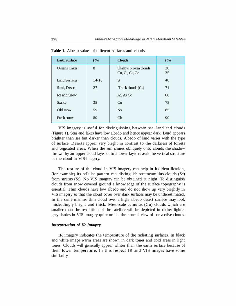
198 Retrieval of Agrometeorological Parameters from Satellites
Table 1. Albedo values of different surfaces and clouds
Earth surface (%) Clouds (%)
Oceans, Lakes 8 Shallow broken clouds 30Cu, Ci, Cs, Cc 35
Land Surfaces 14-18 St 40
Sand, Desert 27 Thick clouds (Cs) 74
Ice and Snow Ac, As, Sc 68
Sea ice 35 Cu 75
Old snow 59 Ns 85
Fresh snow 80 Cb 90
VIS imagery is useful for distinguishing between sea, land and clouds(Figure 1). Seas and lakes have low albedo and hence appear dark. Land appearsbrighter than sea but darker than clouds. Albedo of land varies with the typeof surface. Deserts appear very bright in contrast to the darkness of forestsand vegetated areas. When the sun shines obliquely onto clouds the shadowthrown by an upper cloud layer onto a lower layer reveals the vertical structureof the cloud in VIS imagery.
The texture of the cloud in VIS imagery can help in its identification,(for example) its cellular pattern can distinguish stratocumulus clouds (Sc)from stratus (St). No VIS imagery can be obtained at night. To distinguishclouds from snow covered ground a knowledge of the surface topography isessential. Thin clouds have low albedo and do not show up very brightly inVIS imagery so that the cloud cover over dark surfaces may be underestimated.In the same manner thin cloud over a high albedo desert surface may lookmisleadingly bright and thick. Mesoscale cumulus (Cu) clouds which aresmaller than the resolution of the satellite will be depicted in rather lightergrey shades in VIS imagery quite unlike the normal view of convective clouds.
Interpretation of IR Imagery
IR imagery indicates the temperature of the radiating surfaces. In blackand white image warm areas are shown in dark tones and cold areas in lighttones. Clouds will generally appear whiter than the earth surface because oftheir lower temperature. In this respect IR and VIS images have somesimilarity.
C.M. Kishtawal 199
Because cloud top temperature decreases with height IR images show goodcontrast between clouds at different levels. This is not possible in VIS imagery.
Coast lines show up clearly in IR images whenever there is strong contrastbetween land and sea surface temperatures. During the day the land mayappear darker (warmer) than the sea but at night may appear lighter (cooler).At times when land and sea temperatures are almost same, it becomesimpossible to detect coastlines in IR imagery. The most marked contrastbetween land and sea is normally found in Summer and Winter and is leastin Spring and Autumn. Thin Ci which is often transparent in the VIS canshow up clearly in IR especially when it lies over much warmer surface.
IR imagery is inferior to VIS in providing information about cloud textureas it is based upon emitted and not scattered radiation. Low clouds and fogcan rarely be observed in IR at night because they have almost the sametemperature as the underlying surface. But during day, such clouds are easilydetected in.
Interpretation of WV Imagery
Water vapor imagery is derived from radiation at wavelengths around 6-7µm. Though this is not an atmospheric window, it is part of the spectrumwhere water vapor is the dominant absorbing gas. It has a strong absorptionband centered on 6.7 µm. In regions of strong absorption, most of the radiationreaching the satellite originates high in the atmosphere. The stronger theabsorption, the higher is the originating level of the emission that ultimatelyreaches the satellite. As the Relative Humidity (RH) decreases the maincontribution of the radiance received by the satellite comes from lower in thetroposphere.
WV imagery is usually displayed with the emitted radiation converted totemperature like IR imagery. Regions of high upper tropospheric humidityappear cold (bright) and regions of low humidity appear warm (dark) i.e. whenthe upper troposphere is dry, the radiation reaching the satellite originatesfrom farther down in the atmosphere where it is warmer and appears darkeron the image. In a normally moist atmosphere most of the WV radiationreceived by the satellite originates in the 300-600 hPa layer. But when theair is dry some radiation may come from layers as low as 800 hPa. Due to thegeneral poleward decrease of water vapor content, the height of thecontributing layer gets lower and lower towards the poles.
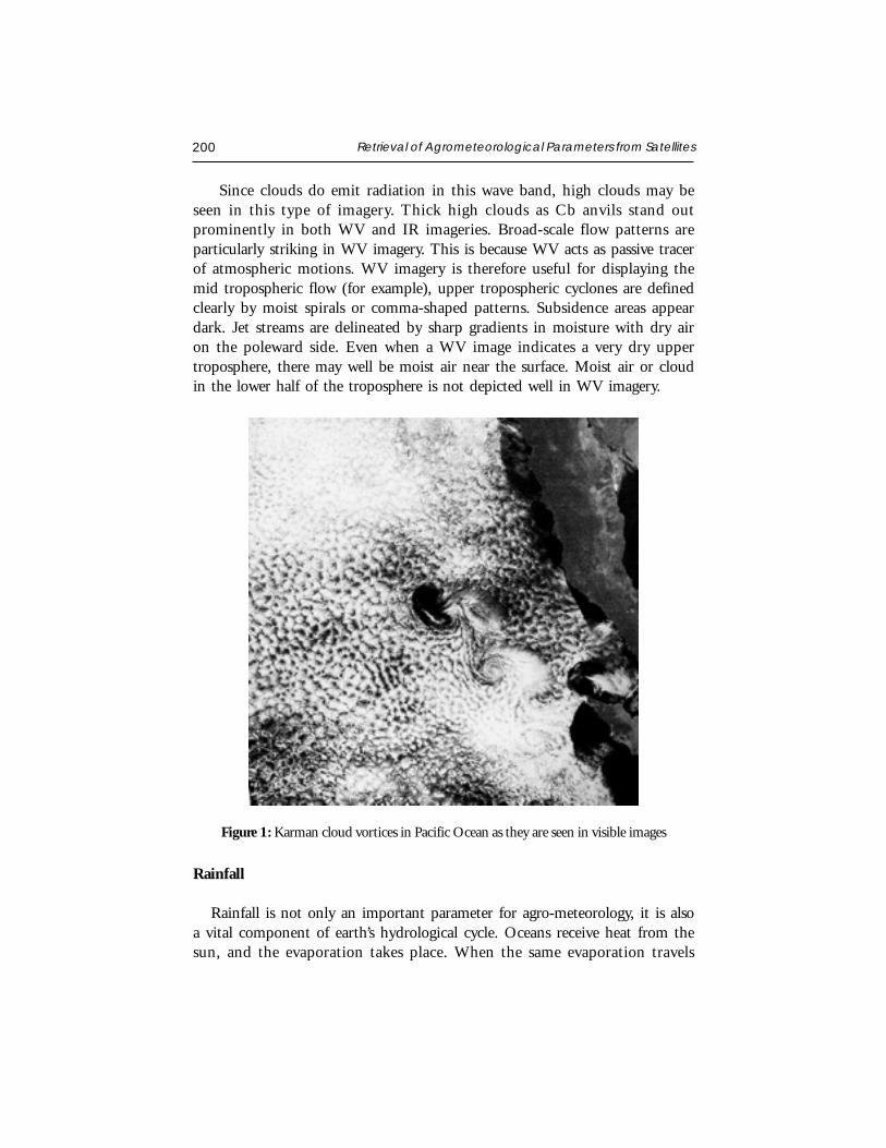
200 Retrieval of Agrometeorological Parameters from Satellites
Since clouds do emit radiation in this wave band, high clouds may beseen in this type of imagery. Thick high clouds as Cb anvils stand outprominently in both WV and IR imageries. Broad-scale flow patterns areparticularly striking in WV imagery. This is because WV acts as passive tracerof atmospheric motions. WV imagery is therefore useful for displaying themid tropospheric flow (for example), upper tropospheric cyclones are definedclearly by moist spirals or comma-shaped patterns. Subsidence areas appeardark. Jet streams are delineated by sharp gradients in moisture with dry airon the poleward side. Even when a WV image indicates a very dry uppertroposphere, there may well be moist air near the surface. Moist air or cloudin the lower half of the troposphere is not depicted well in WV imagery.
Figure 1: Karman cloud vortices in Pacific Ocean as they are seen in visible images
Rainfall
Rainfall is not only an important parameter for agro-meteorology, it is alsoa vital component of earth’s hydrological cycle. Oceans receive heat from thesun, and the evaporation takes place. When the same evaporation travels
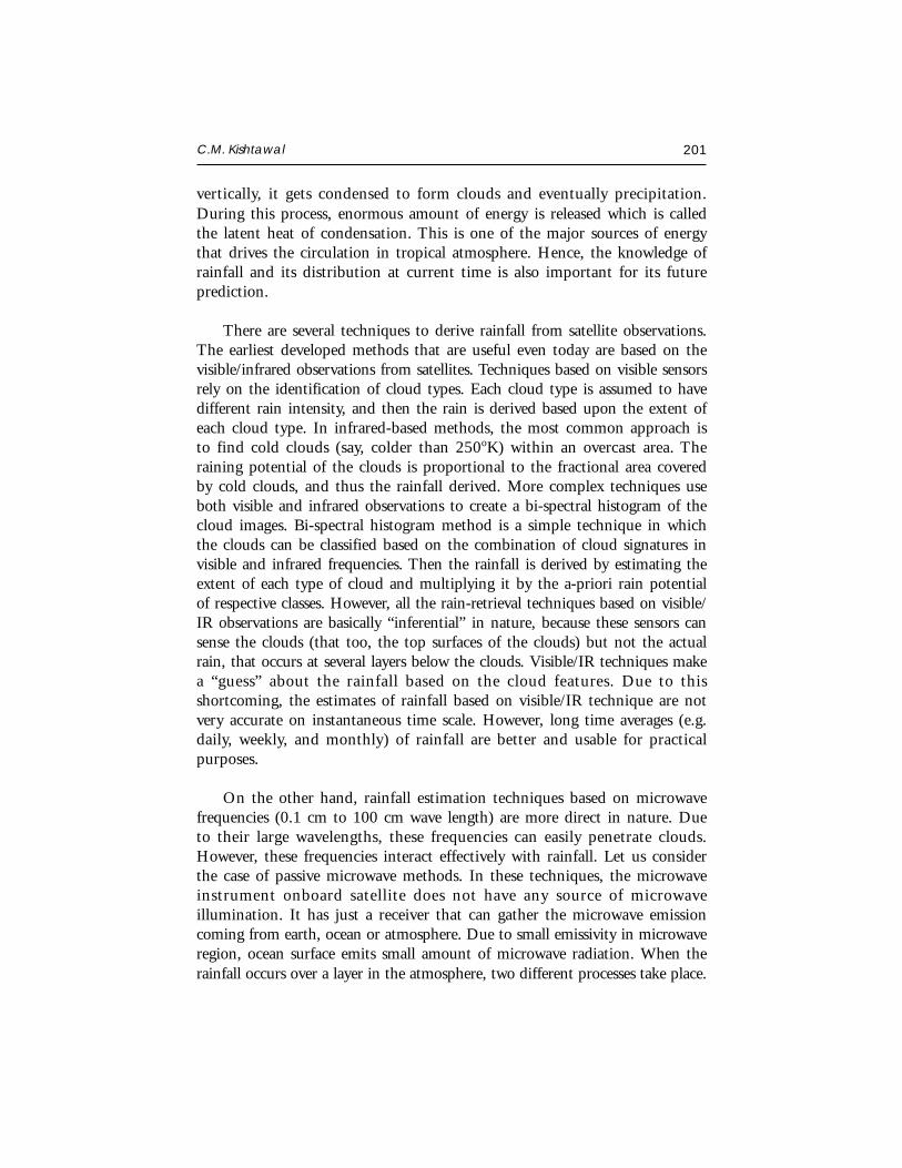
C.M. Kishtawal 201
vertically, it gets condensed to form clouds and eventually precipitation.During this process, enormous amount of energy is released which is calledthe latent heat of condensation. This is one of the major sources of energythat drives the circulation in tropical atmosphere. Hence, the knowledge ofrainfall and its distribution at current time is also important for its futureprediction.
There are several techniques to derive rainfall from satellite observations.The earliest developed methods that are useful even today are based on thevisible/infrared observations from satellites. Techniques based on visible sensorsrely on the identification of cloud types. Each cloud type is assumed to havedifferent rain intensity, and then the rain is derived based upon the extent ofeach cloud type. In infrared-based methods, the most common approach isto find cold clouds (say, colder than 250oK) within an overcast area. Theraining potential of the clouds is proportional to the fractional area coveredby cold clouds, and thus the rainfall derived. More complex techniques useboth visible and infrared observations to create a bi-spectral histogram of thecloud images. Bi-spectral histogram method is a simple technique in whichthe clouds can be classified based on the combination of cloud signatures invisible and infrared frequencies. Then the rainfall is derived by estimating theextent of each type of cloud and multiplying it by the a-priori rain potentialof respective classes. However, all the rain-retrieval techniques based on visible/IR observations are basically “inferential” in nature, because these sensors cansense the clouds (that too, the top surfaces of the clouds) but not the actualrain, that occurs at several layers below the clouds. Visible/IR techniques makea “guess” about the rainfall based on the cloud features. Due to thisshortcoming, the estimates of rainfall based on visible/IR technique are notvery accurate on instantaneous time scale. However, long time averages (e.g.daily, weekly, and monthly) of rainfall are better and usable for practicalpurposes.
On the other hand, rainfall estimation techniques based on microwavefrequencies (0.1 cm to 100 cm wave length) are more direct in nature. Dueto their large wavelengths, these frequencies can easily penetrate clouds.However, these frequencies interact effectively with rainfall. Let us considerthe case of passive microwave methods. In these techniques, the microwaveinstrument onboard satellite does not have any source of microwaveillumination. It has just a receiver that can gather the microwave emissioncoming from earth, ocean or atmosphere. Due to small emissivity in microwaveregion, ocean surface emits small amount of microwave radiation. When therainfall occurs over a layer in the atmosphere, two different processes take place.
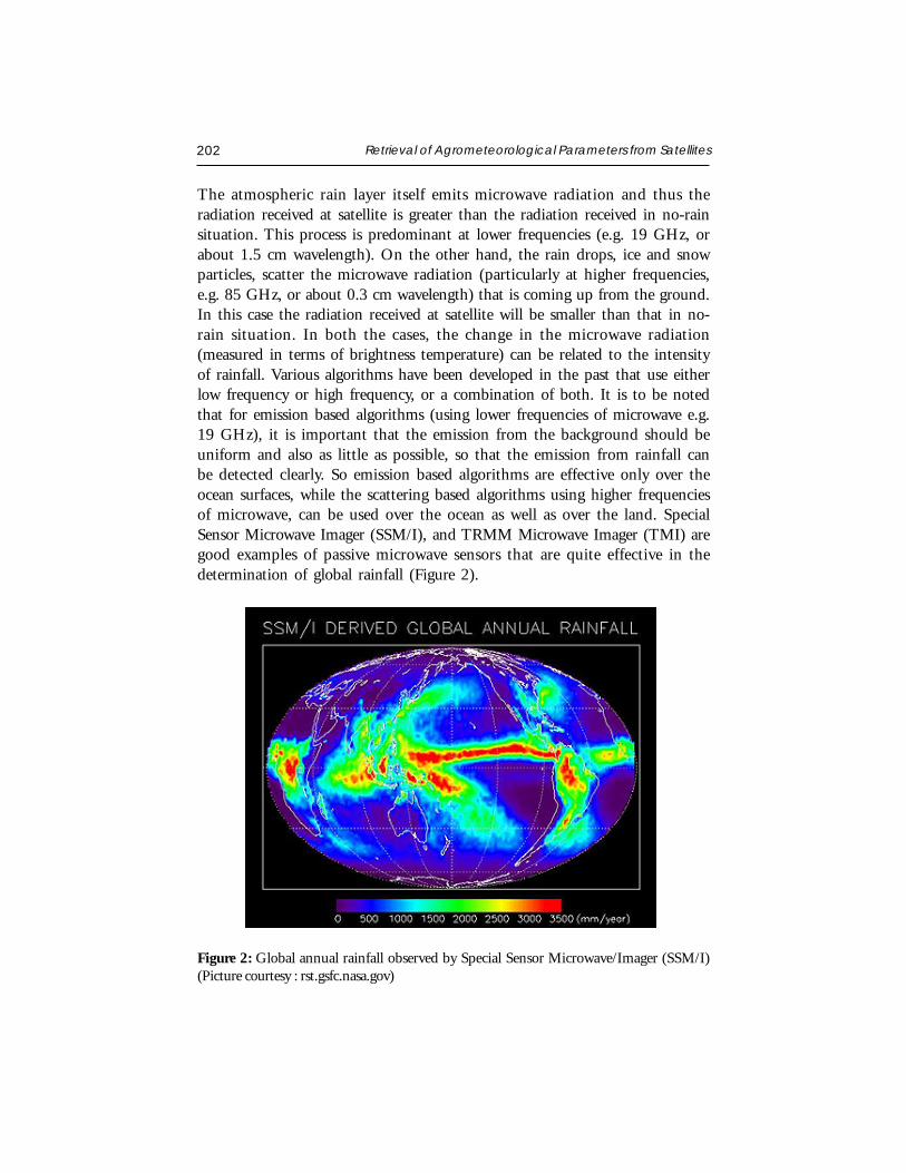
202 Retrieval of Agrometeorological Parameters from Satellites
The atmospheric rain layer itself emits microwave radiation and thus theradiation received at satellite is greater than the radiation received in no-rainsituation. This process is predominant at lower frequencies (e.g. 19 GHz, orabout 1.5 cm wavelength). On the other hand, the rain drops, ice and snowparticles, scatter the microwave radiation (particularly at higher frequencies,e.g. 85 GHz, or about 0.3 cm wavelength) that is coming up from the ground.In this case the radiation received at satellite will be smaller than that in no-rain situation. In both the cases, the change in the microwave radiation(measured in terms of brightness temperature) can be related to the intensityof rainfall. Various algorithms have been developed in the past that use eitherlow frequency or high frequency, or a combination of both. It is to be notedthat for emission based algorithms (using lower frequencies of microwave e.g.19 GHz), it is important that the emission from the background should beuniform and also as little as possible, so that the emission from rainfall canbe detected clearly. So emission based algorithms are effective only over theocean surfaces, while the scattering based algorithms using higher frequenciesof microwave, can be used over the ocean as well as over the land. SpecialSensor Microwave Imager (SSM/I), and TRMM Microwave Imager (TMI) aregood examples of passive microwave sensors that are quite effective in thedetermination of global rainfall (Figure 2).
Figure 2: Global annual rainfall observed by Special Sensor Microwave/Imager (SSM/I)(Picture courtesy : rst.gsfc.nasa.gov)
C.M. Kishtawal 203
Soil Moisture
Recent advances in remote sensing have shown that soil moisture can bemeasured by a variety of techniques. However, only microwave technology hasdemonstrated a quantitative ability to measure soil moisture under a varietyof topographic and vegetation cover conditions so that it could be extendedto routine measurements from a satellite system. Both active and passivemicrowave techniques have been applied by researchers for the estimation ofsoil moisture. Two material properties provide clues about composition andsurface state by the manner in which these attributes interact with themicrowave radiation. One property is the dielectric constant (its symbol isthe small Greek letter, k), which is the ratio of the capacitance of a materialto that of a vacuum. It is a dimensionless number that is set at 1.00. Thiselectrical property describes a material’s capability (capacity) to hold a charge,which also measures its ability to polarize when subjected to an electric field.Microwave radiation penetrates deeper into materials with low dielectricconstants and reflect more efficiently from those with high constants. Valuesfor k range from 3 to 16 for most dry rocks and soils, and up to 80 for waterwith impurities. Moist soils have values typically between 30 and 60. Thus,variation in emitted microwave radiances (in case of passive microwaveobservations e.g. by radiometers) or reflected-pulse intensities (in case of activemicrowave observations e.g. by radar) may indicate differences in soil moisture,other factors being constant. Dry soil has a high emittance; water surfaces havelow emittance in microwave region. If one adds water to the soil, the emittancefalls and becomes polarized. With the knowledge of “normal” emittance at aparticular location (which depends upon soil type and vegetation), microwaveobservations can be used to detect changes in emittance and therefore of soilmoisture. Since the soil moisture is changed by precipitation, these emittancechanges between two satellite passes can serve as a proxy of precipitation,known as Antecedent Precipitation Index (API).
The second material property is roughness that can be used to define thesoil texture. Materials differ from one another in their natural or cultivatedstate of surface roughness. Roughness, in this sense, refers to minuteirregularities that relate either to textures of the surfaces or of objects on them(such as, closely-spaced vegetation that may have a variety of shapes). Examplesinclude the textural character of pitted materials, granular soils, gravel, grassblades, and other covering objects whose surfaces have dimensional variabilityon the order of millimeters to centimeters. The height of an irregularity,together with radar wavelength and grazing angle at the point of contact,
204 Retrieval of Agrometeorological Parameters from Satellites
determines the behavior of a surface as smooth (specular reflector), intermediate,or rough (diffuse reflector). A surface with an irregularity height averaging 0.5cm will reflect Ka band (l= 0.85 cm), X band (l= 3 cm), and L band (l= 25cm) radar waves as if it were a smooth, intermediate, and rough surface,respectively. Other average heights produce different responses, fromcombinations of “all smooth” to “all rough” for the several bands used. Thissituation means radar, broadcasting three bands simultaneously in a quasi-multi-spectral mode, can produce color composites, if we assign a color toeach band. Patterns of relative intensities for images made from different bandsmay serve as diagnostic tonal signatures for diverse materials whose surfacesshow contrasted roughness.
Solar Radiation
Incoming solar radiation is the primary source of energy for plantphotosynthesis. Solar radiation also plays a key role in evapotranspiration.Visible observations from satellites provide an excellent source of informationabout the amount of solar radiation reaching the plant canopy. A measurementof solar energy reflected to space from earth-atmosphere system immediatelyspecifies the maximum amount of solar energy that can be absorbed at thesurface. Incoming solar radiation can be known by adjusting the amountabsorbed. Hence, for the computation of downwelling solar radiation, thealbedo of the surface must be known. This is especially important over theregions of high reflectivity such as snow and desert. Tarpley (1979) used astatistical regression technique to obtain surface fluxes over the land fromVisible channel observations from geostationary satellites. In this model, cloudamount is estimated for a given location from satellite visible data. Threeseparate regression equations are then used to estimate solar radiation for threecategories of clouds. This method provides an accuracy of 10% for clear sky,30% for partly cloudy and 50% for overcast conditions. Other algorithmslike those by Moser and Raschke (1984), and Pinker and Ewing (1985) usedphysical approaches, and treated the interaction of incoming and reflected solarradiation with the atmosphere and land surfaces in physical manner. Thetransmittance of solar radiation in these approaches is solved by the use ofradiative transfer equations that take into account the concentration profileof different atmospheric components. These physical schemes also take intoaccount the cloudiness and atmospheric water vapor. These methods providerelatively higher accuracy. However, statistical techniques have remained thechoice for operational use. These methods require coincident satellite and
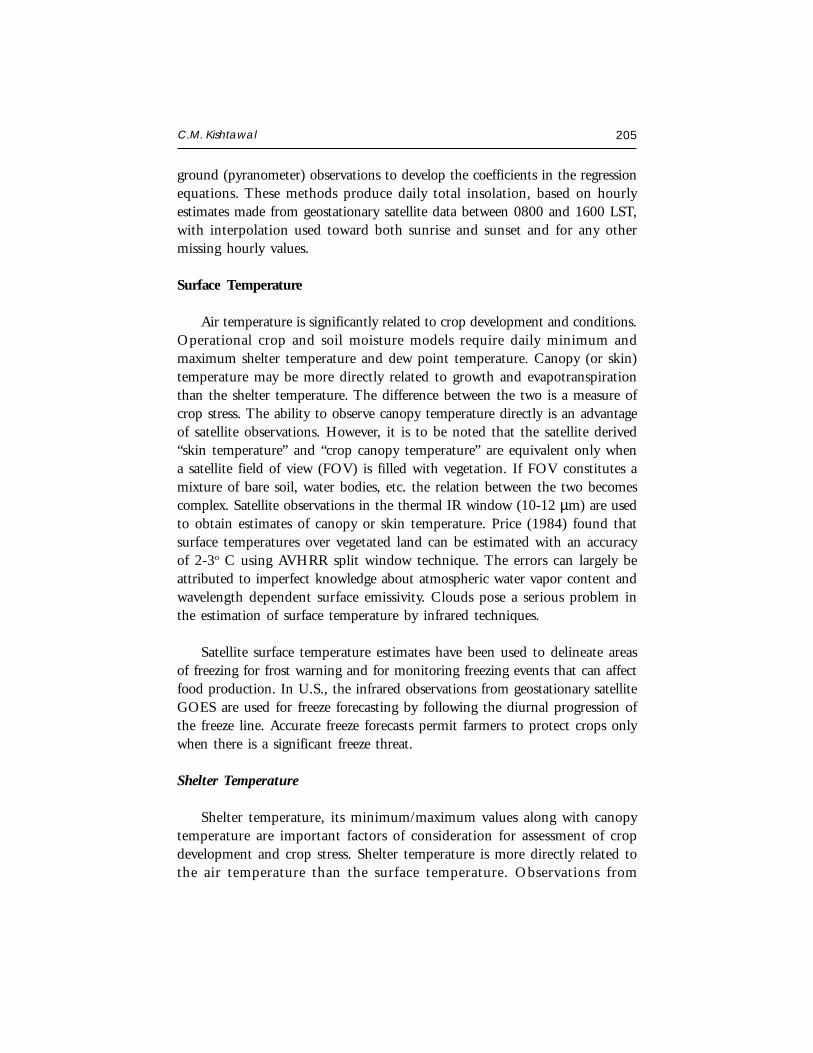
C.M. Kishtawal 205
ground (pyranometer) observations to develop the coefficients in the regressionequations. These methods produce daily total insolation, based on hourlyestimates made from geostationary satellite data between 0800 and 1600 LST,with interpolation used toward both sunrise and sunset and for any othermissing hourly values.
Surface Temperature
Air temperature is significantly related to crop development and conditions.Operational crop and soil moisture models require daily minimum andmaximum shelter temperature and dew point temperature. Canopy (or skin)temperature may be more directly related to growth and evapotranspirationthan the shelter temperature. The difference between the two is a measure ofcrop stress. The ability to observe canopy temperature directly is an advantageof satellite observations. However, it is to be noted that the satellite derived“skin temperature” and “crop canopy temperature” are equivalent only whena satellite field of view (FOV) is filled with vegetation. If FOV constitutes amixture of bare soil, water bodies, etc. the relation between the two becomescomplex. Satellite observations in the thermal IR window (10-12 µm) are usedto obtain estimates of canopy or skin temperature. Price (1984) found thatsurface temperatures over vegetated land can be estimated with an accuracyof 2-3o C using AVHRR split window technique. The errors can largely beattributed to imperfect knowledge about atmospheric water vapor content andwavelength dependent surface emissivity. Clouds pose a serious problem inthe estimation of surface temperature by infrared techniques.
Satellite surface temperature estimates have been used to delineate areasof freezing for frost warning and for monitoring freezing events that can affectfood production. In U.S., the infrared observations from geostationary satelliteGOES are used for freeze forecasting by following the diurnal progression ofthe freeze line. Accurate freeze forecasts permit farmers to protect crops onlywhen there is a significant freeze threat.
Shelter Temperature
Shelter temperature, its minimum/maximum values along with canopytemperature are important factors of consideration for assessment of cropdevelopment and crop stress. Shelter temperature is more directly related tothe air temperature than the surface temperature. Observations from
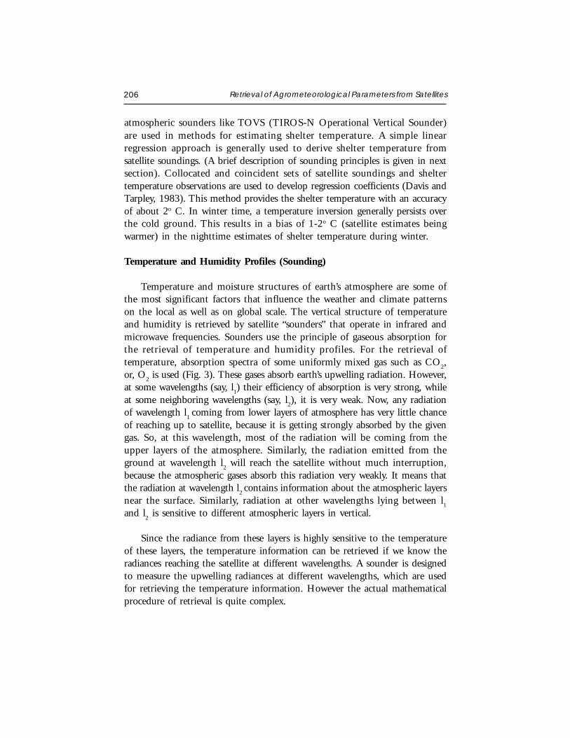
206 Retrieval of Agrometeorological Parameters from Satellites
atmospheric sounders like TOVS (TIROS-N Operational Vertical Sounder)are used in methods for estimating shelter temperature. A simple linearregression approach is generally used to derive shelter temperature fromsatellite soundings. (A brief description of sounding principles is given in nextsection). Collocated and coincident sets of satellite soundings and sheltertemperature observations are used to develop regression coefficients (Davis andTarpley, 1983). This method provides the shelter temperature with an accuracyof about 2o C. In winter time, a temperature inversion generally persists overthe cold ground. This results in a bias of 1-2o C (satellite estimates beingwarmer) in the nighttime estimates of shelter temperature during winter.
Temperature and Humidity Profiles (Sounding)
Temperature and moisture structures of earth’s atmosphere are some ofthe most significant factors that influence the weather and climate patternson the local as well as on global scale. The vertical structure of temperatureand humidity is retrieved by satellite “sounders” that operate in infrared andmicrowave frequencies. Sounders use the principle of gaseous absorption forthe retrieval of temperature and humidity profiles. For the retrieval oftemperature, absorption spectra of some uniformly mixed gas such as CO
2,
or, O2 is used (Fig. 3). These gases absorb earth’s upwelling radiation. However,
at some wavelengths (say, l1) their efficiency of absorption is very strong, while
at some neighboring wavelengths (say, l2), it is very weak. Now, any radiation
of wavelength l1 coming from lower layers of atmosphere has very little chance
of reaching up to satellite, because it is getting strongly absorbed by the givengas. So, at this wavelength, most of the radiation will be coming from theupper layers of the atmosphere. Similarly, the radiation emitted from theground at wavelength l
2 will reach the satellite without much interruption,
because the atmospheric gases absorb this radiation very weakly. It means thatthe radiation at wavelength l
2 contains information about the atmospheric layers
near the surface. Similarly, radiation at other wavelengths lying between l1
and l2 is sensitive to different atmospheric layers in vertical.
Since the radiance from these layers is highly sensitive to the temperatureof these layers, the temperature information can be retrieved if we know theradiances reaching the satellite at different wavelengths. A sounder is designedto measure the upwelling radiances at different wavelengths, which are usedfor retrieving the temperature information. However the actual mathematicalprocedure of retrieval is quite complex.
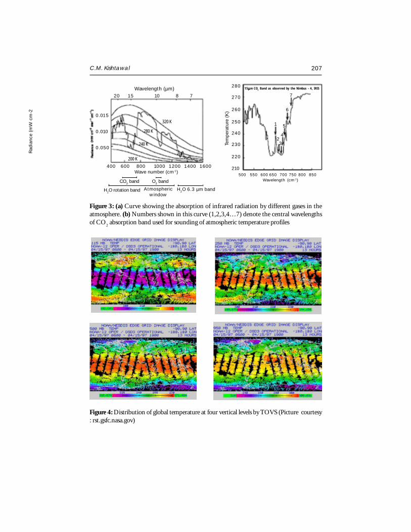
C.M. Kishtawal 207
Figure 3: (a) Curve showing the absorption of infrared radiation by different gases in theatmosphere. (b) Numbers shown in this curve (1,2,3,4…7) denote the central wavelengthsof CO
2 absorption band used for sounding of atmospheric temperature profiles
Figure 4: Distribution of global temperature at four vertical levels by TOVS (Picture courtesy: rst.gsfc.nasa.gov)
CO2 band O2 band
Wave number (cm-1)
H2O rotation band Atmosphericwindow
H2O 6.3 µm band
400 600 800 1000 1200 1400 1600
Rad
ianc
e (m
W c
m-2
320 K
280 K
240 K
200 K
Wavelength (µm)20 15 10 8 7
15µµµµµm CO2 Band as observed by the Nimbus - 4, IRIS280
270
260
250
240
230
220
210500 550 600 650 700 750 800 850
Wavelength (cm-1)
Tem
pera
ture
(K
)
7
6
5
4
1
23
0.015
0.010
0.050
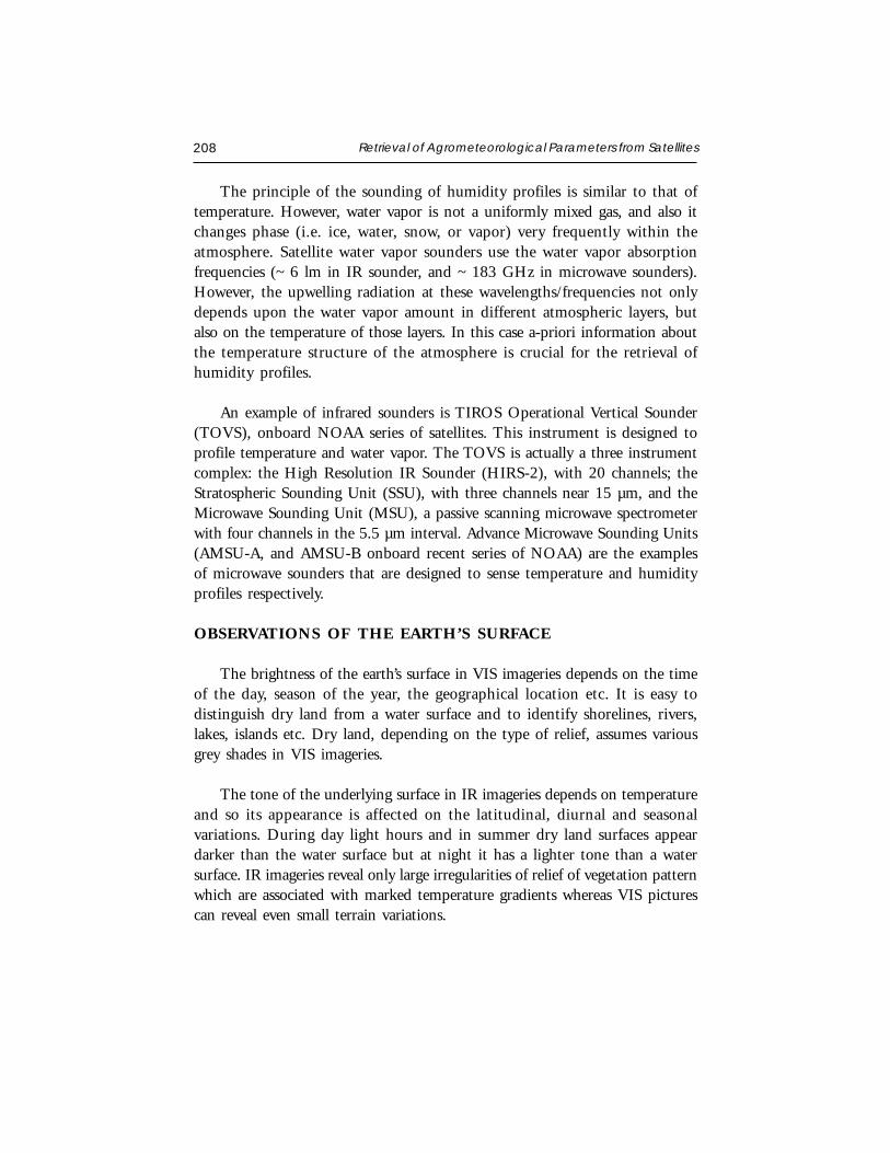
208 Retrieval of Agrometeorological Parameters from Satellites
The principle of the sounding of humidity profiles is similar to that oftemperature. However, water vapor is not a uniformly mixed gas, and also itchanges phase (i.e. ice, water, snow, or vapor) very frequently within theatmosphere. Satellite water vapor sounders use the water vapor absorptionfrequencies (~ 6 lm in IR sounder, and ~ 183 GHz in microwave sounders).However, the upwelling radiation at these wavelengths/frequencies not onlydepends upon the water vapor amount in different atmospheric layers, butalso on the temperature of those layers. In this case a-priori information aboutthe temperature structure of the atmosphere is crucial for the retrieval ofhumidity profiles.
An example of infrared sounders is TIROS Operational Vertical Sounder(TOVS), onboard NOAA series of satellites. This instrument is designed toprofile temperature and water vapor. The TOVS is actually a three instrumentcomplex: the High Resolution IR Sounder (HIRS-2), with 20 channels; theStratospheric Sounding Unit (SSU), with three channels near 15 µm, and theMicrowave Sounding Unit (MSU), a passive scanning microwave spectrometerwith four channels in the 5.5 µm interval. Advance Microwave Sounding Units(AMSU-A, and AMSU-B onboard recent series of NOAA) are the examplesof microwave sounders that are designed to sense temperature and humidityprofiles respectively.
OBSERVATIONS OF THE EARTH’S SURFACE
The brightness of the earth’s surface in VIS imageries depends on the timeof the day, season of the year, the geographical location etc. It is easy todistinguish dry land from a water surface and to identify shorelines, rivers,lakes, islands etc. Dry land, depending on the type of relief, assumes variousgrey shades in VIS imageries.
The tone of the underlying surface in IR imageries depends on temperatureand so its appearance is affected on the latitudinal, diurnal and seasonalvariations. During day light hours and in summer dry land surfaces appeardarker than the water surface but at night it has a lighter tone than a watersurface. IR imageries reveal only large irregularities of relief of vegetation patternwhich are associated with marked temperature gradients whereas VIS picturescan reveal even small terrain variations.
C.M. Kishtawal 209
Deserts and Vegetated Areas
Dense vegetated areas appear relatively dark in VIS imageries. Mountainswith thick forests can be easily identified when sparsely vegetated plainssurround it. Deserts with very sparse vegetation combined with red and yellowsoils and rocks make the earth’s surface highly reflective. These areas appearbrightest in satellite pictures.
Surface temperature differences between deserts and vegetated regions areoften modified diurnally by water vapor absorption in moist low levels of theatmosphere. Hence the radiation emitted from the surface reaches the satelliteundiminished only when the atmosphere is dry. When it is moist the radiationfrom the high cold levels only reach and hence the IR imagery is not muchinfluenced by the surface characteristics.
Snow
Knowledge of surface geography together with an appreciation of theclimatological variation of snow cover through the seasons is a basic prerequisitefor the analysis of satellite imagery in respect of snow.
The tone of snow on VIS imagery varies from bright white to light greydepending on the nature of the relief, vegetation, the age of snow and theillumination. In areas of relatively flat terrain without trees snow surfaces appearuniformly white in tone. In areas covered by extensive forests a snow-coveredsurface appears patchy, brighter patches correspond to areas where there areno trees and dark patches to forest areas.
In IR imagery, snow covered terrain often appears whiter than itssurroundings. At night the snow surface cools more rapidly than its surroundingsand during the day it warms gradually. Light snow on the tops of high mountainranges is less detectable in IR than in VIS data as the temperature differencebetween cold land and snow is small while the difference in albedo betweensnow and land is large.
ATMOSPHERIC POLLUTANTS
Dust and Haze
Dust is characterized by a dull, hazy and filmy appearance similar to thincirrostratus. Dust can extend to adjacent water bodies and sometimes obscurethe coastline. The edges of dust areas are ill defined.
210 Retrieval of Agrometeorological Parameters from Satellites
Blowing dust and sand can be observed in satellite imageries when thereflectivity of the suspended particles differs greatly from the reflectivity ofthe underlying surface.
Haze particles scatter quite effectively at the blue end of the visiblewavelength (channel 1) and hence areas of haze show up better in images ofthis channel.
Particles of dust or sand carried by the wind form a cloud that causes landmarks to appear blurred or to disappear in VIS images. To be detected in IRimagery a dust cloud must be very deep. There are two reasons for the same.Firstly the dust must be composed of large enough particles (over 15 m) toobscure radiation emitted from the ground at least partially. Secondly it mustbe deep enough to have low temperature otherwise it will not be able todistinguish it from the surface.
Forest Fires
The usefulness of weather satellites are not limited to meteorologicalobservations alone. Their camera systems, sensors and their global coverageenable them to perform a variety of non-meteorological tasks as well. Theseare detection of forest fires, the tracking of locust clouds, observing volcanoesetc. The sensors of weather satellite enable detection of forest fires characterizedby a dull, hazy appearance as in the case of dust. Detection becomes difficultin VIS imagery if the smoke is not prominent. Under such condition it mightbe possible to spot the fire in IR imagery by sensing the thermal radiationgiven off. But the detection depends on the intensity of forest fire, its extent,the resolution of the satellite, presence or absence of clouds etc. If a thick cloudsystem covers the area of forest fire or if clouds have been generated by hotair rising above the forest fire zone it may not be possible to detect forest firesefficiently.
CONCLUSIONS
Various agrometeorological parameters such as clouds, rainfall, soilmoisture, solar radiation, land surface temperature, temperature and humidityprofiles etc. can be effectively retrieved by using optical, thermal-IR andmicrowave sensors data onboard various meteorological and earth resourcessatellites. This information is vital for management of agro-resources andenvironment.
C.M. Kishtawal 211
ACKNOWLEDGEMENTS
I am thankful to my colleague and friend B. Simon who provided a lot ofhelp in the preparation of this lecture. I also acknowledge the valuableinformation I received from the online tutorials by Dr. Nicholas M. Short(email : %[email protected]).
REFERENCES
Ananthkrishnan, R. and Soman, M.K. 1988. The onset of Southwest monsoon over Kerala:99 (1901-1980). Journal of Climate, 8, 283-296.
Arkin, P.A. and Ardanuy, P.E. 1989. Estimating climatic scale precipitation from space:a review. Journal of Climate, 2, 1229-1238.
Bader, M.J., Forbes, G.S., Grant, J.R., Lilley, R.B.E. and Waters, A.J. Images in weatherforecasting, a practical guide for interpreting satellite and radar imagery. Syndicate ofCambridge Uni., The Pitts bldg, Cambridge, CB21RP, New York, NY1001-4211, USA.
Das, P.K. 1968. The Monsoon. Published by the Director, Nat. Book Trust, New Delhi.
Davis, P.A. and Tarpley, J.D. 1983. Estimation of shelter temperature from operational satellitesounder data. Journal of Climate and Applied Meteorology, 22, 369-376.
Fein, J.S. and Stephens, P.L. 1986. Monsoons. John Wiley & Sons, USA.
Kelkar, R.R. and Yadav, B.S. A basic guide for the use of INSAT imagery. IMD, New Delhi.
Kidwell, K.D. 1986. NOAA polar orbiter data : user guide, pp 1-7.
Moser, W. and Raschke, E. 1984. Incident solar radiation over Europe estimated fromMETEOSAT data. Journal of Climate and Applied Meteorology, 23, 166-170.
Pinker, R.T. and Ewing, J.A. Modeling surface solar radiation : Model formulation andvalidation. Journal of Climate and Applied Meteorology, 24, 389-401.
Price, J.C. 1984. Land surface temperature measurements from the split window channelsof the NOAA-7 AVHRR. J. Geophysics Res., 89, 7231-7237.
Smith, W.L., Woolf, H.M., Hayden, C.M., Mark, D.Q. and Mc Milan, L.M. 1979. TheTIROS-N operational vertical sounder. Bull. Am. Soc., 60, 1177-1187.
Tarpley, J.D. 1979. Estimating incident solar radiation at the surface from geostationarysatellite data. J. Applied Meteorology, 18, 1172-1181.
REMOTE SENSING AND GIS APPLICATION INAGRO-ECOLOGICAL ZONING
N.R. PatelAgriculture and Soils DivisionIndian Institute of Remote Sensing, Dehra Dun
Abstract : Sustainable agricultural development requires a systematic effort towardsthe planning of land use activities in the most appropriate way, apart from severalother institutional and policy programme initiatives. Agro-ecological zoning (AEZ)is one of the most important approaches for agricultural developmental planningbecause survival and failure of particular land use or farming system in a given regionheavily relies on careful assessment of agro-climatic resources. This approach is usedto categorize agro-climatically uniform geographical areas for agriculturaldevelopmental planning and other interventions. Modern tools such as satelliteremote sensing and Geographical Information System (GIS) have been providingnewer dimensions to effectively monitor and manage land resources in an integratedmanner for agro-ecological characterization. The application of AEZ is limited bylack of geospatial data, particularly in mountainous areas. This paper tries todemonstrate incorporation of new tools to extend applicability of AEZ in
mountainous areas like Kumaon Himalayas, India.
INTRODUCTION
Sustainable agricultural development requires a systematic effort towards theplanning of land use activities in the most appropriate way, apart from
several other institutional and policy programmme initiatives. Agro-ecologicalzoning (AEZ) is one of the most important bases for agricultural developmentalplanning because survival and failure of particular land use or farming systemin a given region heavily relies on careful assessment of agro-climatic resources.A practical zoning approach thus arises because climate represented by thermaland moisture regimes forms small geographic areas, resulting in a variablemosaic of specialized areas, capable of supporting varied land use systems (Troll,1965). The approach is used to categorize agroclimatically uniform
Satellite Remote Sensing and GIS Applications in Agricultural Meteorologypp. 213-233
214 Remote Sensing and GIS Application in Agro-Ecological Zoning
geographical areas for agricultural developmental planning and otherinterventions. A framework of agro-ecological zoning describing concepts,methods and procedures was conceptualized for the first time by FAO (1976).Agro-ecological zoning refers to the division of an area of land into landresource mapping units, having unique combination of landform, soil andclimatic characteristics and or land cover having a specific range of potentialsand constraints for land use (FAO, 1996). The particular parameters used inthe definition focus attention on the climatic and edaphic requirements ofcrop and on the management systems under which the crops are grown. Eachzone has a similar combination of constraints and potentials for land use andserves as a focus for the targeting of recommendations designed to improvethe existing land use situation, either through increasing production or bylimiting land degradation. The addition of further layers of information onsuch factors as land tenure, land availability, nutritional requirement of humanand livestock populations, infrastructure and costs and prices, has enabled thedevelopment of more advanced applications in natural resource analysis andland use planning. AEZ can be regarded as a set of core applications, leadingto an assessment of land suitability and potential productivity. An output ofAEZ studies includes maps showing agro-ecological zones and land suitability,quantitative estimates on potential crop yields and production. Suchinformation provides the basis for advanced applications such as landdegradation assessment, livestock productivity modeling, population supportcapacity assessment and land use optimization modeling.
IMPORTANCE OF AEZ IN SUSTAINABLE AGRICULTURALDEVELOPMENT PLANNING
The ability of the world’s natural resources to provide for the needs of itsgrowing population is a fundamental issue for the international community.World’s population is increasing rapidly and at the same time, essential naturalresources, such as land and water, are declining both in quantity and qualitydue to such factors as competition with industrial and urban demands. Thebasic problem is that limits to the productive capacity of land resources areset by climate, soil and land forms condition. In this context AEZ can beregarded as a set of applications, leading to an assessment of land suitabilityand potential productivity in terms of climate, soil and land forms condition.
Agro-Ecological Zoning (AEZ) is one of the most important bases ofsustainable agricultural development planning of a region. It is applicable inmicro or local level planning mainly for rainfed agriculture. It assesses basicallythe yield potentialities of various crop conditions; evolves future plan of action
N.R. Patel 215
involving crop diversification; determines suitability of different crops foroptimizing land use, disseminates research results and agro-technology. As aresult sustainable agricultural development planning is increasingly being basedon agro-ecological zones. In this process agro climate zoning has become verypopular (Verma and Partap, 1989). The initial focus of the FAO agro-ecologicalzoning system was to assess the suitability of different types of land use forselected land uses. It is an important starting point for selected land useplanning with an overview of the whole region. It diagnoses the presentsituation with regard to farming and land use by categorizing, describing andanalyzing, farming systems components.
DEFINITIONS
Agro-Ecological Zoning (AEZ) refers to the division of an area of land intosmaller units, which have similar characteristics related to land suitabilitypotential production and environmental impact.
Agro-Ecological Zone is a land resource mapping unit, having a uniquecombination of land form, soil and climatic characteristics and/or land coverhaving a specific range of potentials and constraints for land use (FAO, 1996).
Agro-Ecological Cell (AEC) is defined by a unique combination of land form,soil and climatic characteristics
TRADITIONAL APPROACH
Several attempts have been made to classify the land area into climaticregions. Many of the earlier efforts to delineate agro-climates used manualoverlay of isolines representing either potential evapotranspiration ortemperature or their combinations and superimposed on soil resource maps.Carter (1954) divided India into six climatic regions, ranging from arid toper humid, based on the criteria of Thornthwaite system of climateclassification. Sehgal et al. (1987) prepared a computerized bio-climatic mapof NW India, based on the criteria of dry month. Krishnan (1988) delineated40 soil climatic zones based on major soil types and moisture index. Murthyand Pandey (1978) brought out a 8 agro-ecological region map of India onthe basis of physiography, climate, soils and agricultural regions. The approachdepicts a good beginning of agro-ecological zoning in the country, but it suffersfrom several limitations due to over generalizations such as grouping togetherthe areas having different physiography, temperature and soil in zone.
216 Remote Sensing and GIS Application in Agro-Ecological Zoning
Subramanian (1983) based on the data of 160 meteorological stations inthe country and using the concept of moisture adequacy index, delineated29 agro-ecological zones with the possible 36 combinations of IMA anddominated soil groups as per FAO/UNESCO Soil Map (1974).The planningcommission, as a result of mid-term appraisal of the planning targets of VIIPlan (1985-1990), divided the country into 15 broad agro-climatic zonesbased on physiography and climate (Sehgal et al., 1992).
NEW TOOLS FOR AEZ
Modern tools such as satellite remote sensing and GIS have been providingnewer dimensions to effectively monitor and manage natural resources. It hasbeen well conceived that remote sensing and GIS have great role to play inagro-ecological zoning for sustainable development due to multi-stage characterof the comprehensive approach to agro-ecological zoning (Pratap et al., 1992).Several approaches of AEZ in past involved manual integration of agro-climaticand other natural resource data (Mavi, 1984; Venkateswaralu et al., 1996).As a result, large amount of agro-ecological data could not be handled easilyand aggregation was required at an early stage in the analysis. This led to lossof information on spatial variability. On the other hand, GIS technology isvery useful for automated logical integration of bio-climate, terrain and soilresource inventory information (Patel et al., 2000). The system is capable ofcontaining all data required to solve resource management problems.Topographic maps, land resource map and contour map having physiographic,geographic and bio-climatic information forms primary input for GIS for agro-ecological zoning activities. The system also facilitates the enlargement of aparticular geographic pocket to render more details on retrieval. After collectingthe basic data on zonal resource information, the data can be manipulated tocreate relevant profiles of applied use that can be retrieved on demand. A zonaldatabase can also be integrated with non-geographic information such associoeconomic data, which is relevant for making decision on developmentpriority interventions about the sustainable management of zonal resources.Remote sensing provides digital or hard copy data base information on naturalresources. This information can be stored and retrieved as and when requiredand also data can be classified and aggregated for any number of planningexercises. This AEZ concept involves the representation of land in layers ofspatial information and combination of layers of spatial information usinggeographic information system (GIS).
N.R. Patel 217
STRUCTURE OF AEZ
The structure of AEZ includes the comprehensive framework for theappraisal and planning of land resources (Figure 1). The nature of analysis,which involves the combination of layers of spatial information to define zones,lends itself to application of a GIS. The major requirements of computerizedGIS for an activity like agro-ecological zoning and zonal resource informationof mountain areas are topographic maps, land resource maps and contour maps.These maps, containing physiographic, geographic, and bio-climaticinformation form primary inputs. Various outputs are generated in bothtabular and map forms. Till date, good progress has been made in developingGIS based tools for land resources planning, management and monitoring atdifferent scales.
ELEMENTS OF AEZ
The essential elements of the core applications of AEZ include :
Land resource inventory, comprising
Analysis of length of growing period or moisture availability index
Defining thermal zones
Compilation of climatic resource inventory
Compilation of soil and landform resource inventory
Compilation of present land use inventory
Combination of above to make land resource inventory based on agro-ecological zones or agro-ecological cells.
Inventory of land utilization types and crop requirements
Land suitability evaluation, including
• Potential productivity computations
• Matching of constraints and requirements
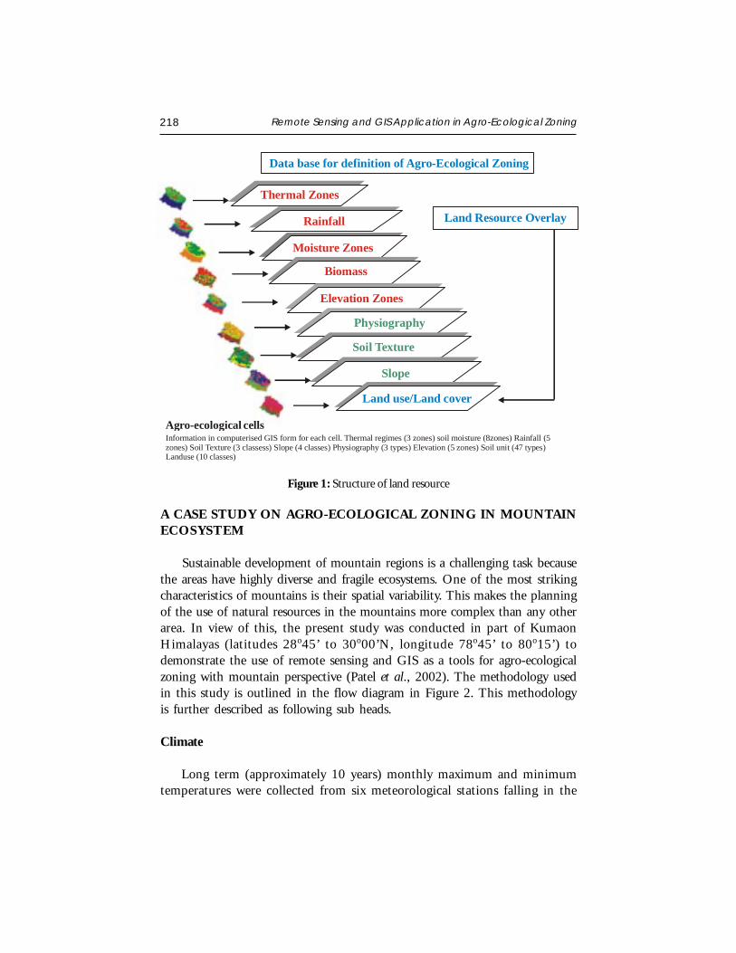
218 Remote Sensing and GIS Application in Agro-Ecological Zoning
A CASE STUDY ON AGRO-ECOLOGICAL ZONING IN MOUNTAINECOSYSTEM
Sustainable development of mountain regions is a challenging task becausethe areas have highly diverse and fragile ecosystems. One of the most strikingcharacteristics of mountains is their spatial variability. This makes the planningof the use of natural resources in the mountains more complex than any otherarea. In view of this, the present study was conducted in part of KumaonHimalayas (latitudes 28o45’ to 30o00’N, longitude 78o45’ to 80o15’) todemonstrate the use of remote sensing and GIS as a tools for agro-ecologicalzoning with mountain perspective (Patel et al., 2002). The methodology usedin this study is outlined in the flow diagram in Figure 2. This methodologyis further described as following sub heads.
Climate
Long term (approximately 10 years) monthly maximum and minimumtemperatures were collected from six meteorological stations falling in the
Figure 1: Structure of land resource
Data base for definition of Agro-Ecological Zoning
Land Resource Overlay
Thermal Zones
Rainfall
Moisture Zones
Agro-ecological cellsInformation in computerised GIS form for each cell. Thermal regimes (3 zones) soil moisture (8zones) Rainfall (5 zones) Soil Texture (3 classess) Slope (4 classes) Physiography (3 types) Elevation (5 zones) Soil unit (47 types) Landuse (10 classes)
Physiography
Elevation Zones
Biomass
Slope
Soil Texture
Land use/Land cover
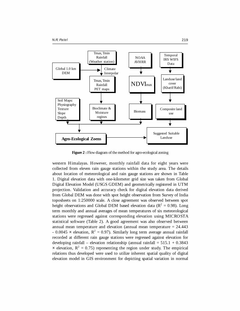
N.R. Patel 219
western Himalayas. However, monthly rainfall data for eight years werecollected from eleven rain gauge stations within the study area. The detailsabout location of meteorological and rain gauge stations are shown in Table1. Digital elevation data with one-kilometer grid size was taken from GlobalDigital Elevation Model (USGS GDEM) and geometrically registered in UTMprojection. Validation and accuracy check for digital elevation data derivedfrom Global DEM was done with spot height observation from Survey of Indiatoposheets on 1:250000 scale. A close agreement was observed between spotheight observations and Global DEM based elevation data (R2 = 0.98). Longterm monthly and annual averages of mean temperatures of six meteorologicalstations were regressed against corresponding elevation using MICROSTAstatistical software (Table 2). A good agreement was also observed betweenannual mean temperature and elevation (annual mean temperature = 24.443- 0.0045 × elevation, R2 = 0.97). Similarly long term average annual rainfallrecorded at different rain gauge stations were regressed against elevation fordeveloping rainfall – elevation relationship (annual rainfall = 515.1 + 0.3843× elevation, R2 = 0.75) representing the region under study. The empiricalrelations thus developed were used to utilize inherent spatial quality of digitalelevation model in GIS environment for depicting spatial variation in normal
Figure 2 : Flow diagram of the method for agro-ecological zoning
Soil Maps:PhysiographyTextureSlopeDepth
Bioclimate &Moistureregines
BiomassComposite land
use
Landuse/landcover
(Kharif/Rabi)
TemporalIRS WIFS
Data
NOAAAVHRR
NDVImaxTmax, Tmin
RainfallPET maps
Suggested SuitableLanduse
Global 1.0 kmDEM
ClimateInterpolar
Tmax, TminRainfall
(Weather station)
Agro-Ecological Zoens
220 Remote Sensing and GIS Application in Agro-Ecological Zoning
monthly and annual mean temperatures as well as annual rainfall conditionover Kumaon region. These monthly spatial distribution of mean temperatureswere used for computation of spatial potential evapotranspiration (PET) basedon Thornthwaite (1948) as:
PET = 1.6 [ (10 Tijk/Ijk)ajk ]
where,
Dec
Ijk = ∑ (Tijk/5)1.514
i =Jan
T = Mean air temperature (°C)
i = Month of a year (i = Jan, Feb, ……Dec)
j = Pixel value of i th row
k = Pixel value of j th column
ajk =67.5*10-8(Ijk)3-7.71*10-5*(Ijk)
2+0.01792( Ijk)+0.4923
These monthly potential evapotranspiration were summed over twelvemonths in a year to obtain spatial distribution of annual PET for use incomputation of moisture index (MI). The moisture index with positive andnegative values indicates moist or dry climate and seasonal variation of effectivemoisture. The revised moisture index of Thornwaite and Mather (1955)method based on annual rainfall and potential evapotranspiration wascalculated as,
MI =[( P – PET)/PET] * 100
where,
MI = Moisture Index
P = Rainfall (mm)
PET = Potential Evapotranspiration (mm)
This information on moisture index is vital to congenial biotic environmentand has been used to classify the climatic types. To arrive at homogeneouszones, the limit of moisture index of the various climatic types was scaled asshown in Table 3.
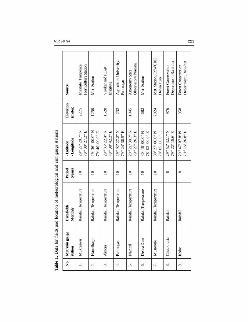
N.R. Patel 221
Tab
le 1
. D
ata
for
field
s an
d lo
cati
on o
f m
eteo
rolo
gica
l an
d ra
in g
auge
sta
tion
s
No.
Met
/rai
n ga
uge
Dat
a fie
lds
Peri
od- L
atitu
deEl
evat
ion
Sour
cest
atio
nM
onth
ly(y
ears
)- L
ongi
tude
(met
er)
1.M
ukte
swar
Rai
nfal
l, Te
mpe
ratu
re10
29 o 2
7’ 2
8.7”
N22
75In
stitu
te T
empe
rate
79 o 3
9’ 2
7.2”
EH
ortic
ultu
re S
tatio
n
2.H
awal
bagh
Rai
nfal
l, Te
mpe
ratu
re10
29o 3
6’ 0
0.0”
N12
50M
et. S
tatio
n79
o 40’
00.
0” E
3.A
lmor
aR
ainf
all,
Tem
pera
ture
1029
o 3
5’ 2
2.4”
N15
28V
ivek
anan
d IC
AR
79 o 3
8’ 4
2.2”
EIn
stitu
te
4.Pa
ntna
gar
Rai
nfal
l, Te
mpe
ratu
re10
29 o 0
2’ 2
7.2”
N23
2A
gric
ultu
re U
nive
rsity
,79
o 2
4’ 3
0.5”
EPa
ntna
gar
5.N
aini
tal
Rai
nfal
l, Te
mpe
ratu
re10
29 o 2
1’ 3
0.7”
N19
45A
stro
nom
y St
ate
79 o 2
7’ 2
6.3”
EO
bser
vato
ry, N
aini
tal
6.D
ehra
Dun
Rai
nfal
l,Tem
pera
ture
1030
o 19’
00.
0” N
682
Met
. Sta
tion
78o 0
2’ 0
0.0”
E
7.M
usso
orie
Rai
nfal
l, Te
mpe
ratu
re10
30o 2
7’ 0
0.0”
N20
24M
et. S
tatio
n, C
SWC
RII
78o 0
5’ 0
0.0”
ED
ehra
Dun
8.C
hauk
hutia
Rai
nfal
l8
29 o 5
2’ 3
2.1”
N97
6Fo
rest
Con
serv
atio
n79
o 2
2’ 1
5.6’
ED
epar
tmen
t, R
anik
het
9.K
edar
Rai
nfal
l8
29 o 4
7’ 0
7.8’
N95
8Fo
rest
Con
serv
atio
n79
o 1
5’ 2
6.8”
ED
epar
tmen
t, R
anik
het
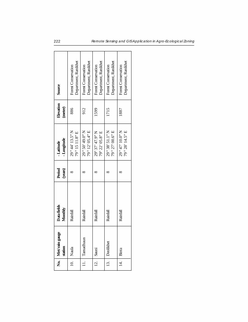
222 Remote Sensing and GIS Application in Agro-Ecological Zoning
10.
Nau
laR
ainf
all
829
o 4
4’ 1
3.5”
N88
6Fo
rest
Con
serv
atio
n79
o 1
5 11
.8”
ED
epar
tmen
t, R
anik
het
11.
Tam
adha
unR
ainf
all
829
o 5
0’ 4
9.0”
N91
2Fo
rest
Con
serv
atio
n79
o 1
2’ 0
5.4”
ED
epar
tmen
t, R
anik
het
12.
Saun
iR
ainf
all
829
o 37’
47.
9” N
1599
Fore
st C
onse
rvat
ion
79o 2
2’ 0
5.8”
ED
epar
tmen
t, R
anik
het
13.
Deo
likhe
tR
ainf
all
829
o 3
8’ 5
1.1”
N17
15Fo
rest
Con
serv
atio
n79
o 2
7’ 0
0.6”
ED
epar
tmen
t, R
anik
het
14.
Bin
taR
ainf
all
829
o 4
7’ 1
0.0”
N18
87Fo
rest
Con
serv
atio
n79
o 2
8’ 1
4.5”
ED
epar
tmen
t, R
anik
het
No.
Met
/rai
n ga
uge
Dat
a fie
lds
Peri
od- L
atitu
deEl
evat
ion
Sour
cest
atio
nM
onth
ly(y
ears
)- L
ongi
tude
(met
er)
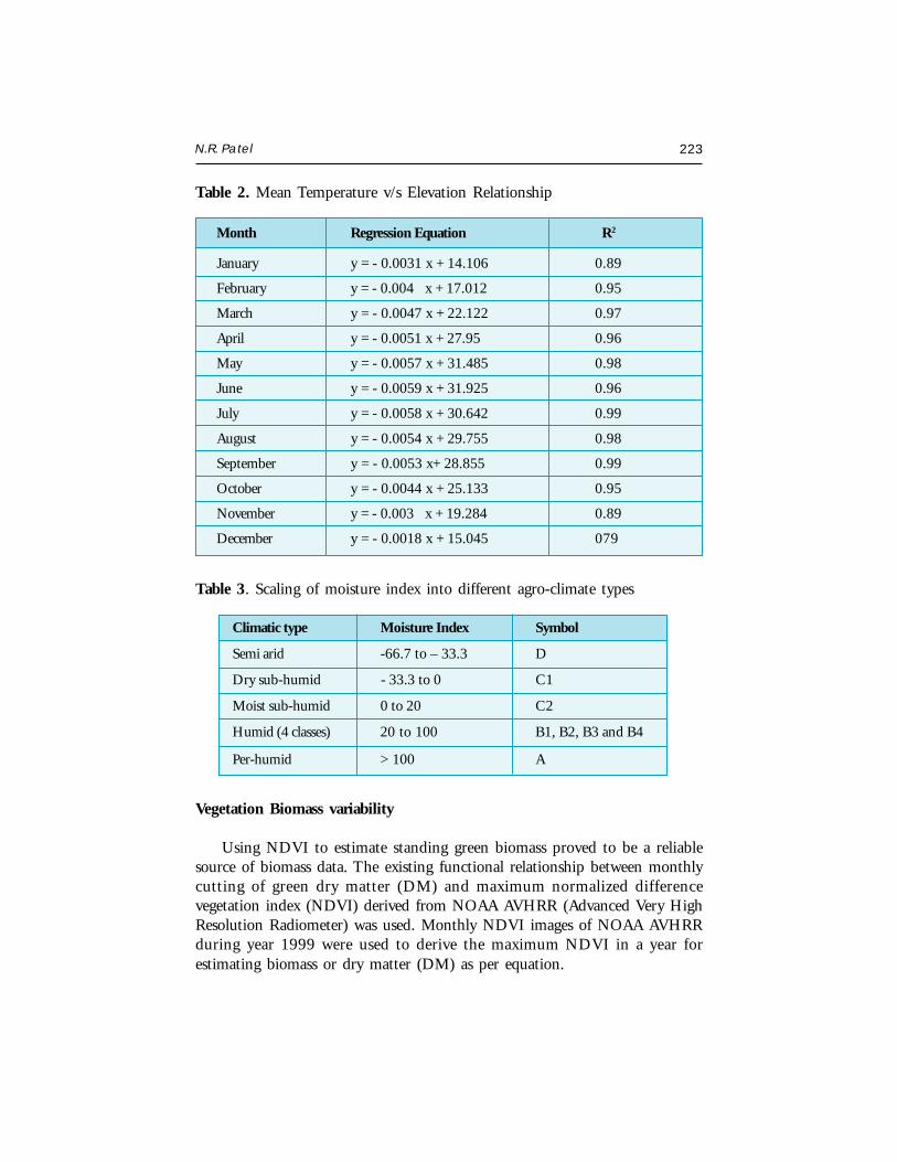
N.R. Patel 223
Table 3. Scaling of moisture index into different agro-climate types
Climatic type Moisture Index Symbol
Semi arid -66.7 to – 33.3 D
Dry sub-humid - 33.3 to 0 C1
Moist sub-humid 0 to 20 C2
Humid (4 classes) 20 to 100 B1, B2, B3 and B4
Per-humid > 100 A
Vegetation Biomass variability
Using NDVI to estimate standing green biomass proved to be a reliablesource of biomass data. The existing functional relationship between monthlycutting of green dry matter (DM) and maximum normalized differencevegetation index (NDVI) derived from NOAA AVHRR (Advanced Very HighResolution Radiometer) was used. Monthly NDVI images of NOAA AVHRRduring year 1999 were used to derive the maximum NDVI in a year forestimating biomass or dry matter (DM) as per equation.
Table 2. Mean Temperature v/s Elevation Relationship
Month Regression Equation R2
January y = - 0.0031 x + 14.106 0.89
February y = - 0.004 x + 17.012 0.95
March y = - 0.0047 x + 22.122 0.97
April y = - 0.0051 x + 27.95 0.96
May y = - 0.0057 x + 31.485 0.98
June y = - 0.0059 x + 31.925 0.96
July y = - 0.0058 x + 30.642 0.99
August y = - 0.0054 x + 29.755 0.98
September y = - 0.0053 x+ 28.855 0.99
October y = - 0.0044 x + 25.133 0.95
November y = - 0.003 x + 19.284 0.89
December y = - 0.0018 x + 15.045 079
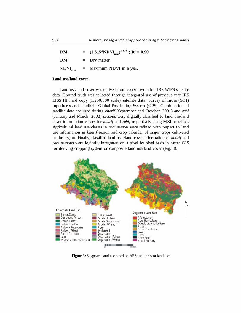
224 Remote Sensing and GIS Application in Agro-Ecological Zoning
DM = (1.615*NDVImax)1.318 ; R2 = 0.90
DM = Dry matter
NDVImax = Maximum NDVI in a year.
Land use/land cover
Land use/land cover was derived from coarse resolution IRS WiFS satellitedata. Ground truth was collected through integrated use of previous year IRSLISS III hard copy (1:250,000 scale) satellite data, Survey of India (SOI)toposheets and handheld Global Positioning System (GPS). Combination ofsatellite data acquired during kharif (September and October, 2001) and rabi(January and March, 2002) seasons were digitally classified to land use/landcover information classes for kharif and rabi, respectively using MXL classifier.Agricultural land use classes in rabi season were refined with respect to landuse information in kharif season and crop calendar of major crops cultivatedin the region. Finally, classified land use /land cover information of kharif andrabi seasons were logically integrated on a pixel by pixel basis in raster GISfor deriving cropping system or composite land use/land cover (Fig. 3).
Figure 3: Suggested land use based on AEZs and present land use
Barren/ScrubDeciduous ForestDense ForestFallow - FallowFallow - SugarcaneFallow - WheatForest PlantationLakeModerately Dense Forest
Open ForestPaddy - FallowPaddy -SugarcanePaddy - WheatRiverSettlementSugarcaneSugarcane - FallowSugarcane - Wheat
AfforestationAgro HorticultureDouble crop agricultureForestForest PlantationLakeRiver SettlementSocial Forestry
Suggested Land UseComposite Land Use
N
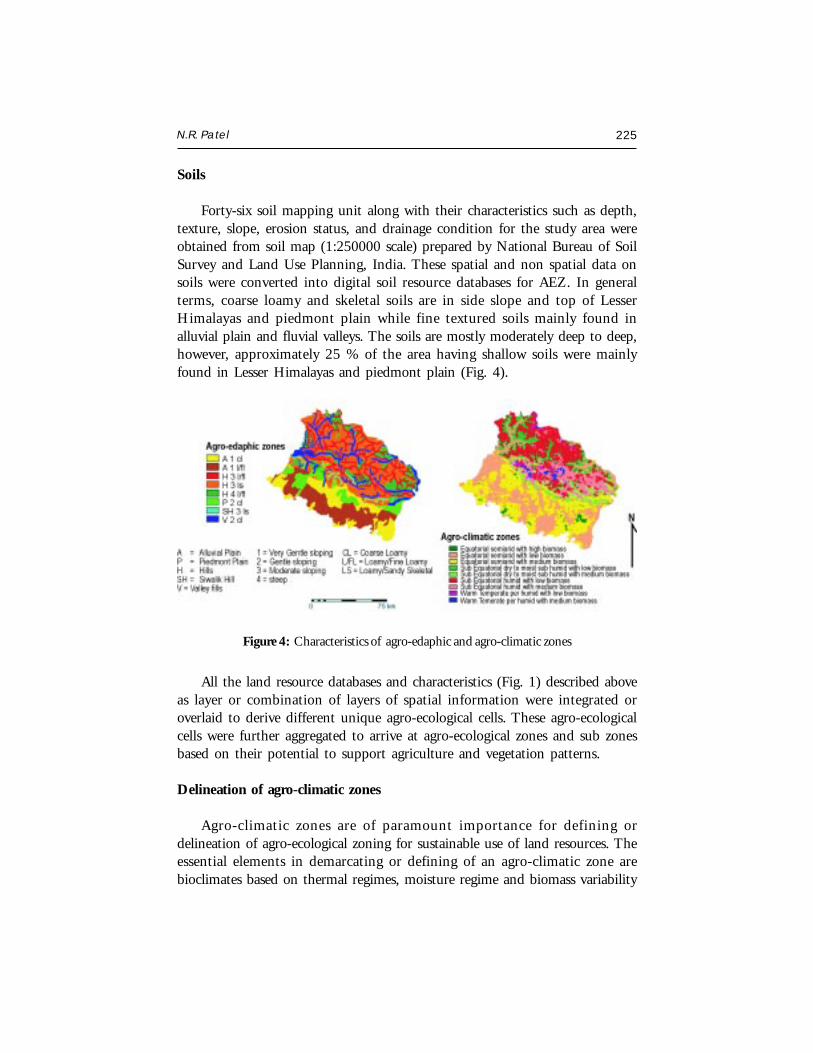
N.R. Patel 225
Soils
Forty-six soil mapping unit along with their characteristics such as depth,texture, slope, erosion status, and drainage condition for the study area wereobtained from soil map (1:250000 scale) prepared by National Bureau of SoilSurvey and Land Use Planning, India. These spatial and non spatial data onsoils were converted into digital soil resource databases for AEZ. In generalterms, coarse loamy and skeletal soils are in side slope and top of LesserHimalayas and piedmont plain while fine textured soils mainly found inalluvial plain and fluvial valleys. The soils are mostly moderately deep to deep,however, approximately 25 % of the area having shallow soils were mainlyfound in Lesser Himalayas and piedmont plain (Fig. 4).
Figure 4: Characteristics of agro-edaphic and agro-climatic zones
All the land resource databases and characteristics (Fig. 1) described aboveas layer or combination of layers of spatial information were integrated oroverlaid to derive different unique agro-ecological cells. These agro-ecologicalcells were further aggregated to arrive at agro-ecological zones and sub zonesbased on their potential to support agriculture and vegetation patterns.
Delineation of agro-climatic zones
Agro-climatic zones are of paramount importance for defining ordelineation of agro-ecological zoning for sustainable use of land resources. Theessential elements in demarcating or defining of an agro-climatic zone arebioclimates based on thermal regimes, moisture regime and biomass variability
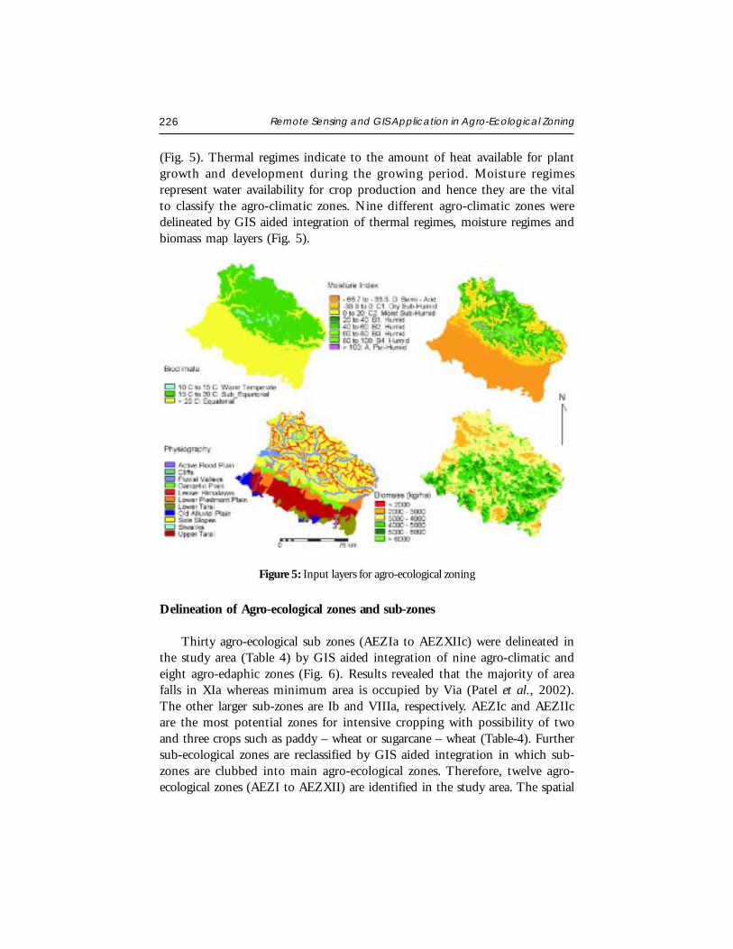
226 Remote Sensing and GIS Application in Agro-Ecological Zoning
(Fig. 5). Thermal regimes indicate to the amount of heat available for plantgrowth and development during the growing period. Moisture regimesrepresent water availability for crop production and hence they are the vitalto classify the agro-climatic zones. Nine different agro-climatic zones weredelineated by GIS aided integration of thermal regimes, moisture regimes andbiomass map layers (Fig. 5).
Figure 5: Input layers for agro-ecological zoning
Delineation of Agro-ecological zones and sub-zones
Thirty agro-ecological sub zones (AEZIa to AEZXIIc) were delineated inthe study area (Table 4) by GIS aided integration of nine agro-climatic andeight agro-edaphic zones (Fig. 6). Results revealed that the majority of areafalls in XIa whereas minimum area is occupied by Via (Patel et al., 2002).The other larger sub-zones are Ib and VIIIa, respectively. AEZIc and AEZIIcare the most potential zones for intensive cropping with possibility of twoand three crops such as paddy – wheat or sugarcane – wheat (Table-4). Furthersub-ecological zones are reclassified by GIS aided integration in which sub-zones are clubbed into main agro-ecological zones. Therefore, twelve agro-ecological zones (AEZI to AEZXII) are identified in the study area. The spatial
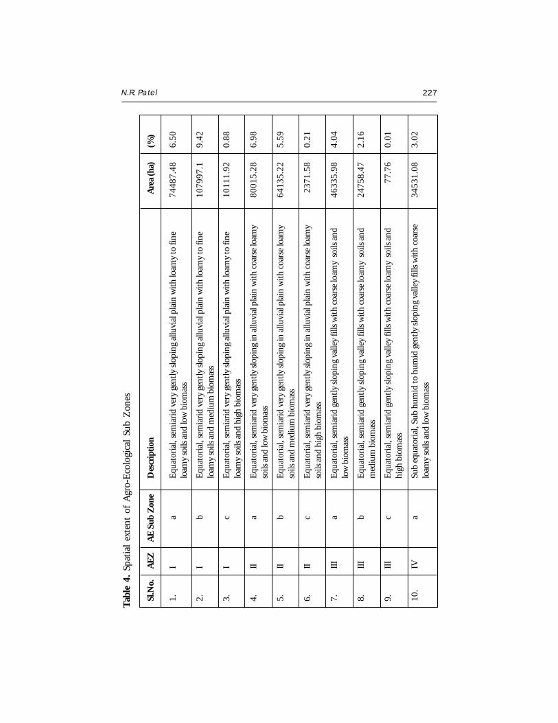
N.R. Patel 227
Tab
le 4
. Sp
atia
l ex
tent
of
Agr
o-E
colo
gica
l Su
b Z
ones
Sl.N
o.A
EZA
E S
ub Z
one
Des
crip
tion
Are
a (h
a)(%
)
1.I
aE
quat
oria
l, se
mia
rid
very
gen
tly sl
opin
g al
luvi
al p
lain
with
loam
y to
fine
7448
7.48
6.50
loam
y so
ils a
nd lo
w b
iom
ass
2.I
bE
quat
oria
l, se
mia
rid
very
gen
tly sl
opin
g al
luvi
al p
lain
with
loam
y to
fine
1079
97.1
9.42
loam
y so
ils a
nd m
ediu
m b
iom
ass
3.I
cE
quat
oria
l, se
mia
rid
very
gen
tly sl
opin
g al
luvi
al p
lain
with
loam
y to
fine
1011
1.92
0.88
loam
y so
ils a
nd h
igh
biom
ass
4.II
aE
quat
oria
l, se
mia
rid
very
gen
tly sl
opin
g in
allu
vial
pla
in w
ith c
oars
e lo
amy
8001
5.28
6.98
soils
and
low
bio
mas
s
5.II
bE
quat
oria
l, se
mia
rid
very
gen
tly sl
opin
g in
allu
vial
pla
in w
ith c
oars
e lo
amy
6413
5.22
5.59
soils
and
med
ium
bio
mas
s
6.II
cE
quat
oria
l, se
mia
rid
very
gen
tly sl
opin
g in
allu
vial
pla
in w
ith c
oars
e lo
amy
2371
.58
0.21
soils
and
hig
h bi
omas
s
7.II
Ia
Equ
ator
ial,
sem
iari
d ge
ntly
slop
ing
valle
y fil
ls w
ith c
oars
e lo
amy
soils
and
4633
5.98
4.04
low
bio
mas
s
8.II
Ib
Equ
ator
ial,
sem
iari
d ge
ntly
slop
ing
valle
y fil
ls w
ith c
oars
e lo
amy
soils
and
2475
8.47
2.16
med
ium
bio
mas
s
9.II
Ic
Equ
ator
ial,
sem
iari
d ge
ntly
slop
ing
valle
y fil
ls w
ith c
oars
e lo
amy
soils
and
77.7
60.
01hi
gh b
iom
ass
10.
IVa
Sub
equa
tori
al, S
ub h
umid
to h
umid
gen
tly sl
opin
g va
lley
fills
with
coa
rse
3453
1.08
3.02
loam
y so
ils a
nd lo
w b
iom
ass
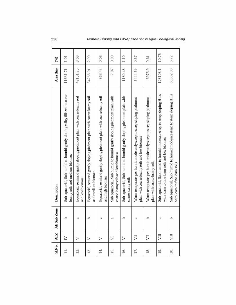
228 Remote Sensing and GIS Application in Agro-Ecological Zoning
11.
IVb
Sub
equa
tori
al, S
ub h
umid
to h
umid
gen
tly sl
opin
g va
lley
fills
with
coa
rse
1163
1.71
1.01
loam
y so
ils a
nd m
ediu
m b
iom
ass
12.
Va
Equ
ator
ial,
sem
iari
d ge
ntly
slop
ing
pied
mon
t pla
in w
ith c
oars
e lo
amy
soil
4215
1.25
3.68
and
low
bio
mas
s
13.
Vb
Equ
ator
ial,
sem
iari
d ge
ntly
slop
ing
pied
mon
t pla
in w
ith c
oars
e lo
amy
soil
3426
6.01
2.99
and
med
ium
bio
mas
s
14.
Vc
Equ
ator
ial,
sem
iari
d ge
ntly
slop
ing
pied
mon
t pla
in w
ith c
oars
e lo
amy
soil
968.
430.
08an
d hi
gh b
iom
ass
15.
VI
aSu
b eq
uato
rial
, Sub
hum
id to
hum
id g
ently
slop
ing
pied
mon
t pla
in w
ith7.
070.
00co
arse
loam
y so
ils a
nd lo
w b
iom
ass
16.
VI
bSu
b eq
uato
rial
, Sub
hum
id to
hum
id g
ently
slop
ing
pied
mon
t pla
in w
ith11
80.4
81.
10co
arse
loam
y so
ils
17.
VII
aW
arm
tem
pera
te, p
er h
umid
mod
erat
ely
stee
p to
stee
p slo
ping
pie
dmon
t54
44.5
90.
57pl
ain
with
coa
rse
loam
y so
ils a
nd lo
w b
iom
ass
18.
VII
bW
arm
tem
pera
te, p
er h
umid
mod
erat
ely
stee
p to
stee
p slo
ping
pie
dmon
t69
76.9
0.61
plai
n w
ith c
oars
e lo
amy
soils
19.
VII
Ia
Sub
equa
tori
al, S
ub h
umid
to h
umid
mod
erat
e st
eep
to st
eep
slopi
ng H
ills
1231
03.1
10.7
5w
ith lo
am to
fine
loam
soils
and
low
bio
mas
s
20.
VII
Ib
Sub
equa
tori
al, S
ub h
umid
to h
umid
mod
erat
e st
eep
to st
eep
slopi
ng H
ills
6566
2.08
5.72
with
loam
to fi
ne lo
am so
ils
Sl.N
o.A
EZA
E S
ub Z
one
Des
crip
tion
Are
a (h
a)(%
)
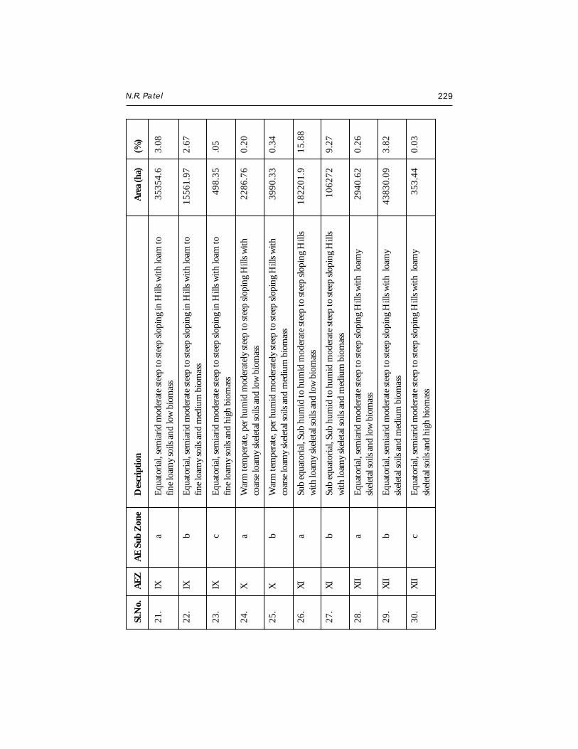
N.R. Patel 229
21.
IXa
Equ
ator
ial,
sem
iari
d m
oder
ate
stee
p to
stee
p slo
ping
in H
ills w
ith lo
am to
3535
4.6
3.08
fine
loam
y so
ils a
nd lo
w b
iom
ass
22.
IXb
Equ
ator
ial,
sem
iari
d m
oder
ate
stee
p to
stee
p slo
ping
in H
ills w
ith lo
am to
1556
1.97
2.67
fine
loam
y so
ils a
nd m
ediu
m b
iom
ass
23.
IXc
Equ
ator
ial,
sem
iari
d m
oder
ate
stee
p to
stee
p slo
ping
in H
ills w
ith lo
am to
498.
35.0
5fin
e lo
amy
soils
and
hig
h bi
omas
s
24.
Xa
War
m te
mpe
rate
, per
hum
id m
oder
atel
y st
eep
to st
eep
slopi
ng H
ills w
ith22
86.7
60.
20co
arse
loam
y sk
elet
al so
ils a
nd lo
w b
iom
ass
25.
Xb
War
m te
mpe
rate
, per
hum
id m
oder
atel
y st
eep
to st
eep
slopi
ng H
ills w
ith39
90.3
30.
34co
arse
loam
y sk
elet
al so
ils a
nd m
ediu
m b
iom
ass
26.
XI
aSu
b eq
uato
rial
, Sub
hum
id to
hum
id m
oder
ate
stee
p to
stee
p slo
ping
Hill
s18
2201
.915
.88
with
loam
y sk
elet
al so
ils a
nd lo
w b
iom
ass
27.
XI
bSu
b eq
uato
rial
, Sub
hum
id to
hum
id m
oder
ate
stee
p to
stee
p slo
ping
Hill
s10
6272
9.27
with
loam
y sk
elet
al so
ils a
nd m
ediu
m b
iom
ass
28.
XII
aE
quat
oria
l, se
mia
rid
mod
erat
e st
eep
to st
eep
slopi
ng H
ills w
ith l
oam
y29
40.6
20.
26sk
elet
al so
ils a
nd lo
w b
iom
ass
29.
XII
bE
quat
oria
l, se
mia
rid
mod
erat
e st
eep
to st
eep
slopi
ng H
ills w
ith l
oam
y43
830.
093.
82sk
elet
al so
ils a
nd m
ediu
m b
iom
ass
30.
XII
cE
quat
oria
l, se
mia
rid
mod
erat
e st
eep
to st
eep
slopi
ng H
ills w
ith l
oam
y35
3.44
0.03
skel
etal
soils
and
hig
h bi
omas
s
Sl.N
o.A
EZA
E S
ub Z
one
Des
crip
tion
Are
a (h
a)(%
)
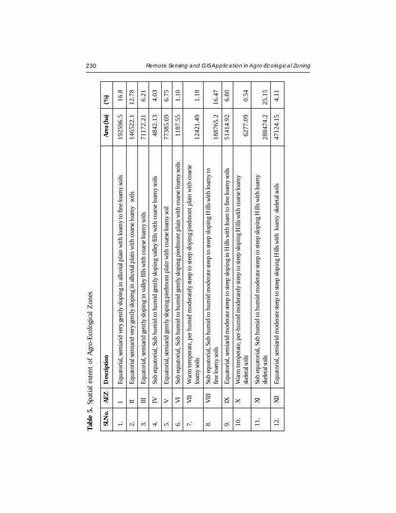
230 Remote Sensing and GIS Application in Agro-Ecological Zoning
Tab
le 5
. Sp
atia
l ex
tent
of
Agr
o-E
colo
gica
l Z
ones
Sl.N
o.A
EZD
escr
iptio
nA
rea
(ha)
(%)
1.I
Equ
ator
ial,
sem
iari
d ve
ry g
ently
slop
ing
in a
lluvi
al p
lain
with
loam
y to
fine
loam
y so
ils19
2596
.516
.8
2.II
Equ
ator
ial s
emia
rid
very
gen
tly sl
opin
g in
allu
vial
pla
in w
ith c
oars
e lo
amy
soi
ls14
6522
.112
.78
3.II
IE
quat
oria
l, se
mia
rid
gent
ly sl
opin
g in
val
ley
fills
with
coa
rse
loam
y so
ils71
172.
216.
21
4.IV
Sub
equa
tori
al, S
ub h
umid
to h
umid
gen
tly sl
opin
g va
lley
fills
with
coa
rse
loam
y so
ils48
42.1
34.
03
5.V
Equ
ator
ial,
sem
iari
d ge
ntly
slop
ing
pied
mon
t pla
in w
ith c
oars
e lo
amy
soil
7738
5.69
6.75
6.V
ISu
b eq
uato
rial
, Sub
hum
id to
hum
id g
ently
slop
ing
pied
mon
t pla
in w
ith c
oars
e lo
amy
soils
1187
.55
1.10
7.V
IIW
arm
tem
pera
te, p
er h
umid
mod
erat
ely
stee
p to
stee
p slo
ping
pie
dmon
t pla
in w
ith c
oars
elo
amy
soils
1242
1.49
1.18
8.V
III
Sub
equa
tori
al, S
ub h
umid
to h
umid
mod
erat
e st
eep
to st
eep
slopi
ng H
ills w
ith lo
amy
tofin
e lo
amy
soils
1887
65.2
16.4
7
9.IX
Equ
ator
ial,
sem
iari
d m
oder
ate
stee
p to
stee
p slo
ping
in H
ills w
ith lo
am to
fine
loam
y so
ils51
414.
926.
80
10.
XW
arm
tem
pera
te, p
er-h
umid
mod
erat
ely
stee
p to
stee
p slo
ping
Hill
s with
coa
rse
loam
ysk
elet
al so
ils62
77.0
90.
54
11.
XI
Sub
equa
tori
al, S
ub h
umid
to h
umid
mod
erat
e st
eep
to st
eep
slopi
ng H
ills w
ith lo
amy
skel
etal
soils
2884
74.2
25.1
5
12.
XII
Equ
ator
ial,
sem
iari
d m
oder
ate
stee
p to
stee
p slo
ping
Hill
s with
loa
my
skel
etal
soils
4712
4.15
4.11
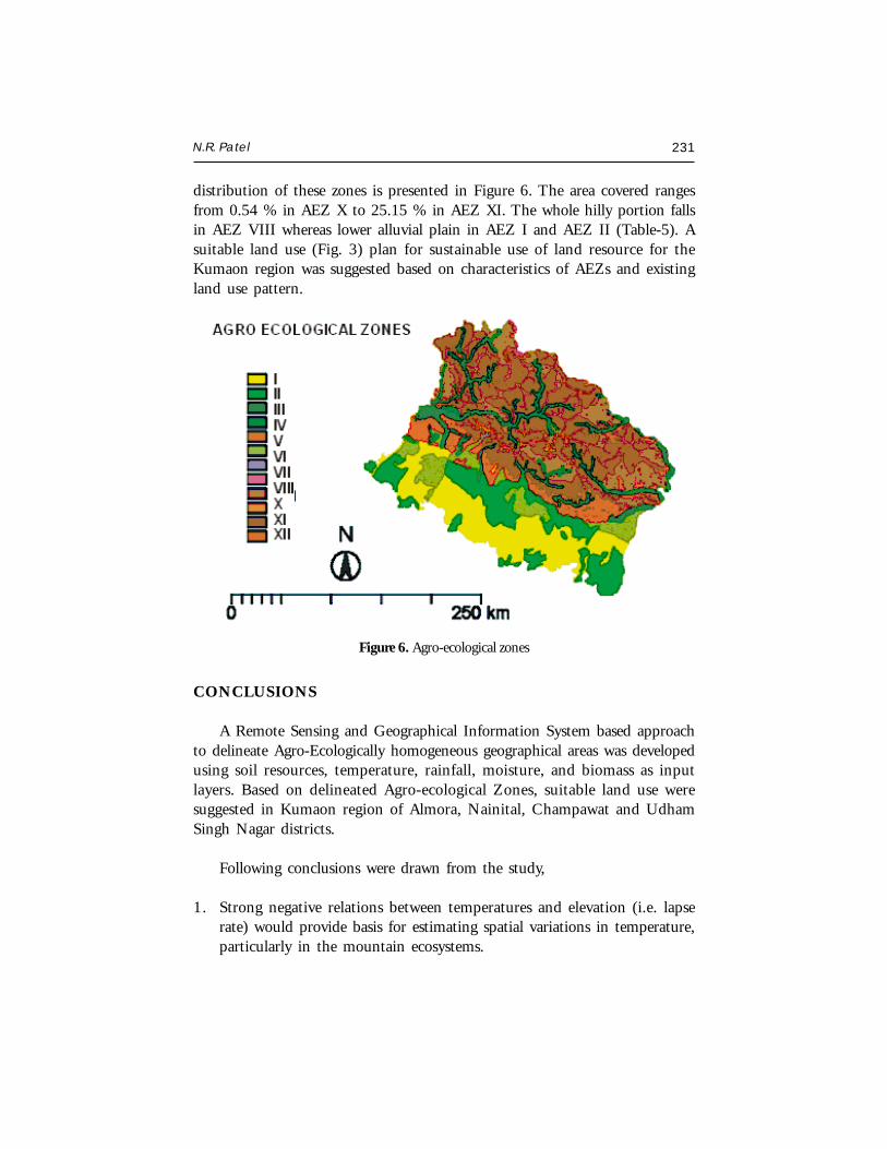
N.R. Patel 231
distribution of these zones is presented in Figure 6. The area covered rangesfrom 0.54 % in AEZ X to 25.15 % in AEZ XI. The whole hilly portion fallsin AEZ VIII whereas lower alluvial plain in AEZ I and AEZ II (Table-5). Asuitable land use (Fig. 3) plan for sustainable use of land resource for theKumaon region was suggested based on characteristics of AEZs and existingland use pattern.
Figure 6. Agro-ecological zones
CONCLUSIONS
A Remote Sensing and Geographical Information System based approachto delineate Agro-Ecologically homogeneous geographical areas was developedusing soil resources, temperature, rainfall, moisture, and biomass as inputlayers. Based on delineated Agro-ecological Zones, suitable land use weresuggested in Kumaon region of Almora, Nainital, Champawat and UdhamSingh Nagar districts.
Following conclusions were drawn from the study,
1. Strong negative relations between temperatures and elevation (i.e. lapserate) would provide basis for estimating spatial variations in temperature,particularly in the mountain ecosystems.
232 Remote Sensing and GIS Application in Agro-Ecological Zoning
2. Spatial distribution of PET and Moisture index would help in definingmicro-Environment more accurately in the mountains environment.
3. Integration of bio-climate, moisture regimes and regional vegetationbiomass in GIS environment could provide a more dynamic way ofcharacterizing homogeneous agro-climatic zones for identifying biophysicaland climate characteristics to agricultural productivity.
REFERENCES
Carter, D.B. 1954. Climates of Africa and according to Thornthwaite (1948) Classification.John Hopkins University Publication (in) Climatology, 7(14).
FAO, 1976. A framework for land evaluation. Food and Agricultural Organisation, SoilsBulletin 32, Rome, Italy.
FAO, 1996. Guidelines: Agro-ecological zoning. Food and Agricultural Organisation, SoilsBulletin, Rome, Italy.
Krishnan, A. 1988. Delineation of soil climatic zones of India and its practical applicationsin Agriculture. Fertilizer News, 33 (4).
Mavi, H.S. 1984. Introduction to Agrometeorology, IInd edition. Raju Primlani for Oxford& IBH Publishers Co. Pvt. Ltd.
Murthy, R.S. and Pandey, S. 1978. Delineation of agro-ecological regions of India. Paperpresented in Commission V, 11th Congress of ISSS, Edmonton, Canada, June 19-27.
Pariyar, M.P. and Singh, G. 1994. GIS based model for agro-ecological zoning: a case studyof Chitwan district, Nepal. Proc. 15th Asian Conference Rem. Sens., Bangalore, India.Vol. 1 : A4-1 to A4-6.
Pratap, T., Pradhan, P., Lotta, P.K., Mya, S., Karim and Nakarmi, G. 1992. GeographicInformation Systems and Technology application in Agro-ecological zonation ofmountain agriculture. Eds. N.S. Jodha, M. Banskota and Tej Pratap, Oxford & IBHPublishing Co. Pvt. Ltd., New Delhi.
Patel, N.R., Mandal, U.K. and Pande, L.M. 2000. Agro-ecological zoning system. A RemoteSensing and GIS Perspective. Journal of Agrometeorology, 2 (1) : 1-13.
Patel, N.R., Endang, P., Suresh Kumar and Pande, L.M. 2002. Agro-ecological zoning usingremote sensing and GIS – A case study in part of Kumaon region. In: Sustainableagriculture development, Proce. of 2nd International Conference on SustainableAgriculture, Water Resources Development and Earth Care Policies, 18-20 December,2002, New Delhi (In Press).
N.R. Patel 233
Sehgal, J.L., Vernemmen, C. and Tavernier, R. 1987. Agro-climatic Environments andMoisture Regimes in NW India - Their Applications in Soils and Crop Growth. ResearchBull. NBSS Publ. 17, Nagpur, India, NBSS & LUP.
Sehgal, J.L., Mandal, D.K., Mandal, C. and Vadivelu, S. 1992. Agro-ecological Region ofIndia. NBSS & LUP (ICAR) Publication 24, Nagpur.
Subramanian, A.R. 1983. Agro-ecological Zones of India. Arch. Met. Geoph. Biocl. Ser. B32;329-333.
Thornthwaite, C.E. and Mathew, J.R. 1955. The Water Balance. Publications in Climatology,Vol.8, No.1. Drexel Institute of Technology, Laboratory of Climatology, Centerton, N.J.pp. 104.
Thornthwaite, C.W. 1948. An Approach towards a rational classification of climate.Geographical Review, 38: 55-94.
Troll, C. 1965. Seasonal Climates of the earth. World maps of Climatology. Eds. E. Rodenwaltand H. Jusatz. Berlin : Springer – Verlag, pp. 28.
Venkateshwarlu, J., Ramakrishna, Y.S. and Rao, A.S. 1996. Agro-climatic zones of India.Annals of Arid Zone, 35 (1); 1-8.
Verma and Pratap, 1989. Agro climatic zones. Profiles and Issues. Agro-climatic RegionalPlanning UNIT (ARPU) Working paper, Ahmedabad: Sardar Patel Inst. of Econ. andSoc. Res. 1989.
CROP GROWTH MODELING AND ITSAPPLICATIONS IN AGRICULTURALMETEOROLOGY
V. Radha Krishna MurthyDepartment of Agronomy, College of AgricultureANGR Agricultural University, Rajendranagar, Hyderabad
Abstract: This paper discusses various crop growth modeling approaches viz.Statistical, Mechanistic, Deterministic, Stochastic, Dynamic, Static and Simulationetc. Role of climate change in crop modeling and applications of crop growthmodels in agricultural meteorology are also discussed. A few successfully usedcrop growth models in agrometeorology are discussed in detail.
INTRODUCTION
Crop is defined as an “Aggregation of individual plant species grown in aunit area for economic purpose”.
Growth is defined as an “Irreversible increase in size and volume and isthe consequence of differentiation and distribution occurring in the plant”.
Simulation is defined as “Reproducing the essence of a system withoutreproducing the system itself ”. In simulation the essential characteristics ofthe system are reproduced in a model, which is then studied in an abbreviatedtime scale.
A model is a schematic representation of the conception of a system or anact of mimicry or a set of equations, which represents the behaviour of a system.Also, a model is “A representation of an object, system or idea in some formother than that of the entity itself ”. Its purpose is usually to aid in explaining,understanding or improving performance of a system. A model is, by definition
Satellite Remote Sensing and GIS Applications in Agricultural Meteorologypp. 235-261
236 Crop Growth Modeling and its Applications in Agricultural Meteorology
“A simplified version of a part of reality, not a one to one copy”. Thissimplification makes models useful because it offers a comprehensivedescription of a problem situation. However, the simplification is, at the sametime, the greatest drawback of the process. It is a difficult task to produce acomprehensible, operational representation of a part of reality, which graspsthe essential elements and mechanisms of that real world system and evenmore demanding, when the complex systems encountered in environmentalmanagement (Murthy, 2002).
The Earth’s land resources are finite, whereas the number of people thatthe land must support continues to grow rapidly. This creates a major problemfor agriculture. The production (productivity) must be increased to meetrapidly growing demands while natural resources must be protected. Newagricultural research is needed to supply information to farmers, policy makersand other decision makers on how to accomplish sustainable agriculture overthe wide variations in climate around the world. In this direction explanationand prediction of growth of managed and natural ecosystems in response toclimate and soil-related factors are increasingly important as objectives ofscience. Quantitative prediction of complex systems, however, depends onintegrating information through levels of organization, and the principalapproach for that is through the construction of statistical and simulationmodels. Simulation of system’s use and balance of carbon, beginning with theinput of carbon from canopy assimilation forms the essential core of mostsimulations that deal with the growth of vegetation.
Systems are webs or cycles of interacting components. Change in onecomponent of a system produces changes in other components because of theinteractions. For example, a change in weather to warm and humid may leadto the more rapid development of a plant disease, a loss in yield of a crop,and consequent financial adversity for individual farmers and so for the peopleof a region. Most natural systems are complex. Many do not have boundaries.The bio-system is comprised of a complex interaction among the soil, theatmosphere, and the plants that live in it. A chance alteration of one elementmay yield both desirable and undesirable consequences. Minimizing theundesirable, while reaching the desired end result is the principle aim of theagrometerologist. In any engineering work related to agricultural meteorologythe use of mathematical modeling is essential. Of the different modelingtechniques, mathematical modeling enables one to predict the behaviour ofdesign while keeping the expense at a minimum. Agricultural systems arebasically modified ecosystems. Managing these systems is very difficult. These
V. Radha Krishna Murthy 237
systems are influenced by the weather both in length and breadth. So, thesehave to be managed through systems models which are possible only throughclassical engineering expertise.
TYPES OF MODELS
Depending upon the purpose for which it is designed the models areclassified into different groups or types. Of them a few are :
a. Statistical models: These models express the relationship between yieldor yield components and weather parameters. In these models relationshipsare measured in a system using statistical techniques (Table 1).
Example: Step down regressions, correlation, etc.
b. Mechanistic models: These models explain not only the relationshipbetween weather parameters and yield, but also the mechanism of thesemodels (explains the relationship of influencing dependent variables). Thesemodels are based on physical selection.
c. Deterministic models: These models estimate the exact value of the yieldor dependent variable. These models also have defined coefficients.
d. Stochastic models: A probability element is attached to each output. Foreach set of inputs different outputs are given alongwith probabilities. Thesemodels define yield or state of dependent variable at a given rate.
e. Dynamic models: Time is included as a variable. Both dependent andindependent variables are having values which remain constant over a givenperiod of time.
f. Static: Time is not included as a variables. Dependent and independentvariables having values remain constant over a given period of time.
g. Simulation models: Computer models, in general, are a mathematicalrepresentation of a real world system. One of the main goals of cropsimulation models is to estimate agricultural production as a function ofweather and soil conditions as well as crop management. These modelsuse one or more sets of differential equations, and calculate both rate andstate variables over time, normally from planting until harvest maturityor final harvest.
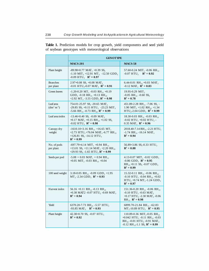
238 Crop Growth Modeling and its Applications in Agricultural Meteorology
Table 1. Prediction models for crop growth, yield components and seed yieldof soybean genotypes with meteorological observations
GENOTYPE
MACS-201 MACS-58
Plant height -89.98+0.77 MAT1 +0.39 SS2 57.60-0.24 MIT1 -0.06 RH12
-1.10 MIT3 +12.91 MT3 -12.50 GDD3 -0.07 HTU3 R2 = 0.92
-0.09 HTU3 R2 = 0.97
Branches 2.97+0.08 SS1 +0.08 MAT2 6.44-0.01 RH21 +0.03 MAT2
per plant -0.01 HTU2-0.07 MAT3 R2 = 0.91 -0.12 MAT3 R
2 = 0.83
Green leaves -1.20-0.20 MT1 -0.03 RH11 +0.19 19.95-0.29 MIT2
GDD2 -0.18 RH13 +0.13 RH23 -0.05 RH12 -0.60 SS3
+2.92 MT3 -3.55 GDD3 R2 = 0.98 R2 = 0.78
Leaf area 754.01-25.97 SS1 -20.65 MAT2 451.89-2.28 RH11 -7.06 SS1 -(dm2 m-2) -29.85 SS2 +0.15 HTU2 -23.23 MIT3 1.90 MIT2 +1.02 RH22 +1.34
-5.66 RH13 -0.73 RH23 R2 = 0.99 HTU2-2.04 GDD3 R
2 = 0.99
Leaf area index -13.46+0.40 SS1 -0.09 MAT2 18.30-0.03 RH11 -0.03 RH21
+0.17 MAT3 +0.15 RH23 +1.02 SS3 -0.02 HTU1 +0.02 HTU2 --0.02 HTU3 R
2 = 0.98 0.35 MAT3 R2 = 0.96
Canopy dry -1610.10+3.16 RH11 +16.65 MT1 2018.40-7.14 RH11 -2.21 HTU1
weight +2.73 HTU2 +76.04 MAT3 -6.77 RH13 -1.74 RH12 -16.14 MAT3
+126.81 SS3 -14.12 HTU3 R2 = 0.94R2 = 0.99
No. of pods -697.79+4.14 MIT1 +0.94 RH11 56.89+3.86 SS1-0.33 HTU3
per plant +13.01 SS1 +11.14 MAT3 +2.20 RH23 R2 = 0.88+29.93 SS3 -1.65 HTU3 R
2 = 0.99
Seeds per pod -5.08 + 0.03 MAT1 + 0.94 RH11 4.13-0.07 MIT1 -0.02 GDD1
+0.05 MIT2 -0.03 RH13 +0.04 -0.86 GDD3 R2 = 0.95
RH23 +0.11 SS3 -0.07 GDD3
R2 = 0.99
100 seed weight 3.18-0.05 RH11 -0.09 GDD2 +1.95 15.32-0.11 RH11 -0.06 RH21
MT3 -2.34 GDD3 R2 = 0.93 -0.10 HTU1 -0.04 RH22 +0.02
HTU2 +0.74 MT3 -1.24 GDD3
R2 = 0.97
Harvest index 56.16 +0.11 RH11 -0.13 RH21 151.36-0.20 RH11 -0.06 RH21
+0.38 MAT2 -0.07 HTU2 -0.69 MAT3 -0.10 HTU1 -0.63 MAT2
R2 = 0.94 +0.17 HTU2 -2.30 MAT3 -0.06RH13 R
2 = 0.98
Yield 6370.20-7.73 RH21 -5.57 HTU2 6899.70-21.84 RH11 -62.83-93.85 MAT3 R
2 = 0.93 MT1-10.89 HTU3 R2 = 0.95
Plant height 42.38+0.70 SS1 -0.07 HTU3 110.89-0.36 MIT1-0.05 RH21
R2 = 0.92 +0.042 HTU1 -0.11 RH12 -0.03RH22 -0.01 HTU2 -0.91 MAT3
-0.12 RH13-1.1 SS3 R2 = 0.99
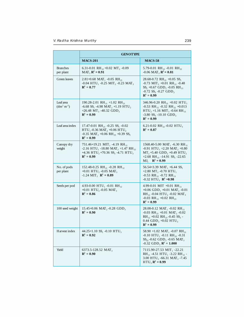
V. Radha Krishna Murthy 239
Branches 6.31-0.01 RH12 +0.02 MT2 -0.09 5.79-0.01 RH12 -0.01 RH22
per plant MAT3 R2 = 0.91 -0.06 MAT3 R
2 = 0.81
Green leaves 2.81+0.68 MAT1 -0.05 RH21 28.68-0.72 RH21 +0.05 SS1
-0.04 HTU1 -0.25 MIT2 -0.23 MAT3 -0.73 MIT2 +0.01 RH12 -0.48R2 = 0.77 SS2 +0.67 GDD2 -0.05 RH13
-0.72 SS3 -0.27 GDD3
R2 = 0.99
Leaf area 190.28-2.01 RH11 +1.02 RH21 346.96-0.20 RH21 +0.02 HTU1
(dm2 m-2) -6.68 SS1 -4.98 MAT2 +1.19 HTU2 -0.53 RH12 -0.32 RH22 +0.013+26.48 MT3 -40.32 GDD3 HTU2 +1.16 MIT3 -0.64 RH13
R2 = 0.99 -3.80 SS3 -10.10 GDD3
R2 = 0.99
Leaf area index 17.47-0.01 RH21 -0.25 SS1 -0.02 6.21-0.02 RH22 -0.02 HTU3
HTU1 -0.36 MAT2 +0.06 HTU2 R2 = 0.87-0.35 MAT3 +0.06 RH23 +0.39 SS3
R2 = 0.99
Canopy dry 751.46+19.21 MIT1 -4.19 RH11 1568.40-5.00 MAT1 -6.30 RH11
weight -2.16 HTU1 -18.80 MAT2 +1.47 RH12 -0.91 HTU1 +2.20 MAT2 +0.80+4.36 HTU2 +70.36 SS3 -4.71 HTU3 MT2 +5.40 GDD2 +0.49 HTU2
R2 = 0.99 +2.68 RH13 -14.91 SS3 -22.65MJ1 R
2 = 0.99
No. of pods 152.48-0.25 RH21 -0.28 RH12 56.54+3.39 MAT1 +6.44 SS1
per plant +0.01 HTU2 -0.05 MAT3 +2.80 MT2 -0.70 HTU1
-1.24 MIT2 R2 = 0.89 -0.53 RH12 -0.72 RH13
-0.32 HTU3 R2 =0.98
Seeds per pod 4.93-0.00 HTU1 -0.01 RH12 4.99-0.01 MIT +0.01 RH11
+0.01 HTU2 -0.05 MAT3 +0.06 GDD1 +0.01 MAT2 -0.01R2 = 0.86 RH12 -0.04 HTU2 -0.02 MAT3
-0.03 RH13 +0.02 RH23
R2 = 0.99
100 seed weight 15.45+0.06 MAT2 -0.28 GDD3 28.08-0.12 MAT1 -0.02 RH11
R2 = 0.90 -0.03 RH21 +0.01 MAT2 -0.02RH12 +0.02 RH23 -0.45 SS3 -0.44 GDD3 +0.02 HTU3
R2 = 0.99
Harvest index 44.25+1.10 SS1 -0.10 HTU3 58.90 +1.02 MAT1 -0.07 RH21
R2 = 0.92 -0.10 HTU1 -0.11 RH22 -0.31SS22 -0.62 GDD2 -0.65 MAT3
-0.32 GDD3 R2 = 1.000
Yield 6373.5-128.52 MAT3 7115.90-27.53 MIT1 -22.21R2 = 0.90 RH11 -4.51 HTU1 -3.22 RH12 -
3.00 HTU2 -66.31 MAT3 -7.45HTU3 R
2 = 0.99
GENOTYPE
MACS-201 MACS-58
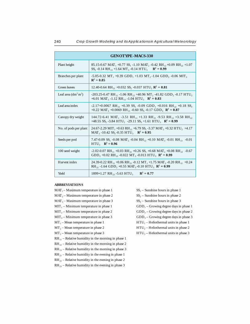
240 Crop Growth Modeling and its Applications in Agricultural Meteorology
GENOTYPE -MACS-330
Plant height 85.15-0.67 MAT1 +0.77 SS1 -1.10 MAT2 -0.42 RH12 +0.09 RH22 +1.07SS2 -0.14 RH13 +1.64 MT3 -0.14 HTU3 R
2 = 0.99
Branches per plant -5.05-0.32 MT1 +0.39 GDD1 +1.03 MT2 -1.04 GDD2 -0.06 MIT3
R2 = 0.85
Green leaves 12.40-0.64 RH21 +0.032 SS2 -0.037 HTU2 R2 = 0.81
Leaf area (dm2 m2) -203.25-0.47 RH11 -1.06 RH12 +40.96 MT2 -41.82 GDD2 -0.17 HTU2
+6.01 MAT3 -1.12 RH13 -1.04 HTU3 R2 = 0.83
Leaf area index -2.17+0.0067 RH21 +0.39 SS1 -0.09 GDD1 +0.016 RH22 +0.18 SS2
+0.22 MAT3 +0.0069 RH13 -0.60 SS3 -0.17 GDD3 R2 = 0.87
Canopy dry weight 144.72-6.41 MAT1 -3.51 RH11 +1.33 RH21 -9.53 RH12 +3.58 RH22
+48.55 SS2 -3.84 HTU2 -29.11 SS3 +1.61 HTU3 R2 = 0.99
No. of pods per plant 24.67-2.29 MIT1 +0.63 RH11 +6.79 SS1 -3.37 MAT2 +0.32 HTU2 +4.17MAT3 -10.42 SS3 -0.35 HTU3 R
2 = 0.95
Seeds per pod 7.47-0.09 SS1 -0.08 MAT2 -0.04 RH12 +0.10 MAT3 -0.01 RH13 -0.01HTU3 R
2 = 0.96
100 seed weight -2.02-0.07 RH11 +0.03 RH21 +0.26 SS1 +0.68 MAT2 +0.08 RH22 -0.67GDD2 +0.02 RH13 -0.022 MT3 -0.013 HTU3 R
2 = 0.99
Harvest index 24.39-0.22 RH11 +0.06 RH21 -0.12 MT1 +1.75 MAT2 -0.20 RH12 +0.24RH22 -1.64 GDD2 +0.55 MAT3 -0.10 HTU3 R
2 = 0.99
Yield 1899+1.27 RH23 -5.63 HTU3 R2 = 0.77
ABBREVIATIONS
MAT1 – Maximum temperature in phase 1 SS1 – Sunshine hours in phase 1
MAT2 – Maximum temperature in phase 2 SS2 – Sunshine hours in phase 2
MAT3 – Maximum temperature in phase 3 SS3 – Sunshine hours in phase 3
MIT1 – Minimum temperature in phase 1 GDD1 – Growing degree days in phase 1
MIT2 – Minimum temperature in phase 2 GDD2 – Growing degree days in phase 2
MIT3 – Minimum temperature in phase 3 GDD3 – Growing degree days in phase 3
MT1 – Mean temperature in phase 1 HTU1 – Heliothermal units in phase 1
MT2 – Mean temperature in phase 2 HTU2 – Heliothermal units in phase 2
MT3 – Mean temperature in phase 3 HTU3 – Heliothermal units in phase 3
RH11 – Relative humidity in the morning in phase 1
RH12 – Relative humidity in the morning in phase 2
RH13 – Relative humidity in the morning in phase 3
RH21 – Relative humidity in the evening in phase 1
RH22 – Relative humidity in the evening in phase 2
RH23 – Relative humidity in the evening in phase 3
V. Radha Krishna Murthy 241
h. Descriptive model: A descriptive model defines the behaviour of a systemin a simple manner. The model reflects little or none of the mechanismsthat are the causes of phenomena. But, consists of one or moremathematical equations. An example of such an equation is the one derivedfrom successively measured weights of a crop. The equation is helpful todetermine quickly the weight of the crop where no observation was made.
i. Explanatory model: This consists of quantitative description of themechanisms and processes that cause the behaviour of the system. To createthis model, a system is analyzed and its processes and mechanisms arequantified separately. The model is built by integrating these descriptionsfor the entire system. It contains descriptions of distinct processes suchas leaf area expansion, tiller production, etc. Crop growth is a consequenceof these processes.
WEATHER DATA FOR MODELING
The national meteorological organizations provide weather data for cropmodeling purposes through observatories across the globe (Sivakumar et al.,2000). In many European countries weather records are available for over 50years. In crop modeling the use of meteorological data has assumed aparamount importance. There is a need for high precision and accuracy ofthe data. The data obtained from surface observatories has proved to beexcellent. It gained the confidence of the people across the globe for decades.These data are being used daily by people from all walks of life. But, theautomated stations are yet to gain popularity in the under developed anddeveloping countries. There is a huge gap between the old time surfaceobservatories and present generation of automated stations with reference tomeasurement of rainfall. The principles involved in the construction andworking of different sensors for measuring rainfall are not commonly followedin automated stations across the globe. As of now, solar radiation, temperatureand precipitation are used as inputs in DSSAT.
Weather as an Input in Models
In crop modeling weather is used as an input. The available data rangesfrom one second to one month at different sites where crop-modeling workin the world is going on. Different curve fitting techniques, interpolation,extrapolation functions etc., are being followed to use weather data in the modeloperation. Agrometeorological variables are especially subject to variations inspace. It is reported that, as of now, anything beyond daily data proved
242 Crop Growth Modeling and its Applications in Agricultural Meteorology
unworthy as they are either over-estimating or under-estimating the yield insimulation. Stochastic weather models can be used as random numbergenerators whose input resembles the weather data to which they have beenfit. These models are convenient and computationally fast, and are useful in anumber of applications where the observed climate record is inadequate withrespect to length, completeness, or spatial coverage. These applications includesimulation of crop growth, development and impacts of climate change. In1995 JW Jones and Thornton described a procedure to link a third-orderMarkov Rainfall model to interpolated monthly mean climate surfaces. Theconstructed surfaces were used to generate daily weather data (rainfall and solarradiation). These are being used for purposes of system characterization andto drive a wide variety of crop and live stock production and ecosystem models.The present generation of crop simulation models particularly DSSAT suit ofmodels have proved their superiority over analytical, statistical, empirical,combination of two or all etc., models so far available. In the earliest cropsimulation models only photosynthesis and carbon balance were simulated.Other processes such as vegetative and reproductive development, plant waterbalance, micronutrients, pest and disease, etc., are not accounted for as thestatistical models use correlative approach and make large area yield predictionand only final yield data are correlated with the regional mean weather variables.This approach has slowly been replaced by the present simulation models bythese DSSAT models. When many inputs are added in future the modelsbecome more complex. The modelers who attempt to obtain input parametersrequired to add these inputs look at weather as their primary concern. Theymay have to adjust to the situation where they develop capsules with the scalelevel at which the input data on weather are available.
Role of Weather in Decision Making
Decisions based solely upon mean climatic data are likely to be of limiteduse for at least two reasons. The first is concerned with definition of successand the second with averaging and time scale. In planning and analyzingagricultural systems it is essential not only to consider variability, but also tothink of it in terms directly relevant to components of the system. Suchanalyses may be relatively straightforward probabilistic analyses of particularevents, such as the start of cropping seasons in West Africa and India. Theprincipal effects of weather on crop growth and development are wellunderstood and are predictable. Crop simulation models can predict responsesto large variations in weather. At every point of application weather data arethe most important input. The main goal of most applications of crop models
V. Radha Krishna Murthy 243
is to predict commercial out-put (Grain yield, fruits, root, biomass for fodderetc.). In general the management applications of crop simulation models canbe defined as: 1) strategic applications (crop models are run prior to planting),2) practical applications (crop models are run prior to and during crop growth)and 3) forecasting applications (models are run to predict yield both prior toand during crop growth).
Crop simulation models are used in USA and in Europe by farmers, privateagencies, and policy makers to a greater extent for decision making. UnderIndian and African climatic conditions these applications have an excellentrole to play. The reasons being the dependence on monsoon rains for allagricultural operations in India and the frequent dry spells and scanty rainfallin crop growing areas in Africa. Once the arrival of monsoon is delayed thepolicy makers and agricultural scientists in India are under tremendouspressure. They need to go for contingency plans. These models enable toevaluate alternative management strategies, quickly, effectively and at no/lowcost. To account for the interaction of the management scenarios with weatherconditions and the risk associated with unpredictable weather, the simulationsare conducted for at least 20-30 different weather seasons or weather years. Ifavailable, the historical weather data, and if not weather generators are usedpresently. The assumption is that these historical data will represent thevariability of the weather conditions in future. Weather also plays a key roleas input for long-term crop rotation and crop sequencing simulations.
CLIMATE CHANGE AND CROP MODELING
Climate change
Climate change is defined as “Any long term substantial deviation frompresent climate because of variations in weather and climatic elements”.
The causes of climate change
1. The natural causes like changes in earth revolution, changes in area ofcontinents, variations in solar system, etc.
2. Due to human activities the concentrations of carbon dioxide and certainother harmful atmospheric gases have been increasing. The present levelof carbon dioxide is 325 ppm and it is expected to reach 700 ppm bythe end of this century, because of the present trend of burning forests,
244 Crop Growth Modeling and its Applications in Agricultural Meteorology
grasslands and fossil fuels. Few models predicted an increase in averagetemperature of 2.3 to 4.6oC and precipitation per day from 10 to 32 percent in India.
Green house effect
The effect because of which the earth is warmed more than expected dueto the presence of atmospheric gases like carbon dioxide, methane and othertropospheric gases. The shortwave radiation can pass through the atmosphereeasily, but, the resultant outgoing terrestrial radiation can not escape becauseatmosphere is opaque to this radiation and this acts to conserve heat whichrises temperature.
Effects of climate Change
1. The increased concentration of carbon dioxide and other green house gasesare expected to increase the temperature of earth.
2. Crop production is highly dependent on variation in weather and thereforeany change in global climate will have major effects on crop yields andproductivity.
3. Elevated temperature and carbon dioxide affects the biological processeslike respiration, photosynthesis, plant growth, reproduction, water use etc.In case of rice increased carbon dioxide levels results in larger number oftillers, greater biomass and grain yield. Similarly, in groundnut increasedcarbon dioxide levels results in greater biomass and pod yields.
4. However, in tropics and sub-tropics the possible increase in temperaturesmay offset the beneficial effects of carbon dioxide and results in significantyield losses and water requirements.
Proper understanding of the effects of climate change helps scientists toguide farmers to make crop management decisions such as selection of crops,cultivars, sowing dates and irrigation scheduling to minimize the risks.
Role of Climate Change in Crop Modeling
In recent years there has been a growing concern that changes in climatewill lead to significant damage to both market and non-market sectors. Theclimate change will have a negative effect in many countries. But farmers
V. Radha Krishna Murthy 245
adaptation to climate change-through changes in farming practices, croppingpatterns, and use of new technologies will help to ease the impact. Thevariability of our climate and especially the associated weather extremes iscurrently one of the concerns of the scientific as well as general community.The application of crop models to study the potential impact of climate changeand climate variability provides a direct link between models, agrometeorologyand the concerns of the society. Tables 2 and 3 present the results of sensitivityanalysis for different climate change scenarios for peanut in Hyderabad, India.As climate change deals with future issues, the use of General CirculationModels (GCMs) and crop simulation models proves a more scientific approachto study the impact of climate change on agricultural production and worldfood security compared to surveys.
Cropgro (DSSAT) is one of the first packages that modified weathersimulation generators/or introduced a package to evaluate the performance ofmodels for climate change situations. Irrespective of the limitations of GCMsit would be in the larger interest of farming community of the world thatthese DSSAT modelers look at GCMs for more accurate and acceptable weathergenerators for use in models. This will help in finding solutions to cropproduction under climate changes conditions, especially in underdevelopedand developing countries.
FUTURE ISSUES RELATED TO WEATHER ON CROP MODELING
For any application of a crop model weather data is an essential inputand it continues to play a key role. So:
1. There is an urgent need to develop standards for weather station equipmentand sensors installation and maintenance.
2. It is also important that a uniform file format is defined for storage anddistribution of weather data, so that they can easily be exchanged amongagrometeorologists, crop modelers and others working in climate andweather aspects across the globe.
3. Easy access to weather data, preferably through the internet and the worldwide web, will be critical for the application of crop models for yieldforecasting and tactical decision making.
4. Previously one of the limitations of the current crop simulation modelswas that they can only simulate crop yield for a particular site. At this
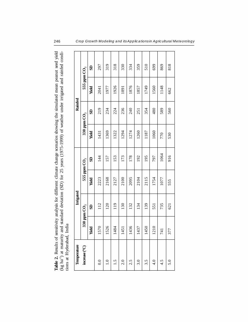
246 Crop Growth Modeling and its Applications in Agricultural Meteorology
Tab
le 2
. R
esul
ts o
f se
nsit
ivit
y an
alys
is f
or d
iffer
ent
clim
ate
chan
ge s
cena
rios
sho
win
g th
e si
mul
ated
mea
n pe
anut
see
d yi
eld
(kg
ha-1
) at
mat
urit
y an
d st
anda
rd d
evia
tion
(SD
) fo
r 25
yea
rs (
1975
-199
9) o
f w
eath
er u
nder
irr
igat
ed a
nd r
ainf
ed c
ondi
-ti
ons
at H
yder
abad
, In
dia
Tem
pera
ture
I
rrig
ated
R
ainf
ed
incr
ease
(o C)
330
ppm
CO
2
555
ppm
CO
2
330
ppm
CO
2
555
ppm
CO
2
Yiel
dSD
Yiel
dSD
Yiel
dSD
Yiel
dSD
0.0
1570
112
2223
144
1431
219
2041
297
1.0
1526
120
2168
157
1369
234
1977
319
1.5
1484
119
2127
153
1322
224
1926
318
2.0
1451
130
2100
173
1294
236
1891
330
2.5
1436
132
2095
178
1274
240
1876
334
3.0
1437
134
2104
192
1260
251
1857
359
3.5
1450
139
2115
195
1187
354
1749
510
4.0
1210
551
1754
797
1060
480
1560
699
4.5
741
735
1077
1064
770
589
1148
869
5.0
377
621
555
916
530
560
662
818

V. Radha Krishna Murthy 247
Tab
le 3
. R
esul
ts o
f se
nsit
ivit
y an
alys
is f
or d
iffer
ent
clim
ate
chan
ge s
cena
rios
sho
win
g th
e si
mul
ated
mea
n pe
anut
see
d yi
eld
(kg
ha-1)
at m
atur
ity
and
stan
dard
dev
iati
on (
SD)
for
25 y
ears
(19
75-1
999)
of w
eath
er u
nder
rai
nfed
con
diti
ons
at H
yder
abad
,In
dia
wit
h 20
% i
ncre
ase
or d
ecre
ase
in r
ainf
all
Tem
pera
ture
Rai
nfed
(+20
% r
ainf
all)
Rai
nfed
(-20
% r
ainf
all)
incr
ease
(o C)
3
30 p
pm C
O2
55
5 pp
m C
O2
3
30 p
pm C
O2
5
55 p
pm C
O2
Yiel
dSD
Yiel
dSD
Yiel
dSD
Yiel
dSD
0.0
1494
106
2140
129
1430
219
1948
354
1.0
1437
9520
6011
712
9829
418
7338
0
1.5
1400
8820
1811
412
5428
318
2137
8
2.0
1368
8219
9011
012
2229
517
8039
4
2.5
1356
8219
8012
211
9529
517
6241
6
3.0
1367
9320
0513
511
7731
517
4244
0
3.5
1385
106
2035
157
1095
394
1628
556
4.0
1346
301
1971
444
1015
452
1518
646
4.5
1238
475
1795
693
700
563
1048
830
5.0
1000
640
1213
1016
416
493
647
764

248 Crop Growth Modeling and its Applications in Agricultural Meteorology
site weather (soil and management) data also must be available. It is aknown fact that the weather data (and all these other details) are notavailable at all locations where crops are grown. To solve these problemsthe Geographical Information System (GIS) approach has opened up awhole field of crop modeling applications at spatial scale. From the fieldlevel for site-specific management to the regional level for productivityanalysis and food security the role of GIS is going to be tremendous(Hoogenboom, 2000).
APPLICATIONS AND USES OF CROP GROWTH MODELS INAGRICULTURAL METEOROLOGY
The crop growth models are being developed to meet the demands underthe following situations in agricultural meteorology.
1. When the farmers have the difficult task of managing their crops on poorsoils in harsh and risky climates.
2. When scientists and research managers need tools that can assist them intaking an integrated approach to finding solutions in the complex problemof weather, soil and crop management.
3. When policy makers and administrators need simple tools that can assistthem in policy management in agricultural meteorology.
The potential uses of crop growth models for practical applications are asfollows (Sivakumar and Glinni, 2000).
On farm decision-making and agronomic management
The models allow evaluation of one or more options that are available withrespect to one or more agronomic management decisions like:
Determine optimum planting date.
Determine best choice of cultivars.
Evaluate weather risk.
Investment decisions.
The crop growth models can be used to predict crop performance inregions where the crop has not been grown before or not grown under optimal
V. Radha Krishna Murthy 249
conditions. Such applications are of value for regional development andagricultural planning in developing countries (Van Keulen and Wolf, 1986).A model can calculate probabilities of grain yield levels for a given soil typebased on rainfall (Kiniry and Bockhot, 1998). Investment decisions likepurchase of irrigation systems (Boggess and Amerling, 1983) can be takenwith an eye on long term usage of the equipment thus acquired. Kiniry et al.(1991) showed that for maize, both simulated and measured mean yields withweeds are 86% of the weed-free yields.
Understanding of research
In agro-meteorological research the crop models basically helps in:
Testing scientific hypothesis.
Highlight where information is missing.
Organizing data.
Integrating across disciplines.
Assist in genetic improvement;
Evaluate optimum genetic traits for specific environments.
Evaluate cultivar stability under long term weather.
Penning de Vries (1977) emphasized that simulation models contributeto our understanding of the real system which in-turn helps to bridge areasand levels of knowledge. It is believed that in conversion of conceptual modelsinto mathematical simulation models the agrometeorologists can understandthe gaps in their knowledge. So, the interdisciplinary nature of simulationmodeling efforts leads to increased research efficacy and improved researchdirection through direct feedback. In this direction de Wit and Goudriaan(1978) developed BAsic CROp growth Simulator (BACROS) which was usedas a reference model for developing other models and as a basis for developingsummary models. Also O
Toole and Stockle (1987) described the potential of
simulation models in assessing trait benefits of winter cereals and their capacityto survive and reproduce in stress-prone environment. Crop growth modelshave been used in plant breeding to simulate the effects of changes in themorphological and physiological characteristics of crops which aid inidentification of ideotypes for different environments (Hunt, 1993; Kropffet al., 1995).
250 Crop Growth Modeling and its Applications in Agricultural Meteorology
Policy management
The policy management is one very useful application of crop simulationmodels. The issues range from global (impacts of climate change on crops) tofield level (effect of crop rotation on soil quality) issues. Thornton et al. (1997)showed that in Burkina Faso, crop simulation modeling using satellite andground-based data could be used to estimate millet production for famineearly warning which can allow policy makers the time they need to takeappropriate steps to ameliorate the effects of global food shortages on vulnerableurban and rural populations. In Australia Meinke and Hammer (1997) foundthat when November-December SOI (Southern Oscillation Index) phase ispositive, there is an 80% chance of exceeding average district yields. Conversely,in years when the November-December SOI phase is either negative or rapidlyfalling, there is only a 5% chance of exceeding average district yields, but a95% chance of below average yields. This information allows the industry toadjust strategically for the expected volume of production.
Crop models can be used to understand the effects of climate change suchas :
a) Consequences of elevated carbon-dioxide, and
b) Changes in temperature and rainfall on crop development, growth andyield. Ultimately, the breeders can anticipate future requirements basedon the climate change.
A FEW SUCCESSFULLY USED MODELS IN AGROMETEOROLOGY
Large scale evolution of computers since 1960 allowed to synthesizedetailed knowledge on plant physiological processes in order to explain thefunctioning of crops as a whole. Insights into various processes were expressedusing mathematical equations and integrated in simulation models. In thebeginning, models were meant to increase the understanding of crop behaviourby explaining crop growth and development in terms of the understandingphysiological mechanisms. Over the years new insights and different researchquestions motivated the further development of simulation models. In additionto their explanatory function, the applicability of well-tested models forextrapolation and prediction was quickly recognized and more application-oriented models were developed. For instance demands for advisory systemsfor farmers and scenario studies for policy makers resulted in the evolution ofmodels, geared towards tactical and strategic decision support respectively.
V. Radha Krishna Murthy 251
Now, crop growth modeling and simulation have become accepted tools foragricultural research.A few models used in agrometeorological studies are:
1. The de Wit school of models
In the sixties, the first attempt to model photosynthetic rates of cropcanopies was made (de Wit, 1965). The results obtained from this model wereused among others, to estimate potential food production for some areas ofthe world and to provide indications for crop management and breeding (deWit, 1967; Linneman et al., 1979). This was followed by the construction ofan Elementary CROp growth Simulator (ELCROS) by de Wit et al. (1970).This model included the static photosynthesis model and crop respiration wastaken as a fixed fraction per day of the biomass, plus an amount proportionalto the growth rate. In addition, a functional equilibrium between root andshoot growth was added (Penning de Vries et al., 1974). The introduction ofmicrometeorology in the models (Goudriaan, 1977) and quantification ofcanopy resistance to gas exchanges allowed the models to improve thesimulation of transpiration and evolve into the BAsic CROp growth Simulator(BACROS) (de Wit and Goudriaan, 1978).
2. IBSNAT and DSSAT Models
In many countries of the world, agriculture is the primary economicactivity. Great numbers of the people depend on agriculture for their livelihoodor to meet their daily needs, such as food. There is a continuous pressure toimprove agricultural production due to staggering increase in humanpopulation. Agriculture is very much influenced by the prevailing weather andclimate. The population increase is 2.1 per cent in India. This demands asystematic appraisal of climatic and soil resources to recast an effective landuse plan. More than ever farmers across the globe want access to options suchas the management options or new commercial crops. Often, the goal is toobtain higher yields from the crops that they have been growing for a longtime. Also, while sustaining the yield levels they want to :
1. Substantially improve the income.
2. Reduce soil degradation.
3. Reduce dependence on off-farm inputs.
4. Exploit local market opportunities.
252 Crop Growth Modeling and its Applications in Agricultural Meteorology
5. Farmers also need a facilitating environment in which;
a. Affordable credit is available.
b. Policies are conducive to judicious management of natural resources.
c. Costs and prices of production are stable.
6 Another key ingredient of a facilitating environment is information, suchas :
a. An understanding of which options are available.
b. How these operate at farm level.
c. The impact on issues of their priority.
To meet the above requirements of resource poor farmers in the tropicsand sub tropics IBSNAT (International Benchmark Sites Network for Agro-technology Transfer) began in 1982. This was under a contract from the U.S.Agency for International Development to the University of Hawaii at Manoa,USA. IBSNAT was an attempt to demonstrate the effectiveness ofunderstanding options through systems analysis and simulation for ultimatebenefit of farm households across the globe. The purposes defined for theIBSNAT project by its technical advisory committee were to :
1. Understand ecosystem processes and mechanisms.
2. Synthesize from an understanding of processes and mechanisms, a capacityto predict outcomes.
3. Enable IBSNAT clientele to apply the predictive capability to controloutcomes.
The models developed by IBSNAT were simply the means by which theknowledge scientists have and could be placed in the hands of users. In thisregard, IBSNAT was a project on systems analysis and simulation as a way toprovide users with options for change. In this project many researchinstitutions, universities, and researchers across the globe spent enormousamount of time and resources and focused on:
1 Production of a “decision support system” capable of simulating the risksand consequences of alternative choices, through multi-institute and multi-disciplinary approaches.
V. Radha Krishna Murthy 253
2. Definition of minimum amount of data required for running simulationsand assessing outcomes.
3. Testing and application of the product on global agricultural problemsrequiring site-specific yield simulations.
The major product of IBSNAT was a Decision Support System for Agro-Technology Transfer (DSSAT). The network members lead by J.W. Jones,Gainesville, USA developed this. The DSSAT is being used as a research andteaching tool. As a research tool its role to derive recommendations concerningcrop management and to investigate environmental and sustainability issuesis unparalleled. The DSSAT products enable users to match the biologicalrequirements of crops to the physical characteristics of land to provide themwith management options for improved land use planning. The DSSAT isbeing used as a business tool to enhance profitability and to improve inputmarketing.
The traditional experimentation is time consuming and costly. So, systemsanalysis and simulation have an important role to play in fostering thisunderstanding of options. The information science is rapidly changing. Thecomputer technology is blossoming. So, DSSAT has the potential to reducesubstantially the time and cost of field experimentation necessary for adequateevaluation of new cultivars and new management systems. Several crop growthand yield models built on a framework similar in structure were developed aspart of DSSAT package. The package consists of : 1) data base managementsystem for soil, weather, genetic coefficients, and management inputs, 2) Crop-simulation models, 3) series of utility programs, 4) series of weather generationprograms, 5) strategy evaluation program to evaluate options including choiceof variety, planting date, plant population density, row spacing, soil type,irrigation, fertilizer application, initial conditions on yields, water stress inthe vegetative or reproductive stages of development, and net returns.
Other Important Models
Crop models can be developed at various levels of complexity. The levelof complexity required depends on the objective of the modeling exercise. Thetop-down approach to model design (Hammer et al., 1989; Shorter et al.,1991) is appropriate for models aimed at yield prediction. In this approach,complexity is kept to a minimum by commencing with a simple frameworkand only incorporating additional phenomena or processes if they improve
254 Crop Growth Modeling and its Applications in Agricultural Meteorology
the predictive ability of the model. Sinclair (1986), Muchow et al. (1990)and Hammer and Muchow (1991) have adopted this method in developingmodels of soybean, maize and sorghum respectively.
The EPIC, ALAMANC, CROPSYST, WOFOST, ADEL models are beingsuccessfully used to simulate maize crop growth and yield. The SORKAM,SorModel, SORGF as also ALMANAC models are being used to address specifictasks of sorghum crop management. CERES – pearl millet model, CROPSYST,PmModels are being used to study the suitability and yield simulation of pearlmillet genotypes across the globe. Similarly, the two most common growthmodels used in application for cotton are the GOSSYM and COTONSmodels. On the same analogy the PNUTGRO for groundnut, CHIKPGROfor chick pea, WTGROWS for wheat, SOYGRO for soybean, QSUN forsunflower are in use to meet the requirements of farmers, scientists, decisionmakers, etc., at present. The APSIM, GROWIT added with several modulesare being used in crop rotation, crop sequence and simulation studies involvingperennial crops.
Under Indian sub-continent conditions, crop yield forecasting based onmeteorological data is very important from several points of view. Using cropyield as dependent variable and weather factors as independent variables,empirical statistical models for predicting crop yield have been reported byMall et al. (1996). Also, Mall and Gupta (2000) reported a successfulempirical statistical – yield weather model for wheat in the Varanasi districtof Uttar Pradesh, India. Rajesh Kumar et al. (1999) developed a stepwiseregression model which states that the pigeonpea yield variation by weathervariables is upto 94 per cent in Varanasi District, U.P., India. Using a thermaltime and phasic development model. Patel et al. (1999) found that pigeonpeaphenophases depended upon the available heat units and accounted for 98per cent of total variation in Anand, Gujarat State, India.
Elsewhere in the world there were studies (Robertson and Foong, 1977;Foong, 1981), which predicted yields based on climatic factors usingmathematical modeling. Factors such as water deficit, solar radiation, maximumand minimum temperatures which play a vital role at floral initiation weretaken into consideration to construct these models. In Southern Malaysia Ong(1982) found a high correlation between yield of oil palm and rainfall anddry spells as also temperature and sunshine using a step-wise regressionapproach. Chow (1991) constructed a statistical model for predicting crudepalm oil production with trend, season, rainfall, etc. Amissah-Arthur and Jagtap
V. Radha Krishna Murthy 255
(1995) successfully assessed nitrogen requirements by maize across agroecological zones in Nigeria using CERES-maize model. Hammer et al. (1995)using local weather and soil information correlated peanut yields with estimatesfrom PEANUTGRO, a model in the CERES family and gave a regression withhigh coefficient (r2 = 0.93) of variation. The construction of contemporarycrop models entails the combination of many algorithms for physiologicalprocesses and impact of environmental factors on process rates (Monteith,2000). This clearly indicates that in the development of models and theirapplication for solving problems at field level on agrometeorological aspectsare given due weightage.
APPLICATION OF MODELS IN AGRICULTURAL METEOROLOGY– PRECAUTIONS
Hunger demands food. Food grains come from agriculture, but it is risk-prone. So research efforts are necessary. Unfortunately, funding for researchworldwide is declining at an alarming rate. The agricultural scientists andplanners are facing formidable challenges to ensure continued increases inagricultural productivity to meet the food grain requirements of burgeoningpopulation across the globe. Nowadays, the traditional field experimentationis becoming very expensive. So, the works on development and use of cropgrowth models to answer strategic and tactical questions concerning agriculturalplanning as well as on-farm soil and crop management are essential.
Although these models are useful in more than one way as detailed earlierin this lecture, much of the modeling uses and applications to date have beenmainly in the area of research. The products of research need to bedisseminated to the farmers. Otherwise the present works on crop modelingcannot sustain in the long run. So far, much of crop modeling applications inthe literature are based on sole cropping and only in the recent past this workhas been extended to intercrops, crop rotations, crop sequences, etc. The workson crop rotations shall be taken up on priority. If one considers the attentiongiven to individual crops so far maize and cotton rank more than 50% of thework but there are many other crops that meet food requirements of thepopulation in tropical and sub-tropical areas of the world. So, it is essentialto understand fully the physical and physiological processes of these crops thatgovern their growth and yield under valuable soil and climatic conditionsthrough crop models.
The development of agrometerological and agroclimatological modelsinclude climate crop and soil. The availability of water (which is an observed
256 Crop Growth Modeling and its Applications in Agricultural Meteorology
parameter through rainfall) and water requirement (expressed by PET whichis an estimated parameter) are basic inputs in majority of these studies. Thesuitability of individual models for the estimation of PET depends not onlyon accurate predictive ability of the model but also on the availability ofnecessary input data. In addition, the following points shall be taken intoconsiderations in model development and their application as precautions inagricultural meteorological studies.
1. Adequate human resource capacity has to be improved to develop andvalidate simulation models across the globe.
2. Multi-disciplinary research activities are essential for qualitative works incrop growth modeling.
3. Linkages shall be made and strengthened among research – education –extension to quickly disseminate the outcomes of models to farmers.
4. Majority of models use rainfall data at monthly interval, which is too longa period when compared to short duration of dry land crops (Sorghum,pearlmillet mature in 100 days). So, there is an urgent need to correctthis anomaly by selecting proper methodologies.
5. It is important to differentiate between models of interest for research andfor practical application. So, models useful to farmers with minimum inputparameters shall find right place in the society.
6. It is always preferable to use one or more methods / models in conjunctionto get more realistic conclusions useful to the farmers, who are the ultimatebeneficiary alongwith industries.
7. The requirements in terms of details for local agricultural planning andoperations are quite different from regional agricultural planning.Therefore, while selecting / using any model, it must be kept in mindthe clear objective of study on one hand and verifying with ground truth(irrespective of the claims of the modal author) on the other hand.
8. The results / output of the models must be interpreted in an appropriateway by integrating soil, weather and crop. This interpretation is the keyfor success of agrometerological models. So, application of crop growthmodels shall form a part of studies of agrometeorologists on a regular andmore continuous basis.
V. Radha Krishna Murthy 257
9. One should trust contemporary models particularly those concerned withyields. Wide variations may be found in the yield predicted by differentmodels for specific crop in a defined environment. There is a need todevelop test and improve the models with similar basis till they achievecomparable success for use by farmers, extension workers industry, etc.The reason is that the farmer needs them for decision-making, because Itwas found that the model can be used to identity new sites suitable fordevelopment of crop which finally results in generation of income to them.
10. It will be important to link the crop simulation models to local short andlong-term weather forecasts. This will improve the yield predictions andprovide policy makers with advanced yield information to help manageexpected famines and other associated problems.
CONCLUSIONS
Various kinds of models such as Statistical, Mechanistic, Deterministic,Stochastic, Dynamic, Static, Simulations are in use for assessing and predictingcrop growth and yield. Crop growth model is a very effective tool for predictingpossible impacts of climatic change on crop growth and yield. Crop growthmodels are useful for solving various practical problems in agriculture.Adequate human resource capacity has to be improved to be develop andvalidate simulation models across the globe.
ACKNOWLEDGEMENTS
The author wishes to acknowledge the excellent encouragement, technicalreview and recommendations provided by Dr. M.V.K. Sivakumar, ProfessorC.J. Stigter, Professor Gerrit Hoogenboom and Dr. P.V.V. Prasad in preparationof the manuscript.
REFERENCES
Allen, L.H., Valle, P.R., Jones, J.W. and Jones, P.H. 1998. Soybean leaf water potentialresponses to carbon dioxide and drought. Agronomy Journal 90: 375-383.
Amissah-Arthur, A. and Jagtap, S.S. 1995. Application of models and geographic informationsystem based decision support system in analysis the effect of rainfall on maize yieldstability. Sustain Africa 3: 2-15.
258 Crop Growth Modeling and its Applications in Agricultural Meteorology
Boggess, W.G. and Amerling, C.B. 1983. A bioeconomic simulation analysis of irrigationenvironments. S.J. Agric. Econ. 15: 85-91.
Boote, K.J., Jones, J.W., Hoogenboom, G., Wilkerson, G.G. and Jagtap, S.S. 1989.PNUTGRO VI.0, Peanut crop growth simulation model, user’s guide. FloridaAgricultural Experiment Station, Journal No. 8420. University of Florida, Gainesville,Florida, USA.
Chow, C.S. 1991. Seasonal and rainfall effects on oil palm yield in Malaysia. Second NationalSeminar on Agrometeorology, Petaling Jaya, Malaysia, pp. 109-128.
Clifford, S.C., Stronach, I.M., Black, C.R., Singleton-Jones, P.R., Azam-Ali, S.N. and Crout,N.M. 2000. Effects of elevated CO
2, drought and temperature on the water relations
and gas exchange of groundnut (Arachis hypogaea L.) stands grown in controlledenvironment glasshouses. Physiological Plantarum 110: 78-88.
de Wit, C.T. and J. Goudriaan. 1978. Simulation of assimilation, respiration and transpirationof crops. Simulation monograph. PUDOC, Wageningen, The Netherlands.
de Wit, C.T., R. Brouwer and F.W.T. Penning de Vries. 1970. The simulation ofphotosynthetic systems, in prediction and measurement of photosynthetic productivity.Proceedings of International Biological Program/Plant Production Technical Meeting.Setlik, I., Ed., Trebon, PUDOC, Wageningen, The Netherlands.
de Wit, C.T. 1965. Photosynthesis of leaf canopies. Agricultural Research Report No. 663.PUDOC, Wageningen, The Netherlands.
de Wit, C.T. 1967. Photosynthesis: its relationship to overpopulation. p. 315-320. InHarvesting the sun. Academic Press, New York.
Foong, S.F. 1981. An improved weather model for estimating oil palm fruit yield. The OilPalm in Agriculture in the Eighties. ISP, Malaysia.
Goudriaan, J. 1977. Crop micrometeorology: a simulation study. Simulation monograph.PUDOC. Wageningen, The Netherlands.
Hammer, G.L., Hoizworth, D.P., Mulo, S. and Wade, L.J. 1989. Modeling adaptation andrisk of production of grain sorghum in Australia. p. 257-267. In M.A., Foale, B.W.Hare and R.G. Henzell (eds.) Proc. of the Australian Sorghum Workshop, Too-woomba.28 Feb.-1 Mar. 1989. Australian Institute of Agricultural Science, Brisbane.
Hammer, G.L. and Muchow, R.C. 1991. Quantifying climatic risk to sorghum in Australia’ssemiarid tropics and subtropics : Model development and simulation. p. 205-232. In R.C.Muchow and J.A. Bellamy (eds.) Climatic risk in crop production : models and managementfor the semiarid tropics and subtropics. C.A.B. International, Wallingford, UK.
V. Radha Krishna Murthy 259
Hammer, G.L., Sinclair, T.R., Boote, K.J., Wright, G.C., Meinke, H. and Bell, M.J. 1995. Apeanut simulation model. 1. Model development and testing. Agron. J. 87: 1085-1093.
Hoogenboon, G. 2000. Contribution of agrometeorology to the simulation of cropproduction and its applications. Agril. and For. Meteorol. 103 : 137-157.
Hunt, L.A. 1993. Designing improved plant types: a breeders view point. p. 3-17. In F.W.T.Penning de Vries et al. (ed.) Systems approaches for sustainable agricultural development.Kluwer Academic Publishers, Dordrecht, The Netherlands.
ICAR 2000. Crop Statistics Reports. Indian Council of Agricultural Research, New Delhi,India.
Kiniry, J.R. and A.J. Bockholt 1998. Maize and sorghum simulation in diverse Texasenvironments. Agron. J. 90: 682-687.
Kiniry, J.R., W.D. Rosenthal, B.S. Jackson and G. Hoogenboom. 1991. Predicting leafdevelopment of crop plants. p.29-42. In T. Hodges (ed.) Predicting Crop Phenology.CRC Press, Boca Raton, FL.
Kropff, M.J., A.J. Haverkort, P.K. Aggarwal and P.L. Kooman. 1995. Using systemsapproaches to design and evaluate ideotypes for specific environments. p. 417-435. InJ. Bouma, A. Kuyvenhoven, B.A.M. Bouman, J.C. Luyten and H.G. Zandstra (eds.)Eco-regional approaches for sustainable land use and food production. Kluwer AcademicPublishers, Dordrecht, The Netherlands.
Linneman, H., J. Dehoogh, M.A. Keyzer and H.D.J. van Heemst. 1979. Moira, model ofinternational relations in agriculture. North Holland Publishing Company, Amsterdam.
Long, S.P., Baker, N.R. and Raines, C.A. 1993. Analysing responses of photosyntheticacclimation to long elevation of atmospheric CO
2 concentration. Vegetatio 104/104 :
33-45.
Mall, R.K. 1996. Some agrometeorological aspects of wheat crop and development of yieldforecast models. Ph.D thesis (unpublished), Banaras Hindu University, Varanasi, India.
Meinke, H. and G.L. Hammer. 1997. Forecasting regional crop production using SOI phases :an example for the Australian peanut industry. Aust. J. Agric. Res. 48: 789-793.
Monteith, J.L. 2000. Agricultural meteorology: Evolution and application. Agri. For.Meteorol. 103(2000) 5-9.
Morrison, J.I.L. and Lawlor, D.W. 1999. Interactions between increasing CO2 concentration
and temperature on plant growth. Plant Cell and Environment 22 : 659-682.
260 Crop Growth Modeling and its Applications in Agricultural Meteorology
Muchow, R.C., Sinclair, T.R. and Bennett, J.M., 1990. Temperature and solar radiation effectson potential maize yield across locations. Agron. J. 82 : 338-343.
Murthy, V.R.K. 1999. Studies on the influence of macro and micro meteorological factorson growth and yield of soybean. Unpublished Ph.D thesis submitted to ANGRAU,Hyderabad, India.
Murthy, V.R.K. 2002. Basic principles of Agricultural Meteorology. Book syndicate publishers,Koti, Hyderabad, India.
Ong, H.T. 1982. System approach to climatology of oil palm. 1. Identification of rainfalland dry spell aspects 2. Identification of temperature and sunshine. Oleagineux 37,93,-443.
O’Toole, J.C. and C.O. Stockle. 1987. The role of conceptual and simulation modelling inplant breeding. Presented at the Int. Symp. on Improving Winter Cereals underTemperature and Soil Salinity Stresses, 26-29 October 1987, Cordoba, Spain.
Patel, H.R., Shekh, A.M., Bapuji Rao, B., Chaudhari, G.B. and Khushu, M.K. 1999. J. ofAgromet. 1(2) : 149-154.
Penning de Vries, F.W.T. 1977. Evaluation of simulation models in agriculture and biology:conclusions of a workshop. Agricultural Systems 2: 99-105.
Penning de Vries, F.W.T., A.B. Brunsting and H.H.van Laar, 1974. Products, requirementsand efficiency of biological synthesis, a quantitative approach. J. Theor. Biol. 45: 339-377.
Robertson, G.W. and Foong, S.F. 1977. Weather-based yield forecasts for oil palm freshfruit bunches. International Development in Oil Palm, ISP, Kuala Lumpur.
Shorter, R., Lawn, R.J. and Hammer, G.L. 1991. Improving genotypic adaptation in crops– a role for breeders, physiologists and modelers. Exp. Agric. 27 : 155-175.
Sinclair, T.R. 1986. Water and nitrogen limitations in soybean grain production. I. Modeldevelopment. Field Crops Res. 15 : 125-141.
Sivakumar, M.V.K. and Glinni, A.F. 2002. Applications of crop growth models in the semi-arid regions. pages 177-205. In Agricultural System Models in Field Research andTechnology Transfer (Eds. L.R. Ahuja, L. Ma and T.A. Howell), Lewis Publishers, ACRC Press Company, Boca Raton, USA.
Sivakumar, M.V.K., Gommes, R. and Baier, W. 2000. Agrometeorology and sustainableagriculture. Agric. and For. Meteorol. 103: 11-26.

V. Radha Krishna Murthy 261
Thornton, P.K., W.T. Bowen, A.C. Ravelo, P.W. Wilkens, G. Farmer, J. Brock and J.E. Brink.1997. Estimating millet production for famine early warning: an application of cropsimulation modelling using satellite and ground-based data in Burkina Faso. Agriculturaland Forest Meteorology 83: 95-112.
Unsworth, M.H. and Hogsett, W.E. 1996. Combined effects of changing CO2, temperature,
UV-B radiation on crop growth. pp. 171-197. In Global climate change and agriculturalproduction; direct and indirect effects of changing hydrological, pedological and plantphysiological processes (Eds. F. Bazzaz and W. Sombroek). Food and AgriculturalOrganization, Rome and John Wiley and Sons, West Sussex, England.
Van Keulen, H. and Wolf, J. (ed). 1986. Modelling of agricultural production: weather,soils and crops. Simulation Monographs. PUDOC, Wageningen, The Netherlands.
CROP GROWTH AND PRODUCTIVITYMONITORING AND SIMULATION USINGREMOTE SENSING AND GIS
V.K. Dadhwal*Crop Inventory and Modelling Division, ARGSpace Applications Centre (ISRO)Ahmedabad
Abstract: Crop growth and productivity are determined by a large number ofweather, soil and management variables, which vary significantly across space. RemoteSensing (RS) data, acquired repetitively over agricultural land help in identificationand mapping of crops and also in assessing crop vigour. As RS data and techniqueshave improved, the initial efforts that directly related RS-derived vegetation indices(VI) to crop yield have been replaced by approaches that involve retrieved biophysicalquantities from RS data. Thus, crop simulation models (CSM) that have beensuccessful in field-scale applications are being adapted in a GIS framework to modeland monitor crop growth with remote sensing inputs making assessments sensitiveto seasonal weather factors, local variability and crop management signals. The RSdata can provide information of crop environment, crop distribution, leaf area index(LAI), and crop phenology. This information is integrated in CSM, in a number ofways such as use as direct forcing variable, use for re-calibrating specific parameters,or use simulation-observation differences in a variable to correct yield prediction.A number of case studies that demonstrated such use of RS data and demonstrated
applications of CSM-RS linkage are presented.
INTRODUCTION
Crop growth and yield are determined by a number of factors such asgenetic potential of crop cultivar, soil, weather, cultivation practices (date ofsowing, amount of irrigation and fertilizer) and biotic stresses. However,generally for a given area, year-to-year yield variability has been mostly modeled
Satellite Remote Sensing and GIS Applications in Agricultural Meteorologypp. 263-289
(* Present Address : Indian Institute of Remote Sensing, Dehra Dun 248 001, India;email: [email protected])
264 Crop Growth and Productivity Monitoring and Simulation
through weather as a predictor using either empirical or crop simulationapproach. With the launch and continuous availability of multi-spectral(visible, near-infrared) sensors on polar orbiting earth observation satellites(Landsat, SPOT, IRS, etc) remote sensing (RS) data has become an importanttool for yield modeling. RS data provide timely, accurate, synoptic andobjective estimation of crop growing conditions or crop growth for developingyield models and issuing yield forecasts at a range of spatial scales. RS datahave certain advantage over meteorological observations for yield modeling,such as dense observational coverage, direct viewing of the crop and ability tocapture effect of non-meteorological factors. Recent developments in GIStechnology allow capture, storage and retrieval and visualization and modelingof geographically linked data. An integration of the three technologies, viz.,crop simulation models, RS data and GIS can provide an excellent solutionto monitoring and modeling of crop at a range of spatial scales.
In this paper an attempt is made to introduce a basic framework andindicate through specific case studies, (a) how RS data are useful in estimatingcrop parameters like LAI, (b) introduce crop simulation models, (c) how GIStools are used for crop monitoring with RS data and interfaced with models,and (d) how RS-derived parameters, crop simulation models and GIS are usefulfor crop productivity modeling. Details on some of the above topics can beobtained from recent reviews, such as Moulin et al. (1998), Dadhwal (1999),Hartkamp et al. (1999), Dadhwal and Ray (2000), Maracchi et al. (2000)and Dadhwal et al. (2003).
LAI estimation using RS-data
The leaf area index (LAI), defined, as the total one-sided leaf area per unitground area, is one of the most important parameters characterizing a canopy.Because LAI most directly quantifies the plant canopy structure, it is highlyrelated to a variety of canopy processes, such as evapotranspiration, lightinterception, photosynthesis, respiration and leaf litterfall. RS-based LAIestimation would greatly aid the application of LAI as input to models ofphotosynthesis, crop growth and yield simulation models, evapotranspiration,estimation of net primary productivity and vegetation/ biosphere functioningmodels for large areas. A number of techniques for space borne remote sensingdata have been developed/tested, ranging from regression models to canopyreflectance model inversions with varying successes, which include (1) statisticalmodels that relate LAI to band radiance (Badhwar et al., 1986) or developLAI-vegetation index relation (Chen and Cihlar, 1996 and Myneni et al.,
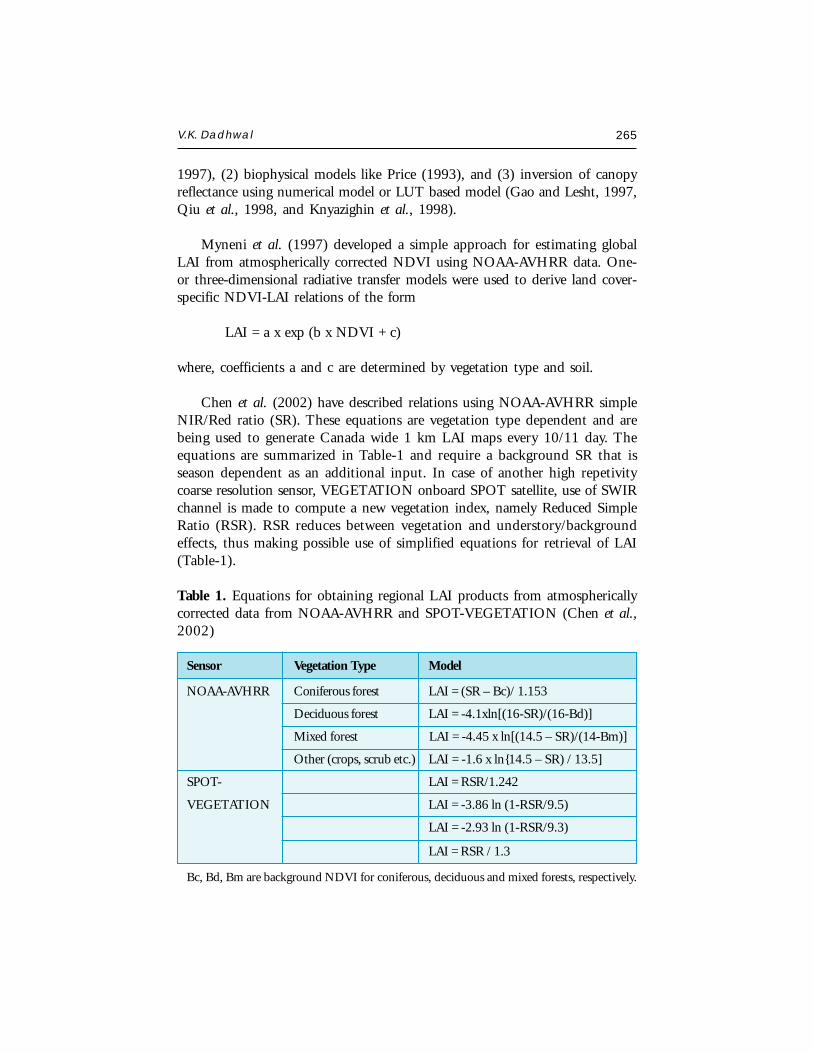
V.K. Dadhwal 265
1997), (2) biophysical models like Price (1993), and (3) inversion of canopyreflectance using numerical model or LUT based model (Gao and Lesht, 1997,Qiu et al., 1998, and Knyazighin et al., 1998).
Myneni et al. (1997) developed a simple approach for estimating globalLAI from atmospherically corrected NDVI using NOAA-AVHRR data. One-or three-dimensional radiative transfer models were used to derive land cover-specific NDVI-LAI relations of the form
LAI = a x exp (b x NDVI + c)
where, coefficients a and c are determined by vegetation type and soil.
Chen et al. (2002) have described relations using NOAA-AVHRR simpleNIR/Red ratio (SR). These equations are vegetation type dependent and arebeing used to generate Canada wide 1 km LAI maps every 10/11 day. Theequations are summarized in Table-1 and require a background SR that isseason dependent as an additional input. In case of another high repetivitycoarse resolution sensor, VEGETATION onboard SPOT satellite, use of SWIRchannel is made to compute a new vegetation index, namely Reduced SimpleRatio (RSR). RSR reduces between vegetation and understory/backgroundeffects, thus making possible use of simplified equations for retrieval of LAI(Table-1).
Table 1. Equations for obtaining regional LAI products from atmosphericallycorrected data from NOAA-AVHRR and SPOT-VEGETATION (Chen et al.,2002)
Sensor Vegetation Type Model
NOAA-AVHRR Coniferous forest LAI = (SR – Bc)/ 1.153
Deciduous forest LAI = -4.1xln[(16-SR)/(16-Bd)]
Mixed forest LAI = -4.45 x ln[(14.5 – SR)/(14-Bm)]
Other (crops, scrub etc.) LAI = -1.6 x ln{14.5 – SR) / 13.5]
SPOT- LAI = RSR/1.242
VEGETATION LAI = -3.86 ln (1-RSR/9.5)
LAI = -2.93 ln (1-RSR/9.3)
LAI = RSR / 1.3
Bc, Bd, Bm are background NDVI for coniferous, deciduous and mixed forests, respectively.
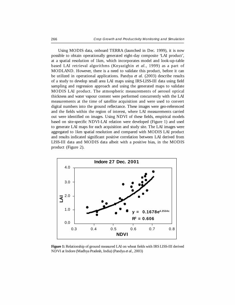
266 Crop Growth and Productivity Monitoring and Simulation
Using MODIS data, onboard TERRA (launched in Dec. 1999), it is nowpossible to obtain operationally generated eight-day composite ‘LAI product’,at a spatial resolution of 1km, which incorporates model and look-up-tablebased LAI retrieval algorithms (Knyazighin et al., 1999) as a part ofMODLAND. However, there is a need to validate this product, before it canbe utilized in operational applications. Pandya et al. (2003) describe resultsof a study to develop small area LAI maps using IRS-LISS-III data using fieldsampling and regression approach and using the generated maps to validateMODIS LAI product. The atmospheric measurements of aerosol opticalthickness and water vapour content were performed concurrently with the LAImeasurements at the time of satellite acquisition and were used to convertdigital numbers into the ground reflectance. These images were geo-referencedand the fields within the region of interest, where LAI measurements carriedout were identified on images. Using NDVI of these fields, empirical modelsbased on site-specific NDVI-LAI relation were developed (Figure 1) and usedto generate LAI maps for each acquisition and study site. The LAI images wereaggregated to 1km spatial resolution and compared with MODIS LAI productand results indicated significant positive correlation between LAI derived fromLISS-III data and MODIS data albeit with a positive bias, in the MODISproduct (Figure 2).
Figure 1: Relationship of ground measured LAI on wheat fields with IRS LISS-III derivedNDVI at Indore (Madhya Pradesh, India) (Pandya et al., 2003)
Indore 27 Dec. 2001
LAI
4.0
3.0
2.0
1.0
0.0
0.3 0.4 0.5 0.6 0.7 0.8NDVI
y = 0.1678e4.2534x
R2 =0.606
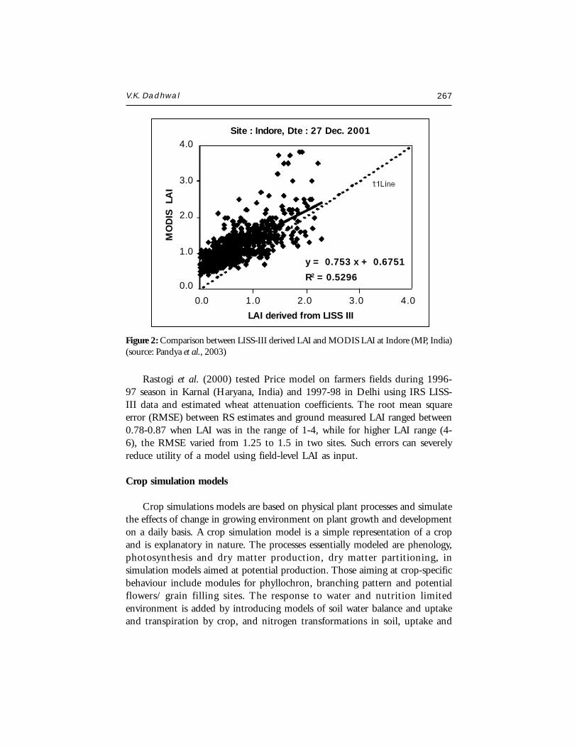
V.K. Dadhwal 267
Rastogi et al. (2000) tested Price model on farmers fields during 1996-97 season in Karnal (Haryana, India) and 1997-98 in Delhi using IRS LISS-III data and estimated wheat attenuation coefficients. The root mean squareerror (RMSE) between RS estimates and ground measured LAI ranged between0.78-0.87 when LAI was in the range of 1-4, while for higher LAI range (4-6), the RMSE varied from 1.25 to 1.5 in two sites. Such errors can severelyreduce utility of a model using field-level LAI as input.
Crop simulation models
Crop simulations models are based on physical plant processes and simulatethe effects of change in growing environment on plant growth and developmenton a daily basis. A crop simulation model is a simple representation of a cropand is explanatory in nature. The processes essentially modeled are phenology,photosynthesis and dry matter production, dry matter partitioning, insimulation models aimed at potential production. Those aiming at crop-specificbehaviour include modules for phyllochron, branching pattern and potentialflowers/ grain filling sites. The response to water and nutrition limitedenvironment is added by introducing models of soil water balance and uptakeand transpiration by crop, and nitrogen transformations in soil, uptake and
Figure 2: Comparison between LISS-III derived LAI and MODIS LAI at Indore (MP, India)(source: Pandya et al., 2003)
Site : Indore, Dte : 27 Dec. 2001
LAI derived from LISS III
MO
DIS
LA
I
4.0
3.0
2.0
1.0
0.0
0.0 1.0 2.0 3.0 4.0
y = 0.753 x + 0.6751
R2 =0.5296
268 Crop Growth and Productivity Monitoring and Simulation
remobilization within plant, respectively. Models of effects of weeds and pestsare being developed and could be available in new generation of crop simulationmodels.
In dynamic crop simulation models, three categories of variables recognizedare, state, rate and driving variables. The state variables are quantities likebiomass, amount of nitrogen in soil, plant, soil water content, which can bemeasured at specific times. Driving variables, or forcing functions, characterizethe effect of the environment on the system at its boundaries, and their valuesmust be monitored continuously, e.g., meteorological variables. Each statevariable is associated with rate variables that characterize their rate of changeat a certain instant as a result of specific processes. These variables representflow of material or biomass between state variables. Their value depends onthe state and driving variables according to rules that are based on knowledgeof the physical, chemical and biological processes that take place during cropgrowth.
Under the International Benchmark Sites Network for AgrotechnologyTransfer (IBSNAT) project a computer software package called the DecisionSupport System for Agrotechnology Transfer (DSSAT) was developed whichintegrates 11 crop simulation models (CERES cereal, CROPGRO legume andother models) with a standardized input and output (Jones, 1993) and hasbeen evaluated/ used in a number of countries. Use of CERES-Wheat includedin DSSAT for regional wheat yield prediction has been demonstrated recentlyin India (Nain et al., 2004).
GIS AND ITS USE FOR CROP MONITORING
Introduction to GIS
Burrough and McDonnell (1998) has defined GIS as a powerful set oftools for collecting, storing, retrieving at will, transforming and displayingspatial data from the real world for a particular set of purposes. The threemajor components of GIS are (i) computer hardware, (ii) computer softwareand (ii) digital geographic data. The information stored within a GIS is oftwo distinct categories. The spatially referenced information that can berepresented by points, lines, and polygons, that are referenced to a geographiccoordinate system and is usually stored in either raster (grid-cell) or vector(arc-node) digital format. The second category of information stored in a GISis attribute data or information describing the characteristics of the spatialfeature.
V.K. Dadhwal 269
Using RS & GIS for crop monitoring
The use of GIS along with RS data for crop monitoring is an establishedapproach in all phases of the activity, namely preparatory, analysis and output.In the preparatory phase GIS is used for (a) stratification/zonation using oneor more input layers (climate, soil, physiolgraphy, crop dominance etc.), or(b) preparing input data (weather, soil and collateral data) which is availablein different formats to a common format. In the analysis phase use of GIS ismainly through operations on raster layers of NDVI or computing VI profileswithin specified administrative boundaries. The final output phase also involvesGIS for aggregation and display of outputs for defined regions (e.g.,administrative regions) and creating map output products with required dataintegration through overlays.
Wade et al. (1994) described efforts within National Agricultural StatisticsService (NASS) of U.S. Department of Agriculture (USDA) of using NOAAAVHRR NDVI for crop monitoring and assessment of damage due to floodand drought by providing analysts a set of map products. Combining satellitedata in a GIS can enhance the AVHRR NDVI composite imagery byoverlaying State and county boundaries. The use of raster-based (grid-cell)capabilities of ARC/INFO (GRID) for the generation of difference image helpscompare a season with previous year or average of a number of years. Overlayinga crop mask helps in highlighting only effects on crops. Application of frostisolines is made to help analysts to locate average dates of the first frost forpossible crop damage. Generation and overlay of contours of precipitation datagenerated using TIN function of ARC/INFO also is an aid to interpretingNDVI difference image.
Interfacing crop simulation models to GIS
Crop simulation models, when run with input data from a specific field/site, produce a point output. The scope of applicability of these simulationmodels can be extended to a broader scale by providing spatially varying inputs(soil, weather, crop management) and policy combining their capabilities witha Geographic Information System (GIS). The main purpose of interfacingmodels and GIS is to carry out spatial and temporal analysis simultaneouslyas region-scale crop behaviour has a spatial dimension and simulation modelsproduce a temporal output. The GIS can help in spatially visualizing the resultsas well as their interpretation by spatial analysis of model results.
270 Crop Growth and Productivity Monitoring and Simulation
While GIS and modeling tools have existed for so long, the integration,including the conceptual framework is being given attention only recently.Hartkamp et al. (1999) have reviewed GIS and agronomic modeling andsuggested that ‘interface’ and ‘interfacing’ be used as umbrella words forsimultaneously using GIS and modeling tools, and ‘linking’, ‘combining’ and‘integrating’ as suitable terminology for degree of interfacing. These correspondto loose, tight and embedded coupling, respectively, as used by Burrough(1996) and Tim (1996). While there is a continuum between linking andcombining, the terms are explained below:
(a) Linking: Simple linkage strategies use GIS for spatially displaying modeloutputs. A simple approach is interpolation of model outputs. An advancedstrategy is to use GIS functions (interpolation, overlay, slope, etc.) toproduce a database containing inputs of the model and model outputsare also exported to the same database. Communication between GIS andmodel is through identifiers of grid cells or polygons in input and outputfiles, which are transferred in ascii or biary format between GIS and model(Figure 3a). Such an approach is not able to utilize full potential of thesystem and suffers from limitation due to (a) dependence on formats ofGIS and model, (b) incompatibility of operating environments and (c)not fully utilizing the capabilities of GIS.
(b) Combining: Combining also involves processing data in a GIS anddisplaying model results, however, the model is configured with GIS anddata are exchanged automatically. This is done with facilities in GIS packageof macro language, interface programmes, libraries of user callable routines(Figure 3b). This requires more complex programming and datamanagement than simple linking. Example of combining is AEGIS(Agricultural and Environmental GIS) with ArcView (Engel et al., 1997).
(c) Integrating: Integration implies incorporating one system into the other.Either a model is embedded in GIS or a GIS system is included in amodeling system. This allows automatic use of relational database andstatistical packages (Figure 3c). This requires considerable expertise, effortand understanding of the two tools.
Calixte et al. (1992) developed a regional agricultural decision supportsystem, known as Agricultural and Environmental Geographic informationSystem (AEGIS) that uses the DSSAT capabilities within ARC/INFO GIS forregional planning and productivity analysis. AEGIS allows the user to select
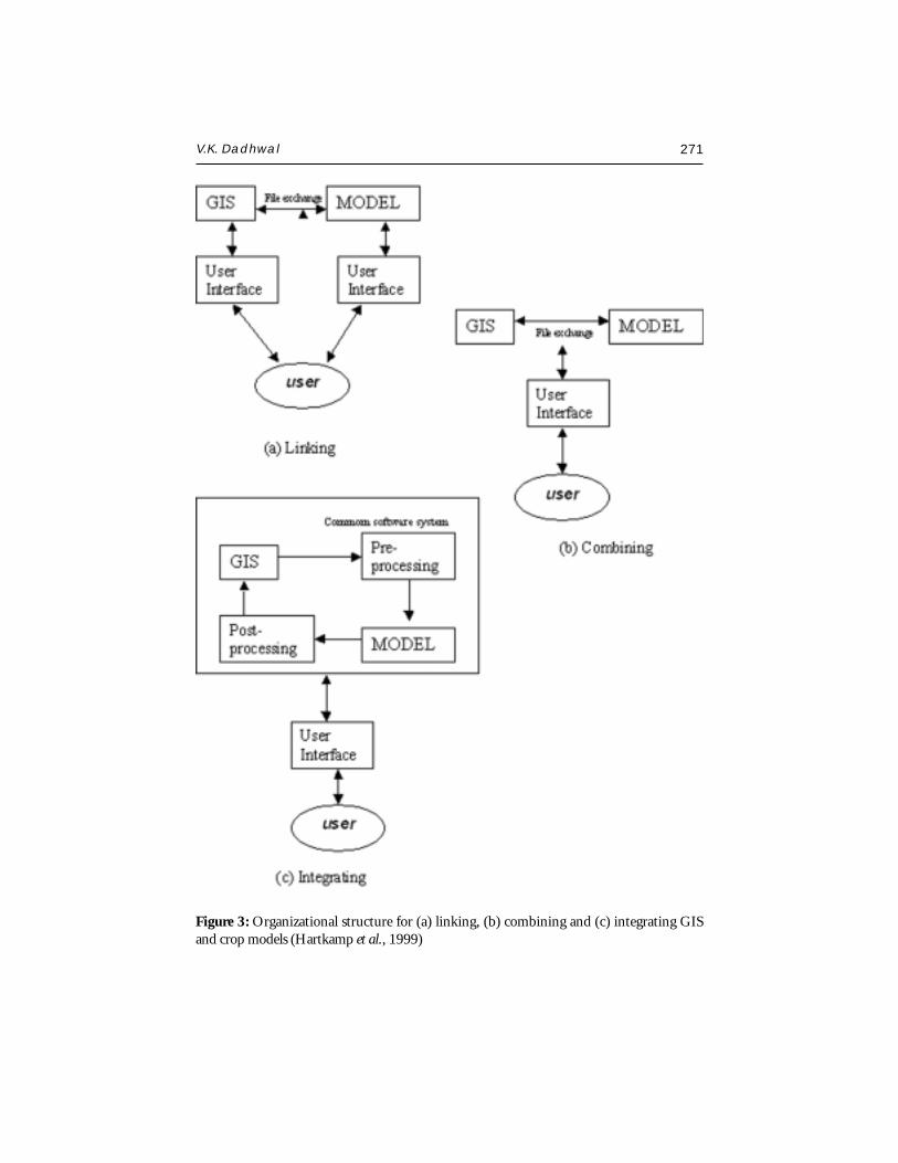
V.K. Dadhwal 271
Figure 3: Organizational structure for (a) linking, (b) combining and (c) integrating GISand crop models (Hartkamp et al., 1999)
272 Crop Growth and Productivity Monitoring and Simulation
various combinations of crop management practices over space and evaluatepotential crop production. Engel et al. (1997) modified the AEGIS intoAEGIS/WIN (AEGIS for Windows) written in Avenue, an object-orientedmacro scripting language, which links the DSSAT (Version 3) with thegeographical mapping tool ArcView-2. Thornton et al. (1997a) developedspatial analysis software for the most recent release of the DSSAT, Version 3.1.This software standardized the links between crop models and GIS softwareand this allowed developers to make use of whatever GIS software is mostsuitable for a particular purpose, while ensuring that basic links to the DSSATsystem and the crop models are the same. The spatial analysis software hastwo modules: (i) a geostatistical module to interpolate maps and produceprobability surfaces from a network of data points, and (ii) a utility thatcalculates agronomic and economic output statistics from model simulationsand maps the results as polygons. Another effort is development of a SPATIAL-EPIC linked to Arc/Info (Satya et al., 1998).
Demonstrated applications of CSM interfaced with GIS
Current wide range of applications of interfacing of GIS and modellingare reviewed by Hartkamp et al. (1999) and covers spatial yield calculation(regional and global), precision farming, climate change studies, and agro-ecological zonation, etc.
CGMS (Crop Growth Monitoring System) of MARS (Monitoring Agriculture withRemote Sensing)
This project of European Union uses WOFOST model and Arc/Info foroperational yield forecasting of important crops (Meyer-Roux and Vossen,1994). The Crop Growth Monitoring System (CGMS) of the MARS integratescrop growth modelling (WOFOST), relational batabase ORACLE and GIS(ARC/INFO) with system analytical part for yield forecasting (Bouman et al.,1997). There are databases on soil, weather, crop, and yield statistics that coverthe whole of EU. The system-analytical part consists of three modules:agrometeorological module, a crop growth module and a statistical module.The meteorological module takes care of the processing of daily meteorologicaldata that are received in real time to a regular grid of 50x50 km for use asinput by crop growth model or for assessment of ‘alarm’ conditions. The cropgrowth module consists of the dynamic simulation model WOFOST in whichcrop growth is calculated and crop indicators are generated for two productionlevels: potential and water-limited. In CGMS, WOFOST is run on a dailybases for each so-called ‘simulation unit’, i.e. a unique combination of weather,
V.K. Dadhwal 273
soil, and crop (mapping) units. In the statistical module, crop indicators (totalabove ground dry weight and dry weight storage organs) calculated withWOFOST are related to historical yield statistics through regression analysisin combination with a time-trend, for at least 15 years of simulated andhistorical data (Vossen, 1995). The resulting regression equations per crop perregion are used to make actual yield forecast. CGMS generates on a 10 dayand monthly basis three types of output on current cropping season: (i) Mapsof accumulated daily weather variables on 50x50 km grid to detect anyabnormalities, e.g. drought, frost, (ii) Maps of agricultural quality indicatorsbased on comparison of simulated crop indicators with their long-term means,(iii) Maps and tables of yield forecasts.
Precision Farming
Han et al. (1995) developed an interface between PC ARC/INFO GISand SIMPOTATO simulation model to study potato yield and N leachingdistribution for site-specific crop management (precision farming) in a 50 hafield. The GIS input layers, corresponding to important distributed inputparameters for the model, were irrigated water/N layer, soil texture layers andinitial soil N layers. For each unique sub-area stored in the GIS database, theinterface program extracts the attribute codes of that sub-area from the GISdatabase, converts the attribute codes to the input parameters of theSIMPOTATO and sends them to the model. After running the model, theinterface program retrieves the output data (potato yield and N leaching),converts them to the attribute codes and stores the output data in the GISdatabase.
Agro-ecological Zonation
Aggarwal (1993) used WTGROWS to simulate potential and water-limitedwheat yields for 219 weather locations spread all over the country. The districtboundaries (as polygons) and model input parameters of soil, weather stationsand agro-ecological regions were stored in ARC/INFO GIS. The model outputsof potential and rainfed productivity were stored in GIS as polygon attributedata. Based on potential and rainfed productivity, the districts were classifiedinto 10 iso-yield zones and represented as map using GIS.
Evaluating Agricultural land use options
Aggarwal et al. (1998) studied the agricultural land use option for thestate of Haryana using symphonic use of expert knowledge, simulation
274 Crop Growth and Productivity Monitoring and Simulation
modelling, GIS and optimization techniques. The study area was divided intoagro-ecological land units by overlaying maps of soil, soil organic carbon andclimatic normal rainfall in raster GIS IDRISI. The original soil mapping unitsbased on 19 soil properties were reclassified based on soil texture, level andextent of salinity and sodicity, slope and ground water depth. The organiccarbon and normal rainfall maps were generated by inverse square interpolationof observed data points followed by segmentation. The CSM for specific cropshave been linked to GIS layers of administrative boundaries, physiographicfeatures, climate, soil and agroclimatic zones and GCM outputs to study effectof future climatic changes on crop potential / productivity (Bacsi et al., 1991;Carter and Saarikko, 1996).
LINKING CROP SIMULATION MODELS TO RS INPUTS & GIS
The use of remotely sensed information to improve crop model accuracywas proposed as early as two decades ago by Wiegand et al. (1979) andRichardson et al. (1982). They suggested using spectrally derived LAI eitheras direct input to physiological crop model or as an independent check tomodel calculation for its re-initialization. The main advantage of using remotelysensed information is that it provides a quantification of the actual state ofcrop for large area using less labour and material intensive methods than insitu sampling. While crop models provide a continuous estimate of growthover time, remote sensing provides a multispectral assessment of instantaneouscrop condition with in a given area (Delecolle et al., 1992).
The different ways to combine a crop model with remote sensingobservations (radiometric or satellite data) were initially described by Maas(1988a) and this classification scheme was revised by Delecolle et al. (1992)and by Moulin et al. (1998). Five methods of remote sensing data integrationinto the models have been identified:
(a) the direct use of a driving variable estimated from RS data in the model;
(b) the updating of a state variable of the model (e.g., LAI) derived from RS(‘forcing’ strategy);
(c) the re-initialization of the model, i.e., the adjustment of an initialcondition to obtain a simulation in agreement with the RS derivedobservations;
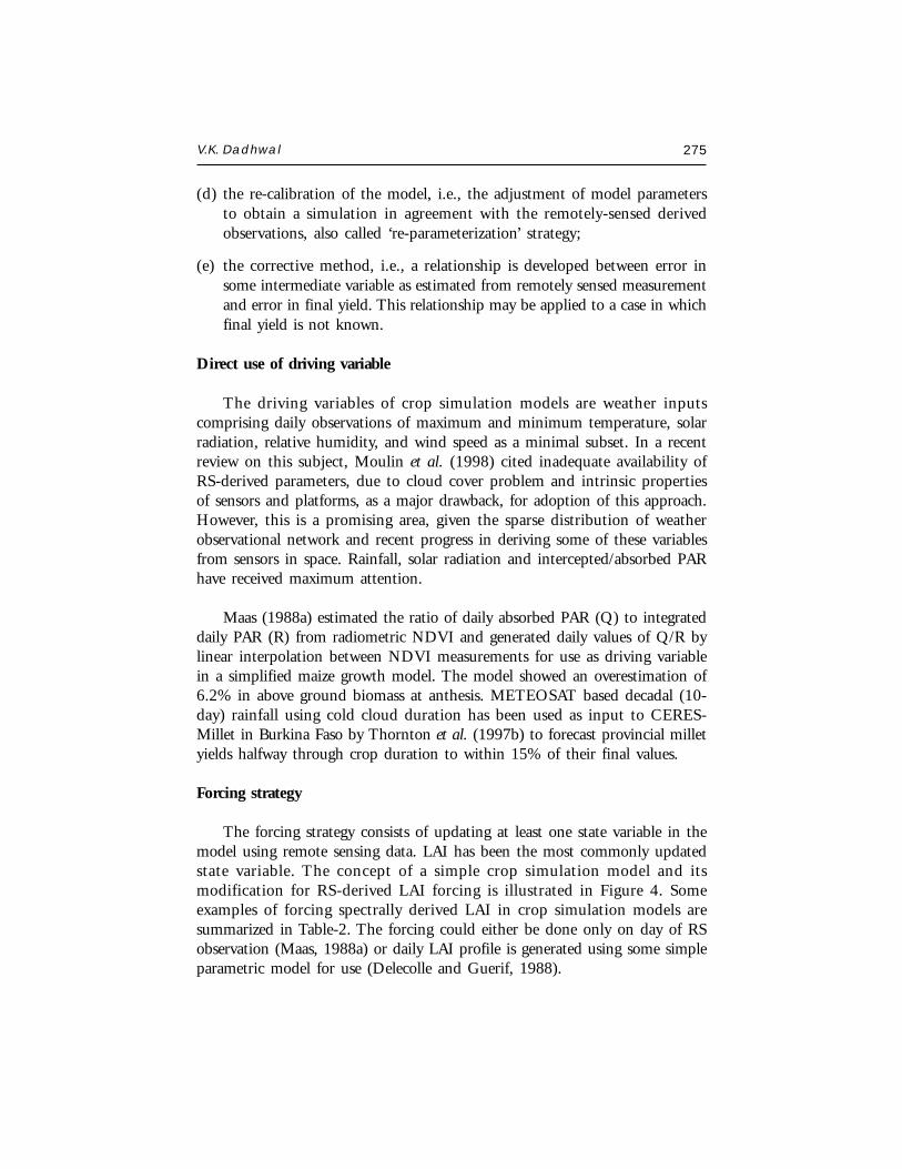
V.K. Dadhwal 275
(d) the re-calibration of the model, i.e., the adjustment of model parametersto obtain a simulation in agreement with the remotely-sensed derivedobservations, also called ‘re-parameterization’ strategy;
(e) the corrective method, i.e., a relationship is developed between error insome intermediate variable as estimated from remotely sensed measurementand error in final yield. This relationship may be applied to a case in whichfinal yield is not known.
Direct use of driving variable
The driving variables of crop simulation models are weather inputscomprising daily observations of maximum and minimum temperature, solarradiation, relative humidity, and wind speed as a minimal subset. In a recentreview on this subject, Moulin et al. (1998) cited inadequate availability ofRS-derived parameters, due to cloud cover problem and intrinsic propertiesof sensors and platforms, as a major drawback, for adoption of this approach.However, this is a promising area, given the sparse distribution of weatherobservational network and recent progress in deriving some of these variablesfrom sensors in space. Rainfall, solar radiation and intercepted/absorbed PARhave received maximum attention.
Maas (1988a) estimated the ratio of daily absorbed PAR (Q) to integrateddaily PAR (R) from radiometric NDVI and generated daily values of Q/R bylinear interpolation between NDVI measurements for use as driving variablein a simplified maize growth model. The model showed an overestimation of6.2% in above ground biomass at anthesis. METEOSAT based decadal (10-day) rainfall using cold cloud duration has been used as input to CERES-Millet in Burkina Faso by Thornton et al. (1997b) to forecast provincial milletyields halfway through crop duration to within 15% of their final values.
Forcing strategy
The forcing strategy consists of updating at least one state variable in themodel using remote sensing data. LAI has been the most commonly updatedstate variable. The concept of a simple crop simulation model and itsmodification for RS-derived LAI forcing is illustrated in Figure 4. Someexamples of forcing spectrally derived LAI in crop simulation models aresummarized in Table-2. The forcing could either be done only on day of RSobservation (Maas, 1988a) or daily LAI profile is generated using some simpleparametric model for use (Delecolle and Guerif, 1988).
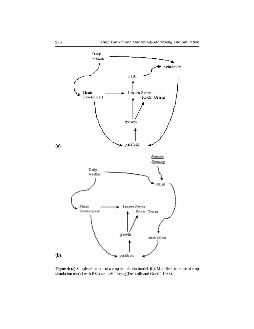
276 Crop Growth and Productivity Monitoring and Simulation
Figure 4: (a) Simple schematic of a crop simulation model. (b). Modified structure of cropsimulation model with RS-based LAI forcing (Delecolle and Guerif, 1988)
(a)
(b)
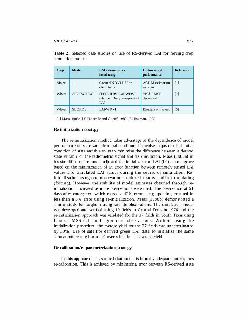
V.K. Dadhwal 277
Table 2. Selected case studies on use of RS-derived LAI for forcing cropsimulation models
Crop Model LAI estimation & Evaluation of Referenceinterfacing performance
Maize - Ground NDVI-LAI on AGDM estimation [1]obs. Dates improved
Wheat AFRCWHEAT SPOT/HRV LAI-WDVI Yield RMSE [2]relation: Daily interpolated decreasedLAI
Wheat SUCROS LAI-WDVI Biomass at harvest [3]
[1] Maas, 1988a; [2] Delecolle and Guerif, 1988; [3] Bouman, 1995
Re-initialization strategy
The re-initialization method takes advantage of the dependence of modelperformance on state variable initial condition. It involves adjustment of initialcondition of state variable so as to minimize the difference between a derivedstate variable or the radiometric signal and its simulation. Maas (1988a) inhis simplified maize model adjusted the initial value of LAI (L0) at emergencebased on the minimization of an error function between remotely sensed LAIvalues and simulated LAI values during the course of simulation. Re-initialization using one observation produced results similar to updating(forcing). However, the stability of model estimates obtained through re-initialization increased as more observations were used. The observation at 51days after emergence, which caused a 42% error using updating, resulted inless than a 3% error using re-initialization. Maas (1988b) demonstrated asimilar study for sorghum using satellite observations. The simulation modelwas developed and verified using 10 fields in Central Texas in 1976 and there-initialization approach was validated for the 37 fields in South Texas usingLandsat MSS data and agronomic observations. Without using theinitialization procedure, the average yield for the 37 fields was underestimatedby 30%. Use of satellite derived green LAI data to initialize the samesimulations resulted in a 2% overestimation of average yield.
Re-calibration/re-parameterization strategy
In this approach it is assumed that model is formally adequate but requiresre-calibration. This is achieved by minimizing error between RS-derived state
278 Crop Growth and Productivity Monitoring and Simulation
variable and its simulation by the model. This makes such an approachsensitive to errors in deriving state variables from RS data. In this case also,the state variable matched is LAI. However, depending on the model structure,which parameter to tune and number of observations used in analysis is critical.
Maas (1988a) demonstrated the re-calibration for maize model withremotely sensed GLAI observations. A multi-dimensional error functionminimization procedure was used which indicated more consistent estimatesof LAI and biomass at anthesis as the number of parameters increased in multi-dimensional re-parameterization.
Delecolle et al. (1992) illustrated the use of re-calibration for rice cropusing GRAMI model. Values of one to four parameters in the GRAMI modelwere re-calibrated to match the simulated LAI profile to observed LAI values.The results showed that improvement in simulated LAI profile by re-calibrationdepends largely on the number and timing of LAI observations. Clevers andLeeuwen (1996) used ground and airborne radiometric measurements oversugar beet fields to calibrate the SUCROS model. They derived LAI frommeasurements in optical and microwave wavebands. The adjusted parametersand initial conditions were sowing date, a growth rate, light use efficiencyand maximum leaf area. The results showed that re-calibration with bothoptical and microwave observations estimated yield better than optical dataalone. In the absence of optical remote sensing data, radar data yielded asignificant improvement in yield estimation with the case of no remotelyobserved observations. Inoue et al. (1998) related paddy vegetation indices tothe fraction of absorbed photosynthetically active radiation (fAPAR) asexponential equations with different parameters for the periods before and afterheading. A real time recalibration module based on a simplex algorithm wasdeveloped and proved effective in linking remotely sensed fAPAR with a simplerice growth model.
Re-parameterization using Coupled Crop Simulation Models and Canopy-radiation Models
The re-initialization and re-parameterization of crop models can also makedirect use of radiometric information instead of deriving canopy parametersfrom them (Moulin et al., 1998). In this strategy, coupling a radiative transferreflectance model to the crop production model reproduces the temporalbehaviour of canopy surface reflectance, which can be compared with canopyreflectance observed from satellite. Adjusting initial conditions or model
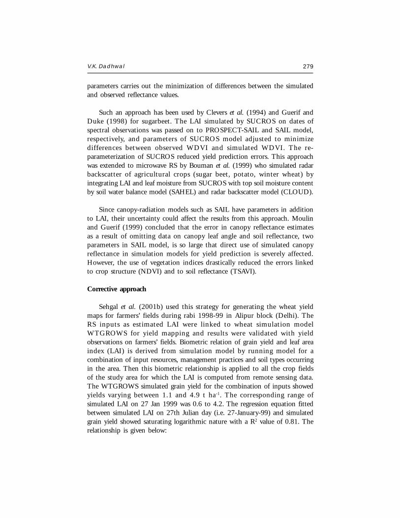
V.K. Dadhwal 279
parameters carries out the minimization of differences between the simulatedand observed reflectance values.
Such an approach has been used by Clevers et al. (1994) and Guerif andDuke (1998) for sugarbeet. The LAI simulated by SUCROS on dates ofspectral observations was passed on to PROSPECT-SAIL and SAIL model,respectively, and parameters of SUCROS model adjusted to minimizedifferences between observed WDVI and simulated WDVI. The re-parameterization of SUCROS reduced yield prediction errors. This approachwas extended to microwave RS by Bouman et al. (1999) who simulated radarbackscatter of agricultural crops (sugar beet, potato, winter wheat) byintegrating LAI and leaf moisture from SUCROS with top soil moisture contentby soil water balance model (SAHEL) and radar backscatter model (CLOUD).
Since canopy-radiation models such as SAIL have parameters in additionto LAI, their uncertainty could affect the results from this approach. Moulinand Guerif (1999) concluded that the error in canopy reflectance estimatesas a result of omitting data on canopy leaf angle and soil reflectance, twoparameters in SAIL model, is so large that direct use of simulated canopyreflectance in simulation models for yield prediction is severely affected.However, the use of vegetation indices drastically reduced the errors linkedto crop structure (NDVI) and to soil reflectance (TSAVI).
Corrective approach
Sehgal et al. (2001b) used this strategy for generating the wheat yieldmaps for farmers’ fields during rabi 1998-99 in Alipur block (Delhi). TheRS inputs as estimated LAI were linked to wheat simulation modelWTGROWS for yield mapping and results were validated with yieldobservations on farmers’ fields. Biometric relation of grain yield and leaf areaindex (LAI) is derived from simulation model by running model for acombination of input resources, management practices and soil types occurringin the area. Then this biometric relationship is applied to all the crop fieldsof the study area for which the LAI is computed from remote sensing data.The WTGROWS simulated grain yield for the combination of inputs showedyields varying between 1.1 and 4.9 t ha-1. The corresponding range ofsimulated LAI on 27 Jan 1999 was 0.6 to 4.2. The regression equation fittedbetween simulated LAI on 27th Julian day (i.e. 27-January-99) and simulatedgrain yield showed saturating logarithmic nature with a R2 value of 0.81. Therelationship is given below:
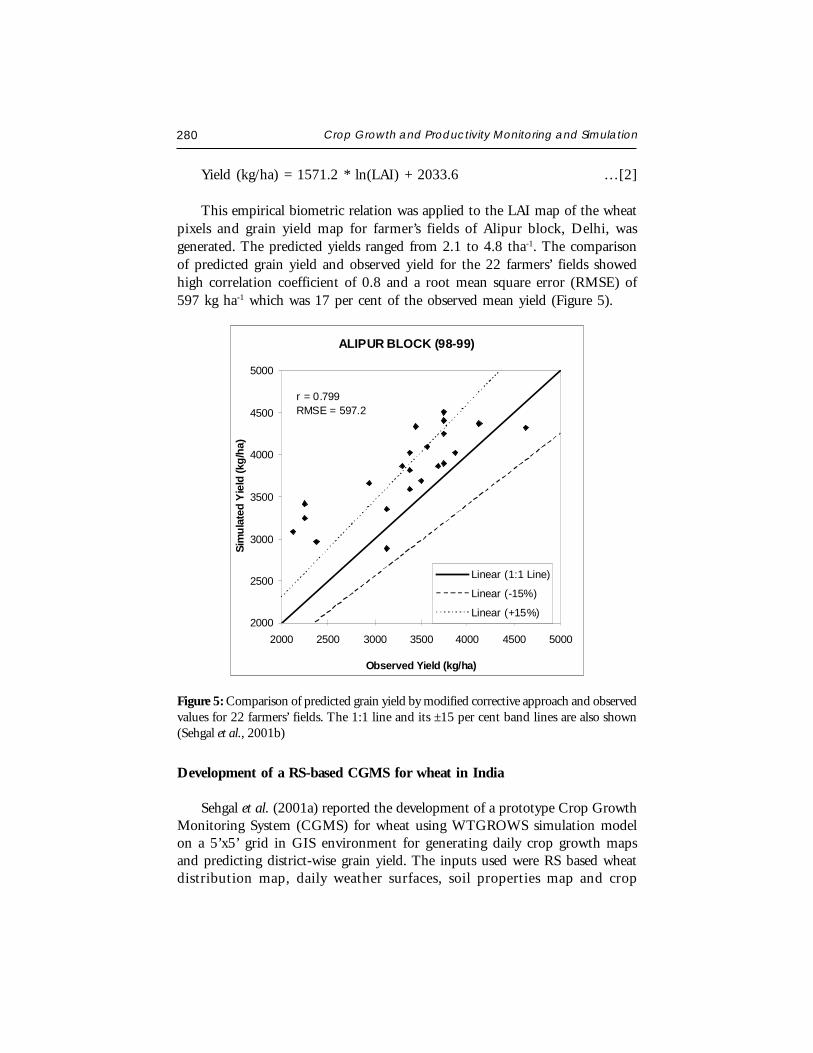
280 Crop Growth and Productivity Monitoring and Simulation
Yield (kg/ha) = 1571.2 * ln(LAI) + 2033.6 …[2]
This empirical biometric relation was applied to the LAI map of the wheatpixels and grain yield map for farmer’s fields of Alipur block, Delhi, wasgenerated. The predicted yields ranged from 2.1 to 4.8 tha-1. The comparisonof predicted grain yield and observed yield for the 22 farmers’ fields showedhigh correlation coefficient of 0.8 and a root mean square error (RMSE) of597 kg ha-1 which was 17 per cent of the observed mean yield (Figure 5).
ALIPUR BLOCK (98-99)
2000
2500
3000
3500
4000
4500
5000
2000 2500 3000 3500 4000 4500 5000
Observed Yield (kg/ha)
Sim
ulat
ed Y
ield
(kg/
ha)
Linear (1:1 Line)
Linear (-15%)
Linear (+15%)
r = 0.799RMSE = 597.2
Figure 5: Comparison of predicted grain yield by modified corrective approach and observedvalues for 22 farmers’ fields. The 1:1 line and its ±15 per cent band lines are also shown(Sehgal et al., 2001b)
Development of a RS-based CGMS for wheat in India
Sehgal et al. (2001a) reported the development of a prototype Crop GrowthMonitoring System (CGMS) for wheat using WTGROWS simulation modelon a 5’x5’ grid in GIS environment for generating daily crop growth mapsand predicting district-wise grain yield. The inputs used were RS based wheatdistribution map, daily weather surfaces, soil properties map and crop
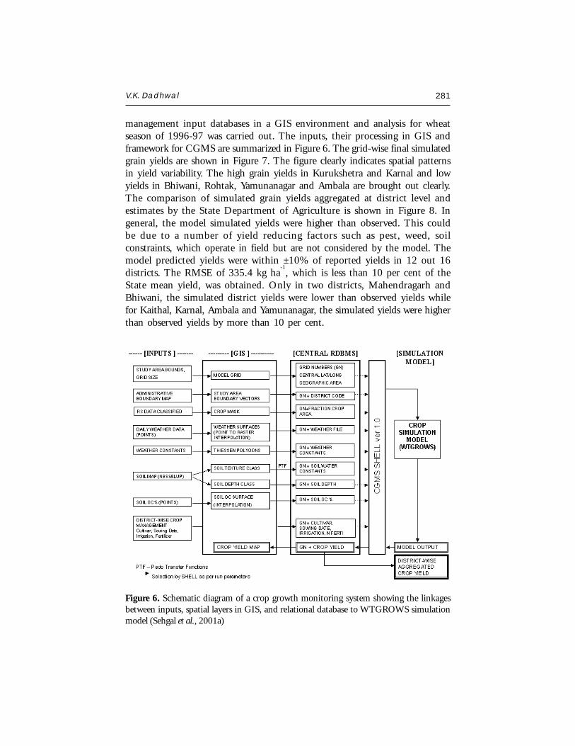
V.K. Dadhwal 281
management input databases in a GIS environment and analysis for wheatseason of 1996-97 was carried out. The inputs, their processing in GIS andframework for CGMS are summarized in Figure 6. The grid-wise final simulatedgrain yields are shown in Figure 7. The figure clearly indicates spatial patternsin yield variability. The high grain yields in Kurukshetra and Karnal and lowyields in Bhiwani, Rohtak, Yamunanagar and Ambala are brought out clearly.The comparison of simulated grain yields aggregated at district level andestimates by the State Department of Agriculture is shown in Figure 8. Ingeneral, the model simulated yields were higher than observed. This couldbe due to a number of yield reducing factors such as pest, weed, soilconstraints, which operate in field but are not considered by the model. Themodel predicted yields were within ±10% of reported yields in 12 out 16districts. The RMSE of 335.4 kg ha
-1, which is less than 10 per cent of the
State mean yield, was obtained. Only in two districts, Mahendragarh andBhiwani, the simulated district yields were lower than observed yields whilefor Kaithal, Karnal, Ambala and Yamunanagar, the simulated yields were higherthan observed yields by more than 10 per cent.
Figure 6. Schematic diagram of a crop growth monitoring system showing the linkagesbetween inputs, spatial layers in GIS, and relational database to WTGROWS simulationmodel (Sehgal et al., 2001a)
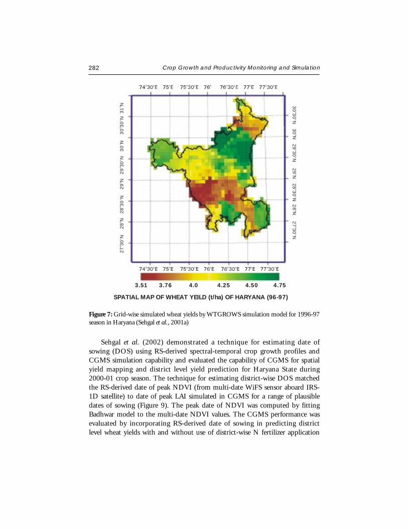
282 Crop Growth and Productivity Monitoring and Simulation
Sehgal et al. (2002) demonstrated a technique for estimating date ofsowing (DOS) using RS-derived spectral-temporal crop growth profiles andCGMS simulation capability and evaluated the capability of CGMS for spatialyield mapping and district level yield prediction for Haryana State during2000-01 crop season. The technique for estimating district-wise DOS matchedthe RS-derived date of peak NDVI (from multi-date WiFS sensor aboard IRS-1D satellite) to date of peak LAI simulated in CGMS for a range of plausibledates of sowing (Figure 9). The peak date of NDVI was computed by fittingBadhwar model to the multi-date NDVI values. The CGMS performance wasevaluated by incorporating RS-derived date of sowing in predicting districtlevel wheat yields with and without use of district-wise N fertilizer application
Figure 7: Grid-wise simulated wheat yields by WTGROWS simulation model for 1996-97season in Haryana (Sehgal et al., 2001a)
27
30’N
28
N 2
830’N
29
N 2
930’N
3
0’N
30
30’N
31
No
oo
oo
oo 3
030’N
30
N 2
930’N
29
N 2
830’N
28
N 2
730’N
oo
oo
oo
o
3.51 3.76 4.0 4.25 4.50 4.75
SPATIAL MAP OF WHEAT YEILD (t/ha) OF HARYANA (96-97)
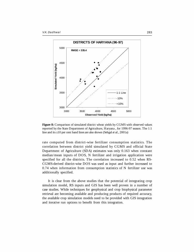
V.K. Dadhwal 283
rate computed from district-wise fertilizer consumption statistics. Thecorrelation between district yield simulated by CGMS and official StateDepartment of Agriculture (SDA) estimates was only 0.163 when constantmedian/mean inputs of DOS, N fertilizer and irrigation application werespecified for all the districts. The correlation increased to 0.52 when RS-CGMS-derived district-wise DOS was used as input and further increased to0.74 when information from consumption statistics of N fertilizer use wasadditionally specified.
It is clear from the above studies that the potential of integrating cropsimulation model, RS inputs and GIS has been well proven in a number ofcase studies. While techniques for geophysical and crop biophysical parameterretrieval are becoming available and producing products of required accuracy,the available crop simulation models need to be provided with GIS integrationand iterative run options to benefit from this integration.
3000
3500
4000
4500
5000
3000 3500 4000 4500 5000Observed Yield (kg/ha)
Sim
ulat
ed Y
ield
(kg/
ha)
1:1 Line
-10%
+10%
RMSE = 335.4
DISTRICTS OF HARYANA (96-97)
Figure 8: Comparison of simulated district wheat yields by CGMS with observed valuesreported by the State Department of Agriculture, Haryana , for 1996-97 season. The 1:1line and its ±10 per cent band lines are also shown (Sehgal et al., 2001a)
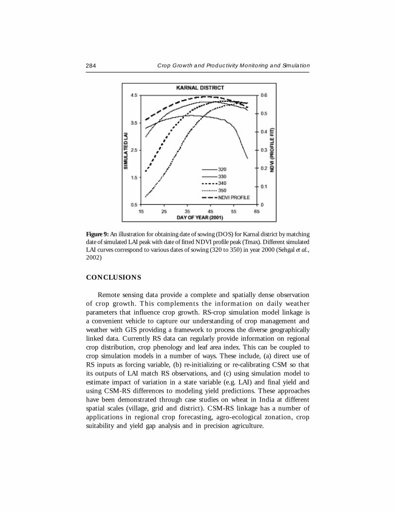
284 Crop Growth and Productivity Monitoring and Simulation
CONCLUSIONS
Remote sensing data provide a complete and spatially dense observationof crop growth. This complements the information on daily weatherparameters that influence crop growth. RS-crop simulation model linkage isa convenient vehicle to capture our understanding of crop management andweather with GIS providing a framework to process the diverse geographicallylinked data. Currently RS data can regularly provide information on regionalcrop distribution, crop phenology and leaf area index. This can be coupled tocrop simulation models in a number of ways. These include, (a) direct use ofRS inputs as forcing variable, (b) re-initializing or re-calibrating CSM so thatits outputs of LAI match RS observations, and (c) using simulation model toestimate impact of variation in a state variable (e.g. LAI) and final yield andusing CSM-RS differences to modeling yield predictions. These approacheshave been demonstrated through case studies on wheat in India at differentspatial scales (village, grid and district). CSM-RS linkage has a number ofapplications in regional crop forecasting, agro-ecological zonation, cropsuitability and yield gap analysis and in precision agriculture.
Figure 9: An illustration for obtaining date of sowing (DOS) for Karnal district by matchingdate of simulated LAI peak with date of fitted NDVI profile peak (Tmax). Different simulatedLAI curves correspond to various dates of sowing (320 to 350) in year 2000 (Sehgal et al.,2002)
V.K. Dadhwal 285
In future the RS-CSM linkage will be broadened due to improvementsin sensor capabilities (spatial resolution, hyper-spectral data) as well as retrievalof additional crop parameters like chlorophyll, leaf N and canopy water status.Thermal remote sensing can provide canopy temperatures and microwave data,the soil moisture. The improved characterization of crop and its growingenvironment would provide additional ways to modulate crop simulationtowards capturing the spatial and temporal dimensions of crop growthvariability.
REFERENCES
Aggarwal, P.K. 1993. Agro-ecological zoning using crop growth simulation models:characterization of wheat environments of India, pages 97-109. In: Systems Approachesfor Agricultural Development, Vol. 2. (Penning de Vries, F.W.T., Teng, P. and Metselaar,K. eds.), Kluwer Academic Publishers, Dordrecht, The Netherlands.
Aggarwal, P.K., Kalra, N., Bandhyopadhyay, S.K., Pathak, H., Sehgal, V.K., Kaur, R., Rajput,T.B.S., Joshi, H.C., Choudhary, R. and Roetter, R. 1998. Exploring agricultural landuse options for the State of Haryana: Biophysical modelling, pages 59-65. In: Exchangeof methodologies in land use planning (Roetter, R., Hoanh, C.T., Luat, N.V., vanlttersum, M.K. and van Laar, H.H. eds.), SysNet Research Paper Series No. 1, IRRI, LosBanos, Philippines.
Bacsi, Z., Thorton, P.K. and Dent, J.B. 1991. Impacts of future climate change on Hungariancrop production: An application of crop growth simulation models. Agric. Sys., 37:435-450.
Badhwar, G. D., MacDonald, R.B., and Mehta, N.C. 1986. Satellite-derived LAI andvegetation maps as input to global cycle models-a hierarchical approach. Int. J. RemoteSensing, 7: 265-281.
Bouman, B.A.M. 1995. Crop modelling and remote sensing for yield prediction. NetherlandJ. Agric. Sci., 43: 143-161.
Bouman, B.A.M., van Dipen, C.A., Vossen, P. and van Der Wal, T. 1997. Simulation andsystems analysis tools for crop yield forecasting, pages 325-340. In: Applications ofSystems Approaches at the Farm and Regional Levels, Vol. 1. (Teng, P.S., Kropff, M.J.,ten Berge, H.F.M., Dent, J.B., Lansigan, F.P. and van Laar, H.H. eds.), Kluwer AcademicPublishers, Dordrecht, The Netherlands.
Bouman, B.A.M., van Kraalingen, D.W.G., Stol, W. and van Leeuwen, H.J.C. 1999. Anecological modeling approach to explain ERS SAR radar backscatter of agricultural crops.Remote Sens. Environ., 67: 137-146.
286 Crop Growth and Productivity Monitoring and Simulation
Burrough, P.A. and McDonnell, R.A. 1998. Principles of geographic information systems.Oxford University Press, Oxford, UK, pp. 10-16.
Burrough, P.A. 1996. Environmental modelling with geographical information system, pages56-59. In: Models in Action, Quantitative Approaches in Systems Analysis (Stein, A.,Penning de Vries, F.W.T. and Schotman, P.J. eds.), No 6, AB-DLO, Wageningen, TheNetherlands.
Calixte, J.P., Beinroth, F.J., Jones, J.W. and Lai, H. 1992. Linking DSSAT to a geographicinformation system. Agrotechnology Transfer, 15: 1-7.
Carter, T.R. and Saariko, R.A. 1996. Estimating regional crop potential in Finland under achanging climate. Agric. For. Meteorol., 79: 301-313.
Chen, J.M. and Cihlar, J. 1996. Retrieving leaf area index of boreal conifer forests usingLandsat TM images. Remote Sens.Environ., 55: 153-162.
Chen, J.M., Pavlic, G., Brown, L., Cihlar, J., Leblanc, S.G., White, H.P., Hall, R.J., Peddle,D.R., King, D.J., Trofymow, J.A., Swift, E., Van der Sanden, J., Pellikka, P.K.E. 2002.Derivation and validation of Canada-wide coarse-resolution leaf area index maps usinghigh-resolution satellite imagery and ground measurements. Remote Sens. Environ., 80:165-184.
Clevers, J.G.P.W., Buker, C., van Leeuwen, H.J.C. and Bouman, B.A.M. 1994. A frameworkfor monitoring crop growth by combining directional and spectral remote sensinginformation. Remote Sens. Environ., 50: 161-170.
Clevers, J.G.P.W. and van Leeuwen, H.J.C. 1996. Combined use of optical and microwaveremote sensing data for crop growth monitoring. Remote Sens. Environ., 56: 42 - 51.
Dadhwal, V.K. 1999. Remote Sensing and GIS for agricultural crop acreage and yieldestimation. Internat. Arch. Photogramm. & Remote Sensing, XXXII, 7-W9, 58-67.
Dadhwal, V.K. and Ray, S.S. 2000. Crop Assessment using remote sensing – Part II: Cropcondition and yield assessment. Indian J. Agric. Economics, 55 (2, Suppl.), 55-67.
Dadhwal, V.K., Sehgal, V.K., Singh, R.P. and Rajak, D.R. 2003. Wheat yield modeling usingsatellite remote sensing with weather data: Recent Indian experience. Mausum, 54(1):253-262.
Delecolle, R. and Guerif, M. 1988. Introducing spectral data into a plant process model forimproving its prediction ability. Proceedings of the 4th International ColloquiumSignatures Spectrales d’Objects en Teledetection, 18-22 Jan, 1988, Aussois, France, pp.125-127.
V.K. Dadhwal 287
Delecolle, R., Maas, S.J., Guerif., M. and Baret, F. 1992. Remote sensing and crop productionmodels: present trends. ISPRS J. Photogramm. Remote Sens., 47:145-161.
Engel, T., Hoogenboom, G., Jones, J.W. and Wilkens, P.W. 1997. AEGIS/WIN - a programfor the application of crop simulation models across geographic areas. Agronomy J., 89:919-928.
Gao, W. and Lesht, B.M. 1997. Model inversion of satellite measured reflectances to obtainsurface biophysical and bi-directional reflectance characteristics of grassland. Remote Sens.Environ., 59: 461-471.
Guerif, M. and Duke, C. 1998. Calibration of SUCROS emergence and early growth modulefor sugar beet using optical remote sensing data assimilation. European J. Agronomy, 9:127-136.
Han, S., Evans, R.G., Hodges, T. and Rawlins, S.L. 1995. Linking geographic informationsystem with a potato simulation model for site-specific crop management. J. Environ.Qual., 24: 772-777.
Hartkamp, D.A., White, J.W. and Hoogenboom, G. 1999. Interfacing geographicinformation systems with agronomic modeling: A review. Agron. J., 91: 761-772.
Horie, T., Yajima, M. and Nakagawa, H. 1992. Yield forecasting. Agric. For. Meteorol., 40:211-236.
Inoue, Y., Moran, M.S. and Horie, T. 1998. Analysis of spectral measurements in paddyfield for predicting rice growth and yield based on a simple crop simulation model.Plant Production Sci., 1(4): 269-279.
Jones, J.W. 1993. Decision support systems for agricultural development, pages 459-471.In: Systems Approaches for Agricultural Development, Vol. 2. (Penning de Vries, F.W.T.,Teng, P. and Metselaar, K. eds.), Kluwer Academic Publishers, Dordrecht, TheNetherlands.
Knyazikhin, Y., Martonchik, J.V., Myneni, R.B., Diner, D.J. and Running, S.W. 1998.Synergistic algorithm for estimating vegetation canopy leaf area index and fraction ofabsorbed photosynthetically active radiation from MODIS and MISR data. J. Geophys.Res., 103: 32257-32275.
Maas, S.J. 1988a. Use of remotely sensed information in agricultural crop growth models.Ecol. Modelling, 41: 247-268.
Maas, S.J. 1988b. Using satellite data to improve model estimates of crop yield. Agron. J.,80: 655-662.
288 Crop Growth and Productivity Monitoring and Simulation
Maracchi, G., Perarnaud, V. and Kleschenko, A.D. 2000. Applications of geographicalinformation systems and remote sensing in agrometeorology. Agric. Forest Meteorol., 103:119-136.
Meyer-Roux, J. and Vossen, P. 1994. The first phase of the MARS project, 1988-1993:overview, methods and results, pp. 33 – 85. In: Proceedings of the Conference on theMARS Project: Overview and Perspectives. Commission of the European Communities,Luxembourg.
Moulin, S. and Guerif, M. 1999. Impacts of model parameter uncertainties on crop reflectanceestimates: a regional case study on wheat. Int. J. Remote Sens., 20(1): 213-218.
Moulin, S., Bondeau, A. and Delecolle, R. 1998. Combining agricultural crop models andsatellite observations: from field to regional scales. Int. J. Remote Sens., 19(6): 1021-1036.
Myneni, R.B., Nemani, R.R. and Running, S.W. 1997. Estimation of global leaf area indexand absorbed PAR using radiative transfer models. IEEE Trans. on Geosc. and Rem.Sensing, 35(6): 1380-1393.
Nain, A.S., Dadhwal, V.K. and Singh, T.P. 2004. Use of CERES-Wheat model for wheatyield forecast in central Indo-Gangetic plains of India. J. Agricultural Science (camb.),142: 59-70.
Pandya, M.R., Chaudhari, K.N., Singh, R.P., Sehgal, V.K., Bairagi, G.D., Sharma, R. andDadhwal, V.K. 2003. Leaf area index retrieval using IRS LISS-III sensor data andvalidation of MODIS LAI product over Madhya Pradesh. Current Science, 85(12):1777-1782.
Price, J.C. 1993. Estimating leaf area index from satellite data. IEEE Trans. Geoscience RemoteSensing, 31: 727-734.
Qiu, J., Gao, W. and Lesht, B.M. 1998. Inverting optical reflectance to estimate surfaceproperties of vegetation canopies. Int. J. Remote Sens., 19: 641-656.
Rastogi, A., Kalra, N., Agarwal, P.K., Sharma, S.K., Harit, R.C., Navalgund, R.R. andDadhwal, V.K. 2000. Estimation of wheat leaf area index from satellite data using Pricemodel. International J. Remote Sensing, 21(15): 2943- 2949.
Richardson, A.J., Wiegand, C.L., Arkin, G.F., Nixon, P.R. and Gerbermann, A.H. 1982.Remotely sensed spectral indicators of sorghum development and their use in growthmodelling. Agric. Meteorol., 26: 11-23.
Satya, P., Shibasaki, R. and Ochi, S. 1998. Modelling Spatial Crop Production: A GISapproach. In: Proceedings of the 19th Asian Conference on Remote Sensing, 16-20Nov., 1998, Manila, pp. A-9-1 – A-9-6.
V.K. Dadhwal 289
Sehgal, V.K., Rajak, D.R. and Dadhwal, V.K. 2001a. Issues in linking remote sensing inputsin a crop growth monitoring system: results of a case study. In: Proc. of the ISRS NationalSymposium, Dec 11-13, 2001, Ahmedabad, India.
Sehgal, V.K., Sastri, C.V.S., Kalra, N. and Dadhwal, V.K. 2001b. Farm level yield mappingfor precision crop management under Indian conditions using a simple approach oflinking remote sensing information and crop simulation model. In: Proc. of the ISRSNational Symposium, Dec 11-13, 2001, Ahmedabad, India.
Sehgal, V.K., Rajak, D.R., Chaudhary, K.N. and Dadhwal, V.K. 2002. Improved regionalyield prediction by crop growth monitoring system using remote sensing derived cropphenology. Internat. Arch. Photogramm. Remote Sens. & Spatial Inf. Sci., 34 (7): 329-334.
Thornton, P.K., Bowen, W.T., Ravelo, A.C., Wilkens, P.W., Farmer, G., Brock, J. and Brink,J.E. 1997. Estimating millet production for famine early warning: an application ofcrop simulation modelling using satellite and ground-based data in Burkina Faso. Agric.For. Meteorol, 83: 95-112.
Tim, U.S. 1996. Coupling vadose zone models with GIS: Emerging trends and potentialbottlenecks. J. Environ. Qual., 25: 535-544.
Vossen, P. 1995. Early assessment of national yields: the approach developed by the MARS-STAT project on behalf of European Commission, pages 327-347. In: Proceedings ofthe Seminar on Yield Forecasting, 24-27 Oct., 1995, Villerfranche-sur-Mer, France.
Wade, G., Mueller, R., Cook, P.W. and Doraiswamy, P.C. 1994. AVHRR Map products forCrop Condition Assessment: A Geographic Information Systems Approach.Photogrammetric Engineering & Remote Sensing, 60(9): 1145-1150.
Wiegand, C.L., Richardsons, A.J. and Kanemasu, E.T. 1979. Leaf area index estimates forwheat from LANDSAT and their implications for evapotranspiration and crop modeling.Agronomy J., 71: 336-342.
DROUGHTS & FLOODS ASSESSMENT ANDMONITORING USING REMOTE SENSINGAND GIS
A.T. Jeyaseelan
Crop Inventory and Drought Assessment DivisionNational Remote Sensing AgencyDepartment of Space, Govt. of India, Hyderabad
Abstract : Space technology has made substantial contribution in all the three phasessuch as preparedness, prevention and relief phases of drought and flood disastermanagement. The Earth Observation satellites which include both geostationary andpolar orbiting satellites provide comprehensive, synoptic and multi temporal coverageof large areas in real time and at frequent intervals and ‘thus’ - have become valuablefor continuous monitoring of atmospheric as well as surface parameters related todroughts and floods. Geo-stationary satellites provide continuous and synopticobservations over large areas on weather including cyclone monitoring. Polar orbitingsatellites have the advantage of providing much higher resolution imageries, eventhough at low temporal frequency, which could be used for detailed monitoring,damage assessment and long-term relief management. Advancements in the remotesensing technology and the Geographic Information Systems help in real timemonitoring, early warning and quick damage assessment of both drought and flooddisasters. In this lecture the use of remote sensing and GIS and the global scenario for
the drought and flood disaster management is discussed.
INTRODUCTION
Droughts and floods are water-related natural disasters which affect a widerange of environmental factors and activities related to agriculture, vegetation,human and wild life and local economies. Drought is the single most importantweather-related natural disaster often aggravated by human action, since itaffects very large areas for months and years and thus has a serious impact onregional food production, life expectancy for entire populations and economicperformance of large regions or several countries. During 1967-1991, droughts
Satellite Remote Sensing and GIS Applications in Agricultural Meteorologypp. 291-313
292 Droughts & Floods Assessment and Monitoring
have affected 50 per cent of the 2.8 billion people who suffered from all naturaldisasters and killed 35 per cent of the 3.5 million people who lost their lives.In the recent years large-scale intensive droughts have been observed in allcontinents leading to huge economic losses, destruction of ecological resources,food shortages and starvation of millions people. Floods are among the mostdevastating natural hazards in the world, claiming more lives and causing moreproperty damage than any other natural phenomena.
Several users such as top level policy makers at the national and internationalorganisations, researchers, middle level policy makers at the state, province andlocal levels consultants, relief agencies and local producers including farmers,suppliers, traders and water managers are interested in reliable and accuratedrought and flood information for effective management. The disastermanagement activities can be grouped into three major phases: The Preparednessphase where activities such as prediction and risk zone identification are takenup long before the event occurs; the Prevention phase where activities such asEarly warning/Forecasting, monitoring and preparation of contingency plansare taken up just before or during the event; and the Response/Mitigationphase where activities are undertaken just after the event which include damageassessment and relief management.
Remote sensing techniques make it possible to obtain and distributeinformation rapidly over large areas by means of sensors operating in severalspectral bands, mounted on aircraft or satellites. A satellite, which orbits theEarth, is able to explore the whole surface in a few days and repeat the survey ofthe same area at regular intervals, whilst an aircraft can give a more detailedanalysis of a smaller area, if a specific need occurs. The spectral bands used bythese sensors cover the whole range between visible and microwaves. Rapiddevelopments in computer technology and the Geographical InformationSystems (GIS) help to process Remote Sensing (RS) observations from satellitesin a spatial format of maps - both individually and along with tabular data and“crunch” them together to provide a new perception - the spatial visualisationof information of natural resources. The integration of information derived fromRS techniques with other datasets - both in spatial and non-spatial formatsprovides tremendous potential for identification, monitoring and assessmentof droughts and floods.
REMOTE SENSING FOR DROUGHTS
Monitoring and assessment of drought through remote sensing and GISdepend on the factors that cause drought and the factors of drought impact.
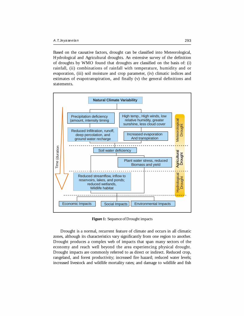
A.T. Jeyaseelan 293
Based on the causative factors, drought can be classified into Meteorological,Hydrological and Agricultural droughts. An extensive survey of the definitionof droughts by WMO found that droughts are classified on the basis of: (i)rainfall, (ii) combinations of rainfall with temperature, humidity and orevaporation, (iii) soil moisture and crop parameter, (iv) climatic indices andestimates of evapotranspiration, and finally (v) the general definitions andstatements.
Figure 1: Sequence of Drought impacts
Drought is a normal, recurrent feature of climate and occurs in all climaticzones, although its characteristics vary significantly from one region to another.Drought produces a complex web of impacts that span many sectors of theeconomy and reach well beyond the area experiencing physical drought.Drought impacts are commonly referred to as direct or indirect. Reduced crop,rangeland, and forest productivity; increased fire hazard; reduced water levels;increased livestock and wildlife mortality rates; and damage to wildlife and fish
Natural Climate Variability
High temp., High winds, low relative humidity, greater
sunshine, less cloud cover
Reduced Infiltration, runoff, deep percolation, and ground water recharge
Increased evaporationAnd transpiration
Soil water deficiency
Plant water stress, reducedBiomass and yield
Reduced streamflow, inflow to reservoirs, lakes, and ponds;
reduced wetlands, Wildlife habitat
Economic Impacts Social Impacts Environmental Impacts
Hyd
rolo
gica
lD
roug
htAg
ricul
tura
lD
roug
htM
eteo
rolo
gica
lD
roug
ht
Precipitation deficiency (amount, intensity timing
Agric
ultu
ral
Dro
ught
T im
e ( d
urat
ion
294 Droughts & Floods Assessment and Monitoring
habitat are a few examples of direct impacts. The consequences of these impactsillustrate indirect impacts. The remote sensing and GIS technology significantlycontributes to all the activities of drought management.
Drought Preparedness Phase
Long before the drought event occurs, the preparedness in terms ofidentifying the drought prone / risk zone area and the prediction of droughtand its intensity is essential.
Drought Prone/Risk zone identification
The drought prone area or risk zone identification is usually carried out onthe basis of historic data analysis of rainfall or rainfall and evaporation and thearea of irrigation support. The conventional methods lack identification of spatialvariation and do not cover man’s influence such as land use changes like irrigatedarea developed and the area affected due to water logging and salinity. Theremote-sensing based method for identification of drought prone areas(Jeyaseelan et al., 2002) uses historical vegetation index data derived from NOAAsatellite series and provides spatial information on drought prone area dependingon the trend in vegetation development, frequency of low development andtheir standard deviations.
Drought prediction
The remote sensing use for drought prediction can benefit from climatevariability predictions using coupled ocean/atmosphere models, survey of snowpacks, persistent anomalous circulation patterns in the ocean and atmosphere,initial soil moisture, assimilation of remotely sensed data into numericalprediction models and amount of water available for irrigation. Nearly-globalseasonal climate anomaly predictions are possible due to the successfulcombination of observational satellite networks for operational meteorological,oceanographic and hydrological observations. Improved coupled models andnear-real time evaluation of in situ and remote sensing data - allows for the firsttime physically-based drought warnings several months in advance, to which agrowing number of countries already relate their policies in agriculture, fisheriesand distribution of goods.
The quality of seasonal predictions of temperature and precipitationanomalies by various centres such as the National Climate Research Centre
A.T. Jeyaseelan 295
(NCRC) of United States, the European Centre for Medium Range WeatherForecasts (ECMWF), the India Meteorological Department (IMD), the NationalCentre for Medium Range Weather Forecast of India (NCMRWF) is a functionof the quality and amount of satellite data assimilated into the starting fields(e.g., SST from AVHRR and profiles from TOVS on NOAA satellites, ERS-2scatterometer winds, SSM/I on DMSP satellites and all geostationary weathersatellites: Geostationary Operational Environmental Satellites (GOES), i.e.GOES-East, GOES-West of USA, METeorological SATellite (METEOSAT) ofEurope, Geostationary Meteorological Satellites (GMS) of Japan, IndianNational Satellites (INSAT) of India etc.). The new assimilation techniqueshave produced a stronger impact of space data on the quality of weather andseasonal climate predictions.
The potential contribution by existing satellites is by far not fully exploited,since neither the synergy gained by the combination of satellite sensors is usednor all the satellite data are distributed internationally. For example, betterinformation flow is needed from satellite data producers to the intermediaryservices such as CLIPS (Climate Information and Prediction Services) projectof World Meteorological Organisation (WMO), and prediction centres includingthe European Centre for Medium Range Weather Forecasts (ECMWF), NationalCentres for Environmental Predictions (NCEP), Japan Meteorological Agency(JMA), India Meteorological Department (IMD), National Centre for MediumRange Weather Forecast, India (NCMRWF) etc. to local services and ultimatelyto end users. Further the drought predictions need to be improved with ElNiño predictions and should be brought down to larger scales.
Drought Prevention Phase
Drought Monitoring and Early Warning
Drought monitoring mechanism exists in most of the countries based onground based information on drought related parameters such as rainfall,weather, crop condition and water availability, etc. Earth observations fromsatellite are highly complementary to those collected by in-situ systems. Satellitesare often necessary for the provision of synoptic, wide-area coverage and frequentinformation required for spatial monitoring of drought conditions. The presentstate of remotely sensed data for drought monitoring and early warning is basedon rainfall, surface wetness, temperature and vegetation monitoring.

296 Droughts & Floods Assessment and Monitoring
Currently, multi channel and multi sensor data sources from geostationaryplatforms such as GOES, METEOSAT, INSAT and GMS and polar orbitingsatellites such as National Oceanic Atmospheric and Administration (NOAA),EOS-Terra, Defense Meteorological Satellite Program (DMSP) and IndianRemote Sensing Satellites (IRS) have been used or planned to be used formeteorological parameter evaluation, interpretation, validation and integration.These data are used to estimate precipitation intensity, amount, and coverage,and to determine ground effects such as surface (soil) wetness.
Rainfall Monitoring
Rain is the major causative factor for drought. As the conventional methodis based on the point information with limited network of observations, theremote sensing based method provides better spatial estimates. Though thesatellite based rainfall estimation procedure is still experimental, the methodscan be grouped into 3 types namely Visible and Infrared (VIS and IR) technique,passive microwave technique and active microwave technique.
VIS and IR technique: VIS and IR techniques were the first to be conceivedand are rather simple to apply while at the same time they show a relativelylow degree of accuracy. A complete overview of the early work and physicalpremises of VIS and thermal IR (10.5 – 12.5 µm) techniques is provided byBarrett and Martin (1981) and Kidder and Vonder Haar (1995). The Rainfallestimation methods can be divided into the following categories: cloud-indexing,bi-spectral, life history and cloud model. Each of the categories stresses aparticular aspect of cloud physics properties using satellite imagery.
Cloud indexing techniques assign a rain rate level to each cloud typeidentified in the satellite imagery. The simplest and perhaps most widely usedis the one developed by Arkin (1979). A family of cloud indexing algorithmswas developed at the University of Bristol, originally for polar orbiting NOAAsatellites and recently adapted to geostationary satellite imagery. “Rain Days”are identified from the occurrence of IR brightness temperatures (TB) below athreshold.
Bi-spectral methods are based on the very simple, although not alwaystrue, relationship between cold and bright clouds and high probability ofprecipitation, this is characteristic of Cumulonimbus. Lower probabilities areassociated with cold but dull clouds (thin cirrus) or bright but warm (stratus)clouds. O’Sullivan et al. (1990) used brightness and textural characteristics
A.T. Jeyaseelan 297
during daytime and IR temperature patterns to estimate rainfall over a 10 × 10pixel array in three categories: no rain, light rain, and moderate/heavy rain. Afamily of techniques that specifically require geostationary satellite imagery arethe life-history methods that rely upon a detailed analysis of the cloud’s lifecycle, which is particularly relevant for convective clouds. An example is theGriffith-Woodley technique (Griffith et al., 1978). Cloud model techniquesaim at introducing the cloud physics into the retrieval process for a quantitativeimprovement deriving from the overall better physical description of the rainformation processes. Gruber (1973) first introduced a cumulus convectionparameterization to relate fractional cloud cover to rain rate. A one-dimensionalcloud model relates cloud top temperature to rain rate and rain area in theConvective Stratiform Technique (CST) (Adler and Negri, 1988; Anagnostouet al., 1999).
Passive microwave technique: Clouds are opaque in the VIS and IR spectralrange and precipitation is inferred from cloud top structure. At passive MWfrequencies, precipitation particles are the main source of attenuation of theupwelling radiation. MW techniques are thus physically more direct than thosebased on VIS/IR radiation. The emission of radiation from atmospheric particlesresults in an increase of the signal received by the satellite sensor while at thesame time the scattering due to hydrometeors reduce the radiation stream.Type and size of the detected hydrometeors depends upon the frequency of theupwelling radiation. Above 60 GHz ice scattering dominates and the radiometerscan only sense ice while rain is not detected. Below about 22 GHz absorptionis the primary mechanism affecting the transfer of MW radiation and ice abovethe rain layer is virtually transparent. Between 19.3 and 85.5 GHz, frequencyrange radiation interacts with the main types of hydrometeors, water particlesor droplets (liquid or frozen). Scattering and emission happen at the same timewith radiation undergoing multiple transformations within the cloud columnin the sensor’s field of view (FOV). The biggest disadvantage is the poor spatialand temporal resolution, the first due to diffraction, which limits the groundresolution for a given satellite MW antenna, and the latter to the fact that MWsensors are consequently only mounted on polar orbiters. The matter is furthercomplicated by the different radiative characteristics of sea and land surfacesunderneath. The major instruments used for MW-based rainfall estimationsare the SSM/I, a scanning-type instrument that measures MW radiation over a1400-km wide swath at four separate frequencies, 19.35, 22.235, 37.0 and85.5 GHz, the latter extending the spectral range of previous instruments intothe strong scattering regime (as regards to precipitation-size particles).
298 Droughts & Floods Assessment and Monitoring
Active microwave: The most important precipitation measuring instrumentsfrom space is the PR, precipitation radar operating at 13.8 GHz on boardTRMM, the first of its kind to be flown on board a spacecraft. The instrumentaims at providing the vertical distribution of rainfall for the investigation of itsthree-dimensional structure, obtaining quantitative measurements over landand oceans, and improving the overall retrieval accuracy by the combined useof the radar, and the TMI and VIRS instruments.
Surface Temperature Estimation
The estimation of water stress in crop/ vegetation or low rate ofevapotranspiration from crop is another indicator of drought. As water stressincreases the canopy resistance for vapor transport results in canopy temperaturerise in order to dissipate the additional sensible heat. Sensible heat transport(ET) between the canopy (Ts) and the air (Ta) is proportional to the temperaturedifference (Ts-Ta). Therefore the satellite based surface temperature estimationis one of the indicators for drought monitoring since it is related to the energybalance between soil and plants on the one hand and atmosphere and energybalance on the other in which evapotranspiration plays an important role. Surfacetemperature could be quite complementary to vegetation indices derived fromthe combination of optical bands. Water-stress, for example, should be noticedfirst by an increase in the brightness surface temperature and, if it affects theplant canopy, there will be changes in the optical properties.
During the past decade, significant progress has been made in the estimationof land-surface emissivity and temperature from airborne TIR data. Kahle et al.(1980) developed a technique to estimate the surface temperature based on anassumed constant emissivity in one channel and previously determinedatmospheric parameters. This temperature was then used to estimate theemissivity in other channels (Kahle, 1986). Other techniques such as thermallog residuals and alpha residuals have been developed to extract emissivity frommulti-spectral thermal infrared data (Hook et al., 1992). Based on thesetechniques and an empirical relationship between the minimum emissivityand the spectral contrast in band emissivities, a Temperature EmissivitySeparation (TES) method has been recently developed for one of the ASTER(Advance Space borne Thermal Emission and Reflection Radiometer) products(ATBD-AST-03, 1996).
In addition, three types of methods have been developed to estimate LSTfrom space: the single infrared channel method, the split window method which
A.T. Jeyaseelan 299
is used in various multi-channel sea-surface temperature (SST) algorithms, anda new day/night MODIS LST method which is designed to take advantage ofthe unique capability of the MODIS instrument. The first method requiressurface emissivity and an accurate radiative transfer model and atmosphericprofiles which must be given by either satellite soundings or conventionalradiosonde data. The second method makes corrections for the atmosphericand surface emissivity effects with surface emissivity as an input based on thedifferential absorption in a split window. The third method uses day/nightpairs of TIR data in seven MODIS bands for simultaneously retrieving surfacetemperatures and band-averaged emissivities without knowing atmospherictemperature and water vapor profiles to high accuracy. This method improvesupon the Li and Becker’s method (1993), which estimates both land surfaceemissivity and LST by the use of pairs of day/night co-registered AVHRR imagesfrom the concept of the temperature independent spectral index (TISI) inthermal infrared bands and based on assumed knowledge of surface TIR BRDF(Bi-directional Reflectance Distribution Function) and atmospheric profiles.
Because of the difficulties in correcting both atmospheric effects and surfaceemissivity effects, the development of accurate LST algorithms is not easy. Theaccuracy of atmospheric corrections is limited by radiative transfer methodsand uncertainties in atmospheric molecular (especially, water vapor) absorptioncoefficients and aerosol absorption/scattering coefficients and uncertainties inatmospheric profiles as inputs to radiative transfer models. Atmospherictransmittance/radiance codes LOWTRAN6 (Kneizys et al., 1983),LOWTRAN7 (Kneizys et al., 1988), MODTRAN (Berk et al., 1989), andMOSART (Cornette et al., 1994) have been widely used in development ofSST and LST algorithms and the relation between NDVI and emissivities areused.
Soil Moisture Estimation
Soil moisture in the root zone is a key parameter for early warning ofagricultural drought. The significance of soil moisture is its role in thepartitioning of the energy at the ground surface into sensible and latent(evapotranspiration) heat exchange with the atmosphere, and the partitioningof precipitation into infiltration and runoff.
Soil moisture can be estimated from : (i) point measurements, (ii) soilmoisture models and (iii) remote sensing. Traditional techniques for soil moistureestimation/ observation are based on point basis, which do not always represent
300 Droughts & Floods Assessment and Monitoring
the spatial distribution. The alternative has been to estimate the spatialdistribution of soil moisture using a distributed hydrologic model. However,these estimates are generally poor, due to the fact that soil moisture exhibitslarge spatial and temporal variation as a result of inhomogeneities in soilproperties, vegetation and precipitation. Remote sensing can be used to collectspatial data over large areas on routine basis, providing a capability to makefrequent and spatially comprehensive measurements of the near surface soilmoisture. However, problems with these data include satellite repeat time anddepth over which soil moisture estimates are valid, consisting of the top fewcentimetres at most. These upper few centimetres of the soil is the most exposedto the atmosphere, and their soil moisture varies rapidly in response to rainfalland evaporation. Thus to be useful for hydrologic, climatic and agriculturalstudies, such observations of surface soil moisture must be related to the completesoil moisture profile in the unsaturated zone. The problem of relating soilmoisture content at the surface to that of the profile as a whole has been studiedfor the past two decades. The results of the study indicated following fourapproaches : (i) regression, (ii) knowledge based, (iii) inversion and (iv)combinations of remotely sensed data with soil water balance models.
Passive microwave sensing (radiometry) has shown the greatest potentialamong remote sensing methods for the soil moisture measurement.Measurements at 1 to 3 GHz are directly sensitive to changes in surface soilmoisture, are little affected by clouds, and can penetrate moderate amounts ofvegetation. They can also sense moisture in the surface layer to depths of 2 to 5cm (depending on wavelength and soil wetness). With radiometry, the effect ofsoil moisture on the measured signal dominates over that of surface roughness(whereas the converse is true for radar). Higher frequency Earth-imagingmicrowave radiometers, including the Scanning Multichannel MicrowaveRadiometer (lowest frequency 6.6 GHz) launched on the Seasat (1978) andNimbus-7 (1978-87) satellites, and the Special Sensor Microwave Imager (lowestfrequency 19.35 GHz) launched on the DMSP satellite series have been utilizedin soil moisture studies with some limited success. The capabilities of thesehigher frequency instruments are limited to soil moisture measurements overpredominantly bare soil and in a very shallow surface layer (<5 cm). At itslowest frequency of 19.35 GHz the SSM/I is highly sensitive to even smallamounts of vegetation, which obscures the underlying soil. Large variations insoil moisture (e.g., flood/no-flood) in sparsely vegetated regions and qualitativeriver flooding indices, are all that have been shown feasible using the SSM/I.
A.T. Jeyaseelan 301
Vegetation Monitoring
The vegetation condition reflects the overall effect of rainfall, soil moisture,weather and agricultural practices and the satellite based monitoring ofvegetation plays an important role in drought monitoring and early warning.Many studies have shown the relationships of red and near-infrared (NIR)reflected energy to the amount of vegetation present on the ground (Colwell,1974). Reflected red energy decreases with plant development due tochlorophyll absorption in the photosynthetic leaves. Reflected NIR energy, onthe other hand, will increase with plant development through scatteringprocesses (reflection and transmission) in healthy, turgid leaves. Unfortunately,because the amount of red and NIR radiation reflected from a plant canopyand reaching a satellite sensor varies with solar irradiance, atmospheric conditions,canopy background, and canopy structure/ and composition, one cannot use asimple measure of reflected energy to quantify plant biophysical parametersnor monitor vegetation on a global, operational basis. This is made difficultdue to the intricate radiant transfer processes at both the leaf level (cellconstituents, leaf morphology) and canopy level (leaf elements, orientation,non-photosynthetic vegetation (NPV), and background). This problem hasbeen circumvented somewhat by combining two or more bands into an equationor ‘vegetation index’ (VI). The simple ratio (SR) was the first index to be used(Jordan, 1969), formed by dividing the NIR response by the corresponding‘red’ band output. For densely vegetated areas, the amount of red light reflectedapproaches very small values and this ratio, consequently, increases withoutbounds. Deering (1978) normalized this ratio from -1 to +1, with thenormalized difference vegetation index (NDVI), by taking the ratio betweenthe difference between the NIR and red bands and their sum. Global-basedoperational applications of the NDVI have utilized digital counts, at-sensorradiances, ‘normalized’ reflectances (top of the atmosphere), and more recently,partially atmospheric corrected (ozone absorption and molecular scattering)reflectances. Thus, the NDVI has evolved with improvements in measurementinputs. Currently, a partial atmospheric correction for Raleigh scattering andozone absorption is used operationally for the generation of the Advanced VeryHigh Resolution Radiometer. The NDVI is currently the only operational,global-based vegetation index utilized. This is in part, due to its ‘ratioing’properties, which enable the NDVI to cancel out a large proportion of signalvariations attributed to calibration, noise, and changing irradiance conditionsthat accompany changing sun angles, topography, clouds/shadow andatmospheric conditions. Many studies have shown the NDVI to be related toleaf area index (LAI), green biomass, percent green cover, and fraction of absorbed
302 Droughts & Floods Assessment and Monitoring
photo synthetically active radiation (fAPAR). Relationships between fAPARand NDVI have been shown to be near linear in contrast to the non-linearityexperienced in LAI – NDVI relationships with saturation problems at LAIvalues over 2. Other studies have shown the NDVI to be related to carbon-fixation, canopy resistance, and potential evapotranspiration allowing its use aseffective tool for drought monitoring.
Response/Mitigation phase
Assessment of Drought impact
Remote sensing use for drought impact assessment involves assessment offollowing themes such as land use, persistence of stressed conditions on anintra-season and inter-season time scale, demographics and infrastructure aroundthe impacted area, intensity and extent, agricultural yield, impact associatedwith disease, pests, and potable water availability and quality etc. High resolutionsatellite sensors from LANDSAT, SPOT, IRS, etc. are being used.
Decision support for Relief Management
Remote sensing use for drought response study involves decision supportfor water management, crop management and for mitigation and alternativestrategies. High resolution satellite sensors from LANDSAT, SPOT, IRS, etc.are being used. In India, for long term drought management, action plan mapsare being generated at watershed level for implementation.
Global scenario on Remote Sensing use
The normalised difference vegetation index (NDVI) and temperaturecondition index (TCI) derived from the satellite data are accepted world-widefor regional monitoring.
The ongoing program on Africa Real-Time Environmental Monitoring usingImaging Satellites (ARTEMIS) is operational at FAO and uses METEOSATrainfall estimates and AVHRR NDVI values for Africa.
The USDA/NOAA Joint Agricultural Weather Facility (JAWF) uses GlobalOLR anomaly maps, rainfall map, vegetation and temperature condition mapsfrom GOES, METEOSAT, GMS and NOAA satellites.
A.T. Jeyaseelan 303
Joint Research Centre (JRC) of European Commission (EC) issues periodicalbulletin on agricultural conditions under MARS-STAT (Application of Remotesensing to Agricultural statistics) project which uses vegetation index, thermalbased evapotranspiration and microwave based indicators. Agricultural Divisionof Statistics, Canada issues weekly crop condition reports based on NOAAAVHRR based NDVI along with agro meteorological statistics. NationalRemote Sensing Agency, Department of Space issues biweekly drought bulletinand monthly reports at smaller administrative units for India under NationalAgricultural Drought Assessment and Monitoring System (NADAMS) whichuses NOAA AVHRR and IRS WiFS based NDVI with ground based weatherreports. Similar programme is followed in many countries world-wide.
REMOTE SENSING FOR FLOODS
Floods are among the most devastating natural hazards in the world,claiming more lives and causing more property damage than any other naturalphenomena. As a result, floods are one of the greatest challenges to weatherprediction. A flood can be defined as any relatively high water flow that overtopsthe natural or artificial banks in any portion of a river or stream. When a bankis overtopped, the water spreads over the flood plain and generally becomes ahazard to society. When extreme meteorological events occur in areascharacterized by a high degree of urbanization, the flooding can be extensive,resulting in a great amount of damage and loss of life. Heavy rain, snowmelt, ordam failures cause floods. The events deriving from slope dynamics (gravitationalphenomena) and fluvial dynamics (floods) are commonly triggered by the samefactor: heavy rainfall. Especially in mountainous areas, analyzing flood risk isoften impossible without considering all of the other phenomena associatedwith slope dynamics (erosion, slides, sediment transport, etc.) whereas in plainsdamages are caused by flood phenomena mainly controlled by water flow.
Forms of Floods: River Floods form from winter and spring rains, coupled withsnow melt, and torrential rains from decaying tropical storms and monsoons;Coastal Floods are generated by winds from intense off-shore storms andTsunamis; Urban Floods, as urbanization increases runoff two to six times whatwould occur on natural terrain; Flash Floods can occur within minutes or hoursof excessive rainfall or a dam or levee failure, or a sudden release of water.
304 Droughts & Floods Assessment and Monitoring
Flood Preparedness Phase
Flood Prone/Risk zone identification
The flood information (data) and experience (intuition) developed duringthe earlier floods may help in future events. The primary method for enhancingour knowledge of a particular flood event is through flood disaster surveys,where results such as damage assessment, lessons learned and recommendationsare documented in a report (see the Natural Disaster Survey Report on “TheGreat Flood of 1993,” Scofield and Achutuni, 1994). Flood risk zone map is oftwo types: (1) A detailed mapping approach, that is required for the productionof hazard assessment for updating (and sometimes creating) risk maps. Themaps contribute to the hazard and vulnerability aspects of flooding. (2) Alarger scale approach that explores the general flood situation within a rivercatchment or coastal belt, with the aim of identifying areas that have greatestrisk. In this case, remote sensing may contribute to mapping of inundatedareas, mainly at the regional level.
Flood Prevention Phase
Flood Monitoring
Though flood monitoring can be carried out through remote sensing fromglobal scale to storm scale, it is mostly used in the storm scale usinghydrodynamic models (Figure 2) by monitoring the intensity, movement, andpropagation of the precipitation system to determine how much, when, andwhere the heavy precipitation is going to move during the next zero to threehours (called NOWCASTING). Meteorological satellites (both GOES andPOES) detect various aspects of the hydrological cycle —precipitation (rateand accumulations), moisture transport, and surface/ soil wetness (Scofield andAchutuni, 1996). Satellite optical observations of floods have been hamperedby the presence of clouds that resulted in the lack of near real-time dataacquisitions. Synthetic Aperture Radar (SAR) can achieve regular observationof the earth’s surface, even in the presence of thick cloud cover. NOAA AHVRRallows for a family of satellites upon which flood monitoring and mapping canalmost always be done in near real time. High-resolution infrared (10.7 micron)and visible are the principal data sets used in this diagnosis. The wetness of thesoil due to a heavy rainfall event or snowmelt is extremely useful informationfor flood (flash flood) guidance. SSM/I data from the DMSP are the data setsused in this analysis. IRS, SAR, SPOT, and to some extent high resolution
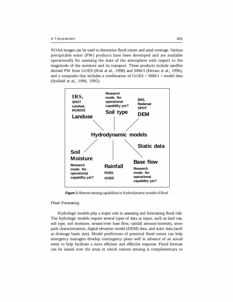
A.T. Jeyaseelan 305
NOAA images can be used to determine flood extent and areal coverage. Variousprecipitable water (PW) products have been developed and are availableoperationally for assessing the state of the atmosphere with respect to themagnitude of the moisture and its transport. These products include satellitederived PW from GOES (Holt et al., 1998) and SSM/I (Ferraro et al., 1996),and a composite that includes a combination of GOES + SSM/I + model data(Scofield et al., 1996, 1995).
Flood Forecasting
Hydrologic models play a major role in assessing and forecasting flood risk.The hydrologic models require several types of data as input, such as land use,soil type, soil moisture, stream/river base flow, rainfall amount/intensity, snowpack characterization, digital elevation model (DEM) data, and static data (suchas drainage basin size). Model predictions of potential flood extent can helpemergency managers develop contingency plans well in advance of an actualevent to help facilitate a more efficient and effective response. Flood forecastcan be issued over the areas in which remote sensing is complementary to
Figure 2: Remote sensing capabilities in Hydrodynamic models of flood
Hydrodynamic models
SoilMoistureResearchmode. Nooperationalcapability yet?
RainfallPOES
GOES
Base flowResearchmode. Nooperationalcapability yet?
Static data
ERS,RadarsatSPOT
DEM
Researchmode. Nooperationalcapability yet?
Soil type
IRS,SPOTLandsat,IKONOS
Landuse
306 Droughts & Floods Assessment and Monitoring
direct precipitation and stream flow measurements, and those areas that arenot instrumentally monitored (or the instruments are not working or are inerror). In this second category, remote sensing provides an essential tool.
Quantitative Precipitation Estimates (QPE) and Forecasts (QPF) usesatellite data as one source of information to facilitate flood forecasts. Newalgorithms are being developed that integrate GOES precipitation estimates,with the more physically based POES microwave estimates. An improvementin rainfall spatial distribution measurements is being achieved by integratingradar, rain gauges and remote sensing techniques to improve real time floodforecasting (Vicente and Scofield, 1998). For regional forecast, the essentialinput data are geomorphology, hydrological analysis, and historical investigationof past events and climatology. GOES and POES weather satellites can provideclimatological information on precipitation especially for those areas notinstrumentally monitored.
Forecast on the local scale requires topography, hydraulic data, riverbedroughness, sediment grain size, hydraulic calculations, land cover, and surfaceroughness. Remote sensing may contribute to mapping topography (generationof DEMs) and in defining surface roughness and land cover. In this case, remotesensing may contribute to updating cartography for land use and DEM.Complex terrain and land use in many areas result in a requirement for veryhigh spatial resolution data over very large areas, which can only be practicallyobtained by remote sensing systems. There is also a need to develop andimplement distributed hydrological models, in order to fully exploit remotelysensed data and forecast and simulate stream flow (Leconte and Pultz, 1990and Jobin and Pultz, 1996). Data from satellites such as ERS, RADARSAT,SPOT and IRS can provide DEM data at resolutions of about 3 to 10 meters.Land use information can be determined through the use of AVHRR, Landsat,SPOT and IRS data. The rainfall component can be determined through theuse of existing POES and GOES platforms. Although there are no operationaldata sources for estimating soil type, soil moisture, snow water equivalent andstream/river base flow, there has been considerable research on the extraction ofthese parameters from existing optical and microwave polar orbiting satellites.
Models can also assist in the mitigation of coastal flooding. Wave run-upsimulations can help planners determine the degree of coastal inundation to beexpected under different, user-specified storm conditions. These types of modelsrequire detailed near-shore bathymetry for accurate wave effect predictions.While airborne sensors provide the best resolution data at present, this datasource can be potentially cost-prohibitive when trying to assess large areas of
A.T. Jeyaseelan 307
coastline. In addition to DEM data, satellite based SAR can also be used toderive near-shore bathymetry for input into wave run-up models on a morecost-effective basis.
Response Phase
Assessment of Flood Damage (immediately during Flood)
The response category can also be called “relief,” and refers to actions takenduring and immediately following a disaster. During floods, timely and detailedsituation reports are required by the authorities to locate and identify the affectedareas and to implement corresponding damage mitigation. It is essential thatinformation be accurate and timely, in order to address emergency situations(for example, dealing with diversion of flood water, evacuation, rescue,resettlement, water pollution, health hazards, and handling the interruptionof utilities etc.). For remote sensing, this often takes the form of damageassessment. This is the most delicate management category since it involvesrescue operations and the safety of people and property.
The following lists information used and analyzed in real time: flood extentmapping and real time monitoring (satellite, airborne, and direct survey),damage to buildings (remote sensing and direct inspections), damage toinfrastructure (remote sensing and direct inspection), meteorologicalNOWCASTS (important real-time input from remote sensing data to showintensity/estimates, movement, and expected duration of rainfall for the next 0- 3 hours), and evaluation of secondary disasters, such as waste pollution, to bedetected and assessed during the crisis (remote sensing and others). In thiscategory, communication is also important to speedy delivery.
Relief (after the Flood)
In this stage, re-building destroyed or damaged facilities and adjustmentsof the existing infrastructure will occur. At the same time, insurance companiesrequire up-to-date information to settle claims. The time factor is not as criticalas in the last stage. Nevertheless, both medium and high-resolution remotesensing images, together with an operational geographic information system,can help to plan many tasks. The medium resolution data can establish theextent of the flood damages and can be used to establish new flood boundaries.They can also locate landslides and pollution due to discharge and sediments.High-resolution data are suitable for pinpointing locations and the degree ofdamages. They can also be used as reference maps to rebuild bridges, washed-out roads, homes and facilities.
308 Droughts & Floods Assessment and Monitoring
Global scenario on Remote Sensing use
There have been many demonstrations of the operational use of thesesatellites for detailed monitoring and mapping of floods and post-flood damageassessment. Remote Sensing information derived from different sensors andplatforms (satellite, airplane, and ground etc.) are used for monitoring floodsin China. A special geographical information system, flood analysis damageinformation system was developed for estimation of real time flood damages(Chen Xiuwan). Besides mapping the flood and damage assessment, high-resolution satellite data were operationally used for mapping post flood riverconfiguration, flood control works, drainage-congested areas, bank erosion anddeveloping flood hazard zone maps (Rao et al., 1998). A variety of satelliteimages of the 1993 flooding in the St. Louis area were evaluated and combinedinto timely data sets. The resulting maps were valuable for a variety of users toquickly locate both natural and man-made features, accurately and quantitativelydetermine the extent of the flooding, characterize flood effects and flooddynamics. (Petrie et al., 1993). Satellite optical observations of floods havebeen hampered by the presence of clouds that resulted in the lack of near real-time data acquisitions. Synthetic Aperture Radar (SAR) can achieve regularobservation of the earth’s surface, even in the presence of thick cloud cover.Therefore, applications such as those in hydrology, which require a regularlyacquired image for monitoring purposes, are able to meet their data requirements.SAR data are not restricted to flood mapping but can also be useful to theestimation of a number of hydrological parameters (Pultz et al., 1996). SARdata were used for estimation of soil moisture, which was used as an input inthe TR20 model for flood forecasting (Heike Bach, 2000). Floods in NorthernItaly, Switzerland, France and England during October 2000 were studiedusing ERS-SAR data. Using information gathered by the European SpaceAgency’s Earth Observation satellites, scientists are now able to study, mapand predict the consequences of flooding with unprecedented accuracy. SARimages are also particularly good at identifying open water - which looks blackin most images. When combined with optical and infra-red photography fromother satellites, an extremely accurate and detailed digital map can be created.Quantitative Precipitation Estimates (QPE) and Forecasts (QPF) use satellitedata as one source of information to facilitate flood and flash flood forecasts inorder to provide early warnings of flood hazard to communities. New algorithmsare being developed that integrate the less direct but higher resolution (spaceand time) images. An improvement in rainfall spatial distribution measurementsis being achieved by integrating radar, rain gauges and remote sensing techniquesto improve real time flood forecasting (Vicente and Scofield, 1998). Potential
A.T. Jeyaseelan 309
gains from using weather radar in flood forecasting have been studied. (U.S.National Report to International Union of Geodesy and Geophysics 1991-1994). A distributed rainfall-runoff model was applied to a 785 km basinequipped with two rain gauges and covered by radar. Data recorded during apast storm provided inputs for computing three flood hydrographs from rainfallrecorded by rain gauges, radar estimates of rainfall, and combined rain gaugemeasurements and radar estimates. The hydrograph computed from thecombined input was the closest to the observed hydrograph. There has beenconsiderable work devoted to developing the approach needed to integrate theseremotely sensed estimates and in situ data into hydrological models for floodforecasting. A large-scale flood risk assessment model was developed for theRiver Thames for insurance industry. The model is based upon airborneSynthetic Aperture Radar data and was built using commonly used GeographicInformation Systems and image processing tools. From the Ortho-rectifiedImages a land cover map was produced (Hélène M. Galy, 2000).
CONCLUSIONS
Droughts and Floods are among the most devastating natural hazards inthe world, claiming more lives and causing extensive damage to agriculture,vegetation, human and wild life and local economies. The remote sensing andGIS technology significantly contributes in the activities of all the three majorphases of drought and flood management namely, 1. Preparedness Phase whereactivities such as prediction and risk zone identification are taken up long beforethe event occurs. 2. Prevention Phase where activities such as Early warning/Forecasting, monitoring and preparation of contingency plans are taken upjust before or during the event and 3. Response/Mitigation Phase where activitiesjust after the event includes damage assessment and relief management. In thislecture, brief review of remote sensing and GIS methods and its utilization fordrought and flood management are discussed.
ACKNOWLEDGEMENTS
The author wishes to thank Dr. R.R. Navalgund, Director, Dr. A.Bhattacharya, Deputy Director (RS &GIS) and Dr. L. Venkataratnam, GroupDirector (A&SG) of NRSA for nominating the author to present the lecture inthe WMO Sponsored Training/Workshop on Remote sensing data interpretationfor Application in Agricultural Meteorology.
310 Droughts & Floods Assessment and Monitoring
REFERENCES
Adler, R.F. and A.J. Negri, 1988. A satellite infrared technique to estimate tropical convectiveand stratiform rainfall. J. Appl. Meteorol., 27: 30-51.
Anagnostou, E.N., A.J. Negri and R.F. Adler, 1999. A satellite infrared technique for diurnalrainfall variability studies. J. Geophy. Res., 104: 31477-31488.
Arkin, P.A. 1979. The relationship between fractional coverage of high cloud and rainfallaccumulations during GATE over the B-scale array. Mon. Wea. Rev., 106: 1153-1171.
ATBD-AST-03, 1996. Advance Space borne Thermal Emission and Reflection Radiometer(ASTER) products.
Barret, E.C. and D.W. Martin, 1981. The use of satellite data in rainfall monitoring. AcademicPress, 340 pp.
Becker, F. 1987. The impact of spectral emissivity on the measurement of land surface temperaturefrom a satellite. Int. J. Remote Sens. 11: 369-394.
Becker, F. and Z.L. Li 1990. Toward a local split window method over land surface. Int. J.Remote Sens. 11: 369-393.
Berk, A., L.S. Bemstein and D.C. Robertson, 1989. MODTRAN: A moderate resolutionmodel for LOWTRAN 7. Rep. GLTR-89-0122, Burlington, MA: Spectral Sciences, Inc.
Chen Xiuwan. Flood Damage Real-Time Estimation-Model based on remote sensing andGIS. Institute of Remote Sensing and GIS, Peking University, Beijing, China. http://incede.iis.u-tokyo.ac.jp/reports/Report_11/Chen.pdf
Colwell, J.E. 1974. Vegetation canopy reflectance. Remote Sens. Environ., 3: 175-183.
Cornette, W.M., P.K. Acharya, D.C. Robertson and G.P. Anderson 1994. Moderate spectralatmospheric radiance and transmittance code (MOSART). Rep. R-057-94(11-30), LaJolla, CA: Photon Research Associates, Inc.
Ferraro, R.R., Weng, F., Grody, N.C. and Basist, A., 1996. An eight year (1987-94) climatologyof rainfall, clouds, water vapor, snowcover, and sea-ice derived from SSM/I measurements.Bull. of Amer. Meteor. Soc., 77: 891-905.
Griffith, C.G., W.L. Woodley, P.G. Grube, D.W. Martin, J. Stout and D.N. Sikdar 1978. Rainestimation from geosynchronous satellite imagery- Visible and infrared studies. Mon.Wea.Rev., 106: 1153-1171.
A.T. Jeyaseelan 311
Gruber, A. 1973. Estimating rainfall in regions of active convection. J. Appl. Meteorol., 12:110-118.
Heike Bach. An Integrated Flood Forecast System Based on Remote Sensing Data, VISTA-Remote sensing applications in Geosciences.
Hélène M. Galy, Richard A. Sanders Willis, London, UK RGS-IBG Annual Conference,University of Sussex, January 4th – 7th 2000.
Holt, F.C., W.P. Menzel, D.G. Gray and T.J. Schmit 1998. Geostationary satellite soundings:new observations for forecasters. US Department of Commerce, NOAA, NESDIS, 30pp.
Hook, S.J., A.R. Gabell, A.A. Green and P.S. Kealy 1992. A comparison of techniques forextracting emissivity information from thermal infrared data for geological studies. RemoteSens. Environ., 42: 123-135.
Jeyaseelan, A.T. and Chandrasekar, K. 2002. Satellite based identification for updation ofDrought prone area in India. ISPRS-TC-VII, International Symposium on Resource andEnvironmental Monitoring, Hyderabad.
Jobin, D.I. and T.J. Pultz, 1996. Assessment of three distributed hydrological models for usewith remotely sensed inputs. Third International Workshop on Applications of RemoteSensing in Hydrology, Greenbelt, MD, October 16-18, pp. 100-130.
Jordan, C.F. 1969. Derivation of leaf area index from quality of light on the forest floor.Ecology, 50: 663-666.
Kahle, A.B. 1986. Surface emittance, temperature and thermal inertia derived from Thermalinfrared multispectral scanner (TIMS) data for Death Valley, California. Geophysics, 52(7): 858-874.
Kahle, A.B., D.P. Madura and J.M. Soha, 1980. Middle infrared multispectral aircraft scannerdata: analysis of geological applications. Appl. Optics, 19: 2279-2290.
Kerr, Y.H., J.P. Lagouarde and J. Imbernon, 1992. Accurate land surface temperature retrievalfrom AVHRR data with use of an improved split window algorithm. Remote Sens.Environ., 41(2-3): 197-209.
Kidder, S.Q. and T.H. Vonder Harr, 1995. Satellite Meteorology: An Introduction. AcademicPress, 466 pp.
Kneizys, F.X., E.P. Shettle, L.W. Abreu, J.H. Chetwynd, G.P. Anderson, W.O. Gallery, J.E. A.Selby and S.A. Clough 1988. Users guide to LOWTRAN7. Rep. AFGL-TR-88-0177,Bedford, MA: Air Force Geophys. Lab.
312 Droughts & Floods Assessment and Monitoring
Kneizys, F.X., E.P. Shettle, W.O. Gallery, J.H. Chetwynd, L.W. Abreu, J.E.A. Selby, S.A.Clough and R.W. Fenn, 1983. Atmospheric transmittance/Radiance: Computer codeLOWTRAN 6. Rep. AFGL-TR-83-0187, Bedford, MA: Air Force Geophys. Lab.
Leconte, R. and T.J. Pultz, 1990. Utilization of SAR data in the monitoring of snowpack,wetlands, and river ice conditions. Workshop on Applications of Remote Sensing inHydrology, Saskatoon, Saskatchewan, February 13-14, 1990, pp. 233-247.
Li, Z.L. and F. Becker, 1993. Feasibility of land surface temperature and emissivity determinationfrom AVHRR data. Remote Sens. Environ, 43: 67-85.
O’Sullivan, F., C.H. Wash, M. Stewart and C.E. Motell, 1990. Rain estimation from infraredand visible GOES satellite data. J. Appl. Meteorol., 29: 209-223.
Ottle, C. and M. Stoll, 1993. Effect of atmospheric absorption and surface emissivity on thedetermination of land temperature from infrared satellite data. Int. J. Remote Sens., 14(10):2025-2037.
Petrie, G.M., G.E. Wukelic, C.S. Kimball, K.L. Steinmaus and D.E. Evaluating 1993.Mississippi River Flood Developments Using ERS-1 SAR, Landsat, and Spot DigitalData. Beaver Pacific Northwest Laboratory, Richland, Washington http://www.odyssey.maine.edu/gisweb/spatdb/acsm/ac94108.html
Prata, A.J. 1994. Land surface temperatures derived from the advanced very high resolutionradiometer and the along track scanning radiometer 2. Expeimental results and validationof AVHRR algorithm. J. Geophys. Res., 99(D6): 13025-13058.
Price, J.C. 1984. Land surface temperature measurements from the split window channels ofthe NOAA-7/AVHRR. J. Geophys. Res., 89: 7231-7237.
Pultz, T.J. and Yves Crevier, 1996. Early demonstration of RADARSAT for applications inhydrology. Third International Workshop on Applications of Remote Sensing inHydrology, Greenbelt, MD, October 16-18, 1996, pp. 271-282.
Rao, D.P., V. Bhanumurthy and G.S. Rao, 1998. Remote Sensing and GIS in FloodManagement in India. Memoir Geological Society of India, No. 41, 1998. pp. 195-218.
Scofield, R.A. and R. Achutuni, 1994. Use of satellite data during the great flood of 1993.Appendix C of the natural disaster survey report on The Great Flood of 1993, NOAA/NWS Report, U.S. Department of Commerce, Silver Spring, MD, C-1 — C-18.
Scofield, R.A. and R. Achutuni, 1996. The satellite forecasting funnel approach for predictingflash floods. Remote Sensing Reviews, 14: 251-282.
A.T. Jeyaseelan 313
Scofield, R.A., D. Zaras, S. Kusselson and R. Rabin, 1996. A remote sensing precipitable waterproduct for use in heavy precipitation forecasting. Proceedings of the 8th Conference onSatellite Meteorology and Oceanography, Atlanta, GA, 29 January - 2 February, 1996,AMS, Boston, MA, pp. 74- 78.
Scofield, R.A., S. Kusselson, D. Olander, and J. Robinson, 1995. Combining GOES, microwave,and raw insonde moisture data for improving heavy precipitation estimates and forecasts.Proceedings of the 14th Conference on Weather Analysis and Forecasting, Dallas, TX, 15– 20 January, 1995, AMS, Boston, MA, (J4) 1 - (J4) 6.
Sobrino, J.A. and V. Caselles, 1991. A methodology for obtaining the crop temperature fromNOAA-9 AVHRR data. Int. J. Remote Sens., 38: 19-34.
Vicente, G. and R.A. Scofield, 1998. The operational GOES infrared rainfall estimationtechnique. Bulletin of the American Meteorological Society, September 1998.
Vidal, A. 1991. Atmospheric and emissivity correction of land surface temperature measuredfrom satellite using ground measurements or satellite data. Int. J. Remote Sens., 12(12):2449-2460.
Wan, Z. and J. Dozier 1996. A generalized split-window algorithm for retrieving land-surfacetemperature from space. IEEE Trans. Geosci. Remote Sens., 34: 892-905.
Wan, Z. and Z.L. Li, 1997. A physics based algorithm for retrieving land-surface emissivityand temperature from EOS/MODIS data. IEEE Trans. Geosci. Remot. Sens., 27(3):268-278.
WATER AND WIND INDUCED SOIL EROSIONASSESSMENT AND MONITORING USINGREMOTE SENSING AND GIS
S.K. SahaAgriculture and Soils DivisionIndian Institute of Remote Sensing, Dehra Dun
Abstract : Water and wind induced soil erosion has adverse economic andenvironmental impacts. Large area in Asia-Pacific region is affected by soil erosion.This paper discusses various satellite remote sensing and GIS based modellingapproaches for soil erosion hazard assessment such as empirical, semi-empirical andprocess based. Few case examples of soil erosion modelling by integrated use ofremote sensing and GIS are included in this article.
INTRODUCTION
Soil degradation by accelerated water and wind-induced erosion is a seriousproblem and will remain so during the 21st century, especially in developingcountries of tropics and subtropics. Erosion is a natural geomorphic processoccurring continually over the earth’s surface. However, the acceleration of thisprocess through anthropogenic perturbations can have severe impacts on soiland environmental quality.
Accelerated soil erosion has adverse economic and environmental impacts(Lal, 1998). Economic effects are due to loss of farm income due to on-siteand off-site reduction in income and other losses with adverse impact on crop/animal production. The on-site and off-site effects of soil erosion onproductivity are depicted in Figure 1 and Figure 2, respectively. Off-siteeconomic impact of soil erosion is presented in Figure 3. Table 1 shows regionalfood production statistics for 1995 with and without soil erosion in the world.The data in Table 1 indicate total loss of food production at 31 M Mg forAfrica, 190 M Mg for Asia and 18 M Mg for tropical America.
Satellite Remote Sensing and GIS Applications in Agricultural Meteorologypp. 315-330
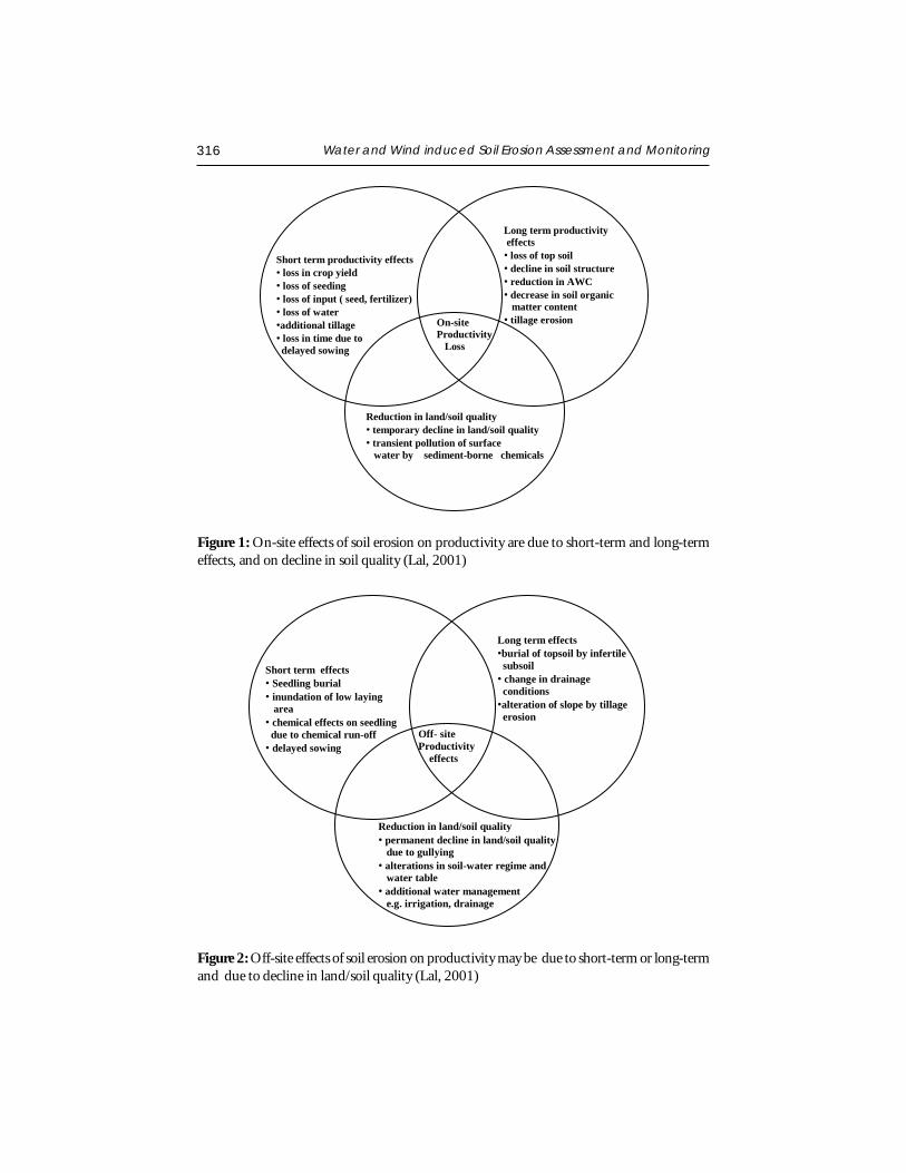
316 Water and Wind induced Soil Erosion Assessment and Monitoring
Figure 1: On-site effects of soil erosion on productivity are due to short-term and long-termeffects, and on decline in soil quality (Lal, 2001)
Figure 2: Off-site effects of soil erosion on productivity may be due to short-term or long-termand due to decline in land/soil quality (Lal, 2001)
Short term productivity effects • loss in crop yield • loss of seeding • loss of input ( seed, fertilizer) • loss of water •additional tillage • loss in time due to delayed sowing
On-site Productivity Loss
Long term productivity effects • loss of top soil • decline in soil structure • reduction in AWC • decrease in soil organic matter content • tillage erosion
Reduction in land/soil quality • temporary decline in land/soil quality • transient pollution of surface water by sediment-borne chemicals
Short term effects • Seedling burial • inundation of low laying area • chemical effects on seedling due to chemical run-off • delayed sowing
Off- site Productivity effects
Long term effects •burial of topsoil by infertile subsoil • change in drainage conditions •alteration of slope by tillage erosion
Reduction in land/soil quality • permanent decline in land/soil quality due to gullying • alterations in soil-water regime and water table • additional water management e.g. irrigation, drainage
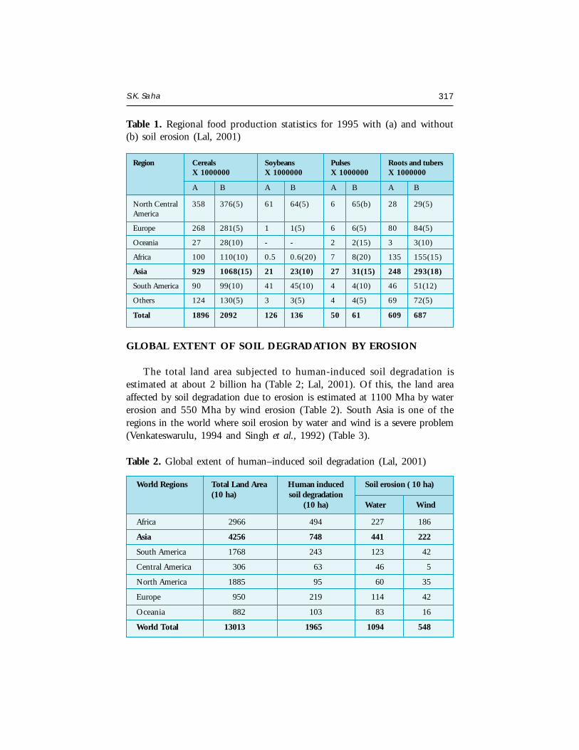
S.K. Saha 317
GLOBAL EXTENT OF SOIL DEGRADATION BY EROSION
The total land area subjected to human-induced soil degradation isestimated at about 2 billion ha (Table 2; Lal, 2001). Of this, the land areaaffected by soil degradation due to erosion is estimated at 1100 Mha by watererosion and 550 Mha by wind erosion (Table 2). South Asia is one of theregions in the world where soil erosion by water and wind is a severe problem(Venkateswarulu, 1994 and Singh et al., 1992) (Table 3).
Table 1. Regional food production statistics for 1995 with (a) and without(b) soil erosion (Lal, 2001)
Region Cereals Soybeans Pulses Roots and tubersX 1000000 X 1000000 X 1000000 X 1000000
A B A B A B A B
North Central 358 376(5) 61 64(5) 6 65(b) 28 29(5)America
Europe 268 281(5) 1 1(5) 6 6(5) 80 84(5)
Oceania 27 28(10) - - 2 2(15) 3 3(10)
Africa 100 110(10) 0.5 0.6(20) 7 8(20) 135 155(15)
Asia 929 1068(15) 21 23(10) 27 31(15) 248 293(18)
South America 90 99(10) 41 45(10) 4 4(10) 46 51(12)
Others 124 130(5) 3 3(5) 4 4(5) 69 72(5)
Total 1896 2092 126 136 50 61 609 687
Table 2. Global extent of human–induced soil degradation (Lal, 2001)
World Regions Total Land Area Human induced Soil erosion ( 10 ha)(10 ha) soil degradation
(10 ha) Water Wind
Africa 2966 494 227 186
Asia 4256 748 441 222
South America 1768 243 123 42
Central America 306 63 46 5
North America 1885 95 60 35
Europe 950 219 114 42
Oceania 882 103 83 16
World Total 13013 1965 1094 548
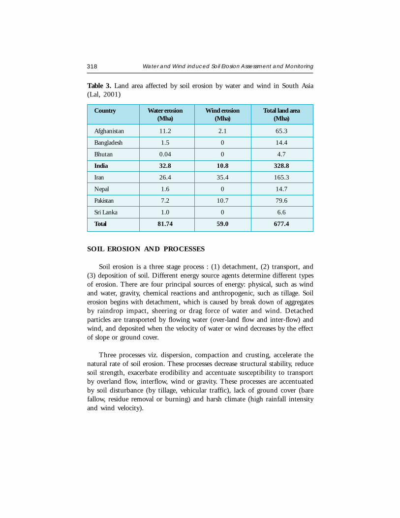
318 Water and Wind induced Soil Erosion Assessment and Monitoring
SOIL EROSION AND PROCESSES
Soil erosion is a three stage process : (1) detachment, (2) transport, and(3) deposition of soil. Different energy source agents determine different typesof erosion. There are four principal sources of energy: physical, such as windand water, gravity, chemical reactions and anthropogenic, such as tillage. Soilerosion begins with detachment, which is caused by break down of aggregatesby raindrop impact, sheering or drag force of water and wind. Detachedparticles are transported by flowing water (over-land flow and inter-flow) andwind, and deposited when the velocity of water or wind decreases by the effectof slope or ground cover.
Three processes viz. dispersion, compaction and crusting, accelerate thenatural rate of soil erosion. These processes decrease structural stability, reducesoil strength, exacerbate erodibility and accentuate susceptibility to transportby overland flow, interflow, wind or gravity. These processes are accentuatedby soil disturbance (by tillage, vehicular traffic), lack of ground cover (barefallow, residue removal or burning) and harsh climate (high rainfall intensityand wind velocity).
Table 3. Land area affected by soil erosion by water and wind in South Asia(Lal, 2001)
Country Water erosion Wind erosion Total land area(Mha) (Mha) (Mha)
Afghanistan 11.2 2.1 65.3
Bangladesh 1.5 0 14.4
Bhutan 0.04 0 4.7
India 32.8 10.8 328.8
Iran 26.4 35.4 165.3
Nepal 1.6 0 14.7
Pakistan 7.2 10.7 79.6
Sri Lanka 1.0 0 6.6
Total 81.74 59.0 677.4
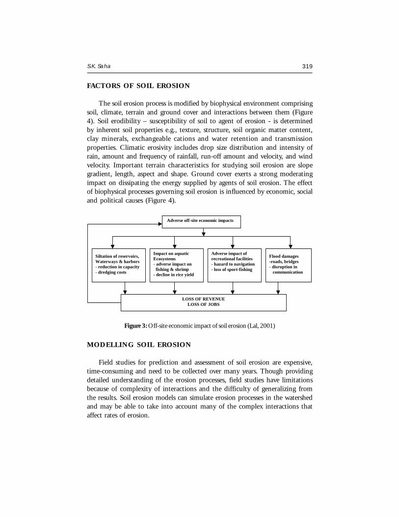
S.K. Saha 319
FACTORS OF SOIL EROSION
The soil erosion process is modified by biophysical environment comprisingsoil, climate, terrain and ground cover and interactions between them (Figure4). Soil erodibility – susceptibility of soil to agent of erosion - is determinedby inherent soil properties e.g., texture, structure, soil organic matter content,clay minerals, exchangeable cations and water retention and transmissionproperties. Climatic erosivity includes drop size distribution and intensity ofrain, amount and frequency of rainfall, run-off amount and velocity, and windvelocity. Important terrain characteristics for studying soil erosion are slopegradient, length, aspect and shape. Ground cover exerts a strong moderatingimpact on dissipating the energy supplied by agents of soil erosion. The effectof biophysical processes governing soil erosion is influenced by economic, socialand political causes (Figure 4).
Figure 3: Off-site economic impact of soil erosion (Lal, 2001)
MODELLING SOIL EROSION
Field studies for prediction and assessment of soil erosion are expensive,time-consuming and need to be collected over many years. Though providingdetailed understanding of the erosion processes, field studies have limitationsbecause of complexity of interactions and the difficulty of generalizing fromthe results. Soil erosion models can simulate erosion processes in the watershedand may be able to take into account many of the complex interactions thataffect rates of erosion.
Adverse off-site economic impacts
Siltation of reservoirs, Waterways & harbors - reduction in capacity - dredging costs
Flood damages -roads, bridges - disruption in communication
Adverse impact of recreational facilities - hazard to navigation - loss of sport-fishing
Impact on aquatic Ecosystems - adverse impact on fishing & shrimp - decline in rice yield
LOSS OF REVENUE LOSS OF JOBS
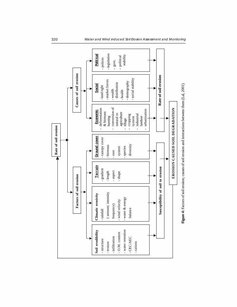
320 Water and Wind induced Soil Erosion Assessment and Monitoring
Figu
re 4
: Fac
tors
of s
oil e
rosi
on; c
ause
s of s
oil e
rosi
on a
nd in
tera
ctio
ns b
etw
een
them
(Lal
, 200
1)
Soil
erod
ibili
ty-
stru
ctur
e- t
extu
re- i
nfilt
ratio
n-
O.M
. con
tent
- wat
er re
tent
ion
- CEC
/AEC
- cat
ions
Clim
atic
ero
sivi
ty- r
ainf
all
( a
mou
nt; i
nten
sity
fre
quen
cy)
- win
d ve
loci
ty- w
ater
& e
nerg
y b
alan
ce
Ter
rain
- gra
dien
t- l
engt
h-
aspe
ct- s
hape
Grou
nd c
over
- can
opy
cove
r- b
iom
ass
- roo
t s
yste
m- s
peci
es d
iver
sity
Econ
omic
-de
fore
stat
ion
& b
iom
ass
burn
ing
-co
nver
sion
of
natu
ral t
oag
ricul
ture
-til
lage
-cr
oppi
ngsy
stem
-in
dust
rial
land
use
-ur
bani
zatio
n
Social
- lan
d rig
ht- m
arke
t for
ces
- wea
lth d
istri
butio
n- h
ealth
- dem
ogra
phy
- soc
ial s
tabi
lity
Polit
ical
- pol
ices
- leg
islat
ion
- go
vt.
- po
litic
al
sta
bilit
y
Rat
e of
soi
l ero
sion
Cau
ses
of s
oil
eros
ion
Fact
ors
of s
oil e
rosi
on
Susc
eptib
ility
of
soil
to e
rosi
onR
ate o
f soi
l ero
sion
ER
OSI
ON
CA
USE
D S
OIL
DE
GR
AD
AT
ION
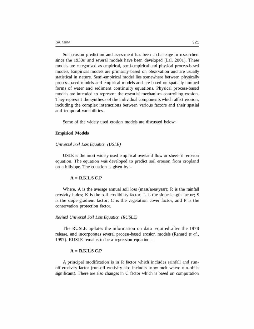
S.K. Saha 321
Soil erosion prediction and assessment has been a challenge to researcherssince the 1930s’ and several models have been developed (Lal, 2001). Thesemodels are categorized as empirical, semi-empirical and physical process-basedmodels. Empirical models are primarily based on observation and are usuallystatistical in nature. Semi-empirical model lies somewhere between physicallyprocess-based models and empirical models and are based on spatially lumpedforms of water and sediment continuity equations. Physical process-basedmodels are intended to represent the essential mechanism controlling erosion.They represent the synthesis of the individual components which affect erosion,including the complex interactions between various factors and their spatialand temporal variabilities.
Some of the widely used erosion models are discussed below:
Empirical Models
Universal Soil Loss Equation (USLE)
USLE is the most widely used empirical overland flow or sheet-rill erosionequation. The equation was developed to predict soil erosion from croplandon a hillslope. The equation is given by –
A = R.K.L.S.C.P
Where, A is the average annual soil loss (mass/area/year); R is the rainfallerosivity index; K is the soil erodibility factor; L is the slope length factor; Sis the slope gradient factor; C is the vegetation cover factor, and P is theconservation protection factor.
Revised Universal Soil Loss Equation (RUSLE)
The RUSLE updates the information on data required after the 1978release, and incorporates several process-based erosion models (Renard et al.,1997). RUSLE remains to be a regression equation –
A = R.K.L.S.C.P
A principal modification is in R factor which includes rainfall and run-off erosivity factor (run-off erosivity also includes snow melt where run-off issignificant). There are also changes in C factor which is based on computation
322 Water and Wind induced Soil Erosion Assessment and Monitoring
of sub-factor called soil loss ratios (SLR). The SLR depends on sub-factors :prior landuse, canopy cover, surface cover, surface roughness and soil moisture(Renard et al., 1997).
Semi-empirical Models
Modified Universal Soil Loss Equation (MUSLE)
Williams (1975) proposed a modified version of USLE that can be writtenas–
Sye = Xe.K.L.S.Ce.Pe
Where, Sye is the event sediment yield
Xe = α. (Qe. qp) 0.56
Where, α is an empirical co-efficient; Qe is the run-off amount and qp isthe peak run-off rate obtained during the erosion event and K.L.S.Ce & Peare as defined for USLE.
Morgan, Morgan and Finney (MMF) Model
Morgan et al. (1984) developed a model to predict annual soil loss whichendeavors to retain the simplicity of USLE and encompasses some of the recentadvances in understanding of erosion process into a water phase and sedimentphase. Sediment phase considers soil erosion to result from the detachmentof soil particles by overland flow. Thus, the sediment phase comprises twopredictive equations, one for rate of splash detachment and one for thetransport capacity of overland flow. The model uses six operating equationsfor which 15 input parameters are required (Table 4). The model comparespredictions of detachment by rain splash and the transport capacity of therun-off and assesses the lower of the two values as the annual rate of soil loss,thereby denoting whether detachment or transport is the limiting factor.
Physical Process-based Model
Empirical models have constraints of applicability limited to ecologicalconditions similar to those from which data were used in their development.
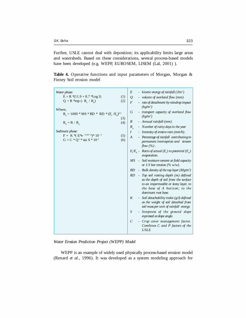
S.K. Saha 323
Further, USLE cannot deal with deposition; its applicability limits large areasand watersheds. Based on these considerations, several process-based modelshave been developed (e.g. WEPP, EUROSEM, LISEM (Lal, 2001) ).
Table 4. Operative functions and input parameters of Morgan, Morgan &Finney Soil erosion model
Water Erosion Prediction Project (WEPP) Model
WEPP is an example of widely used physically process-based erosion model(Renard et al., 1996). It was developed as a system modeling approach for
E - kinetic energy of rainfall (J/m2)
Q - volume of overland flow (mm)
F - rate of detachment by raindrop impact(kg/m2)
G - transport capacity of overland flow(kg/m2)
R - Annual rainfall (mm)
Rn
- Number of rainy days in the year
I - Intensity of erosive rain (mm/h).
A - Percentage of rainfall contributing topermanent interception and streamflow (%) .
Et/E
0- Ratio of actual (E
t) to potential (E
0)
evaporation.
MS - Soil moisture content at field capacityor 1/3 bar tension (% w/w).
BD - Bulk density of the top layer (Mg/m3)
RD - Top soil rooting depth (m) definedas the depth of soil from the surfaceto an impermeable or stony layer, tothe base of A horizon; to thedominant root base.
K - Soil detachability index (g/J) definedas the weight of soil detached fromsoil mass per unit of rainfall energy.
S - Steepness of the ground slopeexpressed as slope angle.
C - Crop cover management factor.Combines C and P factors of theUSLE
Water phase:E = R *(11.9 + 8.7 *Log I) (1)Q = R *exp (- R
C / R
0) (2)
Where,R
C = 1000 * MS * BD * RD * (E
t /E
0)0.5
(3)R
0 = R / R
n(4)
Sediment phase:F = K *( E*e – 0.05* A)* 10 –3 (5)G = C * Q2 * sin S * 10-3 (6)
324 Water and Wind induced Soil Erosion Assessment and Monitoring
predicting and estimating soil loss and selecting catchment managementpractices for soil conservation. Basic erosion and deposition equations in WEPPare based on the mass balance formulation that uses rill and inter-rill conceptof soil erosion, which is a steady-state sediment continuity equation. TheWEPP model computes erosion by rill and inter-rill processes. The sedimentdelivery to rill from inter-rill is computed by following equation –
Di = Ki. Ie2. Ge. Ce. Sf
Where, Di is the delivery of sediment from inter-rill areas to rill (kg/m2/sec); Ki is the inter-rill erodibility (kg/m4/sec); Ie is the effective rainfallintensity (m/sec.); Ge is the ground cover adjustment factor and Sf is the slopeadjustment factor calculated as per equation given below –
Sf = 1.05 – 0.85 exp ( -4 Sin α )
Where, α is the slope of the surface towards nearby rill. In comparison,rill erosion is the detachment and transport of soil particles by concentratedflowing water -
Dc = Kr. ( T - Tc)
Where, Kr is the rill erodibility (sec/m); T is the hydraulic shear of flowingwater (Pa) and Tc is the critical hydraulic shear that must be exceeded beforerill detachment can occur (Pa).
Wind Erosion Model
Comparable to the USLE, a wind erosion model was proposed by Woodruffand Siddoway (1965) as shown in equation given below –
E = f (I, K, C, L, V)
Where, E is the mean annual wind erosion; I is the soil erodibility index;C is the climatic factor (Wind energy); L is the unsheltered median traveldistance of wind across a field; V is the equivalent vegetative cover. Thisequation has been widely adopted and used for estimating erosion hazard indry lands.
S.K. Saha 325
USE OF SATELLITE REMOTE SENSING AND GIS IN SOIL EROSIONMODELING
The potential utility of remotely sensed data in the form of aerialphotographs and satellite sensors data has been well recognized in mappingand assessing landscape attributes controlling soil erosion, such as physiography,soils, land use/land cover, relief, soil erosion pattern (e.g. Pande et al., 1992).Remote Sensing can facilitate studying the factors enhancing the process, suchas soil type, slope gradient, drainage, geology and land cover. Multi-temporalsatellite images provide valuable information related to seasonal land usedynamics. Satellite data can be used for studying erosional features, such asgullies, rainfall interception by vegetation and vegetation cover factor. DEM(Digital Elevation Model) one of the vital inputs required for soil erosionmodeling can be created by analysis of stereoscopic optical and microwave(SAR) remote sensing data.
Geographic Information System (GIS) has emerged as a powerful tool forhandling spatial and non-spatial geo-referenced data for preparation andvisualization of input and output, and for interaction with models. There isconsiderable potential for the use of GIS technology as an aid to the soilerosion inventory with reference to soil erosion modeling and erosion riskassessment.
Erosional soil loss is most frequently assessed by USLE. Spanner et al.(1982) first demonstrated the potential of GIS for erosional soil loss assessmentusing USLE. Several studies showed the potential utility of RS and GIStechniques for quantitatively assessing erosional soil loss (Saha et al., 1991;Saha and Pande, 1993; Mongkosawat et al., 1994). Satellite data analyzedsoil and land cover maps and DEM derived and ancillary soil and agro-climaticrainfall data are the basic inputs used in USLE for computation of soil loss.Kudrat and Saha (1996) showed the feasibility of GIS to estimate actual andpotential sediment yields following Sediment Yield Prediction Equation (SYPE)using RS derived soil and land use information, DEM derived slope andancillary rainfall and temperature data. MMF model was used for quantificationof soil loss by water erosion in Doon Valley, Dehra Dun, India, in GISenvironment using various satellite remote sensing derived inputs (ASD, 2002).
The availability of GIS tools and more powerful computing facilities makesit possible to overcome difficulties and limitations and to develop distributed
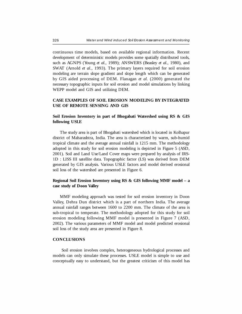
326 Water and Wind induced Soil Erosion Assessment and Monitoring
continuous time models, based on available regional information. Recentdevelopment of deterministic models provides some spatially distributed tools,such as AGNPS (Young et al., 1989); ANSWERS (Beasley et al., 1980), andSWAT (Arnold et al., 1993). The primary layers required for soil erosionmodeling are terrain slope gradient and slope length which can be generatedby GIS aided processing of DEM. Flanagan et al. (2000) generated thenecessary topographic inputs for soil erosion and model simulations by linkingWEPP model and GIS and utilizing DEM.
CASE EXAMPLES OF SOIL EROSION MODELING BY INTEGRATEDUSE OF REMOTE SENSING AND GIS
Soil Erosion Inventory in part of Bhogabati Watershed using RS & GISfollowing USLE
The study area is part of Bhogabati watershed which is located in Kolhapurdistrict of Maharashtra, India. The area is characterized by warm, sub-humidtropical climate and the average annual rainfall is 1215 mm. The methodologyadopted in this study for soil erosion modeling is depicted in Figure 5 (ASD,2001). Soil and Land Use/Land Cover maps were prepared by analysis of IRS-1D : LISS III satellite data. Topographic factor (LS) was derived from DEMgenerated by GIS analysis. Various USLE factors and model derived erosionalsoil loss of the watershed are presented in Figure 6.
Regional Soil Erosion Inventory using RS & GIS following MMF model – acase study of Doon Valley
MMF modeling approach was tested for soil erosion inventory in DoonValley, Dehra Dun district which is a part of northern India. The averageannual rainfall ranges between 1600 to 2200 mm. The climate of the area issub-tropical to temperate. The methodology adopted for this study for soilerosion modeling following MMF model is presented in Figure 7 (ASD,2002). The various parameters of MMF model and model predicted erosionalsoil loss of the study area are presented in Figure 8.
CONCLUSIONS
Soil erosion involves complex, heterogeneous hydrological processes andmodels can only simulate these processes. USLE model is simple to use andconceptually easy to understand, but the greatest criticism of this model has
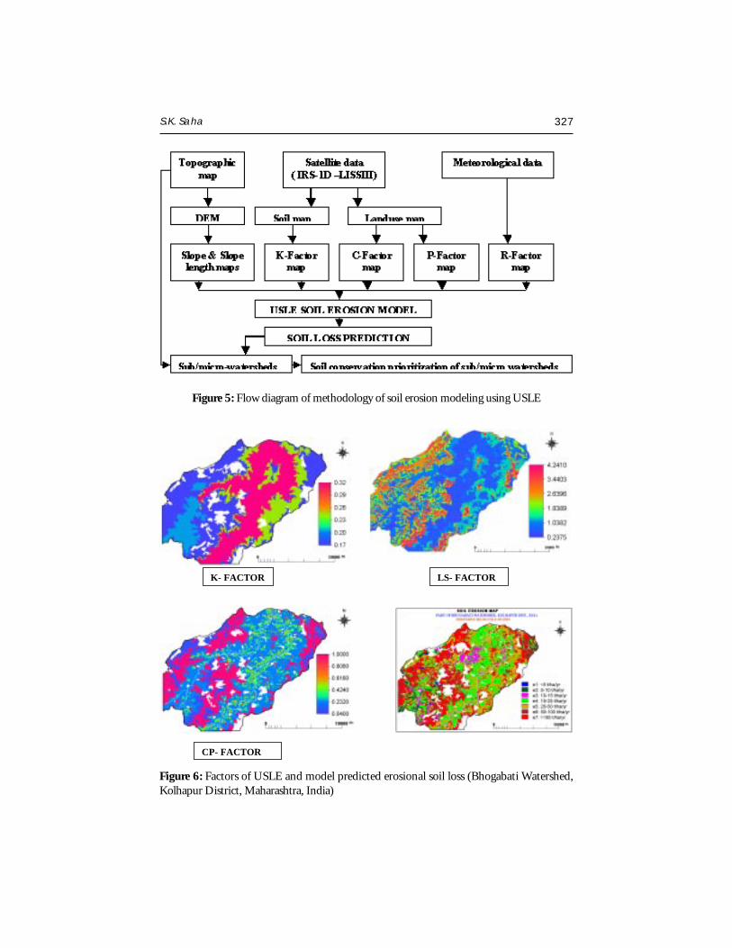
S.K. Saha 327
Figure 5: Flow diagram of methodology of soil erosion modeling using USLE
K- FACTOR LS- FACTOR
CP- FACTOR
Figure 6: Factors of USLE and model predicted erosional soil loss (Bhogabati Watershed,Kolhapur District, Maharashtra, India)
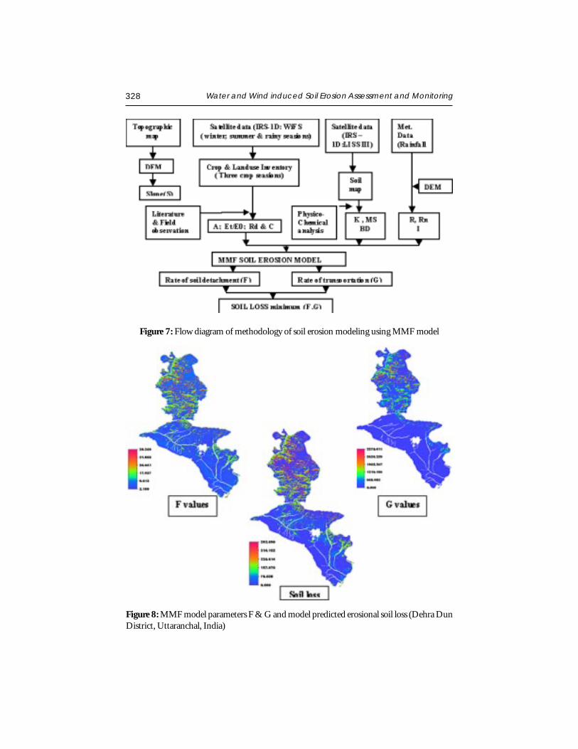
328 Water and Wind induced Soil Erosion Assessment and Monitoring
Figure 7: Flow diagram of methodology of soil erosion modeling using MMF model
Figure 8: MMF model parameters F & G and model predicted erosional soil loss (Dehra DunDistrict, Uttaranchal, India)
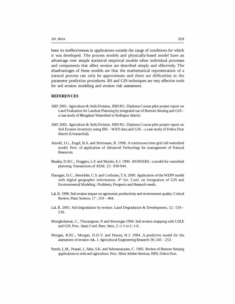
S.K. Saha 329
been its ineffectiveness in applications outside the range of conditions for whichit was developed. The process models and physically-based model have anadvantage over simple statistical empirical models when individual processesand components that affect erosion are described simply and effectively. Thedisadvantages of these models are that the mathematical representation of anatural process can only be approximate and there are difficulties in theparameter prediction procedures. RS and GIS techniques are very effective toolsfor soil erosion modeling and erosion risk assessment.
REFERENCES
ASD 2001. Agriculture & Soils Division, IIRS P.G. Diploma Course pilot project report onLand Evaluation for Landuse Planning by integrated use of Remote Sensing and GIS –a case study of Bhogabati Watershed in Kolhapur district.
ASD 2002. Agriculture & Soils Division, IIRS P.G. Diploma Course pilot project report onSoil Erosion Inventory using IRS – WiFS data and GIS – a case study of Dehra Dundistrict (Uttaranchal).
Arnold, J.G., Engel, B.A. and Srinivasan, R. 1998. A continuous time grid cell watershedmodel. Proc. of application of Advanced Technology for management of NaturalResources.
Beasley, D.B.C., Huggins, L.F. and Monke, E.J. 1990. ANSWERS : a model for watershedplanning. Transactions of ASAE. 23 : 938-944.
Flanagan, D.C., Renschler, C.S. and Cochrane, T.A. 2000. Application of the WEPP modelwith digital geographic information. 4th Int. Conf. on Integration of GIS andEnvironmental Modeling : Problems, Prospects and Research needs.
Lal, R. 1998. Soil erosion impact on agronomic productivity and environment quality: CriticalReview. Plant Science, 17 : 319 – 464.
Lal, R. 2001. Soil degradation by erosion. Land Degradation & Development, 12 : 519 –539.
Mongkolsawat, C., Thurangoon, P. and Sriwongsa 1994. Soil erosion mapping with USLEand GIS. Proc. Asian Conf. Rem. Sens., C-1-1 to C-1-6.
Morgan, R.P.C., Morgan, D.D.V. and Finney, H.J. 1984. A predictive model for theassessment of erosion risk. J. Agricultural Engineering Research 30: 245 – 253.
Pande, L.M., Prasad, J., Saha, S.K. and Subramanyam, C. 1992. Review of Remote Sensingapplications to soils and agriculture. Proc. Silver Jubilee Seminar, IIRS, Dehra Dun.
330 Water and Wind induced Soil Erosion Assessment and Monitoring
Renard, K.G., Foster, G.R., Lane, I.J. and Laflen, J.M. 1996. Soil loss estimation. In SoilErosion, Conservation and Rehabilitation; Agassi, M. (ed.). Marcel Dekkar, New York,169-202.
Renard, K.G., Foster, G.R., Weesies, G.A., Mc Cool, D.K. and Yoder, D.C. 1997. Predictingsoil erosion by water : A guide to conservation planning with the revised USLE. USDAHand Book No. 703, USDA, Washington, D.C.
Saha, S.K. and Pande, L.M. 1993. Integrated approach towards soil erosion inventory forenvironmental conservation using satellite and agro-meteorological data. Asia-Pacific Rem.Sens. J., 5(2) : 21-28.
Saha, S.K., Kudrat, M. and Bhan, S.K. 1991. Erosional soil loss prediction using digitalsatellitee data and USLE, pages 369-372. In Applications of Remote Sensing in Asiaand Oceania – environmental change monitoring (Shunji Murai ed.). Asian Associationof Remote Sensing.
Spanner, M.A., Strahler, A.H. and Estes, J.E. 1982. Proc. Int. Symp. Rem. Sens. Environ.,Michigan, USA.
Singh, G., Babu, R., Narain, P., Bhushan, L.S. and Abrol, I.P. 1992. Soil erosion rates inIndia. J. Soil Water Conservation, 47 : 93 – 95.
Venkateswarlu, J. 1994. Managing extreme stresses in arid zone of Western Rajasthan, India.In Stressed Ecosystem and Sustainable Agriculture. Virmani, S.M.; Katyal, J.C.; Eswaran,H. and Abrol, I.P. (eds.). Oxford & IBH Publishing, New Delhi, p. 161-171.
Williams, R. 1975. Sediment Yield Prediction with USLE using run-off energy factor. InPresent and prospective technology for predicting sediment yields and sources. ARS-S-40, USDA, Washington D.C. : 244-252.
Woodruff, N.P. and Siddoway, F..H. 1965. A wind erosion equation. Soil Sci. Soc. Am. Proc.,29 : 602-608.
Young, R.A., Onstad, C.A., Bosch, D.D. and Anderson, W.P. 1989. AGNPS – Agriculture-Non-Point Source Pollution Model : A watershed analysis tool. Conservation Res. Report35, USDA, ARS, Morris, MN, USA.
Zhang, L. 1994. A comparison of the efficiency of the three models to estimate water yieldchanges after forced catchment conversion. M.Sc. (Forest) Thesis, University ofMelbourne, Australia.
SATELLITE BASED WEATHER FORECASTING
S.R. KalsiIndia Meteorological DepartmentMausam Bhawan, Lodi Road, New Delhi
Abstract : Satellite data are increasingly being used in conjunction with conventionalmeteorological observations in the synoptic analysis and conventional weatherforecast to extract information of relevance for agriculture in India. Synopticapplications of satellite imagery as in use at India Meteorological Department arehighlighted in this report. Particular emphasis is laid on identification of large scaleconvective precipitation systems such as monsoon depressions and tropical cyclones.A brief review of national and international satellite systems of relevance to weatherforecasts particularly for agriculture is provided. A summary of numerical productsbeing derived from satellite data and their use in numerical models is also given. A
brief on the New long range forecasting technique is included.
INTRODUCTION
Reliable weather prediction holds the key for socio economic developmentand is essential for food security of the human society. Since time immemorial,human race has been fascinated by the ever changing and highly dynamicatmosphere around him and has made concerted efforts to understand thecontrolling processes and achieve better capabilities of weather forecasting. Therecent attempts for satellite based observations, made over the past two decades,have provided new insights in these processes. Synoptic coverage provided bysatellites is ideally suited to study weather related atmospheric processes ondifferent scales. The recent advances in satellite technology in terms of highresolution, multi-spectral bands covering visible, infrared and microwaveregions have made space data an inevitable component in weather monitoringand dynamic modeling. The impact of satellite data is phenomenal in certainareas of meteorological applications such as short-range forecasts, TropicalCyclone (TC) monitoring, aviation forecasts etc. With improving trend inaccuracy of satellite retrievals, improvements could be carried out in modelsleading to improved forecasts, especially in the tropics.
Satellite Remote Sensing and GIS Applications in Agricultural Meteorologypp. 331-346
332 Satellite Based Weather Forecasting
CONTRIBUTIONS OF SPACE OBSERVATIONS
The launch of the first meteorological satellite TIROS-1 in April 1960heralded the era of Space observations and gave the first glimpses of thedynamic cloud systems surrounding the Earth. Since then the technology hasdeveloped by leaps and bounds in observation capabilities in terms of spatial,spectral and temporal resolutions. A global system of Space observations withboth geostationary and polar orbiting satellites has evolved.
The advantages of Space observations emanate from several factors suchas:
Synoptic view of large areas, bringing out the inter-relations of processesof different spatial scales.
Frequent observations from geostationary satellites provide continuousmonitoring while polar orbiting satellites give typical twice daily coverage;such data is relevant for study of weather system dynamics.
The inherent spatial averaging is more representative than the point in-situ observations and readily usable for weather prediction models.
High level of uniformity of space observations overcomes the problem ofinter-calibration needed for ground based instruments.
Filling of gaps in observations; Space data covers large oceanic areas andinaccessible and remote land areas, thus giving global coverage.
New types of data and observations; parameters such as sea surface (skin)temperature, sea surface wind stress, sea level, cloud liquid water content,radiation balance, aerosol are some of the unique parameters provided onlyby satellites.
Simultaneous observation of several dynamic parameters provided bydifferent sensors in same platform facilitates study of inter-relationshipsand knowledge of processes (e.g. Sea Surface temperature and deepconvection, cloud development and radiative forcing ).
METEOROLOGICAL SATELLITES / PAYLOADS
Currently several operational meteorological satellites are providing globaland regional observations. Six different types of satellite systems currently in
S.R. Kalsi 333
use are : 1) Visible/ Infrared/Water Vapour Imagers, 2) Infrared Sounders, 3)Microwave Imagers, 4) Microwave Sounders, 5) Scatterometers and 6) RadarAltimeters. Though the water vapour imaging capability is available only onthe geostationary satellite, the visible and infrared imagers are available ongeostationary as well as polar orbiting satellites. The last four are currentlyavailable only on polar orbiting systems. We first describe in detail below theINSAT system which is the primary satellite for weather surveillance in thispart of the globe. It is a multipurpose geostationary satellite that caters tothe requirements of Meteorology and Communication. It carries a met payloadcalled Very High Resolution Radiometer ( VHRR ) that enables us to havevisible, infrared and now even water vapour images. It is designed to providethe following services:
Round the clock surveillance of weather systems including severe weatherevents around the Indian region.
Operational parameters for weather forecasting – cloud cover, cloud toptemperature, sea surface temperature, snow cover, cloud motion vector,outgoing long wave radiation etc.
Collection and transmission of meteorological, hydrological andoceanographic data from remote/inaccessible areas through Data CollectionPlatforms.
Timely dissemination of warning of impending disasters such as cyclonesthrough Cyclone Warning Dissemination Systems.
Dissemination of Meteorological information including processed imagesof weather systems through Meteorological Data dissemination system.
INSAT applications programme started with the launch of INSAT-1 seriesof satellites in early 1980s. INSAT-2 series that followed was designed basedon user feedback. INSAT-2A and 2B launched in 1992 and 1993 carriedVHRR payload with improved resolution of 2 km in visible and 8 km inthermal band. The imaging capability included three modes, viz. full frame,normal mode and sector mode of 5 minutes for rapid coverage of severeweather systems.
INSAT-2E launched in 1999 carried an advanced VHRR payload operatingin three channels – visible (2 km), thermal and water vapour (8 km). Thewater vapour channel is capable of giving water vapour distribution and flow
334 Satellite Based Weather Forecasting
patterns in the middle troposphere. Besides this, INSAT-2E also carried a CCDcamera with 3 channels – visible, near infrared and short wave infrared with1 km resolution to map the vegetation cover.
A geostationary meteorological satellite (METSAT) system devoted totallyto meteorology was launched in 2002. It has been renamed as Kalpana-1 andis currently the operational satellite system being used by IMD.
INSAT-3A has been launched in April 2003 and carries identical payloadsas in INSAT-2E. INSAT- 3D planned for future will also carry atmosphericsounder for temperature and water vapour profiles and split thermal channelsfor accurate sea surface temperature retrieval. Data from INSAT satellites arebeing used to retrieve a number of quantitative products. INSAT imagery isbeing used very exhaustively to provide support for synoptic analysis andweather forecasting. The quantitative products available from INSAT and itsapplications are described in subsequent sections.
Infrared Sounders
These systems are available on geostationary (GEOS N SERIES) and polarorbiting (NOAA 15-17/HIRS) Satellites. The primary application lies in directassimilation of IR radiance in NWP models. IR sounders are going to have (2orders of Magnitude) increase in the infrared channels. This will lead to largeimprovements in the vertical resolution of derived temperature and moistureprofiles in clear areas and above cloud top level and improve the initialtemperature and moisture fields.
Microwave Sounders
Similar to the microwave imager data, microwave sounder data fromNOAA-15-17/AMSU instrument can provide valuable information belowcloud top level. Tropospheric thermal measurements can be obtained in non-raining cloudy region. Microwave sounders data has proved to be very usefulin determining upper tropospheric warm anomaly. This in turn is used indiagnosing intensity and intensity change of tropical cyclones ( Brueske andVelden, 2000).
Microwave Imagers
VIS and IR provide proxy variables. Exact positioning of the eye is possiblein VIS and IR imagery. Microwave (passive) sensors monitor radiation from
S.R. Kalsi 335
below the cirrus shield and provide information on atmospheric WV, cloudliquid water, precipitation, intensity and regions of convective activity. In Juneof 1987 the first satellite from the Defence Meteorological SatelliteProgramme (DMSP) carrying a microwave radiometer called Special SensorMicrowave/Image (SSM/I) was launched. It overlapped with the EuropeanResearch Satellite (ERS-I) launched in July 1991 which carried a scatterometer.The swath width of the ERS-I scatterometer was only 500 km resulting,however, in the less than-complete coverage of the tropical regions each day.
The low horizontal resolution of some current radiometers may limit theusefulness of some parameters but the 15 km resolution of 85 GHz channelof SSM/I provides meso-scale information. This channel provides radar likeimagery and is able to discern the circulation centres. Velden et al. (1989)describe the advantage of centre-fixing in TCs using 85 GHz imagerycompared to conventional VIS and IR images where centres are covered incirrus overcast. NASA launched a special satellite that aimed at making newmeasurements of meteorological quantities in the tropics. The Tropical RainfallMeasuring Mission (TRMM) has completed 3 years of successful data takingin 2000. With the change of its altitude from 350 km to 400 km, it willhave enough fuel to provide continuous measurements upto 2005 (Veldenand Hawkins, 2002). TRMM Microwave Imager (TMI) provides horizontalresolution of 5-7 km for 85 GHz channel which is 2-3 times better than theSSM/I, and the higher resolution TMI 37 GHz channel; can penetrate deeperinto tropical cyclone to reveal additional details.
The Indian Remote Sensing Satellite (IRS-P4) launched in 1999 carriedMultichannel Scanning Microwave Radiometer (MSMR). It is providingmeasurements at 6.6, 10, 18 and 21 GHz frequencies in both H&Vpolarizations. Attempts have been made to provide estimates of integrated watervapour, liquid water content, precipitation intensity, and SSTs over the globaloceans (Gohil et al., 2001).
Scatterometers
The primary application of the scatterometers is for Ocean Surface WindVectors. A scatterometer sends microwave pulses to the earth’s surface andmeasures the backscattered power from the surface roughness elements. Theback scatter power depends not only on the magnitude of the wind stress butalso on the wind direction relative to the direction of the radar beam. Therelation between backscatter signal and ocean surface winds is not well
336 Satellite Based Weather Forecasting
established under the strong wind and rainy conditions of a cyclone becauseof lack of validation. After the failure of NASA’s NSCAT system, there hasbeen rapid deployment of a new system called Quikscat that provides a wideswath of 1800 km and unprecedented global ocean coverage. Wind fields fromquikscat are available on near real-time to most TC forecast offices. The standardwind product has a 25 km spatial resolution. The data has provided the outerwind structure of tropical cyclones. It is also used to determine the radius of35 knots (De Muth et al., 2001), and for identifying closed circulations ofdeveloping systems and in providing lower limits for maximum sustainedwinds. Sarkar (2003) has reviewed techniques for surface wind measurementsover global oceans from space platforms. The most successful wind sensor hasbeen the microwave scatterometer.
Radar Altimeters
Many studies have shown that sub-surface thermal structure plays animportant role in tropical cyclone intensification. The sub-surface structurecan often be deduced from the satellite altimetry data. Research to better usethese data in statistical forecast algorithms and the coupled ocean-atmospheremodels has the potential to improve tropical cyclone intensity forecasts. Thealtimeter observations would be more useful with improved temporal and arealsampling. Multi-beam altimeters potentially can dramatically increase spatialsampling and fill the data voids.
SYNOPTIC APPLICATIONS IN IMD
The major application of satellite data has been the monitoring of Synopticweather systems ranging from thunderstorms to cyclones and planetary scalephenomena such as monsoon. The dynamic nature of weather systems couldbe captured through the time series of satellite observations leading to betterunderstanding of the process of genesis, growth and decay. This has led tosatellite based technique (Dvorak technique) to assess the intensity of TCaccurately and estimate the growth potential. The specific applications includeidentification of primary weather system such as low pressure, depression,troughs/ridges, jet streams regions of intensive convection, inter-tropicalconvergence zones etc. and onset and progress of monsoon system.
Following are the major applications of satellites images in operationalweather forecasting:
S.R. Kalsi 337
i. Watch and monitor growth of weather phenomena like cumulonimbuscells, thunderstorm, fog etc. and their decay.
ii. Identify and locate primary synoptic systems like troughs/ridges, jetstreams, regions of intense convection, inter tropical convergence zonesetc.
iii. Monitor onset and progress of monsoon systems.
iv. Detect genesis and growth of TC and monitor their intensificationand movement till landfall. This application is included in the nextsection.
Satellite imagery is being extensively used by synoptic network inconjunction with other available conventional meteorological data for analysisand weather forecasting. Zones of cloudiness are identified from the satelliteimagery as regions of upward velocity and hence potential areas for occurrenceof rainfall. Visible, infra red and water vapour images have distinctive usesand are complementary to each other.
We shall summarize below very briefly some of the very importantapplications in the operational synoptic analysis and weather forecasting.
Satellite imagery is very handy for remote and inaccessible areas such asHimalayas where heavy precipitation usually builds up. Though thecharacteristic cloud patterns of cold and warm fronts are not seen over India,the Western disturbances giving rise to heavy snow fall are well captured inthe Satellite imagery (Kalsi and Mishra, 1983). The Cloud band ahead of wellmarked westerly trough is clearly seen in the Satellite imagery. Thecharacteristic structure of snow is easily identified and its areal extent ismonitored for estimating run-off and also for long range prediction ofmonsoon.
Deep penetrative CB clouds and thunderstorm complexes (Kalsi andBhatia, 1992) are rather easy to be identified in visible and infrared imagery.Squall lines are clearly seen in the satellite loops. Satellite imagery providespowerful signals for forecasting severe weather (Purdom, 2003).
The rain bearing Southwest monsoon system advances northward usuallyas an intermittent band of cloudiness called inter-tropical convergence zone(ITCZ). It comprises of numerous rain showers and thunderstorms associatedwith the convergence in the shear zone. One of the earliest studies (Sikka &
338 Satellite Based Weather Forecasting
Gadgil, 1980) showed the 30-40 day oscillatory nature of monsoon flow. TheINSAT and NOAA sounding data have brought out the unique nature ofmonsoon onset with large scale changes in wind and moisture profiles in lowertroposphere prior to monsoon onset. Using satellite data Joshi et al. (1990)have also noted a spectacular rise in the 300 mb temperature over the westerncentral and eastern Tibetan Plateau and over the region of the heat low overPakistan. They noted this rise commencing almost 2 weeks prior to the onsetof monsoon rains over southwestern India. This appears to be an importantparameter for monitoring the onset of monsoons and requires to be monitoredin connection with forecast of the onset of monsoon operationally. Josephet al. (2003) have identified conditions leading to onset of monsoon overKerala using SST, OLR and winds obtained from satellite systems.
The monsoon depressions are the principal rain bearing systems of thesouthwest monsoon period over India. Substantial amounts of rainfall aregenerated by the westward passage of monsoon depressions forming in thebay. Monsoon depressions usually develop from innocuous looking cloudsystems and from diffuse pressure fields over the head Bay of Bengal. Satelliteimagery shows heavy overcast cloud mass in the southern sector with low levelcumulus clouds determining the Low-Level Circulation Centre (LLCC) to thenortheast. The LLCC is often free of deep convection. The widespread andheavy rainfall in the southwest sector is often accompanied with deepconvection in that sector. Kalsi et al. (1996) have shown from satellite imagerythat a few of these depressions acquire structure of marginal cyclones withalmost vertical structure upto mid-tropospheric levels. Following Scoffield andOliver (1977), Mishra et al. (1988) also used the enhanced infrared satelliteimagery to compute satellite derived rainfall estimates which were found tobe realistic. These signatures provide a lot of insight into physical anddynamical processes at work in the case of monsoon depressions and areextremely useful for short range forecasting.
The 16 parameter statistical model used by India MeteorologicalDepartment has several parameters that are provided by Satellite data such asthe SST, Snow Cover, E1 Nino event etc. Several recent modeling studies showthat a significant fraction of the inter-annual variability of monsoon is governedby internal chaotic dynamics (Goswami, 1998). The numerical weatherprediction of monsoon received impetus from the satellite observations. Theparameters of SST, cloud motion vector, OLR are found to have impact onmodel results.

S.R. Kalsi 339
RESEARCH AND APPLICATIONS IN THE FIELD OF TROPICALCYCLONES
With its unmistakable spiral shape and central eye, the tropical cycloneis the most memorable feature on any satellite image. Indeed, if weathersatellites detected nothing else besides these monster storms, they would beworth the money invested in them. A number of techniques have beendeveloped to estimate the movement and intensity of tropical cyclones. Oneof the most widely accepted is the Dvorak (1984) technique which assignsan intensity based on the size and shape of the dense cloud mass adjacent tothe centre of the circulation of the storm. TC intensity is estimated using VISand IR imagery. Fixes are also made using scatterometer, TRMM, multispectraland special sensor microwave imager (SSM/I) data. IR imagery is the workhorseof the TC analysis because of its 24 hours availability. VIS imagery providesthe highest resolution and is the best channel available for detection of surfacefeatures that may not be seen in the IR or WV imagery. Multispectral imagerywhich highlights features both at low and high levels is used to determineTC intensity and position. Satellite fixes of position are added to the fixesdata base along with fixes from other sources. This is used to develop aWorking Best Track and for input of TC bogus into numerical models. A lotof insight has been gained into physical and dynamical progress shapingdevelopment of TCs. Satellite imagery has also been very exhaustively usedfor the analysis of TCs developing in the north Indian Ocean (Kalsi 1999 &2002). The satellite based observations have opened up new research areasfor improved forecasting of intensity and track. Some of the emerging researchareas are:
The ‘warm core approach’ using MSU sounding data to analyse warmtemperature anomalies in upper troposphere and correlate to centralpressure fall and maximum winds (DeMuth et al., 2001).
The objective Dvorak technique (ODT) for intense cyclones (Velden etal., 1998) and Advanced Objective Dvorak technique (AODT) for weaksystems.
Storm surge prediction using satellite derived radius of maximum winds,intensity, direction and speed of cyclones.
Use of satellite data for synthetic vortex generation in numerical models.
Assimilation of satellite data as mentioned under section 8 below.
340 Satellite Based Weather Forecasting
Applications of Water Vapour channel data
Imaging in the water vapour channel greatly enhances insight intoatmospheric circulation and humidity in the middle atmosphere. The physicalbasis of water vapour band is the strong absorption of emitted terrestialradiation by atmospheric water vapour. The water vapour channel peaks at400 mb and the radiance is used for computation of mid-tropospheric moisturecontent (Velden et al., 1997; Joshi et al., 2001). Water vapour structure alsocorrelates very well with atmospheric motion and thus can be used to delineatejet cores. Thick CB clouds with anvil appear prominently in both water vapourand thermal data. Water vapour appearing as plumes are indicators of heavyrainfall regions, leading to flash floods. IMD has also started using water vapourimages. Some of the applications are:
Water vapour plumes appearing as a tongue or stream of moistureindicating cyclonic circulation leading to heavy rainfall.
Forecasting track of cyclones, such as recurvature indicated by the moistureenvelop around the cyclone field (Bhatia et al., 1999).
Filling of gap in upper air observations (low density of radiosonde stationsin tropics).
SATELLITE PRODUCTS GENERATED AT IMD
Kelkar (1995) has furnished an exhaustive review of quantitative productsavailable from INSAT data. INSAT Meteorological Data Processing System(IMDPS) computes the following numerical products:
1. Cloud Motion Vectors (CMVs)
2. Quantitative Precipitation Estimates (QPEs)
3. Outgoing Long-wave Radiation (OLR)
4. Vertical Temperature Profiles (VTPRs)
5. Sea Surface Temperatures (SSTs)
CMVs, now also termed as atmospheric motions vectors (AMVs),computed from a triplet of satellite scans are disseminated operationally onGlobal Telecommunication System (GTS) for international consumption. Sincethe emphasis in the tropics is on the winds, the CMVs find relevance in the
S.R. Kalsi 341
analysis of wind field. They have significant impact on the accuracy of numericalmodels. Though no systematic validation studies of CMVs computed fromINSAT data have been carried out, limited studies made by ECMWF in thisregard indicate that the quality of this product has shown some improvement.The problems in the derivation of high quality CMVs in the region of activeconvective disturbances however, still continuing. There are no CMVs in theareas characterized by deep convection and height assignment is also leadingto problems.
A large number of schemes have been developed over the years to inferthe precipitation estimates from satellite pictures. Since in the tropics, thereis preponderance of convective clouds, cloud history methods are of relevancefor determination of QPEs. The arkin algorithm (Rao et al., 1989) is beingapplied to derive operationally large-scale precipitation estimates on daily,weekly and monthly basis. Rainfall is used both as an input in the numericalmodel scheme for physical initialization and also for verifications of modelpredicted precipitation. The NWP schemes are unable to account adequatelyfor the diabetic heating.
SSTs are derived from IR Channel (10.5-12.5µm) data from INSAT. Amajor anomaly in the accurate derivation of SST field is due to attenuationby the moisture in the overlying column, which is compounded by the factthat it is a single broad band channel data. Retrieval of SST during themonsoon season is badly affected due to heavy clouding. Though the seasonalgradients in the SST field are brought out, the accuracy is doubtful.
The Outgoing Longwave Radiation (OLR) is calculated using physical/statistical algorithm on the IR window channel data received three hourly atIMDPS. Regular OLR derivation have been in progress since 1986. OLR hascome out to be a proxy parameter for many of the research applications. OLRdata derived from INSAT IR band is being operationally fed to NCMRWF,New Delhi where it is used in their schemes for physical initialization.
Khanna and Kelkar (1993) have described the system for derivation oftemperature soundings of the atmosphere over the Indian region using satellitedata. They employed physical retrieval method and generated regressionestimates using SSU and MSU channels as initial guess. The high resolutionsounding data from IMDPS is being assimilated in numerical models at IMDand NCMRWF.
342 Satellite Based Weather Forecasting
IMPACT OF SATELLITE DATA ON NUMERICAL WEATHERPREDICTION MODELLING
A global spectral model (T-80/L/16) and a global data assimilation systembased on short range forecast (six hours) of this model involving SpectralStatistical Interpolation (SSI) scheme of analysis has been operational at theNCMRWF since June 1994. The satellite data sets received on GTS alongwith many other data sets received directly from the satellite data sources arebeing routinely used on operational basis. Mitra et al. (2003) reportedencouraging results made towards assimilation of different types of satellitedata on the analysis and forecast system of NCMRWF. Inclusion of highdensity satellite winds improved the performance of the model in refining manyof the flow features during the southwest monsoon season over India.
IMD is also running a limited area analysis and forecast system in whicha variety of conventional as well as non-conventional data received on GTSsystem of WMO is being ingested. Prasad (1997) described the syntheticvortex generation scheme for numerical forecasting of TCs. The scheme basicallygenerates radial distribution of surface pressure within the vortex from aempirical formula proposed by Holland (1980). Basic inputs for generatingthe surface pressure are the parameters like central pressure of the storm, itsenvironmental pressure, radius of maximum wind, current position, movementand intensity of the storm, which are inferred from the satellite imagery. Surfacewinds are obtained from the gradient wind relationship. Upper winds arecomputed from surface winds by using composite vertical wind shear factorsproposed by Anderson and Hollingsworth (1988). Recently a Quasi-Lagrangian Model (QLM) has also been installed. Inputs from the satellitedata are quite important for initializing the vortex position.
Three areas wherein satellite data have significantly contributed tonumerical weather prediction are: defining the initial conditions of the model,setting of the boundary conditions, and defining the forcing functions. Thesatellite derived parameters on SST, sea surface winds, temperature/humidityprofiles etc. have been assimilated into the models and found to have significantimpact on the forecast outputs. Boundary conditions play a crucial role inextended/seasonal/long-term predictions and several inputs such as SST-snowcover, vegetation cover, soil moisture, etc. are provided by satellite data. Theimpact studies carried out using the Extended Range Monsoon Predictionmodel (Pal et al., 1999) using SST and soil moisture has given new insightsinto their crucial role. One of the important forcing functions namely radiation
S.R. Kalsi 343
budget operationally available from satellites is an important input to models.The most current research is focussing on assimilation of satellite inputs tomodels for improved performance.
FUTURE MISSIONS
Several satellite missions have been planned to support the operationaldata needs and ongoing research efforts. The future Metsat missions will carryimproved VHRR and vertical sounders for temperature/humidity profiles. TheMegha -Tropiques Mission scheduled for 2004 launch will be a joint projectby ISRO and CNES, France with the objective of studying the water cycleand energy exchanges in the tropics. With an equatorial inclined orbit, thesatellite will have high repetitively over tropical regions.
The future appears bright for our space-based observing system. Advanced,multispectral (visible, IR, and passive microwave) imagers, sounders (infraredand microwave) and scatterometers are planned for launch in the near future.Hyperspectral measurements from newly developed interferometers areexpected to be flown experimentally by 2006. The information content willvastly exceed that of the current measuring devices. Instead of a few dozenviewing channels, these instruments will have more than a thousand channelsover a wide spectral range. The satellite data downloads are expected to exceedseveral terabytes per day. Fortunately, communications and computing capacityare increasing at a rate that hopefully can accommodate this data explosion.Emerging new technologies (including the use of rapidly developingvisualization tools) will be employed. It is important that the evolving space-based observational system keeps one step ahead of the demands being placedby the user community and advances in numerical weather prediction. Whileit will become an enormous task and challenge to assimilate this wealth ofdata into meaningful parameters, the outlook is bright for unlocking the still-unresolved mysteries towards improving our understanding and prediction ofatmospheric circulation systems such as tropical cyclones.
CONCLUSIONS
Integrated use of satellite data and conventional meteorological observationsis found to be very useful for synoptic analysis and conventional forecast toextract information relevant for agriculture in India. Synoptic applications ofsatellite images for operational weather-forecasting in India are discussed inthis article. A summery of use of numerical products derived from meteorologicalsatellite data in numerical climatic models is also presented.
344 Satellite Based Weather Forecasting
ACKNOWLEDGEMENTS
The author is extremely grateful to Dr. R.R. Kelkar, Director General ofMeteorology, India Meteorological Department, New Delhi to enable himto deliver lecture in the Training Workshop on Remote Sensing DataInterpretation for applications in Agricultural Meteorology Jointly organizedby WMO, CSSTEAP, IIRS and IMD from July 7-11, 2003 at Dehradun.The author is also thankful to the organisers for inviting him to the workshop.
REFERENCES
Anderson, F. and Hollingsworth, A. 1988. Typhoon bogus observations in the ECMWFdata assimilation systems.
Bhatia, R.C., Brij Bhushan and Rajeswara Rao, V. 1999. Application of water vapour imageryreceived from INSAT-2E. Current Science, 76: 1448-1450.
Brueske, K.F. and C.S. Velden, 2000. Tropical cyclone intensity estimation using the NOAA-KLM series AMSU : Preliminary results and future prospects. Preprints, 24th Conf. Hurr.Trop. Meteor., Fort Lauderdale, FL, Amer. Meteor. Soc., p. 258-259.
DeMuth, J.D., M. DeMaria, J. Knaff and T.H. VonderHaar, 2001. An objective method forestimating tropical cyclone intensity and structure from NOAA-15 AMSU data. Preprints24th Conf. Hurr. Trop. Meteor., Fort Lauderdale FL, AMS, p. 484-485.
Dvorak, V.F. 1984. Tropical cyclone intensity analysis using satellite data. NOAA Tech. Rep.NESDIS. 11, 44 pp.
Goswami, B.N. 1998. International variations of Indian Summer Monsoon in a GCM :External conditions versus internal feedbacks. Jou. of Climate., 11: 501-502.
Gohil, B.S., Mathur, A.K. and Verma, A.K. 2001. Proceed. of Pacific Ocean Remote SensingConf., 2000, 5-8 December, 2000, NIO, Goa, India, 207-211.
Holland, G.J. 1980. An analytical model of the wind and pressure profiles in hurricanes.Mon. Wea. Rev., 108: 1212-1218.
Joseph, P.V., K.P. Sooraj and C.K. Rajan 2003. Conditions leading to Monsoon onset overKerala and the associated Hadley cell. Mausam, 54(1): 155-164.
Joshi, P.C., Simon, B. and Desai, P.S. 1990. Atmospheric thermal changes over the Indianregion prior to the onset as observed by satellite sounding data. Int. J. Clim., 10: 44-56.
Kalsi, S.R. and Mishra, D.K. 1983. On some meteorological aspects of snowfall over Himalayasand observed by satellite. Proc. of the First National Symp. on Seasonal Snow Cover,28-30 April, 1983, New Delhi, p125-132.
S.R. Kalsi 345
Kalsi, S.R. and Bhatia, R.C., July-December 1992. Satellite observations of thunderstormcomplexes in weakly forced environments. Vayu Mandal, 22: 65-76.
Kalsi, S.R., Rao, A.V.R.K., Misra, D.K., Jain R.K. and Rao, V.R. 1996. Structural variabilityof tropical disturbances in the Bay of Bengal. In Advances in Tropical Meteorology, Ed.by R.K. Datta. Concept Publishing Company, New Delhi. 449-458.
Kalsi, S.R. 1999. Multiple eyewall structure in an Arabian Sea Cyclone. Current Science77 (8): 1175-1180.
Kalsi, S.R. 2002. Use of satellite imagery in tropical cyclone intensity analysis and forecasting.Meteorological Monograph, Cyclone Warning Division No. 1/2002, India MeteorologicalDepartment, New Delhi-110003, India.
Khanna, P.N. and Kelkar, R.R. 1993. Temperature sounding of the atmosphere over theIndian region using satellite data. Mausam, 42(2): 167-174.
Kelkar, R.R. 1995. Satellite products from IMD. WMO TMRP Series Rep. No. 52, 91-94.
Mishra, D.K., Kalsi, S.R. and Jain, R.K. 1988. The estimation of heavy rainfall using INSAT-1B. Mausam, 39(4): 19-40.
Mitra, A.K., Das Gupta, M., Prasad, V.S., Kar, S.C. and Rajan, D. 2003. Weather andClimate Modeling. New Age International Publishers, p. 23-36.
Pal, P.K., Prakash, W.J., Thapliyal, P.K. and Kishtwal, C.M. 1999. Technique of rainfallassimilation for dynamic extended range monsoon prediction. Meteo. Atmos. Phys. 71:157-168.
Prasad, K. 1997. Prediction of tropical cyclones by numerical models-A review. Mausam,48 (2): 225-238.
Purdom, J.F.W. 2003. Local severe storms monitoring and prediction using satellite systems.Mausam, 54(1): 141-154.
Rao, A.V.R.K., Kelkar, R.R. and Arkin, P.A. 1989. Estimation of precipitation and outgoinglongwave radiation from INSAT-1B radiance data. Mausam, 40: 123-130.
Sarkar, A. 2003. Space based techniques for remote sensing of oceanic winds: A review.Mausam, 54(1):111-120.
Scoffield, R.A. and Oliver, V.J. 1977. A scheme for estimating convective rainfall from satelliteimagery. NOAA Tech Memo NESS 86, Washington D.C., 47.
Sikka, D.R. and Gadgil, S. 1980. On the maximum cloud zone and the ITCZ over Indianlongitudes during the southwest monsoon. Mon. Wea. Rev., 108: 1840-1853.
Velden, C.S., C.M. Hayden, S.J. Nieman, W.P. Manzel, S. Wanzong and S.J. Goerss, 1997.Upper tropospheric winds derived from geostationary satellite water vapour observations.Bulletin of Amer. Met.Soc., 78: 173-195.

346 Satellite Based Weather Forecasting
Velden, C.S., T. Olander and R. Zehr, 1998. Evaluation of an objective scheme to estimatetropical cyclone intensity from digital geostationary satellite infrared imagery. WeatherForecasting, 13: 172-186.
Velden, C.S., Olson, W.S. and Roth, B.A. 1989. Tropical cyclone centre-fixing using SSM/1data. Preprints of 4th conf. on Sat. Met. Ocean., AMS, Boston, MA 02108, J36-39.
Velden, C.S. and Hawkins, J.D. 2002. WMO TMRP Rep No. 67, Rapporteur Report onTopic 0.3.
SATELLITE-BASED AGRO-ADVISORY SERVICE
H. P. DasDivision of Agricultural MeteorologyIndian Meteorological Department, Pune
Abstract : Remote sensing techniques have been operationally used in many countriesto provide basic information on crops, soils, water resources and the impact ofdrought and flood on agriculture. Procedures for pre-harvest acreage estimation ofmajor crops such as wheat, rice and sorghum, using sampling and digital techniquesbased on remotely sensed data have improved greatly. Remote sensing can alsoprovide data related to ocean and coastal zones like identifying potential area offish concentration, environmental degradation that takes place in coastal zones dueto over exploitation, etc. Other promising areas of applications include, disasterassessment, drought monitoring, environmental monitoring, forestry information,etc. all of which have advanced significantly.
The main users of crop maps and yield forecasts are governments and agribusinesswho use them to assess demand, anticipate prices and plan the use of resources.Farmers do have a considerable interest, in knowing about problems in crops, anddevelopments of the vegetation index concept could provide valuable informationin stress management, for example in assessing irrigation demand, disease, pest andweed control, and crop nutrition. This information must be delivered or madeaccessible in sufficient time for the user to make professional sense and use these
advisories appropriately in the management process.
INTRODUCTION
Ever since satellite remotely sensed data was available in digital format,the use of computers for analysis and interpretation of the data took roots. Asthe data actually depicted the state of the land as it existed at the time ofobservation, it was like bringing the ground to the office in the form of apicture to be studied by the various specialists. Data sets available from a varietyof satellites have opened up tremendous possibilities of extracting a variety ofinformation. In several cases of resources studies, the technique is operational,catering to several varied needs in the area of management of natural resources.
Satellite Remote Sensing and GIS Applications in Agricultural Meteorologypp. 347-359
348 Satellite-Base Agro-Advisory Service
The major advantage in using satellite remotely sensed data is that it is thelatest available at any given time.
Remote sensing techniques have been operationally used in many countriesto provide basic information on crops, soils, water resources and the impactof drought and flood on agriculture. Integrated studies on soil and waterconservation using remote sensing and GIS have been progressing with a viewto raising agricultural production. In India procedures for pre-harvest acreageestimation of major crops such as wheat, rice and sorghum, using samplingand digital techniques based on remotely sensed data have improved greatly.
The question that arises is in what respect can remote sensing be used inagricultural information systems. In fact agricultural production encompassesmyriad activities related to crops, soils, water resources, climate and localweather of the region. For some of the specific themes of these disciplines,remote sensing technology has been observed to be operational and in someothers some more research may be needed to enable integration into the totalagricultural information system.
Mainly, an agricultural resources inventory may need some knowledge ofgeology and geomorphology, forestry and vegetation, land use, and landdegradation information, agricultural crops, water resources and agro-meteorology. The use of remote sensing data to obtain information and producemaps on a 1:50 000 scale is almost operational in all the aspects as mentionedabove.
Agro-meteorological Information based on Remote Sensing data
Application potentials of remote sensing techniques on resources relatedto some important agrometeorological services are mentioned here :
Agriculture (crops): One basic information that remote sensing can provideto agriculture is data related to crop identification and area measurementunder different types of crops, or acreage estimation. This enables us tosomewhat estimate the total production by understanding the yield perunit area. Such information has far-reaching consequences in providingadequate food security.
Forestry and vegetation mapping: Remote sensing can aid in providing a)information about the extent of forest cover and give a general idea of thetypes of forest cover; b) forest canopy density condition ; c) detection offorest hazards like fire, disease and excessive felling.
H.P. Das 349
Water resources : Understanding water resources is important fromagricultural point of view. Water supply to agriculturally related sectorsdepends upon the available resources, both in terms of quantity andquality. Remote sensing data is useful in assessing water resources, irrigatedarea studies and its monitoring and determining potential ground waterzones.
Remote sensing can also provide data related to ocean and coastal zoneslike identifying potential area of fish concentration, environmental degradationthat takes place in coastal zones due to over exploitation, etc. Other promisingareas of applications include, disaster assessment, drought monitoring,environmental monitoring, etc. all of which have advanced significantly.
Assessment of Crop Condition and Estimation of Yields by Remote Sensingtechnique
The use of remote sensing data for estimating crop acreage estimation hasreached a stage near operational level. Studies carried out for estimating acreageunder different crops in many countries show a near 90 percent accuracy level.In many countries, production forecasting of certain crops, crop yield modelingand crop stress detection are done using remote sensing data. Yield isinfluenced by many factors, such as crop genotype, soil characteristics, culturalpractices adopted, meteorological conditions and influences of diseases andpests. Many approaches have been followed to determine the integrated effectsof various parameters that affect crop growth and crop yield. Several yieldmodels have been developed in which data obtained from various types ofsatellites to cover some of the parameters have been used (Gupta, 1993;Doraiswamy et al., 1996).
A major constraint however is a cloudy sky during the cropping seasonwhen normal optical remote sensing cannot give good data. However withthe emergence of microwave remote sensed data, this can be overcome as suchinstruments can penetrate through clouds. To ensure complete success inpredicting yields, some more research experiments may be needed to evolve afoolproof system.
Many countries have developed methods to assess crop growth anddevelopment from several sources of information such as, surveys of farmoperators, crop condition reports from field surveys and local weatherinformation. Remote sensing technology can provide supplemental spatial data
350 Satellite-Base Agro-Advisory Service
to provide timely information on crop condition and potential yields. Thetimely evaluation of potential yields is increasingly important because of thegrowing economic impact of agricultural production on world markets. Theuse of the NDVI parameter to estimate crop yields is a specific extension ofthe above general concept. The seasonal accumulated NDVI values correlatewell with the reported crop yields in semi-arid regions (Groten, 1993).
Crop growth simulation models have been successfully used for predictingcrop yields at the field level. However, numerous input requirements that arespecific to the crop type, soil characteristics and management practices limittheir applicability for regional studies. Integrating parameters derived fromremotely sensed data with a growth model provides spatial integrity and nearreal time “calibration” of crop growth simulations. Remotely sensed data areincorporated in simulations of agricultural crop yields to calibrate or adjustmodel parameters during the simulation period to ensure agreement betweenthe modeled and satellite observed parameters (Maulin et al., 1995).
Real time Forestry Information from Satellite data
The use of satellite remote sensing data has been found to be a reliableand useful tool for gathering forest information. Gathering of real time forestryinformation enables us to compile gross forest vegetation resources data in asingle format and monitor the changes in the areal coverage of the forest.
Since remote sensing satellites re-observe the same areas at periodicintervals, we have the added advantage of monitoring changes that occur inthe area of coverage, to plan for remedial measures for any adverse happening,much sooner than what we were able to do in the past, when the facility ofremote sensing from space altitudes was not available. It is in this context thatwe could view forest cover or vegetation cover of a large area, and the changesthat occur to it, as the forest is a renewable natural resource which is veryvital for human survival. The type of exercise also gives us the approximaterate at which the forest cover is changing and focusses attention on what shouldbe done to ensure sustainability.
Identification of Fishing zone by Remote Sensing
Remote sensing methods have helped greatly in the optimisation of oceanresources. As 60 to 70 per cent of the world’s population live within 20-30km of the coastline, coastal zone management and optimisation of ocean

H.P. Das 351
resources have grown in importance. With the advent of remote sensingmethods using satellite and aerial survey, the data coverage and accessibilityhave increased. Several parameters relating to the oceans including fisheriescan be studied using satellite and aircraft data.
While other ocean related applications have become possible on remotelysensed data from satellites, on a near real-time basis, here, it has been shownhow a particular satellite and the sensor mounted on it have been used toobtain sea surface temperature and map it, on a regular basis, and pass it onto the fishermen who could concentrate on high potential areas and improvethe catch.
The ocean colour as measured by the sensor is found to bear a directrelationship with the suspended material of the water, thermal characteristicsand the location of greenish biological matter. One of the important parametersthat can be measured with sufficient accuracy is the Sea Surface Temperature(SST), which has related to the concentration of fish population. This is anexample of how a high technology has been applied at the grass-root levelincreasing the earning capacity by increased fish catches.
Fishing Zone Maps
SST derived from NOAA-AVHRR satellite serves as a very useful indicatorof prevailing and changing environmental conditions and is one of theimportant parameters which decides suitable environmental conditions for fishaggregation. SST images obtained from satellite imagery over three or fourdays are composited and the minimum and maximum temperatures are noteddown. These values are processed to obtain maximum contrast of the thermalinformation. This information is used to prepare relative thermal gradientimages.
From these images, features such as thermal boundaries, relativetemperature gradients to a level of 1 degree centigrade, level contour zones,eddies and upwelling zones are identified. These features are transferred usingoptical instruments to corresponding sectors of the coastal maps prepared withthe help of Naval Hydrograph charts. Later, the location of the Potential FishingZone (PFZ) with reference to a particular fishing centre is drawn by identifyingthe nearest point of the thermal feature to that fishing centre. The informationextracted consists of distance in kilometres, depth (for position fixing) in metresand bearing in degrees with reference to the North for a particular fishingcentre.
352 Satellite-Base Agro-Advisory Service
Monitoring Natural Disasters by Remote Sensing
While aerial remotely sensed data were used for a long time, it is thesatellite based remote sensing data which, because of its continuous availabilityand capacity to observe large areas, is considered a powerful medium to monitorthe changes in the Earth’s environment and take timely action. Remote sensingsatellite information helps minimise damages e.g. the death of cattle, humansetc. and the damage of agricultural production in time of natural calamitiesby early warning system.
Floods occur mainly due to heavy rainfall in association with low pressure,depressions and cyclones. While floods and cyclones cannot be totallyeliminated, careful monitoring and planning can certainly mitigate thedestruction and help in evolving suitable rehabilitation measures based onremotely sensed data.
Attempts are being made to evolve a drought prediction system usingremotely sensed data, but drought prediction is difficult, and a foolproofmechanism will probably take time. However, the severity of droughts caneasily be assessed, thus providing information to the authorities forimplementing relief measures.
Forest fires are considered a potential hazard with physical, biological,ecological and environmental consequences. Forest fires occur frequently intropical countries particularly in the dry and hot seasons causing serious damageto the forest resources and agricultural production. Since the number of forestfires are increasing every year, continuous monitoring is of great importance,not only to understand present trends but also to devise a model to predictthe possibility of fires in future. In a recent fire in the Rajiv Gandhi NationalPark situated in South Karnataka (India), remote sensing data was used forstudying environmental aspects and the results were very encouraging.
Monitoring Pests and Disease from Satellite data
Various factors such as intensive cultivation, monocropping, changingweather conditions and indiscriminate use of pesticides have resulted infrequent outbreaks of crop pests and diseases causing huge crop losses.Minimising these losses is one way of enhancing grain production and remotesensing tool has been found very useful in monitoring large areas frequently.The Earth observing systems are useful in monitoring weather and ecological
H.P. Das 353
conditions favourable for crop pests and diseases. Weather conditions such astemperature, humidity (moisture), sunshine hours (light) and wind playmajor influence on the densities of pest population and their natural enemies.Among the weather parameters that can be remotely sensed, type of cloud,extent of cloud cover, cold cloud duration (a surrogate for rainfall) are the mosteasily retrievable. Such information was used by phytopathologists to studyrust diseases of wheat crop.
An aircraft fitted with a camera loaded with colour infrared films and flownover Kerala state (India), identified coconut areas severely affected by ‘wilt’which could not be easily detected from the ground. This gave a clue to thearea that could be viewed from satellite altitude.
Understanding the magnitude of crop losses is necessary to appreciate theimportance of plant protection in crop production programmes. Losses canbe due to biotic factors such as pests/diseases/weeds and abiotic factors suchas drought, floods, cyclones and hailstorms. Damage caused by pests may bequantitative (overall reduction in yield), or qualitative such as change in colourand offensive odour. The regional disparities in crop condition assessment, thecomplex Centre-State relationships in handling relief measures and theintroduction of crop insurance scheme, call for an unbiased, objective andtimely information system to give early warning, to indicate the intensity ofsuch hazards and to assess the loss.
FAO had organized an international training programme at NationalRemote Sensing Agency (NRSA) in India a decade ago, involving countrieslike India, Pakistan and Tanzania in the use of various remote sensing data toidentify locust-breeding areas. The directorate of plant protection handles suchissues. There is no proper information about the area affected by pests anddiseases and other yield reducing factors on an all-India basis.
It is stated that the brown plant hopper (BPH) of rice is one of the dreadedinsect pests in Asia. BPH is stated to be associated with synoptic weatherconditions (depressions). Double cropping, extensive rice cultivation in thecommand area and indiscriminate use of fertilizers and pesticides aid theoccurrence of BPH.
Desert Locust Forecasting
Desert locust plagues affect about 20 percent of the earth’s surface spreadingacross Africa, the middle east and south-west Asia. They breed in areas that
354 Satellite-Base Agro-Advisory Service
have sufficient soil moisture and vegetation to support the early stages of thisinsect (viz. egg laying and hopper development). They migrate from west toeast along with the passage of troughs moving in the westerlies and northwardand southward along with the Inter-tropical Convergence Zone (ITCZ). Themain weather systems bringing rainfall favourable for the development of desertlocust are western disturbances, depressions over Arabian Sea and a fewdepressions developed over land.
Remotely sensed vegetation indices and rainfall estimates based on coldcloud duration and other cloud indexing techniques are the only cost-effectivemethods to survey the vast stretches of desert locust habitat.
A few studies have focussed on the collection of historical data on weatherand habitat conditions with the dynamics of locust development stages, andsynthesis of the data using Geographical Information System (GIS) andevolving decision support systems (Healey et al., 1996). This system integratesremotely sensed landform soil texture, soil moisture and vegetation densitywith the daily weather data to forecast the suitable breeding sites and time ofonset of locust upsurge in and around the study area.
Remote Sensing and Drought Monitoring
One of the natural calamities that affects us is lack of normal rainfall andconsequent drought conditions which in turn affect agricultural productivity.Drought conditions can be monitored using data obtained from satellite. Thissystem provides efficient and timely monitoring capability by integrating thetimeliness and objectivity of space observations with details of groundperceptions.
During drought, physiognomic changes of vegetation may becomeapparent. Satellite sensors are capable of discerning many such changes throughspectral radiance measures and manipulation of such measures into vegetationindices, which are sensitive to the rate of plant growth as well as to the amountof growth. Such indices are also sensitive to the changes in vegetation affectedby moisture stress. The visible and near infrared bands on the satellite multi-spectral sensors allow monitoring of the greenness of vegetation. This propertyis used in the case of monitoring drought, as the stressed vegetation and otherbare ground, water, etc. reflect differently. Besides, moisture stress invegetation, resulting from prolonged rainfall deficiency, is reflected by loweringof vegetation index values. Such decrease could also be caused by other stresses
H.P. Das 355
such as pest/disease attack, nutrient deficiency or soil geo-chemical effects. Butthis does not show up well in coarse resolution data which covers very largeareas at a time.
Reliable drought interpretation requires a Geographical InformationSystem (GIS) based approach, since the topography, soil type, spatial rainfallvariability, crop type and variety, irrigation support and management practicesare all relevant parameters.
In recent years, many investigations have demonstrated the capability ofsatellite-borne sensors to provide information on various drought indicators,which helps to monitor drought more effectively. The following paragraphsdiscuss remote sensing of rainfall, soil moisture, and vegetation/cropconditions, which are helpful in delineating agricultural drought.
Rainfall Estimation by Remote Sensing
Satellite estimation of rainfall is not likely to be better than rainfallmeasured through conventional rain gauges, but nevertheless is useful to fillin spatial and temporal gaps in ground reports. Nageswara Rao and Rao (1984)demonstrated an approach for preparing an indicative drought map based onNOAA AVHRR derived rainfall estimation at the seedling stage of crop growth.For drought monitoring, quantitative point-specific rainfall estimates on thedaily basis all over the country may not be required. What is needed, however,is a capability to spatially distribute the point rainfall observations over theareal unit in a qualitative manner.
Remote Sensing of Soil Moisture
Microwave sensors are probably the best soil moisture sensors, consideringthe strong physical relationship between the microwave response and soilmoisture and the capability of microwaves to penetrate clouds, precipitation,and herbaceous vegetation. The principle advantage of active microwave sensorsis that high spatial resolution can be obtained even at satellite altitudes.
Microwave sensors can provide estimates of soil moisture only in surfacelayers up to 10 cm thick. This depth is too shallow, compared to the 1-2 mroot zone of many field crops in the tropics. Using the water content in thetop 10 cm of the surface layer, the moisture content can be calculated withinacceptable limits and with minimum error when the surface soil moistureestimation is made just before dawn.
356 Satellite-Base Agro-Advisory Service
Some investigations are under way at the National Remote Sensing Agency,Space Application Centre, and elsewhere to evaluate ERS- ISAR data for soilmoisture estimates in the surface layers.
Remote Sensing of Vegetation status
During periods of drought conditions, physiological changes withinvegetation may become apparent. Satellite sensors are capable of discerningmany such changes through spectral radiance measurements and manipulationof this information into vegetation indices, which are sensitive to the rate ofplant growth as well as to the amount of growth. Such indices are also sensitiveto the changes in vegetation affected by moisture stress (Das, 2000).
The visible and near infrared (IR) bands on the satellite multispectralsensors allow monitoring of the greenness of vegetation. Stressed vegetation isless reflective in the near IR channel than nonstressed vegetation and alsoabsorbs less energy in the visible band. Thus the discrimination betweenmoisture stressed and normal crops in these wavelengths is more suitable formonitoring the impact of drought on vegetation.
The NDVI varies with the magnitude of green foliage (green leaf area index,green biomass, or percentage green foliage ground cover) brought aboutphenological changes or environmental stresses. The temporal pattern of NDVIis useful in diagnosing vegetation conditions
Moisture stress in vegetation, resulting from prolonged rainfall deficiencyis reflected by lower NDVI values. Such a decrease could also be caused byother stresses, such as pest/disease infestation, nutrient deficiency, or soilgeochemical effects. Discrimination of moisture stress from other effects doesnot present a problem in coarse resolution data over large areal units, as neitherpest/disease attack nor nutrient stress is selected in terms of area or crop type.
National Agricultural Drought Assessment and Monitoring System(NADAMS)
Since 1989, National Agricultural Drought Assessment and MonitoringSystem (NADAMS) in India has been providing biweekly drought bulletinsthrough the kharif season (June to December) for 246 districts in most of thepeninsular and northern India. The bulletins, which describe prevalence,relative severity level, and persistence of drought through the season at the
H.P. Das 357
district level, are being sent to the concerned state and central administratorsas well as to district-level officers. The drought assessment is based on acomparative evaluation of satellite observed green vegetation cover (both areaand greenness) of a district in any specific time period to cover in similarperiods in the previous year. The trend of seasonal vegetation developmentuntil the reporting period is also compared with trends of previous years. Thedrought interpretation takes into account rainfall and aridity anomaly trends.This nationwide early warning services has been found to be useful forproviding early assessment of drought conditions.
Dissemination of the Information through Agro-met Advisory service
Agrometeorological information is rarely provided as a finished productto the clients. Often it is used to complement the purely meteorologicalproducts, or delivered in combination with other remotely sensed products,such as information in soil wetness, land or vegetation cover (NDVI), likelypresence of pests and/or diseases, estimates of the areal coverage of irrigatedor flood-retreat crops, incidence of bush fires, etc. By the nature of theircapacity to indicate the probable areal extent of a condition, and of the stillvery rapid evolution of the parameters that can be measured or derived,remotely-sensed data and their derived products will be a growing resourcefor the supply of agrometeorological products to clients.
How information is delivered to the users of the product is, finally, ofextreme importance. There are a number of issues that fall into informationdelivery. These include clearly defined users, user-friendly information,cooperation and coordination between producers and users of the product,proper training, and timeliness of information delivery. Hard copy publicationsent via mail allows detailed text and graphics, but its effectiveness may behampered by the timeliness of receipt. Delivery by radio allows rapiddissemination but limits the amount of information that may be provided.Internet technology combines the strengths of detailed information and rapiddelivery but is definitely constrained by lack of Internet access in manydeveloping countries.
The product must be delivered or made accessible in sufficient time forthe user to make professional sense from the information and use itappropriately in the management process. Formal lines of communication canbe developed through user surveys and open forums. Information mechanisms,such as telephone, facsimile, or email exchange should also be encouraged.
358 Satellite-Base Agro-Advisory Service
Once established, such mechanisms for communication should become aroutine occurrence to accommodate changing user needs, new technologicalinnovations, and more efficient distribution procedures. Constructive feedbackmechanisms promote an active dialogue to encourage improvements that notonly technically enhance the bulletin but also increase its usefulness.Information delivery by Internet communication offers great opportunity tomove quality products to the decision-maker rapidly. The computer agetechnology also allows efficient feedback mechanisms, which in turn mayincrease the demand for additional information (Motha, 2001).
CONCLUSIONS
The use of satellite based remote sensing has proved itself as a strong andunbiased information system at regular intervals of time. While agriculturalscientists have shown some interest in developing its usage, there is still a longway to go, as it is only the agricultural scientists who can clearly define whatinformation is actually needed. Besides, they should integrate the remotelysensed information system with their agricultural information system to deriveoptimum usage, timely recovery of degraded land and refrain fromunsustainable activities by use of other advanced technologies to their benefitand to enable increasing productivity through alternate farming system.
ACKNOWLEDGEMENT
The author is grateful to Dr. R. R. Kelkar, Director General ofMeteorology, Indian Meteorological Department, New Delhi for permissionto present this paper in the workshop.
REFERENCES
Das, H.P. 2000. Monitoring the incidence of large scale droughts in India. pages 181-195.In Drought A Global Assessment( Donald A. Wilhite (Ed.)), Vol. 1, Routeldge Londonand New York.
Doraiswamy, P. C., Zara, P. and Stem, A. 1996. Satellite remotely sensed data application inestimating crop condition and yields, pages 220 -240. Remote Sensing Applications.Narosa Publishing House.
Groten, S.M.E. 1993. NDVI-Crop monitoring and early yield assessment of Burkina Faso.International Journal of Remote Sensing, 14(8): 1495-1515.

H.P. Das 359
Gupta, R.K. 1993. Comparative study of AVHRR ratio vegetation index and normalizeddifference vegetation index in district level agricultural monitoring. International Journalof Remote Sensing : 14(1): 55-73.
Healey, R.G., Robertson, S.G., Magor, J.I., Pender, J. and Gressman, K. 1996. A GIS forDesert Locust Forecasting and Monitoring, International Journal of Remote Sensing:10(1): 117-136.
Motha, R.P. 2001. Agrometeorological Bulletins. How can we improve them. Proceedingsof the Inter-Regional Workshop, Barbados.
Moulin, S., Fisher, A., Dedieu, G. and Delcolle, R. 1995. Temporal variation in satellitereflectances at field and regional scales compared with values simulated by linking cropgrowth and SAIL models. Remote Sensing of Environment, 54: 261-272.
Nageswara Rao, P.P. and Rao, V.R. 1984. An approach for agricultural drought monitoringusing NOAA/AVHRR and Landsat imagery. pages 225 –229. In Remote Sensing-FromResearch towards Operational Use (T.D. Guyenne and J.J. Hunt (eds)), (InternationalGeoscience and Remote Sensing Symposium, Strasbourg, France, 27-30 August),Noordwijk, Netherlands : ESA Scientific and Technical Pulications Branch.
FOREST FIRE AND DEGRADATION ASSESSMENTUSING SATELLITE REMOTE SENSING ANDGEOGRAPHIC INFORMATION SYSTEM
P.S. Roy*Indian Institute of Remote Sensing (NRSA)Dehra Dun
Abstract : India, with a forest cover of 20.55% of geographical area, contains a varietyof climate zones, from the tropical south, north-western hot deserts to Himalayancold deserts. Enriched with ample diversity of forests bloomed with a rich array offloral and faunal life forms. With increasing population pressure, the forest cover ofthe country is deteriorating at an alarming rate. Along with various factors, forestfires are a major cause of degradation of Indian forests. According to a Forest Surveyof India report, about 50 per cent of forest areas in the country are prone to fire. It isestimated that the proportion of forest areas prone to forest fires annually rangesfrom 33% in some states to over 90% in others. While statistical data and geospatialinformation on forest fire are very weak or even not available. About 90% of theforest fires in India are started by humans. The degree of forest fire risk analysis andfrequency of fire incidents are very important factors for taking preventive measuresand post fire degradation assessment. Geospatial techniques are proving to be powerfultools to assess the forest fire risk and degradation assessment. The present paperdescribes the present state of forests, methodology, models and case studies of forest
fire risk and degradation assessment in context to Indian forests.
INTRODUCTION
Fire has been a source of disturbance for thousand of years. Forest and wildland fires have been taking place historically, shaping landscape structure, patternand ultimately the species composition of ecosystems. The ecological role offire is to influence several factors such as plant community development, soilnutrient availability and biological diversity. Forest and wild land fire areconsidered vital natural processes initiating natural exercises of vegetation
* Present address : National Remote Sensing Agency, Hyderabad, 500037, India
Satellite Remote Sensing and GIS Applications in Agricultural Meteorologypp. 361-400
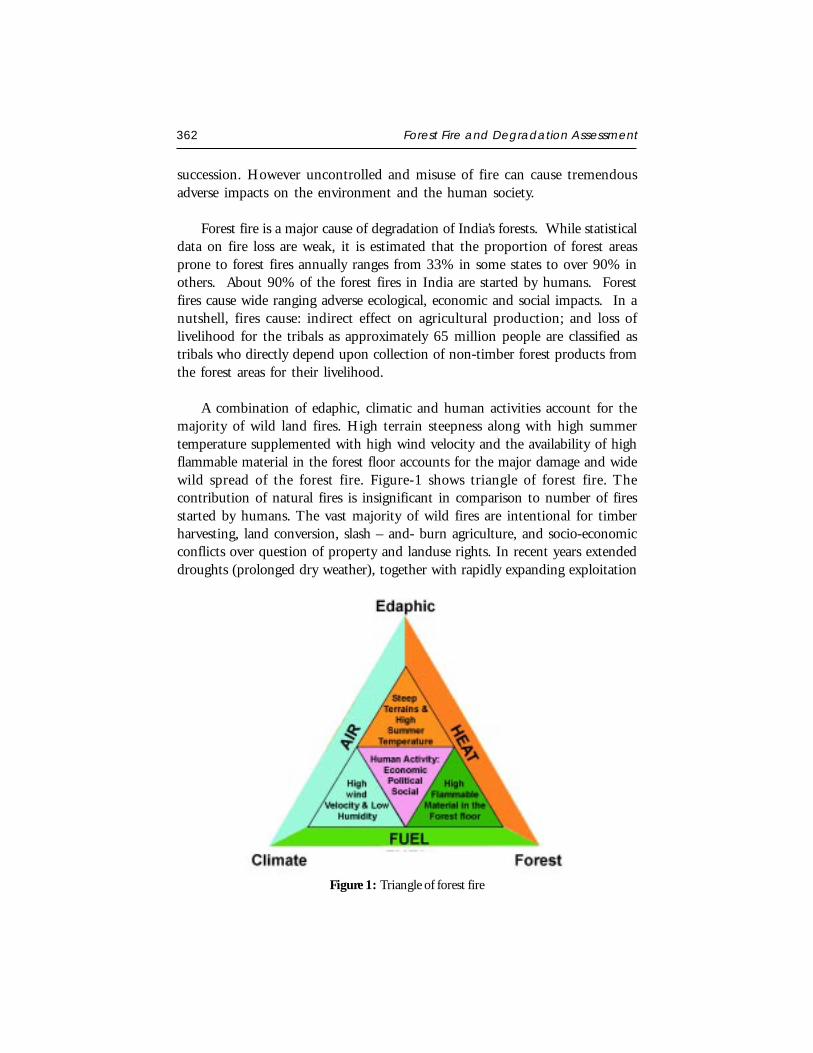
362 Forest Fire and Degradation Assessment
succession. However uncontrolled and misuse of fire can cause tremendousadverse impacts on the environment and the human society.
Forest fire is a major cause of degradation of India’s forests. While statisticaldata on fire loss are weak, it is estimated that the proportion of forest areasprone to forest fires annually ranges from 33% in some states to over 90% inothers. About 90% of the forest fires in India are started by humans. Forestfires cause wide ranging adverse ecological, economic and social impacts. In anutshell, fires cause: indirect effect on agricultural production; and loss oflivelihood for the tribals as approximately 65 million people are classified astribals who directly depend upon collection of non-timber forest products fromthe forest areas for their livelihood.
A combination of edaphic, climatic and human activities account for themajority of wild land fires. High terrain steepness along with high summertemperature supplemented with high wind velocity and the availability of highflammable material in the forest floor accounts for the major damage and widewild spread of the forest fire. Figure-1 shows triangle of forest fire. Thecontribution of natural fires is insignificant in comparison to number of firesstarted by humans. The vast majority of wild fires are intentional for timberharvesting, land conversion, slash – and- burn agriculture, and socio-economicconflicts over question of property and landuse rights. In recent years extendeddroughts (prolonged dry weather), together with rapidly expanding exploitation
Figure 1: Triangle of forest fire
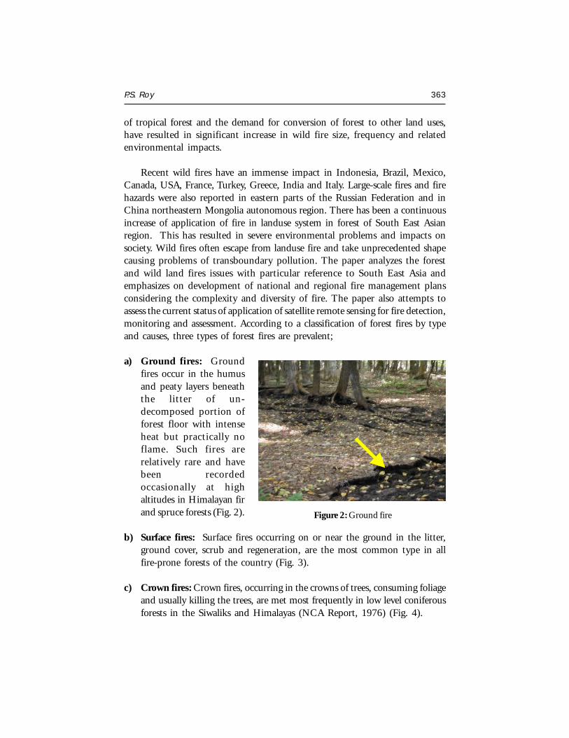
P.S. Roy 363
of tropical forest and the demand for conversion of forest to other land uses,have resulted in significant increase in wild fire size, frequency and relatedenvironmental impacts.
Recent wild fires have an immense impact in Indonesia, Brazil, Mexico,Canada, USA, France, Turkey, Greece, India and Italy. Large-scale fires and firehazards were also reported in eastern parts of the Russian Federation and inChina northeastern Mongolia autonomous region. There has been a continuousincrease of application of fire in landuse system in forest of South East Asianregion. This has resulted in severe environmental problems and impacts onsociety. Wild fires often escape from landuse fire and take unprecedented shapecausing problems of transboundary pollution. The paper analyzes the forestand wild land fires issues with particular reference to South East Asia andemphasizes on development of national and regional fire management plansconsidering the complexity and diversity of fire. The paper also attempts toassess the current status of application of satellite remote sensing for fire detection,monitoring and assessment. According to a classification of forest fires by typeand causes, three types of forest fires are prevalent;
a) Ground fires: Groundfires occur in the humusand peaty layers beneaththe litter of un-decomposed portion offorest floor with intenseheat but practically noflame. Such fires arerelatively rare and havebeen recordedoccasionally at highaltitudes in Himalayan firand spruce forests (Fig. 2).
b) Surface fires: Surface fires occurring on or near the ground in the litter,ground cover, scrub and regeneration, are the most common type in allfire-prone forests of the country (Fig. 3).
c) Crown fires: Crown fires, occurring in the crowns of trees, consuming foliageand usually killing the trees, are met most frequently in low level coniferousforests in the Siwaliks and Himalayas (NCA Report, 1976) (Fig. 4).
Figure 2: Ground fire
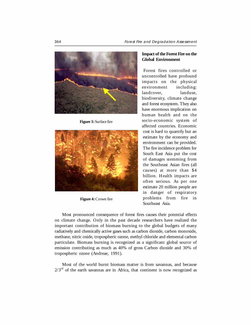
364 Forest Fire and Degradation Assessment
Impact of the Forest Fire on theGlobal Environment
Forest fires controlled oruncontrolled have profoundimpacts on the physicalenvironment including:landcover, landuse,biodiversity, climate changeand forest ecosystem. They alsohave enormous implication onhuman health and on thesocio-economic system ofaffected countries. Economiccost is hard to quantify but anestimate by the economy andenvironment can be provided.The fire incidence problem forSouth East Asia put the costof damages stemming fromthe Southeast Asian fires (allcauses) at more than $4billion. Health impacts areoften serious. As per oneestimate 20 million people arein danger of respiratoryproblems from fire inSoutheast Asia.
Most pronounced consequence of forest fires causes their potential effectson climate change. Only in the past decade researchers have realized theimportant contribution of biomass burning to the global budgets of manyradiatively and chemically active gases such as carbon dioxide, carbon monoxide,methane, nitric oxide, tropospheric ozone, methyl chloride and elemental carbonparticulate. Biomass burning is recognized as a significant global source ofemission contributing as much as 40% of gross Carbon dioxide and 30% oftropospheric ozone (Andreae, 1991).
Most of the world burnt biomass matter is from savannas, and because2/3rd of the earth savannas are in Africa, that continent is now recognized as
Figure 4: Crown fire
Figure 3: Surface fire
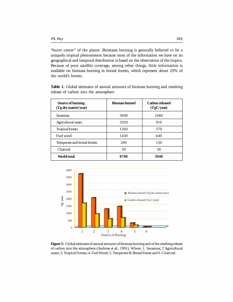
P.S. Roy 365
“burnt center” of the planet. Biomasss burning is generally believed to be auniquely tropical phenomenon because most of the information we have on itsgeographical and temporal distribution is based on the observation of the tropics.Because of poor satellite coverage, among other things, little information isavailable on biomass burning in boreal forests, which represent about 29% ofthe world’s forests.
Table 1. Global estimates of annual amounts of biomass burning and resultingrelease of carbon into the atmosphere
Source of burning Biomass burned Carbon released(Tg dry matter/year) (TgC/year)
Savannas 3690 1660
Agricultural waste 2020 910
Tropical forests 1260 570
Fuel wood 1430 640
Temperate and boreal forests 280 130
Charcoal 20 30
World total 8700 3940
Figure 5: Global estimates of annual amounts of biomass burning and of the resulting releaseof carbon into the atmosphere (Andreae et al., 1991). Where, 1. Savannas; 2 Agriculturalwaste; 3. Tropical Forests; 4. Fuel Wood; 5. Temperate & Boreal Forest and 6. Charcoal.
0
500
1000
1500
2000
2500
3000
3500
4000
Source of Burning
Biomass burned (Tg dry matter/year)
Carbon released (Tg C/year)
1 2 3 4 5 6
Tg
/ yea
r
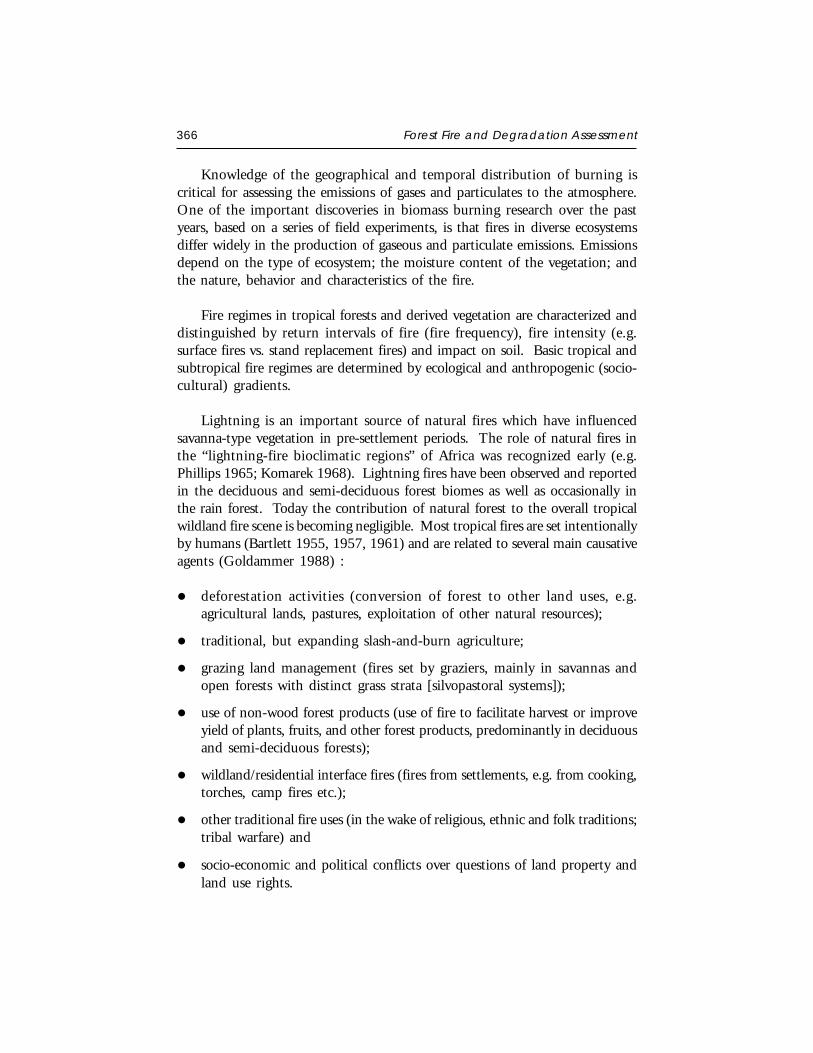
366 Forest Fire and Degradation Assessment
Knowledge of the geographical and temporal distribution of burning iscritical for assessing the emissions of gases and particulates to the atmosphere.One of the important discoveries in biomass burning research over the pastyears, based on a series of field experiments, is that fires in diverse ecosystemsdiffer widely in the production of gaseous and particulate emissions. Emissionsdepend on the type of ecosystem; the moisture content of the vegetation; andthe nature, behavior and characteristics of the fire.
Fire regimes in tropical forests and derived vegetation are characterized anddistinguished by return intervals of fire (fire frequency), fire intensity (e.g.surface fires vs. stand replacement fires) and impact on soil. Basic tropical andsubtropical fire regimes are determined by ecological and anthropogenic (socio-cultural) gradients.
Lightning is an important source of natural fires which have influencedsavanna-type vegetation in pre-settlement periods. The role of natural fires inthe “lightning-fire bioclimatic regions” of Africa was recognized early (e.g.Phillips 1965; Komarek 1968). Lightning fires have been observed and reportedin the deciduous and semi-deciduous forest biomes as well as occasionally inthe rain forest. Today the contribution of natural forest to the overall tropicalwildland fire scene is becoming negligible. Most tropical fires are set intentionallyby humans (Bartlett 1955, 1957, 1961) and are related to several main causativeagents (Goldammer 1988) :
deforestation activities (conversion of forest to other land uses, e.g.agricultural lands, pastures, exploitation of other natural resources);
traditional, but expanding slash-and-burn agriculture;
grazing land management (fires set by graziers, mainly in savannas andopen forests with distinct grass strata [silvopastoral systems]);
use of non-wood forest products (use of fire to facilitate harvest or improveyield of plants, fruits, and other forest products, predominantly in deciduousand semi-deciduous forests);
wildland/residential interface fires (fires from settlements, e.g. from cooking,torches, camp fires etc.);
other traditional fire uses (in the wake of religious, ethnic and folk traditions;tribal warfare) and
socio-economic and political conflicts over questions of land property andland use rights.
P.S. Roy 367
Comparatively little is known empirically about the vegetation fire regimeof Southeast Asia when viewed at larger scales. This is despite the importanceof fire as an agent of regional land cover change and in modifying atmosphericchemistry. Fire is widely used in rice cultivation in Asia where 94 % of theworld’s crop is grown (Nguyen et al., 1994). It also has a high incidence withinforests in tropical Asia (Hao and Liu, 1994) where it is mainly associated withshifting cultivation (McNeely et al., 1991). As with the tropics and the Africantropics, Southeast Asian tropical forests are of considerable ecological andeconomic importance and make up about 20% of the world’s tropical forestresource (after FAO, 1993). Information on biomass burning within the Indo-Malayan region is needed to assist in the modelling of large-scale atmosphericpollution and climate change phenomena and for regional use by landusemanagers, habitat conservationists, and national and regional policy makers.Mainland Southeast Asia is the focus of the Southeast Asian fire, since it ismore strongly seasonal and less humid than many parts of insular South-eastAsia (Nix, 1983) and thus both favour the use of fire as a land managementtool and support more fire-prone ecosystems (54% of forest formations aretropical seasonal forest compared to 4% within insular regions, FAO, 1993).The mainland Southeast Asian product offers an analysis of the spatial andtemporal distribution of vegetation fire in mainland Southeast Asia usingAVHRR 1 km resolution data for the period of single dry season (that chosen isfrom November 1992 to April 1993).
The Socio-Economic and Cultural Background of Forest Fires
While many of the publications cited above contain information on firecauses, there are only few in-depth studies available on the socio-economic andcultural aspects of managing the fire problem. The forest fire managementsystem in Thailand has its strong base on a fire prevention approach which isbeing realized by a close cooperation with the local population (cf. Contributionby S. Akaakara, this volume). The same refers to the IFFM approach in Indonesia(cf. Contribution by H. Abberger, this volume; see also the work of Otsuka[1991] on forest management and farmers in East Kalimantan). A basic studyon the socio-economic and cultural background of forest fires in the pine forestsof the Philippines was conducted in the late 1980s and reveals the usefulnessof such surveys for further management planning (Noble, 1990).
Despite the initial efforts it must be stated that there is a tremendous gapof expertise and available methodologies of socio-economic and culturalapproaches in integrating people into operational fire management systems.
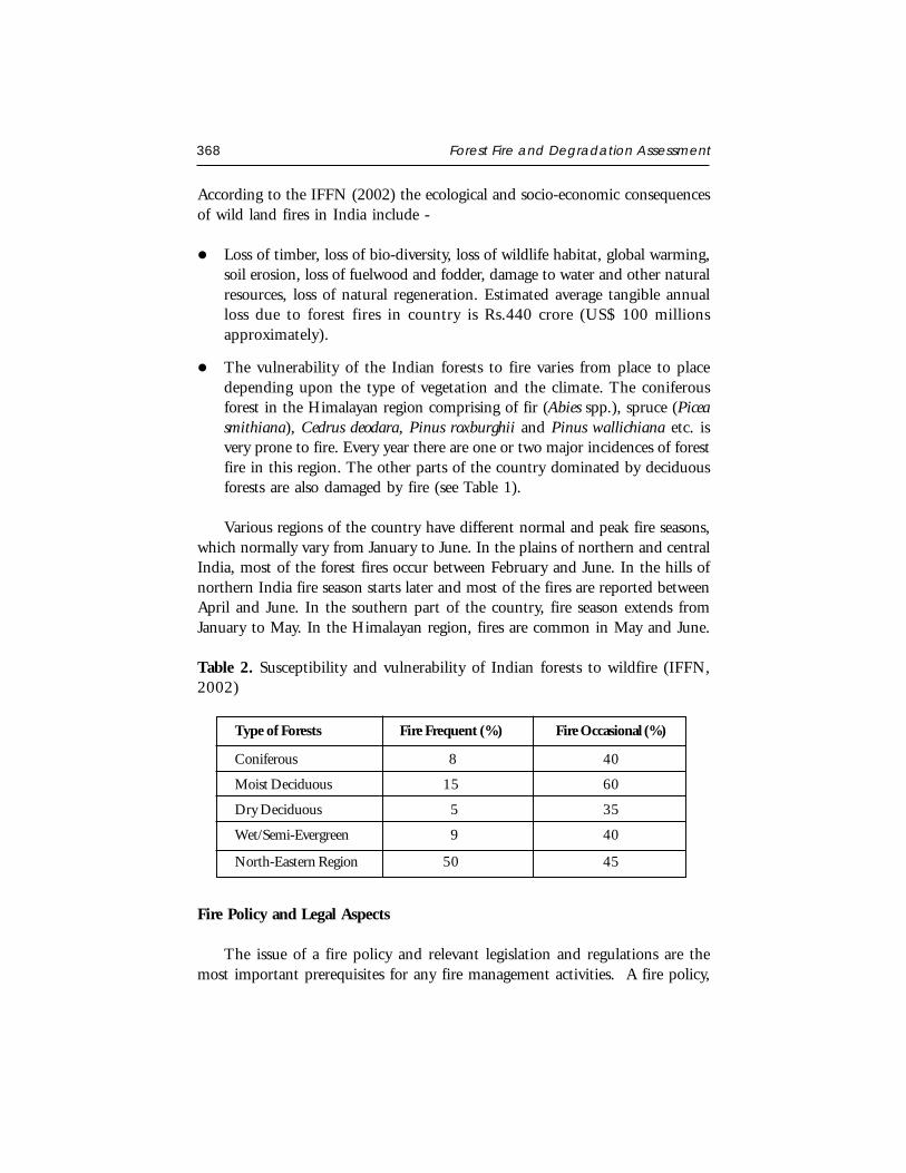
368 Forest Fire and Degradation Assessment
According to the IFFN (2002) the ecological and socio-economic consequencesof wild land fires in India include -
Loss of timber, loss of bio-diversity, loss of wildlife habitat, global warming,soil erosion, loss of fuelwood and fodder, damage to water and other naturalresources, loss of natural regeneration. Estimated average tangible annualloss due to forest fires in country is Rs.440 crore (US$ 100 millionsapproximately).
The vulnerability of the Indian forests to fire varies from place to placedepending upon the type of vegetation and the climate. The coniferousforest in the Himalayan region comprising of fir (Abies spp.), spruce (Piceasmithiana), Cedrus deodara, Pinus roxburghii and Pinus wallichiana etc. isvery prone to fire. Every year there are one or two major incidences of forestfire in this region. The other parts of the country dominated by deciduousforests are also damaged by fire (see Table 1).
Various regions of the country have different normal and peak fire seasons,which normally vary from January to June. In the plains of northern and centralIndia, most of the forest fires occur between February and June. In the hills ofnorthern India fire season starts later and most of the fires are reported betweenApril and June. In the southern part of the country, fire season extends fromJanuary to May. In the Himalayan region, fires are common in May and June.
Table 2. Susceptibility and vulnerability of Indian forests to wildfire (IFFN,2002)
Type of Forests Fire Frequent (%) Fire Occasional (%)
Coniferous 8 40
Moist Deciduous 15 60
Dry Deciduous 5 35
Wet/Semi-Evergreen 9 40
North-Eastern Region 50 45
Fire Policy and Legal Aspects
The issue of a fire policy and relevant legislation and regulations are themost important prerequisites for any fire management activities. A fire policy,

P.S. Roy 369
which would be a basic commitment to the fire problem and the definition ofa national concept of policies to encounter fire-related problems, needs toembrace the following basic considerations (if not at national level, a policymay also be formulated at the regional or district level):
a. A general statement on the role and impacts of fire in the most importantforests and other vegetation of the country (or management unit).
b. A general statement regarding how to counter the negative impacts of fire.
c. Definition of an overall fire management strategy. Definition of firemanagement policy in the various geographic regions in accordance withvegetation type, demographics and land uses.
d. Definition of the role of the population in participating in fire managementactivities, especially in fire prevention.
A variety of legal aspects needs to be considered for the implementation ofa fire policy and for coherent fire management planning, in general e.g. :
a. Clear definition of landownership and availability of a landownershipregister.
b. Development of a landscape plan in which clear definitions are given of theland uses permitted or practiced on a defined area of land.
c. Regulations concerning construction in forests and wildlands, especiallyon burned areas.
d. Clear definition of fire management responsibilities as related to the varioustypes of land ownerships and different tasks in fire management, e.g. fireprevention, fire detection, and fire suppression (including coordinationand cooperation).
e. Rehabilitation of burned lands.
f. Law enforcement.
Regional Co-operation in Forest Fire Management
Beginning in 1992, as a consequence of the regional smog problems causedby land-use fires, member states of the Association of South East Asian Nations(ASEAN) created joint activities to encounter problems arising from
370 Forest Fire and Degradation Assessment
transboundary haze pollution. ASEAN workshops held in Balikpapan (1992)and Kuala Lumpur (1995) summarized the problems and urged appropriateinitiatives. The ASEAN Conference on “Transboundary Pollution and theSustainability of Tropical Forests” is one of the first important steps to materializethe conceptual framework proposed during the past years.
Most important in future regional ASEAN-wide cooperation in firemanagement will be the sharing of resources. The foci will be :
predicting fire hazard and fire effects on ecosystems and atmosphere;
detection, monitoring and evaluating fires; and
sharing fire suppression technologies.
The ASEAN Fire Forum during this meeting will provide importantrecommendations on joint future actions. The ASEAN region will potentiallyserve as a pilot region in which resource sharing will be based on the fact thattwo distinct fire problem seasons exist within the region. While within Indonesiathe fire season is mainly during the months of September to November (southernhemisphere dry season), the fire season in monsoon-influenced SE Asia isbetween January and May. Sharing resources means that hard and softwaretechnologies and required personnel can concentrate on the hemispheric fireproblems, and even costly fire suppression equipment, e.g. airplanes, can beused more economically throughout the whole year.
Forest Degradation & Fire Disasters in India during the Past Few Years
The normal fire season in India is from the month of February to mid June.India witnessed the most severe forest fires in the recent time during the summerof 1995 in the hills of Uttar Pradesh and Himachal Pradesh in the Himalayasin northern part of India. The fires were very severe and attracted the attentionof whole nation. An area of 677, 700 ha was affected by fires. The quantifiabletimber loss was around US$ 45 million. The loss to timber increment, loss ofsoil fertility, soil erosion, loss of employment, drying up of water sources andloss to biodiversity were not calculated by the Committee appointed by theGovernment to enquire into the causes of fires, as these losses are immeasurablebut very significant from the point of view of both economy as well as ecology.The fires in the hills resulted in smoke in the area for quite a few days. Thesmoke haze, however, vanished after the onset of rains. These fires caused changesin the micro-climate of the area in the form of soil moisture balance and increased
P.S. Roy 371
evaporation. Lack of adequate manpower, communication and, water availabilityin the hills helped this fire spread rapidly reaching the crown level. The thicksmoke spread over the sky affecting visibility up to 14,000 feet.
Assessment of Forest Degradation
The statistics on forest fire damage are very poor in the country. In theabsence of proper data, it is difficult to arrive at the accurate losses from theforest fires. Moreover, the losses from fires in respect of changes in biodiversity,carbon sequestration capability, soil moisture and nutrient losses etc are verysignificant from the point of view of ecological stability and environmentalconservation. To a certain extent, the loss due to forest fires can be estimatedbased on the inventories made by the Forest Survey of India (FSI) as reportedin the state of forest report 1995 and subsequent field observations conductedby them. The statistics of losses from forest fires from the various states of theunion is still very sketchy and fragmented. Much of the data available does notreflect the ground situation and is grossly under reported. The total reportedloss from the states of the union is around US$ 7.5 million annually.
The Forest Survey of India data indicate 50% of the forest areas as fireprone. This does not mean that country’s 50% area is affected by fires annually.Very heavy, heavy and frequent forest fire damage are noticed only over 0.8%,0.14% and 5.16% of the forest areas respectively. Thus, only 6.17% of theforests are prone to severe fire damage. In absolute terms, out of the 63 millionha of forests an area of around 3.73 million ha can be presumed to be affectedby fires annually. At this level the annual losses from forest fires in India for theentire country can be moderately estimated at US$ 107 million. This estimatedoes not include the loss suffered in the form of loss of biodiversity, nutrientand soil moisture and other intangible benefits. Based on the UNDP projectevaluation report of 1987, if 40 million ha of forests are saved annually fromforest fires due to implementation of modern forest fire control methods, thenet amount saved at todays’ prices would come to be US$ 6.8 million.
Remote Sensing & Geographic Information System
Satellite observations providing a global survey of the composition of biomassburning plumes and their dispersal in the global atmosphere will becomeavailable by the middle to late 1990s and will be an important contribution tothis task. Global mapping of CO and O3 columns can be achieved by theGlobal Ozone Monitoring Experiment (GOME) and Scanning Imaging
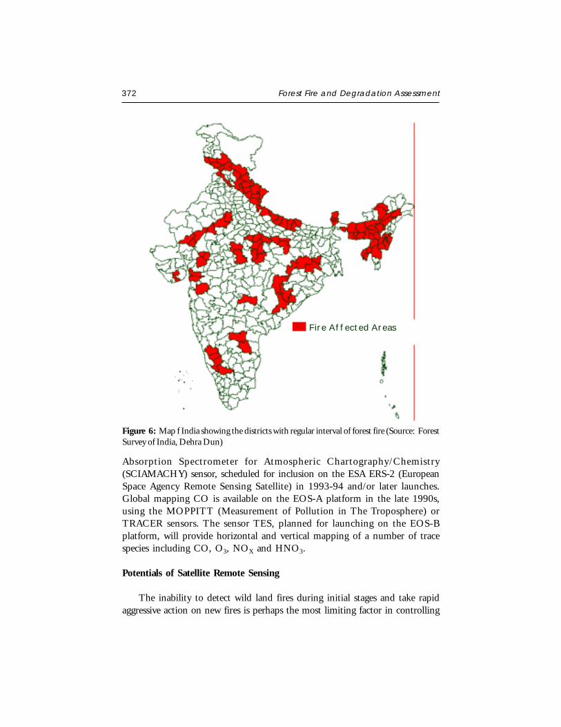
372 Forest Fire and Degradation Assessment
Absorption Spectrometer for Atmospheric Chartography/Chemistry(SCIAMACHY) sensor, scheduled for inclusion on the ESA ERS-2 (EuropeanSpace Agency Remote Sensing Satellite) in 1993-94 and/or later launches.Global mapping CO is available on the EOS-A platform in the late 1990s,using the MOPPITT (Measurement of Pollution in The Troposphere) orTRACER sensors. The sensor TES, planned for launching on the EOS-Bplatform, will provide horizontal and vertical mapping of a number of tracespecies including CO, O3, NOX and HNO3.
Potentials of Satellite Remote Sensing
The inability to detect wild land fires during initial stages and take rapidaggressive action on new fires is perhaps the most limiting factor in controlling
Fire Affected Areas
Figure 6: Map f India showing the districts with regular interval of forest fire (Source: ForestSurvey of India, Dehra Dun)
P.S. Roy 373
such wild land fires. This is especially true for fires in areas with limited access.Providing an effective response to wildland fires requires four stages of analysisand assessment:
Determining fire potential risk
Detecting fire starts
Monitoring active fires
Conducting post-fire degradation assessment
The technological advancement in space remote sensing has been widelyexperimented in last three decades to obtain the desired information.
Fire Potential
Fire potential depends on the amount of dead and live vegetation andmoisture contents in each. The amount of dead and live vegetation is estimatedfrom a high quality landcover map derived from (ideally) a high resolutionsensor, such as the IRS, Landsat TM or SPOT multispectral scanner or fromlower resolution sensor such as NOAA-AVHRR or NASA Moderate ResolutionImaging Spectrometer (MODIS). These satellites can be used to monitor changesin the vegetation vigor, which is correlated with the moisture of the livevegetation. The moisture in the dead vegetation is estimated from knowledgeof local weather conditions. Thus, a baseline land cover map and immediateestimate of vegetation condition are needed.
The research project FIRE in global Resource and Environmental monitoring(FIRE) was initiated in 1994 by the Monitoring of Tropical Vegetation unit(MTV) of the Commission of the European Union Joint Research Centre inorder to address such issues. A key objective of this initiative was thedocumentation of vegetation fire patterns for the entire globe and the analysesof such patterns in relation to land use/land cover dynamics in tropical andinter-tropical regions. Obviously, such vegetation fires represent only part ofthe overall biomass burning activity, which also includes the burning of domesticfuels, occurring at the surface of the Earth. Due to both the characteristics ofthe phenomenon and to the multiscale objective, the fire monitoring systemunder development in the MTV Unit relies on remote sensing techniques asthe main source of information. This is the case since earth observation fromspace provides systematic and consistent measurements of a series of parameters
374 Forest Fire and Degradation Assessment
related to fire and fire impacts, and, consequently, is an ideal medium for thestudy of vegetation fire. The AVHRR on the NOAA satellites is the main sourceof data for the studies done by the FIRE project. For the 5 km GAC (GlobalArea Coverage) data, historical archives exist that extend back to 1981 andconsist of daily images covering the entire globe. More limited data sets, fromthe same AVHRR sensor but at 1 km resolution also exist at global, continentaland regional level. A mobile AVHRR data receiving station is also used by theFIRE project.
Fire Detection
Satellite-borne sensors can detect fires in the visible, thermal and mid-infrared bands. Active fires can be detected by their thermal or mid-infraredsignature during the day or by the light from the fires at night. For theirdetection the sensors must also provide frequent overflights, and the data fromthe overflights must be available fast. Satellite systems that have been evaluatedfor fire detection include AVHRR, which has a thermal sensor and makes dailyoverflights, the Defense Meteorological Satellite Program (DMSP) OpticalLinescan System (OLS) sensor, which makes daily overflights and routinelycollects visible images during its nighttime pass, and the NOAA GeostationaryOperational Environmental Satellite (GOES) sensor, which provides visibleand thermal images every 15 minutes over the United States and every 30minutes elsewhere. Therefore AVHRR has been used most extensively fordetecting and monitoring wildfires.
Fire Monitoring
Fire monitoring differs from fire detection in timing and emphasis ratherthan in the methods used to process the satellite image information. Satellitesensors typically provide coarse resolution fire maps which show the generallocation and extent of wildland fires. Detailed fire suppression mapping requiresthe use of higher resolution airborne thermal infrared sensors to accuratelymap small fire hot-spots and active fire perimeters. Higher-resolution fire mapsare needed to deploy fire suppression crews and aerial water or retardant drops.
Fire Assessment
Once fires are extinguished, a combination of low resolution images(AVHRR) and higher-resolution images (SPOT, Landsat and Radar) can beused to assess the extent and impact of the fire. Radar has proved effective in

P.S. Roy 375
monitoring and assessing the extent and severity of fire scars in the boreal forests(Kasischke et al., 1994), for quantifying biomass regeneration in tropical forests(Luckman et al., 1997) and for modeling ecosystem recovery in Mediterraneanclimates (Vietma et al., 1997). Low resolution visible and infrared sensors suchas AVHRR have proved useful for automated fire mapping (Fernandes et al.,1997) and for evaluating the impact of fire on long-term land cover change(Ehrlich et al., 1997). Multi-resolution studies incorporating both AVHRRand Landsat images reveal the scale-related influences of analyzing post-firevegetation regeneration (Steyaert et al., 1997).
Information related to new fire scars and vegetation succession within thescars can be used to update the baseline vegetation map used for fire prediction.Continued monitoring of the fire scars provides extensive information on landcover transitions involving changes in productivity and biodiversity, which inturn influence fire potential. Knowledge of the extent and intensity of fire scarsprovides important information for the rehabilitation of the burn areas.
Globally no reliable statistics about the exact location and annual areasburnt by forest fire are available. The information required and what can beachieved using Remote Sensing data are presented as Table 3.
Table 3. Forest Fire Assessment
Class of Information Type of Information
a) alpha type Fire : start and end dates, location, size and cause
b) beta type Fuels biome classification and fuel loading forestinventory (number), age class, size class
c) gamma type Fire characterisation (crown, surface etc.), fuelconsumption and structural involvement (wildlandurban interface)
d) delta type Number of fires, areas burnt (by forest type), cause offires (number)
e) epsilon type Gas and aerosol emission data
f) eta type Total expenditure of fire programme, total firesuppression costs and total direct losses of merchantabletimber, structure losses
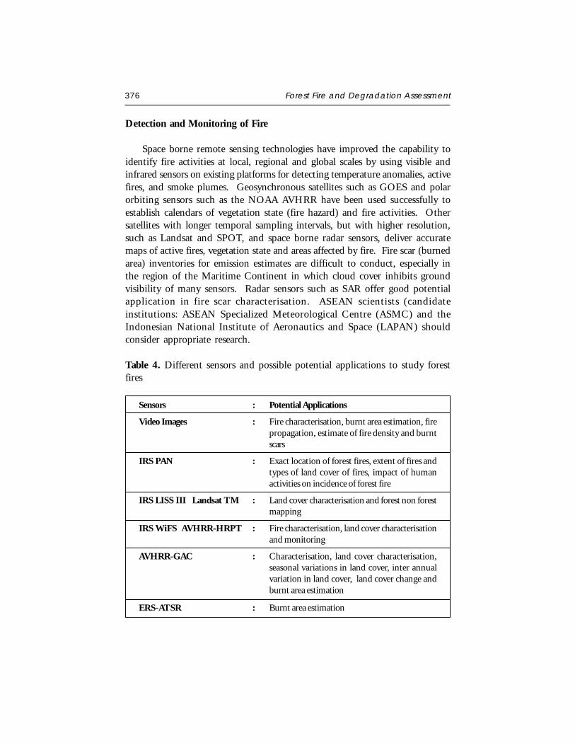
376 Forest Fire and Degradation Assessment
Detection and Monitoring of Fire
Space borne remote sensing technologies have improved the capability toidentify fire activities at local, regional and global scales by using visible andinfrared sensors on existing platforms for detecting temperature anomalies, activefires, and smoke plumes. Geosynchronous satellites such as GOES and polarorbiting sensors such as the NOAA AVHRR have been used successfully toestablish calendars of vegetation state (fire hazard) and fire activities. Othersatellites with longer temporal sampling intervals, but with higher resolution,such as Landsat and SPOT, and space borne radar sensors, deliver accuratemaps of active fires, vegetation state and areas affected by fire. Fire scar (burnedarea) inventories for emission estimates are difficult to conduct, especially inthe region of the Maritime Continent in which cloud cover inhibits groundvisibility of many sensors. Radar sensors such as SAR offer good potentialapplication in fire scar characterisation. ASEAN scientists (candidateinstitutions: ASEAN Specialized Meteorological Centre (ASMC) and theIndonesian National Institute of Aeronautics and Space (LAPAN) shouldconsider appropriate research.
Table 4. Different sensors and possible potential applications to study forestfires
Sensors : Potential Applications
Video Images : Fire characterisation, burnt area estimation, firepropagation, estimate of fire density and burntscars
IRS PAN : Exact location of forest fires, extent of fires andtypes of land cover of fires, impact of humanactivities on incidence of forest fire
IRS LISS III Landsat TM : Land cover characterisation and forest non forestmapping
IRS WiFS AVHRR-HRPT : Fire characterisation, land cover characterisationand monitoring
AVHRR-GAC : Characterisation, land cover characterisation,seasonal variations in land cover, inter annualvariation in land cover, land cover change andburnt area estimation
ERS-ATSR : Burnt area estimation
P.S. Roy 377
The fire episode of 1997 in Indonesia has clearly demonstrated that the“hot spot” information generated by the NOAA AVHRR is of limited value.New sensors are currently developed which are specifically aimed to satisfy thedemands of the fire science and management community, e.g., the BIRD satelliteproject of the Deutsche Forschungsanstaltfur Luft- und Raumfahrt (DLR) (witha two-channel infrared sensor system in combination with a wide-angleoptoelectronic stereo scanner) and the envisaged fire sensor component FOCISon the International Space Station (Briess et al., 1997; DLR 1997). Indonesia’sMinistry for Research and Technology (BPPT) is interested to collaborate withthe DLR in testing and validating the BIRD satellite.
Fire Weather and Fire Danger Forecasts
Weather forecasts at short to extended time ranges and global to regionalspace scales can be utilized for wildland fire management, e.g. the recent proposalby the US National Centre for Environmental Prediction (NCEP). TheNormalized Difference Vegetation Index (NDVI) has been successfully usedfor estimating fire danger. A recent (not yet published, 1997) report of theIDNDR (IDNDR 1997) gives an overview on a series of candidate systems forearly warning of fire precursors which should investigated by Indonesianscientists.
The proposed Canadian project “Fire Danger Rating System for Indonesia: An Adaptation of the Canadian Fire Behavior Prediction System” will be animportant contribution towards improving the basic knowledge on the weather-fuel-fire/fire behaviour relationships.
The fire danger rating systems which are already in use in some parts ofIndonesia (IFFM-GTZ), however, may be more readily available to produce aregional early warning system within a relatively short time period of a fewmonths. The ministry of Environment of Singapore has indicated interest totest the system at ASEAN level.
The ASEAN Fire Weather Information System (ASFWIS) is a co-operationbetween ASEAN and the Canadian Forest Service. It provides maps describingthe current fire weather situation in South East Asia. This system is basedupon the Canadian Forest Fire Danger Rating System (CFFDRS) (for furtherinformation to the CFFDRS refers to ASFWIS). Studies have shown that theCFFDRS is applicable outside of Canada. Currently it is also used in a modifiedform in New Zealand. In New Zealand the Fire Weather Indices Fine Fuel
378 Forest Fire and Degradation Assessment
Moisture Code (FFMC) and the Initial Spread Index (ISI) represent the firedanger in the scrublands. The Duff Moisture Code (DMC) is also applicablein South East Asia, because it potentially describes the moisture state of theupper peat layers in peat and peat swamp forests. All three parameters mayserve as a suitable indicator of forest fire danger in South East Asia.
CASE STUDIES
Forest Fire Assessment
Forest Fire Prone Area Mapping – A Case Study in GIR-Protected Area
The following study had been carried out in GIR forest which is located inthe Saurashtra Peninsula of Gujarat. It is the largest biologically intact contourstract of forest and the only abide of the Asiatic Lion in the world. The mainobjective of the study is to design, develop and demonstrate RS/GIS basedapproach in order to prepare region/type level fire danger rating system takinginto consideration risk, hazard, meteorological parameters and humaninterventions and also to prepare forest fire risk area/disaster map for GIR forestGujarat. Two types of data are used in the study i.e. spatial and non spatial.Spatial data mainly includes Remote Sensing data, forest block, compartmentboundaries, road/railway network and the most important existing water bodiesin that area where the non-spatial data pertains to meteorological data ontemperature, relative boundary, rainfall, wind, socio-economic data.
The methodology adopted was visual, digital and hybrid method for RemoteSensing data analysis. IRS 1C/1D LISS III FCC’s were used for visualinterpretation for classification of vegetation in the entire GIR-PA region. Toidentify fire scars digital data of IRS 1C/1D WiFS had been used. WiFS datahad also been used to delineate water bodies and fire scars. The parametersused for modelling the fire risk zone were –
Fire occurrence maps for three or more seasons
Classified vegetation map (two seasons)
Road network (Proximity analysis)
Maximum temperature
Relative humidity
P.S. Roy 379
Rainfall data
Forest block compartments
Rivers, streams and water bodies
Settlements location map (Proximity analysis)
All these parameters have direct/indirect influence on the occurrence of fireand were integrated using GIS and a multi parametric weighted index modelhas been adopted to derive the ‘fire-risk’ zone map. It is classified into 6 riskzones. It was observed that very high and high zones are mostly at the fringe ofthe protected area or within 100 m of the roads passing through the regionwith temperature above 40oC and humidity less than 35%. Apart from humaninterference the analysis has shown that vegetation type and meteorologicalparameters have vital importance for hazard zonation.
Spatial Modelling Techniques for Forest Fire Risk Assessments
The study attempted to give insight in the use of RS and GIS for firemanagement. Spatial modelling and analysis have been done in GIS environmentfor identification of areas prone to fire risk and subsequently response routeswere suggested for extinguishing forest fires (Jain et al., 1996 and Porwal et al.,1997). Some of the necessary components contributing to the fire behaviourviz., fuel (vegetation types), topography (slope and aspect etc.) and the causesof fire (i.e., roads and settlements) have been given due weightages.
The study has been done in part of Rajaji National Parks covering an areaof approximately 115 km2. The topography is variable within the altituderanging between 300-700 m above msl. The climate is subtropical type withthe temperature varying from 13.1oC in January to 38.9oC in May & June.The area is dominated by moist Siwalik sal forest, moist mixed deciduous forest,dry mixed deciduous forest, chirpine and shrubs.
Landsat TM false colour composite (FCC) and SPOT images on 1:50,000scale have been visually interpreted to obtain primary map layers viz. Forestcover type map, density map etc. The contour map, road network settlementetc. have been obtained from Survey of India toposheets. This spatial data inthe form of map was digitized and transformed in machine-readable form forintegration of thematic information. However, before their integration (Fig. 7)these were converted into index map viz., fuel type index maps from forest
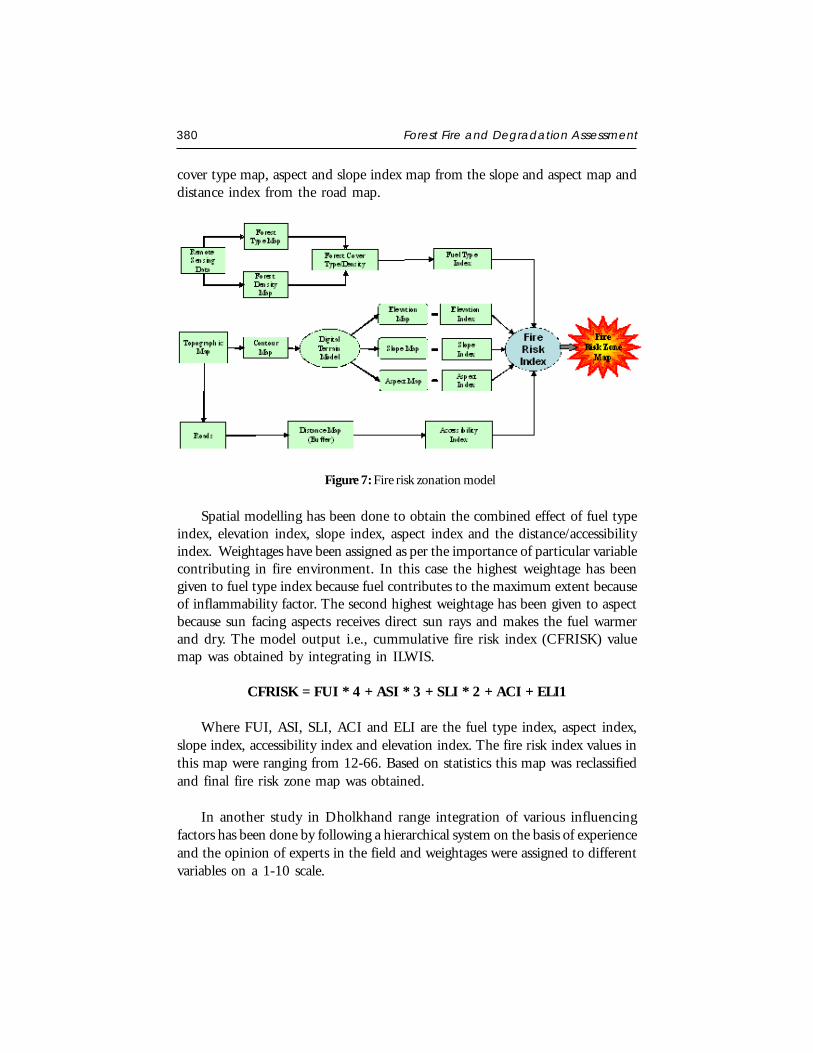
380 Forest Fire and Degradation Assessment
cover type map, aspect and slope index map from the slope and aspect map anddistance index from the road map.
Figure 7: Fire risk zonation model
Spatial modelling has been done to obtain the combined effect of fuel typeindex, elevation index, slope index, aspect index and the distance/accessibilityindex. Weightages have been assigned as per the importance of particular variablecontributing in fire environment. In this case the highest weightage has beengiven to fuel type index because fuel contributes to the maximum extent becauseof inflammability factor. The second highest weightage has been given to aspectbecause sun facing aspects receives direct sun rays and makes the fuel warmerand dry. The model output i.e., cummulative fire risk index (CFRISK) valuemap was obtained by integrating in ILWIS.
CFRISK = FUI * 4 + ASI * 3 + SLI * 2 + ACI + ELI1
Where FUI, ASI, SLI, ACI and ELI are the fuel type index, aspect index,slope index, accessibility index and elevation index. The fire risk index values inthis map were ranging from 12-66. Based on statistics this map was reclassifiedand final fire risk zone map was obtained.
In another study in Dholkhand range integration of various influencingfactors has been done by following a hierarchical system on the basis of experienceand the opinion of experts in the field and weightages were assigned to differentvariables on a 1-10 scale.
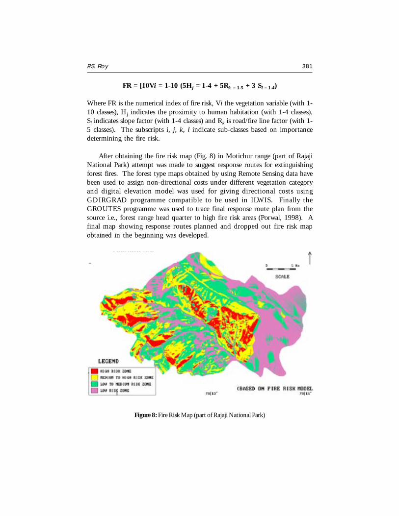
P.S. Roy 381
FR = [10Vi = 1-10 (5Hj = 1-4 + 5Rk = 1-5 + 3 Sl = 1-4)
Where FR is the numerical index of fire risk, Vi the vegetation variable (with 1-10 classes), Hj indicates the proximity to human habitation (with 1-4 classes),Sl indicates slope factor (with 1-4 classes) and Rk is road/fire line factor (with 1-5 classes). The subscripts i, j, k, l indicate sub-classes based on importancedetermining the fire risk.
After obtaining the fire risk map (Fig. 8) in Motichur range (part of RajajiNational Park) attempt was made to suggest response routes for extinguishingforest fires. The forest type maps obtained by using Remote Sensing data havebeen used to assign non-directional costs under different vegetation categoryand digital elevation model was used for giving directional costs usingGDIRGRAD programme compatible to be used in ILWIS. Finally theGROUTES programme was used to trace final response route plan from thesource i.e., forest range head quarter to high fire risk areas (Porwal, 1998). Afinal map showing response routes planned and dropped out fire risk mapobtained in the beginning was developed.
Figure 8: Fire Risk Map (part of Rajaji National Park)
382 Forest Fire and Degradation Assessment
Forest fires cause significant damage to the forest ecosystem. In CentralHimalayan region forest fires occur between April to June annually when theweather is hot and dry. Usually the south facing slopes are prone to fire due todirect sun insulation and inflammable litters of pine and dry deciduous treesat the forest floor. The presence of habitation, roads, footpaths etc., and theirdistance from such sites indicate an additional yardstick for the occurrence offorest fires. Extensive forest area during summer of 1995 in the Western andCentral Himalaya drew wide attention of the forest managers andenvironmentalists. This study attempts to provide estimates about forest firedamaged areas using digital satellite remote sensing data in the Tehri district ofGarhwal Himalaya (Pant et al., 1996).
The study area is characterized by hilly and mountainous terrain supportingvaried forest types and composition controlled by altitude, variety of land use/land cover types along with perpetual snow cover on the mountain peaks. Pineis the dominant forest type and is most susceptible to fire almost every yearparticularly near habitation.
The Indian Remote Sensing Satellite-1B, LISS-II (IRS-B, LISS-II) data ofpre-fire and post fire period (1993-95) were studied and analysed digitally inthe IBM RS/6000, EASI/PACE computer system. The supervised per pixelclassification and digital enhancement approaches have been used to identifythe forest fire affected areas along with other cover types. Prior to this digitalgeometric correction of satellite images have been done using 1:250,000 scaleSurvey of India topographical sheets and both the images were masked withrespect to district boundary. Digital enhancement techniques facilitated tochoose correct training sets for supervised classification technique using maximumlikelihood classifier. The training sets were assigned based on the ground truthinformation collected from fire burnt areas and surrounding cover types. Outof the various enhancement techniques the best result has been obtained bymaking the colour composite image of IR, NDVI and intensity under equalstretching.
The total area affected under forest fire has been estimated as 910.01 km2
or 20.58% of total geographical area of 4421.26 km2. This includes forestburnt area as 168.88 km2 or 3.38% of total geographical area, partially burntforest area (area under active fire) as 473.69 km2 or 10.71% of total geographicalarea and the partially burnt fallow land/grassland/scrub land as 267.44 km2 or6.05%. The forested area identified under smoke plumes has been estimated
P.S. Roy 383
as 130.96 km2 or 2.96% of total forests area. The overall accuracy ofclassification has been assessed as 88%.
FOREST DEGRADATION ASSESSMENT
Deforestation Monitoring
The pressure on forests is greatest in the developing countries. The primarycauses of deforestation are encroachment of forest area for agricultural productionand exploitation of forest cover for meeting housing and industrial needs.Deforestation leads to an increase in the loading of CO2 in the atmosphere.Increased albedo and change in aerodynamic roughness over deforested areasalter the energy balance bearing implications on atmospheric circulation patternsand rainfall statistics. Deforestation leads to soil erosion and gradual loss ofbiodiversity.
The amount of vegetation loss/deforestation due to encroachment can beestimated by the use of remote sensing technique. The impact of slash andburn during and after the ‘jhumming’ (slash and burn agriculture) operationsis clearly visible from remote sensing imageries. The representative relationshipbetween the population density and the percent of forest cover providesinformation about the rate of deforestation and thereby helps in formulatingthe mitigation plan. Utilization of remote sensing tool for stock mapping andgrowing stock estimation for forest management improves reliability. Assam iswell known for its large forest tracts. The recorded forest area in Assam is 39.15%of the geographical area. These forests are repositories of a rich biological diversity.At the same point there is tremendous pressure on these forest lands. There hasbeen an overall decrease of 1,031 sq. km of dense forest from 1997 to 1999 inAssam. This decrease is more pronounced in the Brahmaputra valley in theareas like Sonitpur and others. This study was undertaken after large-scaledeforestation was observed in above district by IIRS team of scientists workingin Arunachal Pradesh. The objective was to assess the large-scale deforestationand loss in biodiversity.
This study covers the entire Sonitpur district (5,103 km2) located in upperAssam valley. Land use within the area is divided primarily among tropicalsemi-evergreen forest, moist deciduous forest, riverain forest, pasture land,agriculture and tea gardens. Good quality Landsat-TM and IRS-1C LISS-IIIfalse colour composites of dry season pertaining to 1994, 1999 and 2001 periodswere used to monitor the loss of biodiversity. All scenes were radiometrically
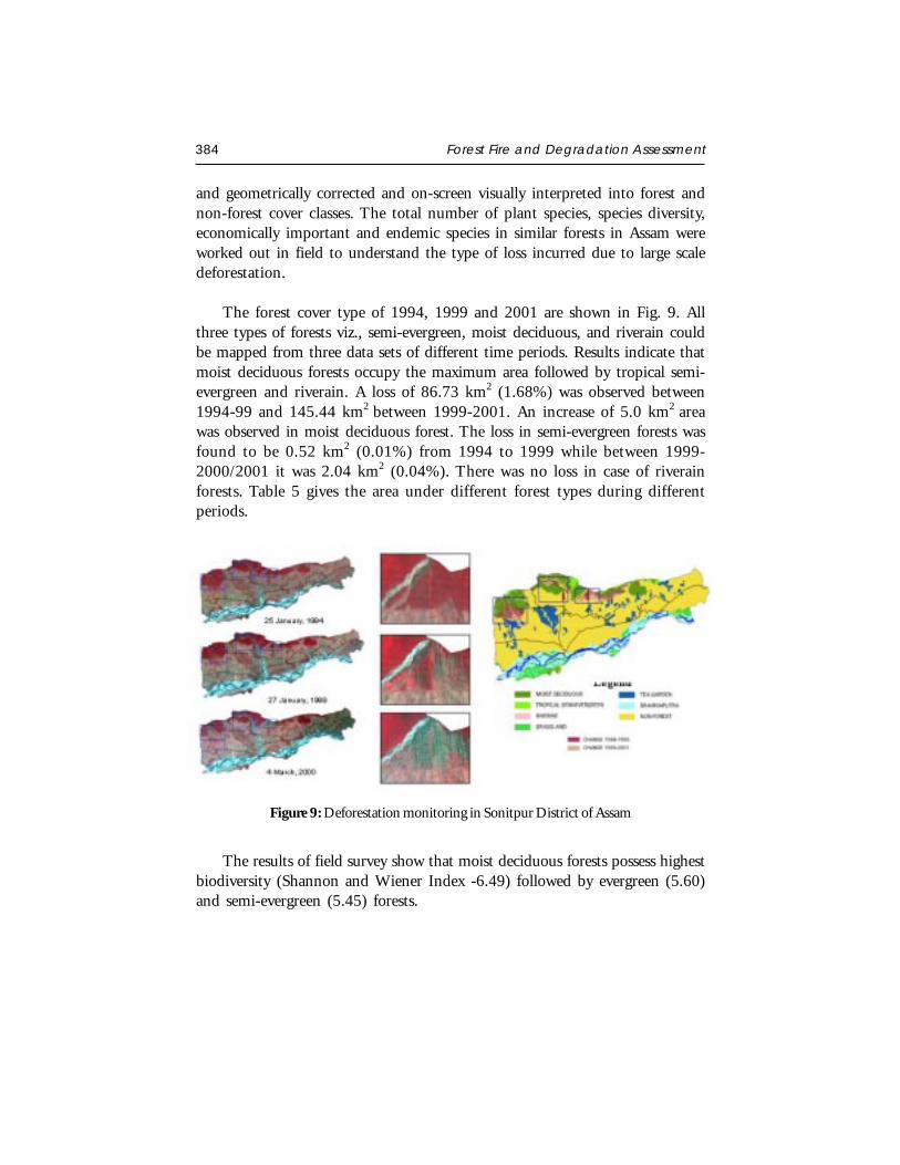
384 Forest Fire and Degradation Assessment
and geometrically corrected and on-screen visually interpreted into forest andnon-forest cover classes. The total number of plant species, species diversity,economically important and endemic species in similar forests in Assam wereworked out in field to understand the type of loss incurred due to large scaledeforestation.
The forest cover type of 1994, 1999 and 2001 are shown in Fig. 9. Allthree types of forests viz., semi-evergreen, moist deciduous, and riverain couldbe mapped from three data sets of different time periods. Results indicate thatmoist deciduous forests occupy the maximum area followed by tropical semi-evergreen and riverain. A loss of 86.73 km2 (1.68%) was observed between1994-99 and 145.44 km2 between 1999-2001. An increase of 5.0 km2 areawas observed in moist deciduous forest. The loss in semi-evergreen forests wasfound to be 0.52 km2 (0.01%) from 1994 to 1999 while between 1999-2000/2001 it was 2.04 km2 (0.04%). There was no loss in case of riverainforests. Table 5 gives the area under different forest types during differentperiods.
Figure 9: Deforestation monitoring in Sonitpur District of Assam
The results of field survey show that moist deciduous forests possess highestbiodiversity (Shannon and Wiener Index -6.49) followed by evergreen (5.60)and semi-evergreen (5.45) forests.
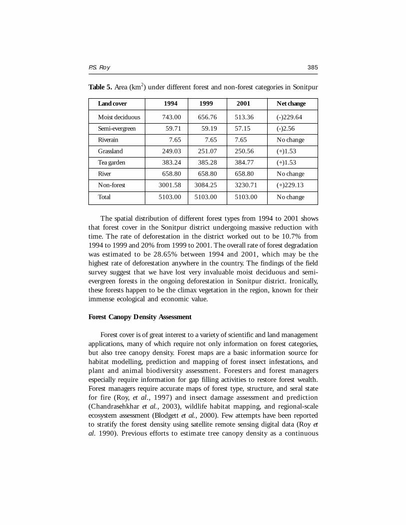
P.S. Roy 385
Table 5. Area (km2) under different forest and non-forest categories in Sonitpur
Land cover 1994 1999 2001 Net change
Moist deciduous 743.00 656.76 513.36 (-)229.64
Semi-evergreen 59.71 59.19 57.15 (-)2.56
Riverain 7.65 7.65 7.65 No change
Grassland 249.03 251.07 250.56 (+)1.53
Tea garden 383.24 385.28 384.77 (+)1.53
River 658.80 658.80 658.80 No change
Non-forest 3001.58 3084.25 3230.71 (+)229.13
Total 5103.00 5103.00 5103.00 No change
The spatial distribution of different forest types from 1994 to 2001 showsthat forest cover in the Sonitpur district undergoing massive reduction withtime. The rate of deforestation in the district worked out to be 10.7% from1994 to 1999 and 20% from 1999 to 2001. The overall rate of forest degradationwas estimated to be 28.65% between 1994 and 2001, which may be thehighest rate of deforestation anywhere in the country. The findings of the fieldsurvey suggest that we have lost very invaluable moist deciduous and semi-evergreen forests in the ongoing deforestation in Sonitpur district. Ironically,these forests happen to be the climax vegetation in the region, known for theirimmense ecological and economic value.
Forest Canopy Density Assessment
Forest cover is of great interest to a variety of scientific and land managementapplications, many of which require not only information on forest categories,but also tree canopy density. Forest maps are a basic information source forhabitat modelling, prediction and mapping of forest insect infestations, andplant and animal biodiversity assessment. Foresters and forest managersespecially require information for gap filling activities to restore forest wealth.Forest managers require accurate maps of forest type, structure, and seral statefor fire (Roy, et al., 1997) and insect damage assessment and prediction(Chandrasehkhar et al., 2003), wildlife habitat mapping, and regional-scaleecosystem assessment (Blodgett et al., 2000). Few attempts have been reportedto stratify the forest density using satellite remote sensing digital data (Roy etal. 1990). Previous efforts to estimate tree canopy density as a continuous
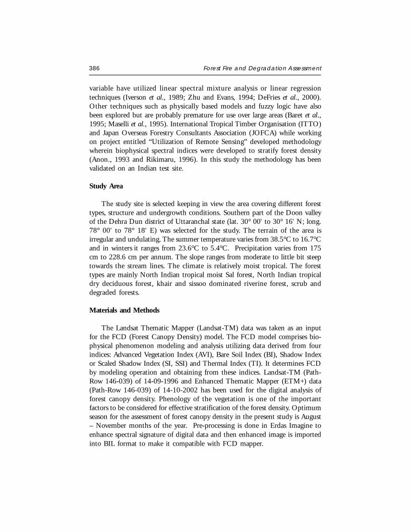
386 Forest Fire and Degradation Assessment
variable have utilized linear spectral mixture analysis or linear regressiontechniques (Iverson et al., 1989; Zhu and Evans, 1994; DeFries et al., 2000).Other techniques such as physically based models and fuzzy logic have alsobeen explored but are probably premature for use over large areas (Baret et al.,1995; Maselli et al., 1995). International Tropical Timber Organisation (ITTO)and Japan Overseas Forestry Consultants Association (JOFCA) while workingon project entitled “Utilization of Remote Sensing” developed methodologywherein biophysical spectral indices were developed to stratify forest density(Anon., 1993 and Rikimaru, 1996). In this study the methodology has beenvalidated on an Indian test site.
Study Area
The study site is selected keeping in view the area covering different foresttypes, structure and undergrowth conditions. Southern part of the Doon valleyof the Dehra Dun district of Uttaranchal state (lat. 30° 00' to 30° 16' N; long.78° 00' to 78° 18' E) was selected for the study. The terrain of the area isirregular and undulating. The summer temperature varies from 38.5°C to 16.7°Cand in winters it ranges from 23.6°C to 5.4°C. Precipitation varies from 175cm to 228.6 cm per annum. The slope ranges from moderate to little bit steeptowards the stream lines. The climate is relatively moist tropical. The foresttypes are mainly North Indian tropical moist Sal forest, North Indian tropicaldry deciduous forest, khair and sissoo dominated riverine forest, scrub anddegraded forests.
Materials and Methods
The Landsat Thematic Mapper (Landsat-TM) data was taken as an inputfor the FCD (Forest Canopy Density) model. The FCD model comprises bio-physical phenomenon modeling and analysis utilizing data derived from fourindices: Advanced Vegetation Index (AVI), Bare Soil Index (BI), Shadow Indexor Scaled Shadow Index (SI, SSI) and Thermal Index (TI). It determines FCDby modeling operation and obtaining from these indices. Landsat-TM (Path-Row 146-039) of 14-09-1996 and Enhanced Thematic Mapper (ETM+) data(Path-Row 146-039) of 14-10-2002 has been used for the digital analysis offorest canopy density. Phenology of the vegetation is one of the importantfactors to be considered for effective stratification of the forest density. Optimumseason for the assessment of forest canopy density in the present study is August– November months of the year. Pre-processing is done in Erdas Imagine toenhance spectral signature of digital data and then enhanced image is importedinto BIL format to make it compatible with FCD mapper.
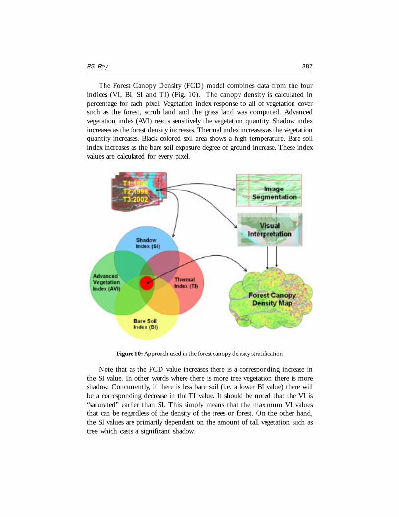
P.S. Roy 387
The Forest Canopy Density (FCD) model combines data from the fourindices (VI, BI, SI and TI) (Fig. 10). The canopy density is calculated inpercentage for each pixel. Vegetation index response to all of vegetation coversuch as the forest, scrub land and the grass land was computed. Advancedvegetation index (AVI) reacts sensitively the vegetation quantity. Shadow indexincreases as the forest density increases. Thermal index increases as the vegetationquantity increases. Black colored soil area shows a high temperature. Bare soilindex increases as the bare soil exposure degree of ground increase. These indexvalues are calculated for every pixel.
Figure 10: Approach used in the forest canopy density stratification
Note that as the FCD value increases there is a corresponding increase inthe SI value. In other words where there is more tree vegetation there is moreshadow. Concurrently, if there is less bare soil (i.e. a lower BI value) there willbe a corresponding decrease in the TI value. It should be noted that the VI is“saturated” earlier than SI. This simply means that the maximum VI valuesthat can be regardless of the density of the trees or forest. On the other hand,the SI values are primarily dependent on the amount of tall vegetation such astree which casts a significant shadow.

388 Forest Fire and Degradation Assessment
Vegetation Density is calculated using vegetation index and bare soil indexas a prime inputs. It is a pre-processing method which uses principal componentanalysis. Because essentially, VI and BI have high negative correlation. Afterthat, set the scaling of zero percent point and a hundred percent point. Theshadow index (SI) is a relative value. Its normalized value can be utilized forcalculation with other parameters.
The SSI was developed in order to integrate VI values and SI values. Inareas where the SSI value is zero, this corresponds with forests that have thelowest shadow value (i.e. 0%). Areas where the SSI value is 100, correspondwith forests that have the highest possible shadow value (i.e.100%). SSI isobtained by linear transformation of SI. With development of SSI one can nowclearly differentiate between vegetation in the canopy and vegetation on theground. This constitutes one of the major advantages of the new methods. Itsignificantly improves the capability to provide more accurate results from dataanalysis than was possible in the past. Integration of VD and SSI meanstransformation for forest canopy density value. Both parameters have dimensionand percentage scale unit of density. It is possible to synthesize both theseindices safely by means of corresponding scales and units of each
FCD = (VD+SSI+1) ½-1
Forest canopy stratification is carried out using object oriented image analysis.In this approach, the tone and texture are considered for the base levelsegmentation. Segmented objects are again put into hierarchical stratificationby selecting the test and training area based on the ground truth. Finally,forest densities have been stratified using standard nearest neighbourclassification scheme. Semi-conventional onscreen visual interpretation of digitaldata is carried out to map the forest canopy density. Details about themethodology and techniques used for visual interpretation are discussed elsewhere (Roy et al., 1989).
Results and Discussion
The output FCD map generated from the semi-expert system (Fig. 11) issliced in to five density classes and same density stratification is also followedin object oriented image analysis (image segmentation) (Fig. 12) and visualimage interpretation of digital data. Details of each density class are shown inthe Table 6. Overall analysis of forest canopy density in all the cases indicatesthat majority of the forests in the study area have canopy closure of 40% to
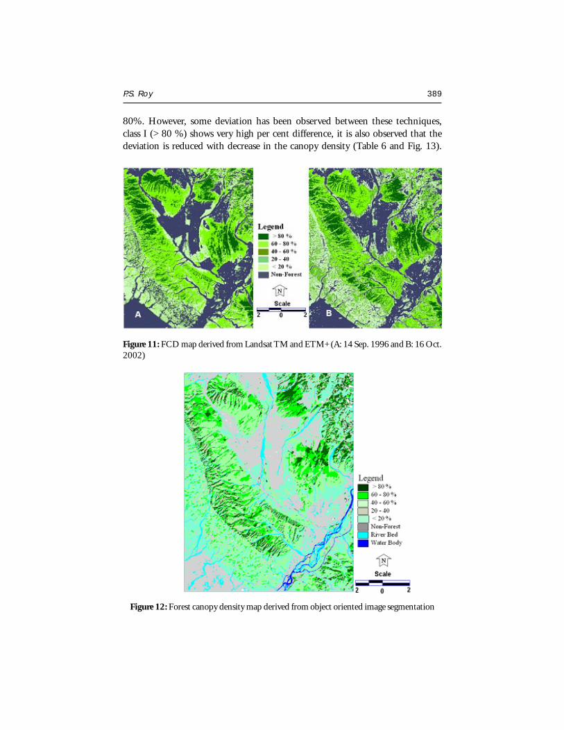
P.S. Roy 389
80%. However, some deviation has been observed between these techniques,class I (> 80 %) shows very high per cent difference, it is also observed that thedeviation is reduced with decrease in the canopy density (Table 6 and Fig. 13).
Figure 11: FCD map derived from Landsat TM and ETM+ (A: 14 Sep. 1996 and B: 16 Oct.2002)
Figure 12: Forest canopy density map derived from object oriented image segmentation
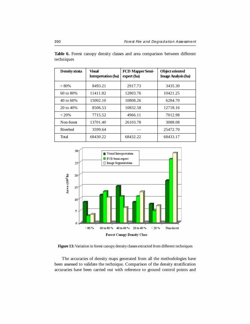
390 Forest Fire and Degradation Assessment
Table 6. Forest canopy density classes and area comparison between differenttechniques
Density strata Visual FCD Mapper Semi- Object orientedInterpretation (ha) expert (ha) Image Analysis (ha)
> 80% 8493.21 2917.73 3435.30
60 to 80% 11411.82 12803.76 10421.25
40 to 60% 15002.10 10808.26 6284.70
20 to 40% 8506.53 10832.58 12718.16
< 20% 7715.52 4966.11 7012.98
Non-forest 13701.40 26103.78 3088.08
Riverbed 3599.64 — 25472.70
Total 68430.22 68432.22 68433.17
Figure 13: Variation in forest canopy density classes extracted from different techniques
The accuracies of density maps generated from all the methodologies havebeen assessed to validate the technique. Comparison of the density stratificationaccuracies have been carried out with reference to ground control points and
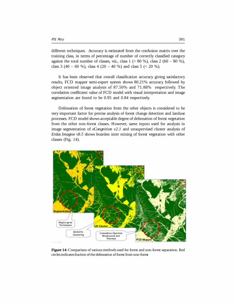
P.S. Roy 391
different techniques. Accuracy is estimated from the confusion matrix over thetraining class, in terms of percentage of number of correctly classified categoryagainst the total number of classes, viz., class 1 (> 80 %), class 2 (60 – 80 %),class 3 (40 – 60 %), class 4 (20 – 40 %) and class 5 (< 20 %).
It has been observed that overall classification accuracy giving satisfactoryresults, FCD mapper semi-expert system shows 80.21% accuracy followed byobject oriented image analysis of 87.50% and 71.88% respectively. Thecorrelation coefficient value of FCD model with visual interpretation and imagesegmentation are found to be 0.95 and 0.84 respectively.
Delineation of forest vegetation from the other objects is considered to bevery important factor for precise analysis of forest change detection and landuseprocesses. FCD model shows acceptable degree of delineation of forest vegetationfrom the other non-forest classes. However, same inputs used for analysis inimage segmentation of eCongnition v2.1 and unsupervised cluster analysis ofErdas Imagine v8.5 shows boarden inter mixing of forest vegetation with otherclasses (Fig. 14).
Figure 14: Comparison of various methods used for forest and non-forest separation. Redcircles indicates fraction of the delineation of forest from non-forest
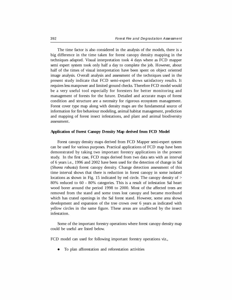
392 Forest Fire and Degradation Assessment
The time factor is also considered in the analysis of the models, there is abig difference in the time taken for forest canopy density mapping in thetechniques adapted. Visual interpretation took 4 days where as FCD mappersemi expert system took only half a day to complete the job. However, abouthalf of the times of visual interpretation have been spent on object orientedimage analysis. Overall analysis and assessment of the techniques used in thepresent study indicate that FCD semi-expert shows satisfactory results. Itrequires less manpower and limited ground checks. Therefore FCD model wouldbe a very useful tool especially for foresters for better monitoring andmanagement of forests for the future. Detailed and accurate maps of forestcondition and structure are a necessity for rigorous ecosystem management.Forest cover type map along with density maps are the fundamental source ofinformation for fire behaviour modeling, animal habitat management, predictionand mapping of forest insect infestations, and plant and animal biodiversityassessment.
Application of Forest Canopy Density Map derived from FCD Model
Forest canopy density maps derived from FCD Mapper semi-expert systemcan be used for various purposes. Practical applications of FCD map have beendemonstrated by taking two important forestry applications in the presentstudy. In the first case, FCD maps derived from two data sets with an intervalof 6 years i.e., 1996 and 2002 have been used for the detection of change in Sal(Shorea robusta) forest canopy density. Change detection assessment of thistime interval shows that there is reduction in forest canopy in some isolatedlocations as shown in Fig. 15 indicated by red circle. The canopy density of >80% reduced to 60 - 80% categories. This is a result of infestation Sal heartwood borer around the period 1998 to 2000. Most of the affected trees areremoved from the stand and some trees lost canopy and became moribundwhich has crated openings in the Sal forest stand. However, some area showsdevelopment and expansion of the tree crown over 6 years as indicated withyellow circles in the same figure. These areas are unaffected by the insectinfestation.
Some of the important forestry operations where forest canopy density mapcould be useful are listed below.
FCD model can used for following important forestry operations viz.,
To plan afforestation and reforestation activities
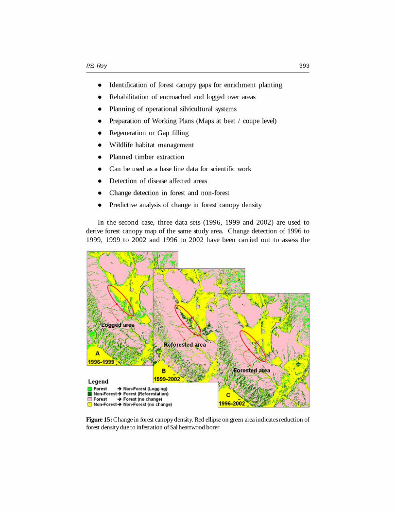
P.S. Roy 393
Identification of forest canopy gaps for enrichment planting
Rehabilitation of encroached and logged over areas
Planning of operational silvicultural systems
Preparation of Working Plans (Maps at beet / coupe level)
Regeneration or Gap filling
Wildlife habitat management
Planned timber extraction
Can be used as a base line data for scientific work
Detection of disease affected areas
Change detection in forest and non-forest
Predictive analysis of change in forest canopy density
In the second case, three data sets (1996, 1999 and 2002) are used toderive forest canopy map of the same study area. Change detection of 1996 to1999, 1999 to 2002 and 1996 to 2002 have been carried out to assess the
Figure 15: Change in forest canopy density. Red ellipse on green area indicates reduction offorest density due to infestation of Sal heartwood borer
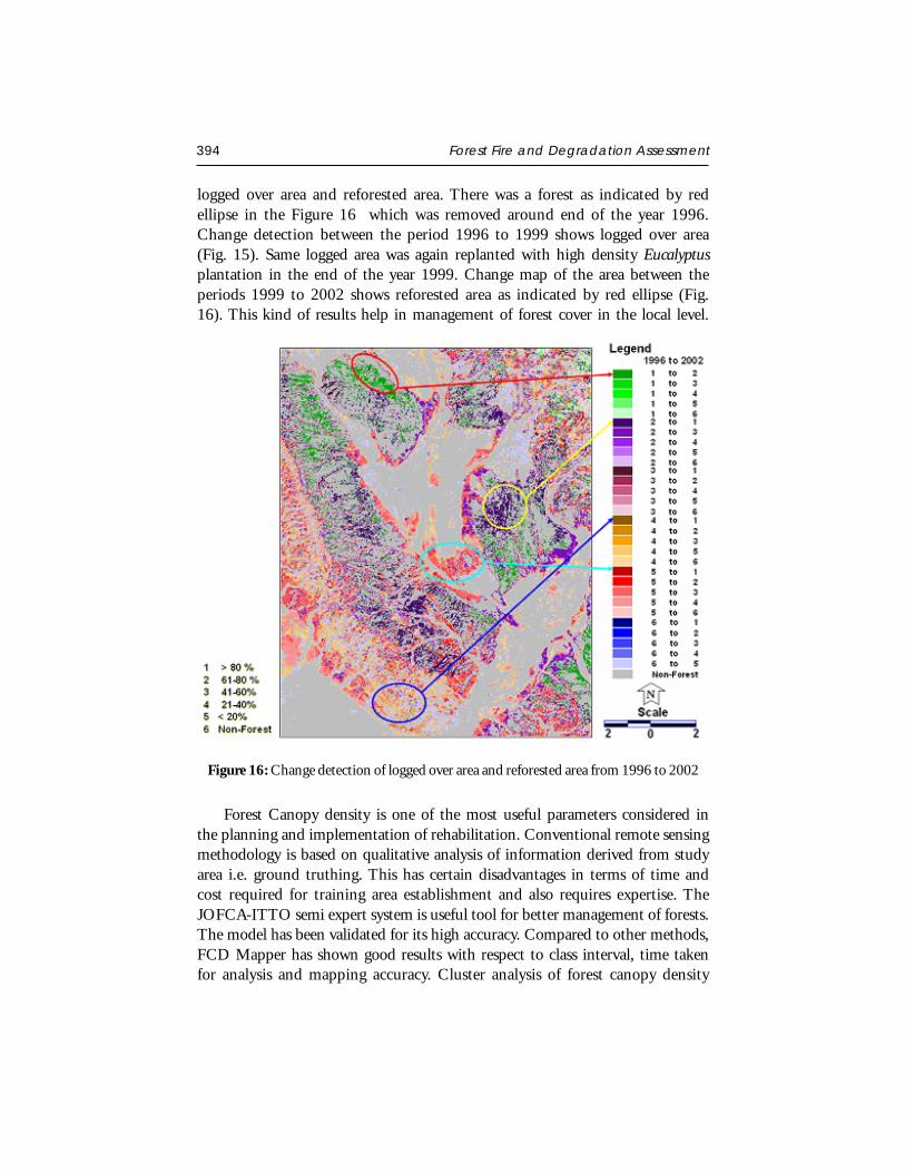
394 Forest Fire and Degradation Assessment
Figure 16: Change detection of logged over area and reforested area from 1996 to 2002
logged over area and reforested area. There was a forest as indicated by redellipse in the Figure 16 which was removed around end of the year 1996.Change detection between the period 1996 to 1999 shows logged over area(Fig. 15). Same logged area was again replanted with high density Eucalyptusplantation in the end of the year 1999. Change map of the area between theperiods 1999 to 2002 shows reforested area as indicated by red ellipse (Fig.16). This kind of results help in management of forest cover in the local level.
Forest Canopy density is one of the most useful parameters considered inthe planning and implementation of rehabilitation. Conventional remote sensingmethodology is based on qualitative analysis of information derived from studyarea i.e. ground truthing. This has certain disadvantages in terms of time andcost required for training area establishment and also requires expertise. TheJOFCA-ITTO semi expert system is useful tool for better management of forests.The model has been validated for its high accuracy. Compared to other methods,FCD Mapper has shown good results with respect to class interval, time takenfor analysis and mapping accuracy. Cluster analysis of forest canopy density
P.S. Roy 395
map derived from FCD Mapper and Conventional methods have showed similartrends with respect to percent area of forest and non-forest. Gregariousoccurrence of bushy vegetation like Lantana poses problem in delineation offorest canopy density as their reflectance is similar to that of the forest. Furtherimprovement can done to incorporate geographic coordinate system, mapcomposition and one click data import facility so that user can get the full-fledged utility of the semi expert system.
CONCLUSIONS
Increasing population pressure with multiplied demand for the domesticneeds have carved out separate fracture in the biosphere by modifying the forestecosystems. In the process we have been loosing green cover at faster rate thanexpected. Sustainable management of forest resources has become key agendaof the century. The assessment of the forest fire and degradation is one of theimportant factors to be considered for better management of the forest resources.However, the lack of reparative analysis with synoptic coverage has been one ofthe limitations in the conventional assessment techniques which can bepotentially over come by using geospatial approach. Hence, satellite remotesensing has provided holistic view to the planet Earth. The satellite remotesensing has enabled to map and monitor vegetation resources in varying scaleand time. The geographic information system enables to organize the data setsfor analysis and decision making process. India has made significant efforts tobuild state of art satellite systems and develop applications to manage the naturalresources. Forest cover mapping using space technology is already an operationaltool. Under a national scientific initiative India has developed comprehensivedata base on vegetation types, disturbance regimes, fragmentation and biologicalrichness at landscape level in the important eco-regions. Satellite images have aconsiderable value for mapping forest fire and degradation assessment. It helpsin decision making processes for the proper establishment of the green coverover the affected areas.
Extensive areas are burnt and deforested every year, leading to widespreadenvironmental and economic damage. The impact of this damage involves notonly the amount of timber burnt but also environmental damage to forestedlandscapes leading, in some cases, to land and forest degradation and theprevention of vegetation recovery. However, further more improvement requiredto enhance the process of better assessment, monitoring and management ofthe forest resources of the planet earth.
396 Forest Fire and Degradation Assessment
REFERENCES
Anonymous 1993. Rehabilitation of logged over Forests in Asia/Pacific region. Final Report ofSub Project II International Tropical Timber Organization- Japan Overseas ForestryConsultants Association, 1-78.
Abhineet Jainl, Shirish A. Ravan, R.K. Singh, K.K. Das and P.S. Roy, 1996. Forest fire riskmodelling using Remote Sensing and Geographic Information System . Current Science,70(10): 928-933.
Baret, F. J., G. P. W. Clevers, and M. D. Steven, 1995. The robustness of canopy gap fractionestimates from red and near-infrared reflectances: a comparison of approaches. RemoteSensing of Environment, 54(2): 141-151.
Bapedal. 1996. National Coordination Team on Land and Forest Fire Management. Int.Forest Fire News, No. 14, 27-28.
BAPPENAS. 1992. International Workshop on Long-Term Integrated Forest Fire Managementin Indonesia, Bandung, 17-18 June 1992. BAPPENAS/GTZ, Jakarta, Indonesia. 34 p.(mimeo).
Bartlett, H.H. 1955, 1957, 1961. Fire in relation to primitive agriculture and grazing in thetropics : annotated bibliography, Vol. 1-3. Mimeo. Publ. Univ. Michigan Bot. Gardens,Ann Arbor, USA.
Blodgett, C., Jakubauskas, M., Price, K., and Martinko, E. 2000. Remote Sensing-basedGeostatistical Modeling of Forest Canopy Structure. ASPRS 2000 Annual Conference,Washington, D.C., May 22-26.
Chandrashekhar, M.B., Sarnam Singh, N.K. Das and P.S. Roy. 2002. Wildlife-Human conflictanalysis in Kalatop Khajjiar Wildlife Sanctuary, Himachal Pradesh: Geospatial approach.National Seminar on Relevance of Biosphere reserve, National parks and Wildlife sanctuaries(Protected Habitats) in present context. May 25-26, 2002, held at Gurukula KangriUniversity, Hardwar (U.A.).
Cole, M.M. 1986. The savannas. Biogeography and Botany. Academic Press, London, UK.
DeFries, R. S., M. C. Hansen, and J. R. G. Townshend, 2000. Global continuous fields ofvegetation characteristics: a linear mixture model applied to multi-year 8km AVHRRdata. International Journal of Remote Sensing, 21(6/7): 1389-1414.
De Ronde, C., J.G. Goldammer, D.D. Wade, and R.V. Soares 1990. Prescribed fire in industrialpine plantations. In: J.G. Doldammer (editor), Fire in the tropical biota. Ecosystemprocesses and global challenges. Ecological Studies 84. Springer-Verlag, Berlin-Heidelberg.pp. 216-272.
P.S. Roy 397
Ehrlich D., E.F. Lambin and J. Malingreau 1997. Biomass Burning and Broad-scale LandCover Changes in Western Africa. Remote Sensing of the Environment, 61: 201-209.
Fernandez A., P. Illera and J.L. Casanova 1997. Automatic Mapping of Surfaces Affected byForest Fires in Spain Using AVHRR NDVI Composite Image Data. Remote Sensing ofthe Environment, 60: 153-162.
Flasse S.P. and Ceccato P.S. 1996. A contextual algorithm for AVHRR fire detection,International Journal of Remote Sensing, 17(2): 419-424.
Goldammer, J.G. 1988. Rural land use and fires in the tropics. Agroforestry Systems, 6 : 235-253.
Goldammer, J.G. (ed.) 1990. Fire in the tropical biota. Ecosystem processes and globalchallenges. Ecological Studies 84, Berlin-Heidelberg : Springer-Verlag.
Goldammer, J.G., and S.R. Penafiel 1990. Fire in the pine-grassland biomes of tropical andsubtropical Asia. In : J.G. Goldammer (editor) Fire in the tropical biota. Ecosystemprocesses and global challenges. Ecological Studies 84. Srpinger-Verlag, Berlin-Heidelberg,Germany. pp. 44-62.
Goldammer, J.G. 1991. Tropical wildland fires and global changes : Prehistoric evidence,present fire regimes, and future trends. In : J.S. Levine (editor), Global biomass burning.The MIT Press, Cambridge, Massachussetts, USA. pp. 83-91.
Goldammer, J.G. 1993. Feuer in Waldokosystemen der Tropen and Subtropen. Birkhauser-Verlag, Basel-Boston, Schweiz. 251 p.
Goldammer, J.G. 1994. Interdisciplinary research projects for developing a global fire science.A paper presented at the 12th Confer. Forest Meteorology, October 26-28, 1993, JekyllIsland, Georgia. Society of American Foresters Publ. 94-02 : 6-22.
Goldammer, J.G., B. Seibert, and W. Schindele. 1996. Fire in dipterocarp forests. In : A.Scheulte and D. Schone (editors), Dipterocarp forest ecosystems : Towards sustainablemanagement. World Scientific Publ., Singapore-New Jersey-London-Hongkong. pp.155-185.
Iverson, L. R., E. A. Cook, and R. L. Graham, 1989. A technique for extrapolating andvalidating forest cover across large regions: calibrating AVHRR data with TM data.International Journal of Remote Sensing 10(11): 1805-1812.
Justice C.O., and Dowty P. 1993. IGBP-DIS Satellite fire detection alogrithm workshoptechnical report. IGBP-DIS Working Paper No. 9, 88pp., Feb. 1993, NASA/GSFC,Greenbelt, Maryland, USA.
398 Forest Fire and Degradation Assessment
IFFM (Integrated Forest Fire Management Project). 1996. Integrated Forest Fire ManagementProject in East Kalimantan. Int. Forest Fire News, 14 : 29-30.
IFFN (International Forest Fire News), 2002. Fire Situation In India. Int. Forest Fire News,26: 23-27.
IGAC (International Global Atmospheric Chemistry Project). 1992. Biomass BurningExperiment : Impact on the Atmosphere and Biosphere. An Activity of the InternationalGlobal Atmospheric Chemistry (IGAC) Project, IGAC Core Project Office. The MITPress, Cambridge, Massachussetts, USA. 19 pp. + App.
Kasischke, E.S., L. L. Bourgeau-Chavez and N.H.F. French 1994. Observations of Variationsin ERS-1 SAR Image Intensity Associated with Forest Fires in Alaska. IEEE Transactionson Geoscience and Remote Sensing, 32(1): 206-210.
Komarek, E.V. 1968. Lightning and lightning fires as ecological forces. In : Proc. Ann. TallTimbers Fire Ecol. Conf. 8. Tall Timbers Research Station. Tallahassee, Florida, USA. pp.169-197.
Kowal, N.E. 1966. Shifting cultivation, fire and pine forest in the Cordillera Central, Luzon,Philippines. Ecol. Monogr., 36 : 389-419.
Luckman, A., J. Baker, T. M. Kuplich, C. C. Yanasse and A.C. Frery 1997. A Study of therelationship between Radar Backscatter and Regenerating Tropical Forest Biomass forSpaceborne SAR Instruments. Remote Sensing of the Environment, 60: 1-13.
Maselli, F. C., Conese, T. D. Filippis, and S. Norcini, 1995. Estimation of forest parametersthrough fuzzy classification of TM data. IEEE Transactions on Geoscience and RemoteSensing, 33 (1): 77-84.
Noble, B. 1990. Socio-economic and cultural background of forest fires in the Benguet pineforests. FAO TCP Assistance in Forest Fire Management, the Philippines Working PaperNo. 2. FAO Rome, TCP/PHI/8955, 50 p. (mimeo).
Nye, P. H., and D.J. Greenland. 1960. The soil under shifting cultivation. Tech. Comm. 51,Commonwelath Bureau of Soils. Harpenden, UK.
Otsuka, M. 1991. Forest management and farmers. Towards the sustainable land use – A casestudy from East Kalimantan, Indonesia. Master Program of Environmental Sciences.The University of Tsukuba, Japan (unpubl.).
Pancel, L., and C. Wiebecke 1981. “Controlled Burning” in subtropischen Kiefernwaldernund seine Auswirkungen auf Erosion and Artenminderung im Staate Uttar Pradesh.Forstarchiv, 52 : 61-63.
P.S. Roy 399
Phillips, J. 1965. Fire as master and servant : its influence in the bioclimatic regions of Trans-Saharat Africa. In : Proc. Tall Timbers Fire Ecol. Conf. 4. Tall Timbers Research Station.Tallahassee, Florida, USA. pp. 7-109.
Porwal, M.C., M.J.C. Meir, Y.A. Hussin and P.S. Roy : 1997 : Spatial Modelling for fire riskzonation using Remote Sensing and GIS. Paper presented in ISPRS Commission VIIWorking Group II Workshop on Application of Remote Sensing and GIS for SustainableDevelopment, Hyderabad, 1997.
Prins, E.M., and Menzel, W.P. 1992. Geostationary satellite detection of biomass burning inSouth America. International Journal of Remote Sensing, 13(15): 2783-3462.
Rikimaru, A. 1996. LANDSAT TM Data Processing Guide for forest Canopy Density Mappingand Monitoring Model. ITTO workshop on utilization of remote sensing in site assessmentand planning for rehabilitation of logged-over forest. Bangkok, Thailand, July 30- August1,1996.1-8.
Roy, P.S., R.N. Kaul, M.R. Sharma Roy and S.G. Garbyal, 1985. Forest type stratification anddelineation of shifting cultivation areas in eastern part of Arunachal Pradesh using LandsatMSS data. International Journal of Remote Sensing, 6(3): 411-418.
Roy, P.S., Diwakar, P.G., Vohra, T.P.S. and Bhan, S.K.1990. Forest Resource Managementusing Indian Remote Sensing Satellite data. Asian -Pacific Remote Sensing J. 3 (1): 11-22.
Roy, P.S., S. Miyatake and A. Rikimaru, 1997. Biophysical Spectral Response Modeling Approachfor Forest Density Stratification. Proc.The 18th Asian Conference on Remote Sensing,October 20-24, 1997, Malaysia.
Steyaert, L.T., F.G. Hall and T.R. Loveland 1997. Land Cover Mapping, Fire Regeneration,and Scaling Studies in the Canadian Boreal Forest with 1-km AVHRR and Landsat TMdata. Journal of Geophysical Research, 102(d24): 29581-29598.
Stott, P., J.G. Goldammer, and W.L. Werner. 1990. The role of fire in the tropical lowlanddeciduous forests of Asia. In : J.G. Goldammer (editor), Fire in the tropical biota.Ecosystem processes and global challenges. Ecological Studies 84. Springer-Verlag. Berlin-Heidelberg, Germany, pp. 21-44.
Stuttard, M., S. Boardman, P. Ceccato, I. Downey, S. Flasse, M. Gooding and K. Muirhead,1995. Global Vegetation Fire Product. Final Report to the JRC. Contract 100444-94-09-FIEP ISP GB. Earth Observation Sciences Ltd.
Viedma, O., J. Meli, D. Segarra and J. Garc’a-Haro 1997. Modeling Rates of EcosystemRecovery after Fires by Using Landsat TM data. Remote Sensing of Environment, 61:383-398.

400 Forest Fire and Degradation Assessment
Watters, R.F. 1971. Shifting cultivation in Latin America. FAO for Dev. Pap. 17. Food andAgricultural Organisation of the United Nations, Rome, Italy.
Zhu, Z. and D. L. Evans, 1994. US forest types and predicted percent forest cover fromAVHRR data. Photogrammetric Engineering & Remote Sensing, 60(5): 525-531.
DESERT LOCUST MONITORING SYSTEM –REMOTE SENSING AND GIS BASED APPROACH
D. Dutta, S. Bhatawdekar, B. Chandrasekharan, J.R. Sharma,S. Adiga*, Duncan Wood** and Adrian McCardle**Regional Remote Sensing Service Centre, CAZRI Campus, Jodhpur, Rajasthan* NNRMS/RRSSC, ISRO Headquarters, Bangalore** RADARSAT International, Richmond BC, Vancouver, Canada
Abstract : Desert locusts (DL) are a serious problem during April to August in thedeserts and semi-deserts of Republic of Kazakhstan and causing extensive cropdamage. There is no institutional and functional mechanism to forecast the habitatof locusts and most of the area remains unnoticed after laying eggs. The key toimprove DL forecasting and control depends on the collection and generation ofhistorical database on locust, weather and habitat from affected region. Looking atthe problem a Decision Support System (DSS) has been developed on ARC/INFOGIS with ergonomic user interface for ingestion and subsequent analysis of locustrelated information vis-à-vis bio-physical and climatic data acquired from varioussatellite sensors and hydromet weather server respectively to identify high frequencybreeding areas well before the physiological development is completed. Weatherbased analytical models for physiological development of DL has been dovetailedwith the DSS for facilitating historic and present data analysis in relation to locustactivity. This will enhance the surveying capability and better forecasting.
INTRODUCTION
Desert locusts (Schistocerca gregaria, Forskl) are known to be one of thedreaded insects since time immemorial for agricultural production. More than60 countries are affected at varying degrees during plague development causedby several consecutive generation of successful breeding triggered by afavourable sequence of heavy and widespread rainfall. Normally in solitaryphase density remains low and poses no economic threat but under favourablebio-climatic condition population increases very fast over space and time andforms gregarious swarms which can devastate agricultural lands. It is duringthis period that locusts can cause enormous damage to standing crops even
Satellite Remote Sensing and GIS Applications in Agricultural Meteorologypp. 401-423
402 Desert Locust Monitoring System - Remote Sensing ...
several hundred kilometers away from their origin. However, early detectionof locust growth and breeding sites are two key issues for efficient surveillanceand control of desert locusts (DL). Locating high frequency breeding areasover temporal and spatial scale warrants analysis of large number of biophysicaland bio-climatic variables in relation to locust physiology. Nevertheless themost difficult part of forecasting is migration of adult winged locusts, whichis influenced by large number of weather parameters at synoptic scale.
To manage the locust devastation and its timely warning there is a needfor structured geospatial database in GIS environment and interfacing withother analytical and modeling tools to form sophisticated spatial DecisionSupport System (Healy et al., 1996). This paper describes one such systemand the approach to meet forecasting need using ARC/INFO GIS and a hostof digital data especially from optical and microwave satellites sensors. GISand Remote Sensing technology dramatically improves the ability of forecastingthrough effective manipulation of large volume and variety of spatiallyreferenced and descriptive data. The logical aspects of database design employsintegration of all application requirements in a database structure that supportsthe view and processing needs of these applications. The physical aspects refersto evalusation of alternative implementations and choosing storage structure,query mechanism and access methods (Navathe and Schkolnik, 1978).
The major plague of 1985-89 prompted the world acridologists to improvethe forecasting tools and methodologies in order to maximize the effectivenessof pesticides and reduce the toxicity in aquatic environment. The highestpriority was assigned to modeling and validating the spread of infestationsover space and time in relation to concurrent changes in weather and vegetation(FAO, 1989).
In the present study effort has been made to provide interface to handlepopulation dynamics, physiological development, habitat suitability as wellas climate suitability for breeding and migration. The locusts biology inrelation to weather and other environmental factors have been used inforecasting process. The DSS essentially adheres with norms of database designstandard, customization, validation, integration before actual query mechanismand performing modeling operations.
Locusts in Kazakhstan
Locusts are a recurring problem in Kazakhstan but the problem has beenintensified since 1996 mostly due to collapse of uncompetitive farming and

D. Dutta, et al. 403
unusually warm weather in recent past. In 2000, 27% of total food grainproduction i.e. 5 million ton was destroyed and more than 8.8 million haland was affected. The perennial dynamics of locust population has strongrelationship with transformation of landuse fabric in the republic from 1954to 1992 onwards. The landuse distribution of Kazakhstan is dominated bysemi desert and deserts (77.2%), and grassland and forests of 9.4%. Thegrasslands used to serve as ecological niche for the desert locusts confined tosmaller pockets from which they used to migrate in adjoining fringe ofagricultural lands. But the land development history of Kazakhstan hasadversely affected the natural habitats of locusts while passing through 4different phases since 1954.
i. Active development of virgin and fallow lands (1954-1964).
ii. Use of soil protection system in agriculture (1965-1974).
iii. Intensive use of agrotechnology (1976-1992) and indiscriminate useof pesticides which has caused locust insurgence.
iv. Continuous shrinking of agricultural lands due to economicconstraints, giving rise to multistage fallow (1992 onwards).
As a result of this multi-phasic land transformation large portion of arablelands have been infested with wild grasses and bushes. The extent of suchlands has largely expanded and redistributed in the contact zones betweencultivated and uncultivated lands in the territory forming excellent habitatfor DL scattered over large areas especially in the west, south-east and south.Out of 35 species of DL found in Kazakhstan mostly 3 types are dominatingnamely Asian, Italian and Moroccan. In the east Italian locusts (Calliptamusitalicus) dominate, whereas in south-east Asian locusts (Locusta migratoria) andin south Moroccan locusts (Dociostaurus maroccanus) are prevalent. Thesituation is getting worse not only in Kazakhstan but also in adjoining countriesviz. Russia, Uzbekistan and Kyrgystan. The locusts are also spreading fromtheir traditional breeding grounds to further west. Many new areas have beenreported first time since 80 years.
Key issues in DL control
The major issues related to DL control can be summarized as follows.
404 Desert Locust Monitoring System - Remote Sensing ...
Acquisition of bio-physical information from vast inaccessible and hostileterrain (locust habitats) using satellite remote sensing technology withbetter temporal sampling capability.
Parameterization and accurate translation of remote sensing informationin relation to ground segment for model input.
Use of spatial variables for process modeling and subsequent field validation.
Bio-climatic modeling for locust physiology and migration based uponhistorical locust events and ground intelligence.
Operationalization for forecasting of high frequency breeding areas andflight behavior.
Satellite remote sensing helps to examine relationships betweendistributions of insect pests, rainfall and green vegetation in the seasonallydry tropics. For migration and dispersal modeling there is a need for studyinghistorical records for plague development and forecasting. Current weather datacould help to examine downwind airborne dispersal of insect pests over a rangeof temporal and spatial scales. Based upon the survey of ecological conditionsin potential breeding and outbreak areas, aerial and ground survey is organizedthat become potentially suitable after rainfall incidence. Following the surveyoperation strategies are chalked out to control DL populations when exceedsabove a specific threshold limit, mainly in known outbreak areas.
Requirement for a GIS to support Forecasting
DSS facilitates incorporation and integration of a variety of information,relevant for modeling of locust population on spatial and temporal contexton a common platform. It maximizes the opportunities for early interventionand management of locust swarms. Characteristically it is ergonomic with userinterface to facilitate both data capture and analysis through a series of menusfor accessing separate information management tools with data display onspatial context. It is desirable to bring together all the information sourcesused by forecasting and field staff to aid in decision making process. Thecharacteristic features of the DSS are expected to be as follows (Healey et al.,1996).
i. Access to historical records of locust sightings and associated environmentalconditions, with ability to cross-reference related events.
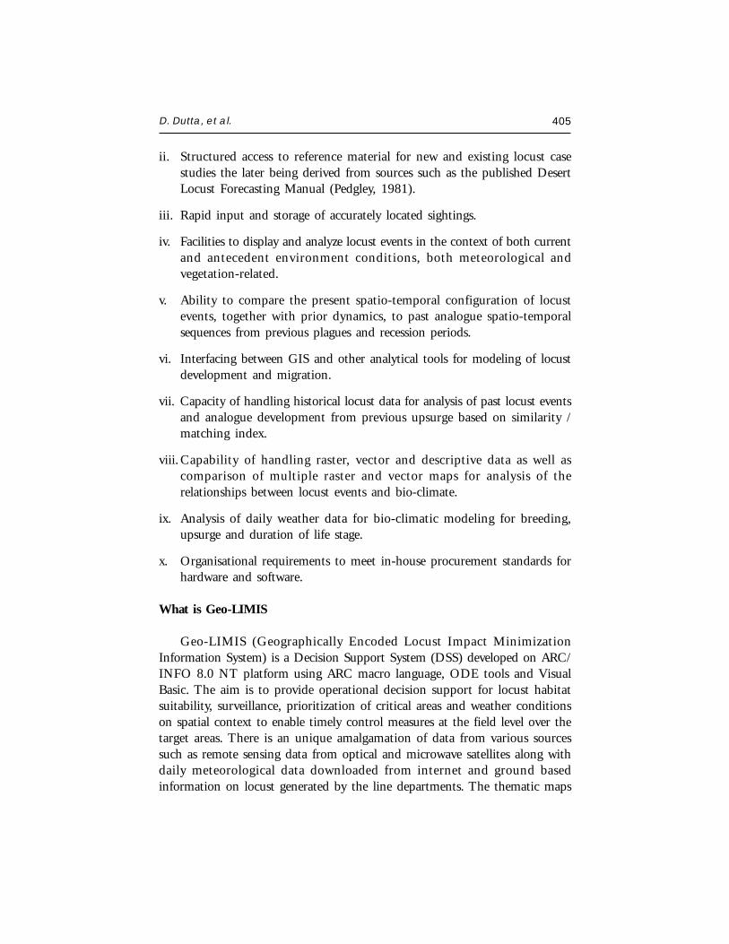
D. Dutta, et al. 405
ii. Structured access to reference material for new and existing locust casestudies the later being derived from sources such as the published DesertLocust Forecasting Manual (Pedgley, 1981).
iii. Rapid input and storage of accurately located sightings.
iv. Facilities to display and analyze locust events in the context of both currentand antecedent environment conditions, both meteorological andvegetation-related.
v. Ability to compare the present spatio-temporal configuration of locustevents, together with prior dynamics, to past analogue spatio-temporalsequences from previous plagues and recession periods.
vi. Interfacing between GIS and other analytical tools for modeling of locustdevelopment and migration.
vii. Capacity of handling historical locust data for analysis of past locust eventsand analogue development from previous upsurge based on similarity /matching index.
viii. Capability of handling raster, vector and descriptive data as well ascomparison of multiple raster and vector maps for analysis of therelationships between locust events and bio-climate.
ix. Analysis of daily weather data for bio-climatic modeling for breeding,upsurge and duration of life stage.
x. Organisational requirements to meet in-house procurement standards forhardware and software.
What is Geo-LIMIS
Geo-LIMIS (Geographically Encoded Locust Impact MinimizationInformation System) is a Decision Support System (DSS) developed on ARC/INFO 8.0 NT platform using ARC macro language, ODE tools and VisualBasic. The aim is to provide operational decision support for locust habitatsuitability, surveillance, prioritization of critical areas and weather conditionson spatial context to enable timely control measures at the field level over thetarget areas. There is an unique amalgamation of data from various sourcessuch as remote sensing data from optical and microwave satellites along withdaily meteorological data downloaded from internet and ground basedinformation on locust generated by the line departments. The thematic maps
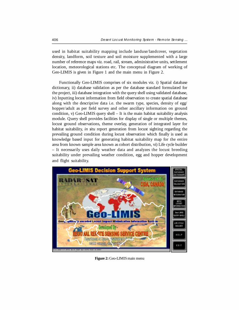
406 Desert Locust Monitoring System - Remote Sensing ...
used in habitat suitability mapping include landuse/landcover, vegetationdensity, landform, soil texture and soil moisture supplemented with a largenumber of reference maps viz. road, rail, stream, administrative units, settlementlocation, meteorological stations etc. The conceptual diagram of working ofGeo-LIMIS is given in Figure 1 and the main menu in Figure 2.
Functionally Geo-LIMIS comprises of six modules viz. i) Spatial databasedictionary, ii) database validation as per the database standard formulated forthe project, iii) database integration with the query shell using validated database,iv) Inputting locust information from field observation to create spatial databasealong with the descriptive data i.e. the swarm type, species, density of egg/hopper/adult as per field survey and other ancillary information on groundcondition, v) Geo-LIMIS query shell – It is the main habitat suitability analysismodule. Query shell provides facilities for display of single or multiple themes,locust ground observations, theme overlay, generation of integrated layer forhabitat suitability, in situ report generation from locust sighting regarding theprevailing ground condition during locust observation which finally is used asknowledge based input for generating habitat suitability map for the entirearea from known sample area known as cohort distribution, vi) Life cycle builder– It necessarily uses daily weather data and analyzes the locust breedingsuitability under prevailing weather condition, egg and hopper developmentand flight suitability.
Figure 2: Geo-LIMIS main menu
D. Dutta, et al. 407
Spatial Database Dictionary
The package has devised suitable database structure for spatial and non-spatial database elements. Database elements, required to be integrated, withthe package must adhere to these standards. To explore and analyze thesedatabase elements efficiently and provide ease to the users in executing varioustasks of the package, all the database elements and components should beknown to the shell. For this purpose, Geo-LIMIS maintains a spatial databasedictionary, named as LWTHEME.LWS (INFO table), to store details of variousdatabase elements. This dictionary can be updated and extended by the userthrough a user friendly GUI (Figure 3). User can browse through the spatialdictionary, update or extend it.
Message board
Figure 3: Spatial database dictionary interface
This module (Figure 4) performs the validation of each database element(spatial layers) and also checks the integrity of the database and validates eachdatabase element whether it adheres to Geo-LIMIS database design andstandards or not. It generates a validation report after critically examining thedata. The spatial database elements, which have an entry in the spatial databasedictionary will only be considered for validation. During database validationthe package performs following validation checks vis-à-vis Geo-LIMIS databasedesign and standards.
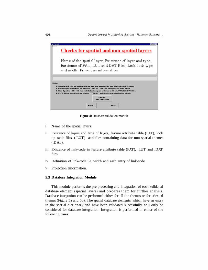
408 Desert Locust Monitoring System - Remote Sensing ...
i. Name of the spatial layers.
ii. Existence of layers and type of layers, feature attribute table (FAT), lookup table files. (.LUT) and files containing data for non-spatial themes(.DAT).
iii. Existence of link-code in feature attribute table (FAT), .LUT and .DATfiles.
iv. Definition of link-code i.e. width and each entry of link-code.
v. Projection information.
5.3 Database Integration Module
This module performs the pre-processing and integration of each validateddatabase element (spatial layers) and prepares them for further analysis.Database integration can be performed either for all the themes or for selectedthemes (Figure 5a and 5b). The spatial database elements, which have an entryin the spatial dictionary and have been validated successfully, will only beconsidered for database integration. Integration is performed in either of thefollowing cases.
Figure 4: Database validation module
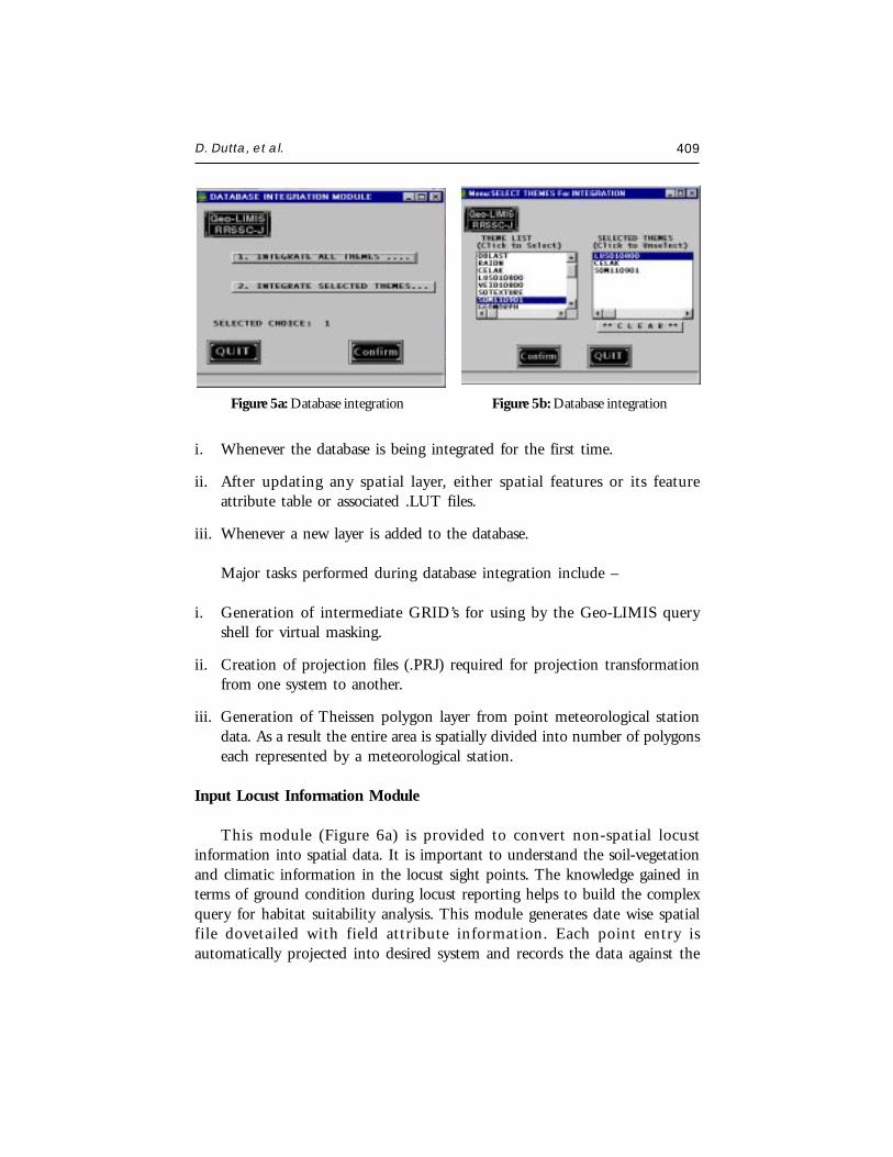
D. Dutta, et al. 409
i. Whenever the database is being integrated for the first time.
ii. After updating any spatial layer, either spatial features or its featureattribute table or associated .LUT files.
iii. Whenever a new layer is added to the database.
Major tasks performed during database integration include –
i. Generation of intermediate GRID’s for using by the Geo-LIMIS queryshell for virtual masking.
ii. Creation of projection files (.PRJ) required for projection transformationfrom one system to another.
iii. Generation of Theissen polygon layer from point meteorological stationdata. As a result the entire area is spatially divided into number of polygonseach represented by a meteorological station.
Input Locust Information Module
This module (Figure 6a) is provided to convert non-spatial locustinformation into spatial data. It is important to understand the soil-vegetationand climatic information in the locust sight points. The knowledge gained interms of ground condition during locust reporting helps to build the complexquery for habitat suitability analysis. This module generates date wise spatialfile dovetailed with field attribute information. Each point entry isautomatically projected into desired system and records the data against the
Figure 5a: Database integration Figure 5b: Database integration
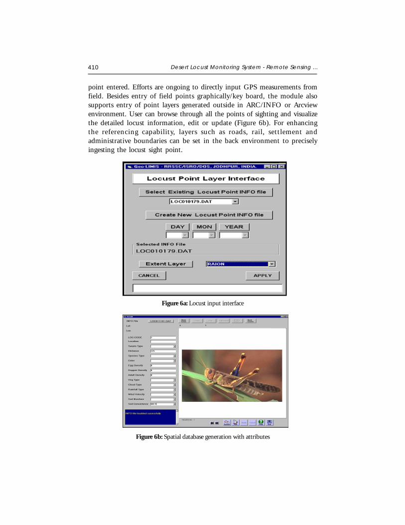
410 Desert Locust Monitoring System - Remote Sensing ...
point entered. Efforts are ongoing to directly input GPS measurements fromfield. Besides entry of field points graphically/key board, the module alsosupports entry of point layers generated outside in ARC/INFO or Arcviewenvironment. User can browse through all the points of sighting and visualizethe detailed locust information, edit or update (Figure 6b). For enhancingthe referencing capability, layers such as roads, rail, settlement andadministrative boundaries can be set in the back environment to preciselyingesting the locust sight point.
Figure 6a: Locust input interface
Figure 6b: Spatial database generation with attributes
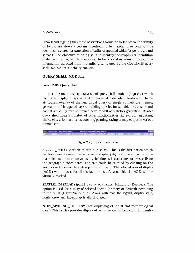
D. Dutta, et al. 411
From locust sighting files those observations would be sorted where the densityof locust are above a certain threshold to be critical. The points, thusidentified, are used for generation of buffer of specified width (as per the groundspread). The objective of doing so is to identify the biophysical conditionunderneath buffer, which is supposed to be critical in terms of locust. Theinformation extracted from the buffer area, is used by the Geo-LIMIS queryshell, for habitat suitability analysis.
QUERY SHELL MODULE
Geo-LIMIS Query Shell
It is the main display analysis and query shell module (Figure 7) whichfacilitates display of spatial and non-spatial data, identification of themeattributes, overlay of themes, visual query of single of multiple themes,generation of integrated layers, building queries for suitable locust sites andhabitat suitability map in desired scale as well as statistics generation. Besidesquery shell hosts a number of other functionalities viz. symbol updating,choice of text font and color, zooming/panning, saving of map output in variousformats etc.
Figure 7: Query shell main menu
SELECT_AOD (Selection of area of display): This is the first option whichfacilitates user to select desired area of display (Figure 8). Selection could bemade for one or more polygons, by defining as irregular area or by specifyingthe geographic coordinates. The area could be selected by clicking on thegraphics or by name through a pull down menu. The selected area of display(AOD) will be used for all display purpose. Area outside the AOD will bevirtually masked.
SPATIAL_DISPLAY (Spatial display of themes, Primary or Derived): Theoption is used for display of selected theme (primary or derived) pertainingto the AOD (Figure 9a, b, c, d). Along with map the legend, display scale,north arrow and index map is also displayed.
NON_SPATIAL _DISPLAY (For displaying of locust and meteorologicaldata): This facility provides display of locust related information viz. density
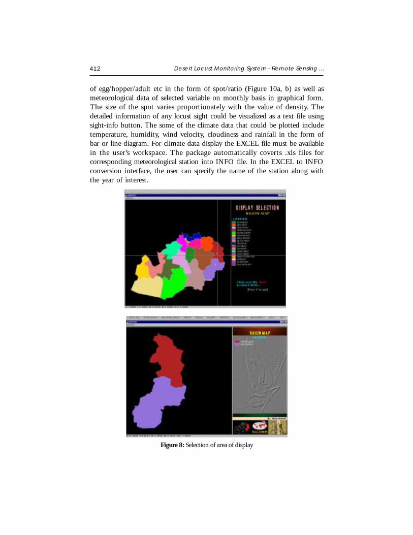
412 Desert Locust Monitoring System - Remote Sensing ...
of egg/hopper/adult etc in the form of spot/ratio (Figure 10a, b) as well asmeteorological data of selected variable on monthly basis in graphical form.The size of the spot varies proportionately with the value of density. Thedetailed information of any locust sight could be visualized as a text file usingsight-info button. The some of the climate data that could be plotted includetemperature, humidity, wind velocity, cloudiness and rainfall in the form ofbar or line diagram. For climate data display the EXCEL file must be availablein the user’s workspace. The package automatically coverts .xls files forcorresponding meteorological station into INFO file. In the EXCEL to INFOconversion interface, the user can specify the name of the station along withthe year of interest.
Figure 8: Selection of area of display

D. Dutta, et al. 413
IDENTIFY (To identify attribute of the themes at user specified location): Ithelps the user to identify attributes at user specified location (Figure 11).Identification could be for currently displayed theme, selected themes or multi-themes.
OVERLAY (For overlaying selected features of a theme on the displayedtheme): It facilitates the user to overlay selected features of a theme on thedisplayed theme. Overlaid theme is displayed in the form of polygon, lines,points or hatched polygons (for themes of GRID type) with selected color/pattern (Figure 12).
VIS_QUERY (For visual query of single or multiple themes): The purpose ofthis option is to perform visual query of single theme or across multiple themesi.e. to display selected subset of features (attributes) using query builder. Thearea satisfying the user defined query is only displayed (Figure 13). In thequery builder menu the name of the selected theme appears along with
Figure 9: Spatial display of themes
(A) (B)
(C) (D)
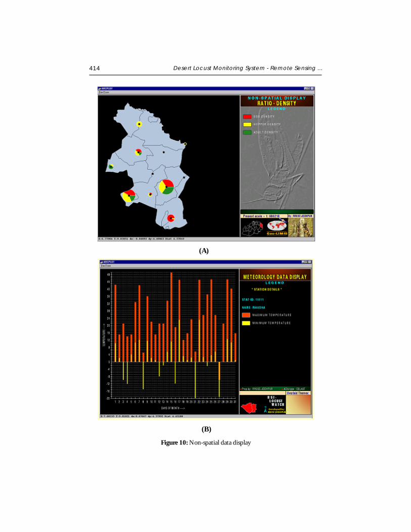
414 Desert Locust Monitoring System - Remote Sensing ...
Figure 10: Non-spatial data display
(A)
(B)
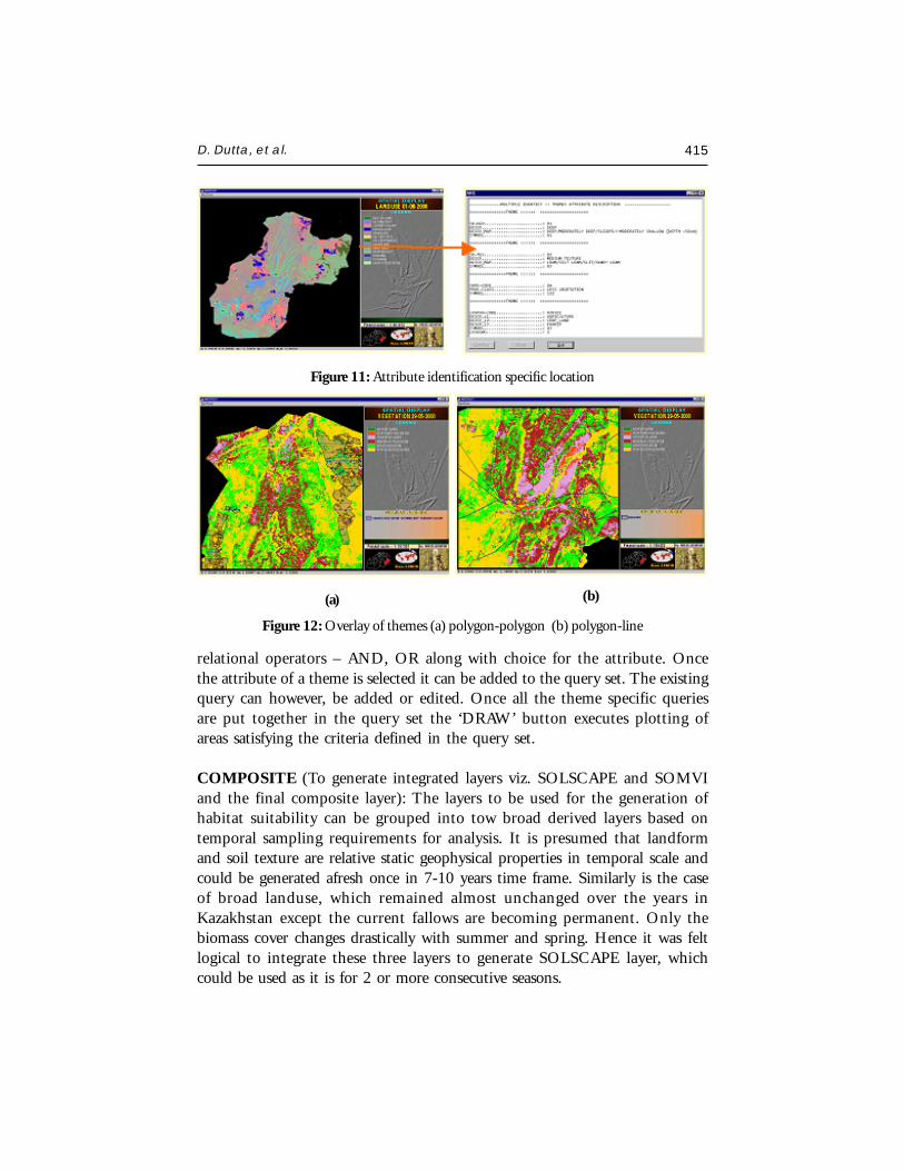
D. Dutta, et al. 415
relational operators – AND, OR along with choice for the attribute. Oncethe attribute of a theme is selected it can be added to the query set. The existingquery can however, be added or edited. Once all the theme specific queriesare put together in the query set the ‘DRAW’ button executes plotting ofareas satisfying the criteria defined in the query set.
COMPOSITE (To generate integrated layers viz. SOLSCAPE and SOMVIand the final composite layer): The layers to be used for the generation ofhabitat suitability can be grouped into tow broad derived layers based ontemporal sampling requirements for analysis. It is presumed that landformand soil texture are relative static geophysical properties in temporal scale andcould be generated afresh once in 7-10 years time frame. Similarly is the caseof broad landuse, which remained almost unchanged over the years inKazakhstan except the current fallows are becoming permanent. Only thebiomass cover changes drastically with summer and spring. Hence it was feltlogical to integrate these three layers to generate SOLSCAPE layer, whichcould be used as it is for 2 or more consecutive seasons.
Figure 11: Attribute identification specific location
Figure 12: Overlay of themes (a) polygon-polygon (b) polygon-line
(a) (b)
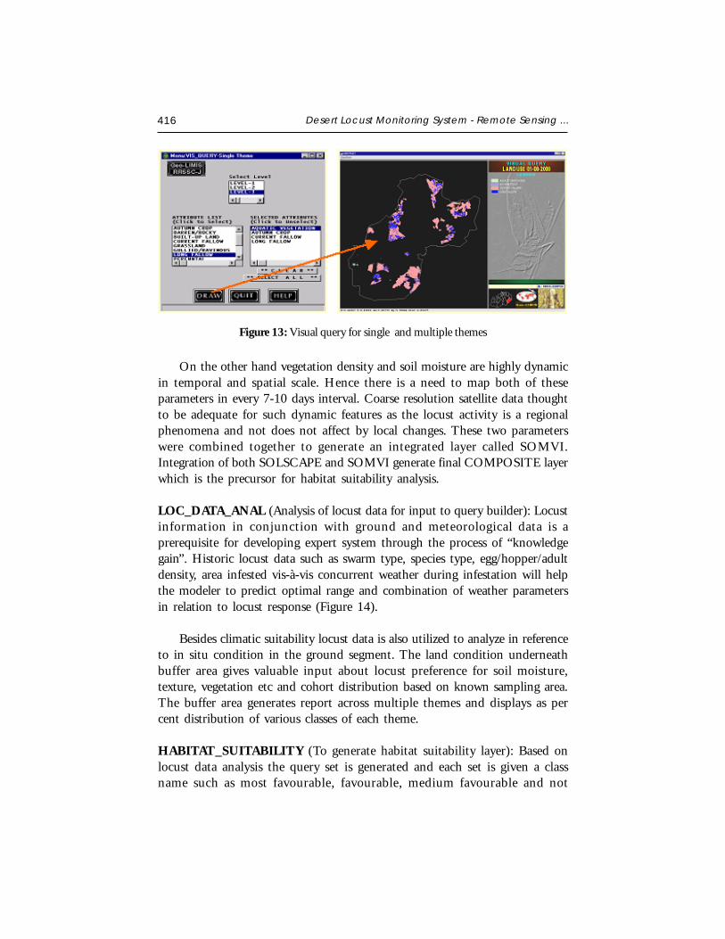
416 Desert Locust Monitoring System - Remote Sensing ...
On the other hand vegetation density and soil moisture are highly dynamicin temporal and spatial scale. Hence there is a need to map both of theseparameters in every 7-10 days interval. Coarse resolution satellite data thoughtto be adequate for such dynamic features as the locust activity is a regionalphenomena and not does not affect by local changes. These two parameterswere combined together to generate an integrated layer called SOMVI.Integration of both SOLSCAPE and SOMVI generate final COMPOSITE layerwhich is the precursor for habitat suitability analysis.
LOC_DATA_ANAL (Analysis of locust data for input to query builder): Locustinformation in conjunction with ground and meteorological data is aprerequisite for developing expert system through the process of “knowledgegain”. Historic locust data such as swarm type, species type, egg/hopper/adultdensity, area infested vis-à-vis concurrent weather during infestation will helpthe modeler to predict optimal range and combination of weather parametersin relation to locust response (Figure 14).
Besides climatic suitability locust data is also utilized to analyze in referenceto in situ condition in the ground segment. The land condition underneathbuffer area gives valuable input about locust preference for soil moisture,texture, vegetation etc and cohort distribution based on known sampling area.The buffer area generates report across multiple themes and displays as percent distribution of various classes of each theme.
HABITAT_SUITABILITY (To generate habitat suitability layer): Based onlocust data analysis the query set is generated and each set is given a classname such as most favourable, favourable, medium favourable and not
Figure 13: Visual query for single and multiple themes
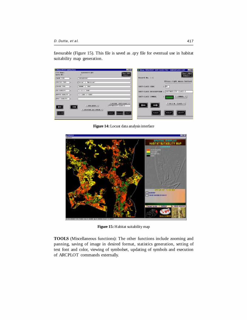
D. Dutta, et al. 417
favourable (Figure 15). This file is saved as .qry file for eventual use in habitatsuitability map generation.
Figure 14: Locust data analysis interface
Figure 15: Habitat suitability map
TOOLS (Miscellaneous functions): The other functions include zooming andpanning, saving of image in desired format, statistics generation, setting oftext font and color, viewing of symbolset, updating of symbols and executionof ARCPLOT commands externally.
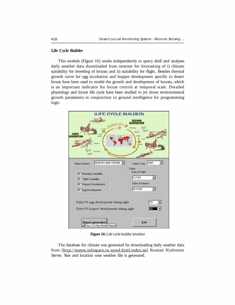
418 Desert Locust Monitoring System - Remote Sensing ...
Life Cycle Builder
This module (Figure 16) works independently to query shell and analysesdaily weather data downloaded from internet for forecasting of i) climatesuitability for breeding of locusts and ii) suitability for flight. Besides thermalgrowth curve for egg incubation and hopper development specific to desertlocust have been used to model the growth and development of locusts, whichis an important indicator for locust control at temporal scale. Detailedphysiology and locust life cycle have been studied to jot down environmentalgrowth parameters in conjunction to ground intelligence for programminglogic.
Figure 16: Life cycle builder interface
The database for climate was generated by downloading daily weather datafrom (http://meteo.infospace.ru.wond.html.index.ssi) Russian HydrometServer. Year and location wise weather file is generated.
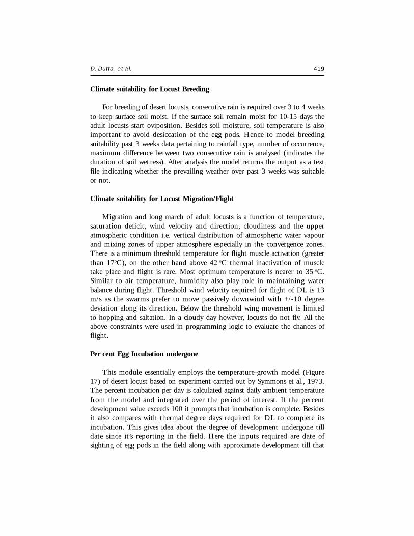
D. Dutta, et al. 419
Climate suitability for Locust Breeding
For breeding of desert locusts, consecutive rain is required over 3 to 4 weeksto keep surface soil moist. If the surface soil remain moist for 10-15 days theadult locusts start oviposition. Besides soil moisture, soil temperature is alsoimportant to avoid desiccation of the egg pods. Hence to model breedingsuitability past 3 weeks data pertaining to rainfall type, number of occurrence,maximum difference between two consecutive rain is analysed (indicates theduration of soil wetness). After analysis the model returns the output as a textfile indicating whether the prevailing weather over past 3 weeks was suitableor not.
Climate suitability for Locust Migration/Flight
Migration and long march of adult locusts is a function of temperature,saturation deficit, wind velocity and direction, cloudiness and the upperatmospheric condition i.e. vertical distribution of atmospheric water vapourand mixing zones of upper atmosphere especially in the convergence zones.There is a minimum threshold temperature for flight muscle activation (greaterthan 17oC), on the other hand above 42 oC thermal inactivation of muscletake place and flight is rare. Most optimum temperature is nearer to 35 oC.Similar to air temperature, humidity also play role in maintaining waterbalance during flight. Threshold wind velocity required for flight of DL is 13m/s as the swarms prefer to move passively downwind with +/-10 degreedeviation along its direction. Below the threshold wing movement is limitedto hopping and saltation. In a cloudy day however, locusts do not fly. All theabove constraints were used in programming logic to evaluate the chances offlight.
Per cent Egg Incubation undergone
This module essentially employs the temperature-growth model (Figure17) of desert locust based on experiment carried out by Symmons et al., 1973.The percent incubation per day is calculated against daily ambient temperaturefrom the model and integrated over the period of interest. If the percentdevelopment value exceeds 100 it prompts that incubation is complete. Besidesit also compares with thermal degree days required for DL to complete itsincubation. This gives idea about the degree of development undergone tilldate since it’s reporting in the field. Here the inputs required are date ofsighting of egg pods in the field along with approximate development till that
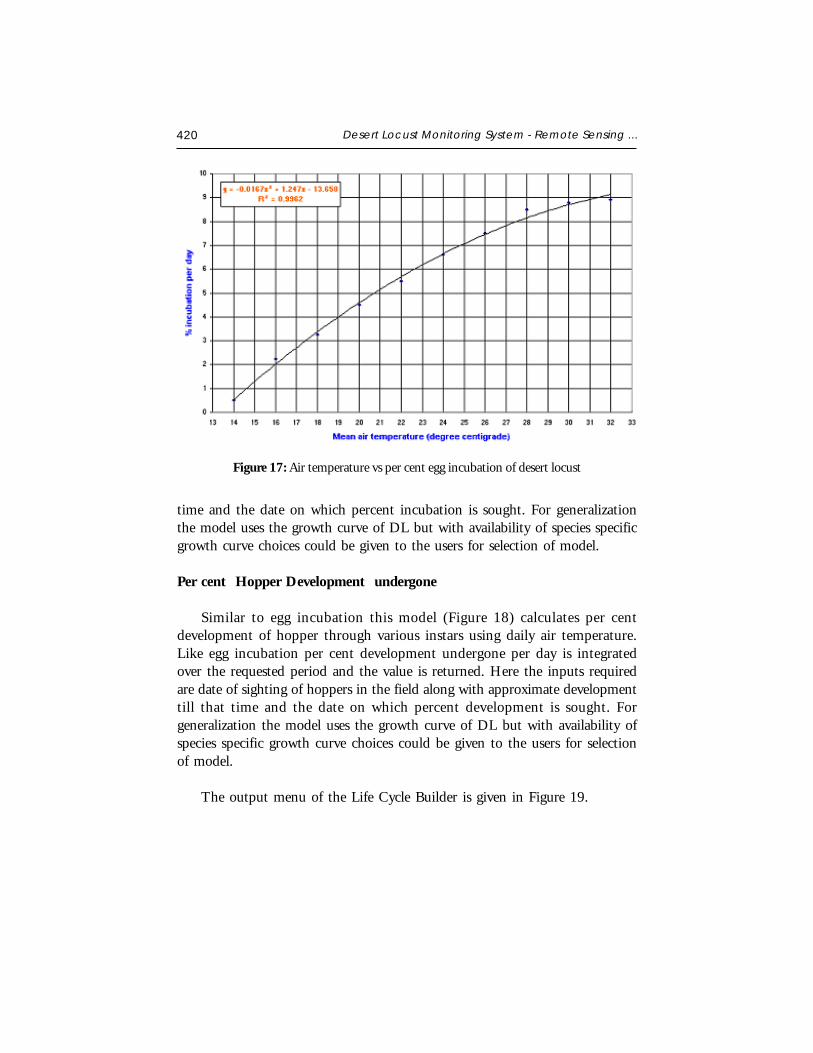
420 Desert Locust Monitoring System - Remote Sensing ...
Figure 17: Air temperature vs per cent egg incubation of desert locust
time and the date on which percent incubation is sought. For generalizationthe model uses the growth curve of DL but with availability of species specificgrowth curve choices could be given to the users for selection of model.
Per cent Hopper Development undergone
Similar to egg incubation this model (Figure 18) calculates per centdevelopment of hopper through various instars using daily air temperature.Like egg incubation per cent development undergone per day is integratedover the requested period and the value is returned. Here the inputs requiredare date of sighting of hoppers in the field along with approximate developmenttill that time and the date on which percent development is sought. Forgeneralization the model uses the growth curve of DL but with availability ofspecies specific growth curve choices could be given to the users for selectionof model.
The output menu of the Life Cycle Builder is given in Figure 19.
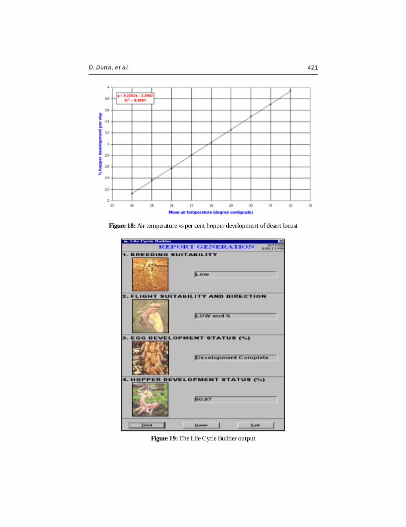
D. Dutta, et al. 421
Figure 18: Air temperature vs per cent hopper development of desert locust
Figure 19: The Life Cycle Builder output
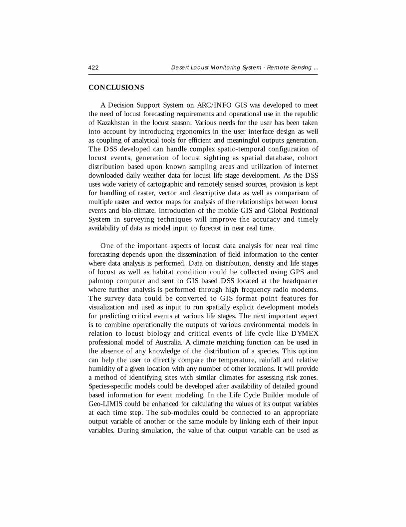
422 Desert Locust Monitoring System - Remote Sensing ...
CONCLUSIONS
A Decision Support System on ARC/INFO GIS was developed to meetthe need of locust forecasting requirements and operational use in the republicof Kazakhstan in the locust season. Various needs for the user has been takeninto account by introducing ergonomics in the user interface design as wellas coupling of analytical tools for efficient and meaningful outputs generation.The DSS developed can handle complex spatio-temporal configuration oflocust events, generation of locust sighting as spatial database, cohortdistribution based upon known sampling areas and utilization of internetdownloaded daily weather data for locust life stage development. As the DSSuses wide variety of cartographic and remotely sensed sources, provision is keptfor handling of raster, vector and descriptive data as well as comparison ofmultiple raster and vector maps for analysis of the relationships between locustevents and bio-climate. Introduction of the mobile GIS and Global PositionalSystem in surveying techniques will improve the accuracy and timelyavailability of data as model input to forecast in near real time.
One of the important aspects of locust data analysis for near real timeforecasting depends upon the dissemination of field information to the centerwhere data analysis is performed. Data on distribution, density and life stagesof locust as well as habitat condition could be collected using GPS andpalmtop computer and sent to GIS based DSS located at the headquarterwhere further analysis is performed through high frequency radio modems.The survey data could be converted to GIS format point features forvisualization and used as input to run spatially explicit development modelsfor predicting critical events at various life stages. The next important aspectis to combine operationally the outputs of various environmental models inrelation to locust biology and critical events of life cycle like DYMEXprofessional model of Australia. A climate matching function can be used inthe absence of any knowledge of the distribution of a species. This optioncan help the user to directly compare the temperature, rainfall and relativehumidity of a given location with any number of other locations. It will providea method of identifying sites with similar climates for assessing risk zones.Species-specific models could be developed after availability of detailed groundbased information for event modeling. In the Life Cycle Builder module ofGeo-LIMIS could be enhanced for calculating the values of its output variablesat each time step. The sub-modules could be connected to an appropriateoutput variable of another or the same module by linking each of their inputvariables. During simulation, the value of that output variable can be used as
D. Dutta, et al. 423
the input value. Scope is there that model designer can configure most modulesto adapt them for required task. Geo-LIMIS with little change in the inputlayers and habit suitability criteria interfaced with life stage builder specificto the species concerned could be used for modeling other exotic insect pestsand near real time forecasting for ground surveillance and control strategy.
ACKNOWLEDGEMENTS
The authors express their deep sense of gratitude to Dr K. Kasturirangan,Chairman, ISRO and Secretary, DOS, for his constant encouragement andguidance during this study. We are grateful to Shri V. Sundaramaiya, ScientificSecretary, ISRO for his guidance and support to bring out this manuscript.The authors are also thankful to the Director, Space Research Institute,Kazakhstan for extending support and valuable information for successfulcompletion of the project.
REFERENCES
Deveson, E.D. and Hunter, D.M. 2001. Decision Support for Australian Locust Managementusing Wireless Transfer of Field Survey Data and Automatic Internet Weather DataCollection (Unpublished).
FAO, 1989. Desert Locust Research Priorities. Report of the FAO Research Advisory Panel,2-5 May, 1989, Rome (FAO).
FAO, 1994. The Desert Locust Guidelines 1. Biology and Behavior, Rome.
Healey, R.G., Robertson, S.G., Magor, J.I., Pender, J. and Cressman, K. 1996. A GIS forDesert Locust Forecasting and Monitoring. Int. J. Geographical Information System,10 (1): 117-136.
http://pest.cpitt.uq.edu.au/forecast/intro.html.
http://www.environment.gov.au/land/monitoring/green.html.
Navathe, S. and Schkolnick, M. 1978. View Representation in logical database design. InProceedings of ACK-SIGMOD International Conference on Management of Data.Austin, TX. (ACM Press), pp. 144-156.
Pedgley, D.E. (editor) 1981. Desert Locust Forecasting Manual. Volume 1. (London:HMSO).
WORKSHOP EVALUATION
M.V.K. SivakumarWorld Meteorological Organization
7bis Avenue de la Paix, 1211 Geneva 2, Switzerland
INTRODUCTION
The Training Workshop (RA II) on Satellite Remote Sensing & GISApplications in Agricultural Meteorology, was co-sponsored by the WorldMeteorological Organization (WMO), the India Meteorological Department(IMD), the Centre for Space Science and Technology Education in Asia andthe Pacific (CSSTEAP), the Indian Institute of Remote Sensing (IIRS), theNational Remote Sensing Agency (NRSA) and the Space Applications Centre(SAC).
The Commission for Agricultural Meteorology (CAgM) of WMOrecognizes that training of technical personnel to acquire, process and interpretthe satellite imagery is a major task. This training workshop was organizedin response to the recommendations of the CAgM session in Ljubljana,Slovenia in 2002 with the objective of helping the participants from the Asiancountries in learning new skills and updating their current skills in satelliteremote sensing and GIS applications in agricultural meteorology.
Sixteen participants from thirteen Asian countries, including Bangladesh,China, India, Kazakhstan, Lao PDR, Maldives, Mongolia, Nepal, Saudi Arabia,Sri Lanka, Tajikistan, Thailand and the United Arab Emirates participated inthis training workshop.
FORMAT FOR THE TRAINING WORKSHOP
The training workshop was designed for agrometeorologists from Asia withlittle or no background in satellite remote sensing and GIS applications inagricultural meteorology.
The workshop started with a thorough introduction to various aspects ofsatellite and remote sensing along with practical exercises on the digital analysisof satellite data. This was followed by lectures on digital image processing,
Satellite Remote Sensing and GIS Applications in Agricultural Meteorologypp. 425-427

426 Workshop Evaluation
fundamentals of GIS and Geopositioning Systems (GPS) and spatial dataanalysis and practical demonstration of GIS software.
The participants were then introduced to both theoretical and practicalaspects of retrieval of agrometeorological parameters using satellite remotesensing data. This was followed by a lecture on remote sensing and GISapplication in agro-ecological zoning.
Remote sensing and GIS are very useful tools in crop growth andproductivity monitoring and simulation as well as assessment and monitoringof droughts, floods, water and wind induced soil erosion. Lectures were givenon all these aspects followed by practical demonstrations.
Participants were then introduced to satellite applications in weatherforecasting, agro-advisory services, desert locust monitoring, forest fire anddegradation assessment.
WORKSHOP EVALUATION
In order to facilitate the evaluation of the Seminar and help obtainfeedback from the participants, an evaluation form was circulated on the finalday. A summary of participant evaluation of the Seminar is shown in Table1. About 94% of the participants felt that the programme met the expressedobjectives of the workshop. The quality of the workshop programme was ratedby 100% of the participants as being very good to good. Sixty two percentof the participants rated the workshop as excellent while 19% rated it as verysuccessful.

M.V.K. Sivakumar 427