Remote sensing of tidal networks and their relation to vegetation Book or Report Section 

Accepted Version 

Mason, D.C. and Scott, T.R. (2004) Remote sensing of tidal networks and their relation to vegetation. In: Fagherazzi, S., Marani, M. and Blum , L. K. (eds.) The ecogeomorphology of tidal marshes. Coastal and estuarine studies (59). American Geophysical Union, pp. 27­46. ISBN 9780875902739 Available at http://centaur.reading.ac.uk/5846/ 

It is advisable to refer to the publisher’s version if you intend to cite from the work. 

Publisher: American Geophysical Union 

All outputs in CentAUR are protected by Intellectual Property Rights law, including copyright law. Copyright and IPR is retained by the creators or other copyright holders. Terms and conditions for use of this material are defined in the End User Agreement  . 

www.reading.ac.uk/centaur   

CentAUR 

Central Archive at the University of Reading 

Reading’s research outputs online

Remote Sensing of Tidal Networks and Their Relation to Vegetation

D. C. Mason and T. R. Scott

Abstract The study of the morphology of tidal networks and their relation to salt marsh vegetation is currently an active area of research, and a number of theories have been developed which require validation using extensive observations. Conventional methods of measuring networks and associated vegetation can be cumbersome and subjective. Recent advances in remote sensing techniques mean that these can now often reduce measurement effort whilst at the same time increasing measurement scale. The status of remote sensing of tidal networks and their relation to vegetation is reviewed. The measurement of network planforms and their associated variables is possible to sufficient resolution using digital aerial photography and airborne scanning laser altimetry (LiDAR), with LiDAR also being able to measure channel depths. A multi-level knowledge-based technique is described to extract networks from LiDAR in a semi-automated fashion. This allows objective and detailed geomorphological information on networks to be obtained over large areas of the inter-tidal zone. It is illustrated using LIDAR data of the River Ems, Germany, the Venice lagoon, and Carnforth Marsh, Morecambe Bay, UK. Examples of geomorphological variables of networks extracted from LiDAR data are given. Associated marsh vegetation can be classified into its component species using airborne hyperspectral and satellite multispectral data. Other potential applications of remote sensing for network studies include determining spatial relationships between networks and vegetation, measuring marsh platform vegetation roughness, in-channel velocities and sediment processes, studying salt pans, and for marsh restoration schemes.

Introduction

Tidal channel networks are integral features of the inter-tidal zone, and play a key role in tidal propagation, sediment transport and the evolution of tidal flats and salt marshes. To a large extent, these channels control the hydrodynamics of the tidal basin [Fagherazzi et al., 1999]. On ebb tides they drain the marshes and tidal flats, while on flood tides they act as conduits which the incoming water fills prior to flooding the areas around them. The sediment and nutrient exchanges between salt marshes and tidal flats and between tidal flats and the sea are also controlled through the network of tidal channels. A variety of network planform shapes exist [Pye and French, 1993]. On salt marshes the most common forms range in complexity from simple linear through linear-dendritic, dendritic, and meandering-dendritic to a complex form which may have basins at the heads of the lowest order channels deep in the marsh and wide higher order channels near its seaward edge. Channel dimensions range from several tens of metres wide and several metres deep near the low water mark to only about 30cm wide and 30cm deep for the smallest channels on the marshes. The lowest order channels tend to have width-to-depth ratios close to 1:1, while the highest order channels have larger values [Lawrence et al., in press]. Salt marsh channel cross-sections fall into a number of classes which depend on marsh type and tidal range, and channels may be V-shaped, U-shaped, rectangular-trapezoidal, roughly right-angled triangular, or with one or both banks overhanging [Allen, 2000]. Tidal channels on salt marshes influence the vegetation growing around them. A number of studies have noted that certain plants are associated with the sides of the channels, or grow on the small levees along the channels [e.g. Sanderson et al., 1998]. The levees are formed by sedimentation as flow velocity drops as bankfull is exceeded, and can be the sites of dense vegetation growth as the soil is well aerated and rich in nutrients. They also act as barriers for drainage from the marsh, and so can lead to waterlogged soil and thus reduced vegetation growth in the inner regions of the marsh [Carter, 1988]. In turn, the channels themselves are influenced by the vegetation. On tidal flats, channel movements may be quite rapid due to the lack of

vegetation, but within the marsh they are generally much slower, due in part to the binding and strengthening role played by the plant roots [Allen, 2000]. The processes governing network development and evolution are currently an open question. A number of geomorphological facts have been established and theories proposed. Early studies of channel geometry [Myrick and Leopold, 1963] and topology [Knighton et al., 1992] seemed to confirm their similarity to fluvial networks, and implied that they were formed by the draining of the tide from the marsh [French and Stoddart, 1992; Pye, 1992]. However, there are a number of important differences between the two network types. Tidal networks have a higher drainage density, though it is not clear what factors control this [Allen, 2000]. There are also differences in their topographies, in particular the catchment of a tidal network usually has a hydraulic boundary rather than a topographic one. The most important difference is the bi-directional flow which occurs in tidal channels [Steel, 1996]. Therefore others have postulated that they are not primarily drainage networks, but evolve due to the tidal and wave energy dissipated within them on the flood tide [Pethick, 1992]. Rinaldo et al. [1999a] found that parts of the network may be flood-dominated and others ebb-dominated. Unlike fluvial networks, tidal networks also have drainage densities which are not invariant across different scales [Rinaldo et al. 1999a, 1999b; Marani et al., in press]. Neither do they obey Hacks’ Law [Hacks, 1957] which, for fluvial channels, relates mainstream channel length to network watershed area over many scales. Marani et al. [submitted] have considered the geometric properties of tidal channels and shown that the ratio of the wavelength of channel meander to channel width remains remarkably constant across a range of scales. A model of channel initiation and evolution is also under development [Marani, 2003]. As regards channel equilibrium, Allen [2000] has proposed a theory to explain why salt marsh channel networks appear to be in dynamic equilibrium in the short term. Although over a period of months to years a channel may experience a large number of sedimentary events, these tend to cancel each other out so that the channel neither silts up nor erodes but maintains its cross-sectional area. According to the theory, if a salt marsh is in equilibrium, the square root of the integrated channel volume landward of a shore-parallel transect should be linearly related to the distance x of the transect from the shoreline. As regards the relationship between networks and vegetation, Sanderson et al. [2001] have developed a simple empirical model of salt marsh plant spatial distribution with respect to a tidal channel network. Extensive observational data of tidal channel networks and vegetation extracted from dense and accurate measurements over large areas of inter-tidal zone are required to substantiate these facts and validate these theories. A number of variables characterising tidal channels need to be measured. Many of these are encapsulated in the 2-D network planform. Knowledge of network planform allows many important variables of the network to be calculated, including channel lengths, widths, orders, bifurcation ratios, sinuousities and densities. To test other theories, depth-related variables such as cross-sectional areas and volumes are required. For marsh vegetation studies, different plant species assemblages need to be identified and their relationships with the marsh network system ascertained. The conventional method of measuring planforms and cross-sections of networks often involves network planforms being digitised manually from aerial photographs then amended by field survey. In addition field survey of channel cross-sections may be made for a selected subset of channels. Previous fieldwork on channel networks has concentrated on the network planform rather than on depth-related variables. Those field studies which do report cross-sectional areas do so for a small number of individual cross-sections, or at best total cross-sectional area over a number of transects [Lawrence et al., in press], rather than for the whole network. Examination of typical networks shows that these may have a density of 20km/km2 or more and that several square kilometres may need to be measured. The conventional technique, relying heavily on manual intervention, involves a great deal of effort and expense, is somewhat subjective, and can only acquire a limited set of field measurements. The same is true of most studies of the relationships between networks and marsh plant species distributions, which have generally been based on extensive field measurements. Allen [2000] has pointed out that one obstacle that has impeded progress towards understanding marsh systems is that their complexity has made it difficult for investigators to focus on the marsh as a whole. Recent advances in remote sensing

techniques mean that these can now often reduce measurement effort whilst at the same time substantially increasing measurement scale. The objectives of this paper are to review the current status of remote sensing of tidal networks and their relation to vegetation, to describe a technique which has been developed to extract channel networks from LiDAR data semi-automatically, and to consider possible ways in which remote sensing may advance understanding of tidal networks in the future.

The status of relevant remote sensing techniques

Which of these variables can be measured using remote sensing, either now or in the near future? Until recently, remote sensing resolutions were such that many of the smaller lower order channels could not be detected. This was particularly true of satellite remote sensing. However, resolutions continue to improve, and the Quickbird satellite now has a pixel size in panchromatic mode of only 70cm x 70cm, sufficient to image many though by no means all channels. Associated halophytic vegetation may also be classified into its constituent components with reasonable accuracy using the 4-band multispectral mode having a pixel size of 2.8m x 2.8m. However, in cases where a pixel contains a mixture of more than one class of vegetation, these multispectral data are unsuitable as they have too few spectral bands to allow unmixing techniques to be applied. An example applying unmixing techniques to multispectral Landsat imagery to extract relative amounts of vegetation, soil and water cover in order to determine marsh surface condition is given by Kearney et al. [2002]. The most important advance in remote sensing technology as far as this application is concerned has been in aerial remote sensing from aircraft or balloons. Digital colour cameras flown on aircraft can now achieve resolutions of 25cm, sufficient to image the smallest channels. Airborne hyperspectral sensors such as CASI (Compact Airborne Spectrographic Imager) and MIVIS (Multispectral Infrared and Visible Imaging Spectrometer), with resolutions up to 1m and ~100 spectral bands, can distinguish different salt marsh vegetation communities on the basis of their spectral signatures [Silvestri et al., 2003] (see Chapter 2a). Digital colour cameras mounted on balloons tethered several tens of metres above the marsh can achieve a resolution of 2cm, and can provide valuable temporal and spatial information regarding the sequence of events involved in marsh flooding and drying [Marani, pers. comm.]. A further important new data source for network detection is LiDAR [Gutelius, 1998; Baltsavias, 1999]. LiDAR is able to measure channel depths, cross-sections and volumes as well as network planform variables. A spatial resolution of 25cm or so is currently possible, coupled with a height accuracy of 15 cm, so that even the smallest channels may be detected. LiDAR is thus able to provide topographic data at a scale and height accuracy which matches that required for present-day geomorphological studies on networks. The current trend is to acquire LiDAR in conjunction with colour aerial photography or multispectral linescanner data to provide the user with a visual image of the LiDAR DEM. It is true that LiDAR can only measure channel cross-sections if channels are completely drained, and may underestimate cross-sectional areas in channels containing overhangs, but it nevertheless remains an important new data source for this application. LiDAR is also an evolving technology and future improvements are to be expected. There are thus several areas in which remote sensing can benefit the study of tidal networks. These include measurement of network planforms and associated variables to the necessary resolution using aerial photography and LiDAR, with LiDAR also being able to measure channel depths and their dependent variables. Associated marsh vegetation can be classified into its component species using airborne hyperspectral and (with lower accuracy) satellite multispectral data. Other potential uses of remote sensing include determining spatial relationships between networks and vegetation using GIS techniques; use of LiDAR for the calibration of hydrodynamic models for studying water flows in the channels and over the marsh; measurement of in-channel water velocities using airborne interferometric synthetic aperture radar (InSAR); measurement of sediment processes within channels; measurement of salt pans; and marsh restoration planning and monitoring. These are considered in the following sections.

Semi-automated network extraction from LiDAR and aerial photography/linescanner data The digital data acquired by remote sensors can also make possible more automated measurement of network variables. Extraction of networks can be performed manually or by using an automated image processing algorithm. Advantages of using image processing are the low cost of analysing the images compared to manual methods, and the consistent approach that is used. Disadvantages are the initial effort of developing the algorithm, and the fact that automatic extraction is unlikely to be as accurate as manual, suffering from errors of omission where channels are not detected and errors of commission where other features are incorrectly identified as channels. Channel networks are complex natural scenes and it is extremely difficult to devise an algorithm that will work correctly in all situations. This section describes a semi-automatic technique that has been developed to extract networks from LiDAR data [Mason et al., submitted]. The method is termed semi-automatic because at various points in the procedure the human operator is called upon for assistance, including the correction of errors in the final output. In the future it is hoped to extend the technique to use aerial photography instead of LiDAR data, or both LiDAR and aerial photography combined in a fusion approach which should produce an improved channel network. Aerial photographs of intertidal zones are presently much more commonly available than LiDAR data, and are particularly useful for providing a snapshot of a marsh in the (pre-LiDAR) past for comparison with its present-day state. The method is an example of drainage network extraction from a digital elevation model (DEM). There has been extensive research into the development of techniques for extracting river channel networks from low resolution terrestrial DEMs. Examples are the steepest gradient method of Jenson and Domingue [1988] and the multilevel skeletonisation technique of Meisels et al. [1995]. The performance of these methods has been shown to be only moderate when applied to LiDAR imagery of tidal channels, due to the different morphological characteristics of fluvial and tidal channels and the very high spatial resolution of LiDAR [Lohani and Mason, 2001]. The first attempt at a method of automatic channel network extraction was made by Fagherazzi et al. [1999], using a low resolution (non-LiDAR) DEM and a method based on elevation and curvature thresholds rather than hydrological properties which worked well for the larger channels. A multi-level knowledge-based approach has been implemented, whereby low level algorithms first extract channel fragments based mainly on image properties then a high level processing stage repairs breaks in the network using domain knowledge. A full description of the method is given in [Mason et al., submitted] and only a summary is presented here. The channels exhibit a width variation of several orders of magnitude, making an approach based on multi-scale line detection difficult. The low level algorithm therefore uses edge detection to detect channel edges, then associates adjacent parallel edges together to form channels. This has the advantage that the low level processing can be made similar for LiDAR and aerial photographs. The various steps in the procedure are illustrated below using a 1km x 1km LiDAR image of the River Ems, Germany (figure 1). The Ems estuary is an example of unvegetated tidal flats in a macrotidal area. TopoSys data of the Ems were acquired at low water in last-return mode at a flying height of 850m and a flying speed of about 70ms-1. The laser wavelength was 1.54 µm, laser pulse rate 83kHz, scan half-angle 7º, scan rate 630 Hz and laser footprint 0.3m [Baltsavias, 1999]. The mean measurement point density was about 4/m2, which was reduced by an averaging process to a final pixel size of 1m x 1m. The image exhibits a number of tidal channels and shows their width variations, though a crude sea-wall and ditch structure has unfortunately been constructed across the bottom of the area. The height range in the image is 2.8m.

Figure 1 here

Low level processing

Low level processing consists of pre-processing, edge detection and edge association. A number of pre-processing steps are applied to the data, including interpolation across small gaps (e.g. between adjacent flight swaths), and use of a Laplacian filter to suppress small regions significantly higher than the local mean

height. Where salt marshes are present in the inter-tidal zone, the LiDAR returns may contain signals due to short vegetation generally less than 1m high. The objective is to search for linear channels in the underlying ground DEM rather than the Digital Surface Model (DSM) acquired by the LiDAR. It would be possible to remove vegetation heights from the DSM, for example using local LiDAR height texture to estimate vegetation height [Cobby et al., 2001]. However, our experiments show that noise due to vegetation can be limited simply by raising edge thresholds. In contrast to the channel width variation of several orders of magnitude, the variation in the slopes at the channel banks spans a narrower range. The majority of the edges of the smaller channels in the salt marsh and upper tidal flats can be detected using a high frequency (HF) edge detector, though those of larger channels near the low water mark can only be detected using a low frequency (LF) detector. A two-scale edge detector comprising separate HF and LF edge operators is therefore used for channel edge detection. In combining the edges of different scales at a given pixel, the smaller HF edge is used provided that it is sufficiently strong, since this gives the best localization of the edge (figure 2a). Edges which are non-maxima along an axis perpendicular to their edge direction are then suppressed. Edge maxima lying within the larger channels are also suppressed. Surviving edge maxima are then thresholded using hysteresis thresholding and thinned to single pixel width (figure 2b). Hysteresis thresholding helps to fill in gaps of lower edge strength pixels between runs of higher edge strength pixels, giving a more continuous edge. Edge detection of a tidal channel will generate two anti-parallel edges from either side of it. These must be associated together. This is achieved by generating the distance transform of the edge image, in which a pixel’s value is its distance from the nearest edge, with distances being zero at edge pixels (figure 2c). The transform is operated upon to identify positions having distances that are maxima or saddle points, by performing non-maximum suppression followed by thinning (figure 2d). The distance maxima occur at the centrelines of channels, but other maxima of no interest will occur between channels. To differentiate between these two classes of maxima, a score is calculated for each maximum based on the thresholded edge and LiDAR height images. A distance maximum’s score is big if it is linked with perfectly anti-parallel edges with a narrow separation bounding runs of pixels with heights less than the edge heights, and with heights increasing away from the channel centre. Long connected strings of pixels having high scores are then selected using hysteresis thresholding (figure 2e). Figure 2 here High level processing

The high level processing consists of a network repair stage and a channel expansion stage. At this stage the thresholded score image consists of sets of channel network centrelines with each network consisting of a number of disconnected fragments. Breaks in the networks are repaired by extending channel ends in the direction of their ends to join with nearby channels. For each endpoint, a search for a channel centreline pixel to join with is made by searching forward in a triangle with its apex at the endpoint being considered, and oriented in the direction of the endpoint . The repair procedure has two stages. In the first stage, a search triangle with a large base-to-height ratio is used to join centreline pixels that are relatively close to the endpoint (irrespective of whether they are upstream or downstream of the endpoint). In the second stage, longer more directed joins are attempted using a longer triangle with a small base-to-height ratio. Domain knowledge is used at this stage, namely that flow paths should proceed downhill, and candidate centreline pixels must be lower than the endpoint to be joined with. For each candidate centreline pixel in the search triangle, the optimum path along which to join candidate and endpoint is determined using a local weighted distance-with-destination transform in which higher pixels are assigned larger distance increments [Mason et al., submitted; Lohani and Mason, 2001]. The path associated with the minimum weighted distance is identified within this. After all valid candidate centreline pixels in the current search triangle have been examined, the candidate with the minimum weighted distance is chosen, and the endpoint is joined with its centreline pixel along the minimum path. This procedure is repeated for all endpoints in the image.

Connected network regions are then found in the repaired score image, with small regions being rejected. A confidence is calculated for each network based on the sum of the scores of all pixels making up its region, and networks having very low confidences are rejected. The repaired channel centrelines are shown in figure 2f. After the repair stage, a binary image of the channels may be constructed by selecting all pixels between each distance maximum and its associated edges. However, in order to test geomorphological theories, channel volumes and cross-sections need to be calculated when channels are at bankfull. The waterline positions at bankfull extent may be defined as coinciding with the positions of maximum negative curvature in the channel, which in general will lie above the positions of maximum edge strength, so that the channels extracted so far will be too narrow. A final stage therefore expands the current channels to their bankfull extents by estimating, at each pixel on the channel boundary, an approximate position for the maximum of negative curvature from the position of maximum edge strength. To do this, the local mean background height just outside the channel is calculated, and is used with the edge strength (figure 2a) to calculate an expansion distance at that pixel. The expansion distance is smoothed using the expansion distances of the neighbouring edge pixels. The background heights are also interpolated over the channels so that channel cross-sections and volumes can be calculated.

Results

Figure 3 shows the bankfull channel outlines superimposed on the original LiDAR heights. These were compared quantitatively with the results of manual digitisation of the channels. Channels proved to be not always easy for the operator to define. They may have a bank that is higher on one side than the other, there may be channels within channels, and they may merge into salt pan areas. In these cases a guiding principle used for distinguishing the channel boundaries was that in a channel the water should have a predominantly 1-D rather than 2-D flow associated with it. The error of commission of the automatic channel extractor was found to be low, and the error of omission reasonably low (table 1). The main defect found was that numerous small channels visible to the eye in the LiDAR data were lost because they fell below the edge threshold. However, these were less than 10cm deep. A fact noted at this stage was how tedious and slow it was to perform the manual digitisation.

Figure 3 and Table 1 here

The method has also been applied to LiDAR data of other regions which differ hydrodynamically, geomorphologically and ecologically from the River Ems. Figure 4 shows TopoSys LiDAR data of the San Felice area, Venice Lagoon, covering 0.5 x 0.5 km. These data, acquired at low water at a flight altitude of 500m, have a pixel size of only 50cm x 50cm, so that the majority of the channels are resolved. The height range in the image is –0.1m a.m.s.l to +0.7m a.m.s.l. The area is composed mainly of salt marsh covered by short vegetation less than 50cm high. The ability of LiDAR to distinguish the levees adjacent to the channels is clearly evident. Figure 4 also shows the bankfull channel outlines detected by the automatic procedure. While the error of omission was low, there was a significant error of commission (42%), due partly to the confusing situation in the NW of the image (table 1). Here the channel structure becomes ambiguous, consisting of shallow depressions and salt pans which the automatic procedure identified as channels while the operator did not. The method was also applied to Optech LiDAR data of Carnforth Marsh, Morecambe Bay, UK, which is covered with patches of taller vegetation up to 1m high. It was found that 1m-high vegetation raises the local mean heights only by 10-15cm, due to the majority of the returns emanating from surfaces below the top of the canopy, and that noise from this source could be limited simply by raising edge thresholds.

Figure 4 here Examples of geomorphological variables of networks extracted from LiDAR data

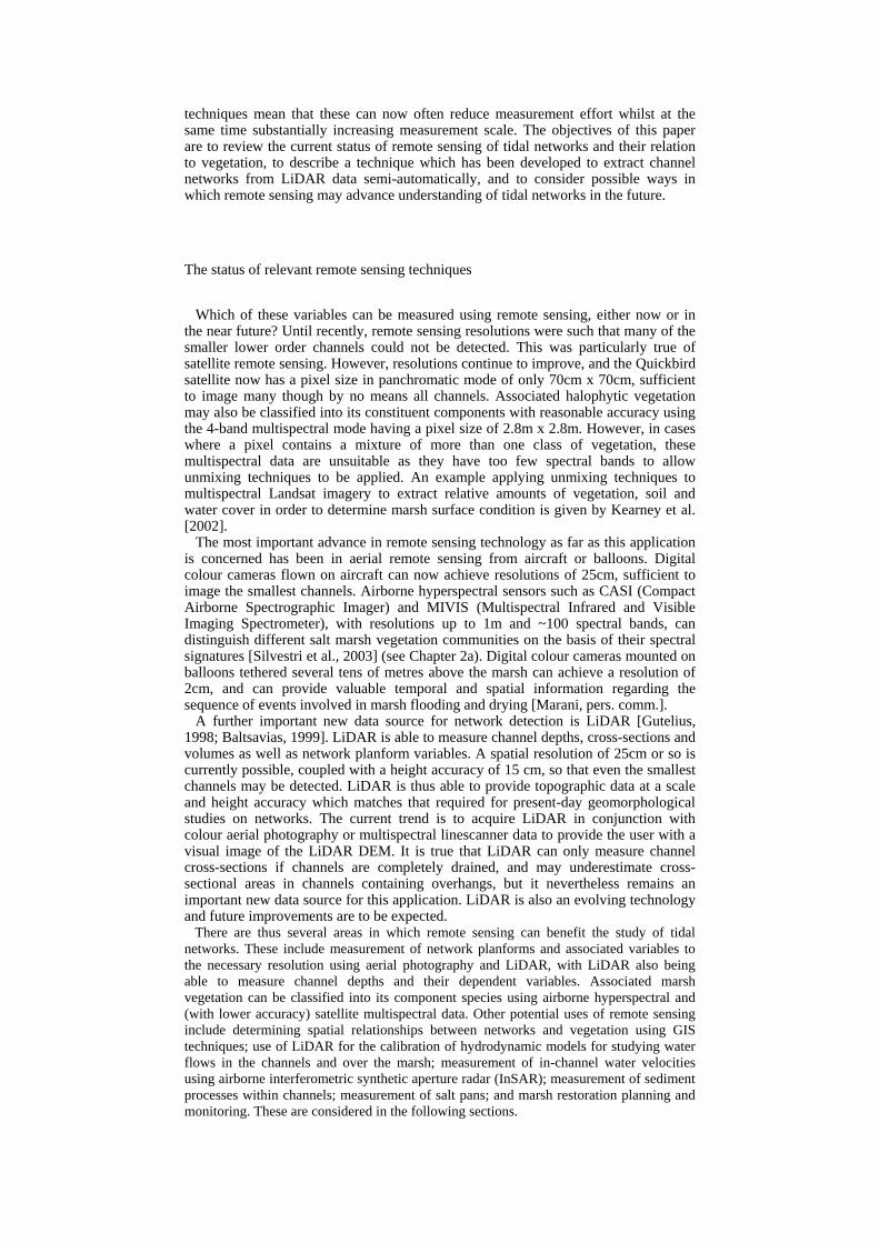
This section gives examples of network planform and volume variables extracted from LiDAR data. The first example, taken from [Lohani and Mason, 2001], is of drainage densities for a network in the River Ems LiDAR data (figure 5a). Drainage density is an important parameter describing the degree of dissection of terrain by surface streams and is defined as the ratio of the total drainage length Ls to the watershed area A. The drainage density for fluvial networks is constant over a wide

range of scales [Rinaldo et al., 1999a]. The measurements of Ls and A were determined for each possible channel cross-section and its associated watershed in the network using an automatic technique based on the concept developed by Rinaldo et al. [1999b] for locating watershed boundaries in a tidal basin. To ensure proper connectivity of the network and the removal of noise, it was corrected manually for errors of omission and commission. The plot of drainage density versus watershed area is shown in figure 5b. A point on the plot represents the relationship between drainage density and watershed area for a cross-section (i.e. a point on the channel skeleton) of the network. Though the basic purpose of the plot is to show the relationship between drainage density and watershed area over several scales, the colour annotation helps to identify this relationship for different parts of the network. The plot shows that the drainage density versus watershed area relationship changes within the network (the colour of a network section in figure 5a identifies its relationship in figure 5b). This observation corroborates the results obtained by Rinaldo et al. [1999b] that drainage density in a tidal environment is scale-dependent and does not show the scale-independent relationship found for fluvial networks.

Figure 5 here

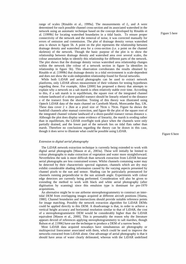
While both LiDAR and aerial photographs can be used to extract network planforms, only LiDAR allows measurement of their volumes for testing hypotheses regarding these. For example, Allen [2000] has proposed a theory that attempts to explain why a network on a salt marsh is often relatively stable over time. According to this, if a salt marsh is in equilibrium, the square root of the integrated channel volume landward of a shore-parallel transect should be linearly related to the distance x of the transect from the shoreline. Testing of this theory was illustrated using Optech LiDAR data of the main channel on Carnforth Marsh, Morecambe Bay, UK. These data cover 2 x 2km at a pixel size of 70cm x 70cm. Figure 6a shows the bankfull channels after manual correction, and figure 6b the plot of the square root of the integrated channel volume landward of a shore-parallel transect versus distance x. Although the plot does display some evidence of linearity, the marsh is eroding rather than in equilibrium, the LiDAR overflight took place when the channels were only partially drained, and the lower part of the network lies on tidal flats rather than marsh. Therefore no conclusions regarding the theory can be drawn in this case, though it does serve to illustrate what could be possible using LiDAR.

Figure 6 here Extension to digital aerial photography

The LiDAR network extraction technique is currently being extended to work with digital aerial photographs [Mason et al., 2003a]. These will initially be limited to colour photographs to make extraction of vegetation and water more straightforward. Nevertheless the task is more difficult than network extraction from LiDAR because aerial photographs are less constrained scenes. Whilst channels containing water may be detected by their characteristic spectral signature, channels which are dry may exhibit considerable shading information caused by the varying aspects presented by channel pixels to the sun and sensor. Shading can be particularly pronounced for channels running perpendicular to the sun azimuth angle. Experiments with colour edge detectors are currently being performed. Consideration will also be given to extending the method to work with black and white aerial photography (after digitisation by scanning) since this emulsion type is dominant for pre-1970 acquisitions. An alternative might be to use airborne stereophotogrammetry to construct an inter-tidal DEM from overlapping images acquired at different aircraft positions [Slama, 1980]. Channel boundaries and intersections should provide suitable reference points for image matching. Possibly the network extraction algorithm for LiDAR DEMs could be applied directly to this DEM. A disadvantage is that, in order to achieve a vertical height accuracy and horizontal resolution similar to that of LiDAR, the cost of a stereophotogrammetric DEM would be considerably higher than the LiDAR equivalent [Mason et al., 2000]. This is presumably the reason why the literature appears devoid of references applying stereophotogrammetry to salt marshes, though Balson et al. [1996] have use the technique to produce a DEM of a narrow beach. Most LiDAR data acquired nowadays have simultaneous air photography or multispectral linescanner associated with them, which could be used to improve the networks extracted from LiDAR alone. One advantage of aerial photography is that it should have areas of water clearly delineated, whereas with the LiDAR undefined

areas may be either water or outside the LiDAR coverage. Fusion of edges in the two edge sets detected separately in aerial photographs and LiDAR data is being considered. Further potential uses of remote sensing for network studies

There are a number of other ways in which remote sensing might be used for network studies. Some of the more important are discussed below. Determination of spatial relationships between networks and vegetation

Up to now the only relationship between tidal channels and salt marsh vegetation considered has been the effect of vegetation height changes on the edge threshold in the channel extraction algorithm. A more obvious use for remote sensing would be to ascertain whether any spatial relationships between vegetation and tidal channels exist, such as whether particular vegetation types are predominant near the channels. Sanderson et al. [2000] found that tidal channels did indeed influence the distribution and composition of vegetation in a San Francisco salt marsh. Using field measurement and GIS techniques, they found that composition of plant species assemblages varied with distance from the channel banks and with channel size. The generality of this finding could be tested using remote sensing by repeating this type of study at a larger scale over a variety of marshes. A map of vegetation type could be obtained by airborne remote sensing using the classification techniques described in Chapter 2a. This could be overlain with a map of channel networks derived from LiDAR or aerial photography, and spatial relationships determined using a GIS. Similarly, a recent remote sensing study [Sanderson et al., 1998] using low resolution satellite data of the same San Francisco marsh showed that the tidal channels have an important influence on the patterns of canopy water content across the marsh landscape, even for very small channels. Again, this result could be tested for generality at higher resolution for this marsh and others using airborne remote sensing.

Use of LiDAR data for hydrodynamic model calibration

A more subtle use of remote sensing would be to use LiDAR data to calibrate a hydrodynamic model used for studying water flows in the channels and over the marsh. Lawrence et al. [in press] have used a 2-D depth-averaged hydrodynamic model to investigate tidal flows over an idealised marsh. The authors show that roughness due to marsh platform vegetation exerts a significant influence on the partitioning of water flow between the channel network and the seaward edge of the marsh, alters flow patterns on the marsh platform due to its effects on channel-to-platform transfer and also controls the timing of peak discharge relative to marsh-edge overtopping. A global value of Manning’s n appropriate to flows over vegetated floodplains was used to represent salt marsh surface roughness. For modelling flows over real marshes, LiDAR data can provide marsh ground topography for use as model bathymetry, and also vegetation heights, which can be used to estimate surface friction coefficients. This approach has the advantage that modelling results become independent of assumptions regarding the magnitude and spatial uniformity of Manning’s n. Mason et al. [2003b] studied friction parameterisation of rural floodplains in 2-D river flood models, using LiDAR-derived vegetation heights to estimate a spatially-distributed friction parameterisation. Local vegetation height was estimated using the local standard deviation of LiDAR-derived heights after de-trending to remove low frequency height changes. The standard deviation was low for short floodplain vegetation such as grasses and crops, but larger for taller vegetation such as woodland and hedges. For short vegetation up to 1.2m high, vegetation height could be estimated to ±14 cm accuracy. A set of empirical equations was used to derive Manning’s n given vegetation height, water depth and flow velocity. These equations took into account the fact that the vegetation may change from being emergent to submerged as water depth gradually increases, and that submerged vegetation may bend in the flow, resulting in a reduction in friction.

The equations reflect the findings of Wu et al [1999], who found by experiment that the friction factor of an emergent vegetation canopy gradually reduced with increasing flow depth up to a point at which the canopy became submerged. After submergence, friction initially increased slightly with increasing water depth, then fell substantially as water levels increased further. Such hydrodynamic model calibration could probably be improved using complementary knowledge of vegetation type acquired by multi- or hyperspectral remote sensing. Measurement of in-channel velocities

Another possibility is that remote sensing could be used to measure water velocities within the channels. Channel velocities are low (0.1 – 0.2ms-1) while water levels are below but not too close to bankfull, but rise significantly to up to 1ms-1 or more at levels above bankfull when channel capacity is exceeded and the large storage capacity of the marsh comes into play [Allen, 2000]. The ebb flow in a channel is generally stronger and peaks at a slightly lower stage than the flood. Current evidence is that bankfull velocity in a network is virtually uniform throughout the network. For example, Rinaldo et al. [1999a], in their studies of Venice Lagoon marshes, found that peak channel velocity was spatially constant. Stoddart et al. [1987] have also studied the spatial variability of velocities on a salt marsh on the Wash. The theory of marsh channel equilibrium due to Allen [2000] is based on the assumption that the velocities along a channel network are spatially uniform. To date, velocity measurements have been made only at selected channel locations in a marsh. Remote sensing could be used to test this theory in a more synoptic fashion. This should be possible using an airborne synthetic aperture radar (SAR) with an along-track interferometric capability, at least for channels wider than about 5m. The basic idea of along-track interferometery is that the motion of the Bragg scatterers due to currents in the water surface causes a phase difference in the signals received at the plane's two antennae, and that this phase difference is a function of the surface current component towards the radar. As the surface velocity may also have a component due to surface wind drift, it is important to carry out measurements at low wind speeds. Two orthogonal flight lines are needed to measure the velocity vector [Frasier and Camps, 2001]. Previous studies on river channels [Costa et al., 2000] have shown that it is possible to relate the surface current in the channel to the depth-averaged current through a simple current profile model, given knowledge of channel bathymetry obtained using LiDAR. Surface velocity accuracies of 0.1ms-1 are quoted for the method, sufficient to measure meaningful velocities when water levels are close to bankfull or above.

Measurement of sediment processes within channels

A natural extension of the above is the use of remote sensing to measure sediment transport within channel networks. If sediment concentrations in channels could be measured using high resolution sensors, these could be combined with channel dimensions and channel velocity profiles to provide sediment transport rates. Allen [2000] has pointed out that the movement of water and sediment across a marsh platform interrupted by channels is the key to its topography, yet remains perhaps the worst understood aspect of marsh morphodynamics. A number of studies have used remote sensing for mapping suspended sediments in coastal waters [e.g. Aguirre-Gomez, 2000; Jorgensen and Edelvang, 2000]. In the latter study, a CASI sensor, capable of a resolution as low as 1m, was used to map suspended sediment concentrations in a sediment plume. The suspended sediment concentration was derived using an empirical algorithm depending on in situ irradiance reflectance at 550nm and suspended matter concentrations determined from water samples taken both inside and outside the plume. Measurement of the spatial pattern of accretion rates over the marsh surface are also required [e.g. French and Spencer, 1993], and could be used in conjunction with sediment transport rates to validate sediment transport models of the marsh system. Unfortunately accretion rates are generally on the order of only 1cm per year, so that a substantial time would need to elapse before accretion rates measured by LiDAR could be deemed to be significantly non-zero, given the height error associated with

LiDAR. A related possibility is the monitoring and measurement of regions of channel bank collapse using LiDAR and digital photography. Bank collapse is a mechanism for returning sediment to suspension and redistributing it over the marsh, and can be an important source of sediment. Thus a marsh may increase in height more rapidly if the banks are less stable. Measurement of salt pans

Remote sensing may perhaps also be used to study salt pans on marshes. These are hollows which often contain standing water of high salinity left after evaporation, and are usually only colonised by species tolerant of high salinity. The main mechanism by which these form is still unclear [Carter, 1988]. One possibility is that in smaller channels bank collapses or gradual sedimentation can infill the channel, cutting off the head of the channel and creating a pool. The presence of salt pans at the heads of lower order channels may be indicative of a mature marsh undergoing erosion [Allen, 2000]. However, other mechanisms are also possible. The number of pans is known to be more numerous as the marsh rises and to increase towards the seaward margin of the marsh [Pethick, 1974]. Airborne remote sensing could be used to investigate whether salt pans may once have been part of a channel or have arisen by other means, and to determine their distribution within a marsh. Infrared sensors could also be used to measure the temperature of the water in the pans. Van Huissteden and Van de Plassche [1998] have hypothesized that degradation of organic matter by sulphate-reducing bacteria in peat-rich marsh deposits is the primary cause of pan formation, and that sulphate reduction is probably enhanced by higher pan water temperatures. To test their theory, they suggest that more thorough measurement of temperature variations within the pans and surrounding peat be made. Marsh restoration planning and monitoring

Characteristics of mature and stable marshes, calculated from LiDAR data, could be used for marsh restoration projects. A number of studies [e.g. Zeff, 1999] have demonstrated the need to mimic the natural drainage system of local marshes in the design of new channel systems at restoration sites. Zeff [1999] advocates that the networks in restored marshes should reflect the geometry and depth patterns (width/depth ratios, cross-sectional areas, longitudinal slopes, hydraulic geometry) found in similar natural systems. This procedure should render the restored marsh more stable, make it colonisable by vegetation more rapidly, and reduce the practice of excavating larger channels than are necessary, which leads to higher construction and sediment disposal costs.

Conclusion

Airborne digital cameras and hyperspectral scanners are now able to provide data at a spatial resolution and precision matching that required for network planform and vegetation studies. Airborne LiDAR can provide topographic data at sufficient vertical and horizontal resolution for network planform and volume studies, and is amenable to automatic network extraction techniques. The semi-automatic technique described here allows objective and detailed geomorphological information on networks to be obtained from LiDAR data over large areas of the inter-tidal zone. Remote sensing also has potential for measurement of marsh platform vegetation roughness, in-channel velocities and sediment processes, and also for salt pan studies and marsh restoration schemes. Due to its synoptic capability and relatively low cost, increasing use of remote sensing for network studies is likely in the future. Acknowledgement. This work was funded under the EU FP5 project TIDE (Tidal Inlet Dynamics and Environment) (EVK3-CT-2001-00064). Thanks are due to TopoSys, Germany and

the UK Environment Agency for provision of the LiDAR data, and to the anonymous referees whose suggestions improved the manuscript.

References

Aguirre-Gomez, R., Detection of total suspended sediments in the North Sea using AVHRR and ship data. Int. J. Remote Sensing, 21, 1583-1596, 2000. Allen, J. R. L., Morphodynamics of Holocene salt marshes: a review sketch from the Atlantic and southern North Sea coasts of Europe. Quaternary Science Reviews, 19, 1155-1231, 2000. Balson, P. S., D. G. Tragheim, A. M. Denniss, D. Waldram and M. J. Smith, A photogrammetric technique to determine the potential sediment yield from recession of the Holderness coast, UK, in Partnership in Coastal Zone Management, edited by J. Taussik and J. Mitchell, pp. 507-514, Samara Publishing Ltd., Cardigan, UK, 1996. Baltsavias, E. P., Airborne laser scanning systems: existing systems and firms and other resources. ISPRS Journal of Photogrammetry and Remote Sensing 54, 164-198, 1999. Carter, R. W. G., Coastal environments; an introduction to the physical, ecological and cultural systems of coastlines, Academic Press, London, 1988. Cobby, D. M., D. C. Mason and I. J. Davenport, Image processing of airborne scanning laser altimetry data for improved river flood modelling. ISPRS J. Photogrammetry and Remote Sensing, 56, 121-138, 2001. Costa J. E., K. R. Spicer, R. T. Cheng, F. P. Haeni, N. B. Melcher, E. M. Thurman, W. J. Plant and W. C. Keller, Measuring stream discharge by non-contact methods: a proof-of-concept experiment. Geophys. Res. Lett., 27, 553-556, 2000. Fagherazzi, S., A. Bortoluzzi, W. E. Dietrich, I. Rodriguez-Iturbe, A. Adami, S. Lanzoni, M. Marani and A. Rinaldo, Tidal networks 1: automatic network extraction and some scaling features from DTMs. Water Resources Research, 35, 3891-3904, 1999. Frasier S. J. and A. J. Camps, Dual-beam interferometry for ocean surface current vector mapping. IEEE. Trans. Geo. Rem. Sens., 39, 401-414, 2001. French, J. R. and D.R. Stoddart, Hydrodynamics of salt marsh creek systems – implications for marsh morphological development and material exchange. Earth Surface Processes and Landforms, 17, 235-252, 1992. French, J. R. and T. Spencer, Dynamics of sedimentation in a tide-dominated backbarrrier salt marsh, Norfolk, UK. Marine Geology, 110, 315-331, 1993. Gutelius, B., Engineering applications of airborne scanning lasers: reports from the field. Photogrammetric Engineering and Remote Sensing, 64, 246-53, 1998. Hacks, J.T., Studies of longitudinal profiles in Virginia and Maryland, U.S. Geological Survey Professional Paper, 294-B, 1957. Jenson, S. K. and J. O. Domingue, Extracting topographic structure from digital elevation data for geographic information system analysis. Photogrammetric Engineering and Remote Sensing, 54 , 1593-1600, 1988. Jorgensen, P. V. and K. Edelvang, CASI data utilized for mapping suspended matter concentrations in sediment plumes and verification of 2-D hydrodynamic modelling. Int. J. Remote Sensing, 21, 2247-2258, 2000. Kearney, M. S., A. S. Rogers, J. R. G. Townshend, E. Rizzo, D. Stutzer, J. Court Stevenson and K. Sundborg, Landsat imagery shows decline of coastal marshes in Chesapeake and Delaware Bays. EOS Transactions, 83, 173-178, 2002. Knighton, A.D., D.C. Woodruff and K. Mills, The evolution of tidal creek networks, Mary River, Northern Australia. Earth Surface Processes and Landforms, 17, 167-190, 1992. Lawrence, D. S. L., J. R. L. Allen and G. M. Havelock, Salt marsh morphodynamics: an investigation of tidal flows and marsh channel equilibrium. Journal of Coastal Research, 19, in press. Lohani, B. and D. C. Mason, Application of airborne scanning laser altimetry to the study of tidal channel geomorphology. ISPRS J. Photogrammetry and Remote Sensing, 56, 100-120, 2001. Marani, M., S. Lanzoni, D. Zandolin, G. Seminara and A. Rinaldo, Tidal meanders, Water Resources Research, 38(11), 1225-1239, 2002. Marani, M., A. Belluco, A. D’Alpaos, A. Defina, S. Lanzoni and A. Rinaldo, The drainage density of tidal networks, Water Resources Research, 39(2), 1040, doi:10.1029/2001WR001051, 2003. Marani, M., Development of model of tidal systems evolution. TIDE Periodic Report, Feb. 2002 – Jan. 2003, 2003. Mason, D. C., C. Gurney and M. Kennett, Beach topography mapping – a comparison of techniques. Journal of Coastal Conservation, 6, 113-124, 2000. Mason, D. C., H-J. Wang and B. Lohani, Extraction of tidal channel networks from airborne scanning laser altimetry and aerial photography. Proc. EOS/SPIE Symp. on Image Processing for Remote Sensing VIII, Crete, Sept. 2002, 8pp, 2003a. Mason D. C., D. M. Cobby, M. S. Horritt and P. Bates, Floodplain friction parameterisation in two-dimensional river flood models using vegetation heights derived from airborne scanning laser altimetry. Hydrological Processes, 17, 1711-1723, 2003b. Mason, D. C., T. R. Scott and H-J. Wang, Extraction of tidal channel networks from airborne scanning laser altimetry. ISPRS J. Photogrammetry and Remote Sensing, submitted. Meisels, A., S. Raizman and K. Arnon, Skeletonizing a DEM into a drainage network. Computers and Geosciences 21(1), 187-196, 1995. Myrick, R. M. and L. B. Leopold, Hydraulic geometry of a small tidal estuary. U.S. Geological

Survey Professional Paper 422-B, 1-18, 1963. Pethick, J. S., The distribution of salt pans on tidal salt marshes. Journal of Biogeography, 1, 57-62, 1974. Pethick, J.S., Saltmarsh geomorphology, in Saltmarshes: Morphodynamics, Conservational and Engineering Significance, edited by J. R. L. Allen and K. Pye, Cambridge University Press, Cambridge, 148-178, 1992. Pye, K., Saltmarshes on the barrier coastline of North Norfolk, eastern England, in Saltmarshes: Morphodynamics, Conservational and Engineering Significance, edited by J. R. L. Allen and K. Pye, Cambridge University Press, Cambridge, 148-178, 1992. Pye, K. and J. R. French, Erosion and accretion processes on British salt marshes. Vol. 1, Introduction: Saltmarsh Processes and Morphology, Cambridge Environmental Research Consultants, Cambridge, 1993. Rinaldo, A., S. Fagherazzi, S. Lanzoni, M. Marani and W. E. Dietrich, Tidal networks 3. Landscape-forming discharges and studies in empirical geomorphic relationships. Water Resources Research, 35, 3919-3929, 1999a. Rinaldo, A., S. Fagherazzi, S. Lanzoni, M. Marani and W. E. Dietrich, Tidal networks 2. Watershed delineation and comparative network morphology. Water Resources Research, 35, 3905-3917, 1999b. Sanderson, E. W., M. Zhang, S. L. Ustin and E. Rejmankova, Geostatistical scaling of canopy water content in a California salt marsh. Landscape Ecology, 13, 79-92, 1998. Sanderson, E. W., S. L. Ustin and T. C. Foin, The influence of tidal channels on the distribution of salt marsh plant species in Petaluma Marsh, CA, USA. Plant ecology, 146, 29-41, 2000. Sanderson, E. W., T. C. Foin and S. L. Ustin, A simple empirical model of salt marsh plant spatial distributions with respect to a tidal channel network. Ecological modelling, 139, 293-307, 2001. Silvestri, S., M. Marani and A. Marani, Hyperspectral remote sensing of salt marsh vegetation, morphology and soil topography. Physics and Chemistry of the Earth, 28, 15-25, 2003. Slama, C., Manual of Photogrammetry, American Society of Photogrammetry, Falls Church, VA, 1980. Steel, T.J., The morphology and development of representative British saltmarsh creek networks. Ph.D. Thesis, Postgraduate Research Institute for Sedimentology, The University of Reading, 1996. Stoddart, D. R., J. R. French, T. P. Bayliss-Smith and J. Raper, Physical processes on Wash salt marshes, in The Wash and its Environment, edited by P. Doody and B. Barnett, 64-76, Nature Conservancy Council, Peterborough, UK, 1987. Van Huissteden, J. and O. Van de Plassche, Sulphate reduction as a geomorphological agent in tidal marshes (‘Great Marshes’ at Barnstable, Cape Cod, USA). Earth Surface Processes and Landforms, 23, 223-236, 1998. Wu F-C., H. S. Shen and Y-J. Chou, Variation of roughness coefficients for unsubmerged and submerged vegetation. J. Hydr. Engrg., ASCE, 125, 934-942, 1999. Zeff, M. L., Salt marsh tidal morphometry: applications for wetland creation and restoration. Restoration Ecology, 7, 205-211, 1999.

Figure 1. LiDAR height image of channel networks on the River Ems, Germany (lighter = higher) (1km x 1km, y axis = N) (after Mason et al., submitted).

(b) (a)

(d) (c) (e) (f)

Figure 2. (a) Edge strength of combined edges, (b) edges after edge suppression, (c) distance transform used in edge association (lighter = farther from edge), (d) distance maxima, (e) high score channel centrelines, (f) centrelines after channel repair (after Mason et al., submitted).

Figure 3. River Ems bankfull channel outlines (in orange) superimposed on LiDAR heights (after Mason et al., submitted).

Figure 4. LiDAR Digital Surface Model of the San Felice area, Venice Lagoon, with bankfull channel outlines (in orange) superimposed (0.5km x 0.5km, y axis = N) (after Mason et al., submitted).

(a) (b)

Figure 5. (a) A network in the River Ems LiDAR data, (b) drainage density D1 versus watershed area (after Lohani

and Mason, 2001).

(a) (b)

Figure 6. (a) Bankfull channels for the main network on Carnforth Marsh, superimposed on LiDAR heights (2km x 2km, y axis = N), (b) square root of the integrated channel volume landward of a shore-parallel transect versus distance x of the transect from the shoreline.

TABLE 1. LiDAR data characteristics and network extraction accuracies. Site LiDAR

wavelength (µ) Pixel side (m)

Image dimensions (km)

Error of omission (%)

Error of commission (%)

River Ems 1.54 1 1 x 1 26 11 Venice Lagoon 1.54 0.5 0.5 x 0.5 14 42