Bachelorarbeit am Institut für Informatik der Freien Universität Berlin,Arbeitsgruppe Collective Intelligence and Biorobotics

RenderGAN: Generating realistic labeled data– with an application on decoding bee tags

Leon SixtMatrikelnummer: 4551948

leon.sixt@fu-berlin.deBetreuer & 1. Gutachter: Prof. Dr. Tim Landgraf

2. Gutachter: Prof. Dr. Raúl RojasBerlin, August 21, 2016

Abstract

Computer vision aims to reconstruct high-level information from raw im-age data e.g. the pose of an object. Deep Convolutional Neuronal Net-works (DCNN) are showing remarkable performance on many computervision tasks. As they are typically trained in a supervised setting and havea large parameter space, they require large sets of labeled data. The costs ofannotating data manually can render DCNNs infeasible. I present a novelframework called RenderGAN that can generate large amounts of realisticlabeled images by combining a 3D model and the Generative Adversar-ial Network (GAN) framework. In my approach, the distribution of imagedeformations (e.g. lighting, background, and detail) is learned from unla-beled image data to make the generated images look realistic. I evaluatethe RenderGAN framework in the context of the BeesBook project, whereit is used to generate labeled data of honeybee tags. A DCNN trained onthis generated dataset shows remarkable performance on real data.

Eidesstattliche Erklärung

Ich versichere hiermit an Eides Statt, dass diese Arbeit von niemand anderem alsmeiner Person verfasst worden ist. Alle verwendeten Hilfsmittel wie Berichte,Bücher, Internetseiten oder ähnliches sind im Literaturverzeichnis angegeben,Zitate aus fremden Arbeiten sind als solche kenntlich gemacht. Die Arbeit wurdebisher in gleicher oder ähnlicher Form keiner anderen Prüfungskommission vorgelegtund auch nicht verö�entlicht.

August 21, 2016

Leon Sixt

Acknowledgements

I want to thank the people who have accompanied me during the time I wrotethis thesis. First of all, I am deeply grateful to my �ancé Julia for her support,encouragement, and love. Being with her was a great source of joy through thestruggles with the thesis. Thank You.I own a lot of gratitude to my parents for my upbringing. They always encour-aged my creativity and pushed my interest in discovery. I thank my mother forteaching me the value of knowledge and my father for inspiring me to learn newthings. I thank my grandmother and parents for their �nancial support. Withoutit, I would not have been able to work as dedicated on this thesis. Furthermore, Iam very thankful to my brother. From him, I learned that it can be of great valueto be reckless – in some rare cases.I want to acknowledge all the great people involved in the BioroboticsLab. Theycreated a nice, fun, and productive environment. I want especially thank mysupervisor Dr. Landgraf for his support and supervision. And for providing mewith the free space to try out crazy ideas. Furthermore, I want to thank BenjaminWild for many great discussions. Without his comments and ideas, this workwould not have the same quality.

Contents

1 Introduction 1

2 Related Work 3

3 RenderGAN 5

4 Application in the BeesBook project 6

5 Results 12

6 Discussion 15

7 Appendix 20

7.1 Appendix A: Software architecture . . . . . . . . . . . . . . . . 207.1.1 Repositories . . . . . . . . . . . . . . . . . . . . . . . . . 207.1.2 Training Make�le . . . . . . . . . . . . . . . . . . . . . . 20

7.2 Appendix B: Real and Generated Images . . . . . . . . . . . . . 227.3 Appendix C: Image of a honeybee track . . . . . . . . . . . . . . 23

1 Introduction

When an image is taken from a real world scene, many factors determine the�nal appearance: background, lighting, object class and shape, position and ori-entation of the object, the noise of the camera sensor, and much more. Computervision aims to reconstruct high-level information (e.g. class, shape, or position)from raw image data. The reconstruction should be invariant to deformationee.g. noise, background and lighting changes.In recent years, deep convolutional neural networks (DCNNs) advanced to thestate of the art in many computer vision tasks (Krizhevsky et al., 2012). Typically,DCNNs are trained in a supervised setting. The parameters of the network areadjusted iteratively based on the discrepancy of network output and target labelssuch as the object class or shape (Rumelhart et al., 1986).The performance of any supervised learning algorithm depends in large partson the amount of labeled data available. Although it is advantageous to collectas many labels as possible, the labeling process is often expensive – especiallyfor complex annotations with multiple degrees of freedom e.g. human joints,viewpoint estimation.

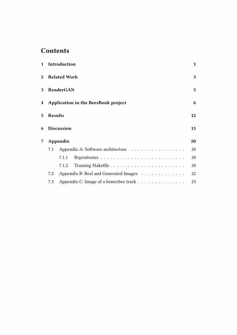
Figure 1: Images generated with the RenderGAN and the corresponding images fromthe 3D model.

One approach to collect labeled data at low costs is to generate them. Often abasic model of the data exists, for example, a 3D model of a human with the basicjoint con�guration. Su et al., 2015b used a computer graphics pipeline to generatea large amount of labeled data. Even though computer graphics can achievestunning visual results, it is hard to select the right parameters to match thestatistics of the real data. For example, to reproduce the same lighting conditionsas in real data, the distribution of position and intensity of the light sources mustbe reconstructed. This can become complex if, for example, the intensity of thelight depends on the object type.The recently introduced Generative Adversarial Network (GAN) framework (Good-

1

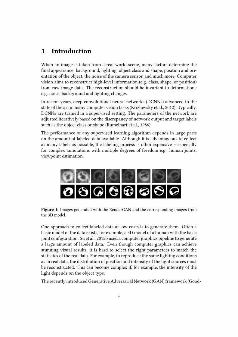
fellow et al., 2014) is capable of generating very realistic images. A generator net-work learns to model the data through an adversarial game. Denton et al., 2015synthesized samples with the GAN framework reproducing the CIFAR dataset(Krizhevsky, 2009) that were hard for humans to distinguish from real images.In my novel RenderGAN framework, I combine a 3D model and a GAN. TheRenderGAN framework renders a 3D model realisticly by learning the missingdeformations (e.g. blurriness, lighting, background, and details) from unlabeleddata. I construct the deformations such that the high-level information of the3D model cannot change. Therefore, I can generate images where the labels areknown from the 3D model and that look strikingly real due to the GAN frame-work.The RenderGAN framework was developed as a solution to a real-world prob-lem in the BeesBook project (Wario et al., 2015). Hence, my experiments areconducted on data from the BeesBook project. The goal of the BeesBook projectis to analyze the social behavior of honeybees. This analysis is performed bytracking all bees individually over multiple weeks. A binary tag is attached tothe bees for identi�cation (see Fig. 2). An existing computer vision pipeline didnot show the performance needed to track the bees reliably. Hence, I wanted toimprove the decoding of the binary tags.The annotation of a tag in an image is time-consuming, as it requires one to set12-bits, two coordinates, and three angles. I automated this task with the Ren-derGAN framework by generating realistic labeled data. Our only supervisionis a basic 3D model (see the lower row of Fig. 1). I train a DCNN on the gener-ated labeled data to decode the bee tag. This neural network performs well whentested on real images of bee tags.To my best knowledge, I do not know of any other work that was able to gener-ate data of su�cient quality to train a DCNN from scratch on it and which stillperformed well on real data.In the next section 2, I provide an overview of the related work and shortly reviewof the GAN framework. In section 3, I introduce image deformation functionsand derive the RenderGAN framework. Section 4 covers the application of theRenderGAN in the BeesBook project. I then describe the performance of a DCNNtrained solely on generated images and tested on real data in section 5. I discussadvantages and limitations of the RenderGAN framework in section 6 and givean outlook for future work.

2

6 43

0109

11 12

58

71312

(a) Tag structure (b) Tagged bees in the hive

Figure 2: (a) The tag represents a unique binary code (cell 0 to 11) and encodes theorientation with the semicircles 12 and 13. The red arrow ↑ visualizes the orientation.It points to the head of the bee. The bit con�guration is read starting at cell 0. Here,100110100010 is shown. (b) Cutout from a high-resolution image

2 Related Work

The related work stems from two directions: Generative adversarial networksand using synthetic images in computer vision.Synthetic images: Stark et al., 2010 used 3D CAD models to build a multi-view object class detector. Dosovitskiy et al., 2014 showed that a DCNN canemulate 3D models of chairs to near perfection. Recently, Su et al., 2015a traineda DCNN to recognize the shapes of 3D CAD data by rendering the 3D model frommultiple viewpoints. Su et al., 2015b utilized synthetic images to achieve stateof the art results on the viewpoint estimation task on the PASCAL 3D+ dataset(Xiang et al., 2014). The PASCAL 3D+ dataset contains around 36000 images of12 categories (e.g. airplanes or cars) annotated with the viewpoint and 3D modelof the object. Although Su et al., 2015b claim their generated data is resistantto over�tting, they do not train a DCNN from scratch on it. Their DCNN isinitialized with weights from Malik et al., 2014, which in turn is trained on datafrom the ImageNet database (Deng et al., 2009). They adapt the network to theviewpoint estimation task by training the last layers with generated data, whilea small real dataset is used to �ne-tuning all layers.

3

real data

noise0-1

G

Dfake

Figure 3: Topology of a Generative Adversarial Network (GAN). The discriminator net-work is trained to distinguish between generated and real data. The generator networkproduces fake images from a random source and is optimized to maximize the chance ofthe discriminator to make a mistake.

Generative Adversarial Networks: In the GAN framework (Goodfellow et al.,2014), a generative model is obtained through optimizing a minimax game. Thegenerative model G is pitted against a discriminator model D . D(x) is optimizedto predict the probability of x being from the real data or generated by G. G, inturn, is trained to maximize the chance of the discriminator to make a mistake.Goodfellow et al., 2014 showed that for arbitrary functionsG andD a unique so-lution to this minimax game exists whereG learns to model the data distributionand D cannot separate between generated and real data.Usually, neural networks are used for G and D . G receives a random vector z asinput and generates sample to "fool" the discriminator. If for example, a GAN istrained on images of human faces, then at the beginning of the training G willjust produce noisy images unrelated to faces. D now learns to spot the generatedimages. G, in turn, improves as it learns that the images containing colors similarto faces are scored more realistic. This forces again D to adapt. The competitiondrives both G and D to improve. G learns to model more sophisticated features,while D tries to pick up new features to distinguish between generated and realdata.The formal objective of the minimax game is:

minG

maxD

Ex∼PData[logD(x)] +Ez∼noise[log(1−D(G(z)))] (1)

The �rst part of the objective represents the performance of the D on the realdata. It is maximal if D can perfectly spot real images. The second part re�ectshow well the discriminator can detect generated data. The generator is trainedto minimize the second expectation by producing images that D scores as real.A simple extension of the GAN framework ist the so-call conditional GAN (cGAN).Both generator and discriminator are conditioned on a variable, e.g. with the ob-ject class of an image. If G generates data not matching the conditional variable,D will use this as a feature to distinguish it from the real data which matches the

4

conditional variable. Even though the training process requires annotations tothe data, once the training converges one can sample data given a label.

3 RenderGAN

real data

noise

0-1

G

D

M φ0 φk. . . fake

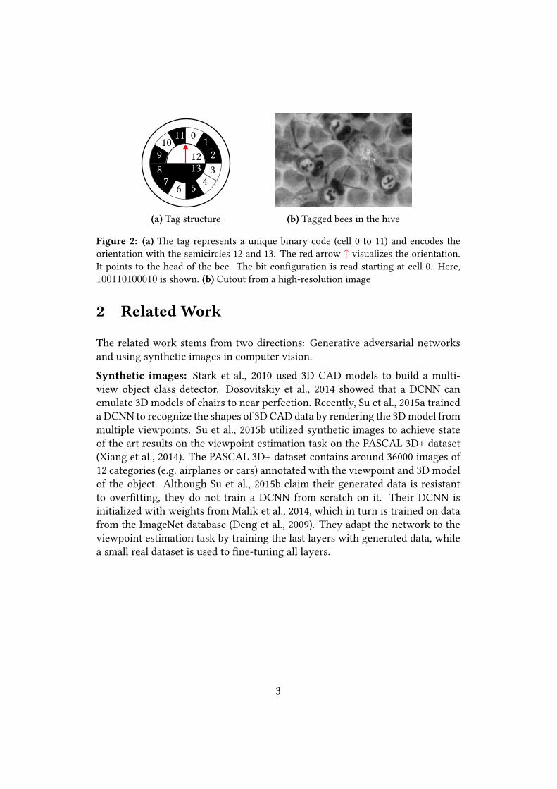
Figure 4: The generator G cannot directly produce fake images. Instead, G has to usea 3D model M to generate a simple image, which is then modi�ed by G through thedeformation functions φ to match the real data.

For this analysis, I consider a regression task: �nd an approximation to a givenfunction f̂ :Rn 7→ L, that maps from data space Rn to label space L. I consider f̂to be the best available function on this particular task. Analog to ground truthdata, I will call f̂ ground truth function. In most cases f̂ is simply a human expert.Using f̂ is expensive. Therefore only a small amount of labeled data exists.Suppose I have a simple 3D model that maps high-level information to an image.It is important that the 3D model captures the coarse structure of the object,but its generated image might lack many factors that are contained in the realimages. For example, the 3D model might lack lighting, background, and details.The goal is to add the missing factors while preserving the labels.I start by modeling an image deformation as a function φ(x,d) on an image xand a deformation d (d can be a tensor of any rank). The image deformationmust preserve the labels of the image x. Therefore it must hold for all images xand all deformation vectors d:

f̂ (φ(x,d)) = f̂ (x) (2)

A second requirement is that the deformation function must be di�erentiablew.r.t. d as the gradient will be back-propagated through φ to the generator.Image deformations like lighting, surrounding, and noise do not change the la-bels and �t this de�nition. I will provide appropriate de�nitions of φ for thementioned deformations in the following chapter.

5

If appropriate φ functions are found that can model the missing image deforma-tions and are di�erentiable, the GAN framework can be used to �nd parametersto the image deformations to make the resulting image realistic. The generatorG provides k di�erent outputs for all k deformations.

g(z) = φ0(φ1(. . .φk(M(Gl(z)),Gk(z)) . . . ,G1(z)),G0(z)) (3)

A visual interpretation of this formula is shown in Figure 4. g(z) correspondsto the generator in the conventional GAN framework. The discriminator lossis backpropagated through the 3D model M and the functions φ to adapt G.Therefore, also M must be di�erentiable. A 3D software model can be made dif-ferentiable by training a DCNN to emulate it. As the label distribution can becomplex, the generator also learns to model it. Alternatively, if the label distri-bution is known, one could sample the labels randomly.Please note, that the theoretical guarantees of the conventional GAN training stillhold. If the training converges, the generator has learned to replicate the datadistribution, while the discriminator can no longer separate between real andgenerated data. However, in a real application, theφ functions might restrict thegenerator from perfectly replicating the data distribution.Once the training converges, I can collect generated realistic data with g(z) andhigh-level information with Gl(z). As the deformation functions are built suchthat the labels do not change, the ground truth function f̂ will recover f̂ (g(z)) =Gl(z). The goal was to approximate the ground truth function f̂ . This can nowbe done by training a supervised learning algorithm on generated data g (z) andthe high-level information Gl (z).

4 Application in the BeesBook project

In the BeesBook project, we aim to understand the complex social behavior ofhoney bees. For the analysis, we rely on the trajectories of honeybees. A binarytag is attached to the torso of the bees. As the orientation, position, and tag id areneeded to build the trajectories, I want to train a neural network to extract themfrom raw image data. The goal is to synthesize images where the id, position,and rotation of the tags are known. And which are realistic enough to train aneural network from scratch on them.The 3D model takes the position, orientation, and id of a tag as input and syn-thesizes images that represent the given tag parameters. However, the generatedimages lack many important factors: lighting, blurriness, background, and de-

6

outputs:

zid

zoffset

3d model φblur φlighting φbg φdetail

G

0.48

Figure 5: Deformation functions of the RenderGAN in the BeesBook project. The inputsto the deformation functions are shown on the arrows from G to the deformation func-tions φ. On top, the output of each stage is shown. The output of φdetail is forwardedto the discriminator as the �nal generated image.

tails (see the lower row in Fig. 1). The background pixels are specially markedby the 3D model. This will be later useful to add the background at the rightlocation. Furthermore, it produces a depth map of the object which showed tobe bene�cial to generate more realistic images.As the distribution of the position and orientation of the tag are unknown, thegenerator also learns to predict them. Whereas the bits of the id are chosen atrandom. The discriminator loss must be backpropagated through the 3D modelto the generator. Therefore, I train a neural network to emulate the 3D model.This network is called 3D network. Its output is undi�erentiable from the imagesof the 3D model. The weights of the 3D network are �xed during the RenderGANtraining.I construct the generator so that it can �ll in the missing factors. I apply di�er-ent deformation functions that account for lighting, blurriness, background anddetails. The output images of all deformation stages are always in the range -1to 1. This is done with the later introduced in bounds layer.Blurriness: The 3D model produces hard edges, but the images of the real tagsshow a wide range of blurriness. The generator produces a scalar ω ∈ [0,1] perimage that controls the amount of blurriness. The implementation of the blurfunction is inspired by Laplacian pyramids (Burt and Adelson, 1983).

b(x) = x ∗ kσ (4)φblur(x,ω) = (1−ω) (x − b (x)) + b(x) (5)

7

0.25 0.09 0.80 0.03

0.35 0.70 0.23 0.40

(a) Generated

0.44 0.21 0.00 1.00

0.00 0.10 0.00 0.18

(b) Real

Figure 6: Discriminator scores for generated and real images.

kσ denotes a Gaussian kernel, with scale σ . The blurred image b(x) is obtained byconvolving the image with the Gaussian kernel kσ . I used σ = 3, which providesenough blurriness and still preserves the labels. As required for deformationfunctions, the function is di�erentiable w.r.t to the inputω and the labels are notchanged.

input:0-1 1

black white

scale:

shift:

clip:0-1 1

Figure 7: Operations of the Lighting deformation. The colored intervals show possiblevalues of black or white pixels. First, the binary input of either -1 or 1 is scaled. Byrestricting the amount of the scaling, it is ensured that the bits do not �ip. In the nextoperation, the pixel intensities are shifted to model all possible lighting conditions. Ashift of 0.5 is visualized in this graphic. The �nal clip operation ensures that the outputis in the range -1 to 1 and is implemented with the in bounds layer.

Lighting of the tag: The images of the 3D model are either black or white.In real images, tags exhibit all di�erent shades of gray. I model the lighting by asmooth scaling and shifting of the pixel intensities. The generator provides threeoutputs for the lighting: scaling of black parts sb, scaling of white parts sw anda shift t. All outputs have the same dimensions as the image x. An importantinvariant is that the black bits of the tag must stay darker than the white bits.Otherwise, a bit could �ip, and the label would change. By restricting the scalingsw and sb to be between 0.10 and 1, I ensure that this invariant holds. The lighting

8

should cause smooth changes in the image. Hence, Gaussian blur b(x) is appliedto sb, sw, and t.

w(x) =

1 if x > 00 if x ≤ 0

(6)

φlighting(x,sw, sb, t) = x ·w(x) · b(sw) + x · (1−w(x)) · b(sb) + b(t) (7)

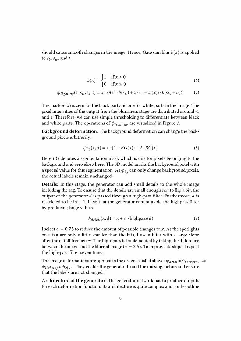
The maskw(x) is zero for the black part and one for white parts in the image. Thepixel intensities of the output from the blurriness stage are distributed around -1and 1. Therefore, we can use simple thresholding to di�erentiate between blackand white parts. The operations of φlighting are visualized in Figure 7.Background deformation: The background deformation can change the back-ground pixels arbitrarily.

φbg(x,d) = x · (1−BG(x)) + d ·BG(x) (8)

Here BG denotes a segmentation mask which is one for pixels belonging to thebackground and zero elsewhere. The 3D model marks the background pixel witha special value for this segmentation. Asφbg can only change background pixels,the actual labels remain unchanged.Details: In this stage, the generator can add small details to the whole imageincluding the tag. To ensure that the details are small enough not to �ip a bit, theoutput of the generator d is passed through a high-pass �lter. Furthermore, d isrestricted to be in [−1,1] so that the generator cannot avoid the highpass �lterby producing huge values.

φdetail(x,d) = x+α · highpass(d) (9)

I select α = 0.75 to reduce the amount of possible changes to x. As the spotlightson a tag are only a little smaller than the bits, I use a �lter with a large slopeafter the cuto� frequency. The high-pass is implemented by taking the di�erencebetween the image and the blurred image (σ = 3.5). To improve its slope, I repeatthe high-pass �lter seven times.The image deformations are applied in the order as listed above: φdetail◦φbackground◦φlighting◦φblur . They enable the generator to add the missing factors and ensurethat the labels are not changed.Architecture of the generator: The generator network has to produce outputsfor each deformation function. Its architecture is quite complex and I only outline

9

the most important parts. My code is available online with all the details of thenetworks 1.The generator starts with a small network consisting of dense layers, that pre-dicts the parameters for the 3D model (position, orientations). As mentionedbefore, the id is sampled uniformly at random.A combination of a dense and reshape layer – Radford et al., 2015 call this pro-jection layer – is used to start a chain of convolutional and upsampling layers. Inthe generator network, a common build block is a 3x3 convolutional layer, batchnormalization (Io�e and Szegedy, 2015), ReLU activation (Nair and Hinton, 2010)and upsampling.I found it advantageous to merge a depth map of the 3D model into the generatoras especially the lighting depends on the orientation of the tag in space. An extranetwork is branched o� to predict the input for the lighting deformation. Theinput to the blur deformation is predicted by reducing an intermediate represen-tation with a convolutional layer with a single output feature map and a denselayer to a single scalar.For the background generation, the output of the lighting network is mergedback into the main generator network. The generator network can utilize theimage produced by the 3D network to learn the input to the detail deformation.

−3 −2 −1 0 1 2 3

Input

−1.0−0.50.0

0.5

1.0

1.5

Loss

/Out

put

a bLossActivation

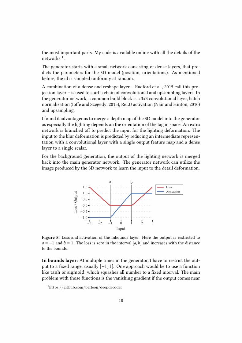
Figure 8: Loss and activation of the inbounds layer. Here the output is restricted toa = −1 and b = 1. The loss is zero in the interval [a,b] and increases with the distanceto the bounds.

In bounds layer: At multiple times in the generator, I have to restrict the out-put to a �xed range, usually [−1;1]. One approach would be to use a functionlike tanh or sigmoid, which squashes all number to a �xed interval. The mainproblem with those functions is the vanishing gradient if the output comes near

1https://github.com/berleon/deepdecoder

10

the bounds of the interval.I am using a combination of clipping and activity regularization to keep the out-put in a given interval [a,b]. I call this combination in bounds layer as it keeps theoutput in bounds. If the input x is out of bounds, it is clipped to be in bounds anda regularization loss l depending on the distance between x and the appropriatebound is added (see Fig. 8).

l(x) =

w||x − a||1 if x < a0 if a ≤ x ≤ bw||x − b||1 if x > b

(10) f (x) = min(max(a,x),b) (11)

With the scalar w, the weight of the loss can be adapted. If the in bounds layersin the generator are replaced with tanh activations, the GAN training does notconverge.

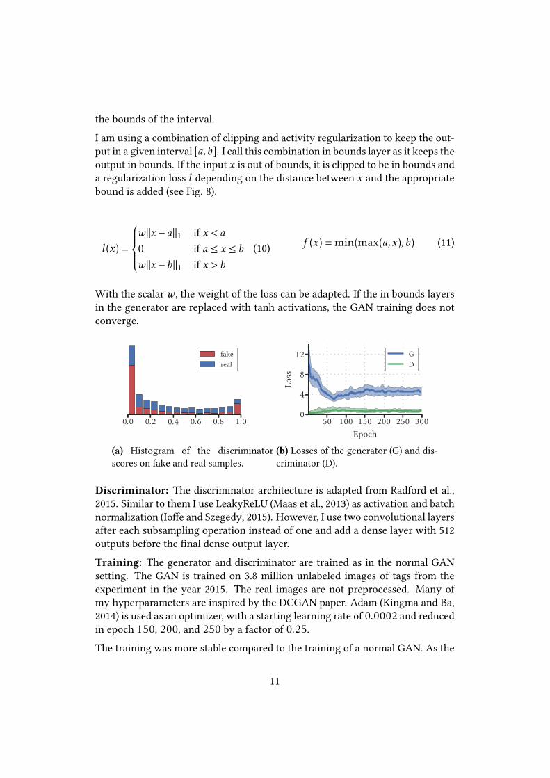
0.0 0.2 0.4 0.6 0.8 1.0

fakereal

(a) Histogram of the discriminatorscores on fake and real samples.

50 100 150 200 250 300

Epoch

0

4

8

12

Loss

GD

(b) Losses of the generator (G) and dis-criminator (D).

Discriminator: The discriminator architecture is adapted from Radford et al.,2015. Similar to them I use LeakyReLU (Maas et al., 2013) as activation and batchnormalization (Io�e and Szegedy, 2015). However, I use two convolutional layersafter each subsampling operation instead of one and add a dense layer with 512outputs before the �nal dense output layer.Training: The generator and discriminator are trained as in the normal GANsetting. The GAN is trained on 3.8 million unlabeled images of tags from theexperiment in the year 2015. The real images are not preprocessed. Many ofmy hyperparameters are inspired by the DCGAN paper. Adam (Kingma and Ba,2014) is used as an optimizer, with a starting learning rate of 0.0002 and reducedin epoch 150, 200, and 250 by a factor of 0.25.The training was more stable compared to the training of a normal GAN. As the

11

coarse structure of the tags is already learned by the 3D network, the generatorcannot collapse to one sample as sometimes seen in GAN training.In few samples, the generator destroys the image by adding many high frequen-cies. I did not do any deeper investigations why this occurs. As those bad sam-ples are scored unrealistic by the discriminator without exception, they can beremoved for the training of the supervised algorithm.The generator does not converge to the point where D cannot di�erentiate be-tween real and fake (see Fig. 9a). This is due to some samples (mostly very blurry)that cannot be created by G with the given deformation functions. Another ob-stacle might be that the ids are uniformly sampled, but not uniformly distributedin the training set. Some bees have died early or lost their tag. If the discrimina-tor learns this feature, the generator can augment the 3D model perfectly, but thediscriminator will still spot them. However, I did not evaluate if this hypothesisis indeed true.In the end, I am not interested in the relative relationship of the GAN losses toeach other, but if the generated samples are realistic enough to train a neuralnetwork on them. The training set is build from the generated images and thecorresponding labels at the input to the 3D network. In the next section, I showthe results of a DCNN solely trained on this generated training set.

5 Results

I describe the DCNN trained with the synthetic data to decode bee tags, the originof the test set and compare the DCNN to the previously used computer visionpipeline. The comparison includes the accuracy, con�dence, and speed.The architecture of the decoder network (see Fig. 10) is based on the ResNetarchitecture recently introduced by He et al., 2015. By using skip connections,deeper neural networks can be trained with the ResNet architecture. The net-work is trained with standard stochastic gradient descent with momentum.For training, I am using a synthetic training set generated with the RenderGANframework. The test set is extracted from ground truth data that was originallycollected to evaluate bee trajectories. This data contains the path and id of eachbee over multiple consecutive frames. In total, I collect 50k real images of tagslabeled with the tag id.Unfortunately, the position of the tags varies more in the test data then in thetraining data for the GAN, due to human errors and bad generated proposals.The test set also stems from experiments in years 2014 and 2015. Whereas, the

12

layer name output size layerinput 64x64 -conv1 32x32 3x3, 16, stride 2

conv2_x 32x32[3x3, 163x3, 16

]× 3

conv3_x 16x16[3x3, 323x3, 32

]× 4

conv4_x 8x8[3x3, 643x3, 64

]× 6

conv5_x 4x4[3x3, 1283x3, 128

]× 3

id 12 fc 256, fc 12params 6 fc 256, fc 6

Figure 10: Architecture of the decoder network. The brackets denote ResNet buildingblocks. The id and params layer receive both the output from layer conv5_3 as input.The output of the params layer represents the orientation, position, and radius. As inthe original ResNet architecture, downsampling is performed by conv3_1,conv4_1, andconv5_1 with a stride of 2.

RenderGAN was only trained on data from 2015. Furthermore, the data from2014 is more blurry and has less contrast. I employ aggressive data augmentation(e.g. shearing, small rotation, and additional noise) and preprocess the imageswith a histogram equalization so that the decoder network can generalize to thedi�erent data from the year 2014.Before the RenderGAN framework, a computer vision pipeline based on manualfeature extraction was used to decode the tags. The computer vision pipelineconsists of multiple stages: preprocessor, localizer, ellipse �tter, grid �tter anddecoder. The preprocessor applies image transformations like CLAHE to theinput. In the localizer stage, honey bees are found with an edge detector andmorphological operations. A neuronal network sorts out false detections of thelocalizer. A modi�ed Hough transformation �nds ellipses in the edge images.The grid �tter uses gradient descent to match a 3D model of the tag onto theimage. The decoder stage �nally reads the bit values from the tag.One metric to evaluate how well the ids of the tags are decoded is the meanHamming distance (MHD) which is the expectation of the number of wrong bitsper detection. The decoder network is more accurate with a mean Hamming dis-tance of 0.17 compared to 1.08 of the computer vision pipeline. In the evaluationof the computer vision pipeline, occluded bits are not counted, whereas they arenot marked in the test set for the decoder network.The decoder network provides continuous outputs, which can be interpreted as

13

20 40 60 80 100

Epoch

0.0

0.2

0.4

0.6

0.8

Loss

trainval

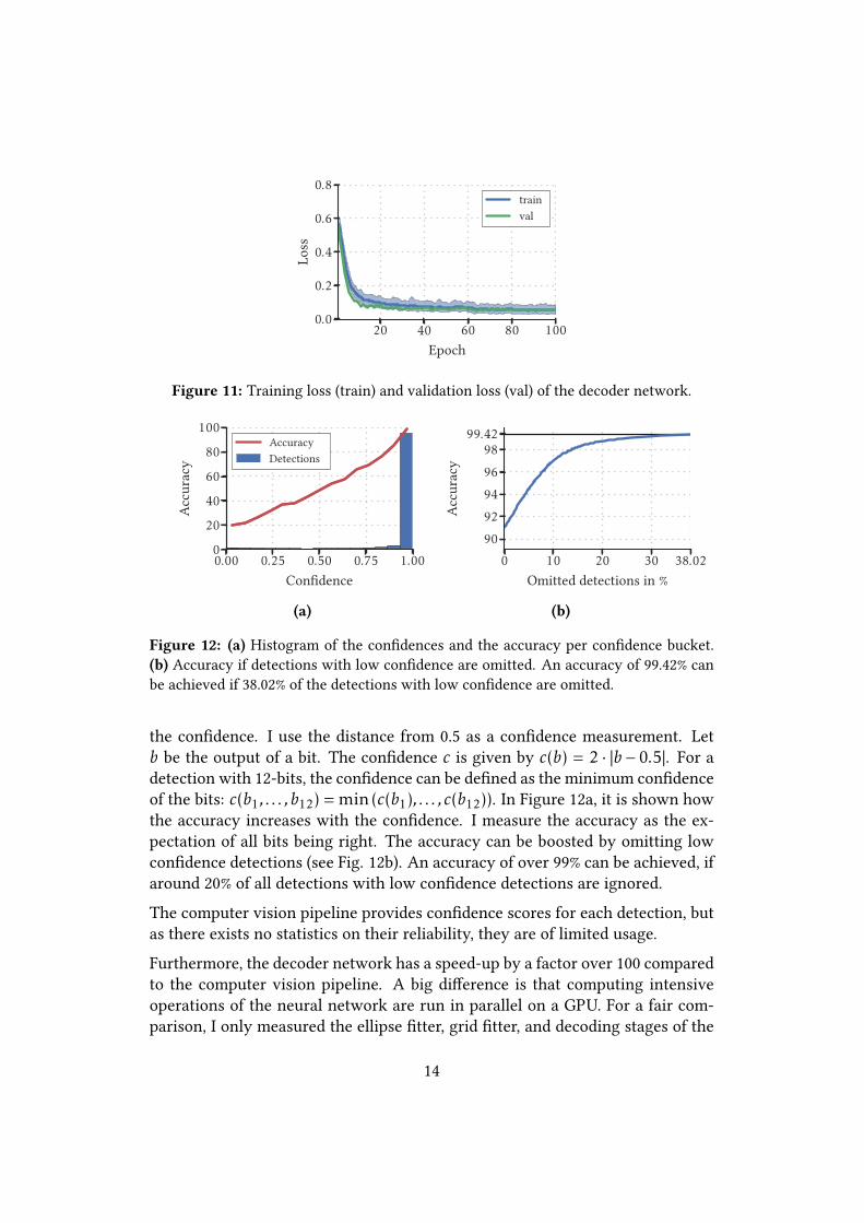
Figure 11: Training loss (train) and validation loss (val) of the decoder network.

0.00 0.25 0.50 0.75 1.00

Con�dence

0

20

40

60

80

100

Accu

racy

AccuracyDetections

(a)

0 10 20 30 38.02

Omitted detections in %

90

92

94

96

9899.42

Accu

racy

(b)

Figure 12: (a) Histogram of the con�dences and the accuracy per con�dence bucket.(b) Accuracy if detections with low con�dence are omitted. An accuracy of 99.42% canbe achieved if 38.02% of the detections with low con�dence are omitted.

the con�dence. I use the distance from 0.5 as a con�dence measurement. Letb be the output of a bit. The con�dence c is given by c(b) = 2 · |b − 0.5|. For adetection with 12-bits, the con�dence can be de�ned as the minimum con�denceof the bits: c(b1, . . . , b12) = min(c(b1), . . . , c(b12)). In Figure 12a, it is shown howthe accuracy increases with the con�dence. I measure the accuracy as the ex-pectation of all bits being right. The accuracy can be boosted by omitting lowcon�dence detections (see Fig. 12b). An accuracy of over 99% can be achieved, ifaround 20% of all detections with low con�dence detections are ignored.The computer vision pipeline provides con�dence scores for each detection, butas there exists no statistics on their reliability, they are of limited usage.Furthermore, the decoder network has a speed-up by a factor over 100 comparedto the computer vision pipeline. A big di�erence is that computing intensiveoperations of the neural network are run in parallel on a GPU. For a fair com-parison, I only measured the ellipse �tter, grid �tter, and decoding stages of the

14

CV pipeline Decoder networkMean Hamming Dist. 1.08 0.17

Time per Tag [ms] 177.54 1.43Tracking: Id Accuracy 55% 96%

Con�dence limited usage yesGeneralization No, �ne-tuned per camera

and recording setttinggeneral

Language C++ Python

Figure 13: Tabular comparison of the computer vision pipeline and the decoder net-work.

computer vision pipeline. The computer vision pipeline is benchmarked on �veimages and the decoder network on the whole test set.The evaluation and benchmark of the computer vision pipeline could be donemore rigorous, but given the large di�erence in speed and accuracy, this wouldhardly change the overall picture.Another advantage of the decoder network is its generalization power. Theweights of the network work across di�erent recording settings. In contrast, thehyperparameters of computer vision pipeline must be �ne-tuned for any changesin the recording settings and for every camera.First tests on the tracking of honeybees also underline the better performanceof the decoder network. Tracking done with detections of the computer visionpipeline resulted in 55% of all ids being assigned correctly. With data from thedecoder network, this number increased to 96% (see Fig. 15 in the appendix foran exemplary track).

6 Discussion

The proposed RenderGAN framework was shown to render a 3D model realisticso that a DCNN could be trained with the generated data and performed well onreal data.Complex deformations (e.g. background, lighting, and details) were learned fromunlabeled data. The GAN training procedure ensured that the generated imagesmatch the statistics of the real data. This task is di�cult to solve with a conven-tional computer graphics pipeline as it is di�cult to model implicit connectionsin the data. For example, even if the 3D model of the tag were extended to includelighting, the distribution of intensity and position of the light source would be

15

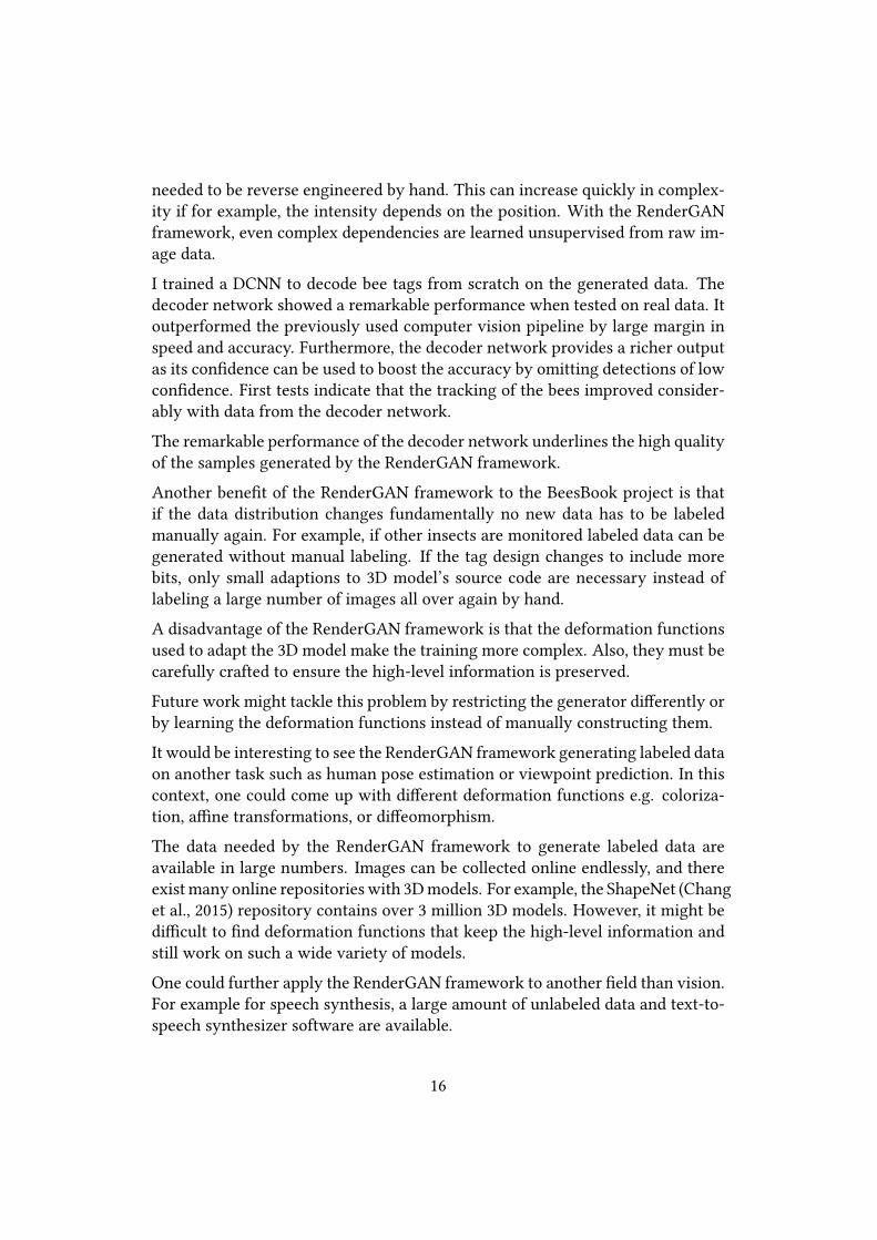
needed to be reverse engineered by hand. This can increase quickly in complex-ity if for example, the intensity depends on the position. With the RenderGANframework, even complex dependencies are learned unsupervised from raw im-age data.I trained a DCNN to decode bee tags from scratch on the generated data. Thedecoder network showed a remarkable performance when tested on real data. Itoutperformed the previously used computer vision pipeline by large margin inspeed and accuracy. Furthermore, the decoder network provides a richer outputas its con�dence can be used to boost the accuracy by omitting detections of lowcon�dence. First tests indicate that the tracking of the bees improved consider-ably with data from the decoder network.The remarkable performance of the decoder network underlines the high qualityof the samples generated by the RenderGAN framework.Another bene�t of the RenderGAN framework to the BeesBook project is thatif the data distribution changes fundamentally no new data has to be labeledmanually again. For example, if other insects are monitored labeled data can begenerated without manual labeling. If the tag design changes to include morebits, only small adaptions to 3D model’s source code are necessary instead oflabeling a large number of images all over again by hand.A disadvantage of the RenderGAN framework is that the deformation functionsused to adapt the 3D model make the training more complex. Also, they must becarefully crafted to ensure the high-level information is preserved.Future work might tackle this problem by restricting the generator di�erently orby learning the deformation functions instead of manually constructing them.It would be interesting to see the RenderGAN framework generating labeled dataon another task such as human pose estimation or viewpoint prediction. In thiscontext, one could come up with di�erent deformation functions e.g. coloriza-tion, a�ne transformations, or di�eomorphism.The data needed by the RenderGAN framework to generate labeled data areavailable in large numbers. Images can be collected online endlessly, and thereexist many online repositories with 3D models. For example, the ShapeNet (Changet al., 2015) repository contains over 3 million 3D models. However, it might bedi�cult to �nd deformation functions that keep the high-level information andstill work on such a wide variety of models.One could further apply the RenderGAN framework to another �eld than vision.For example for speech synthesis, a large amount of unlabeled data and text-to-speech synthesizer software are available.

16

References

[1] Peter Burt and Edward Adelson. “The Laplacian pyramid as a compactimage code”. In: IEEE Trans. Commun. 9.4 (1983), pp. 532–540.

[2] Angel X. Chang et al. ShapeNet: An Information-Rich 3D Model Repository.2015. arXiv: 1512.03012.

[3] Jia Deng et al. “ImageNet: A large-scale hierarchical image database”. In:2009 IEEE Conference on Computer Vision and Pattern Recognition (2009).issn: 1063-6919. doi: 10.1109/CVPR.2009.5206848.

[4] Emily Denton et al. Deep Generative Image Models using a Laplacian Pyra-mid of Adversarial Networks. 2015. arXiv: 1506.05751.

[5] Alexey Dosovitskiy, Jost Tobias Springenberg, and Thomas Brox. “Learn-ing to Generate Chairs with Convolutional Neural Networks”. In: IEEECVPR (2014). issn: 1098-6596. doi: 10.1109/CVPR.2015.7298761. arXiv:1411.5928.

[6] Ian Goodfellow et al. “Generative Adversarial Nets”. In: Advances in Neu-ral Information Processing Systems 27. Ed. by Z. Ghahramani et al. CurranAssociates, Inc., 2014, pp. 2672–2680.

[7] Kaiming He et al.Deep Residual Learning for Image Recognition. 2015. arXiv:1512.03385.

[8] Sergey Io�e and Christian Szegedy. BatchNormalization: AcceleratingDeepNetwork Training by Reducing Internal Covariate Shift. 2015. arXiv: 1502.03167.

[9] Diederik Kingma and Jimmy Ba. Adam: A Method for Stochastic Optimiza-tion. 2014. arXiv: 1412.6980.

[10] Alex Krizhevsky. Learning Multiple Layers of Features from Tiny Images.2009. doi: 10.1.1.222.9220. arXiv: arXiv:1011.1669v3.

[11] Alex Krizhevsky, Ilya Sutskever, and Geo�rey E. Hinton. “ImageNet Clas-si�cation with Deep Convolutional Neural Networks”. In:Advances in Neu-ral Information Processing Systems 25. Ed. by F. Pereira et al. Curran Asso-ciates, Inc., 2012, pp. 1097–1105.

[12] Andrew L. Maas, Awni Y. Hannun, and Andrew Y. Ng. “Recti�er nonlin-earities improve neural network acoustic models”. In: ICML Workshop onDeep Learning for Audio, Speech and Language Processing 28 (2013).

17

[13] Jitendra Malik et al. “Rich Feature Hierarchies for Accurate Object Detec-tion and Semantic Segmentation”. In: 2014 IEEE Conference on ComputerVision and Pattern Recognition (CVPR) (2014), pp. 580–587. issn: 10636919.doi: 10.1109/CVPR.2014.81. arXiv: 1311.2524.

[14] Vinod Nair and Geo�rey E Hinton. “Recti�ed Linear Units Improve Re-stricted Boltzmann Machines”. In: Proceedings of the 27th International Con-ference on Machine Learning 3 (2010), pp. 807–814. issn: 1935-8237. doi:10.1.1.165.6419.

[15] Alec Radford, Luke Metz, and Soumith Chintala. Unsupervised Represen-tation Learning with Deep Convolutional Generative Adversarial Networks.2015. arXiv: 1511.06434.

[16] D E Rumelhart, G E Hintont, and R J Williams. “Learning representationsby back-propagating errors”. In: Nature 323.6088 (1986), pp. 533–536. issn:0028-0836. doi: 10.1038/323533a0.

[17] Michael Stark, Michael Goesele, and Bernt Schiele. “Back to the Future:Learning Shape Models from 3D CAD Data.” In: BMVC (2010). doi: 10 .5244/C.24.106.

[18] Hang Su et al. “Multi-view Convolutional Neural Networks for 3D ShapeRecognition”. In: The IEEE International Conference on Computer Vision(ICCV). 2015. isbn: 978-1-4673-8391-2. doi: 10 . 1109 / ICCV . 2015 . 114.arXiv: 1505.00880.

[19] Hao Su et al. “Render for CNN: Viewpoint Estimation in Images UsingCNNs Trained with Rendered 3D Model Views”. In: The IEEE InternationalConference on Computer Vision (ICCV). 2. 2015. isbn: 978-1-4673-8391-2.doi: 10.1109/ICCV.2015.308. arXiv: 1505.5641.

[20] Fernando Wario et al. “Automatic methods for long-term tracking and thedetection and decoding of communication dances in honeybees”. In: Fron-tiers in Ecology and Evolution 3.September (2015). issn: 2296-701X. doi:10.3389/fevo.2015.00103.

[21] Yu Xiang, Roozbeh Mottaghi, and Silvio Savarese. “Beyond PASCAL: Abenchmark for 3D object detection in the wild”. In: 2014 IEEE Winter Con-ference onApplications of Computer Vision,WACV 2014. 2014. isbn: 9781479949854.doi: 10.1109/WACV.2014.6836101.

18

7 Appendix

7.1 Appendix A: Software architecture

7.1.1 Repositories

Through the thesis multiple repositories were created.diktya: contains a implementation of the GAN framework, general utilities totrain neural networks, helper functions for plotting, and extensions to the keraslibrary. Its content is general enough to be used by other parties.beesgrid: provides a boost python wrapper to the C++ 3D model. It is usedto generated the training data to emulate the 3D object model with a neuronalnetwork.bb_binary: a binary format based on Cap’n Proto to store the detections of thedecoder network. Before a CSV format was used. The binary format reduces the�le size by a factor of 4 and can more importantly hold detections to more thanone image or video.deepdecoder: contains the code to train the di�erent neuronal networks andto create the arti�cial training set. A Make�le is provided to automate the dataacquisition and training process.

7.1.2 Training Make�le

There are only three inputs needed to train a decoder network: a trained localizernetwork, a large number of high-resolution images of the hive, and ground truthdata. The localizer network �nds the position of the tagged honeybees in thehigh-resolution images. And the ground truth data is needed to evaluate thetrained decoder. Still, there exist mutliple programs that must be executed:

• bb_�nd_tags: �nding the bees position in the real images with the local-izer

• bb_preprocess: preprocessing of the real images

• bb_build_tag_dataset: building the real dataset

• bb_generate_3d_tags: sampling a dataset from the 3D model

• bb_train_tag3d_network: training the 3D object network

19

• bb_train_rendergan: running the RenderGAN training procedure

• bb_sample_arti�cial_trainset: sampling an arti�cial training set fromthe generator

• bb_train_decoder: train the decoder on the arti�cial training set and eval-uate the decoder on real ground truth data

Running each program requires domain knowledge. Each program has its ownparameters, requires di�erent inputs, and might depend on other programs to beexecuted before.On the one hand, it is desirable to automate the whole process. This considerablyreduces the cost of training a decoder. On the other hand, training neural net-works always comes with tweaking hyperparameters and network architecture.So the settings of every program must be easily alterable by the user.A good compromise between this two requirements is a Make�le. Each programhas its own build target. One can either run the targets manually and tweak somesettings. Or run ‘make train_decoder‘ to execute all targets and to produce aready to use decoder model. The default settings are selected to maximize theprediction performance of the decoder.For a detailed documentation on the Make�le and training process, please referto the online documentation. 2

2https://github.com/berleon/deepdecoder

20

7.2 Appendix B: Real and Generated Images

(a) Generated images

(b) Real images

Figure 14: Continuum visualization on the basis of the discriminator score: Most realistcscored samples (top) to least realistc (bottom). (a) Samples with image artifacts are scoredunrealistic. (b) Blurry underexposed samples are scored very real as the deformationfunctions restricts the generator to model them.

21

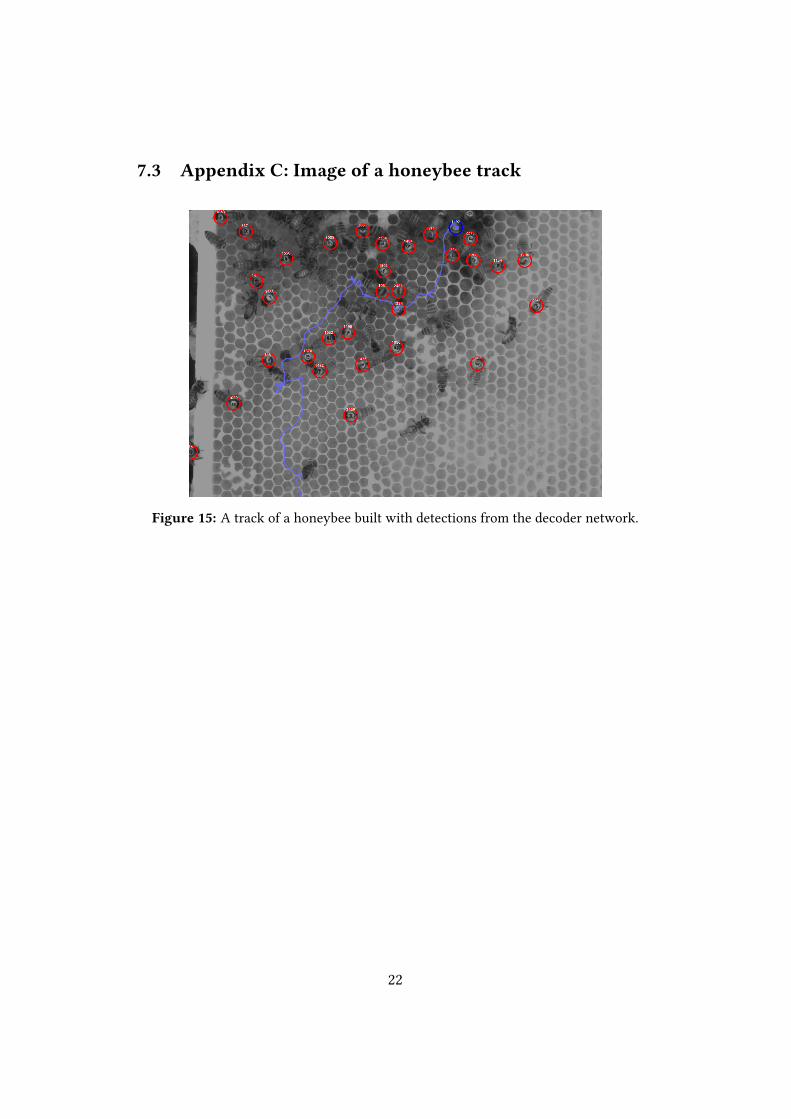
7.3 Appendix C: Image of a honeybee track

Figure 15: A track of a honeybee built with detections from the decoder network.

22