renewable and nonrenewable resource theory applied to

Marine Resource Economics, Volume 9, pp. 291-310 0738-1360/94 $3.00 + .00Printed in the USA. All rights reserved. Copyright © 1994 Marine Resources Foundation

Renewable and Nonrenewable Resource TheoryApplied to Coastal Agriculture, Forest, Wetland,

and Fishery LinkagesSTEPHEN K. SWALLOWDepartment of Resource Economics,University of Rhode Island,Kingston, RI 02881

Abstract This paper addresses tradeoffs in wetland development using aframework that integrates economic theory of renewable and nonrenewableresources. The theory treats wetland development as use of a nonrenewableresource, while wetland preservation protects critical fishery habitat. Theframework recognizes that wetland quality may vary for either development orfisheries. An illustrative application assesses tradeoffs in converting pocosinwetlands to agriculture rather than maintaining wetlands to protect salinity inestuarine nursery areas. Results reveal the marginal value of salinity protec-tion may be substantial, while location may affect a wetland's value to anestuarine shrimp fishery. Comparisons between agricultural and forestry land-uses show that ecological links may cause wetland values to depend upon theland-use chosen for the developed state. Future assessments of other devel-opment may reveal additional impacts through impacts on salinity.

Keywords nonrenewable, renewable, fishery, wetland value, pocosin, Pam-lico Sound

Economic development, such as drainage of coastal wetlands, may impose exter-nal losses on renewable resource production, such as commercial or recreationalfisheries. Several studies address the opportunity costs of preservation (e.g..Brown 1976, Batie and Mabbs-Zeno 1985, Danielson and Leitch 1986, Shabmanand Bertelson 1979) and several others address the external costs of development{e.g., Batie and Wilson 1978; Farber 1987; Kahn and Kemp 1985; Lynne et al.1981). Relatively few studies address both preservation and development, perhapsdue to the natural division between proponents of each or perhaps due to thedifficulty of simultaneously estimating benefits for both. For example, althoughStavins (1990) provides a partial exception, most studies (e.g., Gupta and Foster1975) emphasize the taxonomy of costs and benefits rather than ecological inter-Robert F. Conrad, Diane P. Dupont, James E. Easley, Jr., William F. Hyde, Thomas A.Grigalunas, David H. Newman, Peter J. Parks, Mark G. Smith, James R. Waters, and thereferees motivated improvements to the paper. The National Wildlife Federation; the tJ.S.National Oceanic and Atmospheric Administration grant #NA86AA-D-CZ015; the DuketJniversity Research Council through Duke's School of the Environment; and the RhodeIsland Agricultural Experiment Station (RI AES) funded this research. North Carolinastatistical data were provided at the author's request by the N.C. Division of MarineFisheries (DMF). Analyses of these data and conclusions drawn therefrom are those oftheauthor and do not necessarily represent the views of the N.C. DMF or any fmaneialsponsor. RI AES contribution no. 3024.

297

CORE Metadata, citation and similar papers at core.ac.uk

Provided by Research Papers in Economics

https://core.ac.uk/display/7130509?utm_source=pdf&utm_medium=banner&utm_campaign=pdf-decoration-v1

292 Swallow

dependencies implicit in the wetland allocation issue {cf. Crocker and Tschirhart1992).

This paper addresses tradeoffs implicit in wetland development using a frame-work suggested by integrating the basic theories of renewable and nonrenewableresource economics (Hotelling 1931; Clark and Munro 1975; Swallow 1990). Themodel is tailored to assess issues raised by the historical controversy surroundingthe drainage of coastal wetlands for agriculture on the Pamlico-Albemarle Penin-sula of North Carolina (Heath 1975, NRCD 1987, Street and McClees 1981).Ecologists and fishermen believe that these freshwater wetlands, known as po-cosin wetlands, may be critical to sustaining commercial fisheries in the PamlicoSound estuary, particularly the Penaeid shrimp fishery (Street and McClees 1981).This debate arises, in part, because human-induced ecosystem responses maylimit economic activity and sustainability (see Crocker and Tschirhart 1992) in thePamlico fisheries.

Three objectives motivate this paper: 1) to develop a resource-theoretic ap-proach to marginal preservation-development choices; 2) to apply this frameworkin an assessment of the public issues raised by historical concern regarding po-cosin development; 3) to suggest that cognizance of resource interdependenciescan clarify policy debates. After providing background on the study area, thepaper addresses these objectives in order.

The application relies heavily on the Penaeid shrimp fishery of Pamlico Soundbecause both biological and economic data are available and because ecological or"natural history" theories are sufficient to suggest a plausible approach to assessbiophysical relationships. Furthermore, public concerns often focus on the shrimpfishery because it is by far the largest of Pamlico's fisheries. The assessment-levelapplication offers substantial applied insights as well as illustration, includingempirical results showing that wetland values may depend on the alternativeland-use under consideration. Such key results are revealed by intermediate stepstaken in the empirical assessment of the pocosin development issue.

Study Area: Background and Context

This paper applies a model of interdependent renewable and nonrenewable re-sources to coastal zone development and the Pamlico Sound, NC, Penaeid shrimpfishery. The background for this application will motivate the theoretical structurefor the empirical analysis in subsequent sections.

In the U.S., coastal zone development causes up to 90% of losses in estuarineacreage and indirectly diminishes estuarine productivity through off-site impacts(Tiner 1984). The Pamlico-Albemarle Estuarine Complex is one ofthe largest andmost productive estuarine systems in North America (Epperly and Ross 1986,NRCD 1987). Throughout the U.S., estuarine-dependent fish species comprise50-90% of commercial landings, with North Carolina landings nearly 90% estua-rine-dependent (Epperly and Ross 1986, Street and McClees 1981, Tiner 1984). InPamlico Sound, Penaeid shrimp support the most prized fishery, producing about25% of gross dock-side revenues (Purvis and McCoy 1974, Street and McClees1981). Regionally, however. North Carolina produces a small share {2-4%) ofU.S. landings and ex-vessel prices follow the larger Gulf of Mexico or U.S.markets (Waters et al. 1980).

Recent public debates concern the conflicts between coastal development and

Resource Economic Theory, Wetlands and Fisheries 293

estuarine-dependent vocations (see NRCD 1987). On the preservation side, dis-cussions focus on commercial marine fisheries, especially the highly-valuedshrimp fishery (Street and McClees 1981). On the development side, forestry andagriculture dominate the converted freshwater pocosins (peat-bog wetlands) nearthe estuary (Heath 1975). However, substantial site preparation costs make for-estry and agricultural uses profitable marginally, but these uses remain the dom-inate threat to pocosin wetlands (Heimlich and Langner 1986). No consensusexists concerning what future developers will propose, but predictions range fromurbanization to hog and poultry production to peat mining for electricity genera-tion, with public officials anxious to diversify the area's impoverished economy(Richardson 1981, Tiner 1984, NRCD 1987). Agriculture still motivates policyanalyses {i.e., Palmquist and Danielson 1989) and therefore appears to provide thehighest return.

In this case study, coastal development requires up to 20 miles of drainagecanals per square mile (Heath 1975). Drainage of pocosin wetlands irreversiblyalters the local hydrologic system by eliminating the vegetative and peat-bogstructure that inhibits water flow, causing a decline in the salinity level of estua-rine nursery areas (Heath 1975, Skaggs et al. 1980, Jones and Sholar 1981, Ep-perly and Ross 1986). Rehabilitation of the hydrologic function is viewed as im-practical since the peat-bog structure may take millennia to regenerate.' Thus,wetland development may be assumed irreversible, which is broadly consistentwith the ecology of pocosin wetlands and the engineering of their drainage (Heath1975, NRCD 1987). Irreversibility places wetland development as a nonrenewableresource sector (Krutilla 1967; Fisher and Krutilla 1974).

On the fishery side, Pamlico's juvenile shrimp stock annually arrives via on-shore currents; these currents carry juveniles from an open ocean breedingground to estuarine nurseries along the South Atlantic and Gulf coasts (Epperlyand Ross 1986, Williams 1955). Furthermore, if shrimp escape from the PamlicoSound fishery,^ they generally will not be harvested elsewhere (Williams 1955,McCoy 1972, Purvis and McCoy 1974, Hettler and Chester 1982, Babcock andMundy 1985, Matylewich and Mundy 1985). Finally, an altered hydrologic systemcauses the salinity level to decline in estuarine nurseries, thereby diminishing thesurvival rate of juvenile shrimp (Jones and Sholar 1981, Street and McClees 1981;Williams 1955). Thus, while a fishery is generally viewed as a renewable resourcesector, Pamlico's annual shrimp crop fits the independent-generations fisherymodel (Wilen 1985). This fishery depends upon environmental factors rather thanon a breeding stock.

Economists recognize this process in other fisheries by linking shrimp pro-duction to environmental variables (Blomo et al. 1982, Griffin et al. 1976), buttheir analyses have not linked estuarine environmental variables directly to de-velopment. Irreversible hydrologic impacts suggest wetland development is a typeof nonrenewable resource extraction, the key analogy here.

' Native Americans used "pocosin" to indicate that these wetlands are perched atop a hill;damming of drainage canals is not expected to completely simulate the sponge-like storagecapacity of the original peat soils. Heath (1975) focused on agriculture, while Campbell andHughes (1991) note that modern forestry practices may still preserve hydrologic functions.^ Including Pamlico Sound proper and the Pamlico and Neuse Rivers (U.S. National Ma-rine Fisheries Service areas 6354, 6355, and 7011).

294 Swallow

Theory

The theoretical foundation for this analysis derives from well-known theories ofexploitation for renewable and nonrenewable resources (Hotelling 1931; Clarkand Munro 1975), particularly when these resource sectors are interdependent,such as when the nonrenewable resource provides wetland habitat for the renew-able resource (Swallow 1990). With independent generations in the fishery, theshrimp population X is modeled to depend only upon the habitat stocks E:

X, = X(E»(t),EN(t)), (1)

where E" and E" quantify stocks of "high quality" habitat and "normal quality"habitat, respectively; development determines the habitat available at time t. Inthe renewable sector, fishermen maximize returns or profits R from their labor Land the stock of shrimp, so that renewable resource benefits are:

Rt = R(L*,X(E",E^)) = R*(X), (2)

where L* is the benefit-maximizing quantity of labor conditional on X, so R*represents fishery benefits conditional on the shrimp stock X in a given year. Inthe wetland development sector, nonrenewable resource benefits B' (i = H,N)depend upon the development rate d' and the available stock of wetlands of aparticular type:

B'(d',E') = C(E') d', i = H,N, (3)

where C'(*) denotes the net marginal benefit of an additional acre of developmentfor wetland type i, which depends on the acres remaining, E'. E' indexes thequality of remaining acres from the perspective of development.

Development of pocosin wetlands requires permits through environmentalmanagers, state officials and the U.S. Corps of Engineers under Section 404 oftheU.S. Clean Water Act. Economically, environmental managers must consider thebalance between the present value of wetlands preserved for fisheries and thereturn to wetlands development, at the margin. Then, the economic choice de-pends on the net opportunity cost (NOC) of wetland development:^

NOC'(X,E",E'^) = OR*/aX) • (aX/SE') - r • C'(E') (4)

where NOC is the net opportunity cost of developing wetlands of type i (i =H,N). NOC measures the loss of fishery profits if a marginal unit of E' is devel-oped, net of the annualized return to development. If NOC is positive, denial ofdevelopment permits maximizes social returns from wetlands; if NOC is nega-tive, then approval of development permits returns marginal development benefitsthat more than offset losses in the renewable sector. Since wetland quality may beheterogeneous for either preservation or development, NOC may differ for dif-ferent wetland qualities. The next sections assess the potential for managers to

^ This marginal condition assumes appropriate concavity of (l)-(3).


find NOC is negative, favoring development, for pocosin wetlands near PamlicoSound.

Application

The empirical analysis assumes the Pamlico Sound shrimp fishery: 1) is econom-ically and ecologically independent of neighboring shrimp populations; 2) is af-fected by development; 3) and is a price taker. The link between fishery benefitsand coastal development is generated in a stepwise process which 1) estimates thepotential fishing rents for a given stock of shrimp, 2) links the shrimp stock toestuarine salinity, and 3) links estuarine salinity to development (Fig. 1). Loomis(1988) used a stepwise model in a forestry-fishery context. Our stepwise approachcombines two approaches suggested by Kahn (1987), by including environmentalvariables in the harvest function while also using an (simple) ecosystem model.This approach permits improvements at any step as new scientific or policy in-formation warrants.

Figure 1 illustrates the basic empirical model. Development initiates changesin potential fishery benefits: drainage of pocosin wetlands alters estuarine salinitywhich then lowers the expected annual, estuarine production of shrimp; lowerestuarine productivity alters the conditions of profit maximization; finally, theshrimp fishery realizes a change in expected annual rents. Figure 1 summarizesthe consensus (see above or NRDC 1987) among managers in the Pamlico region.

This consensus (Figure 1) implies three basic relationships:

Marginal Developmentof Pocosin Wetlands

Marginal Return toDevelopment

Salinity Decline

PROFIT MAXIMIZATION

Shrimp Population

Fishermen's Labor

ORevenues

Costs

Marginal Declinein Fishing Rent

Figure I. Outline of Empirical Model: Pocosin Wetland Development Impacts EstuarineShrimp Fishery

296 Swallow

•n = f(XFB, L) = total revenue - total costs; (5)

XFB = g(SAL); (6)

SAL = h(POC); (7)

where IT is annual "profit" or quasi-rent, XFB indexes the shrimp population X,L represents craft-days of fishermen's labor, SAL is salinity in estuarine nurseryareas, and POC is the acreage of pocosin wetlands on the Pamlico-AlbemarlePeninsula. Rent (5) estimates renewable resource benefits, R, as a function of Xand L; here TT represents R and XFB proxies for X in (2). The combination of (6)and (7) empirically represent (1), where POC denotes the stock of undevelopedpocosin wetlands (E = (E" ,E '^ ) above).

Consistent with (2), the results below derive from a simulation of Pamlico'sshrimp fishery under efficiently restricted access. Benefits based on restrictedaccess tend to estimate an upper limit to benefits under open access. The currentstudy assumes labor may easily switch to competing fisheries, so the marginal unitof labor earns the opportunity cost available elsewhere. Available data do notidentify specific vessels, so that the empirical harvest equation (below) is for a"representative vessel."''

The Data and Key Variables

The NC Division of Marine Fisheries and the NC Land Resources InformationSystem (Lukin and Mauger 1983) provided the majority of data (see Swallow1988). These weekly data included: price, catch, and effort measures for 1978-86;a fishery-independent survey of juvenile shrimp abundance and salinity levels inPamlico's nursery areas, 1979-86; and the acreage of land in various uses, basedon analysis of 1980-81 air photos and tabulated for each USGS topographic mapof the Pamlico-Albemarle Peninsula. Additional data included daily rainfallrecords (Wiser 1983) and USDA price indices for shrimp and farmed meats (1978-84). Dollar values were adjusted to December 1986 using the producer price index(monthly series).

Pocosin wetlands may contribute differently due to their geographic locationrelative to the estuarine salinity regime. The Peninsula extends eastward, servingas the northern boundary of Pamlico Sound. Thus, wetlands on the south shoremay buffer freshwater infiows to shrimp nursery areas, but the southeast shore'swetlands are close to inlets for undiluted seawater and may, therefore, be lesscritical (see Epperiy and Ross 1986; Giese et al. 1985). These geographic concernsdefined, for this study, wetland quality relative to shrimp, with a stock of "nor-mal" wetlands near the southeastern shore and a "high quality" stock near thesouthwestern shore.

The shrimp fishery includes three Penaeid species, but brown shrimp (Peneausaztecus) are the focus of this study. Brown shrimp comprise the bulk of total catch(always >65%; ^80% in 7 of 9 years of available data) and are particularly sen-

•* This limitation introduces a downward bias in the estimated fishery rents, since rentsaccruing to more skilled fishermen cannot be estimated separately (see Copes 1970).


sitive to salinity changes (see Street and McClees 1981). Brown shrimp inhabitnursery areas exclusively during the spring wet-season when estuarine salinity issensitive to previous wetland drainage and juveniles of other species are largelyabsent (Heath 1975, Williarrts 1955). Fishermen and consumers do not differenti-ate among species, so that species-specific harvest functions are inappropriate.The empirical model estimates expected total harvest of all Penaeids.

The data permitted calculation of a population index for juvenile brownshrimp. The annual index, XFB, is simply the average of all trawl samples (no.brown shrimp caught per min.)^ taken by NC Division of Marine Fisheries (NCDMF) in juvenile nursery areas during weeks 18 to 25 of each year. This averageincluded samples which contained zero brown shrimp, but only considered sam-pling locations in known shrimp habitat (locations producing at least one shrimpover the eight years (1979-86) of available data).

Parameter Estimates and Simulation Results

A chain of marginal effects across (5)-(7) empirically links irreversible wetlanddevelopment and renewable resource benefits (Fig. 1):

(8)

This section estimates these linkages.

Rent Function

The empirical model estimates and sums weekly quasi-rents to obtain annual rentsTT for the brown shrimp index existing in each year. This calculation quantifies themain cell in Figure 1. Weekly rents are:

TTi = Pi Ci - w, Li = Pi ki (XFB)-^ (Li)P - w , Li (9)

where i indexes weekly observations; Pi is the price per pound (heads-off) forshrimp of average size; Ci is the catch of all shrimp; w is the marginal opportunitycost of a craft-day during sub-season s; Li corresponds to fishermen's labor in24-hour craft-days; ki (defined in Table 1) measures exogenous fluctuations inshrimp abundance as shrimp migrate from nurseries through Pamlico Sound to theAtlantic (see Appendix); XFB is the brown shrimp index for the current year.

Table 1 summarizes parameter estimates for the catch equation (implicit in(9)). The opportunity cost of a craft-day was estimated, following Bell (1986), byrecognizing that the data were generated under open access, so that total revenueswould approximate total costs. Using Bell's (1986) approach. Swallow (1988, p.137) estimated w, at $714, $1131, $959 per 24-hour craft-day for eariy, middle, andlate seasons (before July, July to September, after September, respectively).^ The

^ The sample only includes sites where NC DMF uses a 3.2 m head-rope for towing thetrawl. DMF uses this head-rope in shallower, upstream nurseries where land-use changeshave the most direct effect.* The physical productivity of a craft-day is assumed constant, but its opportunity costvaries, e.g. due to seasonality in competing fisheries. Preliminary regressions examined

298 Swallow

Table 1Estimated Weekly Harvest Equation (N = 222, 1979-1986).'

Variable

Components of kjiIntercept

(ln[A])Juv. white

shrimp index

No. oflandings (Nj)^

Lag catch(CM)

Juv. brownshrimp index(XFB)

Fishermen'slabor (Li)

FR-squareSSE/216

Model

OLS

3.22(0.190)0.186

(0.0464)

0.341(0.0888)0.144

(0.0279)

0.315(0.0529)

0.744(0.0850)

870. 10.9530.18517

1

GLS=

3.28(0.154)0.198

(0.0329)

0.399(0.0724)0.130

(0.0222)

0.312(0.0334)

0.709(0.0712)

162.0.9640.18585

Model

OLS

3.20(0.188)0.187

(0.0462)

0.381(0.0595)0.152

(0.0247)

0.300(0.0460)

0.700(0.0460)

1091.0.9530.18462

2"

GLS^

3.26(0.144)0.199

(0.0322)

0.419(0.0417)0.133

(0.0180)

0.310(0.0295)

0.690(0.0295)

1460.0.9640.18610

'' Catch in week i is C, = A (XFW)^ (Ni)" (C;.^r (XFB)' (L,)". Index i denotes weeklyobservations, XFW and XFB are annual observations. N and L were standardized bySwallow (1988, pp. 112-21). S.e. given in parentheses; all t-tests and F-tests were signifi-cant «0.001. The equation was estimated in log form so the estimate of ln(A) produces abiased estimate of A (Goldberger 1968) (see Appendix).

'' Restricts ip + 3 = 1. Lagrangian multiplier test of this restriction was not significant,even at 0.50 (1 df t-statistic = 0.604 for OLS and 0.202 for GLS).

'^ OLS regressions were heteroscedastic, assuming the multiplicative model of Harveydescribed by Judge et al. (1985, pp. 439-441). This model assumed the logged-variance foreach observation was a function of an intercept and ln(Li). The test statistic was significantat 0.01 (1 df Chi-square = 20.83 and 24.34 for models 1 and 2, respectively).

'' Calculated by methods used for XFB (see text), but with juvenile samples from weeks28 to 35 for white shrimp (P. setiferus). A similar variable for pink shrimp (P. duorarum)was not significant at 0.05.

^ Number of times craft docked and unloaded shrimp.

Appendix provides more details. The remaining discussion uses the GLS Model 2(Table 1) to estimate TTJ in (9), because that model is jointly concave in XFB andL. In Model 2, concavity is assured by the statistically insignificant restriction that(p + p = 1 (P > 0.50; Table 1).

Maximum annual rents for IT in (5) are the sum of the maximized weekly rents

seasonal effects in the catch equation, but results were inconsistent with ecology andproduced trivial differences in the model fit (R^ > 0.95 in Table 1) (see Swallow 1988, pp.122-127).


for TTj in (9);^ this value was calculated for a typical year, using means for exog-enous variables. Weekly rents are maximized by Lj* such that:

3Piki(XFB)*(Li*)P-' = W3. (10)

Substituting Lj* into (9) and summing over i, one obtains the annual value ofmarginal product of the brown shrimp population index

= ai7*/aXFB = cp S, Pi k; (XFE)"^- ' (Li*)P = [cp/XFB] (TR), (11)

where TT* without a subscript denotes annual maximized rents as in (5) and the lastequality derives from the definition of annual total revenues (TR) (with (9)).VMPB in (11) 's a simple function of revenues, the shrimp index, and the elasticityof rents (ip) with respect to the index. For the mean observed shrimp index XFB(12.98), parameters in Model 2 (Table 1), and mean exogenous conditions (Ap-pendix), VMPB equals $131,952/index point/year.* With ip + p = 1, simple ana-lytical or numerical analyses confirm that VMPB remains constant.

Shrimp versus Salinity

A two-step process estimated (6), the effect of salinity on the shrimp index. Thestatistical step estimated brown shrimp abundance in estuarine nurseries as afunction of salinity. The second step used statistical results to estimate the changein the brown shrimp index XFB and fishery benefits that might result from mar-ginal reductions in salinity. The results quantify the effect of salinity on rents(Figure 1). This section summarizes the key results for the present discussion(details are in citations below).

Using data from monitoring sites in shrimp nursery areas, the statistical stepregressed the number of juvenile brown shrimp caught per minute (NBRW)against salinity, water temperature, and week (weeks 18-25; 1979-86). For sam-ples with at least one brown shrimp, final results yielded:

NBRW = kB + 1.476 SAL (12)

where the intercept, kB, represents independent variables that proxy for salinity-independent effects on juvenile shrimp production.^

This regression (12) allows an estimate of the relationship between the shrimpindex and salinity because the typical (mean) shrimp index XFB is the mean ofNBRW across years:

^ Kellogg et al. (1986) analyze the effects of discounting and shrimp growth. These effectsare beyond the scope of this paper.* Based on GLS Model 1 (Table 1), estimated VMPB is only $99,893.' Since 449 of 1074 observations contained zero brown shrimp, the regression followed acensored-data approach (Lee et al. 1980). The final regression is significant (P < 0.01; withR^ = 0.12, with a significant salinity coefficient (s.e. = 0.4862; P < 0.01). kg depends ondummy variables for each year, water temperature, and week number; salinity is in partsper thousand. A quadratic term for SAL was rejected (P > 0.05) by an MSE test (Toro-Vizcarrondo and Wallace 1968). Swallow (1988, pp. 192-99) gives details.

300 Swallow

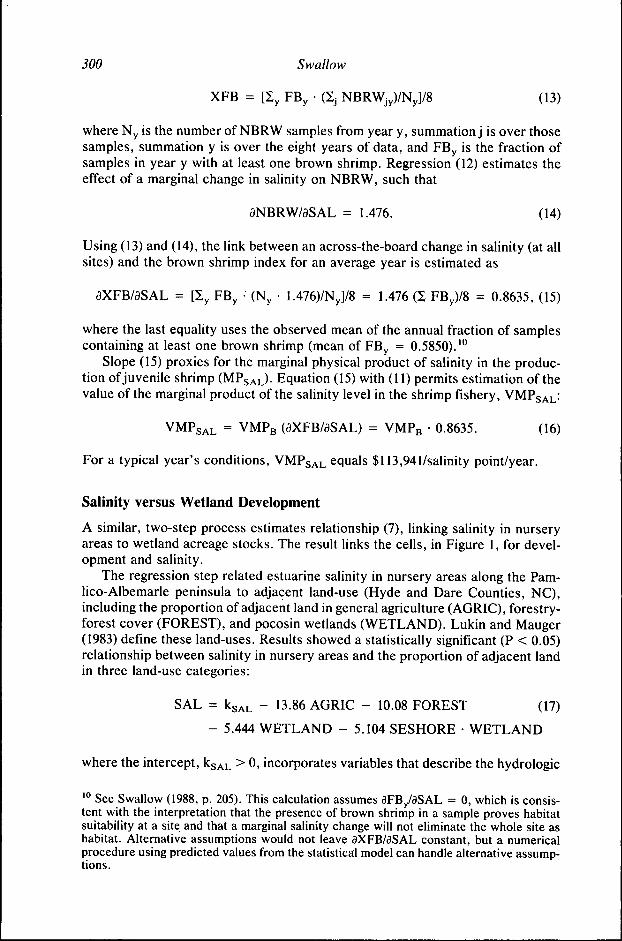
XFB = [Sy FBy • (Sj NBRWjy)/Ny]/8 (13)

where Ny is the number of NBR W samples from year y, summation j is over thosesamples, summation y is over the eight years of data, and FBy is the fraction ofsamples in year y with at least one brown shrimp. Regression (12) estimates theeffect of a marginal change in salinity on NBRW, such that

aNBRW/aSAL = 1.476. (14)

Using (13) and (14), the link between an across-the-board change in salinity (at allsites) and the brown shrimp index for an average year is estimated as

aXFB/aSAL = [Sy FBy • (Ny • 1.476)/Ny]/8 = 1.476 (X FBy)/8 = 0.8635, (15)

where the last equality uses the observed mean of the annual fraction of samplescontaining at least one brown shrimp (mean of FB = 0.5850). 10

Slope (15) proxies for the marginal physical product of salinity in the produc-tion of juvenile shrimp (MPSAL)- Equation (15) with (11) permits estimation of thevalue of the marginal product of the salinity level in the shrimp fishery,

(aXFB/aSAL) = VMPB • 0.8635. (16)

For a typical year's conditions, VMPS^L equals $113,941/salinity point/year.

Salinity versus Wetland Development

A similar, two-step process estimates relationship (7), linking salinity in nurseryareas to wetland acreage stocks. The result links the cells, in Figure 1, for devel-opment and salinity.

The regression step related estuarine salinity in nursery areas along the Pam-lico-Albemarle peninsula to adjacent land-use (Hyde and Dare Counties, NC),including the proportion of adjacent land in general agriculture (AGRIC), forestry-forest cover (FOREST), and pocosin wetlands (WETLAND). Lukin and Mauger(1983) define these land-uses. Results showed a statistically significant (P < 0.05)relationship between salinity in nursery areas and the proportion of adjacent landin three land-use categories:

SAL = ksAL - 13.86 AGRIC - 10.08 FOREST (17)

- 5.444 WETLAND - 5.104 SESHORE • WETLAND

where the intercept, ksAL > 0, incorporates variables that describe the hydrologic

'° See Swallow (1988, p. 205). This calculation assumes aFBy/SSAL = 0, which is consis-tent with the interpretation that the presence of brown shrimp in a sample proves habitatsuitability at a site and that a marginal salinity change will not eliminate the whole site ashabitat. Alternative assumptions would not leave 3XFB/aSAL constant, but a numericalprocedure using predicted values from the statistical model can handle alternative assump-tions.


Table 2Parameters for Estimating the Impact of Wetland Conversion on Estuarine

Salinity and Value of Marginal Product (VMP) of Preserving Pocosin WetlandsRather than Converting Acres to Agriculture or Forestry-Forest Land-Uses."

Conversion Impact on Salinity

Conversion of Wetlands to:

AgricultureNormal quality wetlandsHigh quality wetlands

Forestry-ForestNormal quality wetlandsHigh quality wetlands

PP

PP

Symbol

NAGR-WET

HAGR-WET

NFOR-WET

FOR-WET

Estimate

3.312*8.416*

-0.468t4.636*

S.e.

0.9361.01

0.9070.476

VMP

03

1

.282

.37

.85

Constant of proportionality(K'WET) to calculateaXFB/a WETLAND':

Normal quality wetlands (i = N) 0.4376 xHigh quality wetlands (i = H) 2.054 x

" Based on equation (17) and estimated covadances.* Significantly different from zero at P < 0.01.t Not significantly different from zero, even at P < 0.25.

conditions for the year, and dummy variable SESHORE" equals 1 for sites nearthe peninsula's southeastern shore.'^

The coefficients on the land-use variables in (17) show that converting pocosinwetlands (lowering WETLAND) to agriculture or forestry (raising AGRIC and/orFOREST) causes a net decline in the salinity of nearby shrimp nursery areas.Table 2 gives estimated parameters for the net effects on salinity. For example,converting wetlands on the southwestern shore (SESHORE = 0) to agriculturedecreases mean salinity in adjacent estuarine nurseries by 8.4 units (13.86 - 5.44;see (17) and Table 2). These results are consistent with the expectation thatsouthwestern wetlands are of "high quality" {i.e., E " ) while southeastern wet-lands are of "normal quality" (i.e., E*^).'

One can show that developing peninsular wetlands has an estimated impact on

" Southeastern shore is from longitude 75° 53' 25" W to 76° 07' 30" W.'^ See Swallow (1988, pp. 179-87, 213-19) for variable definitions and discussion of pre-liminary regressions. The standard errors for (17) are, respectively, 1.912, 1.057, 1.159,and0.7768. These estimates pertain to an equivalent GLS model which corrects for heterosce-dasticity across years of data. All variables were significant (P < 0.01) as is the model(Fi3,3oi = 439.014; P < 0.001; R^ = 0.9499; N = 315). The intercept term is given by

D79 - 13.79 D80 - 3.363 D81 - 5.118 D82(0.2481) (0.7815) (0.2713)

D84 - 1.504 D85 - 0.2170 RAIN 10 4.702 SESHORE(0.3899) (0.08329) (0.4365)

where standard errors are given in parentheses, dummy variables for each year are Dnn (nn= 1979 to 1985), and RAIN 10 is the rainfall in the ten days preceding the salinity sample.'•' Land-use variables are proportions (acreage of land-type divided by total acreage sam-pled, TOTACRE). E.g., converting 1 acre of wetlands to agriculture decreases the numer-ator of WETLAND by 1 and increases the numerator of AGRIC by 1.

= 24.81(0.7918)

- 12.40 D83 -(0.2984)

14.47(0.3650)

il.79(0.2804)

302 Swallow

the shrimp index that is proportional to the coefficients in Table 2. Doing so uses(13) and splits the summation over sampling sites j into sites near one shore ofthepeninsula (j:SESHORE -^ i; i = H,N)''* and sites away from that shore,

aXFB/aWETLAND' = (l/8)Sy{(FBy/Ny) • (18)

' + 0]}

where the zero relates to sampling sites away from that shore; and dSAhlaWETLAND' (i = H,N) is estimated from (17) (i.e., the 3s in Table 2 withSESHORE = 1 for i = N). For agricultural development, (18) simply becomes

aXFB/aWETLAND' = K'WET PSAL P'AGR-WET, i = H,N (19)

where PSAL 'S the coefficient on salinity in (12), P'AGR WET comes from (17) withTable 2, and K'^ET captures the remaining terms in (18)'^ (see Table 2).

Valuation of Pocosin Wetlands for Shrimp Fishery

By (11) and (19), the marginal value of peninsular wetlands for brown shrimpproduction is estimated by:

i = O'TT*/aXFB) OXFB/aWETLAND') (20)

• (aXFB/aWETLAND'), i = H,N;

where this annual value of marginal product is given in Table 2 for each wetlandquality and each potential land-use that wetlands displace (cf. Fig. 1). For exam-ple, the highest losses to the shrimp fishery are estimated as $3.37/acre/year fordeveloping agriculture on wetlands near the southwestern shore (Table 2). Resultsalso show that conversion to forestry-forest cover may only be a concern for highquality wetlands, from the perspective of protecting shrimp nurseries. Results fornormal quality (southeastern) pocosins remain consistent with forestry researchsuggesting that modern management may maintain the hydrologic role of thesewetlands (Campbell and Hughes 1991), but results for the high quality (southwest-ern) wetlands suggest that forestry in some locations alters wetland functions andvalues.

The estimates in Table 2 represent values for an average year based on thestatistical parameters. Table 3 provides a sensitivity analysis in the form of upperand lower bound estimates derived by using the 95% confidence bounds for eachof the three key parameters. Value estimates are most sensitive to potential es-timation error in the linkage between the shrimp index and salinity, equation (12).These bounds also show that conversion of normal wetlands to forestry-forestland-uses may cause fishery losses up to $0.22/acre-year, despite statistical insig-nificance of the impact on salinity.

''' That is, j identifies sites with one value of SESHORE and that value determines qualityindex i." For any sampling site and for the agriculture example, (aSAL/aWETLAND')j =P'AGR-WET^OTACREJ ; TOTACREj is the total acreage of land in the land-use sample nearsite j . K'wET includes i ( l ^ O T A C R E )


Table 3Sensitivity Analysis of Parameters on the Value of Marginal Product of Normal

and high (VMPH) Quality Wetlands for Protection of Salinity in BrownShrimp Nursery Areas'*

Conversion of wetlands:

To agriculture

To forestry-forest*^

Using S.E. of(equation no.)''

•9(9)

PsAL (12)PAGR-WET (1^)All three(p (9)

PsAL (12)PFOR-WET (17)All three

vUpper

0.3350.4640.4390.856

——

0.1120.218

IPN

Lower

0.2300.1000.1260.036——

-0.191—

VN

Upper

4.005.544.168.122.203.052.234.35

IPH

Lower

2.741.192.580.7431.510.6571.480.427

" Upper and lower bounds calculated using, respectively, +1.96 or -1.96 times thestandard error of estimated parameters, as indicated.

'' PsAL is the coefficient on SAL in (12); PAGR-WET and PFOR-WET are defined in Table2 using coefficients in (17). "All three" bounds are calculated using the standard errors of<P. PsAL. and either PAGR-VVET or PFOR-WET-

• Some estimates are omitted since results in (17) cause the base value of PFOR-WET < 0and PFOR-WET 'S statistically insignificant, so some bounds provide no meaningful infor-mation.

Finally, these results refute the common notion that wetlands may be valuedas a homogeneous group. The results show variation in value, despite the ab-sence, in the analysis, of a detailed accounting of the various ecological types ofpocosin wetlands (Lukin and Mauger 1983; Richardson and Gibbons 1993). Thevariation here depends not only upon geographic location, which may correlatewith ecological types, but also upon the type of developed land-use contemplated.The results illustrate that wetlands values depend not only on their role in theecosystem but also on the role that the alternative land-use would play in theecosystem.

Tradeoff Assessment and Implications

This section assesses the preservation and development tradeoffs in pocosin wet-land development by combining the empirical results with Heimlich and Lang-ner's (1986) analysis of returns to agriculture. The objective is illustrative, ratherthan prescriptive, highlighting advantages of a resource-theoretic framework anda stepwise empirical approach.

Some assumptions are necessary to adjust the available results for a resource-theoretic framework. First, on the preservation side, we assume the results forshrimp are indicative for other fisheries and that economic impacts on otherPamlico fisheries are proportional to their gross dock-side value;'^ then impacts ofsalinity or wetland changes on shrimp represent 25% of total impacts of agricul-

'* Some precedent for this type of assumption exists in Kahn and Kemp (1985); see alsoarguments in Gupta and Foster (1975).

304 Swallow

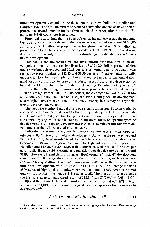
tural development. Second, on the development side, we build on Heimlich andLangner (1986) and assume returns to wetland conversion decline as developmentproceeds eastward, moving further from mainland transportation networks. Fi-nally, an 8% discount rate is assumed.

Fmpirical results show that, in Pamlico's estuarine nursery areas, the marginalloss due to an across-the-board reduction in average salinity is about $114,000annually or $1.4 million in present value for shrimp, or about $5.7 million inpresent value for all fisheries. Since policy makers (NRCD 1987) link coastal zonedevelopment to salinity reductions, these estimates justify debate over net bene-fits of development.

This debate has emphasized wetland development for agriculture. Such de-velopment annually impacts shrimp fisheries by $3.37 1986-dollars per acre of highquality wetlands developed and $0.28 per acre of normal quality wetlands, withrespective present values of $42.13 and $3.50 per acre. These estimates initiallymay appear low, but they apply to diffuse and indirect impacts. The annual mar-ginal loss is comparable to previous studies: losses from direct destruction ofhabitat for Florida blue crabs are about 0.30/acre-yr 1975-dollars (Lynne et al.1981); wetlands that mitigate hurricane damage provide benefits of 0.40/acre-yr1980-dollars {cf Farber 1987). In 1986-dollars, these comparison values are $0.44-$0.48/acre-yr. Finally, Heimlich and Langner (1986) identify pocosin developmentas a marginal investment, so that our estimated fishery losses may be large rela-tive to development values.

The stepwise empirical model offers one significant lesson. Pocosin wetlandscomprise one resource that benefits the shrimp fishery. Yet the intermediateresults indicate a real potential for general coastal zone development to causesubstantial aggregate losses via salinity. A localized focus on specific types ofdevelopment {e.g., pocosin development) may miss significant impacts from de-velopment in the full watershed of an estuary.

Following the resource-theoretic framework, we now assess the net opportu-nity cost (NOC in (4)) of agricultural development. Adjusting the per-acre wetlandvalues (Table 2) to acknowledge all Pamlico fisheries, the preservation valuebecomes $ 13.48 and $1.12 per acre annually for high and normal quality pocosins.Heimlich and Langner (1986) suggest that converted wetlands sell for $1350 peracre, while Barnes (1981) estimates acquisition and development costs around$1190. However, Heimlich and Langner (1986) estimate "typical" developmentcosts above $1500, suggesting that more than half of remaining wetlands are noteconomic for agriculture. Our illustration assumes 20% of wetlands remain eco-nomic for development, with C'(E') > 0 in (4) (i = H,N); this acreage includes2809 acres of high quality, southwestern wetlands and 11,009 acres of normalquality, southeastern wetlands (13,818 acres total). The illustration also assumesthe first acre earns an annualized return of $12.8 {i.e., rC"(2809) = 0.08 • [1350-1190]) and the return declines at a constant rate per acre so that rC'^(E'^) = 0 foracre number 13,818. These assumptions yield example equations for the returns todevelopment:"

C"(E") = 160 - 0.01158 • (2809 - E " ) (21a)

" Available data on returns to wetland conversion omit geographic location. Readers mayevaluate other assumptions at their discretion.


C' (E' ) = 127.47 - 0.01158 • (11009 - E^), (21b)

where it is assumed that the return to the last marginal unit of high quality wet-lands equals the return to the first marginal unit of normal quality wetlands; thatreturn is $10.20 annualized (0.08 times $127 present value).

In this example, the "efficient" policy would be to preserve all high quality(southwestern) wetlands because, despite their higher value for agriculture, theirvalue for fisheries is higher still and the net opportunity cost of development isnegative (N" < 0). In contrast, the policy would allow development of normalquality (southeastern) wetlands, but would halt development when the marginalnet value of development fell to an annualized $1.12 per acre (or $14 in presentvalue), where the net opportunity cost of development just equals zero (N* = 0).In this example, developers use 9800 of 11,009 acres of southeastern wetlands,leaving 1209 acres preserved.

The example compromises development and preservation interests. Develop-ers forego their most profitable wetlands because these same wetlands are mostvaluable to fisheries. However, preservationists lose 89% of the normal qualitywetlands that development threatens,'^ preserving 11%.'

Concluding Summary

A resource-theoretic approach to development and preservation tradeoffs mergesrenewable and nonrenewable resource theories, highlighting that both preserva-tion and development contribute positively to social welfare. The framework isapplied to preservation and development tradeoffs between agricultural develop-ment of pocosin wetlands and its impact on estuarine fisheries. An illustrativeassessment supports preservation of wetlands that are most attractive to bothdevelopment and fishery sectors, while development of some less highly valuedwetlands may be efficient.

Furthermore, a stepwise approach to link freshwater wetland developmentand estuarine shrimp production reveals a potential for substantial welfare lossesif estuarine salinity declines across-the-board. This result encourages research toidentify impacts of development throughout the estuarine watershed. This step-wise approach also offers a number of stages where future biophysical-economicmodels may enter the evaluation. Such fiexibility may be important as methodsfor estimation of total values improve to account for non-consumptive uses {e.g.Costanza et al. 1989; Whitehead 1993). Finally, supporting Crocker andTschirhart (1992), empirical results reveal that tracing human impacts throughecosystem linkages affects resource valuation: wetland values depend not only ontheir ecological type, but also on factors such as their geographic location and theland-use (agriculture versus forestry) in their developed state.

'* Recall the example assumes 80% of southeastern wetlands are not threatened and arepreserved by default." Given the linearity in (21) and the $160 present development value of the first acre, boththe preservation of all high quality wetlands and the proportion of normal wetlands pre-served are invariant to alternatives (e.g. 50%) to the assumption that 20% of all remainingwetlands offer positive marginal returns to development.

306 Swallow

References

Babcock, A. M. and P. R. Mundy. 1985. A quantitative measure of migratory timing ap-plied to the commercial brown shrimp fishery in North Carolina. North AmericanJournal of Fisheries Management 5(2A): 181-196.

Barnes, J. S. 1981. Agricultural adaptability of wet soils of the North Carolina CoastalPlain. Pocosin Wetlands: An Integrated Analysis of Coastal Plain Freshwater Bogs inNorth Carolina, ed. C. J. Richardson. Stroudsburg, PA: Hutchinson Ross PublishingCompany.

Batie, S. S. and C. C. Mabbs-Zeno. 1985. Opportunity costs of preserving coastal wet-lands: a case study of a recreational housing development. Land Economics 61(1): l-9>

Batie, S. S. and J. R. Wilson. 1978. Economic values attributable to Virginia's coastalwetlands as inputs in oyster production. Southern Journal of Agricultural Economics

Bell, F. W. 1986. Competition from fish farming in infiuencing rent dissipation: the craw-fish fishery. American Journal of Agricuhural Economics 68(l):95-101.

Blomo, V. J., J. P. Nichols, W. L. Griffin, and W. E. Grant. 1982. Dynamic modeling ofthe eastern Gulf of Mexico shrimp fishery. American Journal of Agricultural Econom-ics 64(3):475-482.

Brown, R. J. 1976. A study ofthe impact ofthe wetlands easement program on agriculturalland values. Land Economics 52(4):509^517.

Campbell, R. G. and J. H. Hughes. 1991. Impact of forestry operations on pocosins andassociated wetlands. Wetlands ll(Special Issue):467-479.

Clark, C. W. and G. R. Munro. 1975. The economics of fishing and modern capital theory:a simplified approach. Journal of Environmental Economics and Management 2(2):92-106.

Constanza, R., S. C. Farber, and J. Maxwell. 1989. Valuation and management of wetlandecosystems. Ecological Economics 1:335-361.

Copes, P. 1970. The backward-bending supply curve of the fishing industry. ScottishJournal of Political Economy 17(l):69-77.

Crocker, T. D. and J. Tschirhart. 1992. Ecosystems, externalities, and economics. Envi-ronmental and Resource Economics 2:551-567.

Danielson, L. E. and J. A. Leitch. 1986. Private vs public economics of prairie wetlandallocation. Journal of Environmental Economics and Management 13(l):81-92.

Epperly, S. P. and S. W. Ross. 1986. Characterization of the North Carolina Pamlico-Albemarle estuarine complex. National Oceanic and Atmospheric AdministrationNOAA Technical Memorandum NMFS-SEFC-175, U.S. Department of Commerce.

Farber, S. 1987. The value of coastal wetlands for protection of property against hurricanewind damage. Journal of Environmental Economics and Management 14(2): 143-151.

Fisher, A. C. and J. V. Krutilla. 1974. Valuing long run ecological consequences andirreversibilities. Journal of Environmental Economics and Management l(2):96-108.

Giese, G. L., H. B. Wilder, and G. G. Parker, Jr. 1985. Hydrology of major estuaries andsounds of North Carolina. U.S. Geological Survey Water-Supply Paper 2221.

Goldberger, A. S. 1968. The interpretation and estimation of Cobb-Douglas functions.Econometrica 36(3-4):464-472.

Griffin, W. L., R. D. Lacewell, and J. P. Nichols. 1976. Optimum effort and rent distri-bution in the Gulf of Mexico shrimp fishery. American Journal of Agricultural Eco-nomics 58(4 Part I):644-652.

Gupta, T. R. and J. H. Foster. 1975. Economic criteria for freshwater wetland policy inMassachusetts. American Journal of Agricultural Economics 57(l):4(>-45.

Heath, R. C. 1975. Hydrology ofthe Albemarle-Pamlico Region, North Carolina—A Pre-liminary Report on the Impact of Agricultural Development. U.S. Geological Survey,Water-Resources Investigations 9-75.


Heimlich, R. E. and L. L. Langner. 1986. Swampbusting: Wetland Conversion and FarmPrograms. Economic Research Service, Natural Resource Economics Division, Agri-cultural Economic Report No. 551, U.S. Department of Agriculture.

Hettler, W. F. and A. J. Chester. 1982. The relationship of winter temperature and springlandings of pink shrimp, Penaeus duorarum, in North Carolina. Fishery Bulletin 80(4):761-768.

Hotelling, H. 1931. The economics of exhaustible resources. Journal of Political Economy39(2): 137-75.

Jones, R. A. and T. M. Sholar. 1981. The Effects of Freshwater Discharge on EstuarineNursery Areas of Pamlico Sound. Division of Marine Fisheries, Completion Report forProject CEIP 790-11, North Carolina Department of Natural Resources and Commu-nity Development.

Judge, G. G., W. E. Griffiths, R. C. Hill, H. Llitkepohl, and T.-C. Lee. 1985. The Theoryand Practice of Econometrics, 2nd ed. New York: John Wiley & Sons.

Kahn, J. R. 1987. Measuring the economic damages associated with terrestrial pollution ofmarine ecosystems. Marine Resource Economics 4(3): 193-209.

Kahn, J. R. and W. M. Kemp. 1985. Economic losses associated with the degradation ofan ecosystem: the case of submerged aquatic vegetation in Chesapeake Bay. Journalof Environmental Economics and Management 12(3):246-263.

Kellogg, R. L., J. E. Easley, Jr., and T. Johnson. 1986. Application of a Seasonal Har-vesting Model to Two North Carolina Shrimp Fisheries. Sea Grant College ProgramPub. UNC-SG-86-03, North Carolina State University.

Krutilla, J. V. 1967. Conservation reconsidered. American Economic Review 57(4):777-786.

Lee, L.-F., G. S. Maddala, and R. P. Trost. 1980. Asymptotic covariance matrices oftwo-stage probit and two-stage tobit methods for simultaneous equations models withselectivity. Econometrica 48(2):491-503.

Loomis, J. B. 1988. The bioeconomic effects of timber harvesting on recreational andcommercial salmon and steelhead fishing: a case study of the Siuslaw National Forest.Marine Resource Economics 5(l):43-60.

Lukin, C. G. and L. L. Mauger. 1983. Environmental Geologic Atlas ofthe Coastal Zoneof North Carolina: Dare, Hyde, Tyrrell, and Washington counties. Office of CoastalManagement, CEIP Report No. 32, North Carolina Department of Natural Resourcesand Community Development.

Lynne, G. D., P. Conroy, and F. J. Prochaska. 1981. Economic valuation of marsh areasfor marine production processes. Journal of Environmental Economics and Manage-ment %{2).\15-\%(>.

Matylewich, M. A. and P. R. Mundy. 1985. Evaluation ofthe relevance of some environ-mental factors to the estimation of migratory timing and yield for the brown shrimp ofPamlico Sound, North Carolina. North American Journal of Fisheries Management5(2A): 197-209.

McCoy, E. G. 1972. Dynamics of North Carolina Commercial Shrimp Populations. Divi-sion of Commercial and Sports Fisheries, Special Scientific Report No. 21, NorthCarolina Department of Natural and Economic Resources.

NRCD 1987. Draft Source Document for the Albemarle-Pamlico Estuarine Study, 5-yearPlan. North Carolina Department of Natural Resources and Community Development,5 Feb. 1987 (unpublished manuscript).

Palmquist, R. B. and L. E. Danielson. "A hedonic study ofthe effects of erosion controland drainage on farmland values." American Journal of Agricultural Economics 71(1):55-62.

Purvis, C. E. and E. G. McCoy. 1974. Population Dynamics of Brown Shrimp in PamlicoSound. Division of Commercial and Sports Fisheries, Special Scientific Report no. 25,North Carolina Department of Natural and Economic Resources.

308 Swallow

Richardson, C. J., ed. 1981. Pocosin Wetlands: An Integrated Analysis of Coastal PlainFreshwater Bogs in North Carolina, Stroudsburg, PA: Hutchinson Ross PublishingCompany.

Richardson, C. J. and J. W. Gibbons. 1993. Pocosins, Carolina Bays, and Mountain Bogs.Biodiversity of the Southeastern United States: Lowland Terrestrial Communities,W. H. Martin, S. G. Boyce, and A. C. Echternacht, eds. New York: John Wiley &Sons, pp. 257-310.

Shabman, L. A. and M. K. Bertelson. 1979. The use of development value estimates forcoastal wetland permit decisions. Land Economics 55(2):213-222.

Skaggs, R. W., J. W. Gilliam, T. J. Sheets, and J. S. Barnes. 1980. Effect of AgriculturalLand Development on Drainage Waters in the North Carolina Tidewater Region.Raleigh, NC: Water Resources Research Institute UNC-WRRI-80-159, University ofNorth Carolina.

Stavins, R. N. 1990. Alternative renewable resource strategies: A simulation of optimaluse. Journal of Environmental Economics and Management 19(2): 143-159.

Street, M. W. and J. D. McClees. 1981. North Carolina's coastal fishing industry and theinfluence of coastal alterations. Pocosin Wetlands: an Integrated Analysis of CoastalPlain Freshwater Bogs in North Carolina, ed. C. J. Richardson. Stroudsburg, PA:Hutchinson Ross Publishing Company.

Swallow, S. K. 1988. Economically interdependent stocks and joint optimal allocation ofrenewable and exhaustible natural resources, with an application to coastal zone de-velopment. Ph.D. dissertation. Duke University.

Swallow, S. K. 1990. Depletion of the environmental basis for renewable resources: Theeconomics of interdependent renewable and nonrenewable resources. Journal of En-vironmental Economics and Management 19(3):281-296.

Tiner, R. W., Jr. 1984. Wetlands of the United States: Current Status and Recent Trends.U.S. Department of the Interior, Fish and Wildlife Service, National Wetlands Inven-tory.

Toro-Vizcarrondo, C. and T. D. Wallace. 1968. A test of the mean square error criterionfor restrictions in linear regression. Journal of the American Statistical Association63:558-572.

Waters, J. R., J. E. Easley, Jr., and L. E. Danielson. 1980. Economic trade-offs and theNorth Carolina shrimp fishery. American Journal of Agricultural Economics 62(1):124-129.

Whitehead, J. C. 1993. Total economic values for coastal and marine wildlife: Specifica-tion, validity, and valuation issues. Marine Resource Economics 8(2):119-132.

Wilen, J. E. 1985. Bioeconomics of renewable resource use. Handbook of Natural Re-source and Energy Economics, eds. A. V. Kneese and J. L. Sweeney, chapter 2.Amsterdam: North-Holland.

Williams, A. B. 1955. A contribution to the life histories of commercial shrimps (Penaei-dae) in North Carolina. Bulletin of Marine Science of the Gulf and Caribbean 5(2):116-146.

Wiser, E. H. 1983. HISARS Hydrologic Information Storage and Retrieval System User'sGuide. Raleigh, NC: Water Resources Research Institute UNC-WRRI-83-201, Univer-sity of North Carolina.

Appendix

This appendix provides details on the data and the parameters used to simulatepotential rents from the Pamlico Sound, NC shrimp fishery (Table A.I). Thismaterial will facilitate replication of the empirical results.

The empirical model treats the number of times craft landed shrimp (docked


and unloaded), N,, as one index for shrimp migratory timing based on a bioeco-nomic argument detailed in Swallow (1988, pp. 121-40). In the context of Babcockand Mundy (1985), bioeconomic support exists for using observed catch (C,.,) asa simple proxy for migratory timing since the data derive from time-invariantharvest regulations (open access).

Finally, based on Williams' (1955) life history research, the empirical analysisuses a large white shrimp index (XFW) as an indicator of prolonged high salinityconditions in nursery areas; the observed mean XFW was 0.629. If salinity is highin nurseries during summer and early fall, the survival rate of white shrimp pop-ulation will be higher. This event indicates a better year for brown shrimp pro-duction since spring salinity levels are correlated with late-season salinity levels(Heath 1975).

Catch effort data covered 1978-86, with annual series beginning in weeks17-25 and ending in weeks 48-52 (see Swallow 1988, pp. 105-6). Shrimp indicesonly covered 1979-86. Estimates in Table 1 derive from 1979-^6 data, whilemeans in Table A.I include available 1978 data. Since 1978 produced a belowaverage shrimp harvest, including 1978 in the estimate of mean conditions lowersthe estimate of rents and marginal values.

The expected price in week i, Pj (Table A.I), was estimated as a function of anational price index (available from U.S. National Marine Fisheries Service for1978-84) and shrimp size. In turn, average size was estimated as a function ofweek number and seasonal dummy variables. See Swallow (1988, pp. 140-48). For

Weekly Mean Values Used(N,, Q.,) and Ex-Vessel

Quasi-

Table A.Ito Simulate Exogenous MigratoryPrice (Pt) (December 1986-dollars

rent Equation (9) with Table 1

Timing of Shrimp, heads-ofO in

Week(t)

171819202122232425262728293031323334

No. oflandings

(N.)0.40.91.31.93.35.910.914.028.673.0138.3190.6229.6223.0198.5230.1205.0164.9

Catch(lbs)

(C.)42.711.154.6165.0320.11218.62459.93292.49860.233773.395070.4118663.1168633.6160208.0139427.2162642.7120820.193128.4

Price($/lbs)(Pt)

3.1453.2173.0783.1683.3013.2713.0573.1413.2263.3093.4093.4903.5653.6353.7183.7733.8203.857

Week(t)

353637383940414243444546474849505152

No. oflandings(NJ160.6121.8103.499.482.982.488.372.763.063.261.842.725.8ll.l10.26.42.31.1

Catch(lbs)(C.)

84325.466180.752424.346276.838719.140984.844101.033787.633343.328316.623384.812278.08410.06121.24174.72266.4742.972.1

Price($/lbs)(Pt)

3.8703.9323.9413.9403.9293.9183.4493.4143.3713.2753.2133.1503.0833.0012.9302.8542.7782.703

310 Swallow

simplicity, this study used the weekly average size of shrimp rather than disag-gregated size classes; however, statistical results were consistent with those ofKellogg et al. (1986). Furthermore, USDA indices for prices received by farmersfor hogs and for all meat animals made no statistical improvements.

For the simulation results, the intercept in Table 1 was adjusted for bias bymodifying Goldberger's (1968) procedure. This modification approximates theregression variance used by Goldberger (1968) with the sum of squares of theregression errors from the GLS model, divided by error df. The correction mul-tiplies A (Table 1) by 1.0974 and 1.0975 for models 1 and 2, respectively. While themodification is ad hoc in the presence of heteroscedasticity, omitting the correc-tion biased rents downward by >200%. (See Swallow 1988, pp. 154-56).

renewable and nonrenewable resource theory applied to

Documents