repairs and maintenance to the tax depreciation rules and maintenance to the tax depreciation rules...

Repairs and maintenance to the tax depreciation rules

An officials’ issues paper

July 2004 Prepared by the Policy Advice Division of the Inland Revenue Department and by the New Zealand Treasury

First published in July 2004 by the Policy Advice Division of the Inland Revenue Department, P O Box 2198, Wellington, New Zealand. Repairs and maintenance to the tax depreciation rules – an officials’ issues paper. ISBN 0-478-27115-8

CONTENTS

Part 1 Review of the depreciation rules 1

Chapter 1 INTRODUCTION 3

Background 4 Scope of the discussion paper 4 Principles underlying the analysis 4 Application date 13 Timeline 13 Submissions 14

Chapter 2 OVERVIEW OF THE CURRENT RULES 16

Setting economic depreciation rates 17 Pooling method of depreciation and “low-value” assets 18 Loading on economic depreciation rates 18 Special tax depreciation rates 18 Repairs and maintenance 19 Disposal of depreciable assets 19 The economic depreciation rate-setting process 20

Part 2 Structure of the rules 21

Chapter 3 ECONOMIC DEPRECIATION, ACCELERATED DEPRECIATION AND INCENTIVES TO INVEST 23

General framework 24 Investment decisions in the absence of tax 26 Investment decisions for a taxpaying individual: no inflation 27 Investment decisions of companies 30 Inflation 31 Concluding remarks 36

Chapter 4 EFFECTS OF THE CURRENT TAX DEPRECIATION RULES 38

Costs of capital 39 Calculation of economic depreciation 42 Assets with rapidly declining cash flows 44

Chapter 5 DIRECTIONS OF REFORM: STRUCTURAL ISSUES 47

Getting better depreciation rates in the absence of inflation 48 Getting better depreciation rates with inflation 55

Part 3 Specific issues 63

Chapter 6 SUGGESTED TECHNICAL CHANGES TO THE TAX DEPRECIATION RULES 65

Expenditure incurred in preventing, combating or rectifying pollution 66 When depreciation can begin for patents 70 When economic life is linked to an income-earning process or constrained by other factors (“tied assets”) 71 The special tax depreciation rate rules 73 Economic life of patents and other fixed-life intangible property 75 Plant variety rights included as depreciable intangible property 77 Clarifying the definition of “depreciable intangible property” 78 Deductibility of losses on disposal of buildings and other structures 79 Deductibility of losses on disposal of temporary buildings 82

Chapter 7 ISSUES ABOUT WHICH MORE INFORMATION IS NEEDED 83

Deductibility of asset disposal costs 83 Higher threshold for immediately deducting the cost of “low-value” assets 84

Chapter 8 CHANGES WE DO NOT AGREE WITH 86

Use of financial reporting depreciation rates for tax purposes 86 Depreciation of buildings (and other fixtures) on land held by a dealer in land 88 Treatment of property that changes use 90 Depreciation rates under the industry and asset categories 91 Difference between estimated useful life and economic life 93

Chapter 9 TAX TREATMENT OF RENTAL HOUSING 94

Background 95 Our analysis of investment in rental housing 98 Other options considered but not favoured 103

Chapter 10 ROADS, OTHER LAND IMPROVEMENTS AND “BLACK HOLE” EXPENDITURE 107

Tax treatment of roads and other land improvements 107 “Black hole” development expenditure 108

1

Part 1

Review of the depreciation rules

3

Chapter 1

INTRODUCTION

1.1 New Zealand is a small, capital importing country. If we are to make the most of our opportunities and maximise growth, capital must flow to the most productive areas of our economy. In some cases, however, the tax depreciation rules appear to be distorting investment decisions towards tax-favoured but less productive investment.

1.2 This issues paper is the result of a review of the current depreciation rules by

tax policy officials. It looks at both the problems identified and suggests legislative changes.

1.3 Part 1 of this paper introduces the issues to be discussed in the document,

outlines our goals for depreciation reform and reviews current depreciation rules.

1.4 The second part of the paper provides a framework for analysing how

depreciation provisions can affect incentives to invest, and the impact of inflation and the economic loading. We then outline possible policy reforms to address the problems we see with the current rules. Here we are asking some fundamental questions. For example, at present, most assets are depreciated smoothly over their estimated economic life to a residual value of 13.5 percent of acquisition cost. Is this a sensible way of calculating economic depreciation?

1.5 The importance of uncertainty should be stressed at the outset. The reforms

discussed in the first part do not have the impractical goal of “getting things right”. Our knowledge of how assets actually depreciate will always be too imprecise for us to have any prospect of getting depreciation rates right or even knowing if we did. The more modest goal is to avoid having depreciation rates that are too badly wrong.

1.6 The third part of the paper considers the specific issues relating to rules that

have been identified by taxpayers, their advisors and officials. The largest of these issues is the tax treatment of rental housing, although the tax issues relating to site-restoration costs are also significant.

1.7 The analysis in Part 2 of this paper, especially chapter 3, is, by necessity,

complex, although all efforts have been made to simplify the presentation where possible. It is not necessary to read chapter 3, which covers the economics of depreciation, to understand the subsequent chapters, which outline our concerns and suggestions for improvement. Even so, chapter 3 helps in the understanding of why a number of tax biases exist.

4

Background 1.8 In January 2003 the Minister of Finance announced that he had asked

officials to look at whether the present definition of “economic life” accurately reflects commercial reality. This announcement resulted in a series of submissions from taxpayers on issues of specific concern. The structure of this paper reflects our approach of addressing both the broad concern expressed by the Minister as to whether the rules were reasonable and the specific issues raised by those making submissions.

1.9 This paper also incorporates discussion on certain depreciation-related issues

have also been raised by some of the growth and innovation task forces. Scope of the discussion paper 1.10 The scope of this review is focussed on ensuring that the overall structure of

the depreciation rules is as good as is practicable and that the detailed design of our tax rules can cope with the complex, real-world issues that arise. However, this paper and the overall review by officials do not consider whether Inland Revenue has set individual rates of depreciation correctly for individual assets. Reviewing the economic life of all assets would be a very substantial task which is well beyond the scope of the current review. We judge that greater overall benefits arise if our advice to the government focuses on the wider issues we have identified. If there is a concern with a specific rate, it can be raised with Inland Revenue Adjudication and Rulings.

1.11 We are, however, interested in finding whether there are generic problems

with current depreciation economic lives. If there were widespread concerns that estimates of economic lives were dramatically wrong there would be grounds for a more general review of economic lives.

Principles underlying the analysis 1.12 Our starting point is recognition that in the absence of taxes, investment

would flow to the most productive areas of the economy, maximising our welfare. Taxes, however, can distort people’s decisions, with the result that lightly taxed activities will attract more investment, even though they have lower risk-adjusted, pre-tax returns than other investments. Correspondingly, that investment will be at the expense of investment in activities with higher risk-adjusted, pre-tax returns but which are more heavily taxed.1 The outcome is, as a society, we are poorer and we have lower growth than otherwise would have occurred.

1 This change in investment patterns will cause the returns on investing in the lightly taxed activities to fall and the returns on heavily taxed activities to rise until, on a risk-adjusted basis, after-tax returns from investing in different sectors are equalised.

5

Example Rose has $100 to invest and has a choice between two investments for a year, both with the same risk. The first investment provides a 5 percent tax-free return. The second investment provides a 7 percent return but is taxed. As Rose has a 39% tax rate, her choice is between a 5 percent after-tax return from the first investment or a 4.27 percent after-tax return from the second. She therefore chooses the first investment. In the absence of tax, she would, of course, have chosen the second investment, which had a higher return.

1.13 We are concerned about distortions in investment patterns, whether they are

accidental or deliberate. We have, therefore, included analysis on the impact of both the current depreciation rules and the “20 percent economic loading” applied to those rules.

Growth and Innovation Framework

The review of the depreciation rules has been undertaken by tax policy officials as part of the government’s formal commitment to growth and innovation. One motivation for the review has been the often expressed private sector concerns that the current tax system discourages investment in plant and machinery, especially if the investment is in areas where there is significant technical innovation. There is reason to believe that the current tax rules bias investment away from shorter-lived equipment towards longer-lived structures. Our goal is not to advantage any form of investment relative to other form of investment. Instead, the goal is to ensure tax is as neutral as possible across different forms of investment.

1.14 We conclude that unless there are important and quantifiable spill-over

benefits associated with certain forms of investment but not others, it is attractive to try to ensure that investment decisions are biased as little as possible by tax considerations.2 In effect, this means our starting point is one of making the tax depreciation provisions mirror actual economic depreciation (the fall in market value of assets) as closely as possible.3

2 A spill-over benefit is when the benefits from investment by one firm are not fully captured by that firm. For example, the benefits of an innovative investment by one firm may not be fully captured by that firm if other firms are able to copy the innovation without paying for it. 3 As is explained in chapter 3, economic depreciation would lead to the investment decisions of individuals being independent of their tax rates.

6

1.15 Even so, there is an important concern that the principles we propose applying in this area could conflict with policy goals in other areas of our tax system. By itself, a shift to economic depreciation would lead to higher tax rates on foreign equity investment in New Zealand. Excessive taxes on foreign equity investment are typically passed on to New Zealand in an economically inefficient way. At the same time, major reductions in capital taxation would narrow the base and place upward pressure on tax rates.

Summary of the issues paper

PART 1 – REVIEW OF THE DEPRECIATION RULES Introduction (Chapter 1) Chapter 1 sets out the background of the depreciation review, its scope and the principles underlying the analysis contained in later chapters. Overview of the current rules (Chapter 2) Chapter 2 outlines the current tax depreciation rules. The current rules provide a statutory deduction for depreciation for “depreciable property” (any property that might reasonably be expected to decline in value while used or available for use in deriving gross income). Depreciation rates are set by the Commissioner of Inland Revenue under a statutory formula. The formula is based on a diminishing value method (with a constant percentage of an asset’s book value allowed as a deduction), although an equivalent under the straight-line method (a constant percentage of the asset’s cost) is also typically calculated. Special rules exist for applying to the Commissioner for a depreciation rate that is higher (or lower) than the general prescribed rate (the “special tax depreciation rate” rules). A 20 percent loading applies on depreciation rates for most new assets. The majority of current depreciation rates were set as part of a comprehensive review of depreciation in 1993. PART 2 – STRUCTURE OF THE RULES Economic depreciation, accelerated depreciation, and incentives to invest (Chapter 3) Chapter 3 presents a highly stylised and simplified discussion of how taxes and different depreciation provisions can affect incentives to invest. It provides an introduction to the economics of different depreciation provisions. It starts by ignoring inflation and discusses the prima facie case for allowing economic depreciation (allowing deductions based on how assets actually fall in value) rather than more accelerated systems of depreciation. More accelerated forms of depreciation can make investments that would be unprofitable for non-taxpayers profitable to taxpayers.

7

The chapter also examines biases that can be introduced by small rates of inflation (within the Reserve Bank’s 1 to 3 percent target range). Here we discuss why if depreciation deductions did mirror how assets would depreciate in the absence of inflation, inflation can produce a bias discouraging investment in shorter-lived assets and encouraging investment in longer-lived assets. The aim of chapter 3 is to provide some background for understanding the biases that are examined in chapters 4 and 5. Readers may, if they wish, skip this chapter on an initial reading of the document. Effects of the current tax depreciation rules (Chapter 4) Chapter 4 examines how New Zealand’s current depreciation provisions, including the 20 percent loading, can affect incentives to invest. In analysing this issue, it considers a wider set of assets than were discussed in chapter 3. For reasons discussed in chapter 3, we find that the cost of capital (the minimum pre-tax rate of return at which investment is profitable) depends on the way that depreciation deductions are calculated, whether or not a loading is available and on inflation. If depreciation deductions were to mirror how assets would depreciate in the absence of inflation and there were no inflation and no loading, costs of capital would be the same for all assets. The tax system would not bias investment decisions for domestically owned firms. With small rates of inflation and no loading, there is a tax bias favouring longer-lived assets. In the absence of inflation, the depreciation loading would tend to bias investment in favour of shorter-lived assets. If inflation is in the Reserve Bank’s target range of 1 to 3 percent, however, the bias produced by the loading in favour of shorter-lived assets would be insufficient to offset the inflation-induced bias in favour of longer-lived assets. Our overall conclusion is that the loading may end up making incentives to invest more neutral than would be the case if there were no loading. This analysis is all dependent on depreciation deductions mirroring how assets would depreciate in the absence of inflation. In practice, there may be systematic biases caused by the current assumption that assets depreciate smoothly to 13.5 percent of their initial value. To our knowledge, there have been no studies of how assets actually depreciate in New Zealand. Also, the international evidence is scanty. The best international studies would suggest, however, that there are reasons to believe that the current method of calculating depreciation may be too slow for shorter-lived equipment and too fast for longer-lived structures. Finally, the chapter discusses the way in which assets with the same economic lives may have different time profiles of economic depreciation. In principle, this would provide grounds for allowing depreciation deductions to differ for assets with the same economic lives. In practice, difficulties of measurement mean that it may be impossible to take account of this complication. This means that there will inevitably be some element of “rough justice” in setting depreciation provisions.

8

Directions of reform: structural issues (Chapter 5) Chapter 5 discusses some possible structural changes to the way in which depreciation deductions are calculated. It suggests that there is a prima facie case for replacing the current assumption that assets decline smoothly to 13.5 percent of their initial value. Instead, it suggests that plant and equipment might better be depreciated on a double declining balance basis and buildings and other structures on a straight-line basis over their estimated economic lives. The double declining balance method for plant and equipment would mean that an asset with an estimated life of, say, 20 years would be depreciated as follows. Instead of allowing straight-line depreciation deductions of 5 percent per annum over the 20-year life, the asset would receive diminishing value depreciation deductions of double this rate (a diminishing value rate of depreciation of 10 percent per annum). The aim of these changes would be to better reflect how assets are actually likely to depreciate. The changes would tend to reduce depreciation deductions for buildings and other structures. For example, buildings can be currently depreciated at a diminishing value rate of 4 percent or a straight-line rate of 3 percent per annum. Shifting to straight-line deductions over a building’s estimated economic life of 50 years would involve a switch to allowing straight-line depreciation deductions of only 2 percent per annum. A diminishing value alternative with a similar present value of deductions would involve diminishing value deductions of 3 percent per annum. One concern with this approach is that it would increase depreciation deductions significantly for very short-lived equipment, and there is a lack of data on how these very short-lived assets depreciate. There is a case for obtaining more information on how they actually depreciate before changing depreciation provisions. A second concern is the limited information on how buildings and other structures depreciate. Chapter 5 also discusses possible changes to the 20 percent depreciation loading which currently applies to most assets. The current loading, while having the disadvantage of encouraging investments which might be unattractive to non-taxpayers, does have the advantage of narrowing biases between investments that different firms can undertake. However, it would be possible to reduce biases further (provided inflation remains in the Reserve Bank’s 1 to 3 percent target range) by increasing the loading for shorter-lived assets and decreasing the loading for longer-lived assets. The chapter discusses some possible approaches which will have different revenue costs. It is suggested that the final choice between these approaches should depend on revenue costs, which are still being estimated. Consistent with the goal of making incentives to invest as neutral as possible across different assets, it is also suggested that the scope of any loadings be extended to second-hand assets and used imported motorcars. This chapter also discusses other potential concerns about current depreciation provisions. It seeks comments on whether there are major generic problems with current estimates of economic lives for assets, on whether the current set of 14 depreciation bands involves too many or too few bands and on whether there are other practicable ways of better measuring how assets actually depreciate.

9

PART 3 – SPECIFIC ISSUES Suggested changes to the tax depreciation rules (Chapter 6) Chapter 6 looks at a number of technical issues where useful improvements to the current rules are possible. Deductibility of expenditure incurred in preventing, combating and rectifying pollution The rules governing deductions for capital expenditure incurred in preventing or combating pollution should be clarified. It is intended that this be done by revising section DJ 10 of the Income Tax Act 1994. It is also suggested that a deduction for site restoration expenditure be allowed in the year that this expenditure is incurred, with businesses allowed to match the cost of site restoration against income previously generated from business operations. When depreciation can begin for patents When a patent is granted, any depreciation from the time that the patent is given legal effect (when the complete application is lodged), up to the date of grant, should be allowed in the first income year in which depreciation can be claimed. Changes to the special tax depreciation rate rules A number of changes are being suggested in relation to the special tax depreciation rate rules. A key suggested change is relaxing the requirements on the Commissioner when considering special tax depreciation rate applications. This would mean that in the case of “tied” assets, for example, replacing the need for the Commissioner to be “absolutely” certain about the actual economic life of an asset with a requirement for the assessment to be only “reasonably” certain, before a special rate can be issued. Another suggested change is extending the special tax depreciation rate rules to apply to fixed-life intangible property if the Commissioner is satisfied that the actual economic life of the property will be less than its legal life. We would like further feedback on both options. We also suggest a number of technical amendments to the rules, including clarifying that the Commissioner can have regard to a broader range of factors than just the rate of depreciation adopted by the taxpayer for financial reporting purposes when considering a special tax depreciation rate application; widening the Commissioner’s ability to prescribe special tax depreciation rates using a method other than the diminishing value formula in the legislation (if such a method is more appropriate); and extending the six-month time bar on the Commissioner to consider special and provisional tax depreciation rate applications.

10

Plant variety rights included as depreciable intangible property Plant variety rights (granted under the Plant Variety Rights Act 1987) should be added to the list of depreciable intangible property in Schedule 17 of the Income Tax Act. As a clarification, the right to use plant variety rights should also be included as depreciable intangible property. Definition of “depreciable intangible property” The definition of “depreciable intangible property” should be clarified so that it is clear that property listed on Schedule 17 of the Income Tax Act can be depreciated without having further regard to whether that property can, for example, be used for tax avoidance purposes. Losses on disposal of buildings Deductions for losses on destruction of buildings as a result of natural disasters (such as the February 2004 storms, earthquake and fire) should be allowed. In principle, it would seem desirable to allow losses on voluntary destruction of buildings and losses on disposal more generally (such as losses on sale). However, we doubt whether this is practicable because of taxpayers’ scope to manipulate valuations to generate artificial losses on disposal of buildings. We consider that a loss incurred on the destruction of a “temporary building” is deductible for tax purposes, and the Income Tax Act 2004 clarifies this. Issues about which more information is needed (Chapter 7) Chapter 7 examines a number of depreciation issues about which we need further information before we can suggest changes. Deductibility of asset disposal costs Consideration should be given to full deductibility for the costs associated with disposing of depreciable assets. Currently, it is unclear whether deductions for these costs can be taken in full or are limited to the amount of any consideration derived on disposal. We would like further information on what these costs are and the circumstances in which they arise, to assist us in considering more fully the implications of such a change. Higher threshold for immediately deducting the cost of “low-value” assets A higher threshold ($2,000) for immediately deducting the cost of “low-value” assets and a higher total threshold ($20,000) for immediately deducting the cost of “low-value” assets purchased at the same time from the same supplier does not seem to be justified. This is because we do not consider that the compliance costs savings of such measures are likely to offset the significant fiscal implications. However, we would like further information on the write-off thresholds adopted for financial reporting purposes, the types of assets likely to be purchased by taxpayers at the same time and from the same supplier and the costs involved, and the potential compliance benefits from expensing versus, say, using the pool method of depreciation.

11

Changes we do not agree with (Chapter 8) Chapter 8 looks at a number of specific concerns raised by taxpayers that we do not consider should be progressed because the changes would not result in increased efficiency or are contrary to policy objectives. Use of financial reporting depreciation rates for tax purposes We do not consider that taxpayers should be allowed to use depreciation rates used for financial reporting purposes for tax purposes. This is because the Commissioner is already required to have regard to depreciation rates used by taxpayers for financial reporting purposes, both when setting general economic depreciation rates and special tax depreciation rates. The latter provides a mechanism whereby taxpayers can apply to the Commissioner for a depreciation rate that is lower or higher than that prescribed generally. Moreover, as has been discussed, we are considering extending the factors the Commissioner can consider when setting special depreciation rates. Depreciation of buildings (and other fixtures) on land held by a dealer in land The current requirement that land held by a dealer in land be treated as being held on revenue account for a period of ten years from the date of acquisition should not, in our view, be amended to allow depreciation on buildings and other fixtures constructed on the land. We do not consider that workable rules to achieve this can be devised without providing significant scope for manipulation of those rules. However, we would like feedback on any solutions that may be workable. Treatment of property that changes use We do not consider that the rules governing depreciation previously allowed in respect of depreciable assets that change use (for example, move to being held on revenue account) need clarification. The tax depreciation rules trigger a deemed disposal at market value (with the resulting loss or gain on disposal being taxable). Depreciation rates under the industry and asset categories A clarification is not needed, in our view, in relation to the process for selecting the most applicable depreciation rate in respect of an asset under the current depreciation schedules. The current tax depreciation rules already provide a number of steps for selecting the most appropriate economic depreciation rate under the industry and general asset categories.

12

Difference between estimated useful life and economic life There is no material difference between the concept of “economic life” and the term “estimated useful life”, as used in the Income Tax Act. Estimated useful life requires the Commissioner to take into account a number of factors that are relevant to the calculation of economic life, such as the impact of technological obsolescence on an asset. Tax treatment of rental housing (Chapter 9) Chapter 9 considers various aspects of the tax treatment of rental housing. We consider that there may be an element of tax advantage for investment in residential rental property and buildings more generally. Our analysis also suggests that investment in rental property may be providing a tax shelter for income from other sources. There appear to be two key ways in which these investments are tax-advantaged. First, the current method of calculating depreciation on buildings assumes that buildings depreciate smoothly to 13.5 percent of their initial value over their economic lives. We consider that this method of calculating depreciation may lead to depreciation deductions that are too quick for rental property, along with other buildings and structures. The shift to straight-line depreciation or the diminishing value equivalent for buildings and other structures examined in chapter 5 would remove this bias. The second problem is that an increasing number of residential rental property owners are claiming separate depreciation deductions for different parts of a building. Examples include separate depreciation deductions for electrical wiring, plumbing, hot water systems, carpets and internal walls. In principle, the more assets which are depreciated separately at rates that exceed the building depreciation rate, the lower the appropriate depreciation rate on the remaining shell. There is some uncertainty as to what assets can be depreciated separately, and this can lead to substantial differences in deductions claimed by two landlords with identical properties. We suggest making the rules more certain by providing landlords with two options. Under the first option, a set of separately depreciable assets would be identified, as happens in Australia. These would include lifts, domestic appliances, hot water cylinders, air conditioning systems, light fittings and carpets. However, the set of separately depreciable assets would be limited, and the remainder of the building – including wiring, plumbing and internal walls – would be depreciable at the building depreciation rate, as part of the building. This option would require taxpayers to obtain market values of these separate assets at purchase and sale to determine the tax basis for depreciation rates and to determine any gain or loss on sale. An alternative would be to depreciate all of these assets as part of the building, which would remove any need for separate valuations on purchase or sale. It would also be appropriate for taxpayers adopting this latter approach to have wider scope for deducting expenses as repairs and maintenance. For example, a replacement hot water cylinder would be capitalised and depreciated for taxpayers depreciating these assets separately, but would normally be a deductible expense for taxpayers depreciating these assets as part of the building.

13

Roads, other land improvements and “black hole” expenditure (Chapter 10) The last chapter looks at depreciation issues being considered as part of separate projects. These include the tax treatment of depreciable land improvements, primarily in the context of road construction projects, and the tax treatment of “black hole” development expenditure. The latter relates to capital expenditure that, at present, is neither deductible nor depreciable.

Application date 1.16 Given that this issues paper represents the start of the policy development

process, it is too early to include any discussion on the possible application date of any reforms. This is especially the case in relation to the suggestions in the second part of the paper, which should be thought of as longer term possibilities only. In principle, we are of the opinion that, as far as possible, any changes should not affect existing investments. However, this would add to the complexity of transitional arrangements, and submissions are invited on the issue.

1.17 There are two exceptions, however, where there are strong reasons for any

new rules to apply to investments that are in place at the application date of any new legislation. First, we are particularly concerned about the effects on investment in equipment. If faster depreciation rates for equipment are adopted, our view is that they should be available from the application date for all equipment purchased after the release of the issues paper, so that firms do not have artificial incentives to delay equipment investment.

1.18 The second exception is building fit-out for rental housing. Because some

taxpayers have been using aggressive fit-out practices, we will recommend to the government that there be no “grandfathering” in this area should the change be implemented This will not constrain the Commissioner from undertaking audit action for years prior to a change in law.

Timeline 1.19 Our intention is to report to the government on the submissions received, and

our work more generally, following the receipt of submissions. Our aim, at present, is to recommend that those more detailed measures raised in chapter 6 of this paper be included, at the earliest, in a tax bill to be introduced later this year. It is likely that the complexity of the issues raised in Part 2 and in chapter 9 will necessitate further consultation with key submitters. Measures arising from this work will, therefore, take longer. They also raise more complex issues as to fiscal cost, which will have to be considered.

14

Submissions 1.20 Specific issues for submission are addressed in the relevant chapters.

However, the key issues on which submission are requested are:

Part 2

– the general framework of our analysis;

– the conclusions as to the effect of the current rules and the economic loading, with and without inflation, presented in chapter 4;

– removing the assumption of a 13.5 percent residual value and adopting double declining balance depreciation for plant and equipment and straight-line depreciation or a diminishing-value equivalent for buildings and other structures;

– whether there are viable ways of getting better measures of economic depreciation for short-lived plant and equipment and for buildings and other structures;

– introducing an increased economic loading for short-lived assets, with a reduced loading for longer lived assets;

– whether the scope of the economic loading should be extended to include second-hand assets and second-hand imported motor vehicles.

Part 3 – the suggested amortisation provision for capital expenditure incurred in

preventing, combating or rectifying pollution and a provision allowing site restoration expenditure to be deductible against previous income;

– options to make it easier for taxpayers to apply for a special tax depreciation rate (for example, in the case of “tied” assets) and extending the special tax depreciation rules to fixed life intangible property;

– asset disposal costs – what these costs are and in what circumstances they arise;

– higher thresholds for immediately deducting the cost of “low-value” assets;

– the tax treatment of revenue account property – options for allowing depreciation of such property when the property is not purchased with the purpose or intention of resale;

– whether there are major distortions from treating the structural components of a residential rental building as a single entity; how the boundary between a building and other separately identifiable assets can be better defined; other problems with taxation of rental housing; and the other options for dealing with the taxation of rental housing which are not supported by us.

15

1.21 Submissions should be addressed to:

Depreciation Review C/- the General Manager Policy Advice Division Inland Revenue Department PO Box 2198 WELLINGTON Or email: [email protected]

1.22 The closing date for submissions is 31 August 2004 for the detailed policy

measures discussed in chapters 6, 7 and 8. This may allow them to be addressed in the taxation bill scheduled for introduction later this year. The closing date for submissions on all other matters is 30 September 2004

1.23 Submissions should contain a brief summary of their main points and

recommendations. 1.24 Please note that submissions may be the subject of a request under the

Official Information Act 1982. The withholding of particular submissions on the grounds of privacy, or for any other reason, will be determined in accordance with that Act. If you feel there is any part of your submission which you consider could be properly withheld under that Act (for example, for reasons of privacy), please indicate this clearly in your submission.

16

Chapter 2

OVERVIEW OF THE CURRENT RULES

2.1 The current tax depreciation rules, in subpart EG of the Income Tax Act 1994, provide a statutory entitlement to depreciation for all depreciable property.4 Before 1993, the legislation gave the Commissioner of Inland Revenue the discretion to allow a deduction for depreciation.

2.2 “Depreciable property” means any property which might reasonably be

expected to decline in value while used or available for use by taxpayers in deriving gross income, or carrying on a business for the purpose of deriving gross income. Depreciable property includes buildings, fixtures on land, certain land improvements, and intangible property listed in Schedule 17 of the Income Tax Act as depreciable intangible property.5 Depreciable property does not include trading stock, land, financial arrangements under the accrual rules, certain types of intangible property for which an estimated useful life cannot be calculated, such as goodwill, and property for which the cost is deductible under other provisions of the Income Tax Act.

2.3 Under the tax depreciation rules, taxpayers can elect to use either the

straight-line or diminishing value method to depreciate capital assets. Under the straight-line method, a constant percentage of the cost of the asset to a taxpayer is deducted from the property’s adjusted tax-book value. Under the diminishing value method, a constant percentage of the adjusted-tax-book value is deducted each year.6 As will be discussed in greater detail later, the Commissioner prescribes depreciation rates for use under the diminishing value method and then sets an equivalent depreciation rate for use under the straight-line method. This is achieved by ensuring, as much as possible, that the present value of the depreciation deductions under each method are equivalent.

2.4 There is also an adjustment for depreciation for the proportion of the income

year the property is owned and used or is available for use in business. So, for example, if an asset becomes available for use in a taxpayer’s business half-way through the income year, the depreciation deduction in that year will be apportioned to reflect the fact that the asset was available for use for only half the year.7

4 The current rules were the result of recommendations made by the Consultative Committee on the Taxation of Income from Capital (the “Valabh Committee”) in 1992. 5 Depreciable intangible property includes:

- the right to use a copyright; - the right to use a design or model, plan, secret formula or process, or other like property or right; - a patent or the right to use a patent; - the right to use land; - the right to use plant or machinery; - the copyright in software, the right to use the copyright in software, or the right to use software; - the right to use a trademark; - management rights and licence rights under the Radiocommunications Act 1989; - certain consents granted under the Resource Management Act 1991; and - copyright in sound recordings.

6 DV allows a larger deduction in the earlier years of the life of an asset. 7 The formula is a * b * c / 12 where a: the annual depreciation rate; b: the adjusted tax value or cost of the asset; and c: the number of months in the income year the asset was used or was available for use.

17

Setting economic depreciation rates 2.5 In setting depreciation rates for different assets, the Commissioner of Inland

Revenue must have regard to the estimated useful life of the particular asset. The estimated useful life of an asset is the time over which the asset might be expected to be useful in earning taxable income. This time must take into account factors such as the wear and tear, exhaustion, and obsolescence of an asset, as well as the period the asset is likely to be used by all its New Zealand owners. It is also based upon an assumption of normal and reasonable maintenance of the asset.

2.6 Estimated useful life focuses on the potential usefulness of a depreciable

asset to any business in New Zealand and takes into account only the effect of factors that cause the asset to depreciate. This is known as the “total life approach”. It focuses on the estimated useful life of an asset or asset class, and does not relate to a particular taxpayer. It is also consistent with the final recommendation of the Valabh Committee on Taxation.8

2.7 Estimated useful life attempts to mirror, broadly, the economic life of an

asset. This means that rates calculated by Inland Revenue are an attempt to approximate economic depreciation. Economic depreciation rates for different assets will never be able to be measured with precision, as discussed in a later chapter. The legislation refers to rates prescribed by the Commissioner as economic depreciation rates.

2.8 Economic depreciation rates are set having regard to the following legislative

formula: 1 – ((residual value / cost)(1/ estimated useful life) ) where residual value is at least 13.5% of cost. 2.9 The formula calculates diminishing value economic depreciation rates, and

Inland Revenue can then prescribe a straight-line equivalent depreciation rate.9 Economic depreciation rates are “banded” (meaning the resulting rates are rounded to the nearest band).10

2.10 Inland Revenue is required to determine economic depreciation rates for all

depreciable assets other than fixed-life intangible property, which is any depreciable intangible property that on its purchase or creation, can reasonably be expected to have an economic life which is the same as its legal life. Fixed-life intangible property must be depreciated over its legal life using the straight-line-method.

8 The Committee commented that “The definition [of estimated useful life] reflects our view that the useful life on an asset for depreciation purposes is not the life for which an asset could technically be used, but the life for which it is or will be useful in the income earning process. … it is necessary to note that it is the useful life of the asset which is the important criteria for determining depreciation rates, not necessarily the length of time for which it will be used by any particular taxpayer. This means that where an asset will be disposed of to another taxpayer for use by that taxpayer, the useful life of the asset needs to be calculated having regard to the entire period for which the asset will be used, not just the period for which the asset is first used by the taxpayer.” [letter to NZ Government of 14 November 1991] 9 See schedule 10 of the Income Tax Act 1994. 10 See schedule 11 of the Income Tax Act 1994.

18

Pooling method of depreciation and “low-value” assets 2.11 Assets valued at $2,000 or less (either costing this amount or by having been

depreciated individually to an adjusted-tax-book value equal to or less than $2,000) can be pooled and depreciated as a single asset. Taxpayers can apply to Inland Revenue to increase this maximum pooling value and can also maintain multiple pools. The depreciation rate to be used in respect of a pool is the lowest single rate applying to any asset in the pool.

2.12 The pooling method of depreciation allows assets below a certain value to be

combined and depreciated at a single rate, thereby reducing the compliance costs associated with depreciating each individual item separately (and maintaining an asset register in respect of them).

2.13 An immediate deduction is available for depreciable property costing less

than $200. This is commonly referred to as the “low-value” asset threshold. Loading on economic depreciation rates 2.14 A 20 percent loading applies to economic depreciation rates for most new

depreciable property.11 Exceptions to the loading are buildings, second-hand imported motor vehicles and fixed-life intangible property. The loading allows depreciation rates to be set at 120 percent of estimated economic depreciation.

Special tax depreciation rates 2.15 Taxpayers can apply for special depreciation rates that are higher (or lower)

than those prescribed by Inland Revenue if they consider the prescribed general depreciation rate is substantially different from the rate that should apply. This may arise, for example, if a depreciable asset is being used in a way that is different than that considered by Inland Revenue when determining a general economic depreciation rate for the asset. A special rate may also be applicable if the economic life of a depreciable asset is dependant on certain factors, such as the length of a taxpayer’s income-earning process or business (and cannot be salvaged at the end of it). However, the onus is on the taxpayer to prove that a special depreciation rate is warranted by, for example, providing evidence that an asset will cease to be useful to them or any other taxpayer after a certain date. The taxpayer is also required to provide the appropriate data to be considered by Inland Revenue.

2.16 When considering a special depreciation rate application, Inland Revenue

must have regard to the legislative formula for calculating economic depreciation rates, as well as the depreciation rate adopted by a taxpayer for financial reporting purposes.

11 Property that has not previously been used or available for use in New Zealand by any other owner.

19

2.17 Taxpayers can apply for a provisional depreciation rate for an asset if no applicable prescribed rate currently exists. This may arise in the case of newly invented assets.

2.18 Special and provisional depreciation rate applications are considered by

Inland Revenue Adjudication and Rulings. Repairs and maintenance 2.19 The cost of repairing or maintaining assets is generally treated as a

deductible expense in the year such expenditure is incurred. However, if the work adds to or improves the asset, this may constitute capital expenditure, with the cost having to be capitalised and depreciated over future years. The issue of what constitutes repairs and maintenance and what is a capital improvement can be a grey area in certain circumstances.12

Disposal of depreciable assets 2.20 A taxpayer can deduct the remaining tax-book value of a depreciable asset

(except buildings and pooled depreciable property) that is no longer used in deriving gross income or in a business. To access this write-off, the cost of disposing of the asset must exceed any consideration that would be received from its disposal.

2.21 If depreciable property is disposed of by a taxpayer for a price exceeding its

tax-book value, the excess amount (up to the asset’s original cost) is treated as gross income. This amounts to a “claw-back” of depreciation allowed on the asset. If a depreciable asset is disposed of for less than its tax-book value the difference is generally allowed as a deduction.13

2.22 Disposal of depreciable property is defined to include a change in the use of

the property, a cessation of its use in New Zealand or the loss or theft of the property. When depreciable property changes use or ceases to be used in New Zealand, the property is typically treated as being disposed of for a consideration equal to its market value.

2.23 Specific rules exist for disposal of depreciable property as a result of certain

transfers – for example, under matrimonial property agreements and between associated parties.

12 The distinction has been examined in case law – for example, in Bulcroft Main Collieries Ltd v O'Grady (1932) 17 TC 93, a replacement chimney in a factory was held to be an improvement and so capital in nature, whereas in Samuel Jones & Co (Devondale) Ltd v CIR (1951) 32 TC 513, such a chimney was held not to be an improvement and so a deductible revenue expense. In Auckland Trotting Club (Inc) v CIR [1968] NZLR 967, the case involved the reconstruction of a trotting track which the court held was a capital expenditure and not repairs to the old track. 13 A loss on disposal of buildings is not allowed as a deduction.

20

The economic depreciation rate-setting process 2.24 In anticipation of the introduction of the current tax depreciation rules in

1993, Inland Revenue conducted a comprehensive review of economic depreciation rates. The purpose of the review was to assist the department in setting economic depreciation rates, and it drew on three main sources of information: a taxpayer survey, interviews with businesses and independent valuers’ reports.

2.25 The taxpayer survey involved about 10,000 businesses from various

industries and obtained information about asset classes and data on estimated useful lives and residual market values. Respondents were asked when providing estimates to take into account expected obsolescence, exhaustion, and wear and tear.

2.26 The second main source of information was from interviews with businesses

representing different industries. Here, information was obtained about depreciation policies, asset classes and depreciation lives and rates used for financial reporting purposes.

2.27 The third source of information was independent reports from registered

valuers, who advised on the design of the asset classification system used by Inland Revenue in setting economic depreciation rates (the industry and general asset categories14) as well as estimated useful lives and residual values for different asset classes.

2.28 Since 1993 there have been minor adjustments to the economic depreciation

rates schedules, to take account of new types and categories of assets.

14 Assets peculiar to specific industries are listed and can be depreciated according to the rates set under the industry category, while assets typically used in a variety of different industries are listed in the asset category.

21

Part 2

Structure of the rules

Part 2 examines the structure of the depreciation rules. Chapter 3 provides a simplified exposition of how taxes, depreciation provisions and inflation can affect incentives to invest. This helps explain some of the biases identified in chapter 4. These biases may result in New Zealand’s investment being less productive that it might be. Chapter 5 discusses possible ways of addressing these biases.

23

Chapter 3

ECONOMIC DEPRECIATION, ACCELERATED DEPRECIATION AND INCENTIVES TO INVEST

Summary • In the absence of inflation, tax depreciation rates should equal actual economic

depreciation if they are to avoid distorting investment decisions. • Expensing of assets or accelerated depreciation can allow investments to be

profitable at pre-tax returns that are less than the pre-tax cost of borrowing. • Inflation has a significant impact on depreciating assets, especially as we use

historical cost depreciation. • For short-lived assets, historical cost depreciation is similar to nominal

economic depreciation. For long-lived assets, the current rules approximate real economic depreciation. This variation favours long-lived assets.

3.1 The prima facie case for economic depreciation may not be well understood.

For this reason, this chapter discusses the effects of economic depreciation and other possible depreciation provisions on incentives to invest.

3.2 Standard economic analysis suggests that as more and more is invested in an

activity, returns eventually get depressed. This means that measures such as accelerated depreciation that lower the cost of investment will cause investment to expand. As investment expands, returns will be bid down until it is no longer possible for firms to expand investment further.

3.3 To build up the analysis as simply as possible, this chapter initially ignores

inflation and abstracts from uncertainty. This approach allows us to examine how tax provisions can affect investment incentives as simply as possible. This is also an important case to consider. If depreciation rules would not work well in the absence of uncertainty, they will almost certainly not work well in the presence of uncertainty. Of course, it is real-world uncertainties that make measuring economic income difficult. These are at the heart of problems that will be discussed in later chapters.

24

General framework 3.4 An important policy issue is how best to minimise tax biases to investment

decisions. If taxes are not to interfere with investment decisions, it would be necessary for the investment decisions of taxpayers and non-taxpayers to be identical. As people will wish to invest if the present value of the benefits from an investment exceeds its cost, this requires that asset valuations be independent of tax rates.

3.5 For asset valuations to be independent of tax rates, economic depreciation

(the fall in market value of assets) must be deductible.15 Conversely, if assets rise in value, the accruing capital gain (the rise in the market value) would need to be taxed, irrespective of whether or not assets were sold. As will be discussed later, in the presence of inflation there is some ambiguity about how best to define “economic depreciation”. For the time being, inflation is ignored.

3.6 It should be noted that a tax system in which valuations were independent of

tax rates would not mean that taxes had no effect on investment decisions. For example, taxes are likely to affect savings and labour supply decisions, wage rates and other prices. A tax system in which asset valuations were independent of tax rates would merely ensure that, given the prices arising in the presence of taxes, taxpayers and non-taxpayers would place the same values on assets.

3.7 As we have discussed, for asset valuations to be independent of tax rates, it

would be necessary to tax accruing capital gains. In practice, there are formidable problems in taxing accruing capital gains, and even countries with capital gains taxes generally do not levy taxes on accruing gains. However, most business assets depreciate. Allowing deductions for economic depreciation for depreciating assets would, at least in theory, be a way of ensuring that, at least for these assets, investment decisions are independent of tax rates.

3.8 There are severe difficulties in measuring economic depreciation and

estimates of economic depreciation will be imprecise. This means that even if tax depreciation provisions are as close to economic depreciation as feasible, investment distortions will remain. The practical problem is how best to reform depreciation provisions, given the real-world uncertainties that exist.

15 This proposition is often referred to as the “invariant-valuations proposition”. For a formal discussion see P.A. Samuelson (1964), “The Deductibility of Economic Depreciation to Insure Invariant Valuations”, Journal of Political Economy, 72(6), 604-606. Samuelson’s article ignores uncertainty. For an extension which considers uncertainty see, G. Fane (1987) “Neutral Taxation under Uncertainty”, Journal of Public Economics, 33, 95-105.

25

3.9 A complication in analysing the effects of different possible depreciation provisions is the vast variety of revenue profiles of different possible investments. Three simple profiles that have been assumed in the economic literature are as follows: • An asset which provides a constant revenue stream for a fixed number

of periods and then expires. Such assets have constant underlying productivity through their life. For example, an asset might generate revenue of $10 per annum for each of 20 years and then expire. For such an asset, the productivity of the original investment does not deteriorate until the asset suddenly expires and is no longer used. The asset will, however, depreciate over time as its future useful life declines.

• An asset whose underlying productivity falls in a straight-line fashion for a number of periods and then expires. For example, an asset might provide revenue of $20 in year one, $18 in year two, $16 in year three and so forth, ending with $2 in year ten and then expire. Such an asset will depreciate over time more quickly than on a straight line basis as both its productivity and future life decline.

• An asset whose productivity falls in a geometric manner at some rate, δ where δ lies between 0 and 1. For example, suppose that such an asset’s productivity fell by 10 percent per annum (δ = 0.1). Suppose also that it generated revenue of $10 in year one. Then it would generate revenue of $9 ($10(1 )δ− ) in year two, $8.10 ( 2$10(1 )δ− ) in year three and so forth.

3.10 Of course, assets have a vast variety of different possible cash flows, and

even the same asset used in two different activities or by two different firms may provide substantially different cash flow profiles. A number of overseas studies have examined economic depreciation across a broad set of assets in which second-hand markets exist. The data tend to strongly reject the proposition that economic depreciation profiles are generally consistent with either of the first two types of assets. Both of these types of asset would depreciate much too slowly in early years to be consistent with the data. The third type of asset would have an infinite economic life, which clearly conflicts with the facts. This type of asset is also rejected by the data but, at least in early years, economic depreciation appears to follow a profile which is more consistent with this asset than either of the other two.16 In part as a result and in part because of the tractability of the analysis, it is extremely common for international studies to assume that cash flows take this form.

3.11 In this chapter we will illustrate key ideas as simply as possible by

considering two special polar cases of assets with geometrically declining productivity. These are as follows:

• a two period asset ( 1=δ ) which is purchased at the end of year 0 for a

fixed cost of, say, $100, which provides a single positive cash flow one year later and then expires; and

26

• a non-depreciating asset ( 0=δ ) which costs, say, $100 at the end of year 0 and provides a constant revenue stream in each future year.

Investment decisions in the absence of tax 3.12 In the absence of taxes and uncertainty, a non-taxpayer would have

incentives to keep on investing until the rate of return on further investments was driven down to the interest rate.17 Suppose that an individual can borrow or lend at the market interest rate of 5 percent and assume for the time being that there is no inflation. Table 3.1 shows cash flows for a non-depreciating marginal investment and for a two-period marginal investment. Marginal investments are investments with a zero net present value (investments where the individual ends up being just as well off as if money were deposited in a bank). A non-depreciating asset which costs $100 in year 0 and provides revenue of $5 per annum would be a marginal investment, as would a two-period investment which costs $100 in year 0 and provides $105 one year later.

Table 3.1 Non-taxpayer

Non-depreciating asset Two-period asset

Year 0 Future years Year 0 Year 1

Cost 100 Revenue 5 Cost 100 Revenue 105

3.13 If an asset costs A and provides revenue of a in each future year, its rate of

return is Aa /=ρ . Thus an asset which costs $100 and provides revenue of $5 per annum has a rate of return of 5 percent. If an asset costs A and provides revenue of a1 one year later and nothing in any future year, its rate of return is 1/1 −= Aaρ . Thus an asset which costs $100 and provides revenue of $105 one year later and nothing in any future year also has a rate of return of 5 percent because 0.05 = 105/100 – 1.

3.14 Thus, in the absence of taxes, assets would need to generate a rate of return

equal to the interest rate to make it just worthwhile for investors to hold them instead of putting their money in the bank.

16 For a discussion, see C.R. Hulten and F.C. Wykoff, 1996, “Issues in the Measurement of Economic Depreciation”, Economic Inquiry, January, 34, 1, pp. 10-23. 17 Here the analysis is on the long-run determinants of investment. In the long run, it would be expected that investment would expand until further investment would earn just the interest rate and further investment would not be profitable. In the short run, there may be many other extremely important determinants of investment including, for example, sales or the cash flow of firms.

27

Investment decisions for a taxpaying individual: no inflation 3.15 Now suppose (to keep numbers simple) that the investor is taxed at a rate of

40 cents in the dollar. So long as true economic depreciation is deductible, asset values will be independent of tax rates. Thus a marginal investment for a non-taxpayer will be a marginal investment for a taxpayer. This means that the pre-tax rate of return on a marginal investment (or the cost of capital) will still be equal to the interest rate. This is illustrated for our two polar-case investments in table 3.2, which shows that the assets with the pre-tax cash flows outlined in table 3.1 are still marginal on an after-tax basis.

Table 3.2 Economic depreciation



Cost 100 Revenue 5 Cost 100 Revenue 105

Economic Depreciation

0 Economic Depreciation

100

Tax 2 Tax 2

ATCF -100 3 -100 103 3.16 For the non-depreciating asset, true economic depreciation is zero. As in

table 3.1 it is assumed that the asset costs $100 at the end of year 0. In subsequent years taxable income will be equal to revenue of $5 minus true economic depreciation of nil. Thus $2 of tax will be paid, leaving an after-tax cash flow (ATCF) of $3. For the two-period asset costing $100, true economic depreciation in year one will be $100 because after year one the asset will be valueless, so it depreciates by $100 over the year. Thus pre-tax income in period 1 is $5 (revenue of $105 minus depreciation of $100) and tax is $2.18

3.17 Investments which are marginal for a non-taxpayer continue to be marginal

for a taxpayer provided true economic depreciation is deductible, because taxes reduce both the after-tax interest rate and the after-tax rate of return on the investment by the same proportion. The taxpayer, just like the non-taxpayer, gains exactly the same after-tax cash flows from these assets as could be obtained by depositing $100 in a bank.

3.18 There is nothing special about the particular examples we have chosen. If

true economic depreciation is deductible, investments which are marginal for a non-taxpayer will be marginal for taxpayers on any tax rate.

18 These examples are clearly stylised and the two-period example ignores the possibility of part-year depreciation in year 0. In principle, if an asset did provide a single positive cash flow, the asset would not depreciate until the time when this cash flow is derived so no depreciation deduction should be allowed until this time. In practice, allowing part-year depreciation deductions is likely to be broadly appropriate when assets provide revenue continuously throughout an income year rather than at a single point in time.

28

Effect of expensing and scope for tax arbitrage 3.19 If tax depreciation is faster than economic depreciation, this will drive down

the pre-tax rate of return on marginal investments below the interest rate. An extreme but easy case to analyse is that of immediate deductibility or expensing. In this case, provided the investor’s tax rate remains the same in each future year, the cost of capital will be equal to the after-tax interest rate. This is illustrated in table 3.3, where it is shown that if the interest rate remains 5 percent, investments earning a pre-tax rate of return of 3 percent become marginal.

3.20 For both the non-depreciating and the two-period asset, the $100 of

expenditure in year 0 leads to a tax saving of $40, so the after-tax cost in year 0 is $60. If the non-depreciating asset provides revenue of $3 per annum (a 3 percent pre-tax rate of return), this will lead to a tax liability of $1.20 in each subsequent year and hence an after-tax cash flow of $1.80. This is exactly equal to the after-tax interest the investor would receive if $60 were placed in a bank account earning 5 percent interest, which would provide $3 per annum of pre-tax interest rate and $1.80 of after-tax interest. Similarly, for the two-period asset, an investment with a 3 percent pre-tax rate of return is marginal on an after-tax basis.

3.21 There are several reasons for this result:

• Irrespective of depreciation provisions, there will always be incentives to invest until the after-tax rate of return is bid down to the after-tax interest rate, which is 3 percent in this example.

• Provided tax rates remain constant, expensing leads to after-tax costs and revenues falling in the same proportion. This means that the pre-tax rate of return will be equal to the post-tax rate of return.

• Thus, in equilibrium, the pre-tax rate of return on a marginal investment will equal the after-tax interest rate.

Table 3.3 Expensing



Cost 100 Rev 3.0 Cost 100 Rev 103.0

Deprec 100 Deprec 0.0 Deprec 100 Deprec 0.0

Tax Saving

40 Tax 1.2 Tax Saving

40 Tax 41.2

ATCF -60 1.8 ATCF -60 61.8

29

3.22 The preceding analysis leads to an obvious concern with expensing (or, to a lesser extent, with other accelerated depreciation measures). In the absence of taxes, borrowing (or reducing lending) at a 5 percent interest rate to invest at a 5 percent rate of return is marginal. With economic depreciation and a tax rate of 40 percent, borrowing at 5 percent to earn 5 percent is still marginal. However, with expensing, borrowing at 5 percent to earn 3 percent becomes marginal. It becomes profitable for investors to invest at a lower rate of return than the interest rate because investments are effectively subsidised by the tax system.

3.23 Economic depreciation leads to similar incentives to invest for both

taxpayers and non-taxpayers. By contrast, taxes and accelerated depreciation can provide taxpayers with incentives to invest in cases where investment would be unprofitable for a non-taxpayer.

3.24 Not only is there the obvious inefficiency associated with encouraging the

economy to borrow on world capital markets at 5 percent to invest at 3 percent, but there is also the potential problem of tax arbitrage. Suppose that the interest rate is 5 percent but that real assets earn 3 percent. Those on tax rates lower than 40 percent will have incentives to lend rather than investing directly in real assets. When this happens, negative amounts of tax can be collected on investment income.

3.25 To illustrate this, consider the case of a tax-exempt charity which has $60

which it could invest in a proportionately scaled-down version of the non-depreciating asset described on the left-hand side of table 3.3. If it were to do so, it would earn tax-free revenue of $1.80 per annum, providing a 3 percent return on its investment. Instead, however, it lends the money to a 40 percent marginal rate taxpayer who invests in $100 of the real asset. The $60 borrowed, together with the tax saving of $40, allows $100 of real asset to be acquired. In future years, income from the asset will balance the interest expense and there will be no tax to pay. Thus in year 0 this investment reduces taxes paid by $40 without any offset in future years, so the investment is negatively taxed.

3.26 This is shown in table 3.4. On the left-hand side we record cash flows from

the 40 percent marginal rate taxpayer’s perspective. In year 0 the cost of the asset is financed by borrowing $60 and a tax saving of $40, leaving an after-tax cash flow of $0. In future years, revenue from the asset balances the interest expense, leading to a zero tax liability and an after-tax cash flow of $0. From the government’s perspective, $40 is lost in year 0 without any offsetting future gain.

3.27 These tax arbitrage opportunities mean that a business income tax base with

heavily accelerated depreciation provisions can end up collecting negative amounts of revenue.

30

Table 3.4 Expensing and tax arbitrage

Taxpayer’s perspective Government’s perspective

Year 0 Future years Year 0 Future years

Cost 100 Revenue 3.0 Tax -40.0 0.0

Deprec 100 Deprec 0.0

Tax Saving

40 Interest Expense

3.0

Borrowed Funds

60 Tax 0.0

ATCF 0.0 0.0 3.28 The analysis so far has considered the cases of economic depreciation and of

immediate expensing as an example of accelerated depreciation. Now consider the opposite case, where tax depreciation is too slow. This can result in capital investment being taxed and the cost of capital rising above the interest rate. For an extreme example, consider the case of a two-period asset, but this time assume that no depreciation is allowed for tax purposes. Once more, assume that $100 is invested in year 0 and the interest rate is 5 percent per annum. A taxpayer on a 40 percent marginal rate would need to earn $103 after tax to be as well off as by putting money in the bank. This would require pre-tax revenue of $171.67 = $103/(1 – 0.4), or a real pre-tax rate of return of 71.67 percent. This would clearly discourage investment with higher pre-tax returns than the 5 percent cost of funds to the economy. Failure to allow economic depreciation for assets which do depreciate is likely to be very inefficient.19

Investment decisions of companies 3.29 By themselves, the previous examples would appear to suggest a strong case

for eliminating any element of accelerated depreciation and ensuring that tax depreciation is neither faster nor slower than economic depreciation. The preceding analysis has applied to investment by unincorporated enterprises owned by New Zealand residents. Qualitatively similar results would hold for investment by companies owned solely by New Zealand residents. This is because under the New Zealand full imputation scheme, distributed income ends up being taxed once at the marginal tax rates of shareholders. By itself, this bolsters the case for economic depreciation.

19 Of course, this is likely to bias decisions on who undertakes investment. For example, if there were heavily taxed investments earning 71.67 percent when the interest rate was 5 percent, there would be strong incentives for non-taxpayers to invest in such assets rather than lending.

31

3.30 There is, however, a very important balancing consideration. New Zealand currently allows accelerated depreciation through a 20 percent loading on depreciation rates for plant and equipment. Removing accelerated depreciation provisions would boost effective tax rates on foreign direct investment and foreign portfolio equity investment, which would discourage foreign equity investment. This is of concern because taxes on foreign equity investors could ultimately be borne by domestic residents but in a more costly way than if domestic residents were taxed directly.

3.31 The key problem is that depreciation deductions provide one instrument for

addressing two quite separate problems. An across-the-board move to eliminating any element of accelerated depreciation could increase the efficiency of investment decisions for firms that are operated in the interests of domestic resident shareholders, but decrease the efficiency of investment decisions for firms that are operated in the interests of foreign shareholders. Of course, there may be better ways of addressing concerns about foreign equity investment in New Zealand than through the size of depreciation deductions. Work on such issues, however, is beyond the scope of the current depreciation review.

Inflation 3.32 Now we once more consider investment by an unincorporated enterprise

owned by an individual on a 40 percent marginal tax rate but this time examine how modest levels of inflation can affect the analysis. We assume a 2 percent inflation rate, which is in the middle of the Reserve Bank’s target range. We assume that inflation has no effect on the real interest rate faced in New Zealand, so the nominal interest rate rises in line with inflation. We also assume that inflation of 2 percent per annum means that all prices rise at this rate. In practice, the cost to consumers of inflation is smaller than the measured inflation rate because of the way in which consumers can substitute towards goods and services whose relative price declines.

3.33 Minor levels of inflation will have two effects on investment. First, provided

changes in inflation do not affect the real interest rate, they will tend to boost the subsidy conferred by accelerated depreciation. Second, if depreciation rates were set to mirror how assets would depreciate in the absence of inflation, they would tend to produce a bias favouring longer-lived investments over shorter-lived investments.20

20 This is well known. For example, the United States Treasury, Report to Congress on Depreciation Recovery Periods and Methods, July 2000 (page 48) states, “All else equal, an unindexed tax system favours investment in long-lived over short-lived assets.” An early reference is Auerbach, A.J., 1979, “Inflation and the Choice of Asset Life”, Journal of Political Economy, 87(3), 621-638.

32

3.34 With a real interest rate of 5 percent per annum and an inflation rate of 2 percent the nominal interest rate will be 7.1 percent.21 The real after-tax interest rate will be approximately 2.22 percent.

3.35 First, consider the case where capital expenditure can be expensed (the

easiest case to consider). In this case, the real pre-tax rate of return on a marginal investment will be bid down to the real after-tax interest rate of 2.22 percent, compared with 3 percent in the absence of inflation. Thus inflation reduces the cost of capital. Borrowing at a real interest rate of 5 percent to earn a real pre-tax rate of return of 2.22 percent becomes marginally profitable.

3.36 Table 3.5, which can be compared with table 3.3, records the real (inflation

adjusted) cash flows generated on the two types of asset. 3.37 Consider first the two-period asset. The asset costs $100 in year 0 and

provides real revenue of $102.22, or nominal revenue of 02.122.102$26.104$ ×= in year one. On an after-tax basis the asset costs

$60 and provides an after-tax real cash flow of $61.33, or nominal cash flow of 02.133.61$56.62$ ×= in year one. The investor ends up exactly as well off as if $60 were placed in a bank for a year.

Table 3.5 Inflation and expensing



Cost 100 Revenue 2.22 Cost 100 Revenue 102.22

Deprec 100 Deprec 0.00 Deprec 100 Deprec 0.00

Tax Saving

40 Tax 0.89 Tax Saving

40 Tax 40.89

ATCF -60 1.33 ATCF -60 61.33 3.38 The non-depreciating asset costing $100 in year 0 will provide real revenues

of $2.22 in each subsequent year. This is equivalent to nominal revenues of $2.26 = 02.122.2$ × in year one, 202.122.2$31.2$ ×= in year two and so forth. Again, the taxpayer ends up just as well off as if $100 were deposited in a bank account and additional deposits were made at the end of each year to maintain the real value of the deposit.

21 If r denotes the real interest rate, π the inflation rate and i the nominal interest rate, the relationship between the real and nominal interest rate is given by )1)(1(1 π++=+ ri or ππ ++= )1(ri or, conversely, ]1/[][ ππ +−= ir . With a tax rate, m, the after-tax real interest rate will be ]1/[])1([' ππ +−−= mir .

33

3.39 The more complex case to consider is that of economic depreciation. In times of inflation there are a number of ways in which economic depreciation might be defined. For asset values not to depend on tax rates, so long as nominal interest income is taxed and nominal interest expense is deductible, it would be necessary to allow a deduction for the fall in the nominal market value of assets (and to tax accruing nominal gains). We will refer to this as “nominal economic depreciation” or NED). If nominal economic depreciation is deductible (and nominal gains are taxed as they accrue), we say that an asset is being taxed on its full “nominal economic income”. Economists have more often used the words “economic depreciation” to mean the fall in the real market value of assets. We will use the words “real economic depreciation”, or “RED”, to refer to this definition of economic depreciation. If real economic depreciation were deductible (and real gains taxed on accrual), we say that an asset is being taxed on its “real economic income”.

3.40 In practice, the way that Inland Revenue computes rates of economic

depreciation for most assets takes no account of inflation at all. Its method of calculating depreciation seems more likely to provide an extremely rough proxy for the way in which assets might depreciate if there were no inflation. We will refer to such a measure as “historical cost approximation for economic depreciation” or “HCA”.

3.41 To see the difference between these measures, consider an asset which in the

absence of inflation would be worth $200 at the end of year 0, $100 at the end of year one and $0 at the end of year two. Suppose, however, that there is 2 percent inflation each year so the asset is worth $200 at the end of year 0, $102 at the end of year one and $0 at the end of year two. Nominal and real values of nominal economic depreciation, real economic depreciation and the historical cost approximation over years one and two are recorded in table 3.6.

Table 3.6 Possible depreciation deductions with 2 percent inflation

Nominal asset values Nominal values Real values

Year 0=π 02.=π NED HCA RED NED HCA RED

0 200.0 200.0

1 100.0 102.0 98.0 100.0 102.0 96.1 98.0 100.0

2 0.0 0.0 102.0 100.0 104.0 98.0 96.1 100.0

34

3.42 Consider first the middle set of columns, “nominal values”. If nominal economic depreciation were deductible, the taxpayer could deduct $98.0 in year one (the fall in the asset’s nominal value from $200 to $102) and $102 in year two. Under the historical cost approximation, $100 would be deductible in each of years one and two. This measures how the asset would depreciate in the absence of inflation. To calculate real economic depreciation in year one, the taxpayer would be allowed to subtract the current value of the asset ($102) from its inflation-adjusted acquisition cost ( 02.1200$204$ ×= ). This would leave the asset with a book value of $102 at the end of year one. Likewise, in year two the taxpayer could deduct the current value of the asset (viz., $0) from its inflation-adjusted book value ( 02.1102$104$ ×= ). The final three columns give the real (inflation-adjusted) value of these deductions.

3.43 It might be observed that in the simple example in table 3.6 there is little

difference between the present value of depreciation deductions under nominal economic depreciation and the historical cost approximation, but there is a bigger difference between the historical cost approximation and real economic depreciation. This will generally be the case for short-lived assets such as the three-period example in table 3.6. By contrast, for very long-lived assets, the historical cost approximation will be much closer to real economic depreciation than to nominal economic depreciation.

3.44 Although a switch to a nominal economic income base is not being

suggested, it is worthwhile thinking through the implications of both a nominal economic and a real economic income base. This helps in understanding the effects of the historical cost approximation. At one polar extreme (the two-period asset), the historical cost approximation will result in nominal economic income being taxed. At the other polar extreme (the non-depreciating asset), the historical cost approximation will result in real economic income being taxed.

Nominal economic income base 3.45 If nominal economic depreciation was deductible for all assets and nominal

gains taxed as they accrued so assets were taxed on their full nominal economic income, the cost of capital for all investments would be equal to the real interest rate, which is 5 percent in our examples. This is illustrated in table 3.7. Consider first the two-period asset, which generates real revenue of $105 in year one (a real pre-tax rate of return of 5 percent). The nominal depreciation deduction in year one would be $100 and the real value of this deduction would be $98.04 ($100/1.02). The real tax payment would be $2.78 (40 percent of [$105 minus $98.04]). The investor would earn a real after-tax rate of return of 2.22 percent, which equals the after-tax real interest rate of 2.22 percent derived earlier.

35

Table 3.7 Nominal economic depreciation



Cost 100 Rev 5.00 Cost 100 Rev 105.00

Cap Gain 1.96 Deprec 98.04

Tax 2.78 Tax 2.78

ATCF -100 2.22 ATCF -100 102.22 3.46 Now consider a non-depreciating asset which generates real revenues of $5

per annum (a real pre-tax rate of return of 5 percent). In year one the asset will generate a nominal capital gain of $2, which is $1.96 ($2.00/1.02) in real terms. The real tax liability would be $2.78 (40 percent of $5.00+$1.96). The real after-tax cash flow will be $2.22. In future years, real tax liabilities and real after-tax cash flows will be the same, so the taxpayer will end up earning an after-tax rate of return of 2.22 percent, which is once more equal to their required after-tax real interest rate. Thus these investments earning a 5 percent real pre-tax rate of return are marginal on an after-tax basis.

3.47 Under a comprehensive nominal economic income base, all investment

returns would be taxed on the same basis as interest. This is why the cost of capital does not depend on tax rates in this case.

Real economic income base 3.48 If real economic depreciation was deductible for all assets and real gains

taxed as they accrued so assets were taxed on their real economic income, the cost of capital for all investments would be equal to 3.70 percent. This means that the real post-tax rate of return will be equal to 3.70%×(1-0.4)=2.22%, which would be the real after-tax interest rate that investors demand. This is illustrated in table 3.8.

3.49 First consider the non-depreciating asset. As this asset does not depreciate in

real terms, real economic depreciation is zero in each year. Investors need to earn a 2.22 percent real after-tax return to be as well off as they would be from earning interest. The asset needs to provide pre-tax real income of $3.70 or $2.22/(1-0.4) to be as attractive on an after-tax basis as interest.

3.50 Now consider the two-period asset. If this provides real revenue of $103.70

in year one, and benefits from a real depreciation deduction of $100 in that year, the investor will earn a real after-tax cash flow of $102.22 in that year, which is as good as could be derived by putting money in the bank.

36

Table 3.8 Real economic depreciation



Cost 100 Rev 3.70 Cost 100 Rev 103.70

Deprec 0.00 Deprec 100.00

Tax 1.48 Tax 1.48

ATCF -100 2.22 ATCF -100 102.22

Historical cost approximation 3.51 Finally, consider the historical cost approximation. For the two period asset

a nominal deduction of $100 (a real deduction of $98.04) would be allowed in year one. This is exactly the same as would be allowed under a nominal economic income base. It is less generous than allowing for inflation indexed depreciation deductions as would be provided under a real economic income base.

3.52 By contrast, consider the non-depreciating asset. In the absence of inflation,

this would neither appreciate nor depreciate, so under the historical cost approximation, there would be neither depreciation deductions nor capital gains taxation. However, this is the treatment that would be afforded under a real economic income base. It is more generous than would be afforded under a nominal economic income base, under which nominal capital gains would be taxed.

3.53 Thus, under the historical cost approximation, there is a built-in bias

favouring long-lived relative to short-lived assets. At the extreme, for two-period assets, both the real and the inflationary component of income are taxed, whereas for a non-depreciating asset only the real component of economic income is being taxed. This insight is important in understanding the tax biases analysed in chapter 4.

Concluding remarks 3.54 Even in the absence of inflation, the best way of calculating depreciation

provisions is a complex issue. If there were no foreign equity investment in New Zealand, there would be strong grounds for attempting to eliminate accelerated depreciation and getting depreciation deductions as close to economic depreciation as possible. This would minimise tax biases to investment decisions. However, by itself, removing accelerated depreciation provisions would boost taxes on foreign equity investment in New Zealand in ways which are likely to be undesirable.

37

3.55 Inflation, together with historical cost depreciation, creates an additional complication. Even if depreciation deductions were to measure accurately how assets would depreciate in the absence of inflation, allowing historical cost deductions would introduce biases in the presence of inflation. These would favour long-lived relative to short-lived investments.

3.56 A problem to be discussed in chapter 4 is that the current method of

calculating depreciation provisions seems arbitrary and may not be the best way of calculating economic depreciation, even in the absence of inflation.

3.57 The reforms discussed in this paper are aimed at reducing biases to

investment decisions without increasing overall taxes on capital income.

38

Chapter 4

EFFECTS OF THE CURRENT TAX DEPRECIATION RULES

Summary • There are two ways in which current depreciation provisions may bias

investment away from shorter-lived equipment towards longer-lived structures. • This is an intrinsic feature of a system of historical cost depreciation in the

presence of inflation. • It may be reinforced by the way that depreciation deductions are calculated

using an assumed 13.5 percent residual balance. This chapter explores how inflation can affect costs of capital and examines biases that can be introduced by the 13.5 percent residual balance formulation.

4.1 In chapter 3, we discussed how in the absence of inflation and uncertainty, economic depreciation would lead to the cost of capital (or minimum pre-tax rate of return at which investment becomes profitable) for an unincorporated enterprise being set equal to the interest rate. We also examined how accelerated depreciation or inflation could lead to costs of capital being driven down below the real interest rate. To present the analysis as simply as possible, we considered two polar cases: a two-period asset and a non-depreciating asset.

4.2 This chapter examines how current tax rules and inflation affect incentives to

invest in a wider set of cases. To start with, we make the assumption that rates of depreciation allowed for tax purposes would mirror economic depreciation in the absence of inflation. In practice, there are grounds for querying whether current depreciation provisions do provide a good proxy for economic depreciation but we ignore this issue initially. We start by also ignoring the 20 percent loading to depreciation rates available for most assets and calculate costs of capital in the absence of any loading. We then extend the analysis to take account of the 20 percent loading.

4.3 The current method of calculating depreciation may not be the best way of

calculating economic depreciation. The normal method of calculation uses estimates of economic life. A rate of diminishing value depreciation is calculated on the assumption that an asset’s value is 13.5 percent of its acquisition cost at the end of its economic life. The chapter discusses the appropriateness of this method of calculating economic depreciation.

4.4 Assets with the same economic life may have very different cash flow

profiles. Implications for economic depreciation are also examined.

39

4.5 This chapter focuses on the effects of current depreciation provisions. Chapter 5 will examine directions for possible reforms.

Recognition of impact of uncertainty and variability on analysis

Our analysis abstracts from many factors, such as the impact of the business cycle or exchange rates on asset valuations, which, in the practical world, may have a more significant effect on the accuracy of depreciation for taxpayers than some of the issues which concern us in this paper. The variability of inflation must affect how successful our suggestions to address the impact of inflation will be. Even if the Reserve Bank keeps CPI inflation within the 1 percent to 3 percent range, the volatility of individual asset prices can obviously be much greater.

Nevertheless, we consider that, to the extent problems can be identified with the current rules, we should attempt to address them while still recognising that real-world uncertainties exist.

Costs of capital 4.6 Suppose that assets provide revenues that decline at a geometric rate δ . For

example, if 0.1δ = and an asset provides $10 at the end of year one, it provides $9 at the end of year two, $8.10 at the end of year three, $7.29 at the end of year four and so forth. The two-period asset, discussed in chapter 3, can be considered as the special polar case where 1δ = and the non-depreciating asset as the special polar case where 0δ = . Here we extend the analysis to allow for other possible cases.22

4.7 Table 4.1 outlines estimates of costs of capital (the minimum pre-tax rate of

return at which investment becomes profitable) for an unincorporated enterprise in the absence of any loading, assuming that Inland Revenue’s estimated rates of depreciation (without the loading) would mirror economic depreciation in the absence of inflation.23 This is a strong assumption which will, at best, be an approximation to the truth. This means that investment biases are likely to be larger than analysed later. We assume that taxpayers adopt the diminishing value basis for depreciation and consider only assets with depreciation rates in the midpoint of a banded depreciation rate. Again, this will tend to understate depreciation biases.

4.8 In practice, inflation will be uncertain and variable. We abstract from this

complication and assume a constant, perfectly anticipated rate of inflation. A real interest rate of 05.0=r and a tax rate of 39.0=m are also assumed.

22 A further assumption is that so long as δ is less than 1, assets are never retired from service.

23 The cost of capital is given by ( ) ( )1 '

1mZ r

mδ

ρ δ− +

= −−

where m is the taxpayer’s marginal tax rate (assumed to be 39

percent in each period), Z is the present value of depreciation deductions, per dollar of investment, and r’ is the real after-tax cost of funds. Exactly the same formula arises if, rather than assuming that assets provide a single cash flow each year, they are assumed to provide cash flows continuously throughout each year.

40

Table 4.1 Costs of capital: unincorporated enterprises – no loading

Inflation rate

Depreciation rates 0.00π = 0.01π = 0.02π = 0.03π =

0.50 5.00 4.98 4.95 4.92

0.33 5.00 4.96 4.90 4.84

0.22 5.00 4.93 4.84 4.73

0.18 5.00 4.91 4.80 4.67

0.15 5.00 4.89 4.76 4.61

0.12 5.00 4.87 4.71 4.52

0.075 5.00 4.81 4.58 4.31

0.06 5.00 4.77 4.51 4.21

0.04 5.00 4.71 4.37 4.01

0.02 5.00 4.60 4.16 3.70

0.00 5.00 4.37 3.75 3.14 4.9 In the absence of inflation, the cost of capital for all forms of investment

would be equal to the interest rate, in line with the discussion in chapter 3. We saw in chapter 3 that in the presence of inflation, costs of capital remain equal to the real interest rate if 1=δ (the asset is a two-period asset). This is because the full nominal economic income from such an asset is being taxed on the same basis as interest.

4.10 For assets depreciating at a diminishing value rate of 50 percent per annum,

costs of capital are close to the real interest rate of 5 percent. In other cases, costs of capital fall because assets are taxed on less than their full nominal economic income. At a 2 percent inflation rate )02.0( =π , the cost of capital for a non-depreciating asset ( 0=δ ) is 3.75 percent.

4.11 Most assets used in New Zealand other than buildings qualify for a 20

percent depreciation loading. For non-depreciating assets a depreciation loading is clearly of no benefit. For depreciating assets, the depreciation loading increases the present value of depreciation deductions, which reduces the cost of investment and the cost of capital.

4.12 Table 4.2 considers the case of the depreciation loading. The 20 percent

loading would have no effect on incentives to invest in non-depreciating assets but would increase incentives to invest and lower costs of capital for depreciating assets. In the absence of inflation, costs of capital would fall most for assets which depreciate faster.

41

Table 4.2 Costs of capital: unincorporated enterprises – 20% loading

Inflation rate

Depreciation rates 0.00π = 0.01π = 0.02π = 0.03π =

0.50 4.69 4.61 4.54 4.45

0.33 4.70 4.61 4.51 4.40

0.22 4.71 4.60 4.47 4.34

0.18 4.72 4.59 4.45 4.30

0.15 4.72 4.59 4.43 4.25

0.12 4.73 4.58 4.40 4.20

0.075 4.76 4.55 4.32 4.06

0.06 4.77 4.54 4.27 3.98

0.04 4.80 4.52 4.19 3.84

0.02 4.86 4.47 4.05 3.60

0.00 5.00 4.37 3.75 3.14 4.13 In the absence of inflation, there would appear to be two unattractive features

of the depreciation loading. First it tends to subsidise investment, encouraging investments at lower pre-tax rates of return than would be profitable for a non-taxpayer. This encourages investment that earns lower pre-tax rates of return than the cost of funds to the economy. Secondly, it favours faster-depreciating relative to slower-depreciating assets. Investment in faster-depreciating assets may displace investment in slower-depreciating assets merely because of a relative tax advantage.

4.14 At higher rates of inflation, however, our estimates suggest that the loading

only partially offsets the bias caused by inflation. Costs of capital are lowest for assets which depreciate most slowly. The loading may have the unattractive feature of increasing investment subsidies. For example, at an inflation rate of 2 percent per annum and with a depreciation rate of 0.5, the cost of capital falls from 4.95 percent to 4.54 percent as a consequence of the depreciation loading. At the same time, however, the loading reduces the spread of costs of capital. At an inflation rate of 2 percent per annum, costs of capital would vary between 3.75 percent and 4.95 percent in the absence of any loading but only vary between 3.75 percent and 4.54 percent in the presence of the loading. This means that if inflation is in the Reserve Bank’s target range, the loading may reduce investment biases.

42

4.15 The figures in table 4.2 suggest that capital investment by unincorporated enterprises in New Zealand is under-taxed, not over-taxed. Similar results are likely to emerge if the analysis is extended to consider the case of companies owned solely by New Zealand residents. However, for companies owned solely by foreign non-resident equity investors, the opposite conclusion can emerge. In this case, the depreciation loading may reduce excessive taxes on foreign equity investment while, at the same time, reducing biases between investments of differing durability.

4.16 Because depreciation allowances affect incentives to invest for both

domestically owned and foreign-owned firms, there is some genuine uncertainty as to whether a change to the rules which increased costs of capital without changing their variability would be in the country’s best interests. However, measures which reduce variability of costs of capital without changing average costs of capital would appear desirable.

4.17 A key concern of the depreciation review is whether or not there are likely to

be practical reforms which work in this direction. One such step might be to increase capital write-off provisions for shorter-lived assets while reducing them for longer-lived assets. Chapter 5 explores how this sort of measure might be used to improve the neutrality of investment decisions. This sort of measure might lead to a small but nonetheless noticeable improvement in neutrality.

Calculation of economic depreciation 4.18 So far, it has been assumed that tax depreciation, ignoring the 20 percent

loading, would mirror economic depreciation in the absence of inflation. 4.19 The current way economic depreciation is estimated for assets which are

likely to have a residual value at the end of their economic life, T, of less than 13.5 percent of their acquisition cost is to assume that the diminishing value rate of depreciation is δ where 135.0)1( =− Tδ . The diminishing value depreciation rate is rounded to the nearest banded rate. Taxpayers have the option of adopting the diminishing value depreciation rate or a slower straight-line rate. The straight-line rate is chosen to lead to a similar present value of deductions to the diminishing value rate.

4.20 Whether or not this is the best way to calculate economic depreciation is an

open question. When this formula was devised, there was no detailed justification that this would be a good way of measuring how assets depreciate over time. The formulation has been criticised as being arbitrary.

43

4.21 To our knowledge, there have been no studies of economic depreciation in New Zealand. There have, however, been a number of studies of economic depreciation in the United States.24 Probably the most influential work has been a series of studies by Hulten and Wykoff,25 although much of this work is dated. Moreover, it involves studies of economic depreciation in the United States, and economic depreciation may differ between the United States and New Zealand.

4.22 At first sight, it might appear that the obvious solution would be to attempt a

study of rates of economic depreciation in New Zealand. However, studies of this nature are difficult, expensive and complex. For example, the Hulten and Wykoff studies which led to their estimates of economic depreciation occupied most of the decade of the 1970s. One analytical problem is that for many assets, second-hand markets are thin. Even for assets where there are significant second-hand sales, such as buildings, calculating economic depreciation can be problematic. As Hulten and Wykoff have pointed out, using second-hand sales introduces a bias because information is available only on surviving assets.

4.23 In the absence of good New Zealand studies, the best indications of how to

calculate economic depreciation may come from overseas studies. The Hulten and Wykoff direct estimates of economic depreciation were from second-hand sales for a large set of assets which collectively constituted about 50 percent of the population of depreciable assets in the United States. For these assets they found that economic depreciation, while not strictly geometric, was approximately so (that is, economic depreciation is reasonably approximated by a constant diminishing value rate of depreciation). They estimated the best geometric approximation for economic depreciation. To extrapolate their results to other assets they imputed rates of economic depreciation, d, as follows. They set d=X/T where T is the economic life of the asset and X is a number. From the categories of asset on which empirical data were available, they estimated X using estimates of economic lives, T, used for statistical purposes and their own estimates of the best geometric approximation to economic depreciation. Thus they used information on T and d to find X. They found that X was, on average, approximately 1.65 for equipment and 0.91 for structures. They extended their results to assets on which second-hand sales were thin by using the formula d=X/T. These studies have been widely used. For example, they are the basis of United States Bureau of Economic Analysis estimates of economic depreciation.26 Their values of X for equipment vary between 1.31 and 2.26, with a value of 1.65 being used as the default. Values of X for structures vary between 0.89 and 0.97 with 0.91 being used

24 For a survey of studies on economic depreciation for buildings see Gravelle (2000), “Depreciation and the Taxation of Real Estate”, CRS Report for Congress, Congressional Research Service, October. 25 See, for example, C.R. Hulten and F.C. Wykoff, 1981, “The Estimation of Economic Depreciation Using Vintage Asset Prices: An Application of the Box-Cox Power Transformation”, Journal of Econometrics, April, 376-396, ________, 1981, “The Measurement of Economic Depreciation”, in Depreciation, Inflation and the Taxation of Income from Capital, edited by C.R. Hulten, Washington D.C., Urban Institute Press, and _________, 1996, “Issues in the Measurement of Economic Depreciation: Introductory Remarks”, Economic Inquiry 34 No. 1, January, 10-23. 26 See Fraumeni, B. 1997, ”The Measurement of Depreciation in the U.S. National Income and Product Accounts”, Survey of Current Business, United States Department of Commerce; “Methodology of Fixed Assets and Consumer Durable Goods in the United States, 1925-97”, September 2003, available on www.bea.gov; and Moylan, C.E and B. B Robinson, 2003, “Preview of the 2003 Comprehensive Revision of the National Income and Product Accounts: Statistical changes”, Survey of Current Business, September.

44

as the default. Estimates of average values of X have changed over time. A later study by Hulten and Wykoff reports a higher value of X of 1.86 for equipment.27

4.24 There will be no great precision in any of these estimates. However, they

clearly provide an alternative to the current, fairly arbitrary assumption of a 13.5 percent residual value when calculating depreciation rates. The current formulation is equivalent to setting X = 2 and assuming d = 2/T for sufficiently long-lived assets. The shorter the economic life, the lower the implicit value of X. For example, an asset with a two-year economic life has a 63.5 percent diminishing value rate of depreciation which is equivalent to assuming X = 1.27.

4.25 If the diminishing value rate of depreciation for equipment were assumed to

be given by d = 1.65/T, this would increase depreciation rates for short-lived assets with economic lives of less than five years and decrease depreciation rates for assets with economic lives of more than five years. If instead, the diminishing value rate of depreciation were assumed to be given by d = 1.86/T, this would increase depreciation rates for a wider set of short-lived assets (with economic lives of ten years or less). It would reduce depreciation rates by very minor amounts for longer-lived equipment. This suggests that the current method of calculating depreciation may be understating depreciation for shorter-lived equipment. If the diminishing value rate of depreciation for structures were assumed to be 0.91/d T= , this would tend to reduce rates of depreciation for structures. Thus these studies suggest that the 13.5 percent residual value assumption may provide a tax bias against shorter-lived equipment in favour of longer-lived structures. This is quite separate from any bias favouring longer-lived assets relative to shorter-lived assets flowing from the combination of inflation and historical cost depreciation that was discussed earlier. Thus there would appear to be a prima facie case that current tax provisions may provide a double bias against shorter-lived equipment relative to longer-lived structures.

4.26 Chapter 5 explores the possibility of drawing on these studies to help inform

decisions about economic rates of depreciation. We believe that there is likely to be an improvement in neutrality relative to the status quo from drawing on these studies and argue there is a prima facie case for cautious moves in this direction.

Assets with rapidly declining cash flows 4.27 There will always be some strong element of “rough justice” in depreciation

provisions. The Hulten and Wykoff studies suggest that for assets on average economic depreciation (at least in early years) is roughly geometric. However, averages can mask important differences among assets.

27 Hulten and Wykoff, 1996, ibid.

45

4.28 If two assets have identical economic lives but the first has a less rapidly

declining profile of cash flows, it will depreciate more slowly than the second. In principle, this would provide an argument for providing slower rates of depreciation for the first asset than for the second. In practice, it may be very difficult for tax authorities to take this into account.

4.29 To analyse the implications for economic depreciation, we consider first

investment in an asset which provides a constant revenue stream for six years and then expires. To analyse this issue as simply as possible, we ignore inflation.

4.30 Suppose that the interest rate is 5 percent per annum. Also suppose that an

asset costs $101.51 at the end of year 0 and then provides a constant cash flow of $20.00 at the end of each of the next six years and then expires. This would be a marginal investment for a non-taxpayer as the cost of the asset is equal to the present value of its cash flows because

605.1/2005.1/2051.101$ ++= K . Table 4.3 reports the “ex-dividend” value of the asset (the value of the asset immediately after its cash flow for the year). For example, immediately after the year one cash flow the asset is valued at 505.1/2005.1/2059.86$ ++= K . Table 4.3 also reports cash flows and economic depreciation over each year. For example, economic depreciation over year one is the difference between the value of the asset at the beginning of the year ($101.51) and its value at the end ($86.59).

Table 4.3 Asset with constant cash flows: no technological advance

Years

0 1 2 3 4 5 6

Revenue 20.00 20.00 20.00 20.00 20.00 20.00

Value 101.51 86.59 70.92 54.46 37.19 19.05 0.00

Economic Deprec ($)

14.92 15.67 16.45 17.28 18.14 19.05

Economic Deprec (%)

14.70 15.44 16.21 17.02 17.87 18.76

4.31 Now suppose that because of, say, technological advance, from year four

onwards revenues drop dramatically. Technological advance could reduce the price of existing products by allowing similar products to be produced more cheaply or through creating preferred alternative products. In table 4.4 it is assumed that after the first three years the revenue drops from $20 to $5. In this case, more than 75 percent of the asset’s economic value has depreciated over the first three years.

46

4.32 Suppose that rates of depreciation for assets with an economic life of six

years were set in line with economic depreciation for the asset with the constant revenue stream in table 4.3. Clearly, this would be appropriate for assets where revenue streams remain constant throughout their economic life. However, depreciation allowances set in the expectation of no technological innovation would tend to be too slow if technological innovation led to declining cash flows. If taxpayers know that productivity improvements are likely to lead to the assets they own having heavily reduced cash flows, this is likely to lead to an inefficiently low level of investment in such assets.

Table 4.4 Asset with declining cash flows: technological advance

Years

0 1 2 3 4 5 6

Revenue 20.00 20.00 20.00 5.00 5.00 5.00

Value 66.23 49.54 32.02 13.62 9.30 4.76 0.00

Economic Deprec ($)

16.69 17.52 18.40 4.32 4.54 4.76

Economic Deprec (%)

25.20 26.46 27.78 6.52 6.85 7.19

4.33 Technological obsolescence may be one reason why Hulten and Wykoff’s

studies find that allowing equipment to be depreciated on a straight-line basis over its economic life will tend to understate depreciation in early years. Increasing technological obsolescence may also be a reason for estimates of Hulten and Wykoff’s X for equipment having increased over time.

4.34 The examples in this chapter show that economic depreciation on assets with

rapidly declining cash flows is faster than on assets with more constant cash flows. Although this provides a prima facie case for allowing faster depreciation for assets with rapidly declining cash flows, in chapter 5 we will not recommend doing so because we doubt whether moves in this direction are feasible.

47

Chapter 5

DIRECTIONS OF REFORM: STRUCTURAL ISSUES

Summary • There is a prima facie case for adopting double declining balance depreciation

for equipment, and straight-line depreciation for buildings and other structures. However, one concern is that this would increase depreciation deductions quite significantly for short-lived assets, and there is little data on how very short-lived assets depreciate. A second concern is that this would significantly reduce depreciation deductions on buildings and other structures, and our estimate of how these assets depreciate is not very certain.

• There are grounds for finding whether data exist on second-hand sales prices for

very short-lived equipment and for further study on building depreciation. • Subject to this further information, there appears to be a case for increasing the

depreciation loading for shorter-lived assets and decreasing it for longer-lived assets.

The aim of these suggestions is to make incentives to invest more neutral.

5.1 The earlier chapters have outlined some potential biases within the current

depreciation provisions, especially the issue that minor levels of inflation can produce a bias favouring longer-lived relative to shorter-lived assets. This chapter provides some suggestions as to how the depreciation rules may be able be amended to introduce greater neutrality.

5.2 A problem in assessing the benefits of these suggestions is our lack of

knowledge concerning how major the problems we have identified are in practice. For example, if there are dramatic inaccuracies in measures of average asset lives, any biases between short-lived and long-lived assets may be of minor importance.

5.3 Our view of is that the current depreciation provisions are probably not

extremely distortionary, given the important real-world difficulties in measuring economic depreciation. Even so, it may be possible to reduce investment distortions further.

5.4 Our suggested amendments fall into three categories:

• whether there are better ways of estimating economic depreciation in the absence of inflation;

• the issue of if and how best to offset biases caused by inflation; and

48

• whether there are other amendments that would help make depreciation provisions more neutral.

5.5 Our general framework for reforming the depreciation provisions is, first, to

derive the best possible estimates of how assets would depreciate in the absence of inflation and, second, to analyse how depreciation loadings should be adjusted to make incentives to invest in long-lived or short-lived assets as neutral as possible.

Getting better depreciation rates in the absence of inflation 5.6 In this section we put inflation to one side and ask whether there are simple

and low-cost ways of improving our estimates of economic depreciation of assets. If the decline in asset values could be measured accurately and costlessly and these measures were open to verification, this work would be simple; we would simply propose allowing deductions for the fall in the market value of assets in each year. Given it is arguable that none of these factors applies in the case of most assets, the focus in the section is on feasible improvements to the current system. Two possible improvements are examined:

• moving from calculating diminishing value depreciation using an

assumed 13.5 percent residual value; and

• whether there are improvements that can be made to calculations of average economic lives.

Diminishing value depreciation and the assumed 13.5 percent residual value 5.7 As has been discussed in chapter 4, for most assets, diminishing value

depreciation is calculated assuming that an asset’s value declines smoothly to 13.5 percent of its acquisition cost over its estimated economic life. An exception to this formulation applies in the case of assets which are expected to have a residual value of more than 13.5 percent of acquisition cost at the end of their useful economic lives.28

5.8 There is no detailed justification for the current method of determining the

diminishing value of an asset. Therefore we have considered whether there are alternative methods of determining diminishing value which would not be unduly costly and may better reflect the actual decline in the value of assets. In so doing we have been mindful that there may be considerable difficulties in best estimating average economic lives, especially for long-lived assets such as buildings. Buildings are currently estimated to have a 50-year economic life. Making estimates of economic lives of assets such as these involves a high degree of judgement and uncertainty. In principle, judgements might be informed by going back 100 or 150 years and finding the fraction of buildings that were available then that are still standing.

28 For example, taxis are assumed to have a residual value of 25 percent of acquisition cost at the end of four years. The general formula for the estimated diminishing value rate of depreciation is d where (1 – d)T =c where T is the estimated economic life and c is the higher of the expected residual value as a proportion of the acquisition cost and 0.135.

49

However, whether or not this will be very relevant in estimating the likely economic life of new buildings is open to question.

5.9 Standard accounting treatment would involve allowing straight-line

depreciation deductions over an asset’s economic life. This would tend to be less beneficial to taxpayers than using the 13.5 percent residual value formulation.

5.10 The Hulten and Wykoff studies suggest an argument against moving back to

straight-line depreciation for plant and equipment. As discussed in chapter 4, in extending their results from assets on which second-hand sales data existed to other assets, Hulten and Wykoff’s approach was to set /d X T= where X was 1.65 for equipment (later revised up to 1.86). This general formulation is used in estimating rates of economic depreciation for statistical purposes in the United States. Compared to the Hulten and Wykoff estimates, allowing straight-line depreciation over equipment’s economic life will tend to lead to a profile of deductions which is too slow to reflect economic depreciation.

5.11 We recognise that there must be considerable uncertainty about translating

research on United States assets into New Zealand tax law. Also, we recognise that the estimates of X from this research have changed over time, further adding to the uncertainty issue. However, we see benefits in this approach if our goal is to come up with the best feasible approximation for how assets actually depreciate. There are few arguments to support the status quo. The Hulten and Wykoff general estimates of economic depreciation appear to have stood up well to considerable scrutiny over the last twenty-five years.

Proposed treatment of equipment 5.12 If there were assets (for example, a possibility might be cars) on which good

second-hand price data were readily available, this would always be the best way of estimating economic depreciation. In other cases, a pragmatic approach, given the large potential errors in measuring economic depreciation, might be to set a value of 2X = for equipment. Borrowing North American terminology, we will refer to this as double declining balance depreciation.29 As at present, it is envisaged that taxpayers also be given the option of claiming straight-line depreciation deductions on equipment, with the lower straight-line rate aimed at generating a similar present value of depreciation deductions.

Proposed treatment of structures 5.13 How best to allow for depreciation on structures is a more complex problem

and involves balancing conflicting considerations. An important class of structure is residential rental housing. It might seem that the most obvious direct way of checking whether current depreciation rates are reasonable would be to use data on government valuations. We have examined

29 As noted earlier, the current rules are equivalent to double declining balance depreciation for sufficiently long-lived assets. However, for shorter-lived assets they are harsher than double declining balance depreciation would be.

50

government valuations for houses, as published between 1995 through to 2002.30 The data reflect unweighted average valuations across the different local authorities and are presented in table 5.1 below.

5.14 Between 1995 and 2002 the average capital value of housing rose from

$105,594 to $142,791, a 35.2 percent increase. Of course, it is possible that capital values might rise, even if buildings fall in value, if land is appreciating sufficiently quickly. As is discussed further in chapter 9, it is appropriate to allow a deduction for depreciation on buildings if they depreciate, even if there is an overall increase in the value of properties because of land appreciation. Table 5.1 also provides data on average values of land and improvements. Between 1995 and 2002 land rose from $32,548 to $51,021 (a 56.8 percent increase) and improvements rose from $73,046 to $91,654 (a 25.5 percent increase). Thus, even if one focuses solely on the value of improvements, government valuation data would seem to suggest that housing is appreciating, not depreciating. Moreover, the appreciation in the value of improvements appears higher than inflation. For example, the CPI rose by 12.2 percent between December 1995 and June 2002.

Table 5.1 Data from Valuation New Zealand and Quotable Value

1995 1998 2000 2002

Average capital value $105,594 $121,994 $130,480 $142,791

Average value of improvements $73,046 $82,166 $86,027 $91,654

Average land value $32,548 $39,829 $44,453 $51,021 5.15 At first sight, this data would appear to provide a case against allowing any

depreciation deductions for residential rental accommodation. However, there are at least two obvious qualifications. First, there may be important cyclical elements in building prices. For example, variations in supply and demand for construction could affect construction prices and the value of improvements, and this may be a partial explanation for the increased value of improvements in table 5.1. Second, and more fundamentally, there is an obvious problem arising because the government valuation data reflect average values of buildings. Even if buildings depreciate, the data may increase through time because of higher value new homes or because of extensions and capital improvements to existing homes. Nonetheless, the data provide us with concerns that current depreciation rates for rental housing may be set too high.

30 Note that publication date includes a three year spread of valuations. For example, the 1995 publication has valuation dates from 1993 to 1995. The valuation dates differ between local authorities, but are always within a three-year band. The publication dates selected reflect the three-year valuation cycle and are based on July end, with the exception of 1995, which is December year-end.

51

5.16 An alternative approach is to make use of the Hulten and Wykoff studies. A similar rounding exercise to that used for equipment might involve setting

1X = for structures and allowing structures single declining balance depreciation. However, this would, for example, lead to an asset with an economic life of 50 years receiving 2 percent as a diminishing value rate of depreciation. This is clearly less favourable from a taxpayer’s perspective than the 2 percent straight-line depreciation that would be afforded under standard accounting treatment. A reason for being cautious about moves in this direction is that the empirical estimate of X =0.91 is based on Bureau of Economic Analysis (BEA) estimates of the economic lives of longer-lived structures, about which there must be considerable uncertainty. Particular concerns are that BEA estimates of the economic lives of many classes of building may be measured with error and are relatively short when compared to New Zealand’s estimate of 50 years for most buildings.31 If estimates of economic lives used to estimate X are too low, this will bias down estimates of X. Translating these results to an economy with longer estimated economic lives may lead to rates of depreciation that are too low. In our view, there would need to be a strong onus of proof to move depreciation deductions for buildings to a less advantageous treatment than straight-line over economic life.32

5.17 In our view, the Hulten and Wykoff studies do not provide strong enough

grounds for providing taxpayers with a less favourable treatment than straight-line depreciation for structures. Nor do they support the status quo, however. Currently, the 13.5 percent assumed residual value formulation comes close to allowing double declining balance depreciation for long-lived assets such as most structures. To our knowledge, unlike the case of plant and equipment, the empirical evidence does not suggest that allowing straight-line depreciation over an asset’s life would lead to an inappropriately low present value of depreciation deductions for buildings and other structures. Thus for buildings and other structures, we suggest there is a prima facie case for allowing straight-line deductions over their economic life. This would be consistent with the current tax treatment of intangible property. As at present, taxpayers investing in structures could be given the choice of a diminishing value alternative where the diminishing value rate was chosen to lead to a present value of deductions similar to that which straight-line depreciation would provide.

5.18 Most buildings currently have an estimated economic life of 50 years. This

would convert to a straight-line depreciation rate of 2 percent per annum. The diminishing value equivalent rate would be approximately 3 percent.

31 For example, BEA estimates of economic lives are currently 31 years for industrial buildings, 36 years for office buildings, 40 years for commercial buildings and 48 years for religious buildings, educational buildings and hospitals. Some estimates are also longer, including 80 years for new one to four-unit residential structures and 65 years for new five or more unit structures. 32 To some extent, concerns about the accuracy of estimates of economic lives are also relevant for equipment. In our view, this is likely to be less of a problem given the much shorter economic lives that are typical of equipment.

52

5.19 Although economic depreciation rates will never be measured with precision, these rates do not appear to us to be out of line with international studies of economic depreciation for buildings. Perhaps the most well known studies of economic depreciation are by Hulten and Wykoff,33 who estimated declining balance (a diminishing value equivalent) rates of depreciation for various building types, but excluding rental housing. Their best geometric approximations to economic depreciation were 2.02 percent for retail stores, 2.47 percent for offices, 2.73 percent for warehouses and 3.61 percent for factories. A study by Jorgenson and Sullivan (1981) extended the analysis to owner-occupied housing, finding a rate of economic depreciation of 1.3 percent.34 Based on the results of empirical studies on the prices of used structures in the United States, the Bureau of Economic Analysis has estimated economic depreciation rates which include 1.14 percent for new residential buildings with one to four-unit structures (with an 80-year economic life) 1.40 percent for new residential structures with more units (with a 65-year economic life)35, 3.14 percent (31-year economic life) for industrial buildings and 2.47 percent (36-year economic life) for office buildings.

5.20 It should not be thought, however, that estimates of economic depreciation

rates on buildings are settled or uncontroversial. There are some higher estimates of rates of building depreciation. In a study commissioned for a consortium of real estate organisations, Deloitte and Touche estimated economic depreciation rates of between 2.10 and 4.48 percent for different classes of building.36 For residential property the estimated depreciation rate was 3.95 percent.37

5.21 A recent study by Gravelle, J. (2000)38 provides an excellent survey of

studies on economic depreciation for buildings, including the Deloitte and Touche study, and concludes that buildings probably depreciate at rates in excess of 2 percent, but probably less than 4 percent.39 This conveys a good impression of the imprecisions and uncertainties involved in estimating economic depreciation. However, it implies that at least United States data would suggest that the current 4 percent diminishing value rate of depreciation on buildings may be a little high but is not very dramatically wrong. It also suggests that switching to a single declining balance formulation and allowing 2 percent as a diminishing value rate of depreciation is likely to be too harsh. It further implies that a diminishing value rate of 3 percent ends up being well within the bounds of plausible estimates of economic depreciation, although economic depreciation rates in New Zealand and the United States may differ.

33 The Measurement of Economic Depreciation Using Vintage Asset Prices: An application of the Box-Cox Power Transformation, Hulten, Charles R. and Franck C. Wykoff, Journal of Econometrics 15 No. 8 (April 1981). 34 Inflation and Corporate Capital Recovery, in Depreciation, Inflation, Jorgenson Dale W. and Martin A. Sullivan, in Depreciation, Inflation and the Taxation of Income from Capital, edited by Charles R. Hulten, 1981. 35 The measure of depreciation in the US national income and production accounts, Bardara M. Fraumeni, Survey of Current Business, July 1997. 36 Deloitte and Touche, Analysis of the Economic and Tax Depreciation of Structures, Washington DC, June 2000. 37 This study argues for a system of historical cost depreciation provisions which would provide the same present value of deductions as real economic depreciation. As is discussed later in this chapter, we do not support this direction of reform. 38 Depreciation and the Taxation of Real Estate, Gravelle, J. CRS Report to Congress (October 2000). 39 This study is cited in support of the Hulten and Wykoff estimates of building depreciation in Report to the Congress on Depreciation Recovery Periods and Methods, United States Treasury, July 2000 (page 116).

53

5.22 There would be obvious attractions in using New Zealand data, if feasible, to test the reasonableness of depreciation rates. One option that is currently being explored is to use New Zealand valuation data on a sample of properties for which no consents for structural improvements have been given. This may be a way of finding how the value of improvements has changed over time without the data being biased as a result of structural improvements to existing properties.

5.23 Any reform along the lines suggested would require a definition of assets

which are structures and assets which are plant equipment. We would envisage defining structures to be buildings and structures listed in that category in current depreciation schedule and the categories of depreciable land improvements listed in Schedule 16 of the Income Tax Act 1994. However, submissions are sought on whether this would capture classes of structure which are likely to be more akin to equipment than to buildings. A particular concern would be the case of assets that are expected to depreciate rapidly throughout their economic lives, perhaps because of high levels of technological innovation. The primary data used by Hulten and Wykoff to estimate a value of 0.91X = for structures were almost totally composed of buildings.

Impact of moving to proposed treatment 5.24 Table 5.2 demonstrates the impact of the suggested introduction of straight-

line depreciation for structures and double declining balance for equipment (ignoring the economic loading). For structures which tend to be longer lived, both the straight-line rate and a broadly equivalent diminishing value rate are provided for assets with economic lives of 12.5 years or more. The changes would end up boosting depreciation rates for shorter-lived equipment and reducing depreciation rates for structures.

5.25 One concern with moving depreciation deductions for plant and equipment in

this direction is that the biggest changes in rates of depreciation for plant and equipment would be for shorter-lived equipment with economic lives of five years or less. This is an important issue, given that the fastest rate of depreciation discovered by Hulten and Wykoff was 0.33 percent for automobiles. Under a double declining balance formulation, this converts to an economic life of six years. Thus the biggest change to depreciation would be to assets not included in the Hulten and Wykoff sample. There is no evidence from US BEA estimates that this is a problem. Moreover, a recent United States study of economic depreciation on personal computers concludes that economic depreciation is close to a 50 percent diminishing value rate, with estimates of annual price decline tightly clustered between 47 and 52 percent.40 In New Zealand the estimated economic life of a personal computer is four years so double declining balance depreciation would convert to a 50 percent diminishing value rate. Thus allowing double declining balance depreciation would not appear excessive for these assets. However, to check on the robustness of the double declining balance approach for short-lived assets, it would be helpful to find whether any

40 W. E. Dunn, Doms, M.E., Oliner, S. D., and Sichel, D. E., 2004, “How Fast Do Personal Computers Depreciate? Concepts and New Estimates”, NBER Working Paper 10521, May.

54

further data are available on second-hand sales prices of these shorter-lived assets.

Table 5.2 Current provisions and historical cost and

double declining balance compared

Current provisions

Straight-line depreciation (structures)

Double declining balance

(equipment) Economic life

(years) D.V. rate Straight-line rate D.V. equivalent D.V. rate

2 63.5% N.A N.A 100% 3 50% N.A N.A 66.7% 4 40% N.A N.A 50% 5 33% N.A N.A 40%

6.66 26% N.A N.A 30% 8 22% N.A N.A 25%

10 18% N.A N.A 20% 12.5 15% 8% 12% 16% 15.5 12% 6.5% 9% 13% 20 9.5% 5% 7% 10% 25 7.5% 4% 6% 8%

33.3 6% 3% 4% 6% 50 4% 2% 3% 4%

100 2% 1% 1.25% 2% Assets with substantial residual values 5.26 Using double declining balance depreciation for equipment may provide

better measures of economic depreciation for assets with negligible residual value at the end of their economic lives. However, this approach is likely to overstate economic depreciation for assets with substantial residual value. Currently, equipment with an estimated residual value of more than 13.5 percent can be depreciated at a diminishing value rate, which leads to book value being equal to the estimated residual value at the end of the economic life. The current method of calculating depreciation for such assets may be most appropriate in these cases.

5.27 The acid test of whether moves in the direction outlined here are likely to be

welfare enhancing is whether they lead to better estimates of economic depreciation. Officials welcome submissions on this issue.

Improvements to measures of economic lives 5.28 Subject to concerns about the out-of-sample problem with short-lived plant

and equipment and whether there are useful New Zealand data that would allow a check on the revised depreciation rates for buildings, switching to allowing double declining balance depreciation on plant and equipment and straight-line depreciation for buildings and other structures is likely to improve the neutrality of investment decisions, provided current estimates of

55

economic lives are not too bad. There is always a danger, however, that inaccuracies in measuring economic lives may be a much more important issue than the way in which depreciation deductions are calculated, once estimated economic life has been determined.

5.29 There may be general concerns about estimates of economic lives. We are

not interested in submissions on the accuracy of estimated economic lives for different forms of equipment. These can be contested and ruled on by Inland Revenue Adjudication and Rulings. We are, however, interested in finding whether there appear to be generic problems. Officials welcome submissions on this issue.

5.30 If there were widespread concerns that estimates of economic lives were

dramatically wrong, one possibility might be to use studies in different countries of estimates of economic lives, perhaps those used in Australia for tax purposes (which are aimed at reflecting economic life) and those used for statistical purposes in other countries, including the United States. If there appears to be a consistent bias in our rules compared to those of other countries, there may be a case for modifying current estimates of economic lives either down or up.

Getting better depreciation rates with inflation 5.31 We have suggested the adoption of straight-line depreciation and double

declining balance depreciation rates be introduced for structures and equipment respectively to ensure that, in the absence of inflation, depreciation deductions mirror, as far as possible, how assets actually depreciate. As discussed in earlier chapters, however, the combination of inflation and historical cost depreciation creates a bias favouring longer-lived assets relative to shorter-lived assets. We now consider how the bias caused by inflation can be reduced.

5.32 We have identified a number of ways the impact of inflation can be reduced:

• Eliminate the 20 percent depreciation loading and comprehensively index the income base. The 1989 Consultative Document on the Taxation of Income from Capital examined this approach but rejected it on the grounds of excessive complexity. Officials agree with this analysis.

• Eliminate the 20 percent depreciation loading while inflation-indexing depreciation deductions and allow a deduction for inflationary gains on trading stock but leave nominal interest income taxable and deductible. This would have the attraction of removing any bias between shorter-lived and longer-lived assets. However, partially indexing the income tax system would itself introduce considerable distortions. One disadvantage is that this would increase the effective subsidy to investment in depreciable assets for unincorporated enterprise and for companies owned by domestic residents. Indexation might also involve a substantial increase in complexity. Officials do not advocate a move in this direction.

56

• Eliminate the 20 percent depreciation loading and set historical cost depreciation schedules in a way which provides a present value of deductions equal to those that would be provided under real economic depreciation. Moves in this direction (albeit starting from a different point, where the present value of depreciation deductions for equipment exceeds the present value of deductions that would be allowed under real economic depreciation) have been considered in the United States.41 Because of concerns about increasing investment subsidies, we would also not support this measure.

• Eliminate the 20 percent depreciation loading and consistently allow deductions for only the nominal component of economic depreciation. If inflation were 2 percent per annum and an asset had an economic depreciation rate of 10 percent, this would involve allowing a depreciation deduction of only 8 percent. Again, this would remove biases between shorter-lived and longer-lived assets. Instead of the costs of capital depicted in table 4.2, costs of capital would all be 5.0 percent. This would achieve neutrality domestically but, without other changes, would increase taxes on foreign equity-financed investment. We also do not support this measure.

5.33 One possible line of argument would be that, given other uncertainties,

especially the major uncertainty about how assets would depreciate in the absence of inflation, the biases caused by inflation are not too large. It could be argued that if inflation is of big enough concern to do something about, the tax system should be comprehensively indexed for inflation. Otherwise inflation should be ignored. In this case, an argument could be advanced that the 20 percent loading should be scrapped, although this would lead to an increase in taxes on foreign equity investment.

5.34 We have seen that while having the disadvantage of increasing subsidies to

investment financed by unincorporated enterprises and New Zealand-owned firms, the 20 percent depreciation loading does have the benefit of reducing the spread of costs of capital across different forms of investment. Therefore an intermediate option, and one supported by officials, may be to modify the depreciation loadings by increasing them for shorter-lived assets and decreasing them for longer-lived assets. Moves in this direction would appear to have the potential to improve neutrality.

5.35 A key problem with any moves in this direction is that the best rates will

depend sensitively on the assumed rate of inflation, assumed tax rates (including taxes on foreign equity investment) and the assumed real interest rate.

41 See, for example, US Department of Treasury, Report to the Congress on Depreciation Recovery Periods and Methods, July 2000, or Deloitte and Touche, 2000, ibid.

57

Possible modification to the depreciation loading 5.36 We accept that there is some bias favouring longer-lived assets which could

be eliminated only by taxing real economic income, nominal economic income or completely removing inflation. However, the variable loading ensures that at target rates of inflation, biases between different forms of short-lived assets are smaller than with either no loading or with a 20 percent across the board loading.

5.37 Our goal is to adjust these rates in a way which does not increase overall tax

rates on capital income. 5.38 We have identified two options for achieving our aim of reducing investment

biases at an assumed inflation rate of 2 percent per annum. We think this inflation assumption is reasonable as this is the mid-point of the Reserve Bank’s inflation target range.42 Our analysis also assumes that investors are taxed at the top personal marginal tax rate of 39 percent and that the real interest rate is 5 percent per annum.

5.39 To set the scene, we start by considering the effects of a system with no

loadings. The “no loading” line in figure 5.1 examines the costs of capital in this context. It is a graphical presentation of table 4.1, although drawn for a different set of rates of economic depreciation. In drawing this graph, it is assumed that the double declining balance depreciation for equipment and the diminishing value equivalent of straight-line depreciation for buildings would mirror rates of economic depreciation in the absence of inflation.

5.40 The analysis should be interpreted with some caution. Costs of capital have

been calculated on the assumption that economic depreciation has been accurately measured and incorporated into the diminishing value depreciation rate. Difficulties in measuring economic depreciation mean that costs of capital will be considerably more variable in practice than these tables would suggest. As discussed previously, a system with no loadings leads to higher costs of capital for assets with higher rates of economic depreciation, as reflected in figure 5.1.

5.41 The figure also shows costs of capital with a 20 percent depreciation loading.

As was discussed in chapter 4, at 2 percent inflation the loading tends to reduce biases between long and short-lived investments.

42 In principle, a better index of inflation would be the capital goods price index rather than the CPI. The implicit assumption is that, in the long run, both indices will increase at similar rates. Over the 14 years from December 1989 to December 2003 the CPI grew by an average of 2.03 percent per annum and the capital goods price index by 1.53 percent per annum. If this trend continues into the future, allowing for expected CPI inflation would overstate the relevant inflation rate.

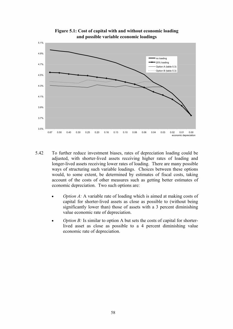
58

Figure 5.1: Cost of capital with and without economic loading and possible variable economic loadings

5.42 To further reduce investment biases, rates of depreciation loading could be

adjusted, with shorter-lived assets receiving higher rates of loading and longer-lived assets receiving lower rates of loading. There are many possible ways of structuring such variable loadings. Choices between these options would, to some extent, be determined by estimates of fiscal costs, taking account of the costs of other measures such as getting better estimates of economic depreciation. Two such options are:

• Option A: A variable rate of loading which is aimed at making costs of

capital for shorter-lived assets as close as possible to (without being significantly lower than) those of assets with a 3 percent diminishing value economic rate of depreciation.

• Option B: Is similar to option A but sets the costs of capital for shorter-lived asset as close as possible to a 4 percent diminishing value economic rate of depreciation.

3.5%

3.7%

3.9%

4.1%

4.3%

4.5%

4.7%

4.9%

5.1%

0.67 0.50 0.40 0.30 0.25 0.20 0.16 0.13 0.10 0.08 0.06 0.04 0.03 0.02 0.01 0.00

no loading 20% loading Option A (table 5.3) Option B (table 5.3)

economic depreciation

59

Table 5.3 Rates of economic loading under options A and B

Diminishing Value Rate

Economic Loading Option A

Economic Loading Option B

100% - -

67% 35% 30%

50% 35% 30%

40% 35% 30%

30% 35% 30%

25% 35% 25%

20% 30% 25%

16% 30% 25%

13% 30% 20%

10% 25% 20%

8% 25% 20%

6% 20% 10%

4% 10% -

3% - -

2% - -

1% - -

0% - -

5.43 The effects of these two options are shown in table 5.3.43 Under either

option no loading is calculated for two-year equipment which would qualify for a 100 percent depreciation deduction as it is not altogether clear how a loading could be applied to assets with a 100 percent diminishing value depreciation rate.44

5.44 Submissions are sought on whether there is merit in moving to a declining

economic loading as discussed here.

43 It is straightforward to extend to include other options, such as a higher cost option of provide a loading to keep costs of capital as close as possible to those of an asset with a 2 percent diminishing value rate of depreciation or a lower cost option of maintaining the 20 percent loading for shorter-lived assets and reducing the loading for longer-lived assets. 44 In principle, it would seem desirable to extend some tax benefit to these assets in lieu of a depreciation loading to maintain neutrality. One simple option might be to allow expensing for these assets.

60

Incorporation of assumption of inflation into tax rules 5.45 Relative to no loading or to a uniform 20 percent loading, these measures

appears to make investment decisions more neutral if inflation is within the Reserve Bank’s target range of 1 to 3 percent. These results also appear to be robust to reasonable alternative assumptions about the marginal rate of taxation.

5.46 An unattractive feature of the reforms is that they would be aimed at

offsetting a predicted average rate of future inflation. If inflation rates change in the future, the reforms could be much less attractive. Indeed, if inflation were eliminated, the reforms would end up introducing tax biases. However, the Reserve Bank currently has the mandate of keeping inflation in the 1 to 3 percent range and, at these rates of inflation, investment decisions would appear to be more neutral. Figure 5.2 shows costs of capital under inflation rates of 0, 1, 2 and 3 percent per annum.

5.47 Note it is not envisaged that loadings would be changed from year to year as

inflation rates change. To do so would be likely to be complex and add considerable uncertainty to the system. This means that some biases are likely to remain. There would be a case for reconsidering loadings, however, if it there were any change in the Reserve Bank’s target range for inflation.

Figure 5.2: Demonstration of impact of varied rates of inflation on option A

3.0%

3.5%

4.0%

4.5%

5.0%

5.5%

0.67 0.50 0.40 0.30 0.25 0.20 0.16 0.13 0.10 0.08 0.06 0.04 0.03 0.02 0.01 0.00

Ret

urn

zero

1%

2%

3%

Inflation rates

Economic depreciation rates

61

5.48 Figure 5.2 shows that for an inflation rate of 2 percent, the option A variable loading does a reasonable job in equalising rates of return on investment in assets with different depreciation rates. At an inflation rate of 3 percent, however, the variable loading is not as effective, reflected in the steeper rate of decline as asset lives increase. Correspondingly, if there were no inflation, the loading would clearly benefit short-lived assets over long-lived assets.

Other issues Asset depreciation bands 5.49 At present, there is a set of 14 depreciation bands. The number of bands

involves a compromise between simplicity and neutrality. A problem with depreciation bands is that close to a point of switching from one band to another there may be a significant bias between assets with very similar economic lives which fall into different bands. Increasing the number of depreciation bands reduces this problem but at the cost of greater complexity.

5.50 Submissions are sought on whether there should be more or fewer

depreciation bands. Second-hand assets, used imported motorcars and buildings (if relevant) bands 5.51 Currently, second-hand assets, used imported motorcars and buildings do not

qualify for any depreciation loading. 5.52 If the goal of depreciation provisions is to make investment decisions as

neutral as possible, it seems difficult to justify why there should be a lower rate of depreciation for second-hand than for new assets. In the absence of a loading for second-hand assets, there would appear to be an artificial tax bias discouraging firms from acquiring second-hand assets when these can be the most sensible assets to acquire. Thus there would appear to be a prima facie case for extending any loading to second-hand assets. Of course, providing loadings for second-hand assets would add to the fiscal cost of the loadings and, for a given revenue cost, reduce the loadings that could be paid.

5.53 Similar issues arise in the case of used imported motorcars. As depreciation

loadings are aimed at creating as neutral as possible an environment for investment, it is difficult to see why any particular assets should be excluded except if assets already benefit from concessional depreciation rates. Identical issues would arise in the case of buildings as well if they were estimated to depreciate sufficiently quickly to qualify for a loading.

5.54 Submissions are sought on whether there are any good policy reasons for

excluding second-hand assets, used imported motorcars or buildings (if relevant) from depreciation loadings.

62

Any other methods of better measuring economic depreciation 5.55 Submissions are sought on any other practical measures to better help

depreciation provisions to mirror economic depreciation. For example, we have discussed in chapter 4 the way in which two assets with the same economic life need not have the same profile of economic depreciation. A severe practical problem is that estimating an average economic life in order to provide a basis for calculating economic depreciation seems to be a difficult task in itself. Refining this measure for the way in which cash flows on individual assets decline seems impossible.

5.56 International studies suggest that allowing double declining balance may be a

more accurate way of measuring depreciation than, say, allowing straight-line depreciation for equipment. This is in large part because cash flows may decline rapidly for a number of reasons, including rapid technological improvement. Although recognising that this may accelerate depreciation deductions relative to economic depreciation for some assets and decelerate depreciation deductions for others, this may have to be accepted as one of the unavoidable difficulties of attempting to levy an income tax.

Submissions We invite submissions on these issues. In particular, we would like to receive submissions on: • introducing double declining balance depreciation for plant and equipment and

straight-line depreciation for buildings and other structures;

• the best ways of checking on the double declining balance approximation for shorter-lived plant and equipment;

• the best way of using New Zealand data to check the appropriateness of allowing straight-line depreciation or a diminishing value equivalent for buildings and other structures;

• how the suggested rules should address assets with substantial residual values;

• whether there are major generic problems with current estimates of economic lives;

• introducing an increased loading for shorter-lived assets matched with a lower loading on longer-lived assets;

• narrowing the depreciation rate bands into which assets are classified;

• extending the economic loading to second-hand goods, buildings and other structures and used imported motorcars; and

• any other method of calculating depreciation more accurately.

63

Part 3

Specific issues

This part of the issues paper considers more detailed aspects of the current rules and possible improvements to those rules. Issues are examined in the context of the current tax depreciation rules, including, for example, the way in which depreciation rates are set. Accordingly, the current rules relating to the assumed 13.5 percent residual value for economic depreciation rates may remove some of the difficulties discussed in this part. The issues considered in Part 3 are those that have been raised with officials by taxpayers or their representatives since the depreciation review was announced by the government, in early 2003. Part 3 also considers the tax treatment of rental housing. Chapters 6, 7 and 8 outline the various submissions received, our comments in relation to the concerns raised and, where applicable, suggested changes to the tax depreciation rules to address concerns and further improve the operability of the rules. It is our intention to report to the government on those measures we consider should be progressed (and are supported in feedback received on this issues paper) later this year. Chapter 9 considers various aspects of the tax treatment of rental housing including depreciation (in the context of breaking buildings into smaller depreciable assets). Chapter 10 outlines a number of depreciation issues that are being considered as part of other proposals.

65

Chapter 6

SUGGESTED TECHNICAL CHANGES TO THE TAX DEPRECIATION RULES

Summary • The rules in relation to claiming deductions for certain expenditure incurred in

preventing or combating pollution should be clarified by giving an amortisation deduction for these expenditures.

• A deduction should be allowed for site restoration expenditure in the year that

this expenditure is incurred, with businesses allowed to match the cost of site restoration against income previously generated from their business operations.

• When a patent is granted, any depreciation from the time that the patent is given

legal effect (when the complete application is lodged) up to the date of grant, should be allowed in the first income year in which depreciation can be claimed.

• Changes should be made to the special tax depreciation rate rules to: – relax the threshold on the Commissioner for considering special tax

depreciation rate applications by replacing the need for the Commissioner to be “absolutely” certain about the actual economic life of an asset with a requirement for the Commissioner to be only “reasonably” certain, before a special rate can be issued;

– clarify that the Commissioner may have regard to a broader range of factors than just the rate of depreciation adopted by the taxpayer for financial reporting purposes, when considering an application for a special tax depreciation rate;

– widen the Commissioner’s ability to prescribe special tax depreciation rates using a method other than the diminishing value formula in the legislation, if such a method is more appropriate;

– extend the six-month time bar on the Commissioner to consider special and provisional tax depreciation rate applications; and

– extend the special tax depreciation rules to apply to fixed-life intangible property, such as patents, if the Commissioner is satisfied that the actual economic life of the property will be less than its legal life.

• Plant variety rights (granted under the Plant Variety Rights Act 1987) should be

added to Schedule 17 of the Income Tax Act as depreciable intangible property (with the right to use plant variety rights also included in Schedule 17 as a clarification).

66

• The definition of “depreciable intangible property” should be clarified so that it is clear that property listed on Schedule 17 can be depreciated without having further regard to whether that property can, for example, be used for tax avoidance purposes.

• Deductions for losses on destruction of buildings as a result of natural disasters

(such as the February 2004 storms, earthquake and fire) should be allowed. The issue of losses on disposal of buildings more generally (including voluntary destruction) raises a number of avoidance concerns.

• It should be noted that a loss incurred on the destruction of a “temporary

building” is deductible for tax purposes and that the Income Tax Act 2004 clarifies this.

6.1 This chapter examines issues for which we consider change is feasible and

may be warranted (thereby providing useful technical improvements to the tax depreciation rules). Chapter 7 discusses issues about which we require further information before we can make recommendations. Chapter 8 analyses issues which we do not consider warrant changes to the rules.

6.2 Although we have tried to address a number of technical issues relating to the

tax depreciation rules, we recognise that the list of issues we have so far considered is not exhaustive. Consequently, we welcome submissions on other issues or problems that taxpayers face with the tax depreciation rules and any suggestions for improving them.

Expenditure incurred in preventing, combating or rectifying pollution 6.3 It has been submitted that a number of issues arise in relation to the ability to

claim deductions in respect of certain expenditure incurred in preventing, combating and rectifying pollution.

Background 6.4 Business taxpayers may claim a tax deduction for expenditure to prevent or

combat pollution of the environment in three ways:45

• under section BD 2 of the Income Tax Act 1994 for normal operating (revenue) expenditure;

• under the depreciation rules for certain types of capital expenditure, such as tanks, reservoirs, pipes, pumping machinery and screens; and

• under section DJ 10.

45 The review of environmental costs focuses on the treatment of these costs generally and does not consider industry-specific provisions (such as for the primary sector, mineral and petroleum mining).

67

6.5 Section DJ 10 allows business taxpayers to claim a deduction for the cost of

constructing on land in New Zealand any earthworks, ponds, settling tanks or other similar improvements primarily for the purpose of treating industrial waste in order to prevent or combat pollution of the environment.

6.6 If a deduction is available, it must be spread evenly over five years,

beginning with the year in which the expenditure was incurred (that is, a deduction for 20% in each year beginning with the year the expenditure was incurred), although amounts less than $1,000 can be deducted in full.

6.7 Section DJ 10 and its forerunners (section 124 of the Income Tax Act 1976

and section 113E of the Land and Income Tax Act 1954) were introduced by the Land and Income Tax Amendment Act (No.2) 1972 in response to a recommendation from the 1970 Physical Environmental Conference.

6.8 The speech notes and papers accompanying the Amendment Act indicate that

the section was introduced to permit business taxpayers a deduction for expenditure incurred for the purpose of treating industrial waste if no other allowance might otherwise be possible.

6.9 Despite the existence of a specific section to provide for deductions of this

nature, certain costs incurred in preventing or combating pollution are not currently deductible. There is uncertainty as to the scope of the tax deduction permitted, as the legislation refers to expenditure incurred primarily for the purpose of treating “industrial waste” (not defined). Furthermore, section DJ 10 allows a deduction only for capital expenditure incurred in constructing earthworks or similar improvements.

6.10 It appears that no deduction is available for dealing with non-industrial waste

or for expenditure which does not give rise to an identifiable land improvement. This is illogical and results in the incorrect calculation and taxation of income from business activities and has led to taxpayer submissions calling for a change to the legislation. We are therefore currently undertaking work on clarifying the scope of tax deductibility of expenditure to prevent or combat pollution of the environment.

6.11 A separate submission has also been received on the related issue of

restoration costs (reconstructing or returning a site to its original state). The tax treatment of restoration costs is also uncertain, which makes it difficult to correctly measure cessation costs. We are therefore also considering issues relating to the deductibility of costs incurred at cessation of business (such as those in relation to site restoration).

Comment Expenditure to prevent or combat pollution 6.12 To clarify the scope of deductions available for expenditure incurred to

prevent or combat pollution, we are considering revised tax rules for these costs.

68

6.13 Our preferred approach would be for pollution prevention assets to be

included within the depreciation rules in order to bring environmental expenditure in line with the treatment of capital expenditure generally. However, for a number of practical reasons,46 a depreciation approach is not feasible. Instead, officials are likely to recommend the following revised treatment of expenditure incurred to prevent or combat pollution:

• section BD 2 deduction for normal operating (revenue) expenditure;

• depreciation deduction for depreciable assets; and

• amortisation deduction under a revised section DJ 10 for other capital expenditure incurred in preventing or combating pollution, with no distinction made between treating industrial and other forms of waste. We will need to consider further the appropriate categories of expenditure and amortisation rates.

Restoration expenditure 6.14 As part of revising section DJ 10, a deduction would be allowed for capital

site restoration expenditure. This reflects the legal and moral obligations imposed on businesses to rectify pollution and ensures that business income is not overstated for tax purposes. However, even when site restoration expenditure is deductible (revenue deduction, depreciation or section DJ 10) this is of little use when incurred after a company has ceased business. At cessation of business, a taxpayer may incur expenditure related to deriving past income but have no current income against which to offset that expenditure.47 In such a situation, no benefit is obtained for the resulting loss, even though the taxpayer may have paid significant amounts of tax in the past. Under existing law, there is no ability to match this expenditure against income derived while carrying on the business.

6.15 Our view is that businesses should be allowed to match the costs of site

restoration against income generated from their past business operations, and we are considering what would be an appropriate mechanism for achieving this.

6.16 Matching income and deductions could be achieved by allowing a tax

deduction for accounting rehabilitation provisions. However, allowing a deduction for an estimate of restoration costs would be open to manipulation and would contradict the established taxation treatment of provisions for other costs.

46 For example, there are difficulties in classification, calculating estimated useful life and treatment on disposal. The amortisation provisions are driven off categories of expenditure, so asset classification is not an issue. There is also no claw-back or loss on disposal, so issues regarding valuation on disposal are avoided. 47 In relation to the closure of a business, there is an issue as to whether post-business cessation expenditure is necessarily incurred in the course of carrying on a business and, accordingly, whether that expenditure is deductible. The courts have considered this issue and established the general principle that expenditure incurred post-cessation will be deductible to the extent that the expenditure is sufficiently proximate to a company’s pre-cessation, ordinary business activity. Refer to the decisions in: Amalgamated Zinc (De Bavay’s Ltd) v FCT (1935) 54 CLR 295, AGC (Advances) Ltd v FCT 75 ATC 4057, FCT v Riverside Road Pty Ltd (In Liqtn) (1990) 23 FCR 305, Placer Pacific Management Pty Ltd v FCT 95 ATC 4,459, and C of T v Brown (1999) FCA 721. As part of resolving the matching issue for restoration costs, thought will be given to clarifying the tax deductibility of costs incurred on cessation which relate to prior business activity.

69

6.17 Jurisdictions such as the United Kingdom deal with this issue by allowing businesses to calculate a terminal loss on cessation of trade. The terminal loss may then be offset against earlier profits of that entity. The introduction of a loss carry back is not supported by officials because it is inconsistent with the general structure of New Zealand tax legislation and would create significant operational problems for both taxpayers and the Inland Revenue. For example, tax returns would have to be amended and reassessed. Instead, thought is being given to two other options which would provide a mechanism for matching expenditure incurred at cessation of business against income derived from business operations.

Establishment of a restoration fund48 6.18 Under this option, a taxpayer would be able to establish a restoration fund

with Inland Revenue. While the business is operating (and pollution resulting from its operations) a cash deposit could be made into the fund. This would be similar to establishing an accounting provision for site restoration but would give rise to a deduction for tax purposes equivalent to the gross amount of the deposit.49 Inland Revenue would enter the deposit into a restoration fund account with the Reserve Bank in the name of the taxpayer. At cessation of business, the taxpayer would request a refund from the restoration fund which would give rise to taxable income at the gross amount of the refund.50 However, any income would be offset by a tax deduction for restoration expenditure incurred by the taxpayer.

Formulaic loss offset

6.19 As an alternative to the restoration fund, we are also considering a proposal

to permit taxpayers to claim a refund for the lesser of:

• the tax effect of restoration costs incurred; and

• tax paid in a specified number of earlier periods. 6.20 The refund would relate to the year the restoration costs were incurred and,

as such, would not require re-filing and reassessment of earlier tax returns. 6.21 Each of these options has advantages and disadvantages. For example, the

restoration fund more accurately mirrors the accounting treatment, and allows matching over a longer period, while the formulaic loss rule gives a better result when there are unexpected levels of restoration costs.

48 A number of practical issues will need to be considered if either of the matching options is to be progressed further – such as links with restoration provisions maintained for accounting purposes, implications of a change in continuity, impact on taxpayers' imputation credit accounts and how and whether interest would apply. 49 For example, if the deposit is $33, the tax deduction would be $100. 50 For example, if the refund is $33, gross income for the taxpayer will be $100.

70

Suggested changes 6.22 We suggest that the rules in relation to claiming deductions for certain

expenditure incurred in preventing, combating and rectifying pollution be clarified by giving an amortisation deduction for capital expenditure incurred in preventing, combating or rectifying pollution. We also suggest allowing a deduction for site restoration expenditure in the year that this expenditure is incurred, with businesses allowed to match the cost of site restoration against income previously generated from their business operations.

6.23 This work is primarily being progressed by way of targeted consultation with

those directly affected by the narrow scope of section DJ 10 and those with significant site restoration costs. However, we would welcome submissions from other taxpayers on the proposed changes.

When depreciation can begin for patents 6.24 It has been submitted that patents should be depreciable from the time a

patent application is lodged, as the delay between lodging an application and the eventual grant of the patent can be several years.

Background 6.25 Under current tax law, depreciation deductions in respect of patents are

allowed from the date a patent is granted. Concerns have been raised that this “date of grant” approach has no regard to the date from which legal protection applies (the date when a complete patent application is lodged) or the time at which the underlying invention was used or was available for use.

6.26 It is worth noting, however, that the Commissioner of Inland Revenue

considers that the correct interpretation of the current rules is that the term of depreciation (legal life of twenty years) be reduced by the time taken for the patent to be granted (from lodgement date to grant date). This would result in higher depreciation deductions throughout the life of the patent (starting from the date of grant), than if full legal life was used.

Comment 6.27 In our view, the correct start date for depreciation in respect of a patent is

when it is granted, as this is when the asset (the legal protection over the rights to benefit from the underlying invention) comes into existence. Allowing patents to be depreciated starting from the time a patent application is lodged would effectively recognise the benefits conferred by a patent, for tax purposes, before the asset comes into existence. (For example, there is a risk that the patent may not be granted.)

71

6.28 The depreciation rules should, however, recognise that once a patent is granted, legal protection applies from the date a complete specification of the invention was lodged. Consequently, a portion of the depreciable life of a patent will have been expended in the period the patent is pending. Although, from a policy perspective, we consider that depreciation should start from the date a patent is granted, we recommend that the first depreciation deduction include any depreciation relating to the period from when the application was lodged to the time the patent is granted.

Suggested change 6.29 We suggest that when a patent is granted, taxpayers be able to claim any

depreciation from the time that the patent is given legal effect (that is, when the complete application is lodged) up to the date of grant, in the first income year in which depreciation is allowed.

When economic life is linked to an income-earning process or constrained by other factors (“tied assets”) 6.30 It has been submitted that when the economic life of an asset is inextricably

linked to the life of an income-earning process that is significantly shorter than the estimated useful life of the asset, for tax purposes, this should be better reflected in the tax depreciation rules.

Background 6.31 Concerns have been raised that when the usefulness of an asset is tied to an

income-earning process or business, the length of which is significantly shorter than the asset’s estimated useful life for tax purposes, application of the tax depreciation rules will result in an incorrect depreciation rate being applied. This is because the rate allowed will reflect a longer economic life than is actually the case. An example is plant and machinery employed in mining activities, when the estimated useful lives of these assets, for tax purposes, may be significantly higher than the duration of these activities (and when the activity is completed these assets, arguably, have no residual value).

6.32 These assets are typically referred to as “tied” assets. Typically, a deduction

for the remaining tax-book value will arise if a tied asset can no longer be used. However, this creates problems if, for example, there is insufficient income against which to apply the resulting deduction. Also, in respect of assets such as buildings, no loss on disposal will arise.

72

Comment 6.33 Taxpayers with so called tied assets can apply to Inland Revenue for a

special tax depreciation rate if the estimated useful life underlying the economic depreciation rate for an asset does not mirror its actual economic life. An instance where a special tax depreciation rate may be applicable is if a taxpayer will cease to be in business after a particular date, and the relevant asset cannot be salvaged for use by another taxpayer.

6.34 A key requirement when applying for a special tax depreciation rate is,

however, that taxpayers be able to provide sufficient information to the Commissioner in support of an application. This includes identifying the actual economic life of an asset with a very high degree of certainty. Although a depreciation rate for financial reporting purposing may assist in this, if the actual economic life of an asset cannot be clearly ascertained, a special tax depreciation rate will generally not be allowed. This has implications for tied assets employed in certain activities, such as mining, where the date of cessation of the activity is unlikely to be known with any great degree of certainty. Here, at any given time, only an estimation of (remaining) economic life can be made.

6.35 When taxpayers apply for a special tax depreciation rate, the requirement on

the Commissioner to have a very high degree of certainty in relation to when an asset will cease to be useful should be relaxed. For example, we are interested in exploring approaches that would lower the current threshold on the Commissioner to be “absolutely” certain about economic life when considering special tax depreciation rate applications. One option is to lower this threshold to require the Commissioner to be only “reasonably” certain about the actual economic life of a depreciable asset, before a special tax depreciation rate can be prescribed.

6.36 The difficulty that arises is defining what is “reasonably” certain. The

definition of “reasonably” certain could include, for example, an assessment of economic life based on data and other best estimates available at the time of a special tax depreciation rate application. In effect, a reasonableness test would take into account a range of factors such as the size of the business and the value of the asset. We would welcome feedback on the criteria that should be considered when considering the validity of a taxpayer’s special tax depreciation rate application.

6.37 A relaxation of the rules would, however, need to be supplemented by

measures to prevent taxpayers misusing special tax depreciation rates. Although a current provision, section EG 10(6) of the Income Tax Act, provides for revocation of special tax depreciation rate determinations, we consider these rules should be extended. Taxpayers would need to inform the Commissioner when the circumstances underlying a special tax depreciation rate have changed. Failure to notify the Commissioner or providing false information should result in application of penalties.

73

Suggested change 6.38 We are interested in options to relax the threshold on the Commissioner for

considering special tax depreciation rate applications – for example, replacing the need for the Commissioner to be “absolutely” certain about the actual economic life of an asset with a requirement for the assessment to be only “reasonably” certain, before a special rate can be issued. A lower threshold would need to be buttressed by rules to prevent misuse of the special tax depreciation rate mechanism.

The special tax depreciation rate rules 6.39 A number of technical problems also arise in relation to the special tax

depreciation rate rules, which can make it difficult for the Commissioner to make special tax depreciation rate determinations in certain circumstances. We consider that a number of improvements can be made to these rules.

Background 6.40 Section EG 10 of the Income Tax Act 1994 contains the rules in relation to

applications by taxpayers for special tax depreciation rates. The factors the Commissioner is required to have regard to include the legislative formula for calculating economic depreciation, and the rate of depreciation adopted for financial reporting purposes. The Commissioner can decline a special tax depreciation rate application if, generally:

• the rate calculated under the application would not differ significantly

from the general Commissioner-prescribed economic depreciation rate; or

• the general economic depreciation rate is already under review by the Commissioner and the new general economic rate will be equal to or greater than the rate calculated under the application; or

• insufficient information has been supplied to the Commissioner to calculate the appropriate rate.

6.41 A special tax depreciation rate issued by the Commissioner can be revoked if

the circumstances that applied at the time the determination was issued no longer exist or have materially changed.

Comment 6.42 The first issue is the requirement under section EG 10(2) of the Income Tax

Act for the Commissioner to have regard to the rate of depreciation (if any) adopted by a taxpayer for financial reporting purposes, along with the statutory depreciation rate formula (in section EG 4(3)). This creates difficulties if the rate adopted for financial reporting purposes is, for example, a straight-line rate, as the statutory depreciation formula is based on the diminishing value methodology. Consequently, when applying section EG 10(2) in respect of a special tax depreciation rate application, it is unclear

74

whether the Commissioner must have regard only to the rate used by the taxpayer, when it may also be appropriate to consider the taxpayer’s assessment of economic life, residual value and the method of depreciation.

6.43 We suggest that the special tax depreciation rate rules be clarified so that the

Commissioner is able to have regard to the taxpayer’s assessment of economic life, residual value and method of depreciation. Any clarification should include the ability to set a residual value of less than 13.5 percent (the current minimum in the legislative formula) if so warranted. A discussion on the relevance of (and problems with) the 13.5 percent residual value is provided in an earlier chapter.

6.44 Furthermore, the special tax depreciation rate provisions do not seem to

provide a clear legislative authority for taxpayers to be allowed depreciation methods other than diminishing value, for tax purposes. If a taxpayer applies to the Commissioner to adopt for tax purposes the straight-line depreciation rate that is used for financial reporting purposes, under the special tax depreciation rules that will generally not be allowed. This is because the straight-line depreciation rate used for financial reporting purposes is likely to be calculated in a different way from that calculated for tax purposes. For tax purposes, the rate is based on a diminishing value formula, with the aforementioned 13.5 percent residual value. An “equivalent” straight-line depreciation rate is then calculated. For accounting purposes, the straight-line depreciation rate may incorporate different parameters (for example, a 0 percent residual value), resulting in the financial reporting straight-line rate differing from that for tax purposes.

6.45 These problems become even more pronounced when the depreciation

method adopted for financial reporting purposes is neither diminishing value nor straight-line. An example is the “unit of production” depreciation methodology which determines depreciation based on the “…number of production or similar units expected to be obtained from the asset or the enterprise”.51

6.46 There is scope for looking at widening the powers of the Commissioner to

prescribe special tax depreciation rates that are not calculated having regard to the legislated diminishing value formula, if another depreciation method would provide a more economically correct result and can be applied with a “reasonable” degree of certainty.

6.47 Finally, a problem arises in relation to the six-month time limit that is

imposed on the Commissioner for issuing a special (or a provisional tax depreciation rate for that matter) under section EG 14(1). Under that provision, the Commissioner must either issue the rate sought or notify the taxpayer of the decision not to issue a determination within the specified period.

51 The decline in economic value is calculated per unit of use or production. The “unit of production” methodology has application in industries such as mining.

75

6.48 Owing to the potentially complex nature of some special and provisional tax depreciation rate determinations, however – such as the need to source accurate information about estimated useful lives and the time taken to consult with applicants on their applications – this six-month deadline can be breached. This can theoretically result in a special or provisional tax depreciation rate application being declined, not because the application is deficient but, rather, the time available to the Commissioner to consider it has expired. In practice, Inland Revenue attempts to consider special and provisional tax depreciation rate applications outside this period, if a taxpayer agrees to this. The issue that arises is whether determinations issued after the six-month time limit are supported in legislation.

6.49 We consider that the law should be clarified and greater flexibility should be

allowed to the Commissioner to consider special and provisional tax depreciation rates outside the six-month time bar, if it is apparent that the deadline will be breached and the applicant agrees to such an extension.

Suggested changes 6.50 We suggest changes to the special tax depreciation rate rules to clarify that

the Commissioner may have regard to a broader range of factors than just the rate of depreciation adopted by the taxpayer for financial reporting purposes, when considering an application for a special tax depreciation rate. We also suggest that consideration be given to widening the Commissioner’s power to prescribe special tax depreciation rates using a method other than the legislated diminishing value formula, if such a method is more appropriate. Consideration should also be given to extending the six-month time bar on the Commissioner to consider special and provisional tax depreciation rate applications.

Economic life of patents and other fixed-life intangible property 6.51 It has been submitted that the twenty-year depreciation period for patents has

no regard to real economic life, which is effectively the commercial life of the underlying invention (including the technological obsolescence of the invention) and the period within which competitors can develop alternatives to work around the patent. Submissions have commented that patents should be allowed to be depreciated over the economic life of the underlying invention, not the legal life of the patent.

Background 6.52 Although patents have a maximum legal life of twenty years, they must be

renewed at the end of the fourth, seventh, tenth and thirteenth years for legal protection to be ongoing. A taxpayer can choose, by not renewing a patent, to cease use of the patent. For tax purposes, a deemed disposal will typically arise, allowing any non-depreciated capitalised costs then to be written off.

76

Comment 6.53 Although taxpayers may cease use of a patent before the cessation of its

potential legal life, the length of time over which legal protection is available is the most easily accessible proxy for the economic life of patents (and most other types of depreciable intangible property). This is because the actual economic lives of most intangible property are often quite difficult to ascertain with any degree of certainty. If taxpayers were to use the commercial life of the underlying invention – for example, as a proxy for the economic life of a patent, significant verification issues would arise.

6.54 It may be possible, however, to extend the use of the special tax depreciation

rate rules to patents, and other fixed-life intangible property, if a taxpayer can show that the economic life of the patent (or the other property) will be less than its legal life. This would enable taxpayers to depreciate fixed-life intangible property over a period which more closely reflects the true economic life of that property, if the Commissioner is satisfied that economic life is sufficiently different to legal life.

6.55 At present, section EG 10(1) of the Income Tax Act prohibits the

Commissioner from prescribing a special tax depreciation rate in respect of fixed life intangible property. This approach has been due to concerns about the ability to abuse the tax depreciation rules in respect of assets that cannot easily be valued. We consider that these concerns are largely still valid. Consequently, any extension of the special tax depreciation rules in respect of patents and other fixed-life intangible property would require the Commissioner to be satisfied, with a high degree of certainty, that the actual economic lives of the property in question were sufficiently different from their legal lives. Owing to the nature of the property involved, we do not think it is unreasonable for the Commissioner to meet a “high” certainty threshold before a special tax depreciation rate is allowed (rather than the suggested “reasonable” certainty threshold in the case of depreciable property such as plant and machinery). This could include, for example, requiring taxpayers to explicitly link, say, a patent to the economic life of the underlying invention or process. We are interested in submissions on how this could be achieved.

6.56 We have also considered whether it is possible to allow specific tax

depreciation rules for patents (and other fixed-life intangible property), similar to those allowed for the copyright in a sound recording. A copyright in a sound recording can be depreciated from the time it might reasonably be expected to be first useful in deriving gross income to the year in which it is reasonably expected that 90 percent of all the income from the copyright will be derived – calculated at one year. This depreciation treatment was determined after extensive consultation with valuers and asset owners, and it may be possible to do a similar quantitative exercise in relation to other fixed-life intangible property. The concern we have with using this type of method to prescribe a general depreciation rate in respect of, for example, patents (other than the scope and cost of such an exercise) is that such an analysis may not necessarily result in an accurate measure of economic life because the results may vary significantly, depending on the type of patent

77

(which will depend on the underlying invention). Consequently, we do not prefer such an option.

Suggested change 6.57 We suggest that consideration be given to extending the special tax

depreciation rules to apply to fixed-life intangible property, including patents, if the Commissioner is satisfied that the actual economic life of the property will be less than its legal life.

Plant variety rights included as depreciable intangible property 6.58 It has been submitted that plant variety rights should be added to the list of

depreciable intangible property (in Schedule 17 of the Income Tax Act), with the property being depreciable over the commercial life of the underlying plant variety.

Background 6.59 A grant of plant variety rights under the Plant Variety Rights Act 1987 gives

the holder the exclusive right to produce for sale and to sell propagating material of the plant variety for a period of twenty or twenty-three years (depending on the plant material).

Comment 6.60 The criteria for inclusion as depreciable intangible property includes having

“…a finite useful life that can be estimated with a reasonable degree of certainty on the date of its creation or acquisition” and “if made depreciable, a low risk of being used in tax avoidance schemes”.52 We consider that plant variety rights meet these criteria, as useful life can be equated with legal life – a period of approximately twenty or twenty-three years – and the process that must be followed for a grant of plant variety rights is reasonably robust (set in statute). Plant variety rights should therefore be added to Schedule 17 of the Income Tax Act.

6.61 Although it has been submitted that plant variety rights should be depreciable

over the commercial life of the underlying plant variety, it would be difficult to align useful life for tax purposes with the commercial viability of a plant variety (for the same reasons that it is difficult to do so in the case of a patent, which is very similar in nature to plant variety rights). Consequently, as a starting point, we consider plant variety rights should be depreciated over their legal life – twenty or twenty-three years, depending on the plant variety – on a straight-line basis. This is consistent with the treatment of fixed-life intangible property (including patents). However, if included as depreciable intangible property in Schedule 17 of the Income Tax Act, the suggested change to extend the special tax depreciation rate rules to fixed-life intangible property should apply equally in the case of plant variety rights.

52 Refer definition of “depreciable intangible property” in section OB 1 of the Income Tax Act 1994.

78

6.62 In terms of expenditure that should be capitalised and depreciated, we consider that costs incurred in registering plant variety rights, acquiring outright interests in plant variety rights, licensing the right to use plant variety rights, and protecting or enhancing plant variety rights would qualify. We note, however, that this is not an exhaustive list and, therefore, we would like further information on the types of expenditure that may be associated with plant variety rights applications and, where possible, the likely quantum of such expenditure.

6.63 As a further clarification, we consider that the right to use plant variety rights

should also be added to the list of depreciable intangible property in Schedule 17.

Suggested changes 6.64 We suggest that plant variety rights (granted under the Plant Variety Rights

Act 1987) be added to Schedule 17 of the Income Tax Act as depreciable intangible property, with depreciation over legal life. As a further clarification, the right to use plant variety rights should also be included in Schedule 17.

Clarifying the definition of “depreciable intangible property” 6.65 We consider that the definition of “depreciable intangible property” should

be clarified. Background 6.66 Section EG 1 of the Income Tax Act allows a deduction in an income year

for an amount on account of depreciation for any depreciable property owned by a taxpayer in an income year. Depreciable property does not include intangible property unless that property is depreciable intangible property. Section OB 1 defines depreciable intangible property to be:

“…property of a type listed in schedule 17, which schedule describes intangible property that has- (a) A finite useful life that can be estimated with a reasonable degree of certainty on the date of its creation or acquisition; and (b) If made depreciable, a low risk of being used in tax avoidance schemes:”

79

Comment 6.67 The issue that arises is in relation to the definition of depreciable intangible

property (above), and the wording following the reference to Schedule 17 of the Income Tax Act [in italics]. It is unclear whether the wording is a preamble to Schedule 17 or has legislative force – that is, whether in addition to being an intangible asset listed on Schedule 17, it must have a finite useful life, and more importantly, a low risk of being used for tax avoidance purposes, before depreciation can be claimed.

6.68 A clarification is necessary to ensure that the relevant wording is interpreted

simply as an introduction to Schedule 17 – that is, a description of the characteristics of the property included in Schedule 17 – and therefore carries no legislative weight.53 This is because the policy intention is for Schedule 17 to list exhaustively the types of intangible property that are depreciable and if listed, such property should be depreciable, without further consideration being having to be paid to whether, for example, the property can be used for tax avoidance purposes.

Suggested change 6.69 We suggest that the definition of “depreciable intangible property” be

clarified so that it is clear that property listed on Schedule 17 can be depreciated without having further regard to paragraphs (a) and (b) of the definition.

Deductibility of losses on disposal of buildings and other structures 6.70 There is merit in looking at allowing a deduction for losses on disposition of

buildings. Background 6.71 Under section EG 19(3) of the Income Tax Act, deductions for losses on

disposal of buildings are not allowed. Similarly, section EG 12(1) does not allow a deduction for the remaining tax-book value of a building, if the building is no longer used (and the cost of disposition would exceed any consideration derived). The government is, however, considering whether losses in relation to buildings used to derive gross income that are damaged in natural disasters should be deductible, in response to the damage caused by the storms in February of this year.

53 There would be significant compliance costs associated with the use of Schedule 17 if taxpayers were required to come to a conclusion on whether depreciable intangible property listed on it also met paragraphs (a) and (b) of the definition.

80

Comment 6.72 At first glance, there would seem to be an asymmetry in the current

depreciation rules for buildings. When buildings are sold for more than their written-down tax-book value (as for other assets) excess depreciation is clawed back on sale. However, differently from other assets, if buildings are sold or otherwise disposed of for less than their written-down tax-book value, the loss is not deductible.

6.73 In 1992 the Consultative Committee on the Taxation of Income from Capital

(the Valabh Committee) reviewed the depreciation treatment to be applied to business assets. It concluded that it could see no justification for discriminatory treatment between different types of depreciable property, and that all depreciable property should be treated in an identical manner on disposal. It recommended that losses on disposal of buildings should be deductible in the same way as losses on disposal of other assets, a recommendation not supported by the government at that time.

6.74 We agree that there is a prima facie case for allowing a general deduction for

losses on disposition of assets. However, there is an important balancing consideration. If buildings are sold for more than their original purchase price, while depreciation is clawed back (so the difference between the acquisition cost and the written-down tax-book value is taxed), no tax is normally levied on the difference between the disposition proceeds and the acquisition cost (because New Zealand does not have a general capital gains tax). Although buildings may normally be expected to depreciate over time, rates of depreciation are typically low. On the other hand, the value of land improvements (including buildings) is normally calculated as the difference between the overall value of a property and unimproved value of the land. As the overall value of a property and the unimproved value of land are both subject to fluctuations, the value of improvements can be quite variable. If gains are not taxed when buildings appreciate, there is an argument for not allowing deductions for losses on sale. Although similar issues can arise for other assets, this is likely to be a particularly important problem for buildings because of their low depreciation rates and the way that the value of improvements is calculated.

6.75 This issue is different, however, in the case of buildings that are destroyed.

In principle, there would be strong grounds for a general deduction for losses when buildings are destroyed. Buildings can be destroyed either voluntarily (for example, to build a superior building) or involuntarily because of catastrophic events (such as the recent floods). In the case of voluntary demolition, there is, however, a potential concern. It is often difficult to be certain exactly how much of the acquisition cost of a property is attributable to the building and how much is attributable to the land. If losses for voluntary destruction were deductible, there would appear to be scope for taxpayers to acquire buildings shortly before they were due to be destroyed in order to obtain a tax deduction on disposal. Taxpayers might also be able to attribute a substantial proportion of the value of the property to the buildings to create an artificial loss, which might be difficult to police.

81

6.76 Neither of these issues appears relevant, however, in the case of properties that are destroyed because of natural disasters (such as floods, earthquakes and bushfires). This is because the scope to manipulate the rules is unlikely to be significant in such circumstances.

6.77 The list of circumstances could also be widened to include losses arising

from the requirement to destroy a building by a local or a public authority (such as the reclamation of land for public works purposes – such as the construction of new roads).

6.78 In the case of losses on voluntary destruction of buildings, the greatest scope

for manipulation appears to arise when an asset outside the tax base is sold to a business shortly prior to its destruction.

6.79 A solution may be to limit losses more generally to buildings that have

predominantly been inside the tax base – such as buildings used in a taxpayer’s income-earning process. There are, however, a number of problems with this, particularly in relation to asset definition – for example, the boundary between “business” and “non-business” buildings is difficult to define and enforce. We invite submissions on how such a boundary could be defined and maintained.

6.80 Limiting deductibility to losses on destruction of buildings also creates a

tension in relation to other forms of “disposal”, namely the sale of buildings for consideration below their tax-book value. If losses on voluntary destruction of buildings are allowed but losses on sale are not, this could result in a “lock-in” effect in favour of a particular type of disposition, which would be inefficient. Consideration, therefore, needs to be given to the issue of the wider tax treatment of losses on disposal of buildings. However, the tax avoidance concerns that arise in relation to allowing losses on voluntary destruction of buildings would arise equally (if not more so) if losses on sale of buildings were allowed. These concerns would have to be balanced against the potential improvements to the efficiency of the tax depreciation rules. We have identified no solution which we consider achieves our efficiency goals at acceptable revenue risk.

6.81 Any change to extend deductibility on destruction of disposal of buildings

could also extend to involuntary destruction of farming land improvements. Suggested change 6.82 Although we consider that deductions for losses on destruction of buildings

should be allowed if the destruction is involuntary (e.g. the result of a natural disaster), the issue of allowing deductibility for losses on voluntary destruction of buildings and losses on disposal more generally (for example, on sale) is more difficult as there is substantial scope for manipulation of the rules. We invite submissions on potential solutions.

82

Deductibility of losses on disposal of temporary buildings 6.83 It has been submitted that clarification is needed that a loss on the disposal of

a “temporary building” is deductible for tax purposes. Background 6.84 A “temporary building” is defined in section OB 1 of the Income Tax Act as

any building which has been erected:

• under a permit issued by a local or public authority which is subject to demolition or removal on instruction by a local or public authority; or

• at a construction site and is to be demolished or removed on or before completion of the construction; or

• which was erected and is used for the purpose of housing plant or machinery and would have to be demolished in removing or replacing the machinery.

6.85 Section EG 19(3) states that when depreciable property is disposed of by a

taxpayer for a consideration that is less than its depreciated value (for tax purposes), the difference is allowed as a deduction to the taxpayer. The exception to this rule is if the depreciable property is a building. On the other hand, section DD 1(1)(c) states that no deduction is allowed for any loss incurred on the demolition or destruction of any premises, other than a temporary building.

Comment 6.86 The policy intention is for losses on the disposal of a “temporary building” to

be deductible, if the building is destroyed. This has been clarified in the re-written Income Tax Act 2004, in section DB 14 of that Act, which states that:

“A person is allowed a deduction for a loss that they incur through the destruction of a temporary building.”

6.87 The Income Tax Act 2004 applies from the 2005-06 income year and,

consequently, we do not consider an urgent change to existing legislation is necessary.

Suggested change 6.88 It should be noted that a loss incurred on the destruction of a “temporary

building” is deductible for tax purposes and that the Income Tax Act 2004 clarifies this point.

83

Chapter 7

ISSUES ABOUT WHICH MORE INFORMATION IS NEEDED

Summary • Although in principle, asset disposal costs should be fully deductible, greater

information is required on what these costs are and in what circumstances they may arise, to assist in more fully considering the implications of such a change.

• A higher threshold ($2,000) for immediately deducting the cost of “low-value”

and a higher total threshold ($20,000) for immediately deducting the cost of “low-value” assets purchased at the same time from the same supplier does not seem justified as the fiscal cost is likely to exceed any compliance cost savings. To be able to deal with the matter, however, we request further information on this issue, including the write-off thresholds adopted for financial reporting purposes.

Deductibility of asset disposal costs 7.1 It has been submitted that when a depreciable asset is disposed of and the

consideration derived is less than the costs incurred in disposing of the asset, any excess expenditure should be deductible for tax purposes.

Background 7.2 A deduction for asset disposal costs is allowed under the definition of

“consideration” in section EG 19(10) of the Income Tax Act. Under paragraph (b) of that definition, the amount of any consideration derived is reduced by the amount of any asset disposal costs. This effectively means that a deduction for disposal costs is allowed to the extent these costs reduce consideration, and this reduction gives rise to a loss on disposal (under section EG 19(3)).54

7.3 What is unclear is whether asset disposal costs in excess of the consideration

derived (thereby resulting in a negative figure for consideration) are allowed as a deduction – that is, whether the legislation supports the concept of “negative consideration”. Under this concept if, for example, no net consideration is derived on the disposal of an asset because significant disposal costs are incurred, a loss on disposal (amounting to the remaining tax-book value of the asset plus any excess disposal costs) would nevertheless arise.55

54 Or a reduction in any claw-back of depreciation (under section EG 19(2)). 55 For example, an asset has been depreciated to a tax-book value of $30,000. The asset is disposed of for a (gross) consideration of $20,000, but the cost of disposing of the asset is $25,000. Under section EG 19(10), it is unclear whether a deduction is allowed for $30,000 (the disposal costs reducing consideration to $0, hence a loss on disposal of $30,000) or $35,000 (the disposal costs resulting in “negative consideration” of $5,000 and consequently a loss on disposal of $35,000).

84

Comment 7.4 The potential non-deductibility of certain asset disposal costs can result in

harsh outcomes when significant disposal costs arise in respect of depreciable assets. In some cases disposal in a particular manner is a prescribed condition of the right to use or right to construct a particular asset – for example, if the use and subsequent disposal of an asset has implications under the Resource Management Act 1991. Here, taxpayers may effectively be “locked into” incurring these costs. We therefore agree in principle that these costs should be deductible in full.

7.5 To assist us, however, in fully considering the implications of allowing full

deductibility for asset disposal costs (including the fiscal cost) we would like further information on these costs, including specific examples, and the instances in which they may arise.

Process for further consideration 7.6 We request further information on asset disposal costs, including what these

costs are and in what circumstances they may arise, to help us to consider this issue more fully.

Higher threshold for immediately deducting the cost of “low-value” assets 7.7 It has been submitted that the thresholds for immediately deducting the cost

of “low-value” assets should be raised, from the current level of $200 to $2,000, with a total threshold of $20,000 for immediately deducting the cost of “low-value” assets purchased at the same time from the same supplier (currently $200 as well).

Background 7.8 Under section EG 16 of the Income Tax Act 1994, the cost of assets acquired

for $200 or less can be immediately deducted, provided principally that the assets are not purchased from the same supplier at the same time as other assets to which the same depreciation rate applies (unless the total cost is $200 or less). The thresholds are there to minimise the compliance costs associated with depreciating large numbers of “low-value” assets when there is little gain in accuracy in income measurement between depreciation and expensing.

Comment 7.9 The issue of raising the “low-value” asset thresholds was considered by the

Committee of Experts on Tax Compliance in 1998. The committee concluded that although the benefit of raising the threshold for immediately expensing “low-value” assets would be a reduction in compliance costs, it had to be weighed against other factors, including the resulting economic distortions and the fiscal implications for government. In relation to the former, the committee recognised that raising the threshold would accelerate

85

deductions for a bigger set of assets, relative to those assets for which immediate deductibility was not allowed. More importantly, it considered that the revenue costs of such a measure, although transitional, would be significant, especially upfront.56 Further, an increase in the “low-value” asset threshold could increase the possibility that the rules could be abused. Finally, the committee considered that the pool method of depreciation could be used for assets valued between $200 and $2,000, thereby resulting in simpler depreciation rules. For these reasons, and because “…taking into account the revenue cost, it was not clear that the compliance cost savings would be equally significant”, the committee did not recommend increasing the $200 threshold for immediately expensing “low-value” assets.

7.10 In relation to assets purchased at the same time from the same supplier, the

committee considered that the $200 threshold imposed compliance costs that were out of proportion to the cost of items purchased by taxpayers. For example, if items valued below the $200 individual “low-asset” threshold are bought in bulk from the same supplier, the resulting purchase is required to be capitalised and depreciated. However, if the items are purchased not in bulk but in a number of separate transactions, each item is immediately deductible. This imposes compliance costs because taxpayers have to make related purchases of property under $200 in value in multiple transactions (or over multiple days) to avoid the application of the depreciation rules. Therefore the committee recommended raising the threshold (to $500) subject to the reduction in compliance costs mirroring the revenue cost. The committee did not consider that the revenue cost of raising the threshold for immediately expensing items bought from the same supplier at the same time could be accurately quantified without a wide-ranging survey of taxpayers and purchased assets. However, if the revenue cost for increasing to $500 the $200 “low-value” asset threshold is indicative (see footnote), the cost of any change in this area is unlikely to be insignificant. Consequently, we consider it unlikely that the revenue costs of such a change would be offset by the compliance cost benefits. Even so, we invite further submissions on this issue, particularly in relation to the thresholds adopted by taxpayers for immediately expensing the cost of assets for financial reporting purposes. Other information that would be useful includes information on the types of assets likely to be purchased by taxpayers at the same time and from the same supplier, the costs involved, and the compliance benefits from expensing versus, say, using the pool method of depreciation.

Process for further consideration 7.11 Although we do not suggest a change to the thresholds for immediately

deducting the cost of “low-value” assets, owing to the potential revenue costs involved, we invite further submissions on this issue.

56 Advice provided by officials, at the time, on a $500 threshold for “low-value” assets suggested a revenue cost of $115 million in the first year of such a change, $405 million in the second year, and $117 million in the third year.

86

Chapter 8

CHANGES WE DO NOT AGREE WITH

Summary • Taxpayers should not be allowed to use depreciation rates used for financial

reporting purposes for tax purposes. The Commissioner is already required to have regard to depreciation rates used by taxpayers for financial reporting purposes, both when setting general economic depreciation rates and special tax depreciation rates.

• The requirement that land held by a dealer in land be treated as being held on

revenue account for a period of ten years from the date of acquisition should not be amended to allow depreciation on buildings and other fixtures constructed on the land. We do not consider that workable rules to achieve this can be devised without providing significant scope for manipulation of those rules, although we invite feedback on this issue and any solutions that may be workable.

• No clarification is required in respect of the rules governing depreciation

previously allowed in relation to depreciable assets that change over to being held on revenue account. The tax depreciation rules trigger a deemed disposal at market value.

• No clarification is necessary in relation to the process for selecting a tax

depreciation rate that most reasonably reflects an asset’s economic life, as the current tax depreciation rules already provide a number of steps for selecting the most appropriate depreciation rate in respect of an asset, having regard to factors such as use in different industries.

• There is no material difference between the “economic life” of an asset and its

“estimated useful life”, for tax purposes, as the latter requires the Commissioner to take into account the factors that are relevant in the calculation of economic life. Therefore no change is recommended.

Use of financial reporting depreciation rates for tax purposes 8.1 It has been submitted that greater reliance should be placed on allowing

taxpayers to use financial reporting depreciation policy for tax purposes, if it is appropriate. For example, estimated useful life adopted for accounting purposes, when it conforms to financial reporting standards and law (such as Generally Acceptable Accounting Principles, or GAAP) and is applied consistently from year to year, with specific anti-avoidance measures to bolster this approach, if necessary.

87

Background 8.2 The Commissioner of Inland Revenue, when determining economic

depreciation rates for different assets, is required to consider rates adopted in respect of those assets, for financial reporting depreciation purposes. Administratively, economic depreciation rates are typically set by the Commissioner after consultation with affected taxpayers and independent valuers. This is designed to ensure that the resulting economic depreciation rate for an asset is at least broadly comparable to financial reporting depreciation rates.

8.3 There are, however, certain material differences in the way economic

depreciation rates are calculated by Inland Revenue, namely the use of a 13.5 percent residual value. Consequently, depreciation rates for tax purposes are unlikely to perfectly match accounting depreciation rates. The validity of the 13.5 percent residual value assumption and alternative economic depreciation methodologies are discussed in earlier chapters.

Comment 8.4 Our concern about allowing blanket alignment of tax depreciation rates with

financial reporting depreciation rates is the potential for accounting policy to drive tax outcomes. This raises issues in relation to the accounting treatments that are acceptable and the treatment of taxpayers who are not required to follow prescribed financial reporting standards. Although taxpayers applying financial standards, such as GAAP, are required to have regard to the substance of transactions rather than the form, if there is no requirement (or incentive) to comply there may be opportunities to use accounting policies for tax avoidance purposes. This is particularly a concern in relation to many small taxpayers as they will not be subject to financial reporting standards. Consequently, there is a risk that they may overestimate the depreciation rate on assets, as there will be no constraints against them doing so. Although it may be possible, as suggested, to design specific anti-avoidance rules to mitigate such activity, this would simply add complexity to the rules.

8.5 More importantly, we consider that the current tax depreciation rules have

appropriate mechanisms to deal with instances where taxpayers have concerns with depreciation rates prescribed by the Commissioner being significantly different to those used for accounting purposes. As noted earlier, if a depreciation rate thus prescribed does not accurately reflect actual economic life, taxpayers can apply for a special tax depreciation rate. The special tax depreciation rules in section EG 10(2) of the Income Tax Act require the Commissioner to have regard to the depreciation rate used for financial reporting purposes. The suggested changes to broaden the factors that the Commissioner must have regard to when considering an application for a special tax depreciation rate should further increase the incidence of tax depreciation rates not being significantly divergent from the accounting treatment. The suggested changes to broaden the applicability of special tax depreciation rates should also encourage greater use of these rules if there are

88

genuine discrepancies between, for example, actual economic life and estimated useful life for tax purposes.

Conclusion 8.6 We suggest that there be no change to the Commissioner’s prescription of

general economic depreciation rates. The Commissioner is required to consider depreciation rates used by taxpayers for financial reporting purposes, both when setting general economic depreciation rates and special tax depreciation rates. The latter provides a robust mechanism for taxpayers to challenge depreciation rates prescribed by Inland Revenue. The proposals discussed earlier to provide greater flexibility in the application of the special tax depreciation rules should also improve the overall operability of the tax depreciation rules.

Depreciation of buildings (and other fixtures) on land held by a dealer in land 8.7 It has been submitted that when land is not acquired with the purpose or

intention of resale, depreciable assets constructed on the land should be depreciable from the day the assets are available for use. If a taxpayer is a dealer in land (for example, a property developer) any land acquired is generally deemed to be held on revenue account for a period of ten years, even if acquired with no purpose or intention of resale. It has been submitted that buildings and fixtures constructed on the land cannot, therefore, be depreciated until this period has lapsed.

Background 8.8 Section CD 1(2)(b) of the Income Tax Act 1994 treats as gross income any

amount derived from the sale of land if a taxpayer is in the business of dealing in land and the land is sold or disposed of by the taxpayer within ten years after the date on which the taxpayer acquired it.

8.9 Section CD 1(3) provides an exemption from section CD 1(2)(b) to the

extent that the land comprises “… premises acquired and occupied by a taxpayer primarily and principally as premises from which substantial business is carried on by the taxpayer” or is used by the taxpayer “…primarily and principally as a residence” (subject to certain other conditions).

Comment 8.10 When land and buildings are being used as premises for carrying on a

business, even if a taxpayer is a dealer in land, the land is generally not treated as being held on revenue account. Consequently, depreciation can be claimed in respect of buildings and other fixtures constructed on the land.

89

8.11 When land (caught by section CD 1(2)(b)) is not acquired for the purposes listed in section CD 1(3), any buildings or other fixtures constructed on the land will arguably not be depreciable. This is because the land (inclusive of the buildings and fixtures) will be revenue account property,57 and proceeds from the sale of revenue account property are gross income, for tax purposes, with a deduction allowed for the cost of the property. Here, cost would include the cost of constructing the buildings and fixtures and is allowed as a deduction under section BD 2(1)(b)(i) or (ii) of the Income Tax Act. Paragraph (b)(vi) of the definition of “depreciable property” in section OB 1 of the Income Tax Act specifically excludes property whose cost is allowed as a deduction under section BD 2(1)(b)(i) or (ii).

8.12 We have considered whether the correct treatment for revenue account

property is for such property to be depreciable. Arguably, no depreciation deduction should be allowed in relation to revenue account property that is acquired and held solely for resale. This is because a deduction for the cost of the property will be allocated to the year of sale under section EF 2 of the Income Tax Act and, therefore, allowing depreciation would result in a mismatch with income derived from the sale of the property.

8.13 There may be instances, however, when an asset may be owned by a

taxpayer who is subject to tax on its sale because the selling of the property is an integral part of their business, but the property is used until sale to produce income – that is, buildings subject to section CD 1(2)(b). For example, if a building is revenue account property under section CD 1(2)(b)(ii) but is used as a rental property, arguably, a deduction for depreciation should be allowed. This is because the asset will result in income from two sources: income derived on sale and the rental activity. The matching concept would indicate that some part of the expenditure on the asset should be allowed against the income earned from the property while it is held.

8.14 An option is to allow depreciation in respect of an asset if it is revenue

account property as defined in the Income Tax Act and is used or available for use in deriving gross income other than the proceeds of sale with a deduction for the cost of the asset58 deferred until the asset is disposed of. However, we have concerns about applying such a solution to buildings when the owner is a dealer in land.

57 “Revenue account property” is defined in section OB 1 as “…property which is trading stock of the person or otherwise property in respect of which any amount derived on disposition would be gross income”. 58 Reduced for any depreciation allowed.

90

8.15 The ten-year rule in section CD 1(2)(b)(ii) is designed to remove the uncertainty and the risks associated with determining intention in relation to transactions involving land when one of the parties to the transaction is a dealer in land. We are not confident that the option above would be effective in differentiating between land purchased for resale and land purchased for other purposes, without creating significant opportunities for tax avoidance. By extension, we are not confident that a workable rule could be designed to allow depreciation in respect of buildings and fixtures on land not held for resale without providing opportunities for taxpayers to abuse the rule in respect of assets constructed on land that is held for resale. Even so, we invite feedback on this issue and the form of any other such solutions and how they would deal with tax avoidance concerns.

Conclusion 8.16 We do not consider that the current requirement that any land held by a

dealer in land be treated as being held on revenue account for a period of ten years from the date of acquisition should be amended. We invite feedback, however, on this issue and any workable solutions that would address our principal concern.

Treatment of property that changes use 8.17 It has also been submitted that when buildings move from capital account to

revenue account, as a consequence of, for example, land subdivisions and the buildings have been depreciated before the move, the treatment of the depreciation correctly claimed by the taxpayer before the transfer is uncertain.

Background and comment 8.18 Under section EG 19, a deemed disposal arises when any depreciable

property changes use in a year,59 including moving between capital and revenue account. Section EG 19(7) treats the property as having been disposed of for a consideration equal to its market value if the disposal is triggered by a change in use. Consequently, depending on whether market value is less than (or greater than) the tax-book value, a loss on disposal (or a claw-back of depreciation allowed) will arise. In the case of buildings, although depreciation may be clawed back, no loss on disposal will arise.

Conclusion 8.19 We do not consider that a clarification is required as the depreciation rules

trigger a deemed disposal at market value when property moves between capital and revenue account.

59 See paragraph (a)(iii) of the definition of “disposal” in section EG 19(9).

91

Depreciation rates under the industry and asset categories 8.20 It has been submitted that it is not clear whether taxpayers are intended to

have a choice between default depreciation rates in the asset and industry categories if particular assets are not specifically provided for in either, yet broadly fit within both. It has been submitted that the depreciation rules should be clarified to confirm that taxpayers are able to choose the depreciation rate that most reasonably reflects economic life.

Background 8.21 The asset and industry categories were introduced as part of the 1993 review

of the tax depreciation rules – as determination DEP 1. The steps shown in figure 8.1 should be followed to find the most suitable depreciation rate in respect of an asset.

Figure 8.1: Process for finding the most suitable depreciation rate

* Not the default rate for the industry or asset category

Industry category available

Rate available for asset*

Use rate

Asset category available

Rate available for asset*

Use rate

Asset listed in alphabetical listing

Use rate - if multiple listings use rate for closest industry

Asset category available

Industry category available

Apply for provisional rate

Use default rate for relevant asset class

Use default rate for relevant industry

No

No

No

No

No

YesYes

Yes Yes

Yes

Yes

Yes

No

No

92

8.22 Depreciation rates for assets under the industry category are determined having regard to industry-specific use and, consequently, should generally be used only by taxpayers in the relevant industry.60 When an asset is used in more than one industry, and not all the relevant industries are represented in the industry category, a general depreciation rate for the asset is also determined under the asset category. Depreciation rates under the asset category are set having regard to the potentially different uses of an asset in different industries.

8.23 The default rates under the asset and industry categories are an average of all

assets in the relevant asset class (in the case of default asset category depreciation rates) and the relevant industry (in the case of default industry category depreciation rates). These rates should be used only if a rate for a specific asset under either the industry or asset categories is not available.

Comment 8.24 The process for selecting a tax depreciation rate is a step-by-step one, as

illustrated in figure 8.1. The process is designed to ensure that taxpayers choose the most suitable rate.

8.25 For taxpayers in a particular industry, use of industry category depreciation

rates (if available) should most accurately reflect the economic lives of the assets used in that industry. A depreciation rate under the asset category should, therefore, be used only if a depreciation rate for an asset under the relevant industry category is not available. It is worth noting that taxpayers can also apply for a special tax depreciation rate if a rate is available under the industry or asset categories but is substantially higher (or lower) than that used by a taxpayer for financial reporting purposes, for example.

8.26 If neither an industry nor general asset category depreciation rate is available

in respect of a particular asset, consideration should be given to using the default rate under the relevant asset or industry category, although taxpayers can also apply for a provisional tax depreciation rate in these circumstances. If so, the default rate under the relevant asset category should be used in the first instance because the assets listed in each asset category are likely to be more similar than assets in the industry categories.

Conclusion 8.27 We consider that the current tax depreciation rules already provide a number

of steps for selecting the most suitable depreciation rate in respect of an asset, having regard to factors such as use in different industries.

60 An exception to this rule applies in the case of step three – that is, the asset is listed in the alphabetical listing. To the extent the relevant industry is not available a taxpayer should use the rate for the next closest industry.

93

Difference between estimated useful life and economic life 8.28 It has been submitted that economic depreciation rates are set having regard

to an asset’s “estimated useful life”, which is different from economic life. An asset’s economic life will be lower than its useful life, owing to, for example, known technological advancements.

Background 8.29 The Commissioner is required to have regard to the estimated useful life of

an asset when calculating a basic economic depreciation rate for that asset (under section EG 4(3) of the Income Tax Act). “Estimated useful life” is defined in section OB 1 of the Income Tax Act as “…the period over which [depreciable] property might reasonably be expected to be useful in deriving gross income or carrying on a business in New Zealand, having regard to such factors as likely wear and tear, the passage of time, exhaustion, and obsolescence and based upon an assumption of normal and reasonable maintenance”.

Comment 8.30 The legislative definition of “estimated useful life” is consistent with the

concept of “economic life”, if economic life is defined as the period over which an asset will generate economic income for its owners. Over time, the economic income generated should fall as a result of loss of physical productivity as well as technological obsolescence. This should also be reflected in a falling market value for the asset. The definition of estimated useful life, in the tax rules, requires the Commissioner to consider these factors. Consequently, we do not consider there to be a material difference between “economic life” and “estimated useful life”.

8.31 Part 2 of the issues paper looks more broadly at the concept of economic

depreciation and evaluates whether the current framework can be improved. One of the concerns raised in that section is whether there are generic problems with the estimation of “economic life” under the current tax depreciation rules.

Conclusion 8.32 We consider that there should be no material difference between the

“economic life” of an asset and its “estimated useful life”, for tax purposes, as the latter requires the Commissioner to take into account a number of factors that are relevant in the calculation of economic life.

94

Chapter 9

TAX TREATMENT OF RENTAL HOUSING

Summary • There is some uncertainty as to the extent to which different parts of a building

– such as the electrical wiring, plumbing and internal walls – can be split out and depreciated separately. This can lead to considerable variation in the tax liabilities of two different taxpayers with otherwise identical properties but who take different approaches to splitting out building components. This issue is of particular concern with respect to residential rental properties.

• We suggest allowing owners of residential rental property two options. The

first, which would have higher compliance costs, would allow splitting out for a certain group of separately identifiable assets but would require structural components such as wiring, plumbing and internal walls to be depreciated as part of the building. The second would be to depreciate all building assets as part of the building, but allow greater scope to deduct replacements as repairs and maintenance.

9.1 New Zealanders have approximately $19 billion invested in rental property.

We have looked at the tax treatment of rental property because of frequently expressed concerns that the tax rules might encourage over-investment in housing, which might, in turn, lower the overall quality of investment decisions and lower national income.

9.2 It is important to note that the scope of the review includes only buildings

used to derive rental income. The review does not consider the tax treatment or otherwise of owner-occupied housing. The government has a clear view that owner-occupied housing should remain outside the tax base.

9.3 As discussed in chapter 1, our goal is to ensure that effective tax rates are as

even-handed and consistent across different forms of investment as possible. Any tax reforms ought not to be inconsistent or ad hoc when compared to the general tax system. Our starting position, unless there are good reasons to the contrary, is that the tax rules for rental housing should be consistent with the rules for rental of other buildings, the rules for business occupying their own building and the rules applying to other longer-lived assets.

95

Background 9.4 Buildings used to derive gross income are taxed under rules similar to those

relating to other business assets. Owners of these buildings are liable for income tax on income (rental income) and are able to claim deductions for expenses incurred in deriving that income.

9.5 Research completed in 2002 on the net worth of New Zealand households61

identifies the percentage of the population that own assets and the proportion of total asset value for a range of asset categories. Table 9.1 summarises the findings.62

Table 9.1 Asset composition of economic units

Asset type Population with asset (%)

Total value (million $)

Proportion of total asset value

(%) Median ($)

Maori assets 3 8,790 2 15,000

Trusts 4 28,709 6 216,000

Farms 4 38,257 9 350,000

Businesses 12 38,574 9 43,000

House, living in 48 159,205 36 160,000

Time share 1 137 0 8,000

Holiday home 2 4,361 1 80,000

Rental property 6 18,887 4 135,000

Overseas property 1 4,194 1 40,000

Commercial property 2 7,343 2 150,000

Other property 4 9,863 2 95,000

Superannuation 21 24,737 6 25,000

Life insurance 14 8,797 2 15,000

Credit cards (positive balance) 3 95 0 500

Bank deposits (including bonus bonds) 91 26,000 6 2,300

Shares 21 13,986 3 5,000

Managed funds 9 11,864 3 23,900

Other financial assets 5 5,792 1 30,000

Money owed to respondent 8 3,835 1 5,000

Motor vehicles 77 16,871 4 8,000

Cash 3 191 0 1,600

Collectibles 25 6,857 2 5,000

Other assets 44 6,685 2 3,000

Total value 444,030 125,300

61 The Net Worth of New Zealanders, Retirement Commissioner and Statistics New Zealand, 2002. 62 Note that there may be some understatements of housing and rental investments owing to the use of trusts and companies for ownership purposes.

96

9.6 Figure 9.1 shows the numbers of taxpayers returning rental income between 1991 and 2002. Over the period, taxpayer numbers increased about 150 percent (or 95,000). The fact that more New Zealanders are now investing in rental properties increases the need for the tax rules for rental property to be broadly correct.

Figure 9.1: Number of taxpayers returning rental income

0

50,000

100,000

150,000

200,000

1991 1992 1993 1994 1995 1996 1997 1998 1999 2000 2001 2002Income tax year

Num

ber o

f IR

3 re

turn

s

9.7 If the amount of deductions exceeds the amount of rental income, as can

frequently occur, the resulting tax losses can normally be used to reduce income from other sources. Rental income trends for the period 1991 to 2002 are shown in figure 9.2. Net rental income reduced between 1994 and 1999, as the amount of negative income from rental property investments increased. Net rental income was negative in both 1999 and 2001. However, in 2002 and 2003 it appears that the trend for annual net rental revenue may have turned positive. Net rental income for 2002 was +$137 million, and the provisional estimate for 2003 is +$190 million.

Figure 9.2: Rental income 1991 to 2002

-600

-400

-200

0

200

400

600

1991

1992

1993

1994

1995

1996

1997

1998

1999

2000

2001

2002

Tax year

Dolla

rs ($

M)

Negative IncomePositive IncomeNet Income

97

9.8 It is also important to examine briefly the range of deductions that contribute to rental losses. Typical deductions for buildings include depreciation, repairs and maintenance, rates, interest costs from any associated borrowing and insurance. As noted earlier, there has been a significant increase in total deductions, relative to rental income, since 1994.

Non tax-factors that influence housing investment decisions 9.9 Tax is only one consideration that influences decisions to invest in residential

housing. A range of possible non-tax factors encouraging investment in rental housing includes:

• In nominal terms, residential property generally increases in value,

giving a profit on sale.

• Property is perceived to have less downside risk than many other investments, which also makes it easier, and generally cheaper, to borrow against.

• A lack of confidence in other forms of investment, such as equity markets and managed funds, encourages direct investment in housing.

• Property investors may feel a sense of involvement in the investment and are able to generate tax-free gains from personal effort, such as do-it-yourself renovations.

• Many people are more knowledgeable about property than other possible investments.

• Lifestyle trends – the move to apartment living, for example, may have widened the choice of small, easily manageable rental properties.

• Specific factors such as migration patterns may lead to changing traditions about renting versus buying property.

9.10 Recent research indicates that the long-run economic determinants of house

prices are changes to the size of the housing stock, changes in user cost of capital (and so nominal interest rates, inflation rates and tax rates) and changes in regional economic activity.63 Table 9.2 indicates some of the trends influencing these determinants.

63 What drives the housing market in New Zealand? Motu Economic & Public Policy Research, 2003.

98

Table 9.2 Trends influencing house prices64

Demand Supply

In the year ended February 2004, about 30,000 more people arrived in New Zealand than left.

Thousands of short-term foreign students come to study in New Zealand each year (one estimate for 2003 is 80,000].

There has been a long-standing drift of New Zealanders north and into towns.

Social changes are seeing the average number of people per house reduce.

Lifestyle changes are increasing demand for new kinds of accommodation, such as inner city apartments and coastal and lakeside properties.

Unusually low interest rates and expectations on future interest rate movements may cause debt-to-income ratios to rise.

There have been anecdotes regarding capital gains from the sale of housing assets, investment seminars offering advice on how to maximise the returns on investment in property and television programmes enthusing over the housing market.

There was an approximate 20 percent increase in the number of people receiving net income from rental investments between 1998 and 2001.65

Strong household income growth – for the year to June 2003 the average household income had increased by five percent.

Residential investment is expanding the housing stock rapidly,66 but demand continues to outstrip supply.

A lower than normal level of house building in 2001 has compounded the supply problem. Many builders, in Auckland particularly, were caught up with building apartments to fill the need created by foreign students and others, reducing the pool of workers available to build other housing.

New regulations applying to the building industry will probably tighten supply.

Our analysis of investment in rental housing 9.11 Achieving efficiency of investment involves more than simply ensuring that

legal arrangements for investors do not explicitly discriminate in favour of residential rental properties. Consistency of treatment in a legal sense does not necessarily imply that the economic consequences are the same. In practice, taxation under the same legal rules may defer or encourage investment in real estate relative to other business assets. Therefore our central concern has been to ensure that the cost of capital is as even-handed and consistent as possible across different forms of investment.

9.12 Figure 9.3 suggests that there may be an element of tax sheltering of “other

income” through the use of rental property investment. Losses generated from investment in rental property – including interest and depreciation deductions – may be sheltering income from other sources for higher income earners. On the other hand, many lower income earners, perhaps often retirees, gain significant amounts of positive rental income.

64 The relative weightings of these trends may change across time. 65 Household Expenditure Survey, Statistics New Zealand, 1998 and 2000/01. 66 Building Consents Issued, Statistics New Zealand, September 2003.

99

Figure 9.3: Net rental by amount of other income

9.13 There appear to be two key ways in which investment in residential rental properties may be tax-advantaged. First, the depreciation rate on rental property and other buildings, more generally, may be excessive. Second, the growing practice of taxpayers splitting residential rental property into smaller parts is further increasing the overgenerous building depreciation rate.

Are current building depreciation rates over generous? 9.14 As discussed in Part 2, there may be little justification for the current method

for calculating depreciation with its 13.5 percent residual value. This leads to buildings with a 50-year economic life having a depreciation rate of 4 percent diminishing value. This rate is equal to the depreciation rate calculated under a double declining balance approach. Moving rental property along with other buildings and structures onto a straight-line system of depreciation (or the diminishing value equivalent) is likely to better reflect the present value of economic depreciation. As proposed earlier, this would mean a 2 percent straight-line depreciation rate or a 3 percent diminishing value depreciation rate.

Breaking buildings into smaller depreciable assets 9.15 There is a growing practice on the part of residential rental property owners

of re-characterising their buildings into separate depreciable parts. They then claim higher depreciation deductions than the deduction available for depreciating the building as a whole. These taxpayers are using assets and depreciation rates set out under the building fit-out category in Determination DEP1.67

67 Tax Depreciation Rate Determinations, Income Tax Act 1994.

-40.0

-20.0

0.0

20.0

40.0

60.0

80.0

Nil/negative

10,000

20,000

30,000

40,000

50,000

60,000

70,000

80,000

90,000

Over $90,000

Amount of non-rental income

Net

rent

al in

com

e ($

M)

19982001

100

9.16 By breaking the building out into sub-categories (for example, claiming

depreciation on electrical wiring, plumbing and internal walls), landlords are able to access higher depreciation rates and, in some cases, the 20 percent depreciation loading. Although it is accepted that there is some scope for identifying assets and depreciating them separately from the building itself, some of the parts or components currently being depreciated separately are arguably not separately identifiable assets. The effect of this practice is to reduce taxable income. Although the legislation provides that depreciation is clawed back by Inland Revenue when the property is sold, taxpayers are able to enjoy the timing advantages, and in some instances these advantages are permanent. There is a clear argument where this behaviour occurs that the depreciation rate accorded the remaining components of the building should be lowered.

9.17 We are concerned that the current legislative framework is unclear on this

point, which creates potential compliance risks for taxpayers and administrative costs for Inland Revenue. The uncertainty also creates the potential for misuse and can lead to depreciation deductions inappropriately varying amongst taxpayers. For example, taxpayers who arrange to have the costs of the building broken down into a schedule of fixed assets may be advantaged. Inland Revenue’s view is that the depreciation rate for buildings should be inclusive of components normally considered to be part of a building’s structure. Others, however, have argued that a better view of the law is that breaking a building into separate parts is allowable. The compliance cost of taxpayers getting valuations in order to do this is an economic loss to New Zealand as a whole.

9.18 Inland Revenue’s interim operational view is the building depreciation rate is

inclusive of structural items like electrical wiring and plumbing. Inland Revenue’s Tax Information Bulletin, Volume 5, No. 9 (February 1994) sets out the following view of what is an asset.68

Inland Revenue considers that a distinct physical unit which can function on its own is a unit against which the extent of any expenditure will be measured. So, if a building is part of a larger complex, the particular building (and not the wider complex) will be the unit if it is a stand alone building. However, each situation will depend on its own facts. Examples of assets considered to be units are:

• motor vehicles (the unit is not the fleet of vehicles) • individual buildings (not a complex of attached buildings) • a boat builder’s slipway (not the workshop, slipway and associated

plant). 9.19 In addition, Inland Revenue’s Guide to Rental Income (IR 264) includes the

following note:

68 This statement was provided in the context of repairs and maintenance, but it is also relevant to determining an asset for depreciation purposes.

101

You can claim depreciation on the cost of the buildings, fixtures and fittings, and chattels. Fixtures and fittings which form part of the building’s structure are depreciated as part of the building. Chattels are depreciated separately. You cannot claim depreciation on the cost of the land.

9.20 But as noted earlier, the facts of each situation are determinative as to

whether an asset is a separate asset or merely a component of a larger asset. 9.21 The issue of depreciation allowances for residential property investment has

been under consideration by tax authorities in other countries. For example, the Australian Tax Office recently issued a draft principles paper outlining its view that some items associated with residential rental properties, which have historically attracted higher depreciation rates, should receive only the lower building allowance rate. Under the current proposal, the residential building allowance rate would apply to items such as internal walls, built-in cupboards, ducts, pipes, vents and wiring.

9.22 The United States has a similar problem with distinguishing between those

assets that form part of a building or structure (defined as 1250 property) and other separately depreciable property (defined as 1245 property). 1245 property has shorter economic lives than 1250 property. A variety of legislative acts, court cases and service rulings has produced complex and often conflicting guidance on the boundary between these two classes of assets. The general test appears to be that if an asset meets the definition of a building structural component it is prima facie a 1250 asset. However, if it can be demonstrated that the structural component either exclusively or mainly services an item of 1245 property, then it may qualify to be depreciated as 1245 property.

9.23 In the United States a distinct industry sector has developed to provide

studies for buildings and building projects that distinguish 1245 assets from 1250 assets. These studies are designed to enable taxpayers to maximise depreciation deductions on a building. The results of these studies are sometimes contentious, especially when they seek to treat portions of building components as 1245 property. The contentious nature of the studies is compounded by the lack of standards regarding the preparation of these studies. In response, the Internal Revenue Service is currently consulting on a draft audit guide to provide a foundation for increased understanding of these studies and an examination process that will facilitate the audit process and minimise the burden on taxpayers, practitioners and Internal Revenue Service auditors.

9.24 Given the uncertainty as to whether an item is part of the building, and that

taxpayers who arrange to have the costs of the building broken down into a schedule of fixed assets may be advantaged, it may be timely for the law in this area to be defined more clearly.

102

9.25 In better defining the law in this area, we are confining our attention to

residential accommodation. The reason for treating residential property differently from commercial property is that changes to the structure or the layout are thought to occur less frequently than they do for commercial buildings. In addition, commercial buildings are used for a diverse range of activities. Often these activities may require additional or specialised structural components.

9.26 In developing our suggested changes, we have been balancing two key

considerations. The first is economic efficiency – creating a set of rules that accurately allow the consumption of capital or changes in asset values to be offset against income. The other is to ensure that the costs, including compliance and administration, of these rules are not overly severe.

9.27 We consider that if a building is used to provide residential rental

accommodation, structural components like wiring, ducting, plumbing and internal walls must be treated as part of the building. This approach may take the form of a legislative schedule of components which are seen to form the core part of the building. In effect, we consider that there is merit in looking at applying the Australian “list” approach to building depreciation deductions for residential rental property investment.

9.28 Under the list approach, non-core chattels and fixtures could still be

separately depreciable if they were clearly separately identifiable assets and not included on the list as being part of a residential rental building. Examples of items we see being treated as separately identifiable assets include lifts, hot water cylinders (but not internal pipes), air conditioning units (but not internal ducting), light fittings, curtains and carpets.

9.29 When a taxpayer is depreciating assets under the list approach, an

independent valuation on purchase and sale of the property should be required for the listed assets. This would add to the taxpayer’s costs but would be necessary to determine whether there had been a loss or gain on the disposal of these assets. We also consider that if a taxpayer chose the approach of listing non-core chattels and fixtures, all non-core chattels and fixtures should be required to be depreciated separately.

9.30 Given the compliance costs associated with the list approach, we also

consider that taxpayers should be given the option to elect that non-core chattels and fixtures be treated as part of the building and depreciated accordingly. Note that this approach does not exclude taxpayers being able to book and depreciate appliances like stoves and dishwashers separately when they are included in the rental property. If a taxpayer adopted this approach it would be appropriate for there to be wider scope for deducting expenses as repairs and maintenance, since the building is the asset. Repairing or replacing parts of the building when the work is of a minor nature and there is no overall improvement to the building would suggest that the work is of a revenue nature. For example, a replacement water heater might be an expense under this approach, but if a taxpayer opted for the list

103

approach the costs of the water heater and installation would be required to be capitalised and depreciated.

9.31 There is an argument that those who choose to list non-core chattels and

fittings separately should be limited to a slightly lower depreciation rate. This is due to the inclusion of a wider range of assets, most of which will not have a 50-year economic life, being depreciated at more than the building depreciation rate. We invite submissions on this issue.

9.32 We do not suggest any changes to the use of the building fit-out category for

commercial buildings at present, since the internal structure and layout of a commercial property are likely to change more frequently than those of residential rental property. There is a question, however, as to the boundary between commercial and residential property – for example, whether a hotel should have a treatment similar to a residential rental property or a commercial non-residential building. Our current position is that hotels and their like should be treated as commercial buildings, although this position could be reviewed if boundary concerns also start to arise in this sector.

Other options considered but not favoured 9.33 Given concerns that had been voiced about possible over-investment in rental

housing, we considered five other measures that could have been used in the context of the tax treatment of rental real estate. None of these options is without problems, all could be seen as arbitrary, and officials do not favour pursuing them. The only grounds for reconsidering any of these options would be if substantial differences in effective tax rates were thought to prevail after the building depreciation rate and fit-out issues are resolved. We do not believe that this will be the case.

9.34 These options are included to demonstrate officials’ thinking on these

matters. Although we are not looking to progress them, we would welcome any comments on the options.

Denying depreciation deductions 9.35 Officials do not support the option of denying depreciation deductions for

rental housing altogether, as such a measure raises a number of concerns. Property prices are typically made up of land and improvements (the asset – house – on that land and any improvements to that asset or the land itself). Denying depreciation deductions entirely might be suggested because properties often appreciate rather than depreciate, although depreciation deductions are aimed at reflecting changes in the value of improvements over time. If the overall value of a property does not change but improvements depreciate while land appreciates, failure to allow for depreciation deductions will discourage economically efficient investment in new improvements. Buildings are scrapped on occasion, and it is clear that at least these buildings have fully depreciated. The evidence presented in chapter 5 provides a rationale for some reduction to building depreciation rates but not for denying depreciation deductions altogether.

104

Repairs and maintenance and capital improvements 9.36 Current tax rules distinguish between capital and revenue expenditure.

Capital expenditure is generally not deductible in the year that the expenditure arises, but is depreciated over the life of the asset. Revenue expenditure is generally deductible in the year that it is incurred. In this context, repairs and maintenance expenses are immediately deductible, although it is sometimes difficult for taxpayers and Inland Revenue to distinguish between expenditure on repairs and maintenance and capital improvements. Our view is that it is likely that some capital expenditure may be immediately deducted rather than capitalised and then depreciated. This may be a particular problem for assets like buildings, which are long-lived and can be refurbished to near new condition by maintenance.

9.37 Repairs and maintenance are a cash expense designed to enable the owner to

maintain a building. Denying a deduction for repairs and maintenance would effectively increase taxable income by the amount of the repair and maintenance costs incurred each year.

9.38 Officials do not favour denying deductions for repairs and maintenance for

the following reasons:

• The effect of the measure would vary with the age and state of the buildings.

• Legitimate expenditure on repairs and maintenance would not be allowed, for example, if a water cylinder ruptures, leading to water damage to walls and flooring. This may discourage the undertaking of economically efficient levels of repairs and maintenance.

• There is no evidence to suggest that rental property is excessively well maintained at present; indeed, it may well be of an overall poorer quality than owner-occupied housing. Discouraging legitimate maintenance of rental properties would also disadvantage tenants.

• This capital/revenue boundary issue applies to investment in other types of assets, which would not be addressed under this response. This increases the risk of criticism of the arbitrary use of tax policy.

Limiting or denying interest deductions 9.39 There are options for limiting, denying or deferring deductions for interest

expenses incurred in deriving rental income. The interest expense is typically large because rental housing is often highly geared, owing to banks’ willingness to lend against land and buildings. It is possible, however, to gear other investment with limited or no cash outlays and defer paying any tax until the investment is eventually realised.

9.40 Beyond simply denying deductions for interest expenses, there is the option

of deferring deductions until the time of sale of the rental property or not allowing an interest deduction to the extent that the deduction results in a tax loss.

105

9.41 At first sight, it may appear that allowing interest deductions when people

invest in tax-preferred assets creates a tax loophole. However, the loophole – if there is one – is not allowing a deduction for legitimate expenses, but not taxing economic income. Allowing deductions for interest expenses also means that landlords and owners of capital are able to specialise and manage the risks for their particular business activity. The inefficiency caused by denying deductions for interest costs arises because it would inhibit this specialisation and risk-sharing process.

9.42 Limiting or denying interest deductions on money borrowed to invest in

rental property would appear ad hoc when interest on money borrowed to invest in other assets, including tax-preferred assets, is fully deductible. Another problem with this approach is that a range of legal entities can own a rental property. It would be complex to deny interest deductions for some of these entities, as they are able to create structures that make it difficult to match borrowing and interest payments to specific (rental housing) assets. However, many investors in residential rental housing are likely to have small and unsophisticated portfolios, so it is not clear that it would be viable or cost-effective for them to take advantage of such structures. Previous experience with tracing rules is that this approach “bites” only with respect to taxpayers who do not know how to, or cannot, plan around these rules. We do not recommend limiting or denying interest deductions.

Lack of a capital gains tax 9.43 Some have argued that the absence of a capital gains tax may lead to

excessive investment in residential rental properties. This is because depreciation deductions are being given for an appreciating asset, while any gains in the value of the property are untaxed. However, this analysis is somewhat misleading. Real estate consists of both land, which typically appreciates in both real and nominal terms, and buildings, which typically depreciate in real terms but may appreciate in nominal terms. Most countries with a capital gains tax still have a specific exemption for residential property, although in many cases it will target only the principal residence (and not second homes, holiday homes and rental property).

9.44 From an efficiency perspective, it is the investment in buildings and land

improvements that is important. It does not matter, from an over-investment perspective, whether unimproved land is taxed or not, because taxation cannot alter the quantity available. The fact that any nominal gain on buildings (as well as other long-lived assets) is not taxed can, however, provide a tax-induced advantage to over-investment in long-lived assets. In principle, therefore, there is an argument for taxing the gains on buildings and other long-lived assets. There are practical problems, however, that pull in the other direction.

106

9.45 A capital gains tax on a realisation basis raises a number of issues:

• It provides taxpayers with incentives to defer recognising gains and to recognise losses as soon as possible, which can lower the present value of tax payments. Because of this, countries with capital gains taxes often ring fence capital losses so they can be offset only against capital gains, but this creates other distortions.

• In the absence of any capital loss ring fence, it can subsidise risk-taking behaviour because loss-taking (and the attendant tax relief) can be accelerated, whereas profits (and the attendant tax liabilities) can be deferred. In some instances, depending on the holding period and the interest rate over that period, this deferral can result in a significantly lower effective tax rate for an investor.

• It creates a “lock-in effect” for taxpayers who, in the absence of a capital gains tax on realisation, would efficiently change their portfolio of assets in response to market conditions.

9.46 An alternative to a capital gains tax is the risk-free return method which

would apply a pre-determined rate of return to the value of an asset (in this case a building), with tax calculated on this notional income. As with capital gains tax, there are a number of design problems with this method. They include setting the appropriate assumed rate of return and whether this method should apply to the total value of an asset or only to the net equity held.

9.47 Given these problems, and that the general depreciation review is to look at

ways of ensuring more accurate depreciation for long-lived and short-lived assets, we do not advocate a capital gains tax or a risk-free rate of return method in relation to rental housing.

Submissions We invite submissions on these issues, in particular: • Do major distortions arise from treating the structural components of a

residential rental building as a single entity, and if so what are these distortions? • Should taxpayers who adopt the list approach be restricted to a slightly lower

building depreciation rate? • Are there better ways of defining the boundary between the building and other

separately identifiable assets?

107

Chapter 10

ROADS, OTHER LAND IMPROVEMENTS AND “BLACK HOLE” EXPENDITURE

10.1 A number of depreciation issues that will be considered outside this issues

paper are outlined in this final chapter. Tax treatment of roads and other land improvements 10.2 Issues have also been raised in the context of the tax treatment of roads and

other land improvements. Some relate to the tax treatment of capital expenditure on constructing roads and other infrastructure, which can be classified as depreciable land improvements. Depreciable land improvements are listed in schedule 16 to the Income Tax Act 1994.

10.3 The key areas of concern relate to roading construction projects, when the

project is undertaken by private enterprise, on land that is leased from the Crown (for example, toll roads). At the end of the lease period the roads (including associated land improvements) revert to the Crown. Some of the concerns raised include:

• Ownership of assets: some of the land improvements may necessarily

be constructed on land that is not part of the lease (for example, fences constructed around the road on surrounding land). Consequently, the party constructing these assets will not be able to claim depreciation in respect of them.

• Beginning of the lease period: capital expenditure incurred before the beginning of the lease (such as pre-construction costs) is not depreciable.

• Depreciation rates: the estimated useful lives (for tax purposes) of roads and other depreciable land improvements are typically longer than the lives contemplated for private roads. This can result in significant write-offs in the value of these assets in the final year of lease arrangements. It has been submitted that flexibility is required to ensure roads and other depreciable land improvements are depreciable over the life of the lease arrangements.

• Capital improvements: capital improvements undertaken during the life of roading projects are required to be depreciated over the estimated useful life of the asset that is being improved (for example, a road). This has no regard to the fact that the improvement may, in fact, be made well into the life of the asset being depreciated and should be depreciated over the remaining lease period.

108

Process for consideration 10.4 Our view is that these issues can best be progressed as a separate project, as a

number of the issues raised are specific to particular arrangements. We hope to be able to consider the issues raised in relation to the tax treatment of roads and other depreciable land improvements before the end of the year.

“Black hole” development expenditure 10.5 In late 2002 the government set up the Private Sector Liaison Group on

Research and Development to monitor implementation of the 2001 reforms to the tax rules in relation to research and development expenditure. Under those changes, an immediate deduction is allowed for expenditure on “research” and, equally, expenditure on “development”, except to the extent that an asset is created which requires capitalisation for accounting purposes. Financial Reporting Standard 13 provides the relevant definitions of “research” and “development” and the tests for asset recognition.

10.6 In its report back to the government, the group indicated that depreciation

deductions are not available for certain expenditure required to be capitalised under Financial Reporting Standard 13 and, therefore, the expenditure is not deductible for income tax purposes – so called “black hole” development expenditure. In particular, the group asked that the feasibility of allowing either immediate deductions or depreciation deductions for expenditure that has been capitalised but which does not give rise to depreciable property be considered. It considers that examples of such expenditure include:

• expenditure incurred in applying for patents when the patent is not

granted;

• development expenditure towards an asset that is not defined as depreciable property; and

• development expenditure that does not give rise to an asset. Comment 10.7 The government has introduced an amendment in the Taxation (Annual

Rates, Venture Capital and Miscellaneous Provisions) Bill 2004 to allow an immediate deduction for costs associated with patent applications when the application is either withdrawn or is not granted. The amendment also covers applications for certain consents under the Resource Management Act 1991 when the application is withdrawn or is refused. In both cases, the deductible expenditure is the cost that would have been depreciable if a patent or resource management consent had been granted. The amendment, once enacted, will apply from the 2004-05 income year.

109

10.8 In relation to the recommendations to allow deductions for various “black hole” development expenditures more generally, the government has asked officials to work with the group to identify situations of particular concern, and consider possible solutions.

Process for consideration 10.9 The work involved is complex and is being progressed on a different track

from that of the general tax depreciation work. We do, however, welcome submissions on specific expenditures that may be regarded as “black hole” and the magnitude of any such expenditure.

repairs and maintenance to the tax depreciation rules and maintenance to the tax depreciation rules...

Documents