Repeated Games with Observation Costs∗

Eiichi MiyagawaDepartment of Economics

Columbia University

Yasuyuki MiyaharaGraduate School of Business Administration

Kobe University

Tadashi SekiguchiInstitute of Economic Research

Kyoto University

January 27, 2003

AbstractThis paper analyzes repeated games in which it is possible for play-

ers to observe the other players’ past actions without noise but it iscostly. One’s observation decision itself is not observable to the otherplayers, and this private nature of monitoring activity makes it difficultto give the players proper incentives to monitor each other. We providea sufficient condition for a feasible payoff vector to be approximatedby a sequential equilibrium when the observation costs are sufficientlysmall. We then show that this result generates an approximate FolkTheorem for a wide class of repeated games with observation costs.The Folk Theorem holds for a variant of prisoners’ dilemma, partner-ship games, and any games in which the players have an ability to“burn” small amounts of their own payoffs.

Journal of Economic Literature Classification Numbers: C72, C73,D43, D82.

Key Words: repeated games, private monitoring, costly monitor-ing, Folk Theorem.

∗This research was started while Miyagawa was visiting the Graduate School of Eco-nomics at Kobe University; he thanks the school for its hospitality. Sekiguchi thanksfinancial supports from Grant-in-Aid for Scientific Research and the Japan Economic Re-search Foundation. All of us thank the participants of the 8th Decentralization Conferencein Japan and the workshops at the University of Tokyo and Hitotsubashi University forhelpful comments.

1

1 Introduction

In the theory of repeated games, the benchmark assumption is that of per-fect monitoring, i.e., the players obtain perfect information about the otherplayers’ past actions. Under the assumption, the theory shows that theplayers can sustain a large set of payoff vectors as equilibria by making theiractions contingent on the other players’ past actions.1 The recent litera-ture relaxes the assumption of perfect monitoring and considers the case inwhich players receive only imperfect (public or private) information aboutthe other players’ past actions.2

The present paper relaxes the assumption of perfect monitoring in adifferent direction. We consider the case in which it is possible for theplayers to obtain perfect information about the other players’ past actionsbut it is costly. We assume that at the end of each period, each playerdecides whether to obtain information about the actions chosen by the otherplayers in the period. Obtaining the information costs a certain amount ofutility, which is referred to as the observation cost. If a player chooses notto pay the observation cost at the end of a period, then she obtains noinformation about the other players’ actions chosen in the period.3 We alsoassume that a player’s observation decision itself is not observable to theother players. Perfect monitoring can be considered as the limit case inwhich the observation costs are zero for all players.

It is important to note that the model of costly monitoring differs consid-erably from that of perfect (costless) monitoring even when the observationcosts are arbitrarily small as long as they are positive. To see this, con-sider a repeated prisoners’ dilemma with costly monitoring. Suppose thatthe players use the trigger strategy profile, in which each player starts withcooperation but switches to perpetual defection if (and only if) a defectionis observed in the past. If the observation costs are zero and the playersare sufficiently patient, then the trigger strategy profile is an equilibrium.However, this strategy profile is not an equilibrium when the observation

1See, e.g., Abreu (1986, 1988) and Fudenberg and Maskin (1986).2For the case of imperfect public monitoring, see, e.g., Abreu, Pearce, and

Stacchetti (1990), Fudenberg, Levine, and Maskin (1994), and Fudenberg andLevine (1994). For the case of imperfect private monitoring, see, e.g., Sekiguchi (1997),Bhaskar and van Damme (2002), Bhaskar and Obara (2002), Ely and Valimaki (2002),Mailath and Morris (2002), Matsushima (2002), and Piccione (2002).

3This formulation raises a subtle issue on when the players receive payoffs. While thisis discussed in detail in subsequent sections, for the time being imagine that the payoffsare received as a whole when the game “ends,” interpreting the discount factor as theprobability with which the game continues.

2

costs are strictly positive even when they are arbitrarily small. The reasonis simply that since the strategy profile is deterministic, each player knowsthe other player’s past and future actions on the equilibrium path and hasno reason to pay the observation costs. Therefore, in equilibrium, no onemonitors the other player. However, then deviations from the strategy pro-file are not detected and hence cooperation is not sustained as an equilib-rium. This argument generalizes and we can show that at any pure-strategyequilibrium of a repeated game with observation costs, the players play astage-game equilibrium in every period (with no observation activity).4

Therefore, a construction of non-trivial cooperative/efficient equilibriamust use strategy profiles in which some of the players randomize. Themain contribution of the present paper is to show that such a constructionis possible and therefore some positive results are obtained in a wide classof situations. First, we provide a sufficient condition for a payoff vectorto be approximated by a sequential equilibrium when the observation costsare sufficiently small and the players are sufficiently patient. Using thecondition, we then prove an approximate Folk Theorem for several classesof repeated games with observation costs. The approximate Folk Theoremis shown to hold for a variant of prisoners’ dilemma, partnership games, andany game in which the players have an ability to “burn” small amounts oftheir own payoffs.

An important assumption for the positive results is small observationcosts. The results say only that a large set of payoff vectors can be sustainedwhen the observation costs are small and the players are patient. We areunable to prove a general Folk Theorem/efficiency result for a given level ofobservation cost. However, we believe that our result is of some economicrelevance because in many interesting economic applications, the observationcosts can be considerably small. For example, consider two firms competingin terms of prices. If these firms compete in a small local market, it canbe a matter of walking several blocks to see the rival’s prices. The cost ofsuch activity can be indeed small in comparison with the magnitude of theirbusiness.

More theoretically, it can be argued that the approximate Folk Theorem4The unobservability of monitoring decisions plays an important role in the result. If

monitoring decisions are observable, then the situation does not differ very much fromperfect monitoring. Indeed, in the repeated prisoners’ dilemma with observation costs,cooperation can be sustained by a modified trigger strategy profile in which punishmentis triggered by not only a single defection but also a single failure to observe the otherplayer’s action. On the other hand, the perfect observability of monitoring decisions isdifficult to imagine when the monitoring activity takes the form of spying or glimpsing.

3

demonstrates the robustness of the assumption of perfect monitoring. Onthe one hand, many regard perfect monitoring as an extreme assumption. Inreality, information about the past comes at a (possibly small) cost. On theother hand, as we have seen before, the model with zero observation costsand the one with positive costs differ significantly in terms of the incentivefor monitoring. Thus, it is theoretically an interesting question whetherthe two models yield qualitatively similar results, justifying our approach toregard perfect monitoring as a limit of costly monitoring.

A few papers have studied repeated games with costly monitoring. Ahnand Suominen (2001) consider a random matching game (like the one inKandori (1992)) with a twist that each player is given an opportunity toinvest in a monitoring technology in the initial period. If the player investsin the technology in the initial period, she can observe her neighbors’ actionsin all subsequent periods. Thus the costly monitoring activity in their modelhas a once-and-for-all nature. In our model, on the other hand, the playerhas to engage in costly monitoring in every period if she wants to keep trackof the other players’ behavior completely.

A paper more closely related to ours is Miyahara (2002), who considersa repeated prisoners’ dilemma in which monitoring at the end of a periodgives a player information not only about the period but also about someof the previous periods. Miyahara (2002) shows that efficiency can be ap-proximated if the monitoring costs are sufficiently small. It is importantto point out that the result in the present paper does not subsume that ofMiyahara (2002) since the latter uses a construction that takes advantageof the assumption that more than one period in the past can be observed.

Our model is a special example of repeated games with private monitor-ing. Since each player’s observation (if any) is not observable to the otherplayers, it is private information, which makes our model private monitor-ing. The literature of repeated games with private monitoring has focusedon the case when players receive noisy signals of the other players’ actionscostlessly, while we examine the case when players obtain complete informa-tion if they pay observation costs. Thus, the results and the construction ofcooperative/efficient equilibria in the literature do not apply in our model.However, this does not mean that our model has no bearing on repeatedgames with noisy costless private monitoring. In Section 6, we briefly dis-cuss what happens if costly monitoring is introduced into repeated gameswith noisy private monitoring.

The remaining part of this paper is organized as follows. Section 2introduces the model. Section 3 provides important definitions. Section 4states our main result, describes the strategy profile used in the proof, and

4

sketches the proof. Section 5 applies the result to prove an approximateFolk Theorem in a variant of prisoners’ dilemma, partnership games, andgames with an opportunity of utility burning. Section 6 discusses possibleextensions of our model. The Appendix proves the main result.

2 Model

The stage game is a finite n-player game G = {n, A, (ui)ni=1}, where A =

×ni=1Ai and ui : A → R is player i’s stage payoff function. We often write

u(a) = (ui(a))ni=1. For each i, let Si be the set of all mixed actions for

player i and let S = ×ni=1Si. For a mixed action profile s ∈ S, we abuse

notation and let ui(s) denote the expected payoff of player i under s. Let“co” denote convex hull, and define V = co{u(a) : a ∈ A}, which is the setof feasible payoff vectors.

Game G itself does not include monitoring activity. Thus, preciselyspeaking, G is not the game played in every period. It is meant to describethe basic strategic interaction within each period.

The infinitely repeated version of G (plus monitoring activity) with dis-counting and observation costs is denoted by Γ(δ, λ), where δ = (δ1, . . . , δn) ∈(0, 1)n is a vector of discount factors and λ = (λ1, . . . , λn) ∈ R

n++ is a vec-

tor of observation costs. We permit differential discount factors.5 In eachperiod, each player simultaneously chooses an action ai ∈ Ai and then de-cides whether to privately observe the actions that the other players chosein the period. For each player i, λi denotes the cost of observing the others’actions. We also assume that if player i does not monitor the other playersat the end of a period, then no information about the action profile of theother players in the period is revealed to player i. Each player’s monitor-ing decision itself is assumed to be private and not observable to the otherplayers. Hence player i’s private information on the play of a given pastperiod can be represented by a pair of her chosen action and observations,(ai, ωi) ∈ Ai × (A−i ∪ {φ}). Here, (ai, ωi) = (ai, a−i) means that player ichose ai, monitored the other players, and observed a−i. On the other hand,(ai, ωi) = (ai, φ) means that player i chose ai and did not monitor the otherplayers.

5As Lehrer and Pauzner (1999) show, when discount factors are heterogeneous, payoffvectors outside V might be feasible. However, the present paper concentrates on sustainingpayoff vectors in V for expositional simplicity. We consider differential discount factorsonly to demonstrate that our analysis does not require identical discount factors, althoughour construction can be used to sustain payoff vectors outside V .

5

We assume that monitoring is the only way to obtain information aboutthe other players’ past actions. This implies that the players do not receivethe stage payoffs in each period, but receive them in total at the “end” ofthe repeated game. Of course, the infinitely repeated game never ends un-der the basic interpretation of the game. However, if we regard each δi asa (subjective) probability with which the game continues, then the inter-pretation about the timing of receiving payoff is less problematic. Anyway,this assumption is extreme, and it is assumed to make the issue of costlymonitoring as stark as possible (and partly for analytical simplicity). InSection 6, we briefly comment on what happens if payoffs are received ineach period, in which case realized payoffs give players information aboutthe others’ actions.

We also assume that there exists a public randomization device whichgenerates a sunspot according to the uniform distribution over the unitinterval [0, 1]. At the beginning of each period, a sunspot is realized andobserved by the players before they choose their actions. The (private)history for player i at the beginning of period t before she chooses an actionis denoted by ht

i and defined as the sequence of her private information andrealized sunspots up to the beginning of the period. Thus, the set of allpossible histories for player i at period t is defined by Ht

i = [0, 1]t × (Ai ×(A−i ∪{φ}))t−1, where H1

i is equivalent to the set of sunspots. Then the setof possible histories for player i is Hi = ∪∞

t=1Hti .

Player i’s strategy σi is a function from Hi to Si × [0, 1]|Ai| where |Ai|is the cardinality of Ai. Thus, for any history ht

i ∈ Hi, we have σi(hti) =

(si(t), {li(ai, hti)}ai∈Ai), where si(t) is player i’s (possibly mixed) action in

period t given hti, and li(ai, h

ti) is the probability that player i monitors

the other players given that the history is hti and she played ai in period t.

Player i’s payoffs in Γ(δ, λ) are the average (expected) discounted sum ofthe stage game payoffs minus observation costs. Formally, player i’s payoffsunder a strategy profile σ = (σ1, . . . , σn) are denoted by gi(σ) and given by

gi(σ) = (1 − δi)∞∑

t=1

δt−1i E

[ui(a(t)) − λi · li(ai(t), ht

i) | σ],

where E[ · | σ] denotes the expectation with respect to the probabilitymeasure over histories induced by strategy profile σ.

3 Definitions

This section introduces some definitions which facilitate subsequent analysis.

6

Let the stage game G = {n, A, (ui)ni=1} be given. For a given (possibly

mixed) action profile s ∈ S for G, we define

BRi(s) = {a′i ∈ Ai : ui(a′i, s−i) ≥ ui(ai, s−i) ∀ai ∈ Ai},

which is the set of (pure-action) best responses of player i against s−i. Fora given (pure) action profile a ∈ A, we define

Bi(a) = {a′i ∈ Ai : ui(a′i, a−i) > ui(a)},

which is the set of (strictly) better replies to a−i;

D(a) = {i : ai /∈ BRi(a)},

which is the set of players for whom ai is not a best response to a−i;

Dw (a) = {i : BRi(a) �= {ai}},

which is the set of players for whom ai is not a unique best response to a−i;and

SD(a) = {i : BRi(a′) = {ai} ∀a′ ∈ A},which is the set of players for whom ai is the strictly dominant action.

Let NE (G) be the set of (mixed) Nash equilibria of G. A penal codeis a profile of Nash equilibria, (s(i))n

i=1, where s(i) ∈ NE (G) for each i ∈{1, . . . , n}.6 We allow s(i) = s(j) for some i and j �= i.

Given a penal code (s(i))ni=1, let E1 ⊆ A be the set of all action profiles

a ∈ A such that for some player i,

(1-i) D(a) = {i},(1-ii) for all j �= i, BRj(a) ∩ BRj(s(i)) = ∅, and

(1-iii) there exist a′i ∈ Bi(a) and ζ ∈ (0, 1) such that for all j �= i,

aj ∈ BRj((1 − ζ)ai + ζa′i, a−i). (1)

Next, let E2 ⊆ A be the set of all action profiles a ∈ A such that forsome players i and j �= i,

(2-i) {i, j} ⊆ D(a),6This terminology follows Abreu (1988), although our use of the term is slightly differ-

ent: while Abreu (1988) used the term for a profile of repeated game equilibria, we use itfor a profile of stage game equilibria.

7

(2-ii) there exist a′i ∈ Bi(a) and a′j ∈ Bj(a) such that for all k ∈ {i, j},

{ak, a′k} ∩

[BRk(s(i)) ∪ BRk(s(j))

]= ∅,

(2-iii) for all k /∈ {i, j} ∪ SD(a), ak /∈ BRk(s(i)) ∩ BRk(s(j)).

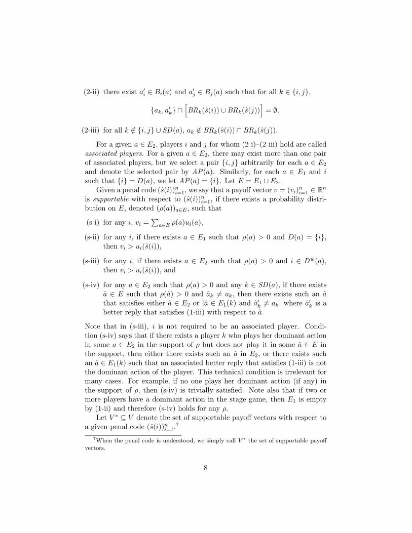
For a given a ∈ E2, players i and j for whom (2-i)–(2-iii) hold are calledassociated players. For a given a ∈ E2, there may exist more than one pairof associated players, but we select a pair {i, j} arbitrarily for each a ∈ E2

and denote the selected pair by AP(a). Similarly, for each a ∈ E1 and isuch that {i} = D(a), we let AP(a) = {i}. Let E = E1 ∪ E2.

Given a penal code (s(i))ni=1, we say that a payoff vector v = (vi)n

i=1 ∈ Rn

is supportable with respect to (s(i))ni=1, if there exists a probability distri-

bution on E, denoted (ρ(a))a∈E , such that

(s-i) for any i, vi =∑

a∈E ρ(a)ui(a),

(s-ii) for any i, if there exists a ∈ E1 such that ρ(a) > 0 and D(a) = {i},then vi > ui(s(i)),

(s-iii) for any i, if there exists a ∈ E2 such that ρ(a) > 0 and i ∈ Dw (a),then vi > ui(s(i)), and

(s-iv) for any a ∈ E2 such that ρ(a) > 0 and any k ∈ SD(a), if there existsa ∈ E such that ρ(a) > 0 and ak �= ak, then there exists such an athat satisfies either a ∈ E2 or [a ∈ E1(k) and a′k �= ak] where a′k is abetter reply that satisfies (1-iii) with respect to a.

Note that in (s-iii), i is not required to be an associated player. Condi-tion (s-iv) says that if there exists a player k who plays her dominant actionin some a ∈ E2 in the support of ρ but does not play it in some a ∈ E inthe support, then either there exists such an a in E2, or there exists suchan a ∈ E1(k) such that an associated better reply that satisfies (1-iii) is notthe dominant action of the player. This technical condition is irrelevant formany cases. For example, if no one plays her dominant action (if any) inthe support of ρ, then (s-iv) is trivially satisfied. Note also that if two ormore players have a dominant action in the stage game, then E1 is emptyby (1-ii) and therefore (s-iv) holds for any ρ.

Let V ∗ ⊆ V denote the set of supportable payoff vectors with respect toa given penal code (s(i))n

i=1.7

7When the penal code is understood, we simply call V ∗ the set of supportable payoffvectors.

8

4 A Characterization of Equilibrium Payoff Vec-tors

We are now ready to state our main result, which gives a sufficient conditionfor a given payoff vector to be approximated by a sequential equilibriumwhen the observation costs (λi)n

i=1 are sufficiently small and the discountfactors (δi)n

i=1 are sufficiently close to one.

Proposition 1 Let (s(i))ni=1 be a penal code and V ∗ be the set of supportable

payoff vectors with respect to the penal code. Then for any v ∈ V ∗ and anyε > 0, there exist λ = (λi)n

i=1 ∈ Rn++ and δ = (δi)n

i=1 ∈ (0, 1)n such that, forany game Γ(δ, λ) with δ ≥ δ and λ ≤ λ, there exists a sequential equilibriumσ∗ that satisfies |gi(σ∗) − vi| < ε for any i.

Proof. See the Appendix.

While the proof in the Appendix provides a general construction of anequilibrium that approximates a given supportable payoff vector, we heregive its main idea, restricting ourselves to special examples of supportablepayoff vectors. Let us begin with the simplest case, which is to approximatea payoff vector that is equal to u(a) for some a ∈ E2 such that Dw (a) ={1, 2, . . . , n}. Since a ∈ E2, there exist a pair of associated players {i, j} =AP(a) and better replies {a′i, a′j} of them such that (2-i)–(2-iii) hold. SinceDw (a) = {1, 2, . . . , n}, supportability implies vk > uk(s(k)) for all k. Thusthe penal code Nash equilibrium for player k, s(k), indeed makes k suffer.

To simplify our exposition, we call action ak “cooperation,” action a′kgiven by (2-ii) “minor-deviation,” and any other action “major-deviation.”Note that only the associated players {i, j} = AP(a) can minor-deviate.

We construct a strategy profile that uses n + 1 states. The set of statesis {0, 1, . . . , n}. State 0 is regarded as the cooperative state, in which (i)each player k ∈ {i, j} randomizes between cooperation and minor-deviation,where the probability of cooperation is sufficiently close to 1, (ii) all otherplayers k /∈ {i, j} cooperate, and (iii) all players monitor the other players.On the other hand, in state i ≥ 1, player i is punished; the players play s(i)and no one monitors the others.

We now specify the rule that governs the transition of states. The initialstate is 0 (cooperative state). If the state is 0 in period t − 1, then period tis in

(i) state k if player k ∈ {1, . . . , n} is the only player who major-deviated,

9

(ii) state k if player k ∈ {i, j} minor-deviated and all other players coop-erated, and

(iii) state 0 otherwise.

For any k ≥ 1, if the state moves to k because of a unilateral major-deviationof player k (case (i)), then the state remains k for all subsequent periods.On the other hand, if the state moves to k because of a unilateral minor-deviation of player k ∈ {i, j} (case (ii)), then state remains k for a certainnumber of periods and then moves back to 0. The length of the k-stateperiods is set so that the gain from the minor-deviation is exactly equal tothe loss from playing s(k). Since uk(a) > uk(s(k)), the appropriate length ofthe k-state periods can be found if the players are sufficiently patient. Sincethe appropriate length is not necessarily an integer, the public randomiza-tion device is used to make the transition from state k to 0 contingent onsunspots. Moreover, since when the state moves back to 0 depends onlyon sunspots, the state is common knowledge although the players do notmonitor each other during the punishment periods.

This specification is sufficient to determine what happens on the path.Since the players cooperate with a probability sufficiently close to 1, thepath approximates the payoff vector u(a) as long as the observation costsare sufficiently small. Note that the above specification also determinesthe continuation play at off-the-path histories if the player did not deviatein terms of monitoring in the previous periods (since then she knows thestate). To define the equilibrium strategy formally, it remains to specifyhow a player behaves after she deviates in terms of monitoring. However,since this specification does not affect the following argument, we do notcomplete the specification of strategy here.

Let us now examine the incentive to follow the state-dependent play de-scribed above. First, for δ sufficiently close to the unit vector, no player hasan incentive to major-deviate in state 0. This is because uk(a) > uk(s(k))for all k and once player k major-deviates, the resulting outcome is theperpetual play of s(k). Second, players k ∈ {i, j} are indifferent betweencooperation and minor-deviation because of the way in which the numberof k-state periods is set. Third, in state k ≥ 1, no player has an incentive todeviate in terms of action or monitoring since (i) a stage game Nash equilib-rium is played, (ii) the play does not affect the transition of the state, and(iii) no monitoring is required.

The remaining step is to examine the monitoring incentive in state 0.We start with players k /∈ {i, j}. Suppose that the state was 0 in period tand player k /∈ {i, j} did not monitor at the end of the period. Then,

10

in period t + 1, she is uncertain about the state, which is either 0, i, or jdepending on whether i or j (or both) minor-deviated in period t. By (2-iii),playing ak in period t + 1 is not optimal if the state is either i or j. On theother hand, if player k plays an action other than ak in period t+1, the actionis considered as a major-deviation and triggers a perpetual punishment ifthe state is actually 0. Therefore, if λk is sufficiently small, the gain fromeliminating the uncertainty exceeds the cost of monitoring.

Let us now consider a player k ∈ {i, j}. Without loss of generality, letk = i. Suppose that the state was 0 in period t and player i did not monitorat the end of the period, so i is uncertain about the state in period t + 1.First, consider the case in which player i cooperated in period t. Then thestate in period t + 1 is either j or 0 depending on the action of player jin period t. Thus, if i cooperates or minor-deviates in period t + 1, thenby (2-ii), the action is suboptimal if the state is j. On the other hand,if i major-deviates in period t + 1, a perpetual punishment follows if theactual state is 0. Hence, player i suffers strictly from the uncertainty andit is optimal for her to eliminate the uncertainty if her monitoring cost issufficiently small.

Let us now consider the case when player i minor-deviated in period t.Then the state in period t + 1 is either i or 0; the latter occurs if j alsominor-deviated. Since the latter case occurs with a small probability, thestate in period t + 1 is almost surely i, so by (2-ii), it is suboptimal for i toeither cooperate or minor-deviate in period t + 1. However, if she choosesan action other than cooperation and minor-deviation in period t + 1, thenit is regarded as a major-deviation if the state in this period is actually 0,which occurs with a small but positive probability. Thus, player i suffersstrictly from the uncertainty, which she is willing to avoid if her monitoringcost is sufficiently small.

In this way, we can prove that it is not profitable for players to devi-ate in terms of monitoring (on the path). This together with the previousarguments shows that the state-dependent play is an equilibrium when theplayers are patient and monitoring costs are small.

It is less straightforward to approximate other supportable payoff vec-tors. For example, let us consider a payoff vector that is equal to u(a) forsome a ∈ E1. By (1-i), only one player has a short-run incentive to deviatefrom a. The state-dependent play described above cannot be used since itrequires two players to minor-deviate (to give monitoring incentives to eachof them). Therefore, we consider a different type of behavior in this case.Specifically, in the cooperative state, the player i such that D(a) = {i}randomizes between cooperation and minor-deviation and does not monitor

11

the other players, while all other players cooperate and monitor the others.The state transition is specified similarly. Then, all agents j �= i have amonitoring incentive in the cooperative state since the future play is eitherto cooperate or to punish i and the state transition depends on i’s action.On the other hand, since the state transition depends only on i’s action, ican identify the current state even if she does not monitor the other players.Thus, at equilibrium, the state is common knowledge among the playersalthough not all players observe the past actions.

The construction of an equilibrium is more complicated if the payoffvector to be approximated can be generated only by a randomization amongelements of E1 and E2, or when some players play a dominant action in thecooperative stage. We deal with these cases in the Appendix.

A final remark on Proposition 1 is that if the players use sunspots wisely,many other payoff vectors can be approximated. Let NE ∗(G) be the set ofNash equilibrium payoff vectors of G. Then it is easily seen that any payoffvector in the convex hull of V ∗ ∪ NE ∗(G) can be approximated. Moreover,as we vary the penal code (s(i))n

i=1, we obtain different V ∗ and thereforedifferent V ∗ ∪NE ∗(G), and all elements of those sets can be approximated.Thus, if G has a number of Nash equilibria, the set of payoff vectors thatour construction can approximate can be large.8 In the next section, wedemonstrate that the set is indeed large and yields an approximate FolkTheorem.

5 Application: Approximate Folk Theorem

This section examines three examples and shows that Proposition 1 gener-ates an approximate Nash Folk Theorem in each of the examples. In theseexamples, we consider a penal code in which the same Nash equilibrium isused for all players. Denoting the stage Nash equilibrium by s, we will showthat all efficient payoff vectors that Pareto-dominate u(s) are supportablewith respect to s. Then, Proposition 1 proves that all those payoff vectorsare approximated by equilibria if the monitoring costs are sufficiently small.Since sunspots are available, all interior payoff vectors that Pareto-dominateu(s) are also attainable as equilibria. In this way, we obtain an approximateNash Folk Theorem. A minimax version of approximate Folk Theorem mayalso hold if, in addition, ui(s) is the minimax value of player i for all i.We indeed obtain an approximate minimax Folk Theorem in the example of

8Furthermore, there may be payoff vectors that can be supported by other strategyprofiles than the ones we consider in this paper.

12

linear partnership examined below.

5.1 A Variant of Prisoners’ Dilemma

We begin our discussion with the following standard prisoners’ dilemma.

C DC 1, 1 −1, 2D 2,−1 0, 0

If this is the stage game, then our construction of strategy profile cannotsupport cooperation. Indeed, since the Nash equilibrium is unique, the onlypossible penal code is s(1) = s(2) = (D, D). Then, (C, C) violates (1-i) and(2-ii). Condition (2-ii) is simply impossible to satisfy if there are only twoactions. Similarly, (C, D) and (D, C) violate (1-ii) and (2-i). Thus E1 andE2 are empty for the prisoners’ dilemma.

On the other hand, the result changes considerably if the stage gamehas a slightly larger action set. For prisoners’ dilemma, our constructioncan easily support cooperation if each player has another action. This isillustrated by the following stage game.

C D EC 1, 1 −1, 2 −1,−1D 2,−1 0, 0 −1,−1E −1,−1 −1,−1 0, 0

This is a simplified version of the bilateral trade game with moral hazard inBhaskar and van Damme (2002). This game has two pure Nash equilibria,(D, D) and (E, E), as well as a mixed Nash equilibrium, s, where each playerrandomizes between D and E with equal probabilities. Clearly, C is strictlydominated, and (C, C) Pareto-dominates all Nash equilibria.

We present an approximate Nash Folk Theorem for the expanded pris-oners’ dilemma. We set s(1) = s(2) = (E, E) as a penal code. Then, sinceneither C nor D is a best response to E, we have (C, C) ∈ E2. Further-more, since D is a unique best response to C, we also have (C, D) ∈ E1 and(D, C) ∈ E1. Since no player has a dominant action, Condition (s-iv) ofsupportability holds trivially. Since (C, C), (D, C), and (C, D) are the onlyefficient action profiles, any efficient payoff vector that Pareto-dominates(0, 0) is supportable and therefore approximated by an equilibrium. Thusan approximate Nash Folk Theorem holds.

However, this is not an approximate minimax Folk Theorem since theminimax value in this game is −1/2 for each player. The fact that the

13

minimax value is attained by the mixed Nash equilibrium s does not enableus to prove a minimax Folk Theorem. Indeed, if we set s(1) = s(2) = sas a penal code, then E1 and E2 are both empty, and so is the set ofsupportable payoff vectors with respect to the penal code. This argumentalso demonstrates that the set of supportable payoff vectors depends on thepenal code.

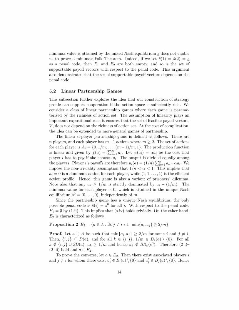
5.2 Linear Partnership Games

This subsection further explores the idea that our construction of strategyprofile can support cooperation if the action space is sufficiently rich. Weconsider a class of linear partnership games where each game is parame-terized by the richness of action set. The assumption of linearity plays animportant expositional role; it ensures that the set of feasible payoff vectors,V , does not depend on the richness of action set. At the cost of complication,the idea can be extended to more general games of partnership.

The linear n-player partnership game is defined as follows. There aren players, and each player has m+1 actions where m ≥ 2. The set of actionsfor each player is Ai = {0, 1/m, . . . , (m−1)/m, 1}. The production functionis linear and given by f(a) =

∑ni=1 ai. Let ci(ai) = αai be the cost that

player i has to pay if she chooses ai. The output is divided equally amongthe players. Player i’s payoffs are therefore ui(a) = (1/n)

∑nk=1 ak−αai. We

impose the non-triviality assumption that 1/n < α < 1. This implies thatai = 0 is a dominant action for each player, while (1, 1, . . . , 1) is the efficientaction profile. Hence, this game is also a variant of prisoners’ dilemma.Note also that any ai ≥ 1/m is strictly dominated by ai − (1/m). Theminimax value for each player is 0, which is attained in the unique Nashequilibrium s0 = (0, . . . , 0), independently of m.

Since the partnership game has a unique Nash equilibrium, the onlypossible penal code is s(i) = s0 for all i. With respect to the penal code,E1 = ∅ by (1-ii). This implies that (s-iv) holds trivially. On the other hand,E2 is characterized as follows.

Proposition 2 E2 = {a ∈ A : ∃i, j �= i s.t. min{ai, aj} ≥ 2/m}.

Proof. Let a ∈ A be such that min{ai, aj} ≥ 2/m for some i and j �= i.Then, {i, j} ⊆ D(a), and for all k ∈ {i, j}, 1/m ∈ Bk(a) \ {0}. For allk /∈ {i, j} ∪ SD(a), ak ≥ 1/m and hence ak /∈ BRk(s0). Therefore (2-i)–(2-iii) hold and a ∈ E2.

To prove the converse, let a ∈ E2. Then there exist associated players iand j �= i for whom there exist a′i ∈ Bi(a) \ {0} and a′j ∈ Bj(a) \ {0}. Hence

14

min{ai, aj} ≥ 2/m. Q.E.D.

Let V be the boundary of V , and VIR ⊆ V be the set of feasible payoffvectors that are strictly individually rational, i.e., VIR = {v ∈ V : vi >0 for all i}. Since payoff functions are linear, V , V , and VIR are all in-dependent of m. The following result proves that all feasible, boundary,and strictly individually rational payoff vectors are supportable if m is suf-ficiently large. In view of Proposition 1 and the availability of sunspots, theresult implies that if m is large, any v ∈ VIR can be approximated by anequilibrium. Therefore, we have an approximate minimax Folk Theorem.

Proposition 3 If m ≥ 2/(nα − 1), any v ∈ VIR ∩ V is supportable.

Proof. Assume m ≥ 2/(nα − 1) and let v ∈ VIR ∩ V . Then there existsa probability distribution on A, (ρ(a))a∈A, such that v =

∑a∈A ρ(a)u(a).

Let ρ∗i =∑

a∈A ρ(a)ai, which is the expected action level of player i. Sincev ∈ VIR ∩ V , there exists a player i such that ρ∗i = 1 (otherwise, a Paretoimprovement can be achieved by multiplying everyone’s expected actionlevel by some β > 1). Without loss of generality, we assume ρ∗1 = 1. If∑

k≥2 ρ∗k < 2/m, then the expected utility of player 1 is

v1 = (1/n)n∑

i=1

ρ∗i − α < (1/n)(1 + 2/m) − α ≤ 0,

where the last inequality follows from m ≥ 2/(nα − 1). The inequalitiesimply that v is not strictly individually rational, a contradiction. Thus∑

k≥2 ρ∗k ≥ 2/m.We have to show that there exists a probability distribution over E2

that generates payoff vector v. Since payoff functions are linear, it sufficesto prove that the convex hull of E2 includes ρ∗ = (ρ∗i )

ni=1. To prove this, let

βH and βL be defined by

βH = 1/(maxk≥2

ρ∗k) ≥ 1, (2)

βL = (2/m)/∑k≥2

ρ∗k ≤ 1, (3)

where the inequality in (3) is proved in the previous paragraph. Let ρH , ρL ∈[0, 1]n be defined by ρH

1 = ρL1 = 1, and for all k ≥ 2, ρH

k = βHρ∗k andρL

k = βLρ∗k. Clearly, ρ∗ is a convex combination of ρH and ρL. By (2), ρH

has at least two components of 1. Thus, it follows easily from Proposition 2

15

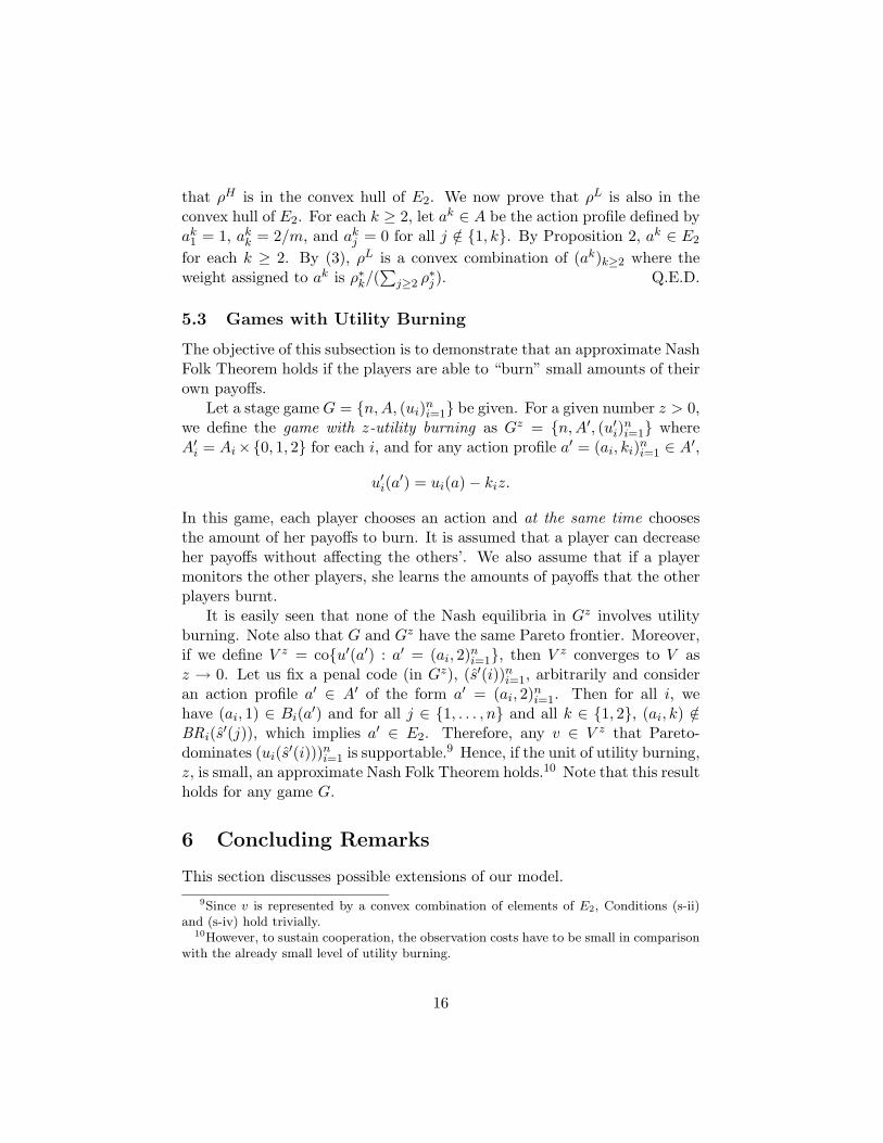
that ρH is in the convex hull of E2. We now prove that ρL is also in theconvex hull of E2. For each k ≥ 2, let ak ∈ A be the action profile defined byak

1 = 1, akk = 2/m, and ak

j = 0 for all j /∈ {1, k}. By Proposition 2, ak ∈ E2

for each k ≥ 2. By (3), ρL is a convex combination of (ak)k≥2 where theweight assigned to ak is ρ∗k/(

∑j≥2 ρ∗j ). Q.E.D.

5.3 Games with Utility Burning

The objective of this subsection is to demonstrate that an approximate NashFolk Theorem holds if the players are able to “burn” small amounts of theirown payoffs.

Let a stage game G = {n, A, (ui)ni=1} be given. For a given number z > 0,

we define the game with z-utility burning as Gz = {n, A′, (u′i)

ni=1} where

A′i = Ai ×{0, 1, 2} for each i, and for any action profile a′ = (ai, ki)n

i=1 ∈ A′,

u′i(a

′) = ui(a) − kiz.

In this game, each player chooses an action and at the same time choosesthe amount of her payoffs to burn. It is assumed that a player can decreaseher payoffs without affecting the others’. We also assume that if a playermonitors the other players, she learns the amounts of payoffs that the otherplayers burnt.

It is easily seen that none of the Nash equilibria in Gz involves utilityburning. Note also that G and Gz have the same Pareto frontier. Moreover,if we define V z = co{u′(a′) : a′ = (ai, 2)n

i=1}, then V z converges to V asz → 0. Let us fix a penal code (in Gz), (s′(i))n

i=1, arbitrarily and consideran action profile a′ ∈ A′ of the form a′ = (ai, 2)n

i=1. Then for all i, wehave (ai, 1) ∈ Bi(a′) and for all j ∈ {1, . . . , n} and all k ∈ {1, 2}, (ai, k) /∈BRi(s′(j)), which implies a′ ∈ E2. Therefore, any v ∈ V z that Pareto-dominates (ui(s′(i)))n

i=1 is supportable.9 Hence, if the unit of utility burning,z, is small, an approximate Nash Folk Theorem holds.10 Note that this resultholds for any game G.

6 Concluding Remarks

This section discusses possible extensions of our model.9Since v is represented by a convex combination of elements of E2, Conditions (s-ii)

and (s-iv) hold trivially.10However, to sustain cooperation, the observation costs have to be small in comparison

with the already small level of utility burning.

16

6.1 Fixed Observation Costs

An important assumption in our characterization of equilibrium payoff vec-tors and approximate Folk Theorems is that the observation costs are suffi-ciently small. The results say nothing if the levels of observation costs arefixed. A simple, alternative framework in which we can deal with fixed levelsof observation costs is one in which monitoring at the end of a period givesinformation about not only the present period but all the previous periods.This framework is a variation of that in Miyahara (2002), who examinesthe case when at least the last two periods can be observed. However,Miyahara’s efficiency result for repeated prisoners’ dilemma also requiressmall observation costs.

When all previous periods are observable (with costs), we can useMiyahara’s construction of strategy profile to support a large set of pay-off vectors for fixed observation costs. To see this, assume that there existsan action profile a that attains a given target payoff vector. Let us alsoassume the existence of an action profile a in which there exist at least twopotential deviators, i.e., |D(a)| ≥ 2. As in our construction, select two play-ers {i, j} ⊆ D(a) and call them the associated players. Then consider thefollowing strategy profile for a given T ∈ {2, 3, . . .}: (i) the players play ain the first T − 1 periods without monitoring each other; (ii) in period T ,the players play a, except that the associated players mix between a andtheir minor-deviations, and all players monitor; (iii) the play in the next Tperiods is either another sequence of (i) and (ii), or a repetition of a penalcode Nash equilibrium, depending on the presence of a deviator in the firstT periods, and so on.

Under the strategy profile, the players do not monitor the other playersin a state. But they have no incentive to deviate in terms of actions sincedeviations are detected at least T periods later and regarded as major-deviations. The incentive for monitoring in period T is guaranteed if foreach player k, ak is not a best response to the penal code Nash equilibriadesigned for the associated players. Under this condition, the above strategyprofile constitutes an equilibrium and approximates the target payoff vectorfor a given vector of observation costs if T is sufficiently large and discountfactors are close to 1.11

11In the strategy profile, the action profile is the same for the first T − 1 periods.Alternatively, we could consider a strategy profile in which the action profile during theseperiods is time-dependent. The advantage of using the larger class of strategy profiles isthat the corresponding condition on the relation between “a” and the penal code can beweakened considerably.

17

This construction for multi-period observation technology can sustaincooperation even for stage games whose action sets are small. Indeed, thestage game examined in Miyahara (2002) is the standard two-action prison-ers’ dilemma and he obtains an efficiency result for the game.

In our future research, we will elaborate the strategy profile (along theline mentioned in footnote 11) to obtain a characterization of payoff vectorsthat can be approximated by equilibria and derive conditions on stage gamesfor which a Folk Theorem with fixed observation costs holds.

6.2 Timing of Receiving Payoffs

We have assumed that the players do not receive payoffs in each periodbut they receive the total payoffs when the game ends. We need theseassumptions in order to keep consistency with the assumption that, withoutpaying monitoring costs, a player receives no information about the others’actions. If payoffs are received in every period, then they generally provideplayers with some information about the other players’ actions.

However, we can imagine a framework in which payoffs are received inevery period but monitoring remains important because realized payoffs areonly a noisy signal of the other players’ actions. For example, let a stagegame G = {n, A, (ui)n

i=1} be given. Suppose that at the end of each period,player i receives payoffs of ui(a)+ εi if a ∈ A is played in that period, whereεi is a noise term which follows a normal distribution with mean 0. Assumealso that the noise terms are independent across the players.

In this formulation, the realized payoff is not a sure indicator of theother players’ actions while it is informative. If we ignore the issue of costlyobservation, the standard model of repeated games with imperfect privatemonitoring (like Sekiguchi (1997)) falls into this category if the realizedpayoff is a sufficient statistic of the privately observed signal about the otherplayers’ actions.

Even in this framework, we can use the state-dependent strategy profileconsidered in Section 4. Under this strategy profile, players monitor eachother and do not use the information contained in the realized payoffs. Themonitoring incentive is weaker under this strategy profile since realized pay-offs also give players information about the state. However, players who donot pay observation costs are not able to determine the state with certainty.Therefore, if the likelihood ratio of any pair of action profiles that generatethe same level of payoffs is bounded away from zero, then the players dohave an incentive to pay observation costs, given any payoff realization, if

18

the observation costs are sufficiently small.12 Hence the basic idea of ourconstruction also applies to the case in which payoffs are received in eachperiod.

This observation is important because it suggests a possibility that costlyobservation is one comprehensive solution to the private monitoring prob-lem. The literature of repeated games with imperfect private monitoringhas shown difficulty in constructing a cooperative/efficient equilibrium, andthe existing positive results (reported in the papers cited in footnote 2) arelimited to simple specific games, e.g., repeated prisoners’ dilemma and itsvariations.13 It is still unknown whether a Folk Theorem or an efficiencyresult holds in general settings with private monitoring. In contrast, ourresult and the above discussions show that an approximate Folk Theoremdoes hold in general environments if the players have an ability to observethe other players’ actions directly and the observation costs are sufficientlysmall.

The literature also identifies communication among the players as a driv-ing force to cooperation in general environments with private monitoring(Compte (1998), Kandori and Matsushima (1998), and Aoyagi (2002)).14

Thus our analysis may as well be seen as demonstrating that costly obser-vation is a convenient substitute for communication. This interpretationhas a strong implication on antitrust laws since they control communicationamong firms in the belief that communication is a major tool that facilitatescartels.

6.3 Partial Monitoring

The monitoring activity that we have considered has a binary aspect in thateach player has to decide whether to obtain complete information about theaction profile of the other players in the period or to obtain no information.

A more realistic formulation is that each player can choose to whatextent she observes the other players’ actions, and the more she spends for

12Precisely speaking, the likelihood ratio is not bounded away from zero when the noiseterms are normally distributed. However, the likelihood ratio is close to zero only atthe tails. Hence, we conjecture that there exists a cooperative equilibrium in which theplayers monitor each other unless the realized payoffs take extreme values. Moreover, thelikelihood ratio condition can be satisfied for other specifications of the noise term.

13Mailath and Morris (2002) consider more general stage games, but they assume thatprivate signals are correlated across the players. Amarante (2002) also conducts a generalanalysis. For some negative results, see Matsushima (1991) and Compte (2002).

14See also Ben-Porath and Kahneman (1996) for the role of communication in relatedenvironments with private monitoring.

19

monitoring, the more information she obtains. For example, suppose thatλi is the unit monitoring cost and player i incurs the cost of mλi if shemonitors m of the other players. This alternative framework is relevant inthe price-setting oligopoly if the goods are sold at each firm’s own outlet.In this framework, each firm decides the set of firms to monitor and thetotal observation cost depends on the number of firms to monitor. Suchpartial monitoring is relevant even in the case of duopoly if the firms operatein multiple markets. In this case, each firm decides the set of markets tomonitor, and the total observation cost depends on the number of markets tomonitor. Thus the price-setting oligopoly is a prominent example of partialmonitoring since the firms often compete in a large number of dimensions.As Stigler (1964) concluded, collusion is hard to implement since it requiresan ability to detect any possible secret price-cuts in any market.

In general, partial monitoring is relevant whenever the action profile ofn − 1 players is multi-dimensional (this is trivially the case when n ≥ 3)and a player can choose to observe only a subset of the coordinates in theprofile of the other players’ actions. A basic difficulty in analyzing the casewhen partial monitoring is feasible is that the players have an incentive toeconomize on observation expenses by not monitoring some of the players(or markets). In the strategy profile used in our proof, some of the playersdo not randomize in the cooperative state, but this is not a problem in theproof since these players are also monitored by the other players. Under thebinary nature of our monitoring technology, any player who has an incentiveto monitor at least one of the other players has no choice but to monitorall other players. However, if partial monitoring is feasible, players wouldmonitor only those who randomize, but then deviations of non-randomizingplayers are not detected. Therefore, if partial monitoring is feasible, thecooperative equilibria that we constructed are upset.

Nevertheless, our construction can be modified to deal with partial mon-itoring if the payoff vector to be approximated can be generated by actionprofiles in which all players have proper minor-deviations. Formally, let astage game G and a penal code (s(k))n

k=1 be given. Let En ⊆ A be the setof all a ∈ A such that

(n-i) D(a) = {1, 2, . . . , n},(n-ii) for each player i, there exists a′i ∈ Bi(a) such that

{ai, a′i} ∩

[∪n

k=1BRi(s(k))]

= ∅.

20

It is then not very difficult to see that for all a ∈ En, if ui(a) > ui(s(i))for all i, then u(a) can be approximated by an equilibrium, in which allplayers randomize between ai and a′i in the cooperative state. Thus, anyconvex combination of such u(a)’s can be also approximated. We have seenin Subsection 5.2 that the finer the action set is, the more payoff vectorsare approximated using action profiles where all players have short-run in-centives to deviate. Therefore, our result extends to the case of partialmonitoring when the underlying strategic situation involves sufficiently fineaction sets.

This idea also applies to the case of duopoly with multiple markets. If aprice profile is such that each firm has a short-run incentive to deviate in ev-ery market, then the price profile can be supported by an equilibrium wherethe firms randomize between cooperation and minor-deviation in every mar-ket. Again, if the price space is sufficiently fine, many levels of collusion canbe sustained, so an approximate Folk Theorem will be obtained.

6.4 Finite Repetition

Assuming that the horizon is finite has both an advantage and a disadvan-tage. An advantage is that the finite horizon makes it easier to interpretthe assumption that the payoffs are received in total at the end of the re-peated game. A disadvantage is that the finite horizon makes cooperationunsustainable if the stage game has a unique equilibrium.

On the other hand, it might be possible to obtain an approximate FolkTheorem under a finite horizon if the stage game has multiple equilibriumpayoffs for each player as in Benoit and Krishna (1985). We conjecture thatif the number of periods is sufficiently large, an action profile that Pareto-dominates a stage-game equilibrium can be sustained in early periods. Thisis another topic of our future research.

21

Appendix: Proof of Proposition 1

Let v ∈ V ∗ and ε > 0. Since v is supportable, there exists a probabilitydistribution on E, denoted (ρ(a))a∈E , such that (s-i)–(s-iv) hold. Let usdefine E∗

1(i) = {a ∈ E1 : ρ(a) > 0 and D(a) = {i}}, E∗1 = ∪iE

∗1(i), E∗

2 ={a ∈ E2 : ρ(a) > 0}, and E∗ = E∗

1 ∪ E∗2 . Thus, E∗ is the support of ρ.

We can choose a sufficiently small ε > 0 so that for all players i, if thereexists a ∈ E∗ such that either [a ∈ E1 and D(a) = {i}] or [a ∈ E2 andi ∈ Dw (a)], then vi − ε > ui(s(i)). This is possible since v is supportable.

Let SD∗ = {i : i ∈ SD(a) ∀a ∈ E∗} be the set of players i such thatfor all a, a ∈ E∗, ai = ai and it is the strictly dominant action for i.

For each i and a ∈ E∗1(i), fix a′i ∈ Bi(a) such that (1-iii) and (s-iv) hold.

Similarly, for each a ∈ E∗2 , we fix a′i ∈ Bi(a) and a′j ∈ Bj(a) that satisfy

(2-ii), where {i, j} = AP(a).Since G is a finite game, there exists ζ ∈ (0, 1) such that for all a ∈ E∗

1 ,(1-iii) holds with ζ = ζ, and for all a ∈ E2 and all k /∈ Dw (a),

{ak} = BRk((1 − ζ)ai + ζa′i, (1 − ζ)aj + ζa′j , a−i−j), (4)

where {i, j} = AP(a). Note that these conditions also hold when ζ isreplaced with any ζ ∈ [0, ζ).

Let η ∈ [0, ζ], λi ≥ 0, and δi ∈ (0, 1) for all i. For any a ∈ E∗ and anyk ∈ AP(a), we define a mixed action aη

k as

aηk = (1 − η)ak + ηa′k,

with the obvious interpretation that aηk assigns probability 1 − η to ak and

the remaining probability to a′k. We now define the following vectors andnumbers: V 0 ∈ R

n, V 0(a) ∈ Rn, V k(a) ∈ R

n, and νk(a) ∈ (0, 1) for anya ∈ E∗ and any k ∈ AP(a). We define them as a solution of the followingsystem:

V 0 =∑

a∈E∗ρ(a)V 0(a); (5)

V 0i (a) = (1 − δi)ui(a) + δiV

0i (6)

= (1 − δi)ui(a′i, a−i) + δiVii (a) (7)

for any i and any a ∈ E∗1(i);

V 0k (a) = (1 − δk)

[uk(a

ηi , a−i) − λk

]+ δk

[(1 − η)V 0

k + ηV ik (a)

](8)

22

for any i, any a ∈ E∗1(i), and any k �= i;

V i(a) = [1 − νi(a)]u(s(i)) + νi(a)V 0 (9)

for any i and any a ∈ E∗1(i);

V 0i (a) = (1 − δi)

[ui(a

ηj , a−j) − λi

]+ δi

[(1 − η)V 0

i + ηV ji (a)

](10)

= (1 − δi)[ui(a′i, a

ηj , a−i−j) − λi

]+ δi

[(1 − η)V i

i (a) + ηV 0i

](11)

and

V 0j (a) = (1 − δj)

[uj(a

ηi , a−i) − λj

]+ δj

[(1 − η)V 0

j + ηV ij (a)

](12)

= (1 − δj)[uj(a′j , a

ηi , a−i−j) − λj

]+ δj

[(1 − η)V j

j (a) + ηV 0j

](13)

for any a ∈ E∗2 and the associated players {i, j} = AP(a);

V 0k (a) = (1 − δk)

[uk(a

ηi , a

ηj , a−i−j) − λk

]

+ δk

{[(1 − η)2 + η2

]V 0

k + η(1 − η)[V i

k (a) + V jk (a)

]}(14)

for any a ∈ E∗2 , any k /∈ AP(a) ∪ SD∗, and {i, j} = AP(a);

V 0k (a) = (1 − δk)uk(a

ηi , a

ηj , a−i−j)

+ δk

{[(1 − η)2 + η2

]V 0

k + η(1 − η)[V i

k (a) + V jk (a)

]}(15)

for any a ∈ E∗2 , any k ∈ SD∗ (note that AP(a) ∩ SD∗ = ∅ by (2-i)), and

{i, j} = AP(a); and

V k(a) = [1 − νk(a)]u(s(k)) + νk(a)V 0 (16)

for any a ∈ E∗2 and any k ∈ AP(a).

Regarding system (5)–(16), we prove the following lemma.

Lemma 1 There exist η ∈ (0, ζ], λ > 0, κ > 0, and δ ∈ (0, 1) such that

(i) System (5)–(16) has a solution if η ≤ η, λi ≤ λ, and δi ≥ δ for any i.

(ii) The solution satisfies

|V 0i − vi| < ε (17)

for any i, and

1 − νk(a)1 − δk

> κ (18)

for any a ∈ E∗ and any k ∈ AP(a).

23

Proof. We first examine system (5)–(16) when η = λi = 0 for any i. By(5), (6), (8), (10), (12), (14), and (15), any solution satisfies

V 0i = vi (19)

V 0i (a) = (1 − δi)ui(a) + δivi

for any a ∈ E∗ and any i. Therefore, (6), (7), and (9) reduce to

(1 − δi)[ui(a′i, a−i) − ui(a)

]= δi(1 − νi(a))

[vi − ui(s(i))

](20)

for any i and a ∈ E∗1(i). Since v is supportable, vi > ui(s(i)). Since

a′i ∈ Bi(a), (20) has a unique solution νi(a) ∈ (0, 1) if δi is sufficiently closeto 1. By (9) and (19), this solution uniquely determines V i(a). Furthermore,(20) yields

1 − νi(a)1 − δi

>ui(a′i, a−i) − ui(a)

vi − ui(s(i)). (21)

Similarly, for any a ∈ E∗2 , (10)–(13) and (16) reduce to

(1 − δk)[uk(a′k, a−k) − uk(a)

]= δk(1 − νk(a))

[vk − uk(s(k))

](22)

for all k ∈ {i, j} = AP(a). Since {i, j} ⊆ D(a) and v is supportable,vk > uk(s(k)) for all k ∈ {i, j}. Since a′k ∈ Bk(a) for all k ∈ {i, j}, (22) hasa unique solution (νi(a), νj(a)) ∈ (0, 1)2 if δi and δj are both sufficiently closeto 1. By (16), the solution uniquely determines V i(a) and V j(a). Moreover,(22) yields

1 − νk(a)1 − δk

>uk(a′k, a−k) − uk(a)

vk − uk(s(k))(23)

for all k ∈ AP(a).Hence, if η = λi = 0 for all i, then there exists δ ∈ (0, 1) such that if

δi ≥ δ for all i, then system (5)–(16) has a unique solution satisfying (17).Moreover, if we choose

κ = (1/2) mina∈E∗

k∈AP(a)

[uk(a′k, a−k) − uk(a)vk − uk(s(k))

]> 0,

then (21) and (23) imply that (18) holds for all a ∈ E∗ and all k ∈ AP(a).By the standard continuity argument, there exist η ∈ (0, ζ], λ > 0, and

δ ∈ (0, 1) such that if η ≤ η, λi ≤ λ, and δi ≥ δ for all i, then system(5)–(16) has a nearby solution satisfying (17) and (18). Q.E.D.

24

For any player k, if BRk(s(i)) �= Ak for some i, then let

pk = min{uk(s(i)) − uk(ak, s−k(i)) :i ∈ {1, . . . , n} and ak /∈ BRk(s(i))

}> 0.

That is, any player k who plays a suboptimal action against a penal codeNash equilibrium loses at least pk in terms of per-stage payoffs.

For any player k, if k /∈ D(a) for some a ∈ E∗1 , then let

rk = min{uk(a) − uk(ak, a−k) :a ∈ E∗

1 , k /∈ D(a), and ak /∈ BRk(a)}

> 0.

This means that if player k such that k /∈ D(a) for some a ∈ E∗1 plays a

suboptimal action against a−k, then she loses at least rk in terms of per-stagepayoffs.

For any player k, if k /∈ (Dw (a) ∪ SD(a)) for some a ∈ E∗2 , then let

qk = min{uk(a) − uk(ak, a−k) :a ∈ E∗

2 , k /∈ (Dw (a) ∪ SD(a)), and ak �= ak

}> 0.

Thus, if player k does not play ak against a−k, then she loses at least qk interms of per-stage payoffs.

Let ρ = mina∈E∗ ρ(a) and ∆i = maxa,a′∈A(ui(a) − ui(a′)). We thenchoose η ∈ (0, η], λ = (λi)n

i=1 ∈ (0, λ]n, and δ = (δi)ni=1 ∈ [δ, 1)n that satisfy

the following inequalities:

(1 − δi + 2η)(∆i + λi) ≤ δi(1 − η)2[vi − ε − ui(s(i))

](24)

for any i such that vi − ε > ui(s(i));

λi ≤ δiρκ(η/2)(1 − η)pi (25)

for any i /∈ SD∗ such that BRi(s(k)) �= Ai for some k;

(1 − δi)λi ≤ δiρκ(η/2)[−(1 − δi + η)(∆i + λi) + δi

[vi − ε − ui(s(i))

]](26)

for any i such that i ∈ AP(a) for some a ∈ E∗2 ;

λi ≤ δiρκ(1 − η)[(1 − η)ri − η∆i

](27)

for any i such that i /∈ D(a) for some a ∈ E∗1 ; and

λi ≤ δiρκ(1 − η)2[(1 − η)2qi − [1 − (1 − η)2]∆i

](28)

25

for any i such that i /∈ (Dw (a) ∪ SD(a)) for some a ∈ E∗2 .

Let us consider Γ(δ, λ) with δ ≥ δ and λ ≤ λ. Fix η ∈ [η/2, η] andconsider the system (5)–(16) associated with η, λ, and δ. By Lemma 1, thesystem has a solution satisfying (17) and (18).

We now construct an equilibrium of Γ(δ, λ) that approximates v. Westart with describing the play on the path. The equilibrium play in each pe-riod depends on the “state” of that period. The set of states is {0, 1, . . . , n}.State 0 is called the “cooperative state,” while states i ≥ 1 are called “pun-ishment states.” State i ≥ 1 is the state in which player i is punished.

The play in state 0 is determined by the “substate” of the period, which isdetermined by the sunspot in that period. The set of substates is identifiedwith E∗, and each substate a ∈ E∗ is realized with probability ρ(a). Insubstate a ∈ E∗

1(i), (aηi , a−i) is played, while in substate a ∈ E∗

2 , aη =(aη

i , aηj , a−i−j) is played where {i, j} = AP(a). In substate a ∈ E∗

1(i), allplayers except for i monitor the other players. In substate a ∈ E∗

2 , allplayers not in SD∗ monitor the other players. This describes the play in thecooperative state. In state i ≥ 1, on the other hand, the players play s(i)and do not monitor the other players.

For future reference, given a-substate, we call action ai “cooperation,”action a′i “minor-deviation,” and any other action “major-deviation.” Notethat, according to this terminology, only player i has a minor-deviation insubstate a ∈ E∗

1(i). Likewise, in substate a ∈ E∗2 , only players i and j

associated with a can minor-deviate.Next, we define the rule that determines the transition of states. The

initial state is 0 (cooperative). If period t− 1 is in state 0 and substate a ∈E∗

1(i), then period t is in:

(i) state i if player i major- or minor-deviated in period t − 1,

(ii) state 0 otherwise.

Note that deviations of players j �= i are ignored. If period t−1 is in state 0and substate a ∈ E∗

2 , then period t is in:

(i) state k if player k ∈ Dw (a) is the only player in Dw (a) who major-deviated in period t − 1,

(ii) state k if player k ∈ {i, j} = AP(a) is the only player who minor-deviated in period t − 1 and all other players in Dw (a) cooperated inperiod t − 1,

(iii) state 0 otherwise.

26

Note that, if a ∈ E∗2 and the associated players i and j both minor-deviated,

then their deviations are ignored and the state remains 0. Any deviation ofplayer k /∈ Dw (a) is also ignored.

If the state changes to k because of player k’s major deviation, then thestate remains k in all subsequent periods. If the state changes to k because ofk’s minor deviation in a-substate, then the state remains k for τk(a) periodsirrespective of the actions during the periods. The state of the subsequentperiod depends on the sunspot at the beginning of the period: with proba-bility ξk(a), the state remains k for one more period and then moves backto 0; with probability 1−ξk(a), the state moves back to 0 immediately. Thenumbers τk(a) ∈ {0, 1, 2, . . .} and ξk(a) ∈ [0, 1) are determined uniquely by

(1 − ξk(a))δτk(a)k + ξk(a)δτk(a)+1

k = νk(a), (29)

where νk(a) is the relevant part of the solution of (5)–(16).Note that τk(a) = 0 is possible in the unique solution of (29). If this is

the case, then the state transition after player k’s unilateral minor-deviationis that with probability 1− ξk(a), the state remains 0, and with probabilityξk(a), the state stays in k for one period and then moves back to 0.

A subtle issue that arises when τk(a) = 0 is that the players seeminglyneed two sunspots: one that determines whether the state stays at 0 or movesto k, and the other that decides, if the state remains 0, which element ofE∗ is played. However, a single sunspot suffices since one can always let asunspot play two roles at the same time.15

The above description specifies only the play on the path. However,each player can follow the description as long as she does not deviate fromthe description in terms of monitoring. To see this, note first that if thecurrent period is in a-substate of the cooperative state with a ∈ E∗

1(i), thenall players except for i monitor the other players, and the future state (onthe path) depends only on i’s action (recall that deviations by player j �= iare ignored). Thus the state in the next period is common knowledge eventhough player i does not monitor the other players. Second, if the currentperiod is in substate a ∈ E∗

2 and if SD∗ = ∅, then all players monitor eachother and the state in the next period is common knowledge. If SD∗ �= ∅,then the future state is common knowledge only among the players outsideSD∗. However, this does not cause a problem since each player in SD∗ plays

15For example, suppose E∗ = {a′, a′′} and ρ(a′) = ρ(a′′) = 0.5. If τk(a) = 0 andξk(a) = 0.5, then after a minor deviation by player k in substate a, the players canarrange the next-period play so that s(k) is played if the sunspot is in [0, 0.5], a′ if it is in(0.5, 0.75], and a′′ if it is in (0.75, 1].

27

the (strictly) dominant action in all states, including the punishment states.Thus, the players in SD∗ can play consistently with the above descriptionwithout knowing the state.16 Finally, if the current state is i ≥ 1, then thefuture state depends only on sunspots and hence is common knowledge.

Let us define a strategy profile σ which is consistent with the state-dependent play described above. For each i, let Hi be the set of all historiesfor player i such that i monitored the other players whenever it was pre-scribed by the state-dependent play. Note that, as long as the players followthe state-dependent play, any history on the path is in Hi. On the otherhand, Hi includes other histories as well. It includes histories in which someplayer(s) (including i) deviated in terms of actions, and those in which imonitored the other players when she was not required to. Anyway, at anyhistory ht

i ∈ Hi, player i knows the state and therefore can follow the state-dependent play described above. For i /∈ SD∗, let σi be a strategy that isconsistent with the above state-dependent play at any ht

i ∈ Hi. The behav-ior at the remaining histories can be arbitrary. For i ∈ SD∗, let σi be thestrategy in which i always plays the dominant action and never monitors theother players. Then, σ generates a path consistent with the state-dependentplay.

For σ defined as above, (5)–(16) and (29) imply that

(i) V 0 is the expected payoff vector under σ,

(ii) V 0(a) is the expected continuation payoff vector at substate a, and

(iii) V i(a) is the expected continuation payoff vector if the previous periodis in substate a and player i unilaterally minor-deviates in that period.

We are now ready to prove the following:

Lemma 2 Strategy profile σ is a Nash equilibrium of Γ(δ, λ) and satisfies|gi(σ) − vi| < ε for any i.

Proof. The second part follows directly from (17). Hence, it suffices toprove that σ is a Nash equilibrium of Γ(δ, λ).

We first show that it is not profitable for any player i to major-deviate inthe cooperative state. To see this, note first that player i’s major-deviationat substate a is not profitable in the short-run term if either a ∈ E∗

1(j) forj �= i (by (1-iii) and η ≤ ζ) or a ∈ E∗

2 and i /∈ Dw (a) (by (4) and η ≤ ζ). In

16It is useful to note that if there exists a player in SD∗, then E∗1 = ∅, since (1-i) and

(1-ii) cannot hold simultaneously.

28

either case, a major-deviation is not profitable since it yields no gain in theshort run and does not change the future path. In any other case, we havevi−ε > ui(s(i)). In this case, if i major-deviates unilaterally, then the futureplay is the infinite repetition of s(i). While the major-deviation increasesthe current period payoff at most by ∆i +λi (note that i can also deviate inmonitoring), the continuation payoff decreases at least by vi − ε − ui(s(i)).By (24),

(1 − δi)(∆i + λi) ≤ δi

[vi − ε − ui(s(i))

].

Therefore, a major-deviation does not pay.By (6), (7), and (10)–(13), any player who can minor-deviate given a

cooperative substate is indifferent between cooperation and minor-deviation.Thus, in the cooperative state, no player has an incentive to deviate in termsof action. It is easy to see that, in state i ≥ 1, no player has an incentive todeviate in terms of action or monitoring since a stage game Nash equilibriumis played and the future state depends only on sunspots (until the statemoves back to 0). Thus, the proof is complete if we show that no player hasan incentive to deviate in terms of monitoring at any substate a of state 0.We start with substates in E∗

1 .Substates in E∗

1 . Let us examine the monitoring incentive in state 0 whenthe substate is a ∈ E∗

1(i) for some i. In the substate, all players except for imonitor the other players. Since the future play depends only on player i’saction, player i has no incentive to monitor the others.

Consider player j �= i. Suppose that the substate was a ∈ E∗1(i) in

period t and player j cooperated as prescribed by σ but did not monitor theother players. Then, in period t + 1, she is uncertain whether the state is 0or i, since she does not know whether the action of player i in period t wascooperation or minor-deviation. In what follows, we show that player j hasan incentive to eliminate the uncertainty if the observation cost is sufficientlysmall.

If player i (and the others) cooperated in period t, then the state remainscooperative in period t+1. The substate remains a with probability ρ(a) ≥ρ, in which case the other players play (aη

i , a−i−j) again. On the other hand,if player i minor-deviated in period t, then the other players play s−j(i) inperiod t+1 with a positive probability. More precisely, if τ i(a) ≥ 1, s−j(i) isplayed with probability 1. If τ i(a) = 0, then s−j(i) is played with probabilityξi(a) and (aη

i , a−i−j) is played with the remaining probability. (29) tells usthat when τ i(a) = 0, ξi(a) is given by

ξi(a) =1 − νi(a)

1 − δi> κ, (30)

29

where the inequality follows from (18).Hence, if player j did not monitor the others at the end of period t,

then in period t + 1, with a probability no less than ρκ, she is in a situationwhere she believes that the other players play s−j(i) with probability η and(aη

i , a−i−j) with probability 1− η. In this situation, since the state is eitheri or 0 with substate a ∈ E∗

1(i), player j’s action in period t + 1 does notchange the future play. By (1-ii), player j has no action that is a (static) bestresponse against both s−j(i) and a−j . If she plays an action aj /∈ BRj(s(i)),then she loses at least pj in the period if the other players coordinate ons−j(i), which occurs with probability η ≥ η/2 > 0. On the other hand, if sheplays aj /∈ BRj(a), then she loses at least rj if the other players coordinateon a−j , which occurs with probability (1 − η)2 ≥ (1 − η)2 > 0.

Thus, by not monitoring the other players in period t, player j savesλj ≤ λj in the period but suffers an expected loss of at least

ρκ min{

(η/2)pj , (1 − η)[(1 − η)rj − η∆j

]}

in period t + 1 and possibly more in the future. By (25) and (27), thedeviation is not profitable.

Substates in E∗2 . We now consider the cooperative state with substate

a ∈ E∗2 . In this substate, σ tells all players outside SD∗ to monitor the

other players. Let {i, j} = AP(a). We examine the monitoring incentive ofa given player k in the substate.

Case 1: k ∈ SD∗. Under σ, player k ∈ SD∗ plays the dominant actionak in every period regardless of the state (note that the dominant actionmust be played in any penal code Nash equilibrium). Since her play neveraffects the future play of the other players, she has no reason to monitor theother players.

Case 2: k /∈ Dw (a) ∪ SD(a). This implies that ak is a unique bestresponse to a−k while it is not the dominant action. Note that k /∈ AP(a).Suppose that in period t, the substate was a and player k cooperated butdid not monitor. If the other players all cooperated or the associated players{i, j} both minor-deviated, then with probability ρ(a) ≥ ρ, the other playersplay aη

−k again in period t + 1. On the other hand, if either i or j (but notboth) minor-deviated, then s−k(h) is played in period t + 1 where h ∈ {i, j}is the minor-deviator.

By the same argument as above, if player k did not monitor the otherplayers in period t, then in period t + 1, with a probability no smaller thanρκ, player k is in a situation where she believes that the other players play

30

aη−k with probability (1 − η)2 + η2, s−k(i) with probability η(1 − η), and

s−k(j) with probability η(1 − η).In this situation, since the state is either i, j, or 0 with substate a,

player k’s action does not affect the future play. If player k plays ak, thenby (2-iii), she loses at least pk in the period if either the other playerscoordinate on s−k(i) or they coordinate on s−k(j), each of which occurswith probability η(1 − η) ≥ (η/2)(1 − η). On the other hand, if she playsany other action, then she loses at least qk if the other players coordinateon a−k, which occurs with probability [(1 − η)2 + η2](1 − η)2 ≥ (1 − η)4.

Therefore, by not observing the other players in period t, player k savesλk ≤ λk but suffers an expected loss of at least

ρκ min{

(η/2)(1 − η)pk, (1 − η)2[(1 − η)2qk − [1 − (1 − η)2]∆k

]}

in period t + 1 (in terms of stage-game payoffs) and possibly more in thefuture. Therefore, by (25) and (28), the deviation is not profitable.

Case 3: k ∈ Dw (a)\{i, j}. Suppose that in period t, the state was 0 withsubstate a, and player k ∈ Dw (a)\{i, j} cooperated but did not monitor theother players. Then by a similar argument, it follows that in period t + 1,with a probability no smaller than ρκ, player k is in a situation where shebelieves that the other players play aη

−k with probability (1−η)2+η2, s−k(i)with probability η(1 − η), and s−k(j) with probability η(1 − η).

We first show that, under the uncertainty, it is suboptimal for player kto play any action a′′k �= ak. Indeed, she gains by choosing ak and monitoringthe other players. To see this, note first that playing ak and monitoring theother players decreases the current payoff at most by ∆k +λk. On the otherhand, it does not decrease the continuation payoff if the state is either i or j.If the state is 0 with substate a, which occurs with probability 1−2η(1−η),then playing ak and monitoring the other players increases the continuationpayoff (from period t + 2 on) at least by

[1 − 2η(1 − η)]V 0k + η(1 − η)[V i

k (a) + V jk (a)] − uk(s(k))

> [vk − ε − uk(s(k))] − 2η(1 − η)(∆k + λk).

Therefore, by (24), the overall payoff evaluated at t+1 increases by playingak and monitoring the other players.

However, (2-iii) implies that playing ak in period t + 1 causes a loss ofat least pk to player k in the period if the state is either i or j, each ofwhich occurs with probability η(1 − η). Thus, by not monitoring the otherplayers in period t, player k saves λk ≤ λk but suffers an expected loss of at

31

least ρκ(η/2)(1 − η)pk in period t + 1 (in terms of stage game payoffs) andpossibly more in the future. Therefore, by (25), not monitoring in period tis not optimal.

Case 4: k ∈ {i, j}. Without loss of generality, let k = i. We firstconsider the case in which player i cooperated but did not monitor theother players in period t. Then, again, with a probability no less than ρκ,player i in period t + 1 is in a situation where she believes that the otherplayers play aη

−i with probability 1− η and s−i(j) with probability η. Usinga similar argument and (24), it can be shown that, under the uncertainty, itis suboptimal for i to play any a′′i /∈ {ai, a

′i}. However, by (2-ii), playing ai or

a′i causes a loss of at least pi in the period if the other players coordinate ons−i(j). Therefore, by (25), not monitoring the other players is suboptimal.

We also have to consider the case in which player i minor-deviated andthen did not monitor the other players in period t. Then, in period t + 1,player i is uncertain whether the state is i or 0; the latter occurs if j alsominor-deviated in period t. Then, by a similar argument, it follows that witha probability no smaller than ρκ, player i in period t + 1 is in a situationwhere she believes that the other players play s−i(i) with probability 1 − ηand aη

−i with probability η. Under the uncertainty, if player i chooses anaction a′′i ∈ {ai, a

′i}, then by (2-ii), it causes a loss of at least pi in the period

if the other players coordinate on s−i(i). On the other hand, if she playsany a′′i /∈ {ai, a

′i}, it is regarded as a major-deviation if the other players

coordinate on (aηj , a−j−i), which occurs with probability η.

Thus, if player i does not monitor the other players at period t, shesaves λi ≤ λi in the period but the continuation payoff evaluated at period tdecreases at least by the minimum of the following values:

δiρκ(1 − η)(1 − δi)pi,

δiρκη[−(1 − δi)(∆i + λi) + δi

[ηV j

i (a) + (1 − η)V 0i − ui(s(i))

]].

The second value is greater than the right-hand side of (26). Therefore, by(25) and (26), not monitoring at period t is suboptimal.

Case 5: k ∈ SD(a) \ SD∗. Then since k /∈ SD∗, there exist a ∈ E∗ suchthat ak �= ak. By Condition (s-iv) of supportability, there exists such ana that satisfies either a ∈ E∗

2 or [a ∈ E∗1(k) and a′k �= ak], where a′k is the

minor-deviation from a for player k. As before, suppose that in period t, thestate was 0 with substate a and player k cooperated but did not monitor theother players. Then, in the next period, with positive probability no smallerthan ρκ, the player is uncertain whether the state is 0 with substate a or iseither i or j. As before, we show that the loss that player k suffers from the

32

uncertainty exceeds the monitoring cost. We distinguish the following twocases.

First, consider the case when a ∈ E∗2 . An argument similar to the previ-

ous ones can show that, under the uncertainty, choosing a major-deviationfrom a is not optimal for player k. That is, it is suboptimal for her to playa′′k /∈ {ak, a

′k} if k ∈ AP(a) and a′′k �= ak if k /∈ AP(a). However, by ak �= ak

and (2-ii), neither ak nor a′k (if well defined) is the dominant action, andtherefore, playing either action causes a loss of at least pk in the period if theother players coordinate on s−k(i) or s−k(j), which occurs with probability2η(1 − η). Thus, the desired conclusion follows from (25).

Second, consider the case when a ∈ E∗1(k) and a′k �= ak. A similar

argument shows that, under the uncertainty, a major-deviation from a isnot optimal for player k. But, since neither ak nor a′k is her dominantaction, playing either action causes a loss of at least pk in the period if theother players coordinate on s−k(i) or s−k(j), which occurs with probability2η(1 − η). Thus, the desired conclusion follows from (25).

These arguments prove that no player has an incentive to deviate interms of monitoring on the equilibrium path. Q.E.D.

The next lemma completes the proof of Proposition 1.

Lemma 3 There exists a sequential equilibrium in Γ(δ, λ) that generates thesame path as σ.

Proof. We start with the construction of a system of beliefs. First, considera sequence of totally mixed strategy profiles that converges to σ and putsfar smaller weights on the trembles regarding monitoring, in comparisonwith the trembles regarding actions. This generates a sequence of systemsof beliefs, whose limit is a system of belief that is consistent with σ and suchthat, at any history (on or off the path), each player believes that the otherplayers did not deviate in terms of monitoring. Let us denote the system ofbeliefs by µ and let µ(ht

i) denote the belief of player i at history hti about

the other players’ (private) histories.We now construct each player’s strategy, σ∗

i . For players i ∈ SD∗, wesimply set σ∗

i = σi. For players i /∈ SD∗, we first set

σ∗i (h

ti) = σi(ht

i) for any hti ∈ Hi. (31)

For any hti /∈ Hi, let σ∗

i (hti) be an optimal continuation strategy at ht

i givenher belief µ(ht

i) and the other players’ strategies σ−i.

33

(31) means that, for any player i, σ∗i and σi coincide at all histories ht

i

in which i never deviates in terms of monitoring. This together with theconstruction of µ implies that µ is also consistent with σ∗.

We now verify sequential rationality. We start with a player i /∈ SD∗ anda history ht

i ∈ Hi. At the history, player i knows the state. Moreover, by theconstruction of µ, player i believes that the other players not in SD∗ alsoknow the state since i believes that these players never deviated in terms ofmonitoring. In other words, i believes that any other player j /∈ SD∗ is at ahistory in Hj and any other player j ∈ SD∗ plays her dominant action in allsubsequent periods. Then, by Lemma 2 and (31), it is optimal for player ito follow the state-dependent play, i.e., σi. By (31), this is exactly what σ∗

i

prescribes. Thus the continuation play of σ∗i at history ht

i is sequentiallyrational.

We now consider a player i /∈ SD∗ at a history hti /∈ Hi. We defined

σ∗i (h

ti) as an optimal continuation strategy at the history given that i’s belief

is µ(hti) and the other players follow σ−i (not σ∗

−i). Sequential rationalitythen follows since player i believes that all other players j /∈ SD∗ are atsome histories ht

j ∈ Hj and therefore, by (31), their continuation strategiescoincide with σ∗

j (htj).

Finally, consider player i ∈ SD∗. At any history, she believes that theother players never deviated in terms of monitoring and thus she believesthat her play does not affect the future play. Thus, given σ∗

−i and µ, it issequentially rational for i to play a short-run best response at any history.This is nothing but following σ∗

i .Therefore, (σ∗, µ) is a sequential equilibrium of Γ(δ, λ). By (31), it

is outcome-equivalent to σ. This completes the proofs of the lemma andProposition 1. Q.E.D.

34

References

Abreu, D. (1986): “Extremal Equilibria of Oligopolistic Supergames,” Jour-nal of Economic Theory, 39, 191–225.

Abreu, D. (1988): “On the Theory of Infinitely Repeated Games with Dis-counting,” Econometrica, 56, 383–396.

Abreu, D., D. Pearce, and E. Stacchetti (1990): “Toward a Theory of Dis-counted Repeated Games with Imperfect Monitoring,” Econometrica,58, 1041–1063.

Ahn, I., and M. Suominen (2001): “Word-of-Mouth Communication andCommunity Enforcement,” International Economic Review, 42, 399–415.

Amarante, M. (2002): “Recursive Structure and Equilibria in Games withPrivate Monitoring,” forthcoming in Economic Theory.

Aoyagi, M. (2002): “Collusion in Dynamic Bertrand Oligopoly with Cor-related Private Signals and Communication,” Journal of EconomicTheory, 102, 229–248.

Benoit, J.-P., and V. Krishna (1985): “Finitely Repeated Games,” Econo-metrica, 53, 905–922.

Ben-Porath, E., and M. Kahneman (1996): “Communication in RepeatedGames with Private Monitoring,” Journal of Economic Theory 70,281–297.

Bhaskar, V., and E. van Damme (2002): “Moral Hazard and Private Moni-toring,” Journal of Economic Theory, 102, 16–39.

Bhaskar, V., and I. Obara (2002): “Belief-based Equilibria in the RepeatedPrisoners’ Dilemma with Private Monitoring,” Journal of EconomicTheory, 102, 40–69.

Compte, O. (1998): “Communication in Repeated Games with ImperfectPrivate Monitoring,” Econometrica 66, 597–626.

Compte, O. (2002): “On Failing to Cooperate When Monitoring Is Private,”Journal of Economic Theory, 102, 151–188.

Ely, J., and J. Valimaki (2002): “A Robust Folk Theorem for the Prisoner’sDilemma,” Journal of Economic Theory, 102, 84–105.

35

Fudenberg, D., and D. Levine (1994): “Efficiency and Observability withLong-Run and Short-Run Players,” Journal of Economic Theory, 62,103–135.

Fudenberg, D., and E. Maskin (1986): “The Folk Theorem in RepeatedGames with Discounting or with Incomplete Information,” Economet-rica, 54 533–556.

Fudenberg, D., D. Levine, and E. Maskin (1994): “The Folk Theorem withImperfect Public Information,” Econometrica, 62, 997–1039.

Kandori, M. (1992): “Social Norms and Community Enforcement,” Reviewof Economic Studies, 59, 63–80.

Kandori, M., and H. Matsushima (1998): “Private Observation, Communi-cation and Collusion,” Econometrica, 66, 627–652.

Lehrer, E., and A. Pauzner (1999): “Repeated Games with Differential TimePreferences,” Econometrica, 67, 393–412.

Mailath, G., and S. Morris (2002): “Repeated Games with Almost PublicMonitoring,” Journal of Economic Theory, 102, 189–228.

Matsushima, H. (1991): “On the Theory of Repeated Games with Private In-formation, Part 1: Anti-folk Theorem without Communication,” Eco-nomics Letters, 35, 253–256.

Matsushima, H. (2002): “The Folk Theorem for the Prisoner-Dilemma withImperfect Private Monitoring,” forthcoming in Econometrica.

Miyahara, Y. (2002): “Near Efficiency in Repeated Prisoner’s Dilemma withCostly Monitoring,” mimeo.

Piccione, M. (2002): “The Repeated Prisoner’s Dilemma with ImperfectPrivate Monitoring,” Journal of Economic Theory, 102, 70–83.

Sekiguchi, T. (1997): “Efficiency in Repeated Prisoner’s Dilemma with Pri-vate Monitoring,” Journal of Economic Theory, 76, 345–361.

Stigler, G. (1964): “A Theory of Oligopoly,” Journal of Political Economy,72, 44–61.

36